Decision Theory

Chapter 5 SupplementJune 26, 2012

Productivity (chpt 2: 53-59

• Definition• P = output/input– Work produced/ (labor hours, # of workers, etc.)– Problem 2, page 62

Week Crew Size Yds installed Labor Productivity

1 4 96

2 3 72

3 4 92

4 2 50

5 3 69

6 2 52

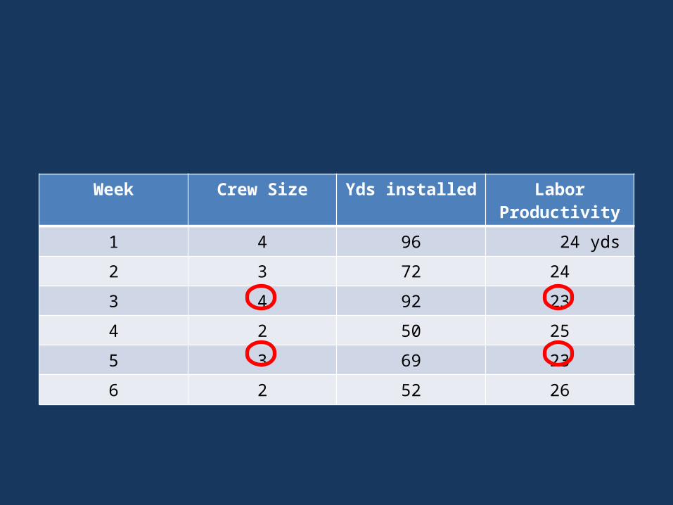
Week Crew Size Yds installed Labor Productivity

1 4 96 24 yds

2 3 72 24

3 4 92 23

4 2 50 25

5 3 69 23

6 2 52 26

Multifactor productivity• (Quantity of production)/

(multiple inputs, e.g., labor cost + materials costs + overhead)

• Problem 3, p 62

Week Output (in units) Workers Material (lbs)

1 30,000 6 450

2 33,600 7 470

3 32,200 7 460

4 35,400 8 480

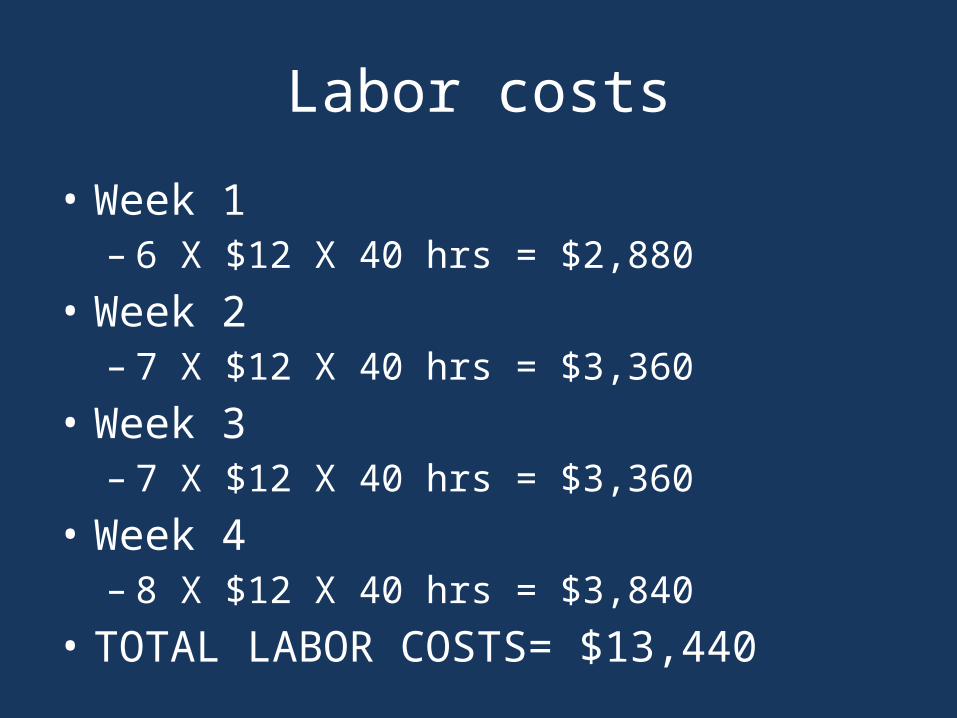
Labor costs

• Week 1– 6 X $12 X 40 hrs = $2,880

• Week 2– 7 X $12 X 40 hrs = $3,360

• Week 3– 7 X $12 X 40 hrs = $3,360

• Week 4– 8 X $12 X 40 hrs = $3,840

• TOTAL LABOR COSTS= $13,440

Overhead costs

• Week 1– 1.5 X $2,880 = $4,320

• Week 2– 1.5 X $3,360 = $5,040

• Week 3– 1.5 X $3,360 = $5,040

• Week 4– 1.5 X $3,840 = $5,760

• TOTAL OVERHEAD COSTS = $20,160

Material costs

• Week 1 – $6 X 450 = $2,700

• Week 2– $6 X 470 = $2,820

• Week 3– $6 X 460 = $2,760

• Week 4– $6 X 480 = $2,880

• TOTAL MATERIAL COSTS = $11,160

Week Output (in units)

Labor costs

Overhead costs

Material costs

Total costs

1 30,000

2 33,600

3 32,200

4 35,400

Week Output (in units)

Labor costs

Overhead costs

Material costs

Total costs

1 30,000 $2,880 $4,320 $2,700 $9,900

2 33,600 $3,360 $5,040 $2,820 $11,240

3 32,200 $3,360 $5,040 $2,760 $11,160

4 35,400 $3,840 $5,760 $2,880 $12,480

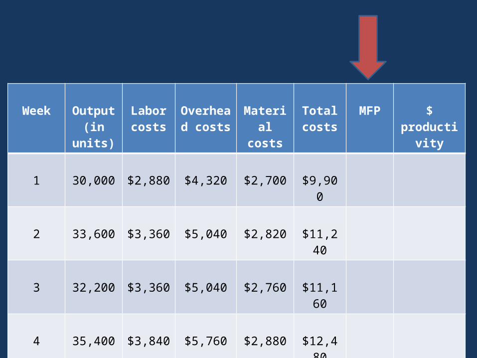
Week Output (in units)

Labor costs

Overhead costs

Material costs

Total costs

MFP $ productivity

1 30,000 $2,880 $4,320 $2,700 $9,900

2 33,600 $3,360 $5,040 $2,820 $11,240

3 32,200 $3,360 $5,040 $2,760 $11,160

4 35,400 $3,840 $5,760 $2,880 $12,480

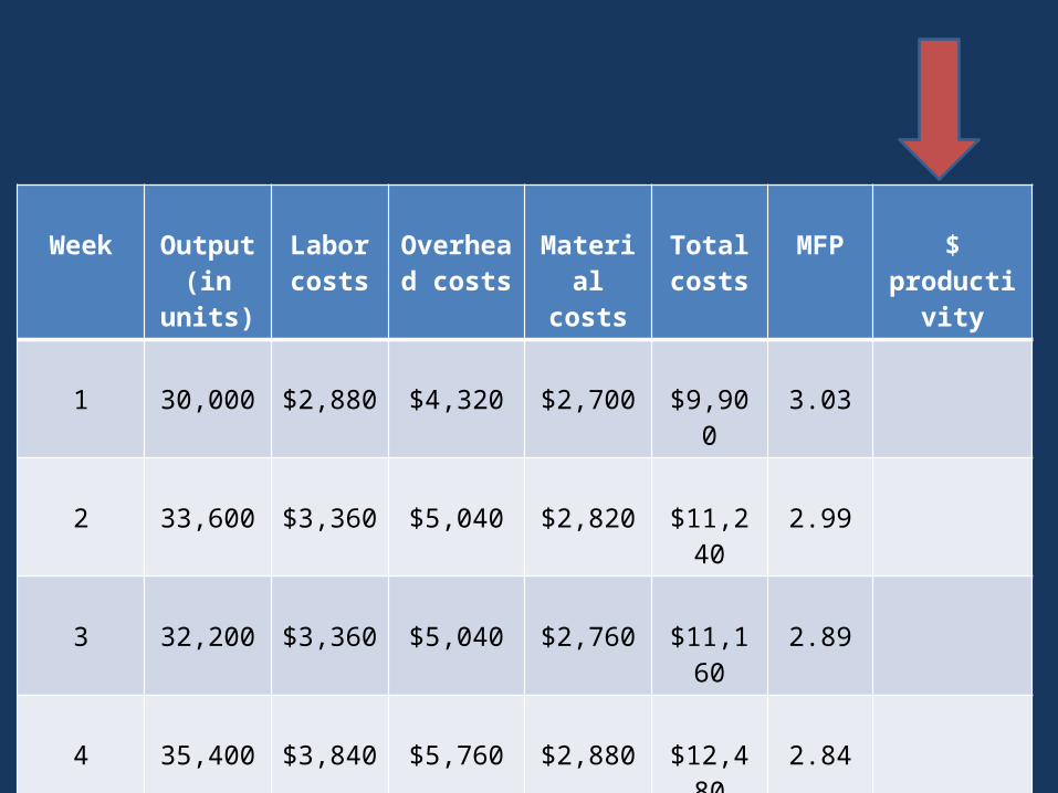
Week Output (in units)

Labor costs

Overhead costs

Material costs

Total costs

MFP $ productivity

1 30,000 $2,880 $4,320 $2,700 $9,900 3.03

2 33,600 $3,360 $5,040 $2,820 $11,240 2.99

3 32,200 $3,360 $5,040 $2,760 $11,160 2.89

4 35,400 $3,840 $5,760 $2,880 $12,480 2.84

Week Output (in units)

Labor costs

Overhead costs

Material costs

Total costs

MFP $ productivity

1 30,000 $2,880 $4,320 $2,700 $9,900 3.03 $424.20

2 33,600 $3,360 $5,040 $2,820 $11,240 2.99 $418.60

3 32,200 $3,360 $5,040 $2,760 $11,160 2.89 $404.60

4 35,400 $3,840 $5,760 $2,880 $12,480 2.84 $397.60

Productivity

• Rate of productivity growth (RPG)– ) ) x 100

RPG• Problem 6, p. 62• Current week – 160 units/40 hrs– Current productivity: 4 units/hr

• Previous week– 138 units/ 36 hrs– Previous productivity: 3.83 units/hr

• RGP– (4 units/hr – 3.83 units/hr) / 3.83 units/hr) = .044

– 4.4%

What is decision theory?

• Definition– Payoff table (certainty)– P. 159

POSSIBLE FUTURE DEMAND

Alternatives Low Moderate High

Small facility $10 $10 $10

Medium facility 7 12 12

Large facility (4) 2 16

What is decision theory?

• Basic concepts– Certainty vs uncertainty– Utility values• Ex: 1,000 units sold = utility of 1,000

– Or 50,000 (arbitrary decision)

– Expected utility• Probability X utility

Expected utility example

• Outcome 1: Utility = 100, probability = 75%• Outcome 2: Utility = -40, probability = 25%• Expected utility =

100 X .75 = 75 -40 X .25 = -10 75 + (-10) = 65

Decision making under uncertainty

• 4 possible decision criteria– Maximin• Best “worst” payoff

– Maximax• Best possible payoff

– Laplace• Equally lightly

– Minimax regret• Minimize “regret”

Decision making under uncertainty

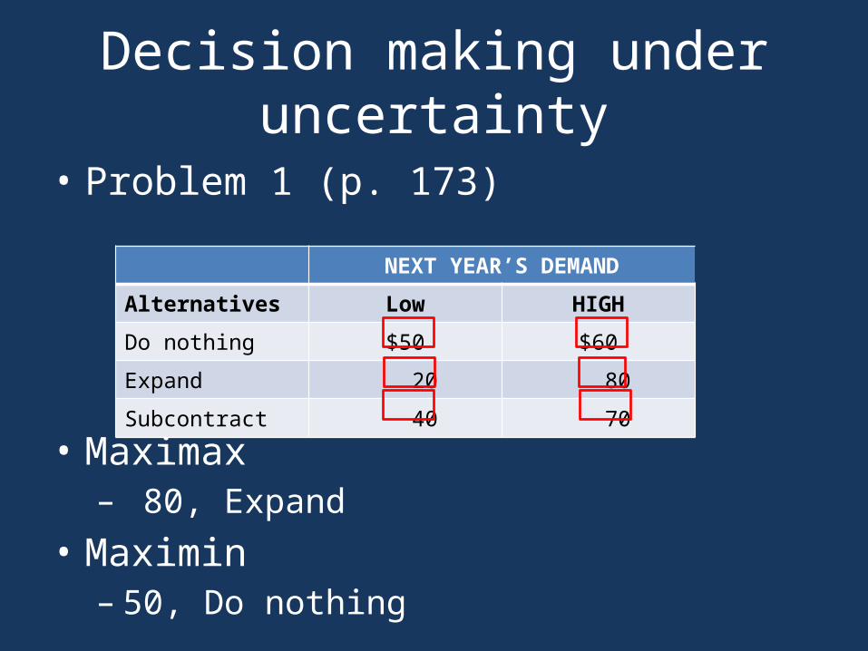
• Problem 1 (p. 173)

• Maximax – 80, Expand

• Maximin– 50, Do nothing

NEXT YEAR’S DEMAND

Alternatives Low HIGH

Do nothing $50 $60

Expand 20 80

Subcontract 40 70

Decision making under uncertainty

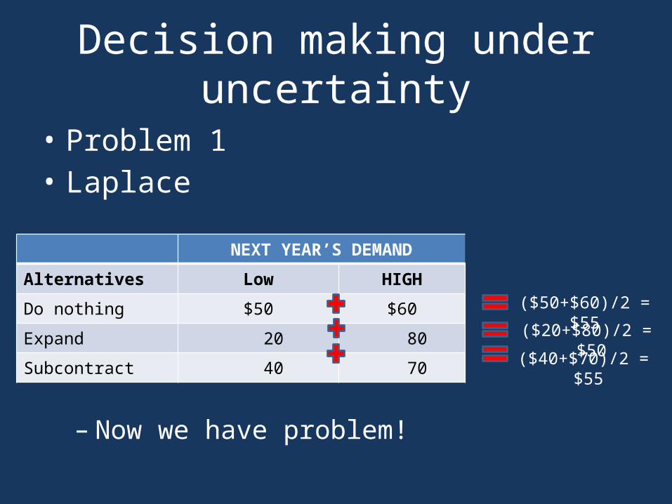
• Problem 1• Laplace

– Now we have problem!

NEXT YEAR’S DEMAND

Alternatives Low HIGH

Do nothing $50 $60

Expand 20 80

Subcontract 40 70($20+$80)/2 = $50

($50+$60)/2 = $55

($40+$70)/2 = $55

Decision making under uncertainty

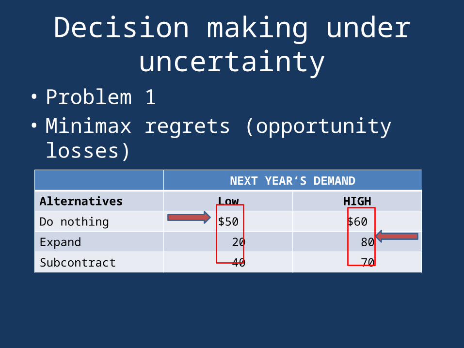
• Problem 1• Minimax regrets (opportunity losses)

NEXT YEAR’S DEMAND

Alternatives Low HIGH

Do nothing $50 $60

Expand 20 80

Subcontract 40 70

Decision making under uncertainty

• Problem 1• Minimax regrets

– subcontract

NEXT YEAR’S DEMAND

Alternatives Low HIGH WORST

Do nothing $50 - $50 = 0 $80 – 60 = 20 $20

Expand 50 – 20 = 30 80 – 80 = 0 30

Subcontract 50 – 40 = 10 80 – 70 = 10 10

Decision making under risk

• Problem 2(a)• EMV (expected profit)

• EMV(Do nothing): 50(.3) + 60(.7) = $57• EMV(Expand): 20(.3) + 80(.7) = $62• EMV(Subcontract): 40(.3) + 70(.7) = $61

NEXT YEAR’S DEMAND

Alternatives Low P(.30) HIGH P(.70)

Do nothing $50 $60

Expand 20 80

Subcontract 40 70

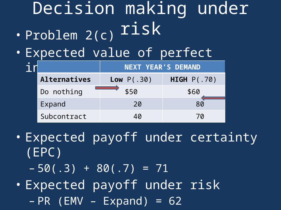
Decision making under risk• Problem 2(c)• Expected value of perfect information (EVPI)

• Expected payoff under certainty (EPC)– 50(.3) + 80(.7) = 71

• Expected payoff under risk – PR (EMV – Expand) = 62

• EVPI = 71 – 62 = 9

NEXT YEAR’S DEMANDAlternatives Low P(.30) HIGH P(.70)Do nothing $50 $60Expand 20 80Subcontract 40 70

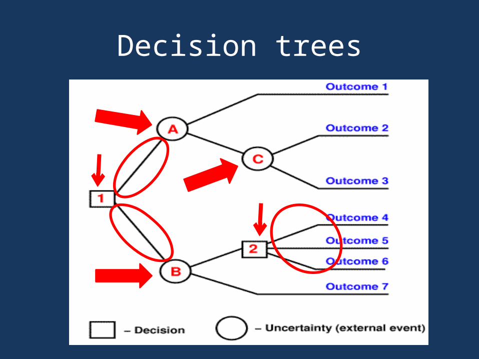
Decision trees

Decision trees

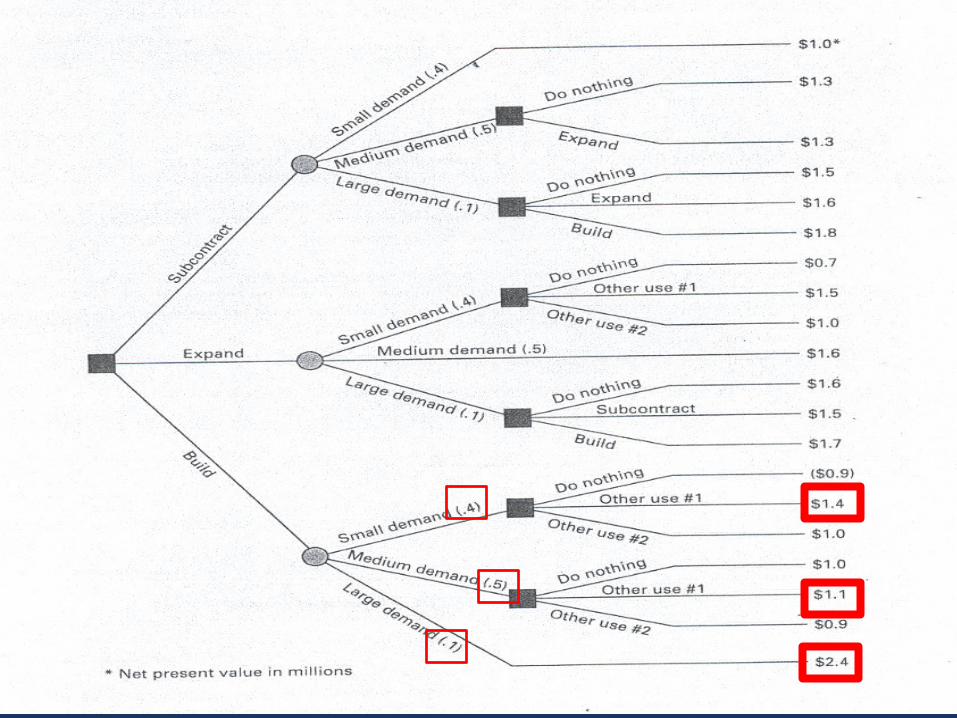
P5, p. 174

So what do we conclude?

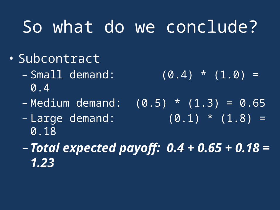
• Subcontract– Small demand: (0.4) * (1.0) = 0.4– Medium demand: (0.5) * (1.3) = 0.65– Large demand: (0.1) * (1.8) = 0.18–Total expected payoff: 0.4 + 0.65 + 0.18 = 1.23

So what do we conclude?

• Expand– Small demand: (0.4) * (1.5) = 0.6– Medium demand: (0.5) * (1.6) = 0.8– Large demand: (0.1) * (1.7) = 0.17–Total expected payoff: 0.6 + 0.8 + 0.17 = 1.57

So what do we conclude?

• Build– Small demand: (0.4) * (1.4) = 0.56– Medium demand: (0.5) * (1.1) = 0.55– Large demand: (0.1) * (2.4) = 0.24–Total expected payoff: 0.56 + 0.55 + 0.24 = 1.35

So what do we conclude?

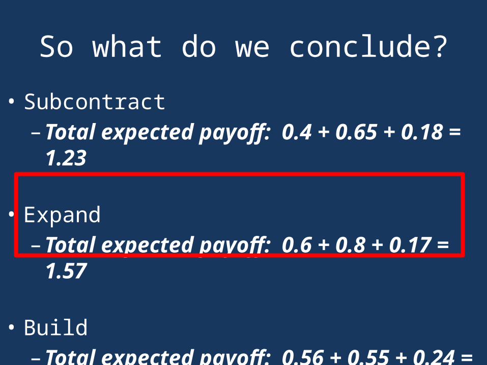
• Subcontract–Total expected payoff: 0.4 + 0.65 + 0.18 = 1.23

• Expand–Total expected payoff: 0.6 + 0.8 + 0.17 = 1.57

• Build–Total expected payoff: 0.56 + 0.55 + 0.24 = 1.35

Problem 12, p. 176

• Assume equal probabilities• Omit the leasing option

1

Build small

Build large

2

Lease

Expand

Demand low (.50)

Demand high (.50)

$700

$100

$500

$40

$2,000

Demand low (.50)

Demand high (.50)

Alternatives

• Maximin - best “worst”– Small: $500k– Large: $40K

• Maximax – best possible– Large: $2,000k

Lapace

• Small– .50($700) + .5($500) = $600

• Large– .50($40) + .50($2,000) = $1,020

1

Build small

Build large

2

Lease

Expand

Demand low (.50)

Demand high (.50)

$700

$100

$500

$40

$2,000

Demand low (.50)

Demand high (.50)

Minimax regretAlternatives Low High

Build Small $700 $500

Build Large $40 $2,000

Alternatives Low High

Build Small $700 - $700 = $0 $2,000 - $500 = $1,500

Build Large $700 - $40 = $660 $2,000 - $2,000 = $0