decision supporting of production planning and...

Proceedings of the TMCE 2008, April 21–25, 2008, Izmir, Turkey, Edited by I. Horváth and Z. Rusák Organizing Committee of TMCE 2008, ISBN ----

1

DECISION SUPPORTING OF PRODUCTION PLANNING AND CONTROL BY MEANS OF KEY PRODUCTION PERFORMANCE MEASURING INDICATORS

Tibor Tóth Department of Information Engineering

University of Miskolc [email protected]

Ferenc Erdélyi Gyula Kulcsár

Department of Information Engineering University of Miskolc

{erdelyi, kulcsar}@ait.iit.uni-miskolc.hu

ABSTRACT

In this paper we are dealing with one of the generic

issues in the area of production processes, namely

with the types of state characteristics supporting

decision making in production planning and control.

Flexible manufacturing has more and more

importance, which is able to adapt to the changing

requirements of demand and supply. In addition, the

demand for high-level readiness can be met only by

increasing quality and lower price. The PPC

modules of the present ERP systems are based upon

well-established mathematical models consisting of

production equations. Discussion of the production

equations demonstrated that in these models there

exist three performance indicator classes of great

importance. These are as follows: 1. Readiness for

delivery (Delivery capability) 2. Stock or WIP (work-

in-process) level 3. Utilization of resources. The

indicators depend on each other. Their

interdependencies are clearly demonstrated in

abstract systems – with one or multi machine – by the

so-called “production equations”. In the equations,

the production rates can be a parameter and play a

controlling role. A fundamental requirement of

manufacturing control policy is the stability of

production. In the case of stable production, we

deduce and proof a general relation among the

average of the performance indicators and the

average operation-rate parameter. For analyzing the

role of production performance indicators in the

decision making of different levels of production

planning and control a computer application has

been developed. Simulation experiments proved that

the key performance indicators of production

triangle give the best base of decision making on the

short and medium time horizons in productions

management. We would also like to present the main

findings of an industrial case study from our R&D

practice.

KEYWORDS

Manufacturing Systems; Production Planning and Control (PPC), Integration, Performance indicators.

1. INTRODUCTION

In the field of discrete manufacturing, it is observable that over efficient and profitable production, service level of customer’s requirements is becoming of greater and greater importance (Krajewski, J. and Ritzman, B., 1996). Agile manufacturing is a new term applied to manufacturers that have production processes being enable to respond quickly to customer needs and market changes. Agile manufacturers have to take it into consideration that high-level readiness for delivery that is reliable and accurate executing, carrying out or supplying customer orders are the most important part of enterprise performance measure. In manufacturing, there are two kinds of comprehensive management policy: make to order (MTO) and make to stock (MTS) (Buzacott, J. A. and Shanthikumar, J. G., 1993). Make to stock manufacturing is typically used in mass production, where the finished products are delivered from a warehouse when customer requests and purchases them. Mass production technology usually require automated part manufacturing and assembly lines, specialized workers, big lot sizes, automated quality checking, automated packing operations, and relatively high material inventory capacity. Agile manufacturers may use both policies for satisfying their accepted orders and utilizing their manufacturing resources. In the case of “customized mass production” paradigm (Scheer, A. W., 1994),

2 Tibor Tóth, Ferenc Erdélyi, Gyula Kulcsár

the firms plan their production partially for external direct orders arriving from logistic or shopping centres. However, to reach better delivery service they must make forecast for manufacturing to make safety stock and better utilization rate of bottleneck machines.

One of the Hungarian factories of a multinational firm carries out customized mass production. It is peculiar to this factory a large scale of product types, uncertainty of market demands, as well as rigorous conditions of the adaptation to the demands of customers (specification, packing, delivery dates). In the focus of production policy high level meeting the requirements of the customers is standing. Performance of production is measured by the quantity of products, stock level, keeping the deadlines according to the contracts, the number of setups and loading the labour capacities. It is also representative to production the variety of material demand, parallelism of machine capacities and dynamically controllable lot size. There is a continuous effort to improve production scheduling, therefore the application of dynamic production models come into prominence. The production models known from technical literature do not meet all these requirements to the expected extent.

We are taking part in an industrial development project (Real-time, Cooperative Enterprises, VITAL) that has been organized on three research and development fields. These are as follows:

1. Integrated production planning, resource

management and scheduling;

2. Handling of changes and disturbances at shop

floor execution level;

3. Cooperative supply chain and logistic networks.

The aim of the first cluster is to develop new extended manufacturing models and solving methods for optimal detailed scheduling application systems for a week, taking into consideration a lot of special conditions and constraints and goals (Kis, T., 2005).

The second cluster deals with handling of uncertainties at shop floor level with monitoring the state of the jobs and machines, taking actions as “behaviour based” control of the manufacturing systems and rescheduling the jobs for better performance measure.

The third cluster deals with the possibilities of developing a co-operative supply-chain, as well as

increasing the reliability of materials supply with vendor managed inventory control.

The project demonstrates well the efforts, which agile enterprises make in order to achieve their strategic goals in the fields of planning and control for production systems and processes. These tasks, in the majority of cases, can only be solved by means of a new approach, new models, and new applications of information engineering and technology. The second, third, and fourth sections of this paper introduce strategic aspects of decision support for production planning and control using the concept of “production triangle” as a main tool for performance measurement. The next sections will present our model for a production system and its long-time performance analysis. These will be followed by a detailed discussion of the production triangle equation for the cases of one and more than one machine. Our research assumes a stable flow shop type system with known production intensity data. The next sections show how this performance measuring method supports the production planning by handling the uncertainties and disturbances at shop floor execution level. We also present a new software application for solving the performance measuring, scheduling and rescheduling tasks.

2. DECISION SUPPORTING OF PRODUCTION PLANNING AND CONTROL

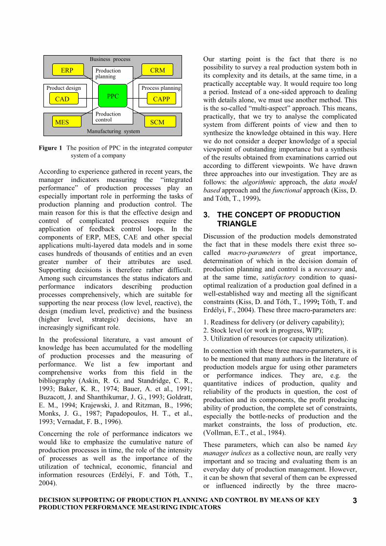
The introduction of computer application systems is an everyday task today, for the small- and medium-sized companies as well. Effective technical and management decisions, however, require well-adjusted computer models and a suitable database. All this, in turn, require further fine-tuning and improvement of the modelling of production processes. Production design is the most complex of the three technical planning processes (product, technology and production planning) and it is the most difficult to model it. It presupposes the detailed and exact plans of the products (and/or services) in demand by the buyer (by the market) as well as the exact knowledge of the supplier and acquisition processes necessary for the production of these. Besides, production planning – through a common model – is closely related to business decisions and production control (Figure 1.).

DECISION SUPPORTING OF PRODUCTION PLANNING AND CONTROL BY MEANS OF KEY

PRODUCTION PERFORMANCE MEASURING INDICATORS 3

ERP

Business process

Product design

Manufacturing system

MES

CAD

Process planning

CAPP

Productionplanning

Productioncontrol

PPC

CRM

SCM

Figure 1 The position of PPC in the integrated computer system of a company

According to experience gathered in recent years, the manager indicators measuring the “integrated performance” of production processes play an especially important role in performing the tasks of production planning and production control. The main reason for this is that the effective design and control of complicated processes require the application of feedback control loops. In the components of ERP, MES, CAE and other special applications multi-layered data models and in some cases hundreds of thousands of entities and an even greater number of their attributes are used. Supporting decisions is therefore rather difficult. Among such circumstances the status indicators and performance indicators describing production processes comprehensively, which are suitable for supporting the near process (low level, reactive), the design (medium level, predictive) and the business (higher level, strategic) decisions, have an increasingly significant role.

In the professional literature, a vast amount of knowledge has been accumulated for the modelling of production processes and the measuring of performance. We list a few important and comprehensive works from this field in the bibliography (Askin, R. G. and Standridge, C. R., 1993; Baker, K. R., 1974; Bauer, A. et al., 1991; Buzacott, J. and Shanthikumar, J. G., 1993; Goldratt, E. M., 1994; Krajewski, J. and Ritzman, B., 1996; Monks, J. G., 1987; Papadopoulos, H. T., et al., 1993; Vernadat, F. B., 1996).

Concerning the role of performance indicators we would like to emphasize the cumulative nature of production processes in time, the role of the intensity of processes as well as the importance of the utilization of technical, economic, financial and information resources (Erdélyi, F. and Tóth, T., 2004).

Our starting point is the fact that there is no possibility to survey a real production system both in its complexity and its details, at the same time, in a practically acceptable way. It would require too long a period. Instead of a one-sided approach to dealing with details alone, we must use another method. This is the so-called “multi-aspect” approach. This means, practically, that we try to analyse the complicated system from different points of view and then to synthesize the knowledge obtained in this way. Here we do not consider a deeper knowledge of a special viewpoint of outstanding importance but a synthesis of the results obtained from examinations carried out according to different viewpoints. We have drawn three approaches into our investigation. They are as follows: the algorithmic approach, the data model based approach and the functional approach (Kiss, D. and Tóth, T., 1999).

3. THE CONCEPT OF PRODUCTION TRIANGLE

Discussion of the production models demonstrated the fact that in these models there exist three so-called macro-parameters of great importance, determination of which in the decision domain of production planning and control is a necessary and, at the same time, satisfactory condition to quasi-optimal realization of a production goal defined in a well-established way and meeting all the significant constraints (Kiss, D. and Tóth, T., 1999; Tóth, T. and Erdélyi, F., 2004). These three macro-parameters are:

1. Readiness for delivery (or delivery capability); 2. Stock level (or work in progress, WIP); 3. Utilization of resources (or capacity utilization).

In connection with these three macro-parameters, it is to be mentioned that many authors in the literature of production models argue for using other parameters or performance indices. They are, e.g. the quantitative indices of production, quality and reliability of the products in question, the cost of production and its components, the profit producing ability of production, the complete set of constraints, especially the bottle-necks of production and the market constraints, the loss of production, etc. (Vollman, E.T., et al., 1984).

These parameters, which can also be named key manager indices as a collective noun, are really very important and so tracing and evaluating them is an everyday duty of production management. However, it can be shown that several of them can be expressed or influenced indirectly by the three macro-


parameters while the others are strictly influenced by economic and selling decisions, and therefore influence the model of production process in an indirect way only.

Taking into consideration the profit producing requirements of market economy, production planning tasks have to be solved such a way that the following requirements should be met:

(1) The readiness for delivery should be acceptable to the customer in every case (in general, to ensure as short a term of delivery as possible);

(2) The stock level should as low as possible (this is valid for all the raw materials, semi-finished products, finished products/articles, spare parts etc.);

(3) The capacity utilization of production equipment and other homogeneous workplaces should be between the required limits prescribed by the enterprise management.

Adapting this task to the environment and surroundings of a given enterprise, we usually get a large-size quasi-optimization problem. Having modelled the task from a mathematical point of view it can be recognized that readiness for delivery, stock level and capacity utilization are functions of the so-called “dependent orders”, i.e. of the manufacturing orders and purchasing orders.

The basic task of the PPC system is to determine manufacturing and purchasing orders taking into consideration the constraints of the current production environment in such a way that the given industrial enterprise (part manufacturing and assembly) should operate near to the “optimal working point” from the aspects of readiness for delivery, stock level and capacity utilization. This is made perceptible, though in a very simplified manner, in Figure 2.

MACHINES

INPUT STORAGE

DEMANDS

OUTPUT STORAGE

time

OPERATIONSORDERS

THROUGHPUT

WORKPLACE

RAW MATERIAL FINISHED PRODUCTS

UTILIZATION PRODUCTIONTRIANGLEWORK IN

SATISFYING OF

time timeFLOW OR THROUGHPUTPROCESSTIME

J1

J2

J3

M

M

NGantt chart Gantt chart

T(O)

N(O) U(O)

O

U(O)

T1

2T

3T

1

2

3

M

M

1

2

3

PRODUCTION CONTROL

INTERNAL

ORDERSEXTERNAL

PRODUCTION

PLANNING AND

SCHEDULING

Figure 2 “Production Triangle” model

The production process can also be modelled in a mathematical way with the partial models of the three macro-parameters in a close interrelationship with one another. These macro-parameters are as follows:

• Readiness for delivery, according to definition, is the reciprocal value of the time that passes from the acceptance of a given external order to the due date fixed in the delivery contract. It is usual to name this parameter the “time window” of production planning. Of course, this length of time can only be determined in an approximate way when entering into a contract, starting from the due date of delivery and the prospective value of the lead-time. (The unit of measurement is usually 1/day).

• Stock level (or inventory level), as a collective noun, means the quantity/amount of manufacturing lots/runs, i.e. all the products, assembly units, parts, raw materials and other necessary auxiliaries in the store rooms, as well as in the manufacturing and assembly workplaces, at a given point of time. The higher the stock level the greater the working capital demands of stock. Stock level is in close relationship with the amount of works in progress (WIP).

• Capacity utilization means the percentile engagement/loading of operation-time capacity of the manufacturing places in a given time period, including all the workshops, working groups, workplaces and vehicles, which form an independent



unit from the point of view of scheduling. Because capacities are always limited, the constraints related to them are indispensable.

The macro-parameters of production, as can be understood, are partially dependent on how and to what extent the external order book changes. In addition, they are partially dependent on the method for production planning and controlling how and in what way the internal orders are scheduled, taking into consideration all the essential constraints of production, both in time and in capacity, as well as factors related to the specific technological processes employed.

It is obvious that all the mathematical models and algorithms used in PPC are necessarily of approximate character. The generic task of production planning and control is an approximate optimization of the production process, in which (1) the variable of optimization is the changing set of the internal orders released (be careful: this set is changing not only in its amount but in time as well), i.e. production schedule, and (2) the objective function of optimization is a complicated function of the three macro-parameters previously defined.

By means of this approach, we would like to answer the question of what kind of algorithmic relationships can be defined in the field of production planning and control. To achieve this objective we examine the so-called production ability of a given enterprise suitable to meet the requirements of production and try to formulate relationships related to it. By way of illustration, the symbolic description of PPC problem can be the following:

Let us introduce the symbol ( )tO for notation of the

set of internal orders at a point of time optional but fixed after selection. Every order is a data set belonging to a decision event, which includes the identifier of the ordered item, the ordered quantity and the data of the time window allowed for the performance of order. Let us denote the macro-parameters of production dependent on the set of internal orders as follows:

( )( )tON – the set of WIP level parameters,

( )( )tOU – the set of machine utilization parameters,

( )( )tOT – the set of readiness for delivery

parameters.

It is obvious that any macro-parameter as a component of the objective function to be synthesized in some kind of way cannot be expressed

by means of mathematical operations carried out on the set of internal orders. Similarly, it is impossible to determine a set of internal orders starting from the required value of the objective function, which belongs to an optimum level of meeting of all the constraints. Because of interconnections of the macro-parameters that are the independent variables of the objective function, we can state that if any macro-parameter would get priority in distribution of the internal orders this fact could influence the other two in a disadvantageous way. Hence, there is a need for defining a production policy that determines the weights of the macro-parameters of production within the complex production goal. Pareto optimization would also be possible in principle (Ehrgott, M., 2000). A new, advantageous approach suitable for solving multi-objective production scheduling problems was proposed by Kulcsár, et al. (2007).

The PPC problem can be symbolized in the following manner: it is to be determined the set of internal orders ( )stO0 related to the point of time st , for

which ( )( ) optimumtO s →Φ 0 , and, at the same time, the

values of the components ( )

( )( )( )( )

s

s

s

tOT

tOU

tON

0

0

0 )(

meet all the prescribed constraints.

As can be seen, solving the optimization task is strongly model-dependent and, in addition to the selection of an objective function, it depends on the feasibility of meeting the constraints as well. The model conduces to NP-hard discrete or mixed integer mathematical programming problems for which, in the overwhelming majority of cases, a solution cannot be guaranteed even using very fast processors. In general, solving the problem is possible only when we give equations, inequalities and other relationships for the elements of sets of the macro-parameters of production by means of which the production conditions can be asserted step-by-step.

The algorithmic approach defines interconnections of the main characteristics of the production triangle in the form of so-called “production equations”. They are (listed only): (1) stock equations; (2) component-demand equations; (3) capacity-demand equations; (4) equations regarding the throughput-time of manufacturing; (5) due-date equations.


To determine the set of internal orders ( )tO it is

necessary to invert the system of production equations. From the mathematical model, it has appeared that inverting can only be executed for simple tasks of small size because of the great number of variables and non-linearity of the relationships, as well as the complexity of the set of constraints to be taken into consideration. In spite of this fact, the model is still of great importance because it allows the creation of a control loop, where the quasi-optimum solution can be approximated by using heuristics, simulation method, iterative searching and feedback. Evaluation and fine-tuning of the system requires interactive human intervention in general, and here heuristics or a suitable procedure based on some kind of method of Operations Research is needed.

4. PERFORMANCE MANAGEMENT

The performance indices of manufacturing system models can be classified into six basic groups. They are as follows: 1. Stock (or WIP) level. 2. Capacity utilization. 3. Delivery capability. 4. Throughput volume. 5. Finished product quality. 6. Production cost or profit. The first three indexes compose the “production triangle”.

The indices are dependent on each other. Their interdependencies are clearly demonstrated even in a “one-machine based” abstract system by the so-called “production equations” firstly founded by Little and analysed in details in the work of Buzacott, J.A., and Shanthikumar,J.G. (1993). In the aggregate production planning the rate (or rate profile) of the high-level production activities constitutes the basis of project-like production scheduling. At shop floor level, three rates are the input information basis of scheduling, namely: 1. the arrival rate of the internal orders (works). 2. The demand rate given for the works. This is the quotient of the time load depending on the lot size, and the duration of deadline window. 3. The production rate that is the inverse of throughput time. At the level of the workplaces the rate is a parameter of technology process planning that can be optimized on the basis of different objective functions, taking the prevailing constraints into consideration. The planned rate, in the case of machining, influences not only the quality of product but the operation time and the tool consumption as well. The rate of a bottleneck, especially in case of multi-operation production routing, influences the characteristics of the

realizable schedules largely. The long-term goal of production is the maximum of profit. However, this goal can only be achieved by a series of production goals realizable in shorter periods. These short-term goals are connected with the output characteristics of production. These performance indices are also named “natural” indices and recently “logistic performance” indices have been suggested. The up-to-date Manufacturing Execution Systems (MES), by means of production monitoring data acquisition, observe forming the performance indices of Production Triangle through the comparison of planned and realized values. Hence, the indices have an important role not only in the optimization tasks of proactive production planning period but they play the role of the error signals of reactive production control in the phase of execution. Therefore, it is very important for production planners and dispatchers to know capabilities and limits of their factory and workshop unambiguously and to recognize the sources of those conflicts, which appear in the course of measuring the performance of production.

5. MODEL FOR PRODUCTION PLANNING AND CONTROL

In the formal basic model we know the set of machines (resources): { }jmM = , mj ,...,1= ,

+∈Zm ; the set of inside orders and jobs: { }iJJ = ,

ni ,...,1= , +∈Zn , every job consists of operations

joined in a line: { }jioO ,= , and every operation

requires ji ,τ time, Rji ∈,τ . The objective function,

measuring make to stock, is mostly “makespan”:

min);min()max( →−= fTTf AiCi , where CiT is

the time when job i is finished and AiT is the time

when job i arrives (is released). In the case of manufacturing to stock, the objective function actually means minimizing the total time of delay:

min),,0max(1

→−=∑=

fTTfn

i

DiCi , where DiT is

the deadline of job i. Let us assume that the production rate of the operations jiq , is constant:

ji

jiq,

,

1

τ= [piece/min]. (1)

In modern flexible mass production, the so-called “Flow shop” models have a special role. The



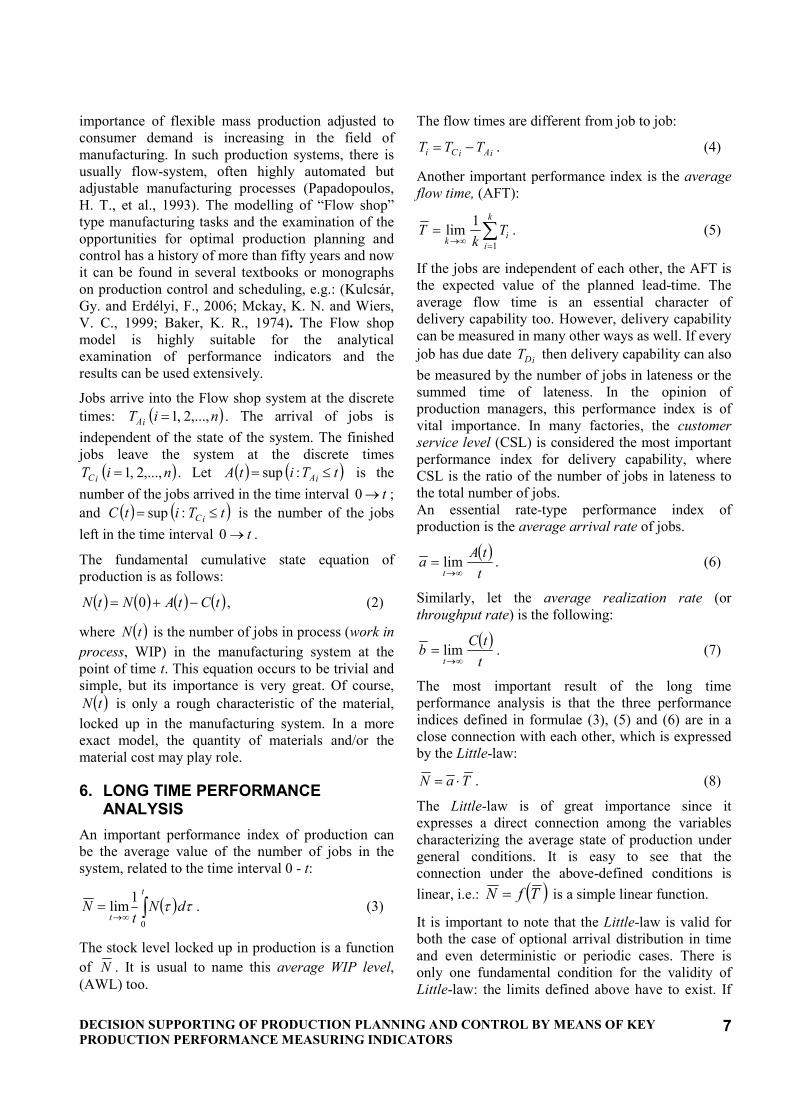
importance of flexible mass production adjusted to consumer demand is increasing in the field of manufacturing. In such production systems, there is usually flow-system, often highly automated but adjustable manufacturing processes (Papadopoulos, H. T., et al., 1993). The modelling of “Flow shop” type manufacturing tasks and the examination of the opportunities for optimal production planning and control has a history of more than fifty years and now it can be found in several textbooks or monographs on production control and scheduling, e.g.: (Kulcsár, Gy. and Erdélyi, F., 2006; Mckay, K. N. and Wiers, V. C., 1999; Baker, K. R., 1974). The Flow shop model is highly suitable for the analytical examination of performance indicators and the results can be used extensively.

Jobs arrive into the Flow shop system at the discrete times: ( )niT

iA,...,2,1= . The arrival of jobs is

independent of the state of the system. The finished jobs leave the system at the discrete times

( )niTiC

,...,2,1= . Let ( ) ( )tTitAiA≤= :sup is the

number of the jobs arrived in the time interval t→0 ; and ( ) ( )tTitC

iC≤= :sup is the number of the jobs

left in the time interval t→0 .

The fundamental cumulative state equation of production is as follows:

( ) ( ) ( ) ( )tCtANtN −+= 0 , (2)

where ( )tN is the number of jobs in process (work in

process, WIP) in the manufacturing system at the point of time t. This equation occurs to be trivial and simple, but its importance is very great. Of course, ( )tN is only a rough characteristic of the material,

locked up in the manufacturing system. In a more exact model, the quantity of materials and/or the material cost may play role.

6. LONG TIME PERFORMANCE ANALYSIS

An important performance index of production can be the average value of the number of jobs in the system, related to the time interval 0 - t:

( ) ττ dNt

Nt

t∫∞→

=0

1lim . (3)

The stock level locked up in production is a function

of N . It is usual to name this average WIP level, (AWL) too.

The flow times are different from job to job:

iAiCi TTT −= . (4)

Another important performance index is the average flow time, (AFT):

∑=∞→

=k

i

ik

Tk

T1

1lim . (5)

If the jobs are independent of each other, the AFT is the expected value of the planned lead-time. The average flow time is an essential character of delivery capability too. However, delivery capability can be measured in many other ways as well. If every job has due date

iDT then delivery capability can also

be measured by the number of jobs in lateness or the summed time of lateness. In the opinion of production managers, this performance index is of vital importance. In many factories, the customer service level (CSL) is considered the most important performance index for delivery capability, where CSL is the ratio of the number of jobs in lateness to the total number of jobs. An essential rate-type performance index of production is the average arrival rate of jobs.

( )t

tAa

t ∞→= lim . (6)

Similarly, let the average realization rate (or throughput rate) is the following:

( )t

tCb

t ∞→= lim . (7)

The most important result of the long time performance analysis is that the three performance indices defined in formulae (3), (5) and (6) are in a close connection with each other, which is expressed by the Little-law:

TaN ⋅= . (8)

The Little-law is of great importance since it expresses a direct connection among the variables characterizing the average state of production under general conditions. It is easy to see that the connection under the above-defined conditions is

linear, i.e.: ( )TfN = is a simple linear function.

It is important to note that the Little-law is valid for both the case of optional arrival distribution in time and even deterministic or periodic cases. There is only one fundamental condition for the validity of Little-law: the limits defined above have to exist. If


the arrival process is a Markov-process in time, the conditions are valid. Of course, the law says nothing about the fluctuation of stock level and lead times.

7. THE STABILITY OF PRODUCTION

A fundamental requirement of manufacturing control policy is the stability of production. Production is stable if the number of jobs in the system remains finite for an optional long time. In this case, the buffer dimensions can be realized and the orders, sooner or later, by chance in lateness, will be performed with absolute certainty.

( ) *lim NNt

tN

t≤=

→∞ (9)

where *N is a finite constant.

For stable production there is an equilibrium between the average arrival rate of jobs and the through put rate of finished jobs, i.e.,

ba = . (10)

This condition can be performed if and only if the average value of operation times of the technology operations to be realized satisfies a special constraint.

qa ≤ , (11)

where q is the average operation rate:

τ/q 1= (12)

∑=

=n

i

in 1

*1ττ , where ∑

=

=m

j

ijim 1

* 1ττ .

Inequality (11) expresses the trivial, but fundamental assumption that the content of the intermediate buffers between machines (workplaces) can not remain finite if the jobs arrive with a rate greater than the production rate of workplaces (job-processing rate).

The third important performance index is then the average utilization of resources of the workplace. This index denoted by u is the quotient of the time spent in work and the total time available.

It is provable (e.g. see: Kulcsár, Gy. and Erdélyi, F., 2006) that for the machine j:

( )

j

tA

i

jit

jq

a

tu == ∑

=∞→

1

1lim τ . (13)

It is obvious that utilization cannot be greater than 100 % and in case of stable production, the following condition is valid:

1/ ≤jqa .,...,1 mj = (14)

Inequality (14) means, that every resources can be loaded to their capacity limits only. This is the base of capacity constraints in any manufacturing optimal scheduling task.

8. THE “PRODUCTION TRIANGLE” EQUATION FOR ONE MACHINE CASE

If relationship (14) is performed, i.e., production is stable, we have:

qua ⋅= . (15)

Using the Little-law, it can be written:

TuqN ⋅⋅= . (16)

We call relationship (16) “production triangle” equation. It expresses that in the case of the operation rates given in the technology process plans, as well as the lot sizes and due dates given in the orders the three performance indices of production triangle can not be improved independently of each other.

J

J

1

n

u

N

TINPUT BUFFER

M1

OUTPUT BUFFER

J i

O

O

O

O1

n

time

J

J

J

J

1

2

i

n

Gantt chart

2

i

ts= max T

Ci

Figure 3 One machine production system If, for example, the jobs have rigorous deadlines and the condition

iDiCTT ≤ must be performed for every

i then machine utilization and stock level cannot be improved at the same time.

Similarly, if we want to keep machine utilization at high level then stock level and flow time cannot be decreased at the same time (Kiss, D. and Tóth, T., 1999; Kulcsár, Gy. and Erdélyi, F. 2006).

According to our theoretical and simulation experience, the curves represented by the production



characteristics TuqN ⋅⋅= , ( )Nfu = and

( )NfT = will remain valid for multi-machine flow

shop systems too.

9. ORDERING-ARRIVAL IN GROUPS AND PREDICTIVE SCHEDULING FOR ONE MACHINE

Ordering-arrival in groups and predictive model-based scheduling are quite frequent in industrial practice. Jobs arrive in groups, at the same time, at t=0. They are scheduled by optimizing the scheduling plan. The objective function can be e.g. the average through put time or the minimization of the number of jobs in process on average. If every job has a deadline, we can make a schedule for the minimal late jobs or some function of the differences from the deadline.

In the case of one machine, makespan

)min()max( AiCims TTt −= =∑=

n

i

ci

1

τ , (17)

does not depend on the scheduling. The average job number in the system is an average based on time, which can be calculated with the help of the “load” function.

)(1)(1)( CiAii TtTttN −−−= and ∫=

=mst

t

ii TdttN0

)( .

Using the above:

∫→=

t

ttdN

tN

ms0

)(1

lim ττ ∫ ∑= =

=mst

t

n

i

i

ms

dNt

0 1

)(1

ττ .

Exchanging the addition and the integration:

ms

n

i

i

t

T

N∑== 1 . (18)

The utilization of machines is now, of course, u =1 (100%) since on the 0→tms horizon there is no waiting time for the machines.

11 ===∑=

ms

M

ms

n

i

i

ttu

ττ

. (19)

The average production intensity:

∑=

==n

i

iM

M

n

nq

1

/

1

ττ. (20)

The average through put time is a set average:

n

T

T

n

i

i

i

∑== 1 , (21)

where n is the number of jobs launched in groups. Using the above:

ms

n

i

i

n

i

i

iM

ms

n

i

i

t

nTuq

t

T

N∑

∑

∑=

=

= =⋅⋅== 1

1

1 .

τ

τn

Tn

i

i∑=1. N

t

T

ms

n

i

i

==∑=1 .

The production triangle relationship therefore does exist.

It can be proved – although we will not go into details here and now – that the relationship exists in the case of parallel machine capacities and production interrupted through periods of waiting as well.

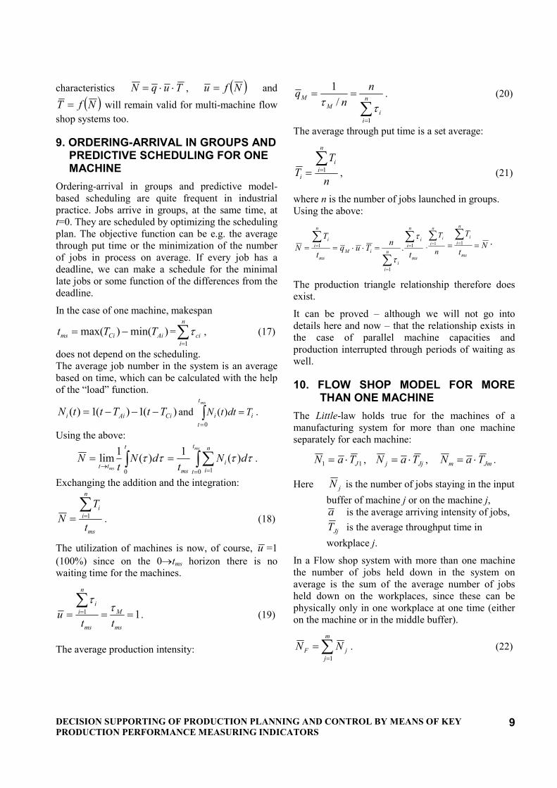
10. FLOW SHOP MODEL FOR MORE THAN ONE MACHINE

The Little-law holds true for the machines of a manufacturing system for more than one machine separately for each machine:

11 JTaN ⋅= , Jjj TaN ⋅= , Jmm TaN ⋅= .

Here jN is the number of jobs staying in the input

buffer of machine j or on the machine j, a is the average arriving intensity of jobs,

JjT is the average throughput time in

workplace j.

In a Flow shop system with more than one machine the number of jobs held down in the system on average is the sum of the average number of jobs held down on the workplaces, since these can be physically only in one workplace at one time (either on the machine or in the middle buffer).

∑=

=m

j

jF NN1

. (22)


10

INPUT BUFFER

... ...

OUTPUT BUFFER

M1 M

jM

m

Gantt chart

M1

Mj

Mm

TJ1

Gantt chart

J1

Jn

iJ

ts= max TCi

J1

Jn

iJ

T

u

N

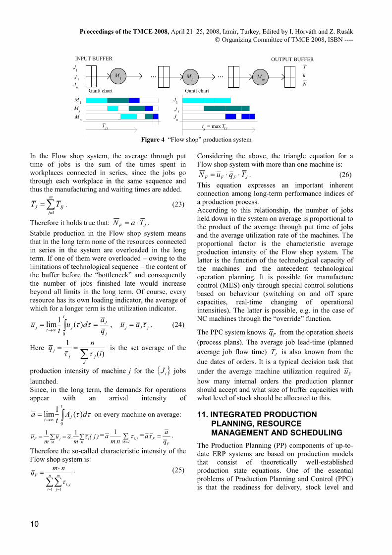
Figure 4 “Flow shop” production system

In the Flow shop system, the average through put time of jobs is the sum of the times spent in workplaces connected in series, since the jobs go through each workplace in the same sequence and thus the manufacturing and waiting times are added.

∑=

=m

j

JjJ TT1

. (23)

Therefore it holds true that: JF TaN ⋅= .

Stabile production in the Flow shop system means that in the long term none of the resources connected in series in the system are overloaded in the long term. If one of them were overloaded – owing to the limitations of technological sequence – the content of the buffer before the “bottleneck” and consequently the number of jobs finished late would increase beyond all limits in the long term. Of course, every resource has its own loading indicator, the average of which for a longer term is the utilization indicator.

∫ ==∞→

t

j

Jj

tj

q

adu

tu

0

)(1

lim ττ , jJj au τ= . (24)

Here ∑

==

J

jj

ji

nq

)(

1

ττ is the set average of the

production intensity of machine j for the { }iJ jobs

launched. Since, in the long term, the demands for operations appear with an arrival intensity of

∫→∞=

t

Jt

dAt

a0

)(1

lim ττ on every machine on average:

)j(m.au

mu

Mi

MjF ∑∑ == τ

11 = ∑×JM

j,in.m

a τ1 =

F

Fq

aa =τ .

Therefore the so-called characteristic intensity of the Flow shop system is:

∑∑= =

⋅=

n

i

m

j

ji

F

nmq

1 1,τ

. (25)

Considering the above, the triangle equation for a Flow shop system with more than one machine is:

JFFF TquN ⋅⋅= . (26)

This equation expresses an important inherent connection among long-term performance indices of a production process. According to this relationship, the number of jobs held down in the system on average is proportional to the product of the average through put time of jobs and the average utilization rate of the machines. The proportional factor is the characteristic average production intensity of the Flow shop system. The latter is the function of the technological capacity of the machines and the antecedent technological operation planning. It is possible for manufacture control (MES) only through special control solutions based on behaviour (switching on and off spare capacities, real-time changing of operational intensities). The latter is possible, e.g. in the case of NC machines through the “override” function.

The PPC system knows Fq from the operation sheets

(process plans). The average job lead-time (planned

average job flow time) JT is also known from the

due dates of orders. It is a typical decision task that

under the average machine utilization required Fu

how many internal orders the production planner should accept and what size of buffer capacities with what level of stock should be allocated to this.

11. INTEGRATED PRODUCTION PLANNING, RESOURCE MANAGEMENT AND SCHEDULING

The Production Planning (PP) components of up-to-date ERP systems are based on production models that consist of theoretically well-established production state equations. One of the essential problems of Production Planning and Control (PPC) is that the readiness for delivery, stock level and



utilization of production resources are such complex state variables (macro-parameters) that they cannot be managed independently of each other, while disturbances and uncertainties can occur in production processes. It is easy to see that unexpected events cannot be anticipated before executing the processes. Therefore realizable PPC systems are of hierarchical structure, in which there are a lot of constrains and multi objectives to be reached and long, medium and short term production planning has to be combined with real time production control (Vollman, E.T. et al., 1984; Monks, J. G., 1987; Kiss, D. and Tóth, T., 1999). It is to be recognized the fact that the objectives defined at a higher level of hierarchy are transformed to the lower levels in form of constraints.

To solve a multi-objective scheduling problem, it is necessary to answer an important question: What does it mean: “good” schedule? It is not easy to specify the answer in mathematical form because of in real-life situations there are many objectives (based on delivery capability, machine utilization rate, and stock level) and they are usually conflicting. The actual importance of objectives can vary frequently in time. Two authors of the present three suggest a typical appearance of the problem in customized mass production (Kulcsár, Gy. et al., 2005).

It comes into view that lots of flexible flow shop model exist in the literature, but they do not consider all the requirements of customized mass production (Nyhuis, P. et al., 2005; Sbalzarini, I. F., et al., 2000; Baykasoğlu, A., et al., 2002; Geiger, M. J., 2006; Loukil, T. et al., 2005). The conventional flow shop model has to be extended to a new model that supports execution steps, alternative technological routes, and unrelated parallel machines with different capabilities. Sequence dependent setup times, special job characteristics and different objective functions are also considered at the same time. For the scheduling task, a new approach is developed to solve multi-objective production scheduling and rescheduling problems. Furthermore the relationship between production goals and heuristic solving methods in an extended flexible flow shop environments is also investigated (Kulcsár, Gy. and Erdélyi, F., 2006). We define production goal by specifying objective functions and apply special production constraints for the extended flow shop scheduling model. The proposed method focuses on creating near-optimal feasible schedule considering multiple objectives and it is based on the well-known

taboo search meta-heuristics. Moreover, we use an advanced structure of taboo-list with new relational and neighbourhood operators and redefine the multi-objective aim for rescheduling tasks. The extended flexible flow shop scheduling problem (EFFS) is difficult to solve because of its combinatorial nature. The model inherits the difficulties of the classical flow shop (FS) and the flexible flow shop (FFS) models. Additionally, numerous strange features appear because of special extensions. The scheduling task consists of batching, assigning, sequencing and timing parts. We developed a new integrated approach to solve all the sub-problems as a whole without decompositions. In our approach, all the issues are answered simultaneously.

12. HANDLING OF CHANGES AND DISTURBANCES ON SHOP FLOOR EXECUTION LEVEL

A mass manufacturer faces three main sources of uncertainty: market, manufacturing process and supply chain uncertainty. In conventional production management, these problems are addressed by hierarchical control, reserved capacity and safety buffers. The main disadvantage of these approaches is that they fail to consider the level of uncertainness of the current market environment and the significance of feedback from the manufacturing process level. In the long run, these approaches weaken the competitiveness and profitableness of the manufacturer. In the course of planning and scheduling of customized mass production, three important uncertainties must be taken into account. They are as follows: 1. Uncertainty of market orders, both in quantity

and urgency; 2. Uncertainty of materials supply because of the

risk of services of the suppliers; 3. Uncertainty of production lines and, from time to

time, uncertainty of the available skilled labour.

To make a competent decision in manufacturing systems two matters have to be considered: the actual status of manufacturing resources and of material flow. Any decisions that are made without this criterion will lead to an error-prone behaviour. Moreover, invariability of such status information among the decision makers has to be guaranteed in order to achieve collaborative actions to resolve problems. In case all participants of a decision making system comprehend situations invariably and each participant possesses a well defined scope of


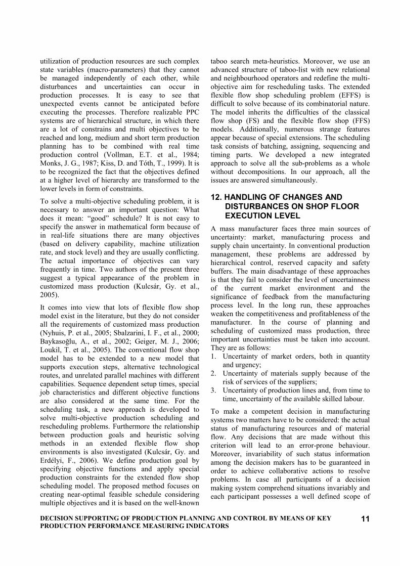
responsibility and boundaries of autonomy, the automation and synchronization of decision mechanisms can be achieved with high efficiency (Kulcsár, Gy. and Erdélyi, F. 2006). To achieve

advanced decision mechanisms in uncertainty the combination of Behaviour Based Control, BBC and Cockpit Task Management, CTM is addressed.

Model

Orders

Current

fine schedule

Scheduler

Simulation

Performance

Machines

Products

Routings

ERP Integrated scheduler and rescheduler

Uncertainty management

Cockpit task

Behaviour

Monitoring

Shop-floor

control

Production

processes

Tracking

MES

MES MES MES

Enterprise

Production

running program

Orders completed

engine

Evaluation

goals, situations

New constraints,

data basegenerator

evaluating

management

based control

State of machines

Figure 5 The structure of the integrated scheduling and manufacture control system

As we showed above stability of production is the fundamental requirement of manufacturing control policy (Tóth, T. and Erdélyi, F., 2006a; Tóth, T. and Erdélyi, F., 2006b).

One of the main control activities to remove production stability is the rescheduling action (Vieira, G. et al., 2003). Rescheduling is a process of updating an existing production schedule in response to disruptions or creating a new one if the current schedule has become infeasible. Rescheduling is a behaviour class of BBC based control.

Different type of uncertainty can occur i.e. machine failure or breakdown, missing material or components, under estimation of processing time, job priority or due date changes and so on. Different rescheduling methods can be used according to the effects of the unexpected events: time shift rescheduling, partial rescheduling or complete rescheduling. Time shift rescheduling postpones executions of certain tasks and jobs in time, but their resource assignments and sequences are not changed. Partial rescheduling modifies only jobs and resources affected by the disruption. Complete rescheduling generates a new feasible schedule. Our approach to solve rescheduling task is that we use multi-objective

searching algorithms similarly to the predictive scheduling. The aim of rescheduling is to find a schedule, which 1.) considers the modified circumstances, 2.) is near-optimal according to some predefined criterion and 3.) is as close as possible to the original one.

It is required of rescheduling methods to consider new demands that added to predictive scheduling problem. The last released schedule appears as a new input element of the rescheduling system and it is very important to preserve this initial schedule as much as possible to maintain the system stability. For this purpose, we defined qualitative indices (i.e. related to setup and due date) for supporting comparison of schedule changes.

13. CONCLUSIONS

In our research, we have analyzed the production goals in the Flow shop type production processes and the key performance indicators describing them. We have proved that the production goals are dependent on each other; therefore, their parameters cannot be improved at the same time.

We have worked out a new extended scheduling task class (Extended Flexible Flow Shop, EFFS) and its



computer representation for the modelling of production programming tasks at the workshop level, considering the general characteristics and requirements of mass production according to demand. The new extended model is characterized by the following:

At the same time they have: (1) machines (production lines) able to perform more than one operation together, (2) machine groups organized from parallel machines according to functions, (3) alternative implementation routes depending on the type of product, (4) production intensities depending on the machine and the product, (5) varying time periods of availability depending on the machine, (6) times for readjusting the machines depending on the sequence of jobs, (7) time limits on launching and finishing the jobs.

The new approach makes it possible to manage jobs dynamically, to merge and/or separate orders. This feature of the model provides a possible interpretation for the problem of lot size in mass production.

It is able to manage different optimization goals of varying importance, as well as interactive designer interventions in order to satisfy the flexibly changing demands of production control.

This scheduling software, based on a new concept, supports the solution of the rescheduling tasks for the management of manufacturing control and uncertainty at the MES level in cases where there is more than one production goal at the same time. It is an important feature of this application that it supports the user in the solution of scheduling and rescheduling tasks with an operation set providing consistent intervention at the level of orders, jobs, tasks and machines.

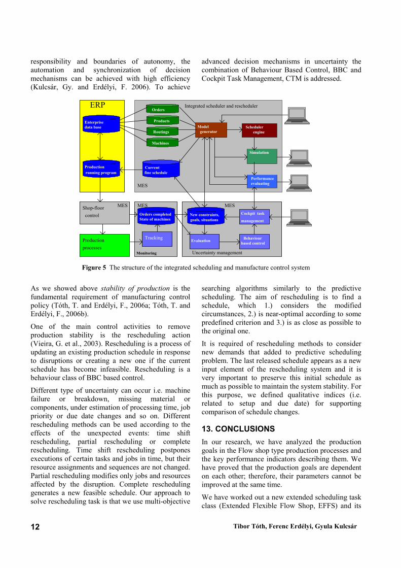
Table 1 consists of numerical results of a running test generated by the EFFS-PS application system. (Software designer: Kulcsár, Gy.) The input data base originated from a large Hungarian company being present in the consumer goods market.

Table 1 Numerical results of the EFFS-PS software in the case of a practical application

I M O J JL TMT TTΣ tms N Fur Fq

JT SPE Tp

1. 119 393 2173 3 14 33 1119 1052.60 0.3684 5.27 542.04 true 2m 20s

2. 56 424 2360 60 302 7183 1677 1128.37 0.5524 2.55 801.81 true 4m 8s

3. 58 371 2041 0 0 0 1613 1056.32 0.5094 2.48 834.81 true 2m 28s

4. 124 502 5231 4 58 27 2405 1986.08 0.3824 5.69 913.12 true 4m 42s

5. 40 151 1559 4 76 178 1581 759.97 0.5101 1.93 770.70 true 2m 18s

Notes: M – number of machines O – number of external orders J – number of jobs

LJ – number of late jobs

MTT – maximum tardiness

TTΣ – sum of tardiness

mst – maximum completion time - makespan

N – average number of jobs in the system (WIP level)

JT – average flow time (throughput time) of jobs

Fu – average machine utilization rate in the system

Fq – average production rate

SPE – satisfaction of the Production Equation

pT – EFFS-PS software processing time.

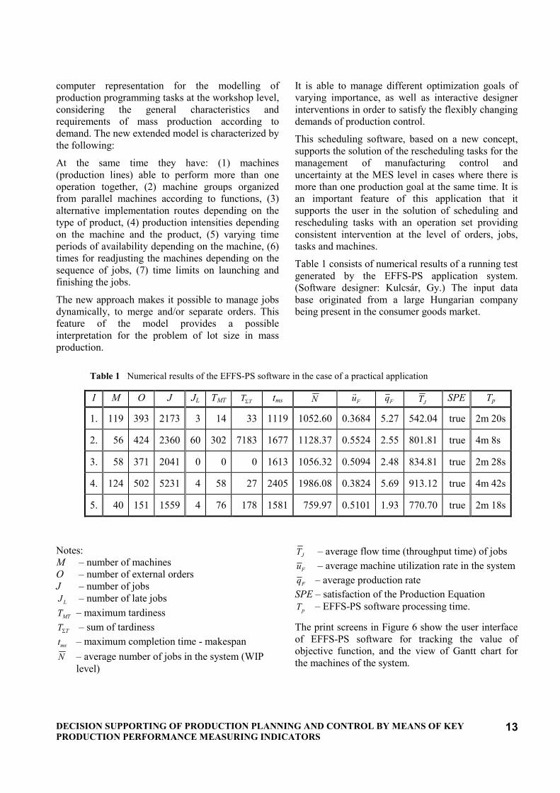
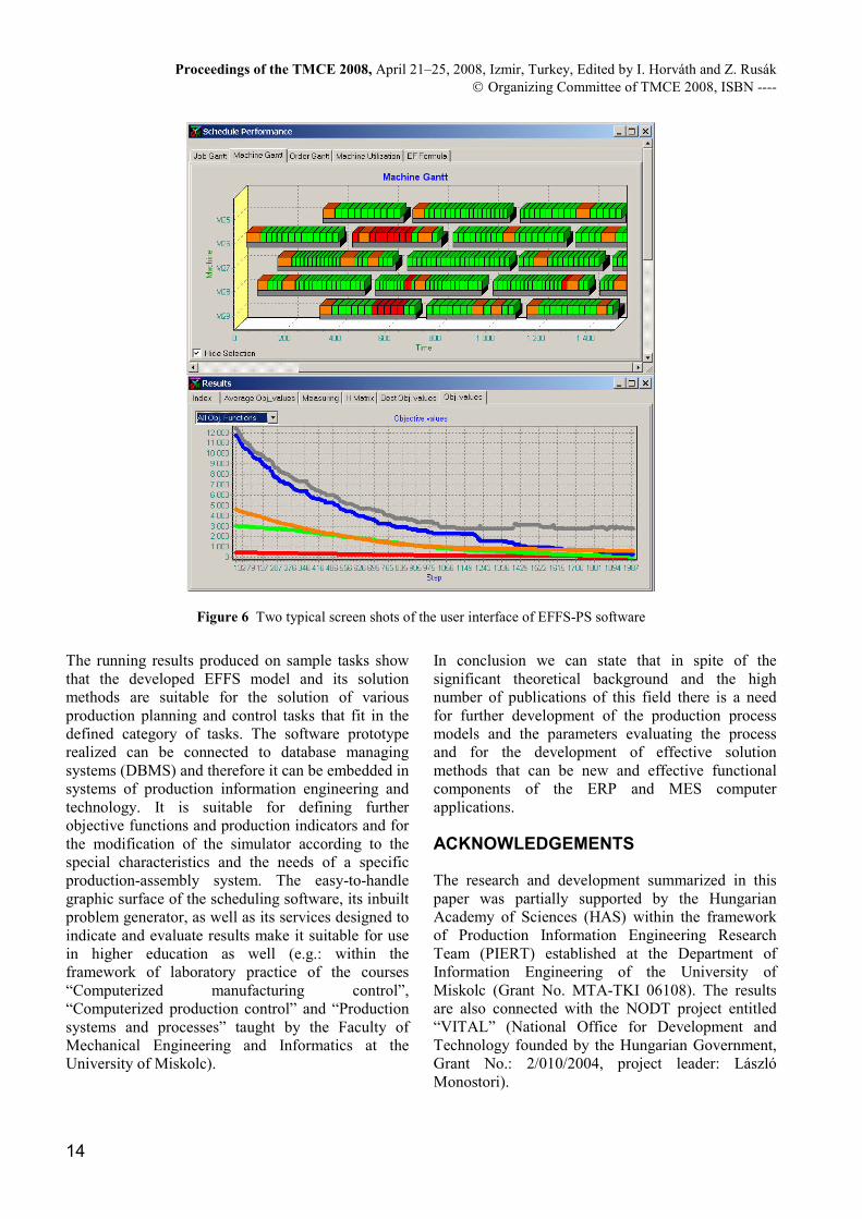
The print screens in Figure 6 show the user interface of EFFS-PS software for tracking the value of objective function, and the view of Gantt chart for the machines of the system.


14

Figure 6 Two typical screen shots of the user interface of EFFS-PS software

The running results produced on sample tasks show that the developed EFFS model and its solution methods are suitable for the solution of various production planning and control tasks that fit in the defined category of tasks. The software prototype realized can be connected to database managing systems (DBMS) and therefore it can be embedded in systems of production information engineering and technology. It is suitable for defining further objective functions and production indicators and for the modification of the simulator according to the special characteristics and the needs of a specific production-assembly system. The easy-to-handle graphic surface of the scheduling software, its inbuilt problem generator, as well as its services designed to indicate and evaluate results make it suitable for use in higher education as well (e.g.: within the framework of laboratory practice of the courses “Computerized manufacturing control”, “Computerized production control” and “Production systems and processes” taught by the Faculty of Mechanical Engineering and Informatics at the University of Miskolc).

In conclusion we can state that in spite of the significant theoretical background and the high number of publications of this field there is a need for further development of the production process models and the parameters evaluating the process and for the development of effective solution methods that can be new and effective functional components of the ERP and MES computer applications.

ACKNOWLEDGEMENTS

The research and development summarized in this paper was partially supported by the Hungarian Academy of Sciences (HAS) within the framework of Production Information Engineering Research Team (PIERT) established at the Department of Information Engineering of the University of Miskolc (Grant No. MTA-TKI 06108). The results are also connected with the NODT project entitled “VITAL” (National Office for Development and Technology founded by the Hungarian Government, Grant No.: 2/010/2004, project leader: László Monostori).



REFERENCES

Askin, R. G., Standridge, C. R. (1993), “Modeling and Analysis of Manufacturing Systems”. J. Wiley Inc. New York.

Baker, K. R. (1974), “Introduction to Sequencing and Scheduling”, Wiley. New York.

Bauer, Bowden, Browne, Duggan and Lyons (1991), “Shop Floor Control Systems - from design to implementation”, Chapman & Hall, UK.

Baykasoğlu, A., Özbakir, L., Dereli, T. (2002), “Dispatching Rule Based Heuristic for Multi-Objective Scheduling of Job Shops Using Tabu Search”, Proceedings of the 5th International Conference on Managing Innovations in Manufacturing, Milwaukee, USA, pp. 396-402.

Buzacott, J. A., Shanthikumar, J. G. (1993), “Stochastic Models of Manufacturing Systems”, Prentice Hall. Englewood Cliffs.

Ehrgott, M. (2000), “Multicriteria Optimization”, Springer, Berlin, etc.

Erdélyi, F., Tóth, T. (2004), “Production Planning of Individual Machine Systems: a Rate Based Approach Using Similarity”, Proceedings of the TMCE 2004. Lousanne, pp. 1133-1135.

Geiger, M. J. (2006), “Foundations of the Pareto Iterated Local Search Metaheuristic”, Proceedings of the 18th International Conference on Multiple Criteria Decision Making, Chania, Greece.

Goldratt, E. M. (1994), “Theory of Constraints”, North River Press, New York.

Kiss, D. and Tóth, T. (1999), “The methods of theoretical approach in Production Planning and Control. In: Information Systems for Enterprise Management in Hungary”, (Hetyei, J., Ed.), Computer Books, Budapest, pp. 59-94. (in Hungarian).

Kis, T. (2005), “Automatic Scheduling System with Basic Scheduling Engine”. For GE lighting. Specification. V. 06. VITAL project Cluster 1.

Krajewski, J., Ritzman, B. (1996), “Operation Management”, (Strategy and analysis), Addison-Wesley Publishing Co. New York.

Kulcsár, Gy., Hornyák, O., Erdélyi, F. (2005), “Shop Floor Decision Supporting and MES Functions in Customized Mass Production”, Machine Engineering, Vol. 5. Wroclaw, Poland, pp. 138 – 152.

Kulcsár, Gy., Erdélyi, F. (2006), “Modeling and Solving of the Extended Flexible Flow Shop Scheduling Problem”, Production Systems and Information Engineering, A Publication of the University of Miskolc, Vol. 3, Miskolc, Hungary, pp. 121-139.

Kulcsár, Gy., Erdélyi, F., Hornyák, O. (2007), “Multi-Objective Optimization and Heuristic Approaches for Solving Scheduling Problems”, IFAC Workshop, MIM 2007, Budapest, pp. 127-132.

Loukil, T., Teghem, J., Tuyttens, D. (2005), “Solving Multi-Objective Production Scheduling Problems Using Metaheuristics”, European Journal of Operational Research, 161, pp. 42-61.

Mckay, K. N., Wiers, V. C. (1999), “Unifying the Theory and Practice of Production Scheduling”, Journal of Manufacturing Systems, Vol. 18, No. 4, pp. 241-248.

Monks, J. G. (1987), “Operations Management: Theory and Problems”, McGraw Hill Book Company, New York.

Monostori, L., Váncza, J., Kis, T., Kádár, B., Viharos, Zs. (2006), “Real-time Cooperative Enterprises”, MITIP Conference, Budapest, pp. 1-8.

Nyhuis, P., von Cieminski, G., Fischer, A. (2005), „Applying Simulation and Analytical Models for Logistic Performance Prediction”, CIRP Annals, Vol. 54/1, pp. 417-422.

Papadopoulos, H. T., Heavey, C., Browne, J. (1993), “Queuing Theory in Manufacturing Systems”, Chapman & Hall, London, UK.

Sbalzarini, I. F., Müller, S., Koumoutsakos, P. (2000), “Multiobjective Optimization Using Evolutionary Algorithms”, Center of Turbulence Research, Proceedings of the Summer Program, pp. 63-74.

Scheer, A. W. (1994), “Computer Integrated Manufacturing”, Toward the Factory of the Future. Springer Verlag, Berlin.

Tóth, T., Erdélyi, F. (2006), “New Consideration of Production Performance Management for Discrete Manufacturing System”, MITIP Conference, pp. 435-444.

Tóth, T., Erdélyi, F. (2006), “Decision Supporting of Production Planning and Control by Means of Rate Type State Variables on the Basis of performance Indices of Production Triangle”, Proceedings of the TMCE 2006. Ljubljana, pp. 797-813.

Vernadat, F. B. (1996), “Enterprise Modeling and Integration”, Chapman and Hall. London.

Vieira, G., Hermann, J., Lin, E. (2003), “Rescheduling Manufacturing Systems: A Framework of Strategies, Policies and Methods”, Journal of Scheduling, Vol. 6, No. 1, pp. 35-58.

Vollman, E. T., Berry, W. L. (1984), “Manufacturing Planning and Control System”, IRWIN PC. Illinois.

decision supporting of production planning and...

Documents