decision analysis models for aircraft engine maintenance
TRANSCRIPT

Decision Analysis Models for Aircraft Engine
Maintenance Planning Using Discrete Event Simulation
by
Behnam Razavi
B.Sc., Mechanical Engineering, University of Saskatchewan, 2007
M.A.Sc., Mechanical Engineering, The University of British Columbia, 2009
A THESIS SUBMITTED IN PARTIAL FULFILLMENT
OF THE REQUIREMENTS FOR THE DEGREE OF
DOCTOR OF PHILOSOPHY
in
THE FACULTY OF GRADUATE AND POSTDOCTORAL STUDIES
(Mechanical Engineering)
The University of British Columbia
(Vancouver)
March 2015
© Behnam Razavi, 2015

Abstract
With stringent standards for materials, manufacturing, operation, and quality control, jet
engines in use on commercial aircraft are very reliable. It is not uncommon for engines to
operate for thousands of hours before being scheduled for inspection, service or repair.
However, due to required maintenance and unexpected failures aircraft must be
periodically grounded and their engines attended to. The tasks of maintenance and repair
without optimal planning can be costly and result in prolonged maintenance times,
reduced availability and possible flight delays. These factors have a negative impact on
both the airline operators and the passengers alike. Aircraft manufacturers and
maintainers, who provide after sale services, see significant benefits in constantly
improving health management and maintenance practices by deploying the most effective
maintenance strategies. Maintenance is seen as an imposed cost that ought to be
minimized. Airlines must evaluate new technologies and their possible role in reducing
the long term expenditure for operating a fleet of aircraft throughout its life cycle. A
significant share of these expenses goes towards maintenance of these aircraft, especially
their engines.
This study presents a model-based integrated decision making system for aircraft
engine maintenance planning. The goal is to determine the optimum number of engines
on an aircraft for maintenance based on logged engine operation data in order to
maximize the use of estimated remaining time to the next service as well as to minimize
ii

the duration of downtime. To achieve this, engine condition is used in a set of
preliminary Discrete Event Simulation (DES) models to evaluate and provide the most
effective maintenance policies for the aircraft engines. To assess options for making
decisions, a comprehensive model is developed based on the integration of the smaller
preliminary maintenance models for one, two, three and four engine maintenance cases.
Results from these analyses determine the optimal number of engines tagged for
maintenance on any aircraft in the fleet that arrives at the service facility. Since the
materials, technicians and other costs are proprietary information, this study is time-based
but allowance is made for the user to include associated costs and thus perform cost-
based decision making.
iii

Preface
This thesis entitled “Decision Analysis Models for Aircraft Engine Maintenance Planning
Using Discrete Event Simulation” presents the research performed by Behnam Razavi.
The research conducted in this thesis was supervised by Dr. Farrokh Sassani. The
following are the publications that have resulted from this thesis [7, 46].
• Behnam Razavi and Farrokh Sassani, 2013, "Aircraft Fleet Maintenance
Planning Using Combined Cost Benefit Model and Branch and Bound",
ASME International Mechanical Engineering Congress and Exposition,
IMECE, San Diego, CA, USA. This paper presents a maintenance planning
method for determining the time of maintenance based on the historical engine
operation data. Data from each engine with most chance of failure is then selected
and fed into an extended Branch and Bound (B&B) routine to determine the best
optimum sequence for entering the facility in order to minimize the waiting time.
The author of this thesis was the principal researcher of this publication. Dr.
Farrokh Sassani assisted with formulating the initial problem, and with writing
and editing the manuscript.
• Behnam Razavi and Farrokh Sassani, 2014, "Optimal Aircraft Engine
Maintenance Planning Using Discrete Event Simulation", Department of
Chemical & Biological Engineering, Research Day, October 1, University of
British Columbia, Vancouver, Canada. This was a poster which illustrated the
iv

overall maintenance planning and decision making procedure proposed for
Integrated Scenario Selection (ISS). The model developed and simulated in
Arena® discrete event simulation. Results reported in this poster are from the
material presented in chapters 2 and 4. Dr. Farrokh Sassani assisted with
modeling the problem and preparing the poster.
• Behnam Razavi and Farrokh Sassani, 2015, "Decision Analysis Model for
Optimal Aircraft Engine Maintenance Policies Using Discrete Event
Simulation". Integrated Systems: Innovations and Applications. In Press:
Springer - Verlag Berlin Heidelberg. This manuscript presents the development
of Discrete Event Simulation (DES) models that utilize aircraft flying, grounding
and engines service times, Time-On-Wing (TOW) data for each engine since its
last service, and Remaining-Time-to-Fly (RTTF) to aid optimal maintenance
policy decision making. The proposed models and techniques are explained and
discussed in chapters 3 and 4. The author of this thesis was the principal
researcher of this work. Dr. Farrokh Sassani assisted with modeling the problem,
and with writing and editing the manuscript.
v

Table of Contents
Abstract .............................................................................................................................. ii Preface ............................................................................................................................... iv Table of Contents ............................................................................................................. vi List of Tables .................................................................................................................... ix List of Figures .................................................................................................................... x List of Symbols ................................................................................................................ xii Glossary .......................................................................................................................... xiii Acknowledgements ........................................................................................................ xiv Dedication ........................................................................................................................ xv Chapter 1: Introduction ................................................................................................... 1
1.1 Preliminary Remarks ............................................................................................ 1
1.2 Impact of Maintenance ......................................................................................... 2
1.3 Maintenance and Aircraft Industries .................................................................... 6
1.4 Research Objectives ............................................................................................. 9 1.4.1 Aircraft Overhaul Planning ......................................................................... 10
1.5 Organization of the Thesis ................................................................................. 12
Chapter 2: Maintenance Opportunities and Planning ................................................ 14 2.1 Introduction ........................................................................................................ 14 2.2 Condition Inspection .......................................................................................... 15
2.3 Condition Based Maintenance (CBM) ............................................................... 16
2.4 Problem Description ........................................................................................... 18
2.5 Simulation Based Maintenance Policy Development ........................................ 21
2.6 Scheduling and Sequencing Methods of Arrivals .............................................. 25
2.6.1 Lowest Attribute Value (LAV) ................................................................... 25
2.6.2 First-In-First-Out (FIFO) ............................................................................ 25
Chapter 3: Discrete Event Modeling and Simulation .................................................. 26 3.1 Introduction ........................................................................................................ 26
vi

3.2 Simulation .......................................................................................................... 27
3.2.1 Simulation Benefits and Disadvantages...................................................... 28
3.2.2 Simulation Modeling Phases....................................................................... 29
3.3 Arena® Based Discrete Event Simulation .......................................................... 32
3.3.1 Simulation Components in Arena® ............................................................. 34
3.4 Arena® and Aircraft Maintenance Planning ....................................................... 37
3.4.1 Maintenance Model Development .............................................................. 41
3.5 Building the Models ........................................................................................... 44
3.5.1 1-Engine Maintenance ................................................................................ 47
3.5.2 2-Engine Maintenance ................................................................................ 48
3.5.3 3-Engine Maintenance ................................................................................ 49
3.5.4 4-Engine Maintenance ................................................................................ 50
3.5.5 Integrated Scenario Selection (ISS) Engine Maintenance .......................... 51
Chapter 4: Engines Maintenance Planning and Discrete Event Simulation Analysis .. 55
4.1 Introduction ........................................................................................................ 55 4.2 Overview of Engine Maintenance Scenarios ..................................................... 56
4.2.1 Maintenance Scenarios with a Fixed Number of Engines .......................... 57
4.2.2 Integrated Scenario Selection (ISS) Maintenance ...................................... 59
4.3 Arena® Simulations ............................................................................................ 60
4.3.1 Individual Maintenance Scenarios .............................................................. 60
4.3.2 Integrated Scenario Selection (ISS) ............................................................ 69
4.4 Model Verification for Individual Engine Maintenance Scenarios Using Simio Discrete Event Simulation .................................................................................... 79
4.4.1 Simio Discrete Event Simulation ................................................................ 79
4.4.2 Building the Models in Simio ..................................................................... 80
4.4.3 Simulation Stability .................................................................................... 83
4.4.4 Verification ................................................................................................. 83
4.4.5 Discussions and Conclusions ...................................................................... 86
Chapter 5: Alternative Decision Support System Using Queuing Theory ................ 88 5.1 Introduction ........................................................................................................ 88
5.2 Waiting-Line Analysis of Maintenance Facility ................................................ 89
vii

5.2.1 Arrival Distribution ..................................................................................... 91
5.2.2 Service Time Distribution ........................................................................... 93
5.2.3 Queue Discipline ......................................................................................... 94
5.3 The Multi-Channel Waiting-Line Model ........................................................... 94
5.3.1 Queuing Parameters .................................................................................... 96
5.4 Analysis of the Single-Line, Two-channel Waiting-Line .................................. 97
Chapter 6: Conclusions and Future Work ................................................................. 101 6.1 Summary .......................................................................................................... 101 6.2 Discussions ....................................................................................................... 102
6.3 Conclusions ...................................................................................................... 103
6.4 Suggestions for Future Work ........................................................................... 104
Bibliography .................................................................................................................. 105 Appendix A: Individual Scenarios Steady State Graphs .......................................... 122 Appendix B: ISS Maintenance Steady State Graphs................................................. 125
viii

List of Tables
Table 4.1: Number of Times Each Aircraft Visits the Service Facility – Part 1 .............. 63
Table 4.2: Number of Times Each Aircraft Visits the Service Facility – Part 2 .............. 64
Table 4.3: Preliminary Simulation Results for Individual Maintenance Scenarios .......... 65
Table 4.4: Simulation Results for Individual Maintenance Scenarios – Part 1 ................ 67
Table 4.5: Average Time Values for Individual Maintenance Scenarios – Part 2 ........... 68
Table 4.6: Number of Times Each Aircraft Visits the Service Facility (ISS Scenario) ... 73
Table 4.7: Number of Different Service Type for Sample Selected Aircraft ................... 74
Table 4.8: ISS Engine Maintenance Policy Simulation Results – Part 1 .......................... 75
Table 4.9: ISS Engine Maintenance Policy Simulation Results – Part 2 .......................... 77
Table 4.10: Simulation Average Time Values for ISS ..................................................... 78
Table 4.11: Average Values from Simio Simulations ...................................................... 84
Table 4.12: Average Values from Arena® Simulations .................................................... 84
Table 4.13: Percentage Difference between Simio and Arena® Average Values ............. 85
Table 4.14: Total Time Values from Simio Simulations .................................................. 85
Table 4.15: Total Time Values from Arena® Simulations ................................................ 85
Table 4.16: Percentage Difference between Simio and Arena® Total Time Values ........ 86
Table 5.1: ISS Engine Maintenance Queuing Model Characteristics ............................... 98
Table 5.2: Comparison of Different ISS Models ............................................................ 100
ix

List of Figures
Figure 1.1: Component Failure Rate over Time ................................................................. 4
Figure 1.2: Graphical Representation of Maintenance Operation ...................................... 9
Figure 1.3: TOW Graph Representing Engine Deterioration ........................................... 11
Figure 2.1: Maintenance Categories [18] ............................................................................ 17
Figure 2.2: Engine Condition and Time-on-Wing Characteristics ................................... 20
Figure 2.3: Schematic Flow Chart of Problem Description .............................................. 23
Figure 2.4: Engine Maintenance Overhaul Process .......................................................... 24
Figure 3.1: Schematic Block Diagram of Simulation Process .......................................... 30
Figure 3.2: The Arena® Home Screen .............................................................................. 33
Figure 3.3: Graphical Representation of Maintenance Operation .................................... 39
Figure 3.4: Simulation Model for Engine Maintenance ................................................... 45
Figure 3.5: Block Diagram for 1-Engine Maintenance .................................................... 48
Figure 3.6: Block Diagram for 2-Engine Maintenance .................................................... 49
Figure 3.7: Block Diagram for 3-Engine Maintenance .................................................... 50
Figure 3.8: Block Diagram for 4-Engine Maintenance .................................................... 51
Figure 3.9: Block Diagram for ISS Engine Maintenance ................................................. 54
Figure 4.1: Maintenance Operation for “Fixed” Number of Engines ............................... 58
Figure 4.2: Graphical Representation of Maintenance Operation for ISS ........................ 59
Figure 4.3: Screenshot of the Entire Arena® 1-Engine System ........................................ 61
x

Figure 4.4: Screenshot of blocks: (a) Engine Selection for Maintenance, and (b) Service
of Engines ...................................................................................................... 61
Figure 4.5: Estimating Replication Number for Individual Scenarios ............................. 62
Figure 4.6: Estimating Replication Number Based on Waiting Time .............................. 70
Figure 4.7: Screenshot of the Entire Arena® ISS Model .................................................. 71
Figure 4.8: Screenshot of the Maintenance Decision Block ............................................. 72
Figure 4.9: Screenshot of the Statistical Data Collection Block ....................................... 72
Figure 4.10: Graphical Representation of a Simio Model ................................................ 81
Figure 4.11: Overall Maintenance Procedure Flow Diagram ........................................... 82
Figure 4.12: Estimating Replication Number for Individual Scenarios for Simio ........... 83
Figure 5.1: Examples of Waiting-Line Systems ............................................................... 91
Figure 5.2: Percentage of Aircraft Serviced in t Weeks or Less ....................................... 97
Figure 5.3: Probability of n Units in the System .............................................................. 99
Figure A.1: Average Grounding Time for Individual Scenarios .................................... 122
Figure A.2: Average Flying Time for Individual Scenarios ........................................... 123
Figure A.3: Average Service Time for Individual Scenarios ......................................... 123
Figure A.4: Average Waiting Time for Individual Scenarios ......................................... 124
Figure B.1: Average Grounding Time for ISS Scenario ................................................. 125
Figure B.2: Average Flying Time for ISS Scenario ....................................................... 126
Figure B.3: Average Service Time for ISS Scenario ...................................................... 126
Figure B.4: Average Queue Time for ISS Scenario ....................................................... 127
xi
List of Symbols
k Number of channels
L The average number of units in the system
Lq The average number of units waiting for service
P0 The probability that all k service channels are idle
Pn The probability of n units in the system
Pw The probability that an arriving unit must wait for service
W The average time a unit spends in the system (waiting + service)
Wq The average time a unit spends waiting for service
𝑥 Number of arrivals per unit of time
λ Average number of arrivals in a specific period of time
μ Average number of units serviced in a specific period of time
xii

Glossary
AHP Analytical Hierarchy Process
AI Artificial Intelligent
CBM Condition Based Maintenance
CM Corrective Maintenance
DEDS Discrete-Event Dynamic Systems
DES Discrete Event Simulation
FIFO First-In-First-Out
HMM Health Management and Maintenance
ISS Integrated Scenario Selection
LAV Lowest Attribute Value
MRO Maintenance, Repair and Overhaul
PM Preventive Maintenance
RTF Run To Failure
RTTF Remaining Time to Fly
TNOW Time Now (current clock in Simulation)
TOW Time-on-Wing
Trs1 Primary Threshold
Trs2 Secondary Threshold
xiii

Acknowledgements
This research project would not have been possible without the support of many people.
First and foremost, I offer my sincerest gratitude to my supervisor, Professor Farrokh
Sassani, who has supported me throughout my thesis with his patience and knowledge as
well as his encouragement, guidance, unconditional help and effort. Additionally, I would
like to express my sincere gratitude to Professor de Silva and Professor Dunbar, members
of my supervisory committee, for their support and guidance.
I would like to thank my colleagues at Process Automation and Robotics
Laboratory (PAR-LAB) for their friendship and invaluable assistance, notably Atefeh
Einafshar, Morteza Taiebat, and Abbas Hosseini and Dr. M. Karafi. Very special thanks
go to Soroush Sharifi and Hediyeh Tehrani for their assistance and input.
I would also like to acknowledge the sources of financial support for this research,
namely: Natural Sciences and Engineering Research Council (NSERC) of Canada,
CRIAQ (Consortium de Recherche et D’Innovation en Aerospatiale au Quebec), and
GlobVision Inc.
I cannot end without thanking my family, on whose constant encouragement and
love I have relied throughout my time finishing the work. Finally, I would like to thank
my father and mother who are the source of all greatness; brother, sister and brother-in-
law; Behrad, Behnaz and Hossein, for their everyday support, and my late sister,
Bahareh, whose thought will always be in my mind.
xiv

Dedication
I dedicate this work to my father, Dr. Jalil Razavi, who is the greatest role model and a
friend. He has taught me to work hard for the things I aspire to achieve in my life. He is
the source of my motivation and inspiration.
“Success is about dedication. You need to have vision and think ahead which will lead
you to an incredible end”.
xv
Chapter 1: Introduction
1 Introduction
1.1 Preliminary Remarks
Measures are taken by many industries to keep machines and operating systems in
trouble-free condition and are collectively termed maintenance engineering. After an
equipment is designed, fabricated, installed and gained an operational status, it is the duty
of maintenance department to look after the health of the system to make sure it has the
operational availability. A system which is properly maintained and serviced during its
entire life cycle, in an ideal case, will reach its maximum availability. An engine on an
aircraft and holistically a fleet of aircraft is no exception. Considering the scale and scope
of the operation of a fleet, the associated times, costs and consequences of inefficient
maintenance can be very significant [1].
1
In regards to the traditional viewpoint, maintenance is required to repair and fix
the worn or damaged components of a system triggered by extended use or failure. A
more recent view of maintenance is defined in [2] as “all activities aimed at keeping an
equipment in or restoring it to the physical state considered necessary for the fulfilment
of its intended function”. Viewing this in a bigger scope, some more practical operations
could be included such as routine servicing and periodic inspections, preventive
replacement and condition monitoring. For instance, to improve engine reliability,
decisions could be made for component replacement (maintenance) or make some
positive modification to a design (fabrication). Therefore, in order to properly manage
maintenance, it should cover every stage in the life cycle including component
specification, data acquisition, planning, operation, and performance evaluation.
1.2 Impact of Maintenance
Maintenance is one of the tools for ensuring satisfactory system reliability. At a time,
however, when this approach is constrained, the mechanical components are forced to get
the most out of the system through more effective operating policies, including improved
maintenance programs. In fact, maintenance is becoming an important part of the
operation of any system. The implementation of effective maintenance programs can
represent a significant step in the direction of “getting the most out” of the equipment
installed. Monitoring the operating condition of equipment and their components has
recently been facilitated by means of developing computer-based maintenance planning
for better precision and accuracy; and thus effective cost reducing techniques.
2

Maintenance costs are usually a major portion of the total operating costs in most
operations [3, 4].
The concept of maintenance comes with the idea that it can be planned and
managed in such a way that it provides an efficient continuous operating conditions at all
times. In addition, the maintenance can be treated as an investment rather than a cost
cumulative procedure. The need for maintenance can be predicated before an actual
failure and ideally, maintenance is performed to keep equipment and systems running
efficiently for at least the designed life of the component(s). As such, the practical
operation of a component is a time-based function. If one were to graph the failure rate of
a component population versus time, it is likely the graph would take the “bathtub”
shape, as illustrated in Figure 1.1. In this figure the vertical and horizontal axes represent
the failure rate and time, respectively. From its shape, the curve can be divided into three
distinct: early failure, useful life, and wear-out periods [5].
The initial region that begins at time zero characterizes a high but rapidly
decreasing failure rate. This region is known as the early failure period. This period
typically lasts several weeks to a few months depending on the case. Next, the failure rate
stabilizes and remains roughly constant for the majority of the useful life of the
component. This long period of a constant failure rate is known as the the useful life
period. Most systems spend much of their lifetime operating in this flat portion of the
bathtub curve. Finally, if the product remains in use long enough, the failure rate begins
to increase as materials wear out and degradation failures occur at an increasing rate. This
is the wear-out failure period.
3

Fa
ilure
Rat
e
Time
Wear-outFailure
Constant (Random) Failure
Observed Failure Rate
Decreasing FailureRate
Constant FailureRate
Increasing FailureRate
Early Failure
Figure 1.1: Component Failure Rate over Time
When a system breaks down, it needs to be properly attended to in order to bring
it back to its normal operation. This conventional maintenance management philosophy is
categorized into two types: Run-to-Failure (RTF) and Preventive Maintenance (PM) [3].
The logic of RTF management is simple. As the name implies when an equipment
or a machine breaks down, repair it. This “if it is not broken, do not fix it” method has
been a major part of maintenance operations for long time. The RTF concept waits for
system failure before any maintenance action is taken. No capital or effort is spent until
the system fails to operate normally and requires attendance and repair. This in fact is a
4
most expensive method of maintenance management with many disadvantages. For
instance, a system at any time must anticipate a sudden failure and have the capability to
react in order to overcome consequences. It is indeed unimaginable, unlikely and legally
forbidden that one could use this technique for aircraft maintenance operation which in
case of a sudden failure will have catastrophic ramifications.
All preventive maintenance management programs are time driven or in other
words the maintenance is based on the number of hours of operation. As shown in Figure
1.1, the probability of a failure is more likely at the beginning of the operation. The
probability of failure decreases and then increases as the time passes and the normal life
operation period ends. Preventive maintenance is scheduling on a pre-determined interval
on the basis of statistics and knowledge of historical data. In general, it can be defined as
actions performed on a time based schedule that prevent degradation of a component or
equipment with the aim of extending system useful life time through controlling
degradation to an acceptable level.
While preventive maintenance is not the optimum maintenance program, it does
have several advantages. By performing the preventive maintenance, the life of the
equipment is extended. This translates into dollar savings. However, PM could be costly
if the failure occurs sooner than the system is scheduled for maintenance. As a result,
RTF type maintenance may be implemented and this will be even more costly than the
same repair made on a schedule basis. Preventive maintenance will generally run the
equipment more efficiently, reduce the probability and the number of failures.
Minimizing failures translate into maintenance and capital cost savings [5].
5

1.3 Maintenance and Aircraft Industries
Aviation maintenance activities are the backbone of all successful aviation industries.
Good maintenance provides safer and more reliable aircraft. It increases aircraft usage,
and provides confidence of air travel to the thousands or millions of travelers who want
to enjoy the safety of modern aircraft and transportation. A good maintenance
management is an asset that can provide the aviation industry the essentials necessary to
establish flying confidence in the public. Without having such good maintenance in
place, aviation industries can suffer severely if travelers face delays and cancellations,
and lose confidence in certain airlines for instance [6].
Any engine is prone to failure; however, properly maintained aircraft engines
could reduce the occurrence of failures. Therefore, aircraft manufacturers and users will
generally benefit from implementing Health Management and Maintenance (HMM)
techniques by developing effective maintenance planning and strategies. The goal of
HMM techniques is to reduce the life cycle costs for operating the entire aircraft fleet.
Considerable shares of these life cycle costs are expenditures for Maintenance, Repair
and Overhaul (MRO) of the individual aircraft engines [7].
The mechanical complexity of aircraft engines results in considerable labour
working hours for MRO related tasks such as disassembly, inspection and replacement of
expensive worn parts, reassembly and re-commissioning [8]. Therefore, engine MRO is
considered as a cost driver and it is in the interest of aircraft operators to estimate the life
cycle and the costs when making decisions regarding their aircraft fleet.
6

Moving forward from conventional maintenance strategies, at the present time the
newly formed maintenance operations are categorized into three types of maintenance
strategies: 1) Corrective maintenance in which the system is partially or completely shut
down and one or more of the components are replaced. However, the system condition
may not become as good as new. 2) Preventive maintenance which is performed based on
a predetermined interval. It aims to prevent problems associated with corrective
maintenance and to reduce system downtime. 3) Condition Based Maintenance (CBM) is
a form of preventive maintenance but is scheduled and performed based on the ‘live’
knowledge of the condition of the system components [9, 10].
Maity et al. [11] studied an automated scheduling model that took CBM into
account along with traditional preventive maintenance guidelines and used the
information such as part and facility availability, to arrive at an optimum maintenance
schedule. The model used Generic Constraint Development Environment (Gecode
software) alongside multiple constraints such as ordering of parts and crew availabilities.
Two issues, namely improving efficiency and reducing cost were treated.
Halasz et al. [12] put into practice an integrated system of remote monitoring and
decision support for a fleet of aircraft. An Artificial Intelligence (AI) program was used
to remotely monitor a fleet of commercial aircraft and alert maintenance staff in advance
to deal with an expected difficulty or fault which could disrupt the operation. One of the
main requirements for the system was to have vast information base such as a
communication network, document delivery and equipment dispatch regulations. The
7

system is yet to be implemented and tested against a real system and further improvement
is required such as maintenance cost evaluation.
Yanqing and Xueyan [13] developed an Analytical Hierarchy Process (AHP) to
tackle uncertainty factors in the process of aircraft safety risk management. Using AHP,
the priority weights of factors that affect aircraft flying safety was calculated. AHP both
assessed the safety and identified the hazards during the aviation maintenance in order to
improve the safety level. The degree of success in this study was dependent upon the
amount of information the aviation industry share with the authors and level of
uncertainty during the maintenance. Rad et al. [14] studied the effect of spare part
availability, their effect on maintenance planning, negative cost impact on flight
cancellation and airline performance. They used the available operational information in
Analytical Hierarchy Process (AHP) to classify the importance of the spare parts, usage
rate, unit price and reliability. The drawback for using AHP in this study was the
unavailability of such information.
Altuger and Chassapis [15] developed an Arena® based discrete event simulation
model for a decision making to select a PM scheduling plan for a manufacturing process
that gave the best utility and performance. Based on desired preferences, different criteria
with different confidence intervals were considered to evaluate and to assess the available
preventive maintenance schedules. They showed the advantages of discrete event
simulation in emulating real scenarios.
8

1.4 Research Objectives
Figure 1.2 shows the overview of the maintenance related operations envisaged for a fleet
of aircraft, where research activities within each box are conducted by a different group
of researchers. The arrows indicate the information flow. The research conducted within
the dashed-line box is the scope of the present thesis. Essentially, the in-flight monitoring
information is passed to the Diagnosis and Prognosis Group which then forwards its
analysis results to the Operations and Maintenance Task Planning Group.
Diagnosis and Prognosis
Operation and Maintenance Task Planning using CBM
Maintenance Resource Scheduling
Maintenance Decision Making
Scheduling and Planning
{{
Overhaul Time
Analysis
Aircraft Engine
Fleet of Aircraft
Figure 1.2: Graphical Representation of Maintenance Operation
9

The research objectives within this group (the present thesis) were to:
1- Model and evaluate various CBM engine maintenance policies for a fleet of
aircraft aiming to maximize the estimated remaining useful time to the next
service and minimize the duration of downtime.
2- Provide management and maintenance personnel with a simple decision making
tool to readily examine other alternatives and variations to the existing policies.
1.4.1 Aircraft Overhaul Planning
As engines on an aircraft are generally at different state of health, it is often one engine
that initiates the need for maintenance. However, an analysis is performed to see while
the aircraft is at the service facility, whether it is cost- or time-effective to extend the
preventive maintenance to other engines of the aircraft, and if so determine the number of
engines so as to minimize the total time of the overhaul, which equally means maximize
the available flying time.
The objective of Maintenance, Repair and Overhaul (MRO) planning is to
estimate and to utilize the maximum remaining useful life of the system components,
improve safety, and reduce maintenance down times. To meet these objectives, studies
have discussed different approaches [16]. For MRO, industries usually consider a few
parameters when monitoring a system. In aircraft, each engine should have sufficient
performance margin time between repairs to carry it through to the next overhaul. Each
engine in the system is represented by its own Time-On-Wing (TOW) graph which
10

shows its condition over time, and from which the Remaining-Time-to-Fly (RTTF) value
can be estimated.
As shown in Figure 1.3, if the engine is close to the maximum certified operating
limit, it must be sent for overhaul. The goal is to safely identify any of the engines in
operation and place them for maintenance when their remaining flying time is near the
assigned typical threshold of 100 hours. However, there are no clear policies as to how
many of the engines should be attended to once an aircraft is grounded due to one engine.
Therefore, the aim of this study is to develop detailed simulation models where different
policies can be examined.
Maximum certified operating limit
100 hours
Latest Time for
CBM
Deterioration margin
Time-On-Wing (hrs)
Engi
ne C
ondi
tion
{
CorrectiveMaintenance
Bad
Good
Figure 1.3: TOW Graph Representing Engine Deterioration
One of the main challenges associated with this study was its confidentiality
issues related to the release of information by the company involved. Due to the
11

proprietary information, the simulation model developed is based on synthetic data. The
verification of simulation model was achieved through simplified and alternative
modeling analysis. The industrial partner/user will undertake running the model with real
proprietary data in confidence once the working model is concluded.
The plan of study presented here is to develop aircraft engine maintenance scenario
analysis models using discrete event simulation for a fleet of aircraft. This is to help the
maintenance managers evaluate alternate policies and take the best course of action that
is most effective in reducing the grounding and service times. This maximizes the
availability of aircraft in the fleet. Since discrete event simulation requires deep
knowledge of discrete event modeling concept which have slow changing learning
curves, an extended plan is to re-cast the simulation results from the discrete event
modeling onto a “queuing concept modeling”. Queuing models can be represented in
mathematical equations that can be readily manipulated to assess many alternative
policies.
1.5 Organization of the Thesis
In Chapter 1, an introduction to a typical aircraft industry and the related current and
common maintenance schemes were introduced. Planning different methods of
maintenance, which has always been an essential part of any industry and has been a
major challenge for the aircraft industry, was brought into the forefront. Some of the
common difficulties that arise in obtaining optimal maintenance planning were discussed.
12

Next, a review of literature related to aircraft and maintenance was presented, and the
main objectives of the current research were outlined.
Finally, an overview of maintenance operation, and the basic concept of
Condition Based Maintenance (CBM) were graphically presented.
In Chapter 2, various forms of maintenance, specifically, CBM are introduced and
discussed in greater detail. As well, the overall problem statement under consideration is
explained.
The development of discrete event models and simulation that are relevant to the
current study are undertaken in Chapter 3. Specifically, Arena® based discrete event
simulation models with respect to aircraft engine maintenance planning is developed.
In Chapter 4, the simulations with the developed DES models for aircraft
maintenance are carried out. Results for the proposed methods of maintenance are shown,
followed by discussions on the outcome of the maintenance schemes. At the end, the
simulation results obtained using Arena® are verified against a parallel work developed
and implemented in SIMIO discrete event simulation software.
In Chapter 5, queuing theory is introduced and used based on both the existing
information from data logs and the results obtained from the discrete event simulations.
Chapter 6 draws conclusions from the modeling and simulation results of the
study. Recommendations are made on possible future work for improvement of the
developed techniques.
13

Chapter 2: Maintenance Opportunities and Planning
2 Maintenance Opportunities and Planning
2.1 Introduction
This chapter describes and discusses the overall project aim, the challenges associated
with this study and the current problems the aircraft industry face, and the methodologies
proposed in this study. As indicated in the previous chapter, the main focus of this
research is to obtain efficient and cost effective policies of maintenance which would
prolong the useful life of aircraft engines. An effective policy is one that allows aircraft to
have longer flying periods which in turn minimizes the downtime and maximizes the
overall profits. Achieving these objectives provides the aircraft industry/user a system
with an optimal performance and aircraft engine conditions which meet the desired and
regulatory criteria of being healthy and safe. The effort here is to develop Condition
14

Based Maintenance (CBM) plans and avoid un-timely costly repairs or Corrective
Maintenance (CM).
Condition inspection frequency and condition based maintenance and their
relations to component failure and deterioration are explained in section 2.2 and 2.3,
respectively. This is followed by the problem description and the main challenges
associated with this study in section 2.4.
In section 2.5, the proposed simulation based maintenance policy development
and related literature review are presented. Implementing different sequencing methods
of entity arrivals in the proposed maintenance system are discussed in section 2.6.
2.2 Condition Inspection
A major disadvantage of the time based/planned preventive maintenance is that
some useful life of the equipment that still remains is lost when earlier-than-needed
service is performed. However, taking into account the consequence of a failure, it is a
better option to use preventive rather than corrective maintenance. When dealing with
capital intensive systems, it is more logical to inspect them regularly before removing and
subjecting them to maintenance. Through this ‘condition monitoring’, a better
understanding of the system health can be achieved and maintenance performed in a
time-optimal fashion that allows longer uninterrupted in-operation periods for the system.
15

2.3 Condition Based Maintenance (CBM)
Every manufacturer or service company has a set of defined assets on which its
existence depends. Continuation and availability of these assets will ensure the business
productivity while it is in operation. In a large enterprise, reducing costs related to
maintenance, repair, and ultimate replacement is at the top of the management concerns.
Downtime in any industrial system ultimately results not only in high repair and other
costs, but also in customer dissatisfaction and lower potential income [17].
Figure 2.1 represents the common types of maintenance. In general, the concept
of maintenance is divided into unplanned and planned [18, 19]. Unplanned maintenance,
or sometimes referred to as reactive maintenance, is performed when a failure occurs in
the working system and it is required to restore the system to its original or near-original
condition. This restoration through maintenance is also referred to as corrective
maintenance. There are cases when an immediate action is required in order to avoid
hazardous situations. This urgent type of maintenance is sometimes referred to as
emergency maintenance. Planned maintenance, or so called proactive maintenance,
categorizes into: preventive maintenance or predictive maintenance. Kothamasu and
colleagues [18] investigated three types of preventive maintenance: constant interval, age
based and imperfect. Furthermore, they also investigated types of predictive maintenance
and they categorized it into Reliability Centered Maintenance (RCM) and Condition
Based Maintenance (CBM).
Maintaining processes and systems have evolved dramatically over the years.
Nowadays, effective maintenance systems are expected to detect early forms of
16

degradation in predictive maintenance practices using Condition Based Maintenance
(CBM). Basically, condition based maintenance is a methodology that combines
predictive and preventive maintenance with real-time monitoring. CBM detects faults and
identifies sources sufficiently ahead of likely failures. This characteristic makes this type
of maintenance a proactive process which acts in advance to deal with unexpected and
impending faults.
Figure 2.1: Maintenance Categories [18]
Actions that extend the life of equipment include: lubrication, cleaning, adjusting
and the replacement of numerous minor components like drive belts, gaskets, filters, etc.
Actions that prevent unnecessary failure include timely and consistent equipment
inspection, and an aggressive use of non-destructive testing techniques such as vibration
analysis, infrared testing, or in-system sensor-based techniques. Through the utilization
17

of various non-destructive testing and measuring techniques, predictive maintenance
significantly improves estimating equipment health status as well as the best time for
maintenance before costly repairs are required [20]. Thus through CBM, the time of
initiation of failures is predicted long before it occurs based on the knowledge from
system components [3, 20].
Al-Najjar and Alsyouf [21], Rosqvist et al. [22, 23], Waeyenbergh and Pintelon
[24, 25] and Wang et al. [26, 27] provided some insight into when a particular
maintenance technique should be employed. CBM and its advantages have been
discussed in many studies [19, 28-30]. However, with some exceptions, surprisingly
little attention has been paid to different aspects and types of condition based
maintenance. Jardine et al. [31, 32] provided an overview of different types of tasks
within a CBM program such as data acquisition, data processing and maintenance
decision making, algorithms and technologies for each task.
2.4 Problem Description
Nowadays, the actual life of an aircraft fleet is not the same as the expected life of the
original design. To a great extent, it is determined by the degree of maintenance, the
maintenance expenditure, and the economic considerations required for the fleet to
continue its operational requirements. Due to the development of health monitoring
technologies, Condition Based Maintenance (CBM) policies have become increasingly
suitable for application in areas such as aircraft industry. Engine health management,
18

engine life management and maintenance decision making are the primary content of an
engine CBM policy [10].
The problem in CBM and preventive maintenance arises when one tries to
examine the stored and collected engine performance data to gain knowledge of the
current condition, predict degradation trend curves, and to optimally determine the proper
maintenance times. This information is essential in order to best manage the estimation
and improve the engine life, provide spare parts, prevent fatal injuries, and to
substantially reduce the cost of operations and maintenance as a whole. However, due to
its physical construct, maintenance of a single engine by itself is a very involved task.
When this is compounded with the need to maintain a fleet of engines within many
stringent constraints and standards, the problem can become prohibitively large,
operationally inefficient and costly.
Development of a decision support scheme for an aircraft fleet is essential for
tracking individual engines within a fleet, and producing safe and cost-effective
maintenance plans. Implementing any technique that uses a large volume of monitoring
data with many operational details requires very precise and careful data mining,
interpretation, and modeling, before any useful application can be imagined. A small part
of this study involves analyzing health trend curves, or so called Time-on-Wing (TOW)
graphs, as a function of flying time for different engine models. Figure 2.2 elaborates on
TOW graph a single engine.
19

Figure 2.2: Engine Condition and Time-on-Wing Characteristics
The engine condition deteriorates as the number of flying hours increases.
Preventive maintenance (PM) is performed to improve engine condition and to maximize
its TOW operation before reaching the maximum certified operating limit or complete
failure of a component in which a costly removal-from-the-wing and corrective
maintenance (CM) must be performed. In CBM, the knowledge about the system
component will help correctly decide on the cycle of PM only when it is needed to reduce
unnecessary costs and maximize the profits.
The trend of these TOW graphs are expected to be non-linear, and will be updated
as new data become available to better estimate the time margin (remaining time) of safe
operation. As will be thoroughly explained in later sections, utilizing flight information
and system analysis techniques, such as Discrete Event Simulation (DES) modeling, will
help to investigate and to predict the engine overhaul needs and remaining TOW.
20
Each engine in the system is represented by its own TOW graph which shows its
condition over time, and from which the Remaining-Time-to-Fly (RTTF) value can be
estimated. The objective here is to develop a detailed DES model for a fleet of aircraft
which can examine different scenarios using identified engines with their RTTF near
assigned typical threshold of 100 hours of reaching maximum operating limit. DES can
assist the user in selecting suitable policies for minimizing downtime and maximizing
aircraft availability.
2.5 Simulation Based Maintenance Policy Development
Discrete event simulation has been suggested and used by many researchers for
development of system analysis and decision making tools as it allows numerous options
to be evaluated before the best scenario can be selected. Various researchers have
reported significant benefits from the use of simulation-based models for process
improvement, scheduling and scenario comparisons [6]. Some studies have used DES to
design efficient production and business systems, to validate alternatives and propose
solutions to improve performance, sales and profits [33, 33-35]. Other investigators have
used it for decision making in preventive maintenance scheduling, network behaviour and
personnel scheduling and maintenance operation for flight training department [15, 36-
38]. Different scheduling approaches for dynamic manufacturing shops and facilities, and
evaluating the performance and the profit of manufacturing systems are other examples
of the use of DES [39, 40].
21

In DES, the system status progression depends on the initiation and occurrence of
events at different times by different objects or entities. For example, in a fleet operation,
the arrival of an aircraft for maintenance is an event of interest, and its arrival time or
duration can be variable, depending on the current state of the system and the condition
of the engine. These kinds of systems, characterized by discrete variables and continuous
time, are called Discrete-Event Dynamic Systems (DEDS) [41]. The different methods
for modeling and simulation of DEDS are called discrete event modeling and simulation
[42]. Although time is continuous, discrete-event modeling and simulation assumes that
only a finite number of events can occur in a determined period. To this extent, a
discrete-event simulation can be very efficient since it only needs to represent the
changes of state as an event takes place, rather than continuously.
Health management technologies monitor systems and detect abnormal behaviour
and then relate it to useful information about the system's condition. When the condition
of a system, such as its degradation level, is continuously monitored, a Condition-Based
Maintenance (CBM) can be implemented [43-45].
As shown in Figure 2.3, condition data of each engine in the fleet is captured
using in-flight sensory systems. This information is received and used as an input in the
“engine RTTF analysis” block. In the time analysis block, some maintenance policies are
defined and implemented within the DES and the maintenance plan is decided upon
before any aircraft is dispatched to the service facility [46].
22

Maintenance Plan
Engine Condition
Maintenance Policies
Engines RTTF
Analysis
Resume Flying
Discrete Event
Simulation
S.2 S.1
S.3 S.4
Fleet
Aircraft
Service Facility
Figure 2.3: Schematic Flow Chart of Problem Description
When the status of ‘one’ of an aircraft’s engines is near its assigned threshold of
reaching maximum certified operating limit, a maintenance activity is assigned and the
aircraft is put into the maintenance planning system. Once the plan is set, an overall
overhaul time analysis is conducted to see whether it is beneficial to perform
maintenance on more engines, rather than on the ‘one’ that initiated the maintenance,
while the aircraft is grounded.
Inside the service facility there are four stages of maintenance activity for each
engine which are laid out in series as shown in Figure 2.4. The time it takes to perform
each stage is determined by the user based on the type of the engines on a specific
aircraft. Since this complete information is not available due to confidentiality, based on
limited information made available, approximate hypothetical/synthetic data will be
randomly generated and used in the simulations carried out in this study. Engine
23

diagnosis and disassembly, repair and maintenance, indoor assembly and partial testing,
and outdoor engine testing and release are the four tasks performed in series that are
designated by S.1, S.2, S.3 and S.4, respectively.
Diagnosis and Disassembly
(S.1)
Repair and Maintenance Task
(S.2)
Indoor Assembly and Partial Testing
(S.3)
Outdoor Testing and Release
(S.4)
Figure 2.4: Engine Maintenance Overhaul Process
In engine diagnosis and disassembly module, the engine is disassembled into parts
if necessary, and sent to part inspection module for cleaning, functionality assessment,
non-destructive testing, detecting cracks, and dimensional checks on blades and vanes,
for example. In Repair and maintenance module, parts are repaired or replaced and sent
for re-assembly and indoor partial testing. The next step is to complete the final stage of
the testing outdoor if needed, and discharge the engine. Once the engine is released,
engine status is updated and recorded as engine service history for future use and
reference.
24

2.6 Scheduling and Sequencing Methods of Arrivals
Scheduling deals with the planning of operations. The task is essentially the
‘placement for service’. Whereas sequencing concerns the maintenance facility where a
decision has to be made as to the priority of the services performed. In the DES models
developed in this work, two sequencing rules are implemented as described below.
2.6.1 Lowest Attribute Value (LAV)
The Low attribute value is used for the grounding of aircraft for maintenance.
(The term Attribute becomes clear when the Arena® concepts are described in Chapter 3.)
LAV is the natural and desirable choice since the aircraft closest to the assigned threshold
(lowest safe flying time remaining) aircraft must be grounded first. As such, it is enforced
by default in the modeling concepts used in this work.
2.6.2 First-In-First-Out (FIFO)
In the maintenance facility for the queue of aircraft, if there is no specific reason
to resort to a particular priority rule or a sequencing algorithm, the best heuristic rule that
minimizes ‘Mean Flow Time’ and the ‘Work-In-Progress’ is the ‘Shortest-Service-Time-
First’. Since, a maintenance facility is a dynamic system where there is constant arrival of
aircraft; such a policy can consistently disadvantage some aircraft waiting for service.
From commitment-to-return-to-particular-flying-route, and uniformity of maintenance
service provided, it was decided that it is both acceptable and ‘fair’ to use the convenient
and most practical ‘Fist-In-First-Out’ queue discipline [47-49].
25

Chapter 3: Discrete Event Modeling and Simulation
3 Discrete Event Modeling and Simulation
3.1 Introduction
Experimentation is still one of the principal methods of problem solving. However, when
problems are more complex and do not readily lend themselves to experimentation alone,
they must be tackled in some other ways. One solution to study such a problem
thoroughly is to divide it into smaller sub-problems and create feasible models that make
the solution and analysis possible [42]. Discrete event simulation software is a versatile
and powerful tool for modeling and investigating the performance of complex systems.
In this chapter, discrete event simulation, Arena® simulation software, modeling
concepts, and the simulation models developed in this study are presented.
26
The organization of the material in this chapter is as follows: simulation, its
benefits and disadvantages, and different phases involved in simulation modeling are
discussed in section 3.2. This is followed by an introduction of Arena® based discrete
event simulation for the maintenance system being studied in section 3.3. Application of
Arena® simulation in the present study is discussed in section 3.4 and model formulation
discussed in section 3.5.
3.2 Simulation
Discrete event modeling and simulation technique is intended to ‘copy’ a real-world
process or system and mimic its operation over time. To simulate, it first requires a model
to be developed. This model represents the key characteristics or functions of the selected
physical system or process. The model represents the system itself, whereas the
simulation represents the operation of the system over time [50] as events take place.
Each event occurs at a particular instant in time and marks a change of one state, and may
cause initiation of other (future) events in the model. As consecutive events take place in
the model and simulation advances in time from one event to the next, changes occur in
system states, and relevant statistics are collected. In the field of maintenance and
planning, many studies have been conducted using DES modeling [15, 34, 38, 39, 47, 51-
58].
Discrete event simulation has been identified as one of the most used techniques
in the area of operations management [59]. Simulation models have been applied to
maintenance [15, 60] to increase production output in the manufacturing systems. Roux
27

and colleagues [61] studied a new approach that combined optimization algorithms and
simulation methods in an effort to evaluate the performances of various maintenance
strategies for manufacturing systems. Oyarbide-Zubillaga [51] has opted to focus on the
preventive maintenance in the manufacturing field. His main objective was to find the
optimal frequencies for the preventive maintenance of multi-equipment systems using
cost and profit criteria.
3.2.1 Simulation Benefits and Disadvantages
There are many benefits as to why simulation is an appropriate tool as outlined in [62].
Some of these benefits are:
1. Simulation enables the study of internal interaction of a subsystem with the
complex parent system.
2. Informational, organizational and environmental changes can be modelled and
their effects studied.
3. A plan can be visualized with animated simulation.
4. Simulation can be used with new designs and policies before any implementation.
At the same time this tool can help to understand why certain phenomena occur in a
real system.
There are also reasons why simulation can sometimes be inappropriate:
1. Modeling is a costly process.
2. Simulation requires special training and most likely the models generated by
different modellers to represent a system of interest will be different.
28

3. It is sometimes difficult to know if a simulation output is a result of system
interrelationships or randomness as some simulation outputs are based entirely on
random inputs (i.e. random number generation). Therefore, if it is used, correct
interpretation of results is very important.
3.2.2 Simulation Modeling Phases
Modeling is the process of producing a replica that represents construction and working
of a system of interest. A model can be similar to but sometimes is simpler than the
system it represents. A model can be reconfigured and experimented as it is usually
expensive and sometimes impossible or impractical to implement changes in the actual
real system it represents. In a simulation study, human decision making is required,
namely, in model development, experiment design, output analysis, conclusion
formulation, and decision making [63, 64]. Experienced problem formulators, simulation
modellers and analysts are essential for a successful simulation study. Figure 3.1 shows
the steps used in modeling and simulation. These steps are described in detail below [42]:
1. Problem Formulation: this is the first step in the simulation process and begins with
understanding the problem in hand. In the case of an aircraft maintenance planning, it
is desired to develop new strategies to obtain cost effective maintenance plans to
minimize downtime. This stage requires understanding of the system’s operational
behaviour and the activities that take place within its framework. Based on the stated
criteria and constraints, acceptable concepts must be narrowed down.
29

Problem Formulation
Conceptual Modeling
Modeling
Simulation
Experimentation
Output Analysis Validation
Verification
Figure 3.1: Schematic Block Diagram of Simulation Process
2. Conceptual Model: in this stage, it is required to identify all the objects (entities) and
their characteristics (attributes) and to construct a high-level structural and
behavioural description of the system. State variables are needed to be defined, their
relationship and importance to the study needs to be justified. Essential elements,
most important system requirements, possible future changes and operational
environment are expressed and considered.
30

3. Modeling: in the modeling stage of simulation, on the basis of the defined objects,
their characteristics and system behaviour, building a detailed representation of the
system based on the conceptual model is undertaken. In the model any assumptions
related to the system simplification must be stated.
4. Simulation: in this phase, a proper programming language and tools must be used to
implement the model and run simulation for results.
5. Experimentation: once the conceptual model is set, simulation is then executed and
the result is revealed which is often a set of numbers. Simulations are often run
multiple times to obtain a range of results. The output must be evaluated to determine
the precision level of the built model.
6. Simulation Output Analysis: in this phase the analysis of the simulation output is
needed in order to understand the system behaviour. At this stage, visualization tools,
graphical representation of simulation outputs, can be used to help with the process.
The goal of visualization is to provide a deeper understanding of the real system
being investigated and to help explore the large set of numerical data produced by the
simulation. This phase can sometimes be combined with Experimentation stage in
which the output is revealed, for instance, in the form of statistical graphs or charts.
7. Verification and Validation: Verification ensures that the model correctly represents
the real system in terms of its elements, functions and events [65]. There are two
common ways of verification. One method is to use ‘specific inputs’ with known and
‘expected output’, and observe whether the model satisfies the expectations. The
other approach is to model the system using a secondary modeling means, such as a
31

simplified analytical method. Validation ensures that the model and simulation re-
produce output data very close to that of the real system. This gives confidence that a
model is a vey close representation of the real system, and any changes in the model
parameters will produce meaningful results. This however, is only possible when a
real system does indeed exist. Otherwise, a properly conducted verification is
assumed sufficient.
3.3 Arena® Based Discrete Event Simulation
Arena® is a high-level simulation software that functions through a graphical user
interface. This flexible and powerful tool can create simulation models which can
accurately represent a system. The entire graphical model development of a system is an
object-oriented design process. System components are built using graphical objects, or
modules, which are placed in the layout window. Once a graphical simulation model is
created, the Arena® simultaneously generates the underlying model in an executable code
which performs the actual simulation runs [66, 67]. The modeling structure it follows is
very similar to that of a flowchart style model building regardless of their modeling
complexity. It consists of many modeling features, or templates, that are designed for
many different types of applications.
Figure 3.2 represents the Arena® home screen with some explanation of its
components and features. The Arena® main template consists of a panel or a set of panels
that include modeling constructs for a particular application, system, class of systems, or
general target environment.
32

A template panel contains modules collected into a file and intended to be
presented as a self-contained group. The panels commonly used for standard Arena®
modeling include: Basic Process, Advanced Process, and Advanced Transfer [68].
Arena® modellers attach template panels to the Project Bar in the application window of
the Arena® modeling environment. The Project Bar hosts the primary objects used to
build a model, so the modeller selects modules from the appropriate Project Bar panel
and places them in the model window.
Template Panel
Animate Toolbar
Drawing Toolbar
Model Windows Flowchart View
Project Bar Toolbar
View Toolbar
Model Window Spreadsheet View
Menu Bar
Figure 3.2: The Arena® Home Screen
33

Liu et al. [69] used Arena® based DES in their study of personnel planning for
materials handling at a center for unloading cargo from an incoming trailer truck and
loading them directly onto outbound trucks. The implementation of their proposed
method in Arena® proved to be a powerful tool in assisting logistics managers in their
personnel planning. Shih and Chin [70] presented a model for parts distribution center
developed in Arena®, which aimed at providing information about the total time of the
retrieving process as the system was working under readily unpredictable demands. The
results obtained using simulations made the dynamic system more understandable for the
management. It was also used as a supporting tool to make decisions in estimating the
required number of employees for the retrieving process.
3.3.1 Simulation Components in Arena®
Different modeling components and constructs are used to build a working simulation
model. Some of the main components of Arena® are described in this section [71].
Entities
An ‘Entity’ refers to an object in the simulation that can move, change properties, and
carry information through model. What role it plays depends on what is being modelled
and what is intended by the model builder. As well, entities can be created at any time,
leave the simulation or keep circulating in the system. They can change status and affect
the performance measures, and can be affected by other entities and the state of the
system. Most entities represent real objects in a simulation and a model can consist of
different entities representing different objects.
34

Attributes
Each entity in simulation has both a specific characteristic and a value with which it
differentiate itself from another entity. It is up to the modeller to assign or to change
certain attribute of an entity when modeling a system. It is important to note that values
associated with attributes are only tied to specific entities. Another way of understanding
attributes is to think of them as tags attached to entities which reveal their characteristics.
Arena® automatically keeps track of attributes which are defined, value assigned to or
changed for the entities in the system. Examples of assigning attributes are the “time of
entrance” and “maintenance durations”.
Variables
Variables reflect system characteristics regardless of the number of entities in the system.
Variables are unique and a model may have many of them defined for the system of
interest. There are two different ways variables can be defined in Arena®, one is defined
by the modeller (user-defined variables) and the other is defined variables that already
exist (built-in variables). Unlike attributes, variables do not belong to a specific entity but
rather tied to the whole system. Any entity in the system can use the defined variables
and/or change them based on system specifications or operation.
Variables are used for many different purposes. For instance, the pre-defined
grounding time in this model is the same throughout and is called “threshold”. This
variable is set to an appropriate value and then used whenever this constant is needed. In
a modified model and investigation where this “threshold” is set to a different value (in
35

one place), it will be the same and available throughout the simulation for access and use
by all system entities.
Resources
Entities receive services from resources that could represent personnel, equipment or
space in a storage area of limited size. The resource is given or assigned to an entity when
it is available and needed. Commonly, it is said that the entity seizes the resource for an
activity and then releases it when the activity is completed. A resource can represent a
group of several individual task performers or servers who perform multiple tasks as
intended by the model developer. For instance, a repair facility can have few stations
where the staff amongst other activities, take a break based on a pre-defined schedule or
rules.
Queues
When an entity arrives for a service and the resource has already been seized by another
entity, it will have to form a line, or stay in a queue, until the resource is released. In
some models queues have a capacity assigned by the modeller and cannot accommodate
when the number of entities exceed that capacity. Various disciplines can be used at
queuing nodes such as First-In-First-Out, Last-In-First-Out and Priority.
Events
An event is a concept that occurs at an instant of time while the simulation is running and
that might change attributes or model variables. An example of an event is the arrival of
36

an entity or its departure. In this study, aircraft in queue leave the line and enter the
service facility which changes the system status, but this occurs because an end of service
event has occurred and another aircraft has left the facility and caused other changes. In
Arena® this information is stored in an event calendar using a simulation block called
record which stores all the information (schedule) for future events.
Simulation Clock
The simulation must keep track of the current simulation time, in a unit suitable for the
system being modeled. In discrete event simulations, the clock skips to the next event
start time as the simulation proceeds. In other words, unlike real time, the simulation
clock does not take on all values and it launches from the time of one event to the time of
the next event.
Starting and Stopping
Another task in a simulation is to plan its start and stop times. The modeller must
determine the appropriate starting condition, how long a run should last, and whether it
should stop at a particular time (say, for 1 year) or when a specific condition has been
reached (say, 1000 services have been performed). Assigning and setting proper values
for starting and stopping can have a great effect on the simulation outcome.
3.4 Arena® and Aircraft Maintenance Planning
Research on discrete-event simulation techniques resulted in the development of
advanced simulation languages like SLAM@, Arena®, Simula@, and SimScript@ [72-74].
37

Simulation languages can be used to model complex problems in significant details.
Although using simulation languages help with problem solving and experimentation, in
most cases, simulation models are difficult to develop, test, maintain, and verify.
Referring to Figure 3.3, in aircraft engine health monitoring, the in-flight
information is passed on to the MRO for diagnostic and prognostic analyses. The results
are then used for scheduling and decision making on maintenance.
In a recent study on multi-criteria preventive maintenance scheduling, a decision
making approach was implemented through Arena® based simulation modeling and the
best maintenance option was selected which gave the best utility and performance values
[15]. In another work, a two-case study was examined to show how simulation supports
the continuous process improvement [75]. A real world semiconductor manufacturer
example was discussed to highlight the benefits received from implementing simulation
at the plant [76]. Simulation was used in an application to identify the bottleneck of a
manufacturing line, where the engineers were then able to determine and verify a solution
to the problem which resulted in annual savings [77]. Discrete event simulation was also
used to design efficient production and business systems, to validate alternatives and
propose solution to improve system performance, sales and profits [33, 34].
38
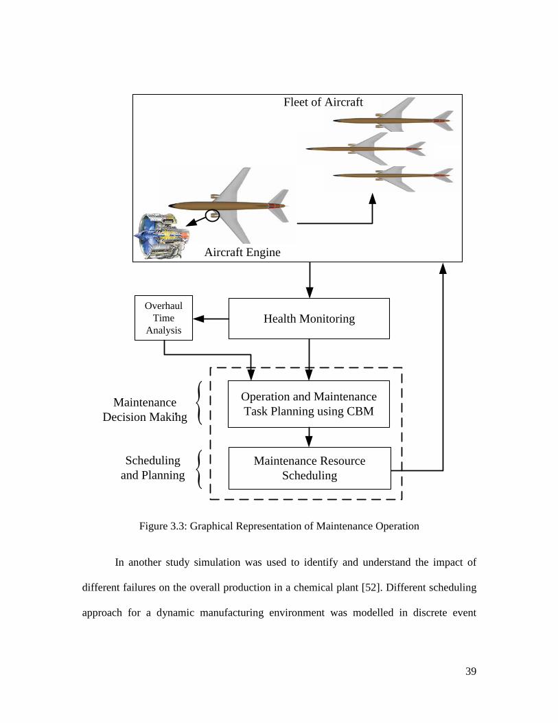
Health Monitoring
Operation and Maintenance Task Planning using CBM
Maintenance Resource Scheduling
Maintenance Decision Making
Scheduling and Planning
{{
Overhaul Time
Analysis
Aircraft Engine
Fleet of Aircraft
Figure 3.3: Graphical Representation of Maintenance Operation
In another study simulation was used to identify and understand the impact of
different failures on the overall production in a chemical plant [52]. Different scheduling
approach for a dynamic manufacturing environment was modelled in discrete event
39

simulation based on past performance [39]. Johanson et al. examined to what extend
discrete event simulation can be applied to evaluate the performance and the profit of a
manufacturing system. The results showed that there is a large potential to increase the
productivity when all scenarios are correctly modelled [40]. In line-production systems,
engineers did benefit from simulation application as they mimicked the system behaviour
to perform extended analysis to compare different scenarios and to support their decision-
making processes [78]. Van Den Bergh implemented DES in testing his methodology for
obtaining the optimal schedule for aircraft line maintenance personnel [37].
Bell studied two types of maintenance schedules in army aviation in term of
operational readiness. This study models the tradeoffs of one method versus the other
using discrete event simulation knowing the operational data set from a deployed aviation
unit. The effectiveness of each method is measured in the time each airframe is in for
mission [79].
A case study was conducted to compare traditional discrete event simulation
against an agent-based modeling approach that involved the implementation of two
functionally identical repair models based on a realistic aircraft gas turbine operation. It
was shown that agents were time-driven rather than event-driven. The discrete-event
model followed an event list which was faster and thus desirable [80].
An aviation industry investigated the use of three levels of aircraft maintenance.
This work examined the effect of maintenance resource sharing between facilities and a
centralized repair facility on a critical line replacement unit. Maintenance data was
collected and summarized into probability distributions and then was used in a discrete
40

event simulation model to examine the impact of changes to the maintenance structure.
Combining resources and personnel, independent versus sharing bases and cost
associated with shipping between them, effectiveness of processing time and machine
utilization were also considered [81]. In other works, modeling the life cycle cost of aero-
engine maintenance was studies [82].
From the forgoing, it is apparent that for the type of systems considered and the
kind of issues examined, DES is a useful tool that allows many operating conditions and
constraints to be included and modelled. To refresh, our goal is to develop aircraft engine
maintenance models using discrete event simulation that allow examination and
evaluation of various scenarios for a fleet of aircraft. As engines on an aircraft are
generally at different state of health, it is often one engine that initiates the need for
maintenance. To address the first objective of this thesis, many scenarios will be
examined. At the outset we state that models will be developed and analyses will be
performed to see while the aircraft is at the service facility, whether it is economical and
time-efficient to attend to other engines of that aircraft, and if so, determine the number
of engines that could be subjected to preventive maintenance.
3.4.1 Maintenance Model Development
A notable part of the work was to study health monitoring and engine inter-turbine
temperature sensor logs to extract useful data for simulations. The remainder of this
chapter shows how the structure of the models is developed; the simulations and their
results are reported in Chapter 4.
41
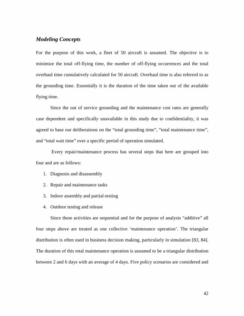
Modeling Concepts
For the purpose of this work, a fleet of 50 aircraft is assumed. The objective is to
minimize the total off-flying time, the number of off-flying occurrences and the total
overhaul time cumulatively calculated for 50 aircraft. Overhaul time is also referred to as
the grounding time. Essentially it is the duration of the time taken out of the available
flying time.
Since the out of service grounding and the maintenance cost rates are generally
case dependent and specifically unavailable in this study due to confidentiality, it was
agreed to base our deliberations on the “total grounding time”, “total maintenance time”,
and “total wait time” over a specific period of operation simulated.
Every repair/maintenance process has several steps that here are grouped into
four and are as follows:
1. Diagnosis and disassembly
2. Repair and maintenance tasks
3. Indoor assembly and partial-testing
4. Outdoor testing and release
Since these activities are sequential and for the purpose of analysis “additive” all
four steps above are treated as one collective ‘maintenance operation’. The triangular
distribution is often used in business decision making, particularly in simulation [83, 84].
The duration of this total maintenance operation is assumed to be a triangular distribution
between 2 and 6 days with an average of 4 days. Five policy scenarios are considered and
42
respective simulation models are developed using the Arena® Discrete Event Simulation
software.
The first four scenarios are preliminary defined such that when an aircraft is
scheduled for maintenance, the maintenance facility has the options of performing
maintenance on one, two, three or four engines. After these preliminary analyses are
conducted, in the next step all four scenarios are integrated into one main model. This
fifth model is so constructed to examine and to select one of the four maintenance
scenarios (one, two, three or four engines) for every arriving aircraft based on a number
of user-defined conditions. It is envisaged that with proper selection of these condition
effective policies can be developed. All these scenarios are described in detail in the
remainder of this chapter.
Scenarios Considered
Each of the 50 aircraft within the fleet is assumed to have four engines. Each of the 200
total engines is assigned a RTTF value randomly drawn between 7,000 and 10,000 hours,
based on and obtained from the typical logged data. Once all the aircraft are “created” (in
the paradigm of the simulation software), and entered into the model, a normal
“operating” status is assumed. Since Discrete Event Simulation (DES) is used, the “time”
is advanced in discrete steps to the time of the pending event (which then becomes the
“current time” or “Time Now”: TNOW in the language of the software) where the
statistics and status of every entity of the model become available. The statistics and
other data are continually and automatically updated during the simulation at every event
43
times by the software, and subsequently are used for decision making by the user as
needed.
A significant amount of time is consumed when an aircraft is taken away from its
normal flying service and sent for repair or maintenance. As briefly mentioned earlier,
this is usually triggered due to the status of ‘one’ engine. While an aircraft is at the
service/maintenance facility more than one engine can be serviced (upgraded/updated in
health status). This may appear to be more economical than attending to one engine only.
However, this very much depends on the service history of the engines. The combined
simulation model is developed such that more than one engine can be serviced depending
on certain user set thresholds. The threshold values are based on TOW or RTTF, and can
be altered to examine numerous alternatives to arrive at an optimal arrangement.
Since DES is not a self-optimizing method, with experimental planning, a
manageable number of cases are simulated to determine effective solutions. The
simulation model produces many statistics that must be carefully interpreted and used to
improve the maintenance operations in many aspects. However, it appears that the single
most important factor here is the ‘overall cumulative overhaul time’.
3.5 Building the Models
As shown in Figure 3.4, the overall maintenance procedure consists of five blocks.
System is initialized when an aircraft enters the maintenance model. A random value of
RTTF between 7000 to 10,000 hours (obtained from engine data-logs) is assigned to each
engine and then aircraft proceeds to flying operation. Grounding for maintenance is
44
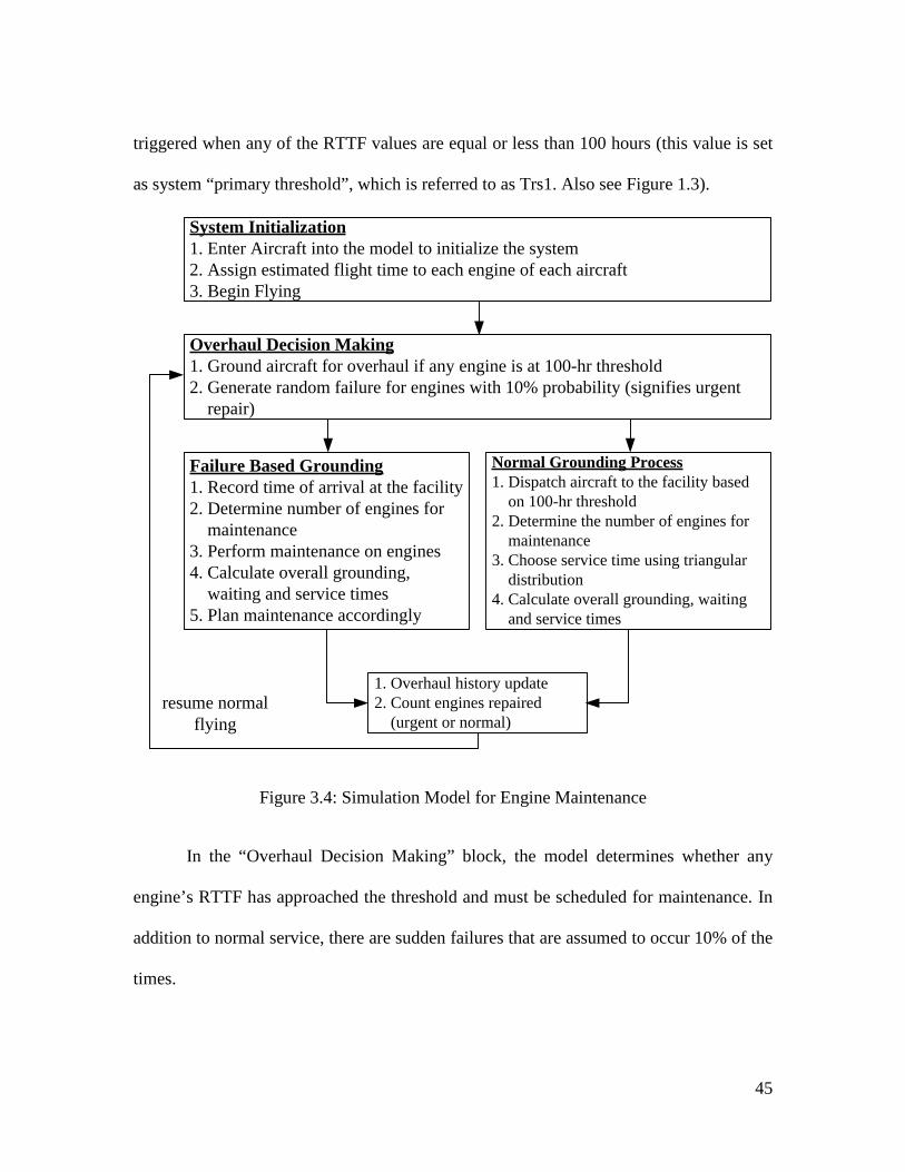
triggered when any of the RTTF values are equal or less than 100 hours (this value is set
as system “primary threshold”, which is referred to as Trs1. Also see Figure 1.3).
System Initialization1. Enter Aircraft into the model to initialize the system 2. Assign estimated flight time to each engine of each aircraft3. Begin Flying
Overhaul Decision Making1. Ground aircraft for overhaul if any engine is at 100-hr threshold2. Generate random failure for engines with 10% probability (signifies urgent repair)
Failure Based Grounding1. Record time of arrival at the facility2. Determine number of engines for maintenance3. Perform maintenance on engines4. Calculate overall grounding, waiting and service times5. Plan maintenance accordingly
1. Overhaul history update2. Count engines repaired (urgent or normal)
resume normal flying
Normal Grounding Process1. Dispatch aircraft to the facility based on 100-hr threshold2. Determine the number of engines for maintenance3. Choose service time using triangular distribution4. Calculate overall grounding, waiting and service times
Figure 3.4: Simulation Model for Engine Maintenance
In the “Overhaul Decision Making” block, the model determines whether any
engine’s RTTF has approached the threshold and must be scheduled for maintenance. In
addition to normal service, there are sudden failures that are assumed to occur 10% of the
times.
45

The service time is chosen using triangular distribution with a minimum of 2,
average of 4 and a maximum of 6 days. The wait, service and total grounding times are
determined and statistics are collected. Upon the completion of maintenance, the aircraft
returns to normal flying operation.
In the “Failure Based Grounding” block, once the system generates a sudden
random failure, the aircraft is placed in the queue to enter the service facility. From
engine RTTF values, the model determines whether any of the other engines should also
be serviced while the aircraft is at the facility for maintenance.
At the final stage of the service, before the aircraft resume its flying operation, the
overhaul history is updated and total number of engines serviced is recorded.
If the maintenance facility is to perform maintenance on more than one engine,
the estimated time from the triangular distribution is multiplied by 1.5, 2, and 2.5 for two,
three and four engine maintenance, respectively. The service times are not multiplied by
the respective number of engines, since much of the set-up and preparation times are not
repeated.
The simulation run time is set to 200,000 hours. In fact, it is common to run
simulations for prolonged periods but apply the results to a shorter time span. This large
duration assures that the events and measures within the model reach steady state
conditions. Further, the output data were averaged over multiple simulation runs. The
suitable number of replications was found to be 5 and any larger number did not notably
affect the convergence of the output data. This is demonstrated in chapter 4 when the
46

simulations are run. In the following sections each of the scenarios are explained and the
results are discussed.
3.5.1 1-Engine Maintenance
In this scenario, the maintenance model is set to perform service on one engine only. As
shown in Figure 3.5, after any of the four engines reaches the primary threshold (Trs1),
the aircraft is grounded, maintenance is performed, RTTF and the engine condition are
updated and the grounding, wait and service times are calculated.
When an aircraft is released back into the normal operation, the model continues
to monitor and evaluate the TOW information until the threshold is reached again by one
of the engines. The threshold is a user-defined variable and can be changed to arrive at
any other optimal or desirable maintenance policy depending on what is desired.
There are four conditions defined in the decision block. Every time the model
attempts to schedule a service, the current conditions of the four engines (RTTF1,
RTTF2, RTTF3, and RTTF4) are examined. For instance, let us use a condition where
first engine requires maintenance. If we set the threshold to 100 hours, and assume the
following arbitrary values: RTTF1 = 80, RTTF2 = 200, RTTF3 = 250 and RTTF4 = 350,
the condition is such that only RTTF1 is below 100. Although in this example for clarity
the lowest RTTF is given a value less than 100, and symbolically in scenarios 2, 3 and 4,
and the Figures 3.5 to 3.8 the ‘check condition’ is shown as ‘RTTF<100’, however, the
construct of the simulation models are such that the lowest RTTF is selected at exactly
47

100 hours. At the end of the service of the engine with the lowest RTTF, the maintenance
history, and the total number of engines serviced, either urgent or normal, are updated.
Time Record
DecideTime
Calculation
Engine Overhaul
Aircraft Arrival
resume normal operation resume normal operation
System Initialization
Overhaul History Update
RTTF Resetting
Aircraft Grounding ProcessSingle Engine
RTTF<100 Overhaul Process
FlyingRTTF
Urgent Service (Repair)
Figure 3.5: Block Diagram for 1-Engine Maintenance
3.5.2 2-Engine Maintenance
In the second scenario, the model carries out the maintenance on two of the engines of
the aircraft that arrives at the facility. For this case, Figure 3.6 represents the model
overview which is very similar to that of the 1-Engine maintenance.
In this scenario, after initializing the simulation, the model determines the engines
with the two lowest RTTF values. Once the first engine of the aircraft is selected for
maintenance using the primary threshold, the model checks the other three engines in
order to find the second lowest RTTF. The second engine is selected by comparing the
three remaining engines against the first one. For instance, assuming arbitrary values of
RTTF1 = 80, RTTF2 = 200, RTTF3 = 250 and RTTF4 = 350, the model selects engines 1
and 2 from checking the following conditions:
48

(RTTF1 < 100)
(RTTF1 < RTTF3) and (RTTF1 < RTTF4)
(RTTF2 < RTTF3) and (RTTF2 < RTTF4)
In case of an urgent service, the same procedure is followed. Once an aircraft is
destined to the facility for service, the status of the other engines is checked to identify
the second engine with the lowest RTTF.
Time Record
Decide
Engine Overhaul
Aircraft Arrival
resume normal operationresume normal operation
System Initialization
Overhaul History Update
Aircraft Grounding ProcessEngine #1: RTTF<100
Engine #2: 2nd lowest
2-Engine Maintenance
FlyingTime
CalculationRTTF
ResettingOverhaul Process
Urgent Service (Repair)
RTTF
Figure 3.6: Block Diagram for 2-Engine Maintenance
3.5.3 3-Engine Maintenance
For this scenario, as illustrated in Figure 3.7, the simulation model is designed to perform
maintenance on three engines once an aircraft arrives at the facility. Similar to the last
two scenarios, the need for maintenance is initiated based on the status of one engine that
has a flying time, RTTF1, less than the defined primary threshold (Trs1). To identify the
49
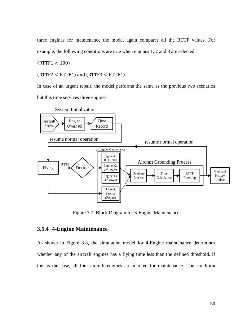
three engines for maintenance the model again compares all the RTTF values. For
example, the following conditions are true when engines 1, 2 and 3 are selected:
(RTTF1 < 100)
(RTTF2 < RTTF4) and (RTTF3 < RTTF4)
In case of an urgent repair, the model performs the same as the previous two scenarios
but this time services three engines.
Time Record
Decide
Engine Overhaul
Aircraft Arrival
resume normal operation resume normal operation
System Initialization
Overhaul History Update
Aircraft Grounding ProcessEngine #1: RTTF<100
Engine #2: 2nd lowest
3-Engine Maintenance
Engine #3: 3rd lowest
FlyingRTTF
Urgent Service (Repair)
Time Calculation
RTTF Resetting
Overhaul Process
Figure 3.7: Block Diagram for 3-Engine Maintenance
3.5.4 4-Engine Maintenance
As shown in Figure 3.8, the simulation model for 4-Engine maintenance determines
whether any of the aircraft engines has a flying time less than the defined threshold. If
this is the case, all four aircraft engines are marked for maintenance. The condition
50

defined in the “Decide” block is true only when any of RTTF1, RTTF2, RTTF3 or
RTTF4 is less than the threshold value as shown below:
(RTTF1 < 100) or (RTTF2 < 100) or
(RTTF3 < 100) or (RTTF4 < 100)
Time Record
Decide
Engine Overhaul
Aircraft Arrival
Resume normal operationResume normal operation
System Initialization
Overhaul History Update
Aircraft Grounding ProcessEngine #1: RTTF<100
Engine #2Engine #3Engine #4
4-Engine Maintenance
FlyingRTTF
Time Calculation
RTTF Resetting
Overhaul Process
Urgent Service (Repair)
Figure 3.8: Block Diagram for 4-Engine Maintenance
3.5.5 Integrated Scenario Selection (ISS) Engine Maintenance
The consideration of the previous four scenarios was to examine whether any “fixed”
policy, say 2-Engine maintenance, can be justified; where the user can set a threshold and
arrive at a good policy. However, using a “fixed” policy seems rather indiscriminate and
somewhat unsystematic. The purpose of the foregoing scenarios was to have the models
available for the management should they decide on experimenting with such fixed
policies. Whereas any of the policies appear an unlikely choice, the greatest and perhaps
51

the only advantage can be realized if the maintenance facility is “permanently” set up to
perform the service systematically and fast.
In this section, a detailed model is proposed, which is referred to as the Integrated
Scenario Selection (ISS). As opposed to the previous four scenarios, where the policy
was to consistently use only one fixed policy, this model combines all four previous
scenarios. In other words, this model examines all scenarios, before selecting optimal
number of engines for maintenance every time an aircraft is to pass through the service
facility.
The maintenance is initiated by the needs of one engine, which requires service
and enters the overhaul system, as illustrated in Figure 3.9. The “Decide” block identifies
the particular engine that has RTTF less than the primary assigned threshold (Trs1). In
this model a secondary threshold (Trs2) is introduced as a variable which can be altered
in repeated simulations in order to determine the condition for optimum maintenance.
Within the simulations Trs2 is used to determine the “relative difference” of RTTFs
between the engines. Once a difference is within the range, the respective engine is also
selected for overhaul. The value assign to this threshold can play a major role in selecting
the engines. In fact, Trs2 is a decision variable, and will be used and discussed in the next
chapter.
Let us illustrate the engine selection of this model by using an example. Assuming
hypothetical values of RTTF1 = 80, RTTF2 = 200, RTTF3 = 250, RTTF4 = 350, Trs1 =
100 and Trs2 = 110 hours, the following conditions lead to maintenance being carried out
on two Engines:
52

(RTTF1 < 100) and (RTTF2 − RTTF1 < 110) and
(RTTF3 − RTTF1 > 110) and (RTTF4 − RTTF1 > 110)
Each of the devised individual scenarios (1-Engine, 2-Engine, 3-Engine and 4-
Engine), and the Integrated Scenario Selection (ISS) engine maintenance have been
explained and their related modeling structures discussed. In the next chapter these
scenarios are built as models in Arena® discrete event simulation software. In addition,
statistics for each scenario is collected and discussed to decide on optimal aircraft
maintenance policy and planning.
53

Time Record
Decide
Engine Overhaul
Aircraft Arrival
resume normal operationresume normal operation
System Initialization
Aircraft grounding processSingle Engine
RTTF<100
Aircraft grounding processEngine #1: RTTF<100
Engine #2: 2nd lowest
2-Engine Maintenance
Overhaul History Update
Aircraft grounding process
Engine #1: RTTF<100
Engine #2: 2nd lowest
3-Engine Maintenance
Engine #3: 3rd lowest
Aircraft grounding processEngine #1: RTTF<100
Engine #2Engine #3Engine #4
4-Engine Maintenance
Flying
Urgent Service (Repair)
Urgent Service (Repair)
Urgent Service (Repair)
Urgent Service (Repair)
RTTF
Time Calculation
RTTF Resetting
Overhaul Process
Time Calculation
RTTF Resetting
Overhaul Process
Time Calculation
RTTF Resetting
Overhaul Process
Time Calculation
RTTF Resetting
Overhaul Process
Figure 3.9: Block Diagram for ISS Engine Maintenance
54

Chapter 4: Engines Maintenance Planning and Discrete Event Simulation Analysis
4 Engines Maintenance Planning and Discrete
Event Simulation Analysis
4.1 Introduction
Suggestions have been made to ensure that not only all the engines are maintained in an
efficient manner, but that their scheduled maintenance cycles are carried out
simultaneously so that the aircraft has fewer trips to the maintenance facility [85].
However, such pre-planned maintenance can be impractical and uneconomical. (In fact in
chapter 3, the 4-Engine maintenance is a related scenario.) After a short period of time in
operations, even for a new aircraft, the engines on the aircraft can and will begin to
behave and prove their ‘individuality’. Despite identical looks, due to statistical
55

variations in material properties, manufacturing and assembly, no two products are made
the same. With typically over 20,000 components, aircraft engines are no exception. Each
engine will deteriorate at its own pace and will require maintenance and service at its
own specific time. Subjecting all engines to the same maintenance schedule can thus be
uneconomical. Therefore, cost reduction may be achieved through other means such as
reducing downtime, repair costs and improving the quality of products and faster
services. Use of dynamic maintenance planning in a fleet, in other words condition-based
maintenance (CBM) rather than time-based maintenance will significantly contribute to
achieving this objective.
The purpose of this thesis is to conduct the analysis required to determine if CBM
is advantageous in comparison to the current periodic maintenance. This chapter presents
results obtained through implementation of CBM using discrete event simulation
software Arena® in order to arrive at an aircraft maintenance policy which minimizes the
total downtime and overall cost of the maintenance operations. Section 4.2 gives an
overview of the proposed engine maintenance scenarios and section 4.3 discusses the
simulation results. In section 4.4, the proposed method is validated through a secondary
discrete event simulation “Simio”.
4.2 Overview of Engine Maintenance Scenarios
To perform maintenance on aircraft, either due to a problem in one engine, or due to a set
time for service, a number of options are available. One option is to consider a policy in
which a ‘fixed’ number of engines are serviced. That is, the enterprise uses a policy in
56
which for any aircraft at the time of maintenance, consistently ‘𝑛’ engines are serviced.
For a four-engine aircraft, for instance, this will be 1-Engine, 2-Engine, 3-Engine or 4-
Engine choices. This may have the convenience that the maintenance facility is always
set-up to run a fixed routine. One can anticipate that this approach will most likely be
uneconomical. These options were examined in chapter 3. Another approach, which
seems plausible, is to service a ‘variable’ number of engines, based on engine status and
some reasonable set of conditions. In this section, we examine these options and policy
scenarios. For each of the scenarios outlined in chapter 3, in this chapter a model in
Arena® is developed and simulations carried out.
4.2.1 Maintenance Scenarios with a Fixed Number of Engines
As shown in Figure 4.1, the model starts by generating aircraft entities. The number of
aircraft is selected based on the user need. The next step is to assign specific attributes
which are characteristics or factors specific to an aircraft. ‘Entity’ and ‘Attribute’ are
technical terms used in most simulation software, as described for Arena® in chapter 3,
which refer to objects and their tagged-on data, respectively. One example of an attribute
is the aircraft ID that enables the modeller to track any aircraft in the model at any instant
of time. Another important attribute is RTTF values for each engine and this is
determined and assigned using a uniform distribution with a minimum of 7,000 and a
maximum of 10,000 hours. The variation takes into consideration the age of the aircraft
and the confidence in the degree of restoring the functionality of the engines after each
maintenance operation.
57

The current condition of each aircraft, i.e. RTTF, in the model must be known for
estimating the time of maintenance. Once the aircraft are put into operational flying
mode, the model checks the RTTF of all engines of each aircraft at the simulation “event
times”. For maintenance scenarios with more than 1-Engine, the engines with second and
third lowest RTTF, respectively, are selected. Referring to Figure 4.1, depending on the
policy being examined only one scenario from the block marked “Individual Scenario
Selection” is used for the entire simulation.
Re-assign RTTF Values for Repaired Engines
Create Aircraft
Resume Flying
Check for Condition1) Urgent Maintenance2) Normal Maintenance
(Find RTTF < 100 hrs)
Individual Scenario Selection1) 1-Engine 3) 3-Engine2) 2-Engine 4) 4-Engine
Maintenance Operation
(1, 2, 3, 4 Engine Maintenance)
grounding
Assign RTTF Uniformly Between (7000, 10000) hrs
Assign Specific
Attributes
queue
Figure 4.1: Maintenance Operation for “Fixed” Number of Engines
In addition, the model randomly generates sudden failure at the rate of 10% of all
maintenance events. The grounded aircraft joins a queue before it enters the maintenance
facility. At the completion of the service, the RTTF values are re-set before resuming
normal flying operation. At the conclusion of the simulation, the statistics generated
output are analyzed to make decisions that would improve the maintenance operations.
58

4.2.2 Integrated Scenario Selection (ISS) Maintenance
In ISS, as shown in Figure 4.2, the maintenance operation is very similar to the scenarios
for maintenance on a fixed number of engines. The difference in ISS is that the model
determines the number of engines for every maintenance instance based on the assigned
value for the secondary threshold (Trs2). The significance of this will be explained later.
Measure RTTF Values against Trs2
Engine Selection
Create Aircraft
Resume Flying
Check for Condition1) Urgent Maintenance2) Normal Maintenance
(Find RTTF < 100 hrs)
1) 1-Engine2) 2-Engine3) 3-Engine4) 4-Engine
Maintenance Operation
(ISS)
Scenario Selection
grounding
Assign RTTF Uniformly Between (7000, 10000) hrs
Assign Specific
Attributes
Re-assign RTTF Values for Repaired Engines
queue
Figure 4.2: Graphical Representation of Maintenance Operation for ISS
To initiate the simulation, and before aircraft resume flying, attributes are
assigned to each aircraft and values for RTTF are chosen uniformly between 7,000 and
10,000 hours based on the sample Inter-Turbine condition data. While flying, the model
checks the conditions of the aircraft engines. Once the minimum RTTF value is reached
or a failure occurs (set at 10% of all maintenance events) the aircraft is destined for
grounding. Before entering the maintenance facility, the differences between the RTTF
values for the other engines are compared against the Trs2 to select an appropriate
maintenance scenario (number of engines for maintenance). At the end of the
maintenance operations, statistics are collected for analysis and decision making.
59

4.3 Arena® Simulations
Simulation for individual “fixed” number of engines and ISS maintenance models for a
fleet of 50 aircraft are run for 200,000 hours of fleet operation. In order to populate the
simulation model with the 50 aircraft, they enter the model at an accelerated arrival with
an inter-arrival time of 0 to 200 hours distributed uniformly over the range. At this rate
(an average of 100 hours), within approximately the first 5000 hours of simulation run all
50 aircraft will have entered and dispersed throughout the model. With a random
assignment of RTTF, it is safe to assume that the fleet will soon be in near normal
operation status. In other words, the model transient will no longer be present.
4.3.1 Individual Maintenance Scenarios
In this section, first we study the results of the simulation for individual maintenance
scenarios where a “fixed” number of engines per aircraft are serviced at the maintenance
facilities. This starts by discussing the overall simulation stability and its appropriate
replication number selection, and then a conclusion is made for optimal maintenance
planning on the basis of overall cumulative time values. Using 1-Engine maintenance as
an example, Figure 4.3 and 4.4 are the representation of Figure 4.1 modelled in Arena®.
60

Figure 4.3: Screenshot of the Entire Arena® 1-Engine System
(a)
(b)
Figure 4.4: Screenshot of blocks: (a) Engine Selection for Maintenance, and (b) Service of Engines
See Figure 4.6
See Figure 4.6
61

Simulation Stability
One of the useful estimations required before running the simulation is the suitable
number of replications which ensures the convergence of the output data to steady state
averages and levels. For implementing this, average value of one of the outputs,
specifically “Average Waiting Time”, which represents the average time each aircraft
spends in maintenance facility queue, was chosen. As illustrated in Figure 4.5, The
Average Waiting Time for all scenarios appear steady with respect to the number of
replications, but any number of replications greater than four seems reasonable as the
average waiting time of each individual scenario converge to a more steady level, and
that it will ensure the stability of other outputs. The number of replications is set at 5 for
the simulations conducted.
Figure 4.5: Estimating Replication Number for Individual Scenarios
Another criterion to consider after deciding the number of replication is the
stability and uniformity of the simulation output for all the aircraft in the fleet. As shown
0
100
200
300
400
500
1 2 3 4 5 6 7 8 9 10
Aver
age
Wai
ting
Tim
e (h
rs)
Replication Number
1-Engine 2-Engine 3-Engine 4-Engine
62
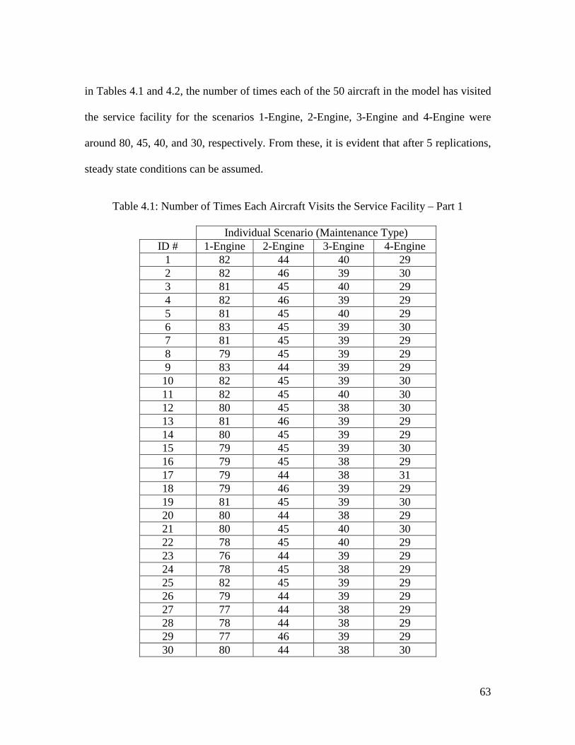
in Tables 4.1 and 4.2, the number of times each of the 50 aircraft in the model has visited
the service facility for the scenarios 1-Engine, 2-Engine, 3-Engine and 4-Engine were
around 80, 45, 40, and 30, respectively. From these, it is evident that after 5 replications,
steady state conditions can be assumed.
Table 4.1: Number of Times Each Aircraft Visits the Service Facility – Part 1
Individual Scenario (Maintenance Type) ID # 1-Engine 2-Engine 3-Engine 4-Engine
1 82 44 40 29 2 82 46 39 30 3 81 45 40 29 4 82 46 39 29 5 81 45 40 29 6 83 45 39 30 7 81 45 39 29 8 79 45 39 29 9 83 44 39 29 10 82 45 39 30 11 82 45 40 30 12 80 45 38 30 13 81 46 39 29 14 80 45 39 29 15 79 45 39 30 16 79 45 38 29 17 79 44 38 31 18 79 46 39 29 19 81 45 39 30 20 80 44 38 29 21 80 45 40 30 22 78 45 40 29 23 76 44 39 29 24 78 45 38 29 25 82 45 39 29 26 79 44 39 29 27 77 44 38 29 28 78 44 38 29 29 77 46 39 29 30 80 44 38 30
63

Table 4.2: Number of Times Each Aircraft Visits the Service Facility – Part 2
Number of Visits to Service Facility ID # 1-Engine 2-Engine 3-Engine 4-Engine 31 81 43 39 28 32 77 43 38 29 33 82 45 38 29 34 78 44 38 28 35 83 46 38 30 36 79 43 37 28 37 77 44 37 29 38 77 44 38 29 39 79 44 38 29 40 77 44 38 29 41 77 45 37 28 42 79 43 38 29 43 79 44 38 30 44 81 46 38 29 45 77 45 38 29 46 77 43 38 29 47 78 44 39 29 48 79 43 38 28 49 81 43 38 28 50 77 42 37 29
Statistical Results
After reaching steady state by establishing appropriate replication runs, the next
step is collecting conclusive simulation results for maintenance planning. Table 4.3
presents the preliminary comparison between cumulative service times, and the total
number of aircraft and corresponding number of engines serviced for the given scenarios
for 200,000 hours of fleet operation.
64

Table 4.3: Preliminary Simulation Results for Individual Maintenance Scenarios
Maintenance Type
Total Service Time
(Hours)
Number of Aircraft Serviced (Normal)
Number of Aircraft Serviced (Urgent)
Total Aircraft Serviced
Service Time Per Aircraft (Hours)
Single Engine
Serviced (Hours)
1-Engine 389,626 3,661 400 4,061 95.94 95.94
2-Engine 327,820 2,052 231 2,283 143.59 95.72
3-Engine 371,921 1,740 198 1,938 191.91 95.95
4-Engine 356,550 1,332 154 1,486 239.94 95.98
Facilities can be permanently set up to efficiently perform maintenance on a fixed
pre-determined number of engines, i.e. 1-Engine, 2-Engine, 3-Engine or 4-Engine,
depending on the resource availability and the facility capacity. See also the discussion in
section 3.5.5. For instance, to perform and complete 4-Engine maintenance in an optimal
time, a facility needs to schedule more staff overtime, and to assess the inventory and
spare part availability. These resource decision factors have weights and costs in $/hour
associated with their importance that can play a major part in making the final decisions.
However, these cost data are not available in this study and all the discussions are solely
on time-based parameters such as engine RTTF.
In each of the four scenarios, maintenance was triggered when one engine’s
RTTF was at the threshold (Trs1) level and it required service.
A facility with a capacity to perform maintenance on a maximum of two engines
at a time, can handle 1-Engine and 2-Engine maintenance. This analysis (1-Engine vs. 2-
Engine) determines which type is the most optimal planning considering the lowest
grounding time and highest flying hours. For the same reason, a facility with a capacity
65

and resources available for three-engine maintenance, can consider 1-Engine through 3-
Engine maintenance.
The data presented in Table 4.3 is informative. However, one of the drawbacks of
these individual scenarios, specifically the analysis of the results, is that they are not
intuitive and conclusive since a multitude of factors must be concurrently assessed. These
factors will require a weight associated with their importance. Once these influential
factors such as cost of personnel, assembly, part replacement, and facility usage (these
are unknown due to confidentiality) are taken into consideration, these differences
become more pronounced for decision making.
From preliminary individual scenario results it became evident that there is no
practical way of distinguishing and selecting the best scenario when considering all four
scenarios for a facility with a capacity of 4-Engine maintenance. Although amongst the
four scenarios one scenario may prevail, the implementation of a single fixed scenario
will unlikely be optimal or near optimal. As such, more detailed analysis of the individual
scenarios is required in order to draw better conclusion in terms of which scenario truly
prevails or offer some relative merits.
As to evaluation of individual scenarios in detail, various results extracted from
the simulation output are used to compare them as shown in Table 4.4. Some examples of
the data obtained for 200,000 hours of simulations are as follows: “Total Grounding
Time”, “Total Flying Time”, “Total Service Time”, and “Total Waiting Time”. In
addition, the average time values are also obtained from the simulations as shown in
Table 4.5. The plots of these average values versus times are provided in Appendix A.
66

Table 4.4 shows that both 1-Engine and 3-Engine policies have the highest total
waiting and service times and consequently, they have the highest total grounding times.
The results show that the most favourable scenarios, based on the number of hours, are 2-
Engine and 4-Engine maintenance due to their lower total grounding times and higher
total flying times.
Table 4.4: Simulation Results for Individual Maintenance Scenarios – Part 1
Maintenance Type
Average Queue Length
(Number Waiting)
Total Waiting
Time (Hours)
Total Service Time
(Hours)
Total Grounding
Time (Hours)
Total Flying Time
(Hours)
1-Engine 8.68 1,768,092 389,626 2,159,734 7,828,381
2-Engine 1.33 270,037 327,820 598,684 9,339,882
3-Engine 2.91 591,295 371,921 964,091 8,970,816
4-Engine 1.24 252,223 356,550 609,331 9,282,785
When the maintenance follows 1-Engine policy, the chances of any other engine
approaching the 100 hours primary threshold is much higher than with the other
scenarios. As a result, soon after resuming normal flying, the aircraft is grounded again
for service of another single engine, thus the system accumulates the highest total
grounding time. In addition, there are more aircraft waiting for service which reflects in
the longer queue length. This is a recurring event throughout the 1-Engine maintenance
policy.
67

Table 4.5: Average Time Values for Individual Maintenance Scenarios – Part 2
Maintenance Type
Average Waiting Time
(Hours)
Average Service Time
(Hours)
Average Grounding Time
(Hours)
Average Flying Time
(Hours)
1-Engine 439.34 96.51 535.34 1,927.42
2-Engine 118.41 144.13 262.53 4,095.29
3-Engine 306.33 192.16 498.49 4,635.21
4-Engine 171.08 240.30 411.30 6,245.16
The 3-Engine maintenance policy results in a similar behaviour as the 1-Engine
maintenance. Upon reaching the primary threshold of 100 hours by any of the aircraft
engines, 3-Engine maintenance is performed and the aircraft resumes its normal flying.
However, it is very likely that the remaining fourth engine’s RTTF reaches the 100 hours
soon after and, therefore; the aircraft needs to be grounded again for maintenance. This in
fact ranks the 3-Engine scenario second in terms of having the highest total waiting and
grounding times and a long average queue length of 3 aircrafts considering a fleet of 50
aircraft.
In 2-Engine scenario, maintenance favourably alternates between pairs of engines.
The simulation shows that with 2-Engine maintenance scenario, the lowest total
grounding and waiting times is achieved. It is evident that when engines are serviced in
pairs, they can fly for longer hours and achieve higher flying times. Consequently,
average queue length is low and the waiting and grounding times are relatively lower
compared to that of the 1-Engine and 3-Engine scenarios.
68
In regards to 4-Engine maintenance, it is shown that it has the second highest total
flying time. This is due to the fact that, regardless of the values of engine RTTF,
maintenance is performed on four engines. This to some extent prolongs the flying hours
with an average flying time of 6,200 hours after every maintenance operation, unless the
aircraft requires an urgent repair. Since the aircrafts are mostly in flying operation, the
system barely sees a line-up and thus, it achieves the lowest total waiting time in the
system. It was discussed earlier that cost-wise, this may not be a good policy.
In order to determine whether 2-Engine prevails over the 4-Engine policy or vice
versa, a multitude of factors (such as the costs of downtime, technicians, spare-part, etc.)
must be concurrently assessed for each scenario. However, what this study can suggest is
optimal planning on the basis of cumulative operation and maintenance hours. It is,
however, up to the industrial user to fully assess the outcome of the maintenance
operation based on resource availability and their existing operational costs and the
weights associated with their importance.
4.3.2 Integrated Scenario Selection (ISS)
In this section, simulation results of the ISS maintenance policy for a fleet of 50 aircraft
over 200,000 hours of operation are presented and discussed. Aircraft are modelled to
enter the system at an accelerated rate using a uniform distribution with inter-arrival time
of between 0 to 200 hours distributed uniformly over the range. At this rate (an average
of 100 hours), within approximately the first 5000 hours of simulation run all 50 aircraft
69
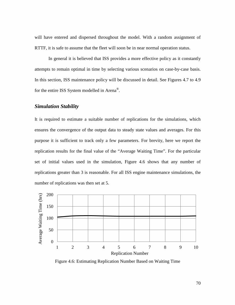
will have entered and dispersed throughout the model. With a random assignment of
RTTF, it is safe to assume that the fleet will soon be in near normal operation status.
In general it is believed that ISS provides a more effective policy as it constantly
attempts to remain optimal in time by selecting various scenarios on case-by-case basis.
In this section, ISS maintenance policy will be discussed in detail. See Figures 4.7 to 4.9
for the entire ISS System modelled in Arena®.
Simulation Stability
It is required to estimate a suitable number of replications for the simulations, which
ensures the convergence of the output data to steady state values and averages. For this
purpose it is sufficient to track only a few parameters. For brevity, here we report the
replication results for the final value of the “Average Waiting Time”. For the particular
set of initial values used in the simulation, Figure 4.6 shows that any number of
replications greater than 3 is reasonable. For all ISS engine maintenance simulations, the
number of replications was then set at 5.
Figure 4.6: Estimating Replication Number Based on Waiting Time
0
50
100
150
200
1 2 3 4 5 6 7 8 9 10
Aver
age
Wai
ting
Tim
e (h
rs)
Replication Number
70

Figure 4.7: Screenshot of the Entire Arena® ISS Model
See Figure 4.8
See Figure 4.9
71

Figure 4.8: Screenshot of the Maintenance Decision Block
Figure 4.9: Screenshot of the Statistical Data Collection Block
Maintenance Decision Block
72
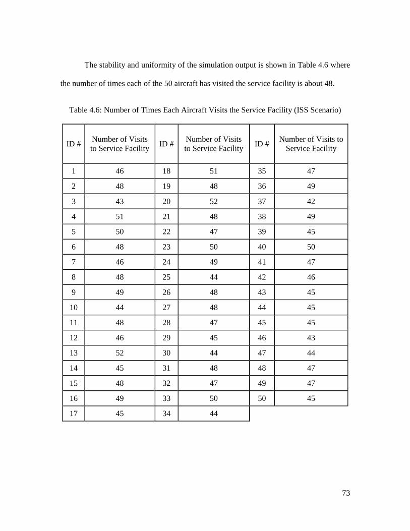
The stability and uniformity of the simulation output is shown in Table 4.6 where
the number of times each of the 50 aircraft has visited the service facility is about 48.
Table 4.6: Number of Times Each Aircraft Visits the Service Facility (ISS Scenario)
ID # Number of Visits to Service Facility ID # Number of Visits
to Service Facility ID # Number of Visits to Service Facility
1 46 18 51 35 47
2 48 19 48 36 49
3 43 20 52 37 42
4 51 21 48 38 49
5 50 22 47 39 45
6 48 23 50 40 50
7 46 24 49 41 47
8 48 25 44 42 46
9 49 26 48 43 45
10 44 27 48 44 45
11 48 28 47 45 45
12 46 29 45 46 43
13 52 30 44 47 44
14 45 31 48 48 47
15 48 32 47 49 47
16 49 33 50 50 45
17 45 34 44
73

Statistical Results
Table 4.7 shows the breakdown of the different types of services performed for
selected aircraft ID. One of the advantages of the proposed method is that it tracks every
entity (aircraft) individually within the model and collects relevant information regarding
its service and maintenance, as well as the fleet as a whole.
Table 4.7: Number of Different Service Type for Sample Selected Aircraft
Aircraft ID #
Total 1-Engine
Type Service
Total 2-Engine
Type Service
Total 3-Engine
Type Service
Total 4-Engine
Type Service
Total Aircraft Serviced
Total Sudden Failure Service
1 15 15 15 13 50 4
2 14 14 14 15 44 2
3 16 16 15 13 55 7
4 15 15 13 15 53 6
5 15 14 14 15 50 3
15 14 14 17 14 54 8
20 13 14 14 13 44 0
30 14 13 15 13 47 4
40 13 15 14 13 48 4
50 14 14 15 14 48 4
Many different results can be obtained from simulating the model. Table 4.8
shows the counts of different services performed during the simulations for the entire
fleet. The mandatory primary threshold was set as 𝑇𝑟𝑠1 = 100 hours, and the secondary
threshold, Trs2, was used as the policy optimization variable for the 21 cases assessed.
74

Table 4.8: ISS Engine Maintenance Policy Simulation Results – Part 1
Case #
Trs2 (hrs)
1-Engine Service Count
2-Engine Service Count
3-Engine Service Count
4-Engine Service Count
1 100 3,776 165 2 0
2 200 3,513 296 11 0
3 300 3,338 397 19 0
4 400 3,104 536 13 0
6 600 2,710 716 43 1
7 800 2,290 878 90 2
8 1,000 1,886 1,030 132 1
9 1,200 1,532 1,167 174 4
10 1,300 1,409 1,245 175 10
11 1,400 1,279 1,254 219 8
12 1,500 1,071 1,355 231 11
13 1,600 926 1,434 229 16
14 1,700 719 1,570 203 18
15 1,800 643 1,602 224 16
16 1,900 536 1,638 237 19
17 2,000 562 1,491 321 25
18 2,100 467 1,531 327 35
19 2,200 465 1,422 406 41
20 2,300 489 1,355 449 41
21 2,400 439 1,296 490 60
With simulation run time of 200,000 hours and a fleet of 50 aircrafts, there will be
a cumulative available ‘time’ of 10 × 106 hours. This is roughly equal to the sum of
75

‘total flying time’ and ‘total grounding time’. Therefore, these measures are
complementary and either can be used as one of the most important decision factors.
To further evaluate ISS in detail, various data are extracted from the simulation
outputs as shown in Tables 4.8 and 4.9. The average values of some other parameters
have also been extracted and plotted versus time, and these are given in Appendix B.
Referring to the data presented in Tables 4.8 and 4.9 (and in fact elsewhere too),
as alluded earlier, we focus our discussions on pure time-based facts and figures.
However, the industrial user must apply weights and proprietary cost data associated with
the time-based factors in their decision making processes.
As concluded from individual scenarios, the optimal maintenance occurs with the
2-Engine type. In the ISS maintenance, too, this important finding emerges around case
#16 (Table 4.8), where the greatest number of services is of 2-Engne type at the
secondary threshold (Trs2) of 1,900 hours.
The column showing the total grounding time in Table 4.9 is in fact the total of
waiting and service times. For ‘any cost rate’, it is envisaged that the minimum cost will
emerged around case #15, corresponding to the secondary threshold (Trs2) of 1,900
hours. The total cumulative operation hours of simulation (total flying and grounding
hours) for each case are seen to be near the expected 10 × 106 hours. It is also seen from
Table 4.8 that 2-Engine service has been dominant as expected, recalling the inferences
made during the discussion of the individual scenarios.
The total waiting time and the average queue length, from Table 4.9, are the
indication of the ‘capacity’ of service facility. The user may interpret this “queue time”
76

based on their priorities and finances, and run new simulation cases by proposing
increased capacity, for example (Chapter 5, provides convenient means for this types of
assessment).
Table 4.9: ISS Engine Maintenance Policy Simulation Results – Part 2
Case # Trs2 (hrs)
Average Queue Length
Total Waiting
Time (hrs)
Total Service
Time (hrs)
Total Grounding Time (hrs)
Total Flying
Time (hrs)
1 100 5.41 1,103,628 387,109 1,492,605 8,506,604
2 200 5.11 1,039,436 381,042 1,422,308 8,542,303
3 300 4.38 889,829 378,962 1,270,559 8,683,512
4 400 4.11 836,802 374,773 1,213,272 8,771,029
5 500 3.68 749,198 374,065 1,124,872 8,851,988
6 600 3.30 670,826 371,859 1,044,193 8,930,979
7 700 3.59 728,767 365,207 1,095,506 8,861,213
8 800 3.07 625,504 361,797 988,764 8,999,748
9 900 2.59 526,602 361,966 889,947 9,092,763
10 1,000 2.73 553,492 353,942 908,719 9,053,389
11 1,500 1.81 368,337 343,892 713,312 9,255,306
12 1,600 1.61 328,105 340,807 669,931 9,297,291
13 1,700 1.71 348,352 337,805 687,124 9,271,759
14 1,800 1.49 302,638 336,587 640,153 9,322,439
15 1,900 1.30 263,487 335,906 600,282 9,350,188
16 2,000 1.53 309,866 334,084 644,838 9,302,049
17 2,100 1.45 293,287 335,838 630,020 9,330,727
18 2,200 1.37 278,412 334,008 613,334 9,349,198
77

Clearly, increased capacity reduces the grounding time (equally the queue length
and service time) and thus, there will be fewer number of aircraft in the queue. This will
lead to a new state-of-affairs and total cost status; whereby the user can make an
economic analysis of the capital invested in increasing the capacity of the service facility,
and the return on investment in reducing grounding time.
The average values for notable cases of 10 through 18 representing Trs2 values of
1,000 to 2,200 hours (Table 4.9) are also given in Table 4.10.
Table 4.10: Simulation Average Time Values for ISS
Case # Trs2 (hrs)
Average Wait Time
(hrs)
Average Service
Time (hrs)
Average Grounding Time (hrs)
Average Flying
Time (hrs)
10 1,000 182 116.59 298.53 2,969.32
11 1,100 155.99 118.15 274.18 3,045.76
12 1,200 179.38 121.41 300.92 3,160.9
13 1,300 140.8 123.15 263.98 3,252.77
14 1,400 150.53 126.38 277.01 3,339.88
15 1,500 138.5 129.4 267.86 3,469.03
16 1,600 126.34 131.33 257.67 3,569.04
17 1,700 139.07 135.08 274.26 3,693.95
18 1,800 122.12 135.95 258.1 3,751.51
19 1,900 108.84 138.74 247.53 3,847.83
20 2,000 129.52 139.76 269.31 3,877.49
21 2,100 124.82 142.79 267.45 3,953.72
22 2,200 119.67 143.6 263.27 4,005.68
78

4.4 Model Verification for Individual Engine Maintenance
Scenarios Using Simio Discrete Event Simulation
As stated earlier, one of the challenges associated with this study was the confidentiality
issue and therefore, unavailability of real data related to the fleet operation, failures,
repairs and maintenance. However, as a standard practice, simulation models must be
verified, and the results validated if possible. Due to inaccessible data, the verification,
and to some extent validation through extended verification, are performed through a
secondary separate simulation modeling. As a result, “Simio” as an alternative simulation
tool was chosen to model and replicate the existing individual scenarios (1-Engine, 2-
Engine, 3-Engine and 4-Engine maintenance).
Due to general similarity of simulation languages, only introductory comments are
provided and detailed modeling constructs and concepts of Simio are not reproduced.
4.4.1 Simio Discrete Event Simulation
Simio, similar to Arena®, is a simulation modeling framework that is designed to support
the object modeling paradigm. Although its framework is focused on object-oriented
modeling, it also supports a seamless use of multiple modeling paradigms including
event, process, object-based modeling. An object might be a machine, robot, airplane,
customer, ship, or any other entity that one might encounter in modeling a system. A
Simio model looks similar to the real system. It is built by combining objects that
represent the physical components of the system. The process of building an object is
79

very simple and completely graphical. There is no need to write programming code to
create new objects [86, 87].
Simio is a newly introduced discrete event simulation software that has been
applied to various cases in industry and healthcare systems [88-91]. Each step in Simio
model is a simple process such as holding the token for a time delay, seizing/releasing of
a resource, waiting for an event to occur, assigning a new value to a state, or deciding
between alternate flow paths.
4.4.2 Building the Models in Simio
Four separate models are built for simulation of 1-Engine, 2-Engine, 3-Engine and 4-
Engine maintenance scenarios. A graphical representation of one of these models is given
in Figure 4.10.
To initialize the system, 50 aircraft are created, and a Remaining Time to Fly
(RTTF) randomly drawn between 7,000 and 10,000 hours is assigned to each engine of
each aircraft. Same as before, grounding has two forms: 1) Normal Grounding Process
where the aircraft is sent for service when any engine’s RTTF value reaches the primary
threshold (Trs1) of 100 hours. 2) Emergency Grounding Process occurs when an urgent
maintenance is required. This failure is assumed to take place 10% of the times.
Referring to the overall maintenance block diagram (Figure 4.11), the
maintenance is initiated when aircraft enter the system. In addition to the RTTF values a
distinct ID number is also assigned to each aircraft. The ID numbers enable the
user/modeller to track any aircraft in the model at any time. The aircraft grounding occurs
80

when the primary threshold (Tr1=100 hours) is reached by any aircraft’s engines. When
an aircraft is grounded (either normal or urgent), the maintenance is performed on a pre-
set number of engines as defined in scenarios 1-Engine, 2-Engine, 3-Engine and 4-
Engine, respectively.
Figure 4.10: Graphical Representation of a Simio Model
As used in Arena® models, the maintenance processing times are drawn from a
triangular distribution with a minimum of 2, a maximum of 6 and an average of 4 days.
81

System Initialization1. Enter Aircrafts into the model to initialize the system2. Assign RTTF and attributes to each aircraft3. Begin flying
Overhaul Decision Making1. Ground aircraft for overhaul if any engine is at 100-hr threshold2. Generate random failure for engines with 10% probability (signifies urgent repair)
Failure Based Grounding1. Record time of arrival at the facility2. Determine number of engines for maintenance3. Perform maintenance on engines 4. Calculate overall grounding, waiting and service times5. Plan maintenance accordingly
1. Update overhaul history2. Re-set RTTF for engines repaired (normal and urgent)Resume Normal
Operation
Condition Based Grounding1. Dispatch aircraft to the facility based on 100-hr threshold2. Determine the number of engines for maintenance3. Choose service time using triangular distribution4. Calculate overall grounding, waiting and service times
Figure 4.11: Overall Maintenance Procedure Flow Diagram
The processing time is multiplied by 1.5, 2, and 2.5 for two, three, and four
engine maintenance, respectively. The First-in-First-Out discipline is used for the
maintenance facility queue. At the end of the overhaul and before resuming normal
flying, the maintenance history such as: grounding, waiting and service times are updated
and the required statistics collected.
82

4.4.3 Simulation Stability
It is required to estimate a suitable number of replications for the simulations. Following
the same process as in the Arena® simulations, and referring to Figure 4.12, choosing any
replication number greater than four seems reasonable as the average waiting time of
each individual scenario converges to a steady level. In simulations that follow, a
replication number of 5 is used.
Figure 4.12: Estimating Replication Number for Individual Scenarios for Simio
4.4.4 Verification
To verify the Arena® models and simulations, the maintenance scenarios with “fixed”
number of engines are modeled and simulated in “Simio” software. The outputs from
these simulations are compared with those generated by Arena® as shown in Tables 4.11 to
4.16. For each aircraft in each scenario, the following statistical data are collected:
0 50
100 150 200 250 300 350 400 450 500
0 5 10 15 20
Aver
age
Wai
ting
Tim
e (h
rs)
Replication Number
1-Engine 2-Engine 3-Engine 4-Engine
83

1. Total and average flying time
2. Total and average grounding time
3. Total and average waiting time
4. Total and average service time
5. Average queue length
Table 4.11: Average Values from Simio Simulations
Maintenance Type
Average Queue Length
(Number Waiting)
Average Wait Time
(Hours)
Average Service Time
(Hours)
Average Grounding
Time (Hours)
Average Flying Time
(Hours)
1-Engine 8.56 426.86 96.1 522.83 1,921
2-Engine 1.44 133.05 143.9 276.64 3,945
3-Engine 3.23 340.95 192.11 532.98 4,436
4-Engine 1.39 191.11 239.85 430.35 6,243
Table 4.12: Average Values from Arena® Simulations
Maintenance Type
Average Queue Length
(Number Waiting)
Average Wait Time
(Hours)
Average Service Time
(Hours)
Average Grounding
Time (Hours)
Average Flying Time
(Hours)
1-Engine 8.68 439.34 96.51 535.34 1,927
2-Engine 1.33 118.41 144.13 262.53 4,095
3-Engine 2.91 306.33 192.16 498.49 4,635
4-Engine 1.25 171.08 240.30 411.30 6,245
84

Table 4.13: Percentage Difference between Simio and Arena® Average Values
Maintenance Type
Average Queue Length
(Number Waiting)
Average Wait Time
(Hours)
Average Service Time
(Hours)
Average Grounding
Time (Hours)
Average Flying Time
(Hours)
1-Engine 1.37% 2.84% 0.56% 2.34% 0.32%
2-Engine 7.38% 11.01% 0.37% 5.10% 3.68%
3-Engine 10.01% 10.15% 0.07% 6.47% 4.30%
4-Engine 10.30% 10.48% 0.44% 4.43% 0.04%
Table 4.14: Total Time Values from Simio Simulations
Maintenance Type
Total Wait Time
(Hours)
Total Service Time
(Hours)
Total Grounding
Time (Hours)
Total Flying Time
(Hours)
1-Engine 1,718,405 385,639 2,104,045 7,804,882
2-Engine 296,352 327,622 623,975 9,315,582
3-Engine 624,507 372,349 996,856 8,922,082
4-Engine 273,229 353,863 627,092 9,250,758
Table 4.15: Total Time Values from Arena® Simulations
Maintenance Type
Total Wait Time
(Hours)
Total Service Time
(Hours)
Total Grounding
Time (Hours)
Total Flying Time
(Hours)
1-Engine 1,768,092 389,626 2,159,734 7,828,381
2-Engine 270,037 327,820 598,684 9,339,882
3-Engine 591,295 371,921 964,091 8,970,816
4-Engine 252,223 356,550 609,331 9,282,785
85

Table 4.16: Percentage Difference between Simio and Arena® Total Time Values
Maintenance Type
Total Wait Time
(Hours)
Total Service Time
(Hours)
Total Grounding
Time (Hours)
Total Flying Time
(Hours)
1-Engine 2.81% 1.02% 2.58% 0.30%
2-Engine 8.88% 0.06% 4.05% 0.26%
3-Engine 5.32% 0.11% 3.29% 0.54%
4-Engine 7.69% 0.75% 2.83% 0.35%
Similar to Arena®, the statistical outcomes from Simio show that the scenario
with 2-Engine maintenance prevails and the scenario with 4-Engine maintenance is the
second best in terms of the total grounding and flying times. In addition, from Tables
4.13 and 4.16, for average and total time values, it was seen that the percentage
difference between outcome of the Arena® and Simio is within the acceptable range of
10%.
4.4.5 Discussions and Conclusions
Tables 4.11 and 4.14, show that using 2-Engine scenario, where the maintenance
events seem to alternates between pairs of engines, and the lowest total and average
grounding and waiting times are achieved. It appears that when engines are serviced in
pairs, they fall into a synchronized cycle that leads to a longer uninterrupted flying time.
Consequently, the average queue length is short and the waiting and grounding times are
also relatively low, compared to that of the 1-Engine and 3-Engine scenarios.
86

The same conclusion is made for maintenance using 4-Engine scenario in the
simulations with Arena®. It has a low average queue length, as well as the second lowest
total grounding, waiting and service times.
To summarize, looking at the results obtained from Simio simulation, the same
conclusions as with Arena® simulations can be drawn based on the total grounding and
flying times for the models. Overall, 2-Engine and 4-Engine maintenance result in the
lowest total grounding times and consequently give the highest total flying times.
Maintenance with 1-Engine and 3-Engine policies are the least desirable.
From the foregoing, and the fact that Arena® and Simio simulation results differ
by 10% or less, the verification of the Arena® models has been achieved.
87

Chapter 5: Alternative Decision Support System Using Queuing Theory
5 Alternative Decision Support System Using
Queuing Theory
5.1 Introduction
Any Discrete Event Simulation software has great utility as it allows almost any detail,
condition or exception to be modelled. However, one of the biggest challenges associated
with using simulation software is its gradual and at times plateau learning curve at the
initial stages when a user without sufficient knowledge and experience attempts to
develop models. Modeling and simulation requires special training. For non-experts,
developing and verifying a model is rather challenging. Management often require good,
but simple models of their systems so that they can readily evaluate modest changes and
alternative policies. In the work carried out in the previous chapters, representative DES
88
models of the aircraft maintenance operations were developed and verified. These models
are available, reusable and can be modified to investigate many other alternatives. For
management and technical staff of even reasonable ability, however, it is also
advantageous and desirable to have models that can be run without specialized
knowledge of a simulation software, or resorting to involved model modifications.
As the detailed information and databases were unavailable for this study, and data
collection was not an option, the objectives of this study were to develop a)
comprehensive model based on the available information (as per previous chapters), and
b) from the results obtained develop a simple to use tool for convenient assessment of
minor tweaks to the system.
This chapter addresses the latter goal, where an ‘equivalent’ queuing-theory-based
model is developed. This requires extracting relevant system and operation data from the
Arena® Simulations. The implementation of the queuing model is examined and the
results are compared with the results of the Integrated Scenario Selection (ISS)
simulation model for verification.
5.2 Waiting-Line Analysis of Maintenance Facility
Waiting in lines is part of the maintenance process that aircraft encounter during their
service. Minimizing the wait times and queue lengths are synonym with maximizing the
availability and longer flying times. How long an aircraft waits in line depends on many
factors. Waiting time is related to the number of technicians performing maintenance, the
89

number of service channels and equipment needed. In other words, the time it takes to
service each engine.
Queuing theory and networks have been used vastly with success for
analytical modeling of different systems. Assessment of traffic systems, manufacturing
operations, and metro services are typical examples [92, 93].
Randomness in arrivals and service patterns makes waiting-line situations
difficult to analyse. However, powerful models have been developed to provide
quantitative measures of important characteristics of waiting-line systems.
A waiting line system (or queuing system) is defined by four elements: a) the
population source of its entities (aircraft in this case), b) the process or service system
itself, c) the number of service channels, and d) the queue discipline. In some instances
additional conditions such as constraints may be included [94, 95]. It is important to note
that the results of analytical waiting-line models describe the long-term behaviour of the
system since they provide long-run statistics of the metrics used. Many forms of waiting-
line models exist and some examples are shown in Figure 5.1. In this study the focus is
on the existing multiple-channel (two-server), single waiting-line with Poisson arrivals
and exponential service times.
To develop a waiting-line model for the maintenance facility some important
characteristics of the system must be identified. The first is pattern or distribution of the
aircraft arrival at the maintenance facility, and the second is the pattern or distribution for
the service-time for the engines, and the third factor is the waiting-line or queue
discipline for the aircraft. The number of service channels and phases are already known.
90

Single-server, Single-phase
Single-server, Multi-phase
Multi-server, Single-line Single-phase
Multi-server, Multi-line Single-phase
Multi-server, Multi-phase
Aircraft
Processing Point
Figure 5.1: Examples of Waiting-Line Systems
We develop the waiting line system to be equivalent to the Integrated Scenario
Selection (ISS) maintenance model so as to reproduce as closely as possible its
appropriate performance measures.
5.2.1 Arrival Distribution
Arrival distribution for the waiting-line consists of the following factors:
1. Size of arrival population
91

2. Pattern of arrivals or its statistical distribution
Population sizes are considered either unlimited (infinite) or limited (finite).
When the number of arrivals on hand at any given time is a small portion of all potential
arrivals, the arrival population is considered unlimited or infinite. Most queuing models
assume such an infinite arrival population. Example of unlimited populations includes
arrival aircraft at the maintenance facility as it is a recurrent event.
Arrivals pattern is characterized by some known schedule (for example, one
aircraft every 2 days) or else they arrive randomly. Arrivals are considered random when
they are independent of one another and their occurrence cannot be predicted exactly.
Frequently, in queuing problems and for many waiting-lines, operations researchers have
found that the number of arrivals per unit of time can be best represented by a Poisson
distribution [96-100]. For arrival time, a Poisson distribution is defined as:
𝑃(𝑥) = 𝜆𝑥𝑒−𝜆
𝑥! for 𝑥 = 0, 1, 2, … (5.1)
where: P(x) = probability of x arrivals
x = number of arrivals per unit of time
λ = average arrival rate
The collected data obtained from ISS simulations maintenance for arrivals at the
maintenance facility indicate that in most instances 9-10 aircraft arrive at the facility
during a one month period, though at times it drops to 4-5 aircraft. Since the arrivals
cannot be controlled and essentially in the reality the design of ISS model occur in an
unpredicted manner, a random arrival pattern is assumed. With trial and error it is found
that a Poisson probability distribution with an average rate of 𝜆 = 7 aircraft per month
92

provides a good equivalent pattern of the arrivals. This will be determined and validated
later through the redundant equations available.
5.2.2 Service Time Distribution
The second element of the queuing system is the service time characteristics. Two
important properties are: 1) how long it takes to process an aircraft through the
maintenance operation (service time) and 2) if random, what is the distribution of the
service times. Service patterns are akin to arrival patterns in that they may be either
constant or random. If service time is constant, it takes the same amount of time to
process each maintenance task. More often, service times are randomly distributed. In
many cases, operations researchers have assumed random service times whereby they are
described by the exponential probability distribution [101-106]. The exponential
distribution is defined as:
𝑓(𝑥) = 𝜇𝑒−𝜇𝑡 𝑓𝑜𝑟 𝑥 ≥ 0 (5.2)
where: x = service time
μ = average or expected number of aircraft that the service facility can
process in a specific period of time
The probability of a service being completed within a specific period of time, t, is given
by:
𝑝(𝑠𝑒𝑟𝑣𝑖𝑐𝑒 𝑡𝑖𝑚𝑒 ≤ 𝑡) = 1 − 𝑒−𝜇𝑡 (5.3)
93

Data for the service facility obtained from the simulations of the ISS scenario
suggest that the facility can service an average of 𝜇 = 5 aircraft per months with an
average service time of 108 hours per engine.
5.2.3 Queue Discipline
The maintenance facility in the Arena® ISS model operates by the First-In-First-Out
(FIFO) discipline. The same discipline is used in the queuing model developed.
5.3 The Multi-Channel Waiting-Line Model
Multiple channel waiting-line refers to the presence of two or more parallel service
locations or units (𝑘 = 1, 2, … ) within the service facility. In this system, aircraft arrive
at the facility, join a single queue, and proceed to the first available location for the
maintenance operation.
In this section, relevant queuing formulas are reproduced as in [107] and used to
compute and illustrate various operational characteristics of the queue. The following
assumptions portray the system in this study:
1. Arrivals follow the Poisson probability distribution with a mean arrival rate of
λ=7 aircraft per month.
2. The service time has an exponential distribution with a mean service rate of μ = 5
aircraft per month for each service channel.
3. There are two parallel service channels, k = 2.
94

4. The arriving aircraft wait in a single queue and move to the first open channel for
service.
5. The queue discipline is First-In-First-Out (FIFO).
6. For convergence to steady state operation and statistical values, the overall mean
service rate, 𝑘𝜇, must be greater than the mean arrival rate, λ = 7. Otherwise, the
queue gradually grows infinitely large.
7. The term ‘system’ is interpreted as ‘queue plus the two service channels’.
Using the above data and conditions the operating characteristics of the waiting-line
model can be calculated using the following formulas:
1. The probability that no aircraft is in the system:
𝑃0 = 1
�∑�𝜆 𝜇� �
𝑛
𝑛!𝑘−1𝑛=0 �+�
�𝜆 𝜇� �𝑘
(𝑘−1)! 𝜇𝑘𝜇−𝜆�
(5.4)
2. The average number of aircraft waiting for service:
𝐿𝑞 =�𝜆 𝜇� �
𝑘𝜆.𝜇
(𝑘−1)!(𝑘𝜇−𝜆)2 𝑃0 (5.5)
3. The average number of aircraft in the system:
𝐿 = 𝐿𝑞 + 𝜆𝜇 (5.6)
4. The average time an aircraft waits for service:
𝑊𝑞 = 𝐿𝑞𝜆
(5.7)
5. The average time an aircraft spends in the system (wait time + service time):
𝑊 = 𝑊𝑞 + 1𝜇 (5.8)
6. The probability that an arriving aircraft must wait for service:
95

𝑃𝑤 = 1𝑘!�𝜆𝜇�𝑘 𝑘𝜇𝑘𝜇−𝜆
𝑃0 (5.9)
7. The probability that n aircraft are in the system:
𝑃𝑛 =�𝜆 𝜇� �
𝑛
𝑛!𝑃0 for 0 ≤ 𝑛 ≤ 𝑘
(5.10a)
𝑃𝑛 =�𝜆 𝜇� �
𝑛
𝑘!𝑘𝑛−𝑘𝑃0 for 𝑛 > 𝑘 (5.11b)
5.3.1 Queuing Parameters
In sections 5.2.1 and 5.2.2, the queuing parameters 𝜆 and 𝜇 were ‘crudely
estimated’ as 7 and 5 aircraft per month, respectively. These are used as initial guess
values with the queuing theory equations. There are seven queuing theory equations, five
of them with equivalent counterparts in the ISS model. Three of the equations are used.
Two to more accurately determine the values for the parameters 𝜆 and 𝜇, and the third to
verify these values. From the Arena® ISS simulations we have the following statistics:
1. The average number of aircraft waiting for service, 1.30
2. The average time an aircraft waits for service, 108.84 hours
3. The average time an aircraft spends in the system, 247.48 hours
These values are respectively substituted in the left-hand-side of the equations
(5.5), (5.7) and (5.8). Solving these equations, as explained above, with the initial
estimates of 𝜆 and 𝜇, we obtain the more accurate value of 𝜆 = 6.8 and 𝜇 = 5.3.
96
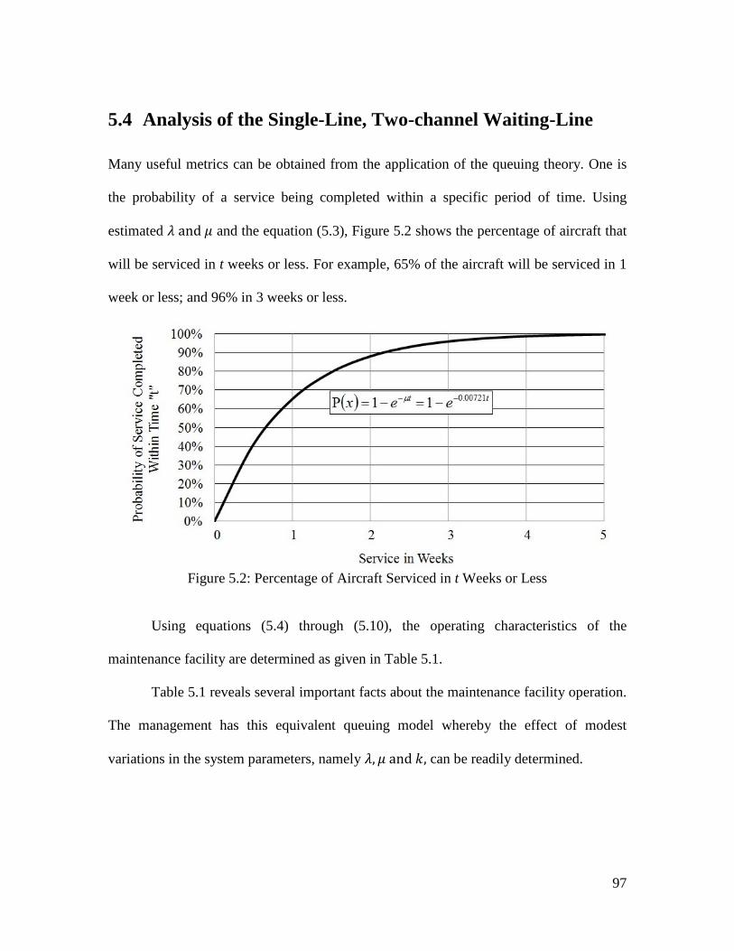
5.4 Analysis of the Single-Line, Two-channel Waiting-Line
Many useful metrics can be obtained from the application of the queuing theory. One is
the probability of a service being completed within a specific period of time. Using
estimated 𝜆 and 𝜇 and the equation (5.3), Figure 5.2 shows the percentage of aircraft that
will be serviced in t weeks or less. For example, 65% of the aircraft will be serviced in 1
week or less; and 96% in 3 weeks or less.
Figure 5.2: Percentage of Aircraft Serviced in t Weeks or Less
Using equations (5.4) through (5.10), the operating characteristics of the
maintenance facility are determined as given in Table 5.1.
Table 5.1 reveals several important facts about the maintenance facility operation.
The management has this equivalent queuing model whereby the effect of modest
variations in the system parameters, namely 𝜆, 𝜇 and 𝑘, can be readily determined.
97

It was pointed out in section 6.3 that the overall mean service rate, 𝑘𝜇, must be
greater than the mean arrival rate, λ. If this condition is not met, the waiting-line
eventually grows infinitely large. Table 5.1 indicates that this condition is well satisfied.
Table 5.1: ISS Engine Maintenance Queuing Model Characteristics
Number of arrivals per month (λ) 6.8
Number of units serviced per month per channel (μ) 5.3
Number of service facilities/channels (k) 2
λ /μ 1.28
P0 0.28
Lq 1.13
L 2.47
Wq 122.68 (hrs)
W 261.01 (hrs)
Pw 0.64
𝑘𝜇 > 𝜆 10.6 > 6.8
Figure 5.3 is a graph of the probabilities of certain numbers of aircraft in the
system. For example, there is a 36% chance there are 2 aircraft in the system, and the
probability that greater than 10 aircraft are in the system is insignificant.
98
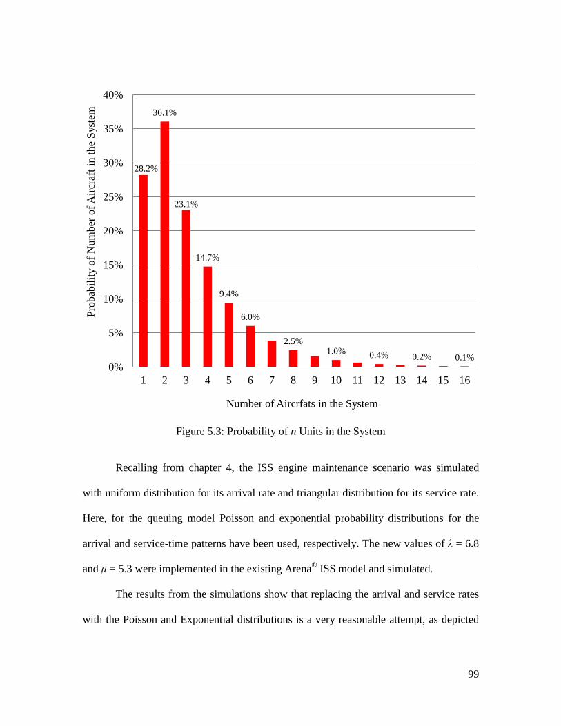
Figure 5.3: Probability of n Units in the System
Recalling from chapter 4, the ISS engine maintenance scenario was simulated
with uniform distribution for its arrival rate and triangular distribution for its service rate.
Here, for the queuing model Poisson and exponential probability distributions for the
arrival and service-time patterns have been used, respectively. The new values of λ = 6.8
and μ = 5.3 were implemented in the existing Arena® ISS model and simulated.
The results from the simulations show that replacing the arrival and service rates
with the Poisson and Exponential distributions is a very reasonable attempt, as depicted
28.2%
36.1%
23.1%
14.7%
9.4%
6.0%
2.5% 1.0% 0.4% 0.2% 0.1%
0%
5%
10%
15%
20%
25%
30%
35%
40%
1 2 3 4 5 6 7 8 9 10 11 12 13 14 15 16
Prob
abili
ty o
f Num
ber o
f Airc
raft
in th
e Sy
stem
Number of Aircrfats in the System
99

in Table 5.2. In particular, it is shown that the percentage difference between the two sets
of results is within an acceptable range.
Table 5.2: Comparison of Different ISS Models
Uniform and Triangular
Distribution (1)
Queuing Theory (2)
Poisson and Exponential Distribution
Percentage Difference between
(1) and (2)
Lq 1.29 1.13 1.05 12.10%
L N/A 2.41 2.33 N/A
Wq (hrs) 108.84 122.68 114.68 12.72%
W (hrs) 247.48 261.01 259.01 5.47%
From Table 5.2, it is concluded that with queuing theory, the effect of modest
change in decision parameters on system performance can be assessed.
100

Chapter 6: Conclusions and Future Work
6 Conclusions and Future Work
6.1 Summary
The objectives of the work presented were to develop decision making support tools and
to assess different aircraft engine maintenance policies. Four preliminary models, one
integrated comprehensive model, four confirmatory models for the verification of the
preliminary models, and one queuing-theory-based equivalent model of the integrated
model were developed. The preliminary models and their simulation provided initial
insight and useful information about the behaviour of the maintenance operation, and
later became parts of the integrated model. The integrated model can be reused and
modified to investigate major changes to the aircraft fleet and maintenance facility
operation. The equivalent queuing model is an easy to use tool for the management to
101

conveniently assess modest changes in the fleet and maintenance facility. These include
for example, increasing service the rate by adding technician and equipment, or
increasing the arrival rate by operating a larger fleet.
6.2 Discussions
From the simulations the following major results were obtained.
1) Although ‘fixed’ inflexible policies are undesirable, but if a choice has to be
made amongst the four preliminary fixed policies, the 2-Engine policy
prevails. Lowest total and average grounding and waiting times, and shorter
average queue length are the desirable performance indicators for this policy.
It is postulated that despite randomness in flying times, since there are even
number of engines (two pairs) on each aircraft, pair-wise engine service drives
the system into a favourably synchronized and alternating service cycles
between the two pairs of the engines resulting in prolonged uninterrupted
flying periods in between.
2) The flexible ISS policy is indeed recommended as it is developed to work
optimally, and has parameters that allow further optimization through multiple
simulations. In the ISS model, the 2-Engine policy was also dominant and
confirmed the earlier findings.
3) The equivalent queuing model reproduced satisfactory results, and proved that
indeed, it can assist in management decision making when minor system
modifications are intended.
102

6.3 Conclusions
From this study a number of important conclusions are drawn. It was shown that
Discrete Event Simulation (DES) software provided significant capability for open-ended
systems modeling where practically any degree of detail, constraints and conditions, both
quantitative and qualitative can be implemented. Despite great utility however, using
DES software or languages is not without challenges. One is their slow rising learning
curve. Their essentially non-mathematical paradigm and modeling construct, such as
entities, attributes, events, resources, and how simulations run, are unfamiliar concepts
even to engineers, who most often are amongst the primary users of DES. The second is
that DES models are dominantly data-driven, and availability of reliable input data is
paramount in successful simulations. As in this study data was not abundantly and readily
available, a good portion of time was spent to extract data from the limited engine
monitoring logs.
The final challenge in using DES is that when real system performance data is
unavailable for validation of the models, as was the case in this study, and this is not
uncommon when a new real system is being developed for example, careful modeling
and greater effort is put on verification to ensure the correctness of the models built.
In this way, overall, satisfactory results and verifications were obtained and tools
were developed to support management in their maintenance policy decision making.
103

6.4 Suggestions for Future Work
The following suggestions may be considered as possible future work for the
enhancement of optimal aircraft maintenance planning.
1. Modeling of the operation of the maintenance facility was carried out in isolation
from aircraft flight schedules and commitments. In fact, at the time when a
decision is made that an aircraft must be dispatched for service, it could be at a
remote location. Therefore, it may be more practical that the aircraft are sent for
service when they are geographically close to the maintenance facility.
Alternatively, if an aircraft is to fly to a distant location, it should be considered in
maintenance time decision making whether upon return of the aircraft the ‘safe
remaining flying time’ still remains. In other words, the set service time threshold
is not violated.
2. A user-friendly front-end graphical interface can be developed to facilitate the use
of the ISS model so as to facilitate and expedite modification and inclusion of
major changes to the operating system in the model.
104

Bibliography
[1] Mishra, R., and Pathak, K., 2004, "Maintenance Engineeering and Management,"
PHI Learning Pvt. Ltd., New Delhi, India, pp. 220.
[2] Geraerds, W., 1985, "The Cost of Downtime for Maintenance: Preliminary
Considerations," Maint.Manage.Int., 5(1) pp. 13-21.
[3] Mobley, R.K., 2011, "Maintenance Fundamentals," Butterworth-Heinemann,
Burlington, USA, pp. 418.
[4] Endrenyi, J., Aboresheid, S., Allan, R. N., 2001, "The Present Status of Maintenance
Strategies and the Impact of Maintenance on Reliability," IEEE Transactions on Power
Systems, 16(4) pp. 638-646.
[5] Sullivan, G., Pugh, R., Melendez, A. P., 2010, "Operations & Maintenance Best
Practices - A Guide to Achieving Operational Efficiency," pp. 321.
[6] King, F.H., 1986, "Aviation Maintenance Management," SIU Press.
[7] Razavi, B., and Sassani, F., 2013, "Aircraft Fleet Maintenance Planning Using
Combined Cost Benefit Model and Branch and Bound," ASME International Mechanical
Engineering Congress and Exposition, IMECE, November 15 - 21. American Society of
Mechanical Engineers (ASME), San Diego, CA, USA, 1, pp. 26-32.
105

[8] Naylor, J., 2002, "Introduction to Operations Management," Pearson Education,
Essex, England, pp. 575.
[9] Tsang, A. H. C., 1995, "Condition-Based Maintenance: Tools and Decision Making,"
Journal of Quality in Maintenance Engineering, 1(3) pp. 3-17.
[10] Rong, X., Zuo, H., and Chen, Z., 2010, "Civil Aero-Engine Health Management
Integrating With Life Prediction And Maintenance Decision Making," Prognostics and
System Health Management Conference, January 12-14. IEEE Computer Society,
Macau, China, pp. 1-6.
[11] Maity, A., Zaremby, D., McMullen, D., 2011, "Automated Scheduling using
Condition Based Maintenance," IEEE International Conference on Prognostics and
Health Management, PHM , June 20 - 23, Association for Computing Machinery,
Denver, CO, USA, pp. 1-8.
[12] Halasz, M., Dubé, F., Orchard, R., 1999, "The Integrated Diagnostic System (IDS):
Remote Monitoring and Decision Support for Commercial Aircraft-Putting Theory into
Practice," Proceedings of the AAAI’99 Spring Symposium on AI in Equipment
Maintenance, AAAI, Canada, pp. 88-94.
[13] Wang, Y., and Liu, X., 2010, "Fuzzy Analytical Hierarchy Process Application in
Safety Risk Management of Aviation Maintenance Process," International Conference on
Management and Service Science, MASS, August 24-26. IEEE Computer Society,
106

Wuhan, China, pp. IEEE Wuhan Section; Sichuan University; Wuhan University; James
Madison University.
[14] Rad, T., Shanmugarajan, N., and Wahab, M. I. M., 2011, "Classification of Critical
Spares for Aircraft Maintenance," 8th International Conference on Service Systems and
Service Management, June 25 -27, 2011, IEEE Computer Society, Tianjin, China, pp.
IEEE Systems, Man and Cybernetics Society; Tsinghua University, Research Center for
Contemporary Management; The Chinese University of Hong Kong; Nankai University.
[15] Altuger, G., and Chassapis, C., 2009, "Multi Criteria Preventive Maintenance
Scheduling Through Arena Based Simulation Modeling," Winter Simulation Conference,
WSC, December 13-16. Institute of Electrical and Electronics Engineers Inc, Austin, TX,
USA, pp. 2123-2134.
[16] Roemer, M. J., Byington, C. S., Kacprzynski, G. J., 2006, "An Overview of
Selected Prognostic Technologies with Application to Engine Health Management,"
ASME 51st Turbo Expo, May 6-11. American Society of Mechanical Engineers,
Barcelona, Spain, 2, pp. 707-715.
[17] OSIsoft, 2007, "Condition-based Maintenance (CBM) Across the Enterprise,"
OSIsoft, Inc., 1, San Leandro, CA.
[18] Kothamasu, R., Huang, S. H., and Verduin, W. H., 2006, "System Health
Monitoring and Prognostics - A Review of Current Paradigms and Practices,"
International Journal of Advanced Manufacturing Technology, 28(9) pp. 1012-1024.
107

[19] Swanson, L., 2001, "Linking Maintenance Strategies to Performance," International
Journal of Production Economics, 70(3) pp. 237-244.
[20] Mobley, R.K., 2002, "An Introduction to Predictive Maintenance," Butterworth-
Heinemann, MA. USA, pp. 438.
[21] Al-Najjar, B., and Alsyouf, I., 2003, "Selecting the most Efficient Maintenance
Approach using Fuzzy Multiple Criteria Decision Making," International Journal of
Production Economics, 84(1) pp. 85-100.
[22] Rosqvist, T., Koski, K., and Siljander, A., 2006, "Fatigue Analysis Framework For
Fleet Management Using Bayesian Networks," Annual Reliability and Maintainability
Symposium, RAMS'06, January 23 - 26, Institute of Electrical and Electronics Engineers
Inc, Newport Beach, CA, United states, pp. 133-139.
[23] Rosqvist, T., Laakso, K., and Reunanen, M., 2009, "Value-Driven Maintenance
Planning for a Production Plant," Reliability Engineering and System Safety, 94(1) pp.
97-110.
[24] Waeyenbergh, G., and Pintelon, L., 2004, "Maintenance Concept Development: A
Case Study," International Journal of Production Economics, 89(3) pp. 395-405.
[25] Waeyenbergh, G., and Pintelon, L., 2009, "CIBOCOF: A Framework for Industrial
Maintenance Concept Development," International Journal of Production Economics,
121(2) pp. 633-640.
108

[26] Wang, L., Chu, J., and Wu, J., 2007, "Selection of Optimum Maintenance Strategies
Based on a Fuzzy Analytic Hierarchy Process," International Journal of Production
Economics, 107(1) pp. 151-163.
[27] Rajamani, R., Wang, J., and Jeong, K., 2004, "Condition-Based Maintenance for
Aircraft Engines," 2004 ASME Turbo Expo, June 14, 2004 - June 17, American Society
of Mechanical Engineers, Vienna, Austria, 2, pp. 819-823.
[28] Chilcott, J. B., and Christer, A. H., 1991, "Modelling of Condition Based
Maintenance at the Coal Face," International Journal of Production Economics, 22(1) pp.
1-11.
[29] Jiang, R., and Jardine, A. K. S., 2008, "Health State Evaluation of an Item: A
General Framework and Graphical Representation," Reliability Engineering and System
Safety, 93(1) pp. 89-99.
[30] Mckone, K. E., and Weiss, E. N., 2002, "Guidelines for Implementing Predictive
Maintenance," Production and Operations Management, 11(2) pp. 109-124.
[31] Jardine, A.K.S., and Tsang, A.H.C., 2006, "Maintenance, Replacement, and
Reliability: Theory and Applications," CRC Press, New York, N.Y., pp. 322.
[32] Jardine, A. K. S., Lin, D., and Banjevic, D., 2006, "A Review on Machinery
Diagnostics and Prognostics Implementing Condition-Based Maintenance," Mechanical
Systems and Signal Processing, 20(7) pp. 1483-1510.
109

[33] Al-Aomar, R., 2000, "Product-Mix Analysis with Discrete Event Simulation,"
Winter Simulation Proceedings, December 10-13, Orlando, FL, USA, 2, pp. 1385-1392.
[34] Knoll, J. M., and Heim, J. A., 2000, "Ensuring the Successful Adoption of Discrete
Event Simulation in a Manufacturing Environment," Winter Simulation Proceedings,
December 10-13, Orlando, FL, USA, 2, pp. 1297-1304.
[35] Dupuy, M. J., Wesely, D. E., and Jenkins, C. S., 2011, "Airline Fleet Maintenance:
Trade-Off Analysis of Alternate Aircraft Maintenance Approaches," IEEE Systems and
Information Engineering Design Symposium, SIEDS, April 29 - 31. IEEE Computer
Society, Charlottesville, VA, USA, pp. 29-34.
[36] Devulapalli, S., Martinez, J. C., and De, l. G., 2002, "Evaluation of Policies for the
Maintenance of Bridges Using Discrete-Event Simulation (DES)," Proceedings of the
Winter Simulation Conference, December 8-11. Institute of Electrical and Electronics
Engineers Inc, San Diego, CA, USA, 2, pp. 1759-1764.
[37] Van, D. B., De Bruecker, P., Belien, J., 2013, "A Three-Stage Approach for Aircraft
Line Maintenance Personnel Rostering using MIP, Discrete Event Simulation (DES) and
DEA." Expert Systems with Applications, 40(7) pp. 2659-2668.
[38] Bazargan, M., and McGrath, R. N., 2003, "Discrete Event Simulation (DES) to
Improve Aircraft Availability and Maintainability." The International Symposium on
Product Quality and Integrity; Transforming Technologies for Reliability and
110

Maintainbility Engineering, January 27-30. Institute of Electrical and Electronics
Engineers Inc, Tampa, FL, USA, pp. 63-67.
[39] Chong, C. S., Sivakumar, A. I., and Gay, R., 2003, "Simulation-Based Scheduling
for Dynamic Discrete Manufacturing," Proceedings of Simulation Conference: Driving
Innovation, December 7-10, Institute of Electrical and Electronics Engineers Inc, New
Orleans, LA, USA, 2, pp. 1465-1473.
[40] Johansson, B., and Kaiser, J., 2002, "Turn Lost Production into Profit - Discrete
Event Simulation (DES) Applied on Resetting Performance in Manufacturing Systems,"
Proceedings of the Winter Simulation Conference, December 8-11, Institute of Electrical
and Electronics Engineers Inc, San Diego, CA, USA, 2, pp. 1065-1072.
[41] Ho, Y., 1989, "Introduction to Special Issue on Dynamics of Discrete Event
Systems," Proceedings of the IEEE, 77(1) pp. 3-6.
[42] Wainer, G.A., 2010, "Discrete-Event Modeling and Simulation: A Practitioner's
Approach," CRC Press, NW, USA, pp. 494.
[43] Patrick, R., Smith, M. J., Byington, C. S., 2011, "Use of Fleet Data and Seeded
Fault Testing to Enhance Diagnostic Operations and Provide the Basis for Safe
Prognostics of a Helicopter Bearing," Airworthiness, CMB and HUMS Specialists'
Meeting, February 7 - 9, American Helicopter Society International, Huntsville, AL,
USA, pp. 88-110.
111

[44] Babbar, A., Ortiz, E. M., Syrmos, V. L., 2009, "Advanced Diagnostics and
Prognostics for Engine Health Monitoring," 2009 IEEE Aerospace Conference, March 7,
2009 - March 14, IEEE Computer Society, Big Sky, MT, United states, .
[45] Byington, C. S., Roemer, M. J., Kacprzymki, G. J., 2002, "Prognostic
Enhancements to Diagnostic Systems for Improved Condition-Based Maintenance
[Military Aircraft]," IEEE Aerospace Conference, March 9 - 16, IEEE Computer Society,
Big Sky, MT, United states, 6, pp. 2815-2824.
[46] Razavi, B., and Sassani, F., 2014, "Optimal Aircraft Engine Maintenance Planning
Using Discrete Event Simulation," BC Chemical & Biological Engineering’s Research
Day, UBC, University of British Columbia, Vancouver, Canada, .
[47] Langer, R., Li, J., Biller, S., 2010, "Simulation Study of a Bottleneck-Based
Dispatching Policy for a Maintenance Workforce," International Journal of Production
Research, 48(6) pp. 1745-1763.
[48] Jarvis, W. J., and Bancroft, M. S., 1980, "Maintenance Planning Scheduling in a
Petro-Chemical Manufacturing Environment," National Petroleum Refiners Association
(Technical Papers).
[49] Chase, R. B., Jacobs, F. R., Aquilano, N. J., 2006, "Operations Management for
Competitive Advantage," pp. 806.
[50] Banks, J., Carson, J., Nelson, B., 2011, "Simulation," 2013(July/10) pp. 6.
112
[51] Oyarbide-Zubillaga, A., Goti, A., and Sanchez, A., 2008, "Preventive Maintenance
Optimization of Multi-Equipment Manufacturing Systems by Combining Discrete Event
Simulation and Multi-Objective Evolutionary Algorithms," Production Planning and
Control, 19(4) pp. 342-355.
[52] Sharda, B., and Bury, S. J., 2008, "A Discrete Event Simulation Model for
Reliability Modeling of a Chemical Plant," Winter Simulation Conference, December 7-
10, Institute of Electrical and Electronics Engineers Inc, Miami, FL, USA, pp. 1736-
1740.
[53] Ahner, D. K., Buss, A. H., and Ruck, J., 2006, "Assignment Scheduling Capability
for Unmanned Aerial Vehicles - A Discrete Event Simulation With Optimization in the
Loop Approach to Solving a Scheduling Problem," 2006 Winter Simulation Conference,
WSC, December 3-6, 2006, Institute of Electrical and Electronics Engineers Inc,
Monterey, CA, United states, pp. 1349-1356.
[54] Gupta, P., Bazargan, M., and McGrath, R. N., 2003, "Simulation Model for Aircraft
Line Maintenance Planning," The International Symposium on Product Quality and
Integrity; Transforming Technologies for Reliability and Maintainbility Engineering,
January 27-30, 2003, Institute of Electrical and Electronics Engineers Inc, Tampa, FL,
United states, pp. 387-391.
113
[55] Duffuaa, S. O., Ben-Daya, M., Al-Sultan, K., 2001, "A Generic Conceptual
Simulation Model for Maintenance Systems," Journal of Quality in Maintenance
Engineering, 7(3) pp. 207-219.
[56] Joo, S. J., Levary, R. R., and Ferris, M. E., 1997, "Planning Preventive Maintenance
for a Fleet of Police Vehicles using Simulation," Simulation, 68(2) pp. 93-100.
[57] Sun, Y., 1994, "Simulation for Maintenance of an FMS: An Integrated System of
Maintenance and Decision-Making," International Journal of Advanced Manufacturing
Technology, 9(1) pp. 35-39.
[58] Cobb, R., 1995, "Modeling Aircraft Repair Turntime: Simulation Supports
Maintenance Marketing Efforts," Journal of Air Transport Management, 2(1) pp. 25-32.
[59] Pannirselvam, G. P., Ferguson, L. A., Ash, R. C., 1999, "Operations Management
Research: An Update for the 1990s," Journal of Operations Management, 18(1) pp. 95-
112.
[60] Ali, A., Chen, X., Yang, Z., 2008, "Optimized Maintenance Design for
Manufacturing Performance Improvement Using Simulation," 2008 Winter Simulation
Conference, S. J. Mason, R. R. Hill, L. Mönch, et al., eds. Piscataway, New Jersey:
Institute of Electrical and Electronics Engineers, Inc., pp. 1811-1819.
[61] Roux, O., Jamali, M. A., Kadi, D. A., 2008, "Development of Simulation and
Optimization Platform to Analyse Maintenance Policies Performances for Manufacturing
114

Systems," International Journal of Computer Integrated Manufacturing, 21(4) pp. 407-
414.
[62] Wikimedia Foundation, I., 2014, "Simulation," 2014(February 6) pp. 8.
[63] Maria, A., 1997, "Introduction to Modeling and Simulation," 29th Winter
Simulation Conference, IEEE Computer Society, pp. 7-13.
[64] Szczerbicki, E., and White, W., 1998, "System Modeling and Simulation for
Predictive Maintenance," Cybernetics and Systems, 29(5) pp. 481-498.
[65] Boehm, B. W., 2013, "Verification and Validation (Software)," 2013(July/23) pp. 2.
[66] Yucel, N. D., 2005, "Simulation of a Flexible Manufacturing System: A Pilot
Implementation," pp. 131.
[67] Takus, D. A., and Profozich, D. M., 1997, "ARENA® Software Tutorial," Winter
Simulation Conference, Sewickley, Pennsylvania, USA, pp. 541-543.
[68] Bahtiyar, M., 2005, "Simulation Modelling of Shop Floor Activities for SMEs in
Virtual Enterprises," pp. 162.
[69] Liu, Y., and Takakuwa, S., 2009, "Simulation-Based Personnel Planning for
Materials Handling at a Cross-Docking Center Under Retail Distribution Environment,"
Winter Simulation Conference, IEEE, Austin, TX, pp. 2414-2425.
115

[70] Chin, S. Y., and Junior, J., 2007, "Modeling and Simulation of Retrieving Process,"
Winter Simulation Conference, IEEE, Washington, D.C., USA, pp. 1682-1690.
[71] Kelton, W.D., Sadowski, R.P., and Sadowski, D.A., 2002, "Simulation with
ARENA," McGraw-Hill, New York, USA, pp. 700.
[72] Birtwistle, G.M., Birtwistle, G.M., Birtwistle, G.M., 1979, "DEMOS, a System for
Discrete Event Modelling on Simula," Citeseer.
[73] Nygaard, K., and Dahl, O., 1978, "The Development of the SIMULA Languages,"
ACM, .
[74] Pristker, A.A.B., and Pegden, C.D., 1979, "Introduction to Simulation and SLAM,"
J. Wiley.
[75] Adams, M., Componation, P., Czarnecki, H., 1999, "Simulation as a Tool for
Continuous Process Improvement," Winter Simulation Conference Proceedings,
December 5-8, IEEE, Phoenix, AZ, USA, 1, pp. 766-773.
[76] Hickie, M., and Fowler, J. W., 1999, "Ancillary Effects of Simulation," Winter
Simulation Conference Proceedings, December 5-8, IEEE, Phoenix, AZ, USA, 1, pp.
754-758.
[77] Harrell, C., and Gladwin, B., 2007, "Productivity Improvement in Appliance
Manufacturing," Winter Simulation Conference, December 9-12, Institute of Electrical
and Electronics Engineers Inc, Washington, DC, United states, pp. 1610-1614.
116

[78] McLean, C., and Shao, G., 2003, "Generic Case Studies for Manufacturing
Simulation Applications," Proceedings of the Simulation Conference: Driving
Innovation, December 7-10, Institute of Electrical and Electronics Engineers Inc, New
Orleans, LA, United states, 2, pp. 1217-1224.
[79] Bell, Z. M., and Teague, L. T. C. E., 2014, "Comparison of Army Aviation
Maintenance Methods via Discrete Event Simulation," IEEE Systems and Information
Engineering Design Symposium, April 25 - 26, IEEE Computer Society, Charlottesville,
VA, USA, pp. 277-282.
[80] Yu, T., Scanlan, J. P., Crowder, R. M., 2012, "Approaches to Modeling the Gas-
Turbine Maintenance Process," Journal of Computing and Information Science in
Engineering, 12(1).
[81] Hill, R. R., Mattioda, D., and Garza, R., 2011, "A Simulation Based Analysis of the
B-1B's AN/ALQ-161 Maintenance Process," Winter Simulation Conference, December
11 - 14, Institute of Electrical and Electronics Engineers Inc, Phoenix, AZ, USA, pp.
2547-2558.
[82] Wong, J. S., Scanlan, J. P., and Eres, M. H., 2008, "Modelling the Life Cycle Cost
of Aero-Engine Maintenance," 15th ISPE International Conference on Concurrent
Engineering, August 18 - 22, Springer-Verlag London Ltd, Belfast, United kingdom, pp.
233-240.
[83] Petty, N. W., and Dye, S., 2013, "Triangular Distributions," 2014(May 6) pp. 6.
117
[84] Wikimedia Foundation, I., 2014, "Triangular Distributions ," 2014(May 6) pp. 4.
[85] Kleeman, M. P., and Lamont, G. B., 2005, "Solving the Aircraft Engine
Maintenance Scheduling Problem using a Multi-objective Evolutionary Algorithm,"
Third International Conference on Evolutionary Multi-Criterion Optimization, March 9 -
11, Springer Verlag, Guanajuato, Mexico, 3410, pp. 782-796.
[86] Pegden, C. D., and Sturrock, T. D., 2008, "Introduction to Simio," Proceedings of
the Winter Simulation Conference, IEEE, Austin, TX, USA, pp. 229-235.
[87] Pegden, C. D., 2007, "Simio: a New Simulation System Based on Intelligent
Objects," Proceedings of the 39th conference on Winter simulation, IEEE Press,
Piscataway, NJ, USA, pp. 2293-2300.
[88] Yang, C., Luo, L., Ren, Q., 2013, "Using Simio for Laparoscopic
Cholecystectomy(LC) Surgery Simulation," 10th International Conference on Service
Systems and Service Management, ICSSSM, July 17 - 19, IEEE Computer Society, Hong
Kong, China, pp. 769-773.
[89] Zhang, K., Wu, R., Ning, J., 2011, "Using Simio for Wartime Casualty Treatment
Simulation," IEEE International Symposium on IT in Medicine and Education, ITME,
December 9 - 11, IEEE Computer Society, Guangzhou, China, 2, pp. 322-325.
[90] Zheng, Q., Shen, J., Liu, Z., 2011, "Resource Allocation Simulation on Operating
Rooms of Hospital," IEEE 18th International Conference on Industrial Engineering and
118
Engineering Management, IE and EM, September 3 - 5, IEEE Computer Society,
Changchun, China, pp. 1744-1748.
[91] Zheng, Q., Chen, S., Shen, J., 2010, "Simulation Modeling of the Operating Room
Based on Simio," International Conference on Engineering Design and Optimization,
ICEDO, October 28 - 30, Trans Tech Publications, Ningbo, China, 37-38, pp. 1162-1166.
[92] Sagron, R., Grosbard, D., Rabinowitz, G., 2014, "Approximation of Single-Class
Queueing Networks with Downtime-Induced Traffic Variability," Taylor & Francis,
(September 30) pp. 1-17.
[93] Sun, L., Jin, J. G., Lee, D., 2014, "Demand-Driven Timetable Design for Metro
Services," Transportation Research Part C: Emerging Technologies, 46pp. 284-299.
[94] Eiselt, H., and Sandblom, C., 2012, "Operations Research,"Springer, Berline,
Germany, pp. 381-395.
[95] Viswanadham, N., and Narahari, Y., 1992, " Performance Modeling of Automated
Manufacturing System,"Prentice Hall Englewood Cliffs, NJ, New Jersey, USA, pp. 315-
350, Chap. 4.
[96] Kim, S., and Whitt, W., 2014, "Are Call Center and Hospital Arrivals Well
Modeled by Poisson Processes?" Manufacturing and Service Operations Management,
16(3) pp. 464-480.
119

[97] Kim, S., and Whitt, W., 2014, "Choosing Arrival Process Models for Service
Systems: Tests of a Nonhomogeneous Poisson Process," Naval Research Logistics, 61(1)
pp. 66-90.
[98] De, M. X., De, A. A., De, S. J., 2013, "Rate of Occurrence of Failures Based on a
Nonhomogeneous Poisson Process: An Ozone Analyzer Case Study," Environmental
Monitoring and Assessment, 185(2) pp. 1463-1471.
[99] Singh, C. J., and Kumar, B., 2013, "Analysis of State Dependent Bulk Arrival
Unreliable Queueing Model," Inderscience Enterprises Ltd, Olney, Bucks., United
Kingdom, 15, pp. 329-355.
[100] Kim, S., and Whitt, W., 2013, "Using Simulation to Study Statistical Tests for
Arrival Process and Service Time Models for Service Systems," 43rd Winter Simulation
Conference - Simulation: Making Decisions in a Complex World, December 8 - 11, IEEE
Computer Society, Washington, DC, USA, pp. 1223-1232.
[101] Marin, A., and Rota Bul, S., 2014, "Explicit Solutions for Queues with
Exponential Service Time Distribution and Application to Product-Form
Approximations," Performance Evaluation, 81pp. 1-19.
[102] He, X. H., Hu, Z. L., Zhai, X. J., 2014, "Maintenance Policy Model Based on
Time-Variant Reliability," International Conference on Mechatronics Engineering and
Computing Technology, April 9 - 10, Trans Tech Publications, Shanghai, China, 556-
562, pp. 3760-3767.
120

[103] Endharta, A. J., and Yun, W. Y., 2014, "A Preventive Maintenance Policy Based
on System State Information," 20th ISSAT International Conference Reliability and
Quality in Design, August 7 - 9, International Society of Science and Applied
Technologies, Seattle, USA, pp. 51-55.
[104] Prado, S. M., Louzada, F., Rinaldi, J. G., 2013, "A New Distribution for Service
Model With State Dependent Service Rate," 2nd International Conference on Informatics
and Applications, September 23 - 25, IEEE Computer Society, Lodz, Poland, pp. 294-
299.
[105] Shophia Lawrence, A., Sivakumar, B., and Arivarignan, G., 2013, "A Perishable
Inventory System with Service Facility and Finite Source," Applied Mathematical
Modelling, 37(7) pp. 4771-4786.
[106] Yin, M., Angus, J. E., and Trivedi, K. S., 2013, "Optimal Preventive Maintenance
Rate for Best Availability with Hypo-Exponential Failure Distribution," IEEE
Transactions on Reliability, 62(2) pp. 351-361.
[107] Evans, J.R., 1992, "Applied Production and Operations Management,"West
Group, Minneapolis, USA, pp. 778-790, Chap. Supplementary Chapter D.
121
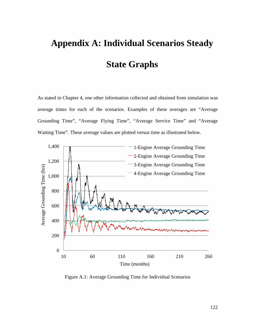
A. Appendix A: Individual Scenarios Steady
State Graphs
As stated in Chapter 4, one other information collected and obtained from simulation was
average times for each of the scenarios. Examples of these averages are “Average
Grounding Time”, “Average Flying Time”, “Average Service Time” and “Average
Waiting Time”. These average values are plotted versus time as illustrated below.
Figure A.1: Average Grounding Time for Individual Scenarios
0
200
400
600
800
1,000
1,200
1,400
10 60 110 160 210 260
Aver
age
Gro
undi
ng T
ime
(hrs
)
Time (months)
___ 1-Engine Average Grounding Time ___ 2-Engine Average Grounding Time ___ 3-Engine Average Grounding Time ___ 4-Engine Average Grounding Time
122
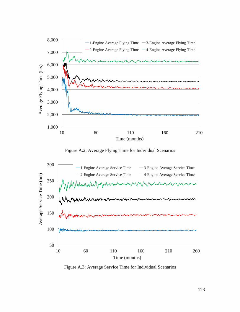
Figure A.2: Average Flying Time for Individual Scenarios
Figure A.3: Average Service Time for Individual Scenarios
1,000
2,000
3,000
4,000
5,000
6,000
7,000
8,000
10 60 110 160 210
Aver
age
Flyi
ng T
ime
(hrs
)
Time (months)
___ 1-Engine Average Flying Time ___ 3-Engine Average Flying Time ___ 2-Engine Average Flying Time ___ 4-Engine Average Flying Time
50
100
150
200
250
300
10 60 110 160 210 260
Aver
age
Serv
ice
Tim
e (h
rs)
Time (months)
___ 1-Engine Average Service Time ___ 3-Engine Average Service Time ___ 2-Engine Average Service Time ___ 4-Engine Average Service Time
123
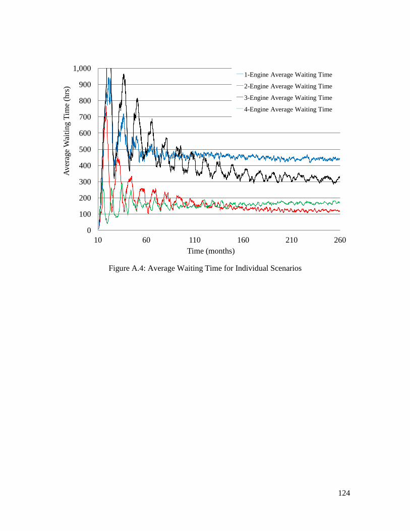
Figure A.4: Average Waiting Time for Individual Scenarios
0
100
200
300
400
500
600
700
800
900
1,000
10 60 110 160 210 260
Aver
age
Wai
ting
Tim
e (h
rs)
Time (months)
___ 1-Engine Average Waiting Time ___ 2-Engine Average Waiting Time ___ 3-Engine Average Waiting Time ___ 4-Engine Average Waiting Time
124

B. Appendix B: ISS Maintenance Steady State
Graphs
In this appendix, the average values for the information collected from simulation in Chapter 4
related to ISS maintenance scenario is illustrated. “Average Grounding Time”, “Average Flying
Time”, “Average Service Time” and “Average Waiting Time” are the examples of these average
values.
Figure B.1: Average Grounding Time for ISS Scenario
0
100
200
300
400
500
600
700
800
10 60 110 160 210 260
Aver
age
Gro
undi
ng T
ime
(hrs
)
Time (months)
125
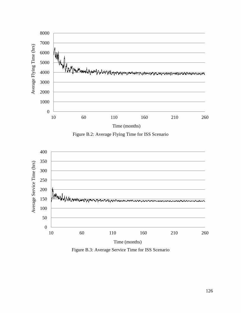
Figure B.2: Average Flying Time for ISS Scenario
Figure B.3: Average Service Time for ISS Scenario
0
1000
2000
3000
4000
5000
6000
7000
8000
10 60 110 160 210 260
Aver
age
Flyi
ng T
ime
(hrs
)
Time (months)
0
50
100
150
200
250
300
350
400
10 60 110 160 210 260
Aver
age
Serv
ice
Tim
e (h
rs)
Time (months)
126

Figure B.4: Average Queue Time for ISS Scenario
0 50
100 150 200 250 300 350 400 450 500 550 600
10 60 110 160 210 260
Aver
age
Que
ue T
ime
(hrs
)
Time (months)
127