decentralized traffic management: a synchronization … filein this paper, we propose a...
TRANSCRIPT

HAL Id: hal-00960735https://hal.inria.fr/hal-00960735
Submitted on 18 Mar 2014
HAL is a multi-disciplinary open accessarchive for the deposit and dissemination of sci-entific research documents, whether they are pub-lished or not. The documents may come fromteaching and research institutions in France orabroad, or from public or private research centers.
L’archive ouverte pluridisciplinaire HAL, estdestinée au dépôt et à la diffusion de documentsscientifiques de niveau recherche, publiés ou non,émanant des établissements d’enseignement et derecherche français ou étrangers, des laboratoirespublics ou privés.
Decentralized Traffic Management: ASynchronization-Based Intersection Control — Extended
VersionMohamed Tlig, Olivier Buffet, Olivier Simonin
To cite this version:Mohamed Tlig, Olivier Buffet, Olivier Simonin. Decentralized Traffic Management: ASynchronization-Based Intersection Control — Extended Version. [Research Report] RR-8500, IN-RIA. 2014, pp.17. <hal-00960735>

ISS
N0
24
9-6
39
9IS
RN
INR
IA/R
R--
85
00
--F
R+
EN
G
RESEARCH
REPORT
N° 8500March 2014
Project-Team MAIA
Decentralized Traffic
Management:
A Synchronization-Based
Intersection Control
—
Extended Version
Mohamed Tlig , Olivier Buffet , Olivier Simonin


RESEARCH CENTRE
NANCY – GRAND EST
615 rue du Jardin Botanique
CS20101
54603 Villers-lès-Nancy Cedex
Decentralized Traffic Management:
A Synchronization-Based Intersection Control
—
Extended Version
Mohamed Tlig ∗, Olivier Buffet ∗, Olivier Simonin †
Project-Team MAIA
Research Report n° 8500 — March 2014 — 17 pages
Abstract: Controlling the vehicle traffic in large networks remains an important challenge in urban envi-
ronments and transportation systems. Autonomous vehicles are today considered as a promising approach
to deal with traffic control. In this paper, we propose a synchronization-based intersection control mecha-
nism to allow the autonomous vehicle-agents to cross without stopping, i.e., in order to avoid congestions
(delays) and energy loss. We decentralize the problem by managing the traffic of each intersection indepen-
dently from others. We define control agents which are able to synchronize the multiple flows of vehicles
in each intersection, by alternating vehicles from both directions. We present experimental results in sim-
ulation, which allow to evaluate the approach and to compare it with a traffic light strategy. These results
show the important gain in terms of time and energy at an intersection and in a network.
Key-words: Multi-Agent Systems, Vehicle flow synchronization, Autonomous Vehicles, Traffic Simula-
tions
∗ Université de Lorraine / INRIA Nancy, France – [email protected]† CITI-INRIA, INSA de Lyon, France – [email protected]
Gestion décentralisée du Trafic:
Contrôle d’intersections fondé sur la synchronisation
—
Version étendue
Résumé : Contrôler le trafic dans les grands réseaux reste un défi important dans les milieux ur-
bains et les systèmes de transport. Les véhicules autonomes sont aujourd’hui considérés comme une
approche prometteuse pour fluidifier le trafic. Dans cet article, nous proposons un mécanisme de contrôle
d’intersection fondé sur la synchronisation pour permettre aux véhicules-agents autonomes de traverser
sans s’arrêter afin d’éviter les congestions (retards) et la perte d’énergie. Nous décentralisons le prob-
lème en gérant le trafic de chaque intersection indépendamment des autres. Nous définissons des agents
de contrôle qui sont capables de synchroniser les multiples flux de véhicules à chaque intersection, en
alternant les véhicules des deux routes. Nous présentons des résultats expérimentaux mesurés en simula-
tion, lesquels permettent d’évaluer l’approche et de la comparer à une stratégie plus classique basée sur
les feux de circulation. Ces résultats montrent le gain important en termes de temps et d’énergie à une
intersection et dans un réseau.
Mots-clés : Systèmes multi-agents, Synchronisation de flux de véhicules, Véhicules autonomes, Simu-
lation du trafic

Decentralized Traffic Management: A Synchronization-Based Intersection Control 3
1 Introduction
In many real transport systems, congestions are generated at the intersections between the roads [1],
i.e., parts of the space which must be shared by the vehicles. There exist several methods to manage
intersections. The simplest ones generally favor one flow against the other, as traffic lights and "STOP"
signals do. Such events generate delays for the vehicles because they require stopping multiple vehicles
for some time [2]. If the flow of vehicles is important, these local delays can lead to the emergence of
congestions.
This work has been conducted in the context of the InTraDE european project, in which autonomous
vehicles transport containers across a seaport1. Yet, we consider generic road networks with multiple
intersections. Each vehicle follows a pre-determined path along one lane, without turning (changes of
direction are not treated here). The objective is to reduce delays and energy consumption, and more
generally avoid blockings.
Our approach consists in synchronizing the flows so that the vehicles can alternately cross the inter-
section without stopping. This requires (1) adapting the vehicles’ speeds so that the vehicles arrive at
the right time to cross the next intersection without collision, and (2) introducing autonomous control
agents at each intersection to handle incoming vehicles. We show how to derive the algorithm in each
such control agent and the speed profile for each vehicle as a function of the parameters of the problem
(spatial dimensions, default speed, angle between roads...).
We empirically evaluate this approach, taking into account various parameters which come into play,
such as the throughput of vehicles or the range of the control agent. These experiments are also a means
to show how it compares to other approaches. To that end, we consider two metrics: the total delay
accumulated by the vehicles while crossing the intersections, and the energy consumption due to the
speed variations.
This paper is organized as follows. The next section presents the problem of intersections in general,
and existing work. In Section 3 we present the principle of the temporal synchronization of two roads
at an intersection, then explain (i) how to compute the minimum time between two vehicles, and (ii) the
algorithm used by the control agent. Section 4 is devoted to the experimental study –through simulations–
of our model compared to a traditional traffic lights solution. Finally, we discuss the perspectives of this
work in the conclusion.
2 Related Work
In this study, we address the general problem of managing crossing flows of vehicles in road networks.
This problem has been traditionally studied in operations research and queueing theory. It typically
concerns vehicles driven by humans but, with the arrival of new technologies, many works integrating on-
line decisions consider an automatic and real-time control. Several approaches based on communications
and GPS (Global Positioning System) propose to improve existing solutions such as traffic lights. In [3],
the authors propose a new strategy to improve traveling times of public transports. The system is based
on booking phases of green light at every intersection and gives priority to buses that are furthest behind.
In the same context, the authors of [4] propose a strategy that gives priority to buses calculated based on
the progress of each of them (along its route) and also on the progress of the following bus.
Other solutions are interested in fully autonomous vehicle control. They can be classified into two
categories.
Reservation approaches, introduced by Dresner and Stone in [1,5], are based on an agent that manages
an intersection. Each vehicle wanting to cross must book a passage time interval and a route. The
advantage of this approach is that, if several vehicles want to pass and if their paths through the junction
1http://www.intrade-nwe.eu
RR n° 8500

4 Tlig, Buffet & Simonin
do not intersect, then all of them can be satisfied. But, otherwise, it is necessary to give priority to one
vehicle over the others.
The decentralized approach introduced by Rashe and Naumann [6, 7] is based mainly on commu-
nication and negotiation between the vehicles to determine the sequence of passage and exit from the
intersection. This approach is known for its limits, which depend on the number of vehicles trying to
negotiate their passage through the intersection.
3 Intersection Synchronization
3.1 Local Synchronization Approach
In this section we define our approach to synchronize the crossing of vehicle flows at an intersection. Be-
fore describing how it works, we present the type of road network we are working with. We consider road
networks made of roads –with one lane or two opposite lanes– and their intersections. The intersections
(described by Figure 1) allow crossing a road but not turning. Roads can intersect at any angle (we first
consider the case when θ = 90◦, then we generalize).
a
b
c
d1
2
θθ
Figure 1: Intersections with 2 flows (left) and 4 flows (right)
Our approach consists in passing alternately –and without stopping– the vehicles of each road with a
sufficient inter-distance in order to avoid collisions.
For this purpose, each intersection is handled by a control agent. Its main role is to communicate
with the vehicles to manage their passage, allowing them to regulate their speed so as to arrive at the
intersection at the right time. The agent has a limited communication range, which defines the distance
from which it can start interacting with vehicles approaching the intersection.
The following section explains in more details:
• how to determine the period at which the alternation between roads will take place;
• how a control agent, given this period, controls the vehicles close to its intersection.
3.2 Minimum Time Period for Crossing
In this paper, all the vehicles are autonomous and identical. They have a width w, a length l and a default
speed V . The flows are also assumed to be roughly equal on all the lanes of the network.
At first, we focus on the synchronization of two flows A and B to allow their crossing without stop-
ping. We seek to determine the minimum time between two vehicles from the flow A, denoted by T ,
that allows passing one vehicle from flow B between them. This means that, on each lane, the average
period between two consecutive vehicles should be at least T . We distinguish three cases depending on
the crossing angle θ between the two roads: θ = 90◦, θ < 90◦ and θ > 90◦.
Inria

Decentralized Traffic Management: A Synchronization-Based Intersection Control 5
3.2.1 θ = 90◦
The crossing zone is defined by the square corresponding to the space shared by the two roads (see
Figure 2). The time required for a vehicle to cross and leave completely the crossing zone is (l + w)/V .
We deduce the minimum period for passing two vehicles (one from each flow):
T =2(l + w)
V, (1)
and the inter-distance between two vehicles from the same flow is Dmin = T ∗ V − l = 2(l + w)− l =l + 2w (subtracting the length of a vehicle).
l
w
w
l
A
B
Crossing zone
Figure 2: Crossing zone with an angle θ = 90◦
3.2.2 θ < 90◦
In this case, one vehicle can enter the (diamond-shaped) crossing zone before the previous vehicle has
completely left (see Figure 3). To minimize the time between two vehicles, the crossing zone must be
shared by both vehicles from each flow.
A
B
B0
A0
Figure 3: Shared zone when θ < 90◦
We deduce the minimum period for passing two vehicles from each flow (see details in App. A.1):
T =2(
w (1−cos θ)sin θ
+ l)
V. (2)
RR n° 8500

6 Tlig, Buffet & Simonin
3.2.3 θ > 90◦
In this case, there is no (simultaneous) sharing of the crossing zone between vehicles from the two flows.
The minimum period for passing two vehicles from each flow is (see details in App. A.2):
T =2(
w (1+cos θ)sin θ
+ l)
V. (3)
3.2.4 Comments —
T has been determined assuming the maximum possible flows of vehicle. But, if less vehicles are going
through the intersection, this just implies leaving “unused” intervals. Also, in practice, T will be increased
by ǫ, a safety margin of vehicle inter-distance.
3.3 Temporal Synchronization of 2 Roads
3.3.1 Principle —
Knowing the minimal period T , we organize the passage of vehicles each half-period Tc = T/2, i.e.,
one road passing one vehicle at even half-periods (even multiples of Tc), while the odd half-periods
correspond to the other road. Figure 4 illustrates this alternating principle of period Tc.
BA
Control Agent
RR
tAlternate the passage of vehicles
i Tc i+1 Tc i+2 Tc... ...i+n Tc
r0
A A A AB B B B B
Figure 4: Synchronization principle of an intersection
One issue is to ensure that the vehicle agents arrive in crossing zones at the default speed V and at
the right time to be synchronized as desired. This requires a specific synchronization phase prior to each
crossing zone. To that end, we define two radii from the center of an intersection:
• r0 (> 0) the distance within which a vehicle is required to run at the default speed V ; and
• R (> r0) the distance within which an incoming vehicle should adapt its speed to synchronize with
the intersection (speed changes occur between R and r0 before the center).
This defines a specific control zone for an intersection.
For each vehicle, the synchronization requires computing (1) at which half period of the crossing zone
to pass, and (2) how to adapt its speed to be synchronized. As a vehicle agent may not know exactly when
to pass, in particular if there could be conflicts with other vehicles in the same lane, we need to introduce
a control agent at each intersection, which is in charge of determining when each incoming vehicle agent
should pass, and thus needs perceiving and communicating with vehicles within range R.
Inria

Decentralized Traffic Management: A Synchronization-Based Intersection Control 7
3.3.2 Synchronizing Vehicles with an Intersection —
A first observation is that each lane can be handled independently. Note also that a vehicle could ar-
rive earlier or later than its originally predicted arrival time. Yet, rather than searching for the solution
optimizing delays or energy consumption, we decide here to slow down all vehicles.
Considering vehicle agent i entering a control zone at current time t and at default velocity V , its
predicted crossing time at the intersection is ta = t + R/V (forgetting about previous vehicles). The
closest next half-period is numbered ni = ⌈ta/T − p/2⌉, where p = 0 or 1 depending whether i is on an
even or odd road. Knowing that the last used half-period (by previous vehicles) on this lane is numbered
nlast, if nlast ≥ ni, then ni should be set to nlast + 1.
Then, to ensure that vehicle agent i enters the crossing zone at the right time and speed so as to cross
the intersection at time niT + pTc, it should follow a speed profile such as presented on Fig. 5, where the
vehicle (1) slows down (acceleration a1 < 0), (2) then runs at constant speed Vx, and (3) finally speeds
up (acceleration a2 > 0).
0Time
vxa1 a2
ni*T
Speed
δta1 δta2
vδtx
r0
vi
R
Figure 5: Speed profile
The other constraints for this profile are:
• the speed is Vi at the start (6= V if the vehicle has been slowed down by a vehicle in front of him)
and V at the end (as required);
• the total length is R− r0; and
• the total duration is (niT + pTc − r0/V )− t.
In our simplified model, using the maximum acceleration (a2) and deceleration (a1) of the vehicle allows
minimizing the loss of kinetic energy.
Solving this problem leads to solving the following quadratic equation:
Vx2 (
a1 − a22a1a2
) + Vx ((tp − t) +a2Vi − a1V
a1a2)
− (ri − r0)−a2V
2i − a1V
2
2a1a2= 0.
A solution exists only if there is enough space to slow down the vehicle agent as desired. Moreover, we
should verify first if there exist mathematically feasible solutions (∆ ≥ 0), then the physical feasibility of
these solutions, i.e., that the resulting speeds, distances and durations in the speed profile are all positive.
3.3.3 Algorithm —
Algorithm 1 thus shows how the control agent handles a single lane, whose parity is known through a
parameter p ∈ {0, 1}. The algorithm computes for each vehicle its programmed arrival time tp at the
RR n° 8500
8 Tlig, Buffet & Simonin
crossing zone, and the related speed profile (recomputing it regularly to adapt to unexpected delays).
Note also that ni should be computed only the first time vehicle i enters the control zone. Otherwise, due
to small errors, the value ni could change from one iteration to the next. This is achieved by assigning a
default value of ni = −1 when vehicle i is first detected by the control agent, having the control agent
remember ni from one iteration to the next, and computing ni if and only if ni = −1 (line 1).
Algorithm 1: Agent Control of One Lane
Input: lane’s parity int p ∈ [0, 1], current time step tnlast = 01
for each vehicle i perceived at distance r0 < ri < R2
(sorted by increasing distance) do3
Get ri, Vi /* (ni is stored in the control agent’s memory) */4
ta = t+ ri/Vi5
if ni = −1 /* i just entered the control zone */6
then7
ni = ⌈ta/T − p/2⌉8
if ni ≤ nlast then ni = nlast + 19
nlast = ni10
tp = ni ∗ T + p ∗ Tc − r0/V11
Calculate and Send the speed profile to vehicle i12
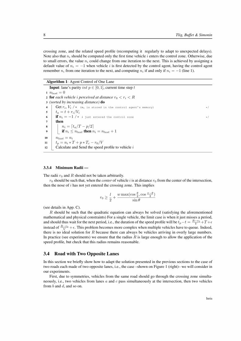
3.3.4 Minimum Radii —
The radii r0 and R should not be taken arbitrarily.
r0 should be such that, when the center of vehicle i is at distance r0 from the center of the intersection,
then the nose of i has not yet entered the crossing zone. This implies
r0 ≥l
2+
wmax(cos θ2 , cos
π−θ2 )
sin θ
(see details in App. C).
R should be such that the quadratic equation can always be solved (satisfying the aforementioned
mathematical and physical constraints) For a single vehicle, the limit case is when it just misses a period,
and should thus wait for the next period, i.e., the duration of the speed profile will be tp−t = R−r0V
+T+ǫ
instead of R−r0V
+ǫ. This problem becomes more complex when multiple vehicles have to queue. Indeed,
there is no ideal solution for R because there can always be vehicles arriving in overly large numbers.
In practice (see experiments) we ensure that the radius R is large enough to allow the application of the
speed profile, but check that this radius remains reasonable.
3.4 Road with Two Opposite Lanes
In this section we briefly show how to adapt the solution presented in the previous sections to the case of
two roads each made of two opposite lanes, i.e., the case –shown on Figure 1 (right)– we will consider in
our experiments.
First, due to symmetries, vehicles from the same road should go through the crossing zone simulta-
neously, i.e., two vehicles from lanes a and c pass simultaneously at the intersection, then two vehicles
from b and d, and so on.
Inria

Decentralized Traffic Management: A Synchronization-Based Intersection Control 9
l
w
Rr0
Control
Agent
Figure 6: Radii R and r0
The minimum period T for crossing must be adjusted to this specific case to account for (i) the size
of the new crossing zone, and (ii) the synchronization pattern the vehicles should follow. Let λ be the
distance separating two opposite lanes of the same road (see Fig. 7). The minimum period is (see details
in App. B):
T =2(
2(w+λ
2)
sin θ+ l)
V. (4)
Furthermore, we should adapt the radius r0 to this configuration. Thus, instead of using the width wof a vehicle as the width of the road, we will consider the width of a two-lane road.
The control agent’s algorithm is unchanged, each lane being handled independently of the other lanes,
e.g., each lane having its own nlast variable. One should just pay attention to the fact that, for a given
lane, distances are not computed with respect to the center of the crossing zone, but with respect to the
middle of the lane’s segment inside the crossing zone, as illustrated on Figure 7.
θ
λ
Figure 7: Crossing zone in the case of 2 opposite lanes in each road
4 Experimental Results
In this section we evaluate our approach on a network of three roads organized as a triangle, giving results
for a single intersection between two two-lane roads, as in Figure 8, before considering more complex
networks.
We compare our approach to a strategy based on traffic lights with a fixed time for each cycle. A
traffic light is placed at the entrance of each flow of the intersection. The lights can switch the passage of
vehicles between two roads, for fixed (equal) periods.
4.1 Simulations
We have developed (in JAVA) a continuous-space and discrete-time simulator of a network of roads.
The detailed experimental setting for our three-road network is the following:
• roads are 1000m long and the angle of the intersection is π3 ;
RR n° 8500

10 Tlig, Buffet & Simonin
Figure 8: Simulator : illustration of an intersection control
• the control agents’ range of action R is 200m and r0 = 30m;
• the maximum speed of each vehicle is 10m/s, the maximum acceleration is 1.5m/s2 and the
maximum deceleration is −1.5m/s2;
• we used a near-to-near longitudinal control developed in [8], which ensures a collision-free behav-
ior between the same lane vehicles (only outside the control zone);
• at each entrance of the network, we installed a source that generates vehicles following a Bernoulli
distribution with parameter 1D
(D is the average time, in seconds, between two consecutive injec-
tions);
• the vehicles have dimension l = 5m, w = 2.5m and safety margin of vehicle inter-distance
ǫ = 1.5m;
• Simulation time step is set to 0.1s.
In this case, the minimum period is T = 3.2s.
For the traffic lights approach, we can fix the green and red times for each flow. We vary their duration
in the following subsection but the reference value is equal to 30s for each color. The green lights of the
same road are turned on at the same time.
4.2 Comparing Various Strategies
Our objective is to compare our approach with traffic lights by observing the resulting delays —i.e., the
difference between the theoretical and actual traversal times— when 100 vehicles traverse the network
under a high injection frequency (D = 4s), i.e., heavy traffic.
Figure 9 presents simulation results for our algorithm and traffic lights with different durations (10s,
20s, 30s). The X axis represents the number of vehicles having left the network in their output order and
the Y axis gives the vehicle’s average delay in seconds (plus standard deviation) over 100 simulations.
Our approach is clearly more efficient in this experiment compared to traffic lights. Here, the worst
delay produced by a vehicle with the local synchronization approach does not exceed 6s, while for traffic
lights it exceeds 20s (maximum value with the standard deviations using 30s duration). The average
delay is below 4s for the local synchronization while, for the best traffic lights curve, it is around 9s(using 10s or 20s duration). We also tested the traffic lights strategy with less than 10s duration and we
observed that the average delay increases significantly. This is mainly due to vehicles requiring more time
to traverse an intersection when they have to restart, which even leads to queue formations and collisions
at or below 5s.
Inria

Decentralized Traffic Management: A Synchronization-Based Intersection Control 11
0
5
10
15
20
25
0 10 20 30 40 50 60 70 80 90 100
Dela
y (
seconds)
Number of vehicles having left the network
Traffic lights 30Traffic lights 20Traffic lights 10
Synchronization T=3,2s
Figure 9: Synchronization vs. Traffic lights
4.3 Effect of Varying R
In this section, we measure the effect of varying the range of action R of the control agent to evaluate
whether this influences the quality of our solution (without modifying r0). Table 1 gives the averages
and the standard deviations of the energy consumed when R = 50m, R = 100m and R = 200m. This
consumed energy is measured through the total change in velocity during the travel of 1000 vehicles. We
observe that the delays do not change significantly, but there is a difference in terms of energy consumed
when we reduce the crossing zone. It increases when we use a small R. This is due to the small distance
that forces the control agent to slow down the vehicles suddenly.
Table 1: Averages and Standard Deviations of the Energy Consumed
D = 10s 50m 100m 200m
Average Energy 8.6 5.2 4Standard Deviation ±3.1 ±3.84 ±4.6
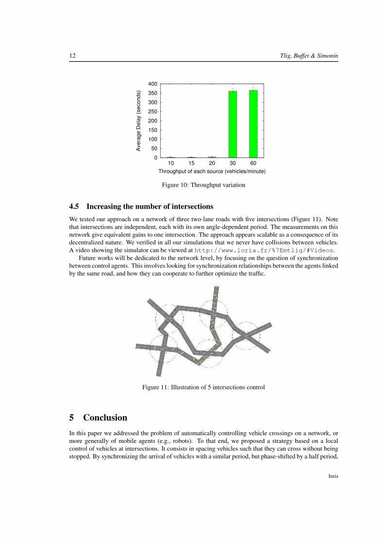
4.4 Effect of Varying D
We want to see here if our approach is efficient when the vehicles’ throughput is higher (generally the
reservation based approaches, as in [1], have poor resistance). Figure 10 shows the variations of delays
depending on the injection throughputs. The plotted histograms are averages of 10000 vehicles. We used
D with the values 1s, 2s, 3s, 4s and 6s which correspond respectively to the throughputs 60, 30, 20,15and 10 vehicles/minute for each source. According to the figure, the average delay increases slightly
(less than 1s) when the throughput is less than the minimal period of the intersection (3.2s). Immediately
thereafter (using 30veh/m and 60veh/m) we saturate the system, as also observed by [1].
RR n° 8500
12 Tlig, Buffet & Simonin
0
50
100
150
200
250
300
350
400
10 15 20 30 60
Ave
rag
e D
ela
y (
se
co
nd
s)
Throughput of each source (vehicles/minute)
Figure 10: Throughput variation
4.5 Increasing the number of intersections
We tested our approach on a network of three two-lane roads with five intersections (Figure 11). Note
that intersections are independent, each with its own angle-dependent period. The measurements on this
network give equivalent gains to one intersection. The approach appears scalable as a consequence of its
decentralized nature. We verified in all our simulations that we never have collisions between vehicles.
A video showing the simulator can be viewed at http://www.loria.fr/%7Emtlig/#Videos.
Future works will be dedicated to the network level, by focusing on the question of synchronization
between control agents. This involves looking for synchronization relationships between the agents linked
by the same road, and how they can cooperate to further optimize the traffic.
Figure 11: Illustration of 5 intersections control
5 Conclusion
In this paper we addressed the problem of automatically controlling vehicle crossings on a network, or
more generally of mobile agents (e.g., robots). To that end, we proposed a strategy based on a local
control of vehicles at intersections. It consists in spacing vehicles such that they can cross without being
stopped. By synchronizing the arrival of vehicles with a similar period, but phase-shifted by a half period,
Inria

Decentralized Traffic Management: A Synchronization-Based Intersection Control 13
vehicles from both flows pass alternately. Therefore the vehicles potentially face a slight slow-down in
order to be able to cross the intersection, which is better than stopping them.
Based on this principle, we defined a crossroad/intersection agent at each intersection which uses only
its local perceptions of the traffic. It determines the instructions for each vehicle to cross the intersection
based on its distance and on the parity assigned to the road. The experimental study demonstrated the
ability to regulate the traffic at intersections, and the significant gain in terms of time compared to a
conventional traffic lights system.
Future work includes first continuing the experimental study to test the limits of our approach and
further evaluate it in a wide variety of scenarios. The other perspective that motivates our research is
to let the control agents communicate and synchronize with each other in order to further improve the
traffic on the network, typically by inducing green waves. As these synchronization constraints involve
neighboring intersections, locally interacting control agents could find a globally efficient solution.
A Calculation of the minimum period for two flows
A.1 Case θ < 90◦
We consider two flows A and B. The crossing order of the vehicles is A0, B0, A1, B1, A2, B2... (see
Figure 12).
l
wθ
θθ w
w
l1
l2
l3
l3
A
B
B0
A0
l
w
A1
Figure 12: Synchronization of two flows with an angle θ < 90◦
For each vehicle we will consider two situations:
• when a vehicle starts to leave the crossing zone (e.g., A0 in Figure 2-b),
• and when a vehicle continues to enter the crossing zone (e.g., B0 in Figure 2-b),
From these two cases, we will –using Figure 12 (which introduces the distances l1, l2, l3)– determine
the minimum time period. To that end, let us observe the evolution of the vehicles:
• at t = 0, A0 starts leaving, B0 continues entering;
• at t = (w2 + l)/V , B0 starts leaving, A1 continues entering;
• at t = [(w2 + l) + (w2 + l)]/V , A1 starts leaving, B1 continues entering;
• · · ·
RR n° 8500

14 Tlig, Buffet & Simonin
From Figure 12, we can determine l1 = wtan θ
and l3 = wsin θ
, then: l2 = l3 − l1 = wsin θ
− wtan θ
. We
can thus write the period as:
T = 2( w
sin θ−
w
tan θ+ l)
/V
= 2
(
w(1− cos θ)
sin θ+ l
)
/V.
To check this formula, consider the two limit cases when θ = 0 and θ = π2 . If θ goes to 0,
(1−cos θ)sin θ
tends to 0, therefore the period T tends to 2l/V , which is logical because the two flows run in the same
direction. If θ goes to π2 ,
(1−cos θ)sin θ
tends to 1, therefore the period T tends to 2(w + l)/V as in the
formula 1.
A.2 Case θ > 90◦
We consider two flows A and B. The crossing order of the vehicles is A0, B0, A1, B1, A2, B2... (see
Figure 13).
l
w
θ
w
w
l2l3
l3
θ
π-θ
l
w
A
B
A0
B0
A1
Figure 13: Synchronization of two flows with an angle θ > 90◦
For each vehicle we will consider two situations, as in the previous case:
• when a vehicle leaves the crossing zone,
• and when a vehicle enters the crossing zone.
We notice here that there are never two different vehicles in the crossing zone. From these two cases,
we will –based on Figure 13 (which introduces new distances l2, l3)– determine the minimum time period.
Let us again observe the evolution of the vehicles:
• at t = 0, A0 leaves, B0 enters;
• at t = (l3 + l2 + l)/V , B0 leaves, A1 enters;
• at t = [(l3 + l2 + l) + (l3 + l2 + l)]/V , A1 leaves, B1 enters;
• · · ·
From Figure 13 we can determine l3 = wsinπ−θ
= wsin θ
and l2 = l3|cos(π− θ)| = l3|cos(θ)| =w
tan θ.
We can thus write the period as:
T = 2( w
sin θ+
w
tan θ+ l)
/V
= 2
(
w(1 + cos θ)
sin θ+ l
)
/V.
Inria

Decentralized Traffic Management: A Synchronization-Based Intersection Control 15
To check this formula, consider the two limit cases when θ = π2 and θ = π. If θ goes to π
2 ,(1+cos θ)
sin θ
tends to 1, therefore the period T tends to 2(w + l)/V as in formula 1. If θ goes to π,(1−cos θ)
sin θtends to
∞, which is logical because the two flows can not be in opposite directions.
B Calculation of the Minimum Period for Four Flows
Let us consider two crossing roads with two opposite lanes each ((A,C) and (B,D)). Let λ be the dis-
tance between two opposite lanes on one road. The two opposite lanes of a given road should trivially
cross the intersection at the same time, so that the crossing order is (A0, C0), (B0, D0), (A1, C1), (B1, D1)...(Figure 14).
l
w
θ
θ
B0
lw
D0
C0
A0
λ
l1(λ/2)+w
Figure 14: Synchronization of four flows
The crossing zone is now defined by the diamond corresponding to the space shared by the two roads
(see Figure 14). To cross and leave completely the crossing zone, a vehicle spends (2l1 + l)/V time.
From Figure 14, we can determine l1 =w+λ
2
sin θ. Therefore the minimum period is:
T = 2
(
2(w + λ2 )
sin θ+ l
)
/V.
C Calculation of the Minimum Radius r0
Let us consider a vehicle entering an intersection (between two single-lane roads), as illustrated on Fig-
ure 15. This vehicle should be at constant speed V as soon as it enters the diamond. Because the control
agent for this intersection uses a circle of radius r0 to delimit what is inside the intersection, a safe choice
is to set r0 as equal to the longest half-diagonal (d1 or d2) of this diamond. Thus r0 = max(d1, d2). This
longest half-diagonal depends on the angle of the intersection θ.
From Figure 15, we can determine d1 = h cos θ2 and d2 = h cos π−θ
2 , where h = wsin θ
. The length l2
is also added because the reference point of the vehicles is their center of gravity. The minimum radius
r0 is therefore:
r0 =l
2+
wmax(cos θ2 , cos
π−θ2 )
sin θ.
To adapt this formula to two-lane roads, we must consider the entire width of the road –denoted Γ–
instead of considering the width of a vehicle, which leads to the new formula of the minimum radius r0
RR n° 8500

16 Tlig, Buffet & Simonin
A
r0
w
θ/2
θ
d1
d2
h
l/2
Figure 15: Determining the minimum radius r0 (for two single-lane roads)
is:
r0 =l
2+
Γmax(cos θ2 , cos
π−θ2 )
sin θ.
Figure 16 shows the variation of the minimum radius r0 as a function of the crossing angle θ.
0
10
20
30
40
50
60
0 10 20 30 40 50 60 70 80 90 100 110 120 130 140 150 160 170 180
Dis
tance (
mete
rs)
Angle (degrees)
r0
Figure 16: r0 as a function of θ (for two two-land roads, and using the distances specified in the experi-
mental section)
References
[1] K. Dresner and P. Stone, “Multiagent traffic management: A reservation-based intersection control
mechanism,” in Proceedings of the Third International Joint Conference on Autonomous Agents and
Multiagent Systems (AAMAS), 2004.
[2] C. Fok, M. Hanna, S. Gee, T. Au, P. Stone, C. Julien, and S. Vishwanath, “A platform for evaluating
autonomous intersection management policies,” in Third International Conference on Cyber-Physical
Systems (ICCPS). IEEE, 2012, pp. 87–96.
Inria
Decentralized Traffic Management: A Synchronization-Based Intersection Control 17
[3] N. Bhouri, F. Balbo, S. Pinson, and M. Tlig, “Collaborative agents for modeling traffic regulation
systems,” in Web Intelligence and Intelligent Agent Technology (WI-IAT), 2011 IEEE/WIC/ACM In-
ternational Conference on, vol. 2, aug. 2011, pp. 7 –13.
[4] N. Hounsell and B. Shrestha, “A new approach for co-operative bus priority at traffic signals,” Intel-
ligent Transportation Systems, vol. 13, no. 1, pp. 6 –14, 2012.
[5] K. Dresner and P. Stone, “Multiagent traffic management: An improved intersection control mech-
anism,” in Proceedings of the Fourth International Joint Conference on Autonomous Agents and
Multiagent Systems (AAMAS), 2005.
[6] R. Naumann and R. Rasche, Intersection collision avoidance by means of decentralized security and
communication management of autonomous vehicles. Univ.-GH, SFB 376, 1997.
[7] R. Naumann, R. Rasche, J. Tacken, and C. Tahedi, “Validation and simulation of a decentralized
intersection collision avoidance algorithm,” in Intelligent Transportation System (ITSC’97), IEEE,
1997, pp. 818–823.
[8] A. Scheuer, O. Simonin, and F. Charpillet, “Safe longitudinal platoons of vehicles without commu-
nication,” in Proceedings of the international conference on Robotics and Automation (ICRA), 2009,
pp. 2835–2840.
RR n° 8500

RESEARCH CENTRE
NANCY – GRAND EST
615 rue du Jardin Botanique
CS20101
54603 Villers-lès-Nancy Cedex
Publisher
Inria
Domaine de Voluceau - Rocquencourt
BP 105 - 78153 Le Chesnay Cedex
inria.fr
ISSN 0249-6399