dec 2020 - aera.gov.in
TRANSCRIPT
Dec 2020


Dec 2020


1
Table of Contents
1.1. Capital Asset Pricing Model (CAPM) ............................................................................................ 9
1.2. Overview of Airport Sector ............................................................................................................11
1.3. Project Scope and Overview..........................................................................................................12
2.1. Airports’ Economic Regulatory Framework Worldwide ...................................................16
2.2. Comparable Airports (Comparable to BIAL) ..........................................................................21
2.2.1. Capitalization and Ownership Structure .........................................................................27
2.2.2. Funding Mechanism ................................................................................................................32
2.2.3. Trends in Airports Operations’ ...........................................................................................32
2.3. Associated Issues ...............................................................................................................................37
2.3.1. Internal Rate of Return to Equity Investors ...................................................................37
2.3.2. Operators’ Returns: A Case of BIAL Divestment ...........................................................38
2.3.3. Prevalent Trends in other Infrastructure Space ...........................................................39
2.4. Determinants of CoE used in the Comparables’ Set .............................................................40
2.5. Sensitivity of Betas – Indian Scenario .......................................................................................42
2.6. Conclusion ............................................................................................................................................43
3.1. Capital Asset Pricing Model ...........................................................................................................45
3.2. Methodology for CoE Estimation ................................................................................................48
3.2.1. Methodology Summary ..........................................................................................................48
3.2.2. Un-levering the Betas of the Listed firms in the Comparable Airports’ Set .......49
3.2.3. Estimating Asset Betas for BIAL .........................................................................................50
3.2.4. Re-levering the BIAL’s Asset Beta to get Equity Beta .................................................50
3.2.5. Cost of Equity and FRoR .........................................................................................................51
3.3. Results and Discussion ....................................................................................................................52
3.3.1. Shortlisting Relevant Airports for Asset Betas for BIAL ...........................................52
3.3.2. Results Related to Estimating Asset Betas of Airports in the Comparable Set .52
3.3.3. Results Related to Estimation of Asset Betas for BIAL ..............................................53
3.3.4. Re-levering Asset Betas of BIAL ..........................................................................................54

2
3.3.5. Results Related to Estimation of Equity Betas for BIAL ............................................61
3.3.6. Equity Risk Premium ..............................................................................................................62
3.3.7. Risk Free Rate ............................................................................................................................65
3.3.8. Cost of Debt – Illustrative Purpose only ..........................................................................66
3.3.9. Cost of Equity (CoE) and Fair Rate of Return (FRoR) .................................................67
3.3.10. Survey Estimates of Cost of Equity ....................................................................................71
3.4. Conclusion and Final Recommendation ...................................................................................71
3.4.1. Utility for Estimating CoE (and FRoR Computations) ................................................72

3
List of Tables
Table R1: Regulatory Framework Worldwide…………………………………………………………...18-20
Table 2.1: Proximity scores of different airports w.r.t BIAL ............................................................. 24
Table 2.2: Ownership structure of Heathrow Airport ......................................................................... 28
Table 2.3: Ownership structure of Gatwick Airport ............................................................................. 28
Table 2.4: Ownership structure of Sydney Airport ............................................................................... 29
Table 2.5: Ownership structure of Auckland Airport .......................................................................... 29
Table 2.6: Ownership structure of Malaysia Airport Holdings Berhad (MAHB) ....................... 30
Table 2.7: Ownership structure of Bangalore International Airport Ltd. (BIAL) ..................... 31
Table 2.8: Ownership structure of Delhi International Airport Ltd. (DIAL) ............................... 31
Table 2.9: Ownership structure of Mumbai International Airport Ltd. (MIAL) ........................ 32
Table 2.10: Ownership structure of Hyderabad International Airport Ltd. (HIAL) ................. 32
Table 2.11 : Relationship between Revenue Per Passenger vs. EAT (Comparable Set) ......... 36
Table 2.12: Relationship between Revenue per passenger vs. EAT (Indian Airports) ........... 36
Table 2.13: IRR computation for BIAL divestment (All amounts in INR Crore)........................ 39
Table 2.14: Auckland Regulator Betas ....................................................................................................... 41
Table 2.15: Heathrow Regulator Betas ...................................................................................................... 41
Table 2.16: Gatwick Regulator Betas .......................................................................................................... 42
Table 2.17: Dublin Regulator Betas ............................................................................................................ 42
Table 3.1: Asset and Equity Betas for 3 Comparable International Airports ............................. 53
Table 3.2: Regulator Estimated Asset Betas for 3 Comparable International Airports .......... 53
Table 3.3: Asset Betas for BIAL. .................................................................................................................... 54
Table 3.4: Target Gearing Ratios .................................................................................................................. 56
Table 3.5: Number of Infra Companies for MDE to BDE Relation ................................................... 59
Table 3.6: BDE vs. MDE regression results for listed Indian Infrastructure Firms. ................. 60
Table 3.7: Estimation of Cost of Debt (CoD) – For Illustrative Purpose only ............................. 67
Table 3.8: Variables Used to Estimate CoE and FRoR .......................................................................... 68
Table 3.9: Estimation of Cost of Equity (CoE) for BIAL ....................................................................... 69
Table 3.10: Final Recommendations .......................................................................................................... 72

4
List of Figures
Fig 2.1: Airport Proximity Scores w.r.t. Bangalore ................................................................................ 26
Fig 2.2: Passenger Movement Trends ........................................................................................................ 33
Fig 2.3: Revenue Trends .................................................................................................................................. 34
Fig 2.4: Revenue Per Passenger Trends .................................................................................................... 34
Fig 2.5: Earnings after Tax Trends .............................................................................................................. 35
Fig 2.6: Past 5 years’ IRR based on Book and Equity Returns .......................................................... 38
Fig 2.7: Framework for InVITs, ..................................................................................................................... 40
Fig 3.1: Regression Results for Market D/E (MDE) vs. Book D/E (BDE) for Listed
International Airports ............................................................................................................................. 57
Fig 3.2: Regression Results for Market D/E (MDE) vs. Book D/E (BDE) for listed Indian
Infrastructure Firms................................................................................................................................. 59
Fig 3.3: CoE by Sector ....................................................................................................................................... 71
Fig 3.4: Screenshot of User Inputs in Excel Utility ................................................................................ 73
Fig 3.5: Values corresponding to the variables based on user input ............................................. 73
Fig 3.6: Final Output in the Excel Utility.................................................................................................... 73

5
List of Equations
Equation 1.1 – CAPM............................................................................................................................................ 9
Equation 1.2 – Breakeven Returns .............................................................................................................. 12
Equation 2.1 – Operations Scale ................................................................................................................... 22
Equation 2.2 – Passenger Ratio .................................................................................................................... 22
Equation 2.3 – Air Traffic Ratio .................................................................................................................... 22
Equation 2.4 – Cargo Ratio ............................................................................................................................. 22
Equation 2.5 – Proximity Score w.r.t. BIAL .............................................................................................. 23
Equation 3.1 – Unlevering Betas .................................................................................................................. 49
Equation 3.2 – Weighted Avg. Betas ........................................................................................................... 50
Equation 3.3 – Re-levering Betas ................................................................................................................. 51
Equation 3.4 – Fair Rate of Return .............................................................................................................. 51
Equation 3.5 – BDE/ MDE Relation ............................................................................................................. 58
Equation 3.6 – MDE/BDE (Actual) .............................................................................................................. 60
Equation 3.7 – Equity Beta for BIAL ........................................................................................................... 61

6
This page is intentionally left blank

7
Executive Summary
This report provides an estimate of the Cost of Equity (CoE) for Bangalore International
Airport Ltd (BIAL). A benchmark set of “comparable” international airports are used to
estimate the systematic risk exposure of BIAL aero assets under a target gearing ratio, as
described in the Capital Asset Pricing Model (CAPM). The Cost of Equity computation also
accounts for BIAL specific attributes such as revenue till structure, ownership structure and
scale of operations by using a proximity score weighted approach, which factors the
closeness of BIAL to the set of “comparable” airports. Based on a reasonable set of
assumptions, the report provides the following estimates of Cost of Equity:
Variable
(Col 1)
BIAL
(Col 2)
Asset Beta based on Proximity Score
Weights of comparable set 0.564689
Target gearing ratio (Debt/Debt + Equity) 48%
Target gearing ratio (Debt/Equity) 0.9231
Equity Betas 0.9296
Risk Free Rate 7.56%
Equity Risk Premium 8.06%
Cost of Equity 15.05%

8
This page is intentionally left blank
9
Chapter 1 – Introduction
The airport infrastructure sector has been undergoing a phased change during the past 15
years. The first Public Private Partnership (PPP) model of airport operations was
implemented in Delhi, Mumbai, Bangalore and Hyderabad airports starting in 2004. While
Delhi and Mumbai were brownfield projects, the other two were greenfield in nature. As with
any infrastructure project, these projects involved high Capital Expenditure (CAPEX) and
Operational Expenditure (OPEX) mobilization. To ensure viability of airport investment, it is
standard practice to provide a reasonable return to investors by charging airport users an
appropriate tariff.
The Airports Economic Regulatory Authority (AERA) was established in 2008 for fixing aero
tariffs and User Development Fee (UDF) at different airports.1 AERA uses the Capital Asset
Pricing Model (CAPM) to determine the Cost of Equity (CoE) and hence the FRoR. As
mandated by the Act, the tariffs are determined at a periodicity of 5 years. This report
computes the CoE (and illustrates the process to compute FRoR) for the Bangalore
International Airport Ltd. (BIAL).
1.1. Capital Asset Pricing Model (CAPM)
The Capital Asset Pricing Model (CAPM) has evolved and has been used effectively for some
time now across industries the world over. Equation 1.1 depicts the CAPM2
RE = Rf + βE (RM – Rf),
Equation 1.1 – CAPM
where
RE = Expected return (and the company’s cost of equity capital)
Rf = Risk-free rate.
RM - Rf = Equity Risk Premium (ERP).
1http://aera.gov.in as viewed on 30th Nov. 2020. 2 While in our study here, we have used the CAPM model, there are also other models available for exploration. Some of these being, the Arbitrage Pricing Theory and other variants of the CAPM (e.g., Breeden’s Consumption CAPM and Merton’s ICAPM) are theoretically sophisticated models that are more general than the CAPM. However, for all practical purposes, the plain CAPM is by far the most widely accepted model used to estimate the cost of capital.
10
βE = Equity beta.
Various methods are employed for determining Rf, RM and βE. We use this CAPM equation
(Equation 1.1) throughout this report for the computation of Cost of Equity.
The NIPFP study3 commissioned by AERA around 2011 had argued and proposed a rate
between 11.64% and 13.84% as the Cost of Equity. However, the NIPFP study is dated in the
sense that Equity Risk Premiums are time varying and the information set as of 2011 (the
time-period of the NIPFP study) differs from the current information set (as of 2018). As is
evident from Eq. (1), the rate of return or CAPM rate depends on 3 inherent factors.
a. Risk-free rate, Rf
b. Equity Risk Premium (ERP), RM – Rf
c. Equity βE
While it is relatively easy to determine Rf, the other two factors are difficult to estimate in
the case of India. Some estimates of the long-term Equity Risk Premium (ERP), and hence,
long-term expected returns (RM) by Damodaran4 and others5,6 are available in literature. The
equity βE estimation can also yield a range of values depending on the assumptions
employed.
Fair Rate of Return (FRoR)
The Fair Rate of Return (FRoR) is essentially the weighted average cost of capital evaluated
at a normative debt to equity ratio. It reflects the cost of equity and the cost of debt and can
be thought of as the return demanded by the providers of capital (debt and equity holders).
Using an illustrative cost of debt (since cost of debt must be estimated annually using the
latest information), we illustrate the computation of FRoR in Chapter 3 (section 3.3.5 and
Equation 3.4).
3 “Estimating Cost of Capital for Private Airports in India”, NIPFP, Dec 2011 4 http://pages.stern.nyu.edu/~adamodar/ as seen on 10 Sep 2018 5 Dimson, Marsh and Staunton (DMS); Triumph of the Optimists: 101 Years of Global Investment Returns (Princeton University Press, 2002) 6 The Global Finance Data (GFD) from www.globalfinancialdata.com as viewed on 28 Feb 2020

11
1.2. Overview of Airport Sector
Traditionally, airports have been managed by governments the world-over with private
participation limited to fuel farms, cargo handling, etc. However, more recently, with
demanding passengers (looking for better quality infrastructure with contemporary
amenities), private participation has become imperative. It has been observed from
experience in other sectors (e.g., ports, roads, etc.) that this mode of operation maximizes
efficiency. Also, the government gains monetarily by selling its stake. The British Airports
Authority or BAA was the first airport to be publicly listed and traded in 1987.7 However,
owing to high losses triggered by expansions and high operating costs, it finally delisted in
2006. However, other airports like Auckland, Sydney, Thailand (AoT), Malaysia (MAHB), etc.
have consistently been successful.
While privatization brings in efficiency and a level of comfort and luxury to the end user, it
also imposes a cost on them. The cost is mostly levied in the form of tariffs and fees by the
private operator to recoup the CAPEX and OPEX incurred. In order to protect the interests of
the end user, regulatory authorities all over the world cap the tariffs that can be levied. For
this purpose, airports are classified as based on a “Till Model” as follows:8
• Single Till – All airport revenues (including aero and non-aero) are taken into
consideration when determining the level of airport usage charges.
• Dual Till – Only aero revenues are taken into consideration when setting airport
usage charges.
• Hybrid Till – Aero revenues along with a percentage of non-aero revenues are
considered for setting airport usage charges.
Typically, aero revenues include landing and parking charges, aerobridge usage charges,
UDF, fuel throughput charges, and cute counter charges. Non-aero revenues would be car
park charges at airport premises, hotels and other business establishments, duty free shops,
etc. Cargo may be aero or non-aero depending on the regulatory norms.
7 https://www.forbes.com/global/2003/0609/043.html#46dc54645c4b as viewed on 28 Feb 2020 8 *Mark Smith, Brian Pearce; IATA Economics Briefing N°6: Economic Regulation

12
The breakeven revenue for a sustainable airport operation is estimated using Equation 1.2.
ARR = PV(ARRt) = ∑ (ARRt)nt=1 , where
ARRt = (FRoR × RABt) + Dt + Ot + Tt – (f × NARt),
Equation 1.2 – Breakeven Returns
where
ARR = Aggregate Aero Revenue Requirement for a given time period
PV = Present Value
t = Estimation Time period
n = Max(t) in the current control period
FRoR = Fair Rate of Return
RAB = Regulatory Asset Base for a given Till
D = Depreciation
O = Operations’ Cost
T = Tax Liability
NAR = Non-Aero Revenues
f = fraction of Non-Aero Revenue subsidising aero revenue
= 0 for dual till;
= 1 for single till;
= fraction (0, 1) for hybrid till.
BIAL uses a hybrid till structure with 30% of non-aero revenues (f, in Equation 1.2)
subsidizing Aggregate Revenue Requirement (ARR).
1.3. Project Scope and Overview
This study proposes to build on the previous experiences of AERA to determine an
appropriate CAPM rate for the Cost of Equity (CoE) for Bangalore International Airport Ltd.
(BIAL) for the third control period (FY2021-22 to FY2025-26). It proposes to construct a
series of scenarios for varying ERP and βE. The scope of work involves:9
a) Study of relevant environment, trends in airport capitalization
9 Ref Letter: AERA/20010/RFP Study/COE/ Hyd. & Bang/2019-20/13389-90 dated 19.12.2019.

13
b) Study airport-specific determinants of Cost of Capital with specific focus on the Cost
of Equity
c) Recommendations on Cost of Equity
d) Follow-on activities
The detailed “Terms of Reference”9 is provided in Appendix 1.
The next chapter (chapter 2) of this report starts with a study of airports’ regulatory
practices all over the world. The emphasis here is on the regulatory bodies’ stance on the
methodology for determining CoE for their jurisdictional airports. This is followed by a
section on shortlisting airports that are similar in structure and operation vis-à-vis BIAL.
This “comparables” set is used to estimate the underlying beta risk and leverage –
crucial inputs for determining CoE. We analyze recent trends in the capitalization
structure and funding mechanisms of these comparable firms and examine their
performance in the recent past. This is followed by how CoE is determined in these airports
and the takeaways for BIAL therein. In the next section, we provide details of unique features
of the Indian market (e.g., demand outstripping supply, external shocks, etc.) that influence
the CoE. Finally, we wind up this chapter with a discussion on the trends prevalent generally
in other infrastructure space, e.g., Investment Infrastructure Trusts (InVITs).
Chapter 3 is devoted to estimating CoE. We first start by highlighting the methodology
followed by data availability and collection. Next, the analyses of the said data with its
assumptions and caveats are provided. Finally, we conclude this chapter with all the results.
The key recommendations at the end of each discussion are given under the title of
“Recommendations”, wherever applicable. A final summary of all recommendations made
throughout this study is presented at the end of Chapter 3.

14
This page is intentionally left blank

15
Chapter 2 – Current Environment and Trends in Airports Capitalization
Airports were traditionally managed by their respective governments the world over.
However, this trend has changed considerably in the past two decades. Demanding
passengers and competition have forced privatization. A variety of uncertain factors, such as
accurate demand estimation, regulatory environment, macro-economic environment, etc.,
play a major role in determining the economic viability of running an airport. Hence, private
players demand some level of guaranteed returns on the equity they invest.
This chapter begins with an overview of the regulatory practices followed for various
international airports, with emphasis on the regulatory bodies’ stance on the methodology
for determining CoE for their jurisdictional airports. Worldwide, the capital asset pricing
model (CAPM) is used by regulators for determining the cost of equity for airports (as can
be seen in Table R1, which provides information on the methodology used by various
regulatory authorities for estimating the cost of equity). The key factor that drives the CAPM-
based CoE estimate is the estimate of (beta) risk in an airport. We rely on a standard
procedure of identifying comparable airports that will be used to estimate the (beta) risk of
Bangalore airport. We measure the “comparability” of an international airport to Bangalore
airport in terms of a proximity score that accounts for differences in three key dimensions
that characterize the functioning of airports:
(i) Revenue till mechanism
(ii) Ownership structure
(iii) Operations scale.
This analysis allows us to shortlist the most proximate airports into a set of comparable
airports. Further downstream in chapter 3, we use this set of “comparables” to estimate the
underlying beta risk and leverage – crucial inputs for determining CoE.
We analyze recent trends in the capitalization structure and funding mechanisms of these
comparable airports and examine their performance in the recent past. We document these
trends vis-à-vis the corresponding trends in Bangalore airport. This analysis helps us
understand how other factors that are not explicitly accounted for in the CAPM methodology
may provide guidance on the procedure of estimating the cost of equity of Bangalore airport.
While a few interesting trends emerge from our analysis, we conclude that there are no

16
systematic conclusions that one can make regarding their impact on the cost of equity. More
importantly, it is likely the case that (beta) risk factor in the CAPM methodology implicitly
accounts for these trends.
In additional analysis, the following associated issues are also considered:
(i) Internal rate of return based on book values.
(ii) Evaluate the return implicit in a divestment transaction involving BIAL.
(iii) Discuss trends in other infrastructure projects, for e.g., highway monetization
using InVITs.
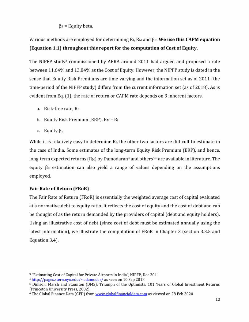
2.1. Airports’ Economic Regulatory Framework Worldwide
In order to understand the regulatory framework across the world, we studied 12 countries’
Regulatory Authorities regulating more than 25 airports. We documented the following:
• Till structure
• Methodology used to compute CoE
• Prescribed leverage
• Capitalization guidelines for airports
A detailed consolidation of the study is presented in Table R1. The following are the key
takeaways:
• Cost of Capital Methodology:
o None of the regulators mandate the use of CAPM as a method to estimate CoE
but most airports use it as a standard.
o Dublin (Ireland) uses a WACC methodology that incorporates additional
factors, like passenger pass-through time, baggage handling time, etc.
• Extent of Private Participation: Except for the United Kingdom and Australia in the
sample, governments hold more than 10% equity in their airports.
• Till Structure: Most airports apart from Singapore and Brazil follow a single or a dual
till mechanism. Singapore and Brazil follow a hybrid till.
• Leverage (D/E ratio): The regulators do not mandate or limit the operators to follow
a specific leverage. The 5-year actual leverage based on shareholders’ fund (SF) and
paid-up equity (PE) is discussed in Table R1.

17
o Changi Airport, wholly owned by the government, has the lowest leverage
using both SF and PE, i.e., 6.80% and 13.62%, respectively, across all the
international airports discussed here.
o Heathrow Airport has the highest leverage using both SF and PE, i.e., 83.41%
and 99.79%. This situation arose because nominal share capital was reduced
by a factor of 10 and transferred to distributable reserves, which were paid to
equity holders. This action resulted in lowering of equity and thereby
abnormally high leverages.
o Malaysia Airport Holdings Berhad (Holding Company) and Airports of
Thailand (Holding Company) use a debt and equity mix (SF 43.75% and PE
66.15%) that matches the average leverage across all the international
airports discussed here.
• Dividend Distribution: There is no mandate by any of the regulators to pay out
dividends.
o Malaysia Airport Holdings (MAHB) has made it a policy as a company to
declare 50% of its profits as dividends.
o Airports of Thailand have a policy of paying at least 25% of its profits as
dividends.
Given this understanding of the international regulatory scenario and capitalization
structure, we next move on to understand various international airports’ operation in terms
of their funding mechanism and returns they make for their private investors. For this
purpose, we first shortlist a set of international airports based on their proximity to BIAL in
these features. Next, we document the methodology used for shortlisting these airports.

18
Table R1: Regulatory Framework Worldwide
10 https://www.accc.gov.au/
11 https://comcom.govt.nz/ 12 https://www.caa.co.uk/home/
S. No.
Country
Col(1)
Regulating Authority
Col(2)
Norms for Till
Specified Col(3)
Calculation of COE specified(Yes/No) Col(4)
Book Debt to Shareholders’
Funds (Book Debt to Paid-Up Equity
Capital) 5-Year Avg.
Col(5)
Norm for Share Ownership Structure
Col(6)
1 Australia10
Australian Competition and Consumer Commission (ACCC)
Dual Till Not mandated, but uses CAPM, by way of Building Block Methodology.
• Sydney – 72.00% (49.48%) • Melbourne –
75.78% (95.96%)
• ACCC does not mandate. • The top 21 holders
(~91.20% holding) in Sydney do not include any of the government authorities.
2 New Zealand11
Commerce Commission (CC)
Dual Till
• Not Mandated • The CC takes an expert opinion from NERA
Economic Consulting (which uses CAPM) • CC computes WACC as per best available
estimates, defining a range. • The commission then compares it with post-
tax IRR, a combination of target returns for Aeronautical Pricing Activities and the forecast revenue of other regulated activities.
• CC checks whether the IRR falls within WACC range as computed earlier and makes a decision on WACC with the help of substantial supportive information.
• Auckland – 28.61% (81.33%)
• CC does not mandate. • But in Auckland, ~81.9%
of the total shares are publicly held and traded.
• Again ~18.1% of the shares are held by Auckland Municipal council
3 United
Kingdom12
Civil
Aviation
Authority
(CAA)
Single Till • Not Mandated
• However, CAA uses CAPM
• Heathrow – 83.41% (99.79%) • Gatwick – 80.14%
(82.79%)
• CAA does not mandate
19
Table R1: Regulatory Framework Worldwide
S. No.
Country Col(1)
Regulating Authority
Col(2)
Norms for Till
Specified Col(3)
Calculation of COE specified(Yes/No) Col(4)
Book Debt to Shareholders’ Funds (Book
Debt to Paid-Up Equity Capital)
5-Year Avg. Col(5)
Norm for Share Ownership Structure
Col(6)
4 South Africa13
No information available publicly
Single Till
• Airport charges are regulated through the use of a price cap formula13
• CPI-X, which limits the increase in a basket of revenue weighted tariffs to a rate of inflation (efficiency factor – X)
• The X-factor is determined by applying the building blocks methodology whereby each block of activities is identified, namely operating costs, depreciation, return on capital and taxation.
Data Not Available
No mandated norm but South African government owns 74.6%
5 South Korea No information available publicly.
6 Malaysia14
Malaysian Aviation Commission (MAVCOM - Primary Economic Regulator)
Single Till • Not Mandated • MAVCOM uses CAPM to estimate cost of equity.
Malaysia Airport Holdings Berhad (MAHB) – 43.75% (74.46%)
Malaysia Airports owns several airports across Malaysia. Retail shareholders hold~53.7% in MAHB.
7 Ireland15
Commission for Aviation Regulation (CAR)
Single Till • Not mandated • Uses CAPM to compute WACC with additional
factors like load, baggage handling time, etc.15
Dublin Airport Authority PLC – 48.26% (84.75%)
State ownership
8 Indonesia No information available publicly.
13 http://www.airports.co.za/business/investor-relations/economic-regulation 14 https://www.mavcom.my/en/home/ 15 http://www.aviationreg.ie/_fileupload/2014final/2014%20Final%20Determination.pdf

20
Table R1: Regulatory Framework Worldwide
S. No.
Country Col(1)
Regulating Authority
Col(2)
Norms for Till
Specified Col(3)
Calculation of COE specified(Yes/No) Col(4)
Book Debt to Shareholders’ Funds (Book Debt to Paid-
Up Equity Capital)
5-Year Avg. Col(5)
Norm for Share Ownership Structure
Col(6)
9 Singapore16 Civil Aviation Authority of Singapore
Hybrid Till (70–80%)16
CoE is computed as a sum of: • Computed pre-tax weighted average cost of capital
(WACC) on the average regulated asset base. • Computed pre-tax WACC on the average security
asset base not recovered
Changi Airport Group – 6.80% (13.62%)
Fully government owned
10 Netherland17
Human Environment and Transport Inspectorate
Dual Till Mandates use of WACC based on CAPM Schipol Group – 34.52% (95.98%)
PPP
12 Thailand18 Civil Aviation Authority of Thailand
Dual Till Not mandated but uses CAPM
Airports of Thailand – 20.90% (66.15%)
70% mandatorily government owned
13 Brazil19
National Civil Aviation Agency (ANAC)
Hybrid Till
• Not Mandated • ANAC uses CAPM to estimate cost of equity.
Data Not Available
PPP up to 60% observed
16 https://www.caas.gov.sg/ 17 https://english.ilent.nl/ 18 https://www.caat.or.th/en/ 19 http://www.anac.gov.br/en

21
2.2. Comparable Airports (Comparable to BIAL)
The above table (Table R1) provides information on airports in different jurisdictions and
assesses the existence of airport data). Europe, South Africa, South East Asia, and
Australasian regions were deemed to be relevant for the study. Middle East (hub airports)
and China (lack of credible data), the Americas (different environment) were excluded. Next,
within the four regions, the study narrowed down on 12 airports: Sydney, Melbourne,
Auckland, MAHB, AoT, Changi, Incheon, Heathrow, Gatwick, Dublin, Amsterdam, and
Johannesburg. Although Table R1 provides information on Brazil, we excluded it because it
lies in the Americas (different environment). Then, we assessed the (proximity score) of each
international airport to BIAL based on the following parameters.
• Revenue till structure:
o 1 – Single Till or where information is not available
o 2 – Dual Till
o 3 – Hybrid Till
• Ownership structure:
o 1 – if 100% Government Owned/Funded
o 2 – if Government / private owned/funded, not being Public Private
Partnership
o 3 – if Public Private Partnership Funded
• Operations Scale (OpS): For each comparable airport, k, we computed the ratios of
passenger, cargo, and aircraft movement of these airports to that of BIAL in each of
the years from 2015 to 2017. Note that all comparable airports are international
airports. These ratios are based on past 3 years’ data as available from the respective
airports’ websites/annual reports. Next, an equal weighted sum for these airports is
computed using average of the ratios under each category (passenger, cargo and air
traffic) as per Equation 2.120:
20 By construction, the OpS score for BIAL with respect to BIAL (itself) would be 3. To see this, note that each of
the ratios (RPi, RCi, RAi, for passenger, cargo and air traffic, respectively) for a given year would be equal to 1 by definition, and therefore an equally weighted average of these ratios must be equal to 1. Then, cumulating these numbers over the 3 years (2015 to 2017) would yield an OpS score of 3. If the OpS score for an international

22
𝑶𝒑𝑺𝒌 = ∑ (𝟏
𝟑) ∗ 𝑹𝑷𝒊 + (
𝟏
𝟑) ∗ 𝑹𝑪𝒊 + (
𝟏
𝟑) ∗ 𝑹𝑨𝑖
𝑖 =𝟐𝟎𝟏𝟕
𝑖 =𝟐𝟎𝟏𝟓
Equation 2.1 – Operations Scale
where OpSk = Operations scale for comparable airport k
i = Year 2015, 2016 and 2017
RPi = Ratio of passengers of the comparable airport to that of Bangalore airport,
Equation 2.2,
𝑹𝑷𝒊 =𝑷𝒊
𝑷𝑩
Equation 2.2 – Passenger Ratio
Pi = No. of passengers for the comparable international airport in year i
PB = No. of passengers for BIAL in year i
RAi = Ratio of aircraft movements of the comparable airport to that of Bangalore airport,
Equation 2.3 – Air Traffic Ratio,
𝑹𝑨𝑖 =𝑨𝒊
𝑨𝑩
Equation 2.3 – Air Traffic Ratio
Ai = No. of aircraft movements for a comparable international airport in year i
AB = No. of aircraft movements for BIAL in year i
RCi = Ratio of cargo of the comparable airport to that of Bangalore airport, Equation 2.4,
𝑹𝑪𝒊 =𝑪𝒊
𝑪𝑩
Equation 2.4 – Cargo Ratio
airport from the comparable set with respect to BIAL is 6, then we can conclude that the international airport’s scale of operation is about twice (score of 6 divided by 3) of that of BIAL.

23
Ci = Total cargo movement in metric tonne for a comparable international airport in year i
CB = Total cargo movement in metric tonne for BIAL in year i
• Finally, the proximity score for comparable airport, k, with respect to Bangalore airport
(B) is denoted by PSk,B. It is the net Euclidean Distance from each of the parameters w.r.t.
BIAL (Equation 2.5)
𝑷𝑺𝑘,𝐵 = √(𝑹𝑻𝑩 − 𝑹𝑻𝑘)𝟐 + (𝑶𝑺𝑩 − 𝑶𝑺𝑘)𝟐 + (𝑶𝒑𝑺𝑩 − 𝑶𝒑𝑺𝑘)𝟐
Equation 2.5 – Proximity Score w.r.t. BIAL
RTB = Revenue Till Score of BIAL
RTk = Revenue Till Score of comparable airport, k
OSB = Ownership structure Score of BIAL
OSk = Ownership structure Score of comparable airport, k
OpSB = Equal Weighted Operations Scale of BIAL
OpSk = Equal Weighted Operations Scale of comparable airport, k
Table 2.1 reports the scores of all airports considered with their weights w.r.t. BIAL. As
observed, Incheon Airport is out of bounds w.r.t BIAL. We discard this in the final analysis.
Intuition of the Proximity Score
The Proximity Score provides a Euclidean distance measure of a benchmark airport (from the comparable set) relative to the airport under consideration (BIAL, in this case). The proximity score considers three dimensions of comparison: (i) till mechanism, (ii) ownership structure, and (iii) operational scale. By construction, the proximity score for BIAL would be 0, but the proximity score of the benchmark international airport in the comparable set would depend on how different it is with respect to BIAL, with a high score indicating a dissimilar airport and a low score indicating a more similar airport.

24
Table 2.1: Proximity scores of different airports w.r.t BIAL
The table represents the difference between the scores for BIAL and the respective airport. The proximity score
is defined as 𝐏𝐒k,B = √(𝐑𝐓𝐁 − 𝐑𝐓k)𝟐 + (𝐎𝐒𝐁 − 𝐎𝐒k)𝟐 + (𝐎𝐩𝐒𝐁 − 𝐎𝐩𝐒k)𝟐, where RT stands for revenue till, OS
is Ownership and Funding Mechanism, and OpS is Operations. The subscripts B and k represent Bangalore and
the comparable airport, respectively. MAHB is the holding company of Kuala Lumpur Airport. AoT is the
holding company of Bangkok Airport.
S. No.
Airport
(Col 1)
Revenue Till
(RTB - RTk)
(Col 2)
Ownership Structure
(OSB - OSk)
(Col 3)
Operations
(OpSB - OpSk)
(Col 4)
Proximity Scores
(PSk,B)
(Col 5)
Bangalore 0.00 0.00 0.00 0.0000
1 Auckland 1.00 1.00 0.62 1.5449
2 Melbourne 1.00 1.00 -0.89 1.6716
3 Johannesburg 2.00 1.00 -0.04 2.2364
4 Gatwick 2.00 1.00 -0.94 2.4245
5 Sydney 1.00 1.00 -2.32 2.7171
6 Dublin 2.00 2.00 0.17 2.8333
7 Amsterdam 1.00 1.00 -8.34 8.4582
8 Changi 0.00 2.00 -8.34 8.5737
9 Heathrow 2.00 1.00 -8.75 9.0281
10 MAHB 2.00 1.00 -9.87 10.1161
11 Incheon 2.00 2.00 -10.36 10.7347
12 AoT 1.00 1.00 -11.83 11.9111

25
We have excluded the US and Canadian airports as their administrative, operations and
governance structure are significantly different from this set. Also, there is negligible
government participation in these airports. The Brazilian airports are relatively new to the
concept of privatization (~2011). Hence, we did not include airports from Brazil also.
We shortlisted 7 airports for a detailed study based on the overall proximity scores of these
airports. The criterion for the shortlist was governed by the proximity score, data
availability, and to ensure that we have a healthy mix of similarity and dissimilarity to
compare as well as contrast. Fig 2.1 map these airports w.r.t. BIAL on a radar chart based on
their proximity scores. The radar chart sweeps in the clockwise direction, with the proximity
score spiraling outwards. The scores range from ~1.5449 for Auckland to ~11.9111 for AoT.
The lower the score, the nearer the airport is w.r.t. BIAL.
We adhered to three principles in determining the comparison set of international airports:
(i) listed airports that provided market-based price data are preferred to unlisted airports,
(ii) if an airport is unlisted, we seek credible beta information from regulatory authority, if
available in public domain, and (iii) among comparison airports in the same
geography/jurisdiction, we give preference to the listed airports, and among the listed
airports, the one with more proximity.
Heathrow was excluded from the list to avoid geographical clustering (giving preference to
Gatwick because of its proximity to BIAL). In the case of Australia, regulators do not provide
any information on asset beta. The only recourse to a good estimate of beta is to rely on
market information . Since Sydney is a listed airport, we can estimate Sydney airport’s beta
using market data. Melbourne airport is unlisted, and the regulatory authority also does not
provide any estimate of beta. Thus, we prefer to include Sydney airport in our comparison
set despite Melbourne airport being more proximate to BIAL because Sydney airport’s beta
estimates can be reliably computed using market price data. Also, lack of comprehensive
data made us exclude Amsterdam airport, Incheon airport, and Johannesburg airport.

26
Fig 2.1: Airport Proximity Scores w.r.t. Bangalore
The chart depicts the scores of various parameters (Revenue Till, Ownership Structure, Operations and the Overall Proximity Score) of various international airports w.r.t. BIAL. All scores originate at BIAL (all scores are 0 here). As one sweeps clockwise, the Proximity Score moves away from Bangalore, thus making Auckland the nearest airport to Bangalore and AoT the farthest. Negative scores are possible only for Operations score. Heathrow airport was excluded to avoid geographical clustering (giving preference to Gatwick). The 6 airports (Sydney, Gatwick, Auckland, MAHB, AoT and Dublin) encircled in blue and 1 airport (Changi) encircled in red are used for comparative study vis-à-vis BIAL (sec 2.2). The airports encircled in blue (Sydney, Gatwick, Auckland, MAHB, AoT and Dublin) are used for asset beta computation of BIAL as discussed in chapter 3 (sec 3.2.1). MAHB is the holding company of Kuala Lumpur Airport. AoT is the holding company of Bangkok Airport.
Data Sources: Individual airports’ website; balance sheets and regulators’ website.
-15.00
-10.00
-5.00
0.00
5.00
10.00
15.00
Bangalore
Auckland
Melbourne
Johannesburg
Gatwick
Sydney
DublinAmsterdam
Changi
Heathrow
MAHB
Incheon
AoT
Airport Scores wrt Bangalore
Revenue Till Ownership & Funding Mechanism Operations Scale Proximity Score

27
We next analyze these airports vis-à-vis BIAL for its capitalization structure, funding
mechanism and investors’ returns.
2.2.1. Capitalization and Ownership Structure
Heathrow is 100% privately owned by Heathrow Airport Holdings Limited with no
government stake. The erstwhile government entity of British Airports Authority (BAA) was
privatized in 1987 and raised capital through the open market. It also constituted a part of
FTSE 100 with peak operating profits of GBP 11 million in the mid-1990s. It was delisted in
Recommendations (Comparable Set of International Airports for BIAL)
• The study considered different jurisdictions and assessed the existence of airport data and the relevance of the airport (See Table R1 of the study). Europe, South Africa, South East Asia, and Australasian regions were deemed to be relevant for the study. Middle East (hub airports) and China (lack of credible data), the Americas (different environment) were excluded. Next, within the four regions, the study narrowed down on 12 airports: Sydney, Melbourne, Auckland, MAHB, AoT, Changi, Incheon, Heathrow, Gatwick, Dublin, Amsterdam, and Johannesburg. These airports were considered for determining the proximity score because traffic density data was available.
• For estimating the asset beta (Chapter 3), we adhered to three principles in determining the comparison set of international airports: (i) listed airports were preferred to unlisted airports, (ii) if the airport is unlisted, we sought credible beta information from the regulatory authority, if available in public domain, and (iii) among comparison airports in the same geography/jurisdiction, we gave preference to the listed airports, and within the listed airports, the one with more proximity.
• The final comparison set for estimating asset beta consists of 6 airports (2 from Australasia – Sydney and Auckland, 2 from South East Asia – MAHB and AoT, and 2 from Europe - Gatwick, and Dublin). These airports were finally considered based on availability of market price data and the experience of the regulatory authority in assessing airport beta. The geographic spread of comparison set airports gives us confidence that the estimation of asset beta is robust.
• In the set of 6 airports considered for estimating asset beta, 4 airports are from developed countries and 2 airports from developing countries. Note that Indian airports face less demand risk because of generous true-ups offered in the PPP agreement. Thus, Indian airports are unlikely to face more systematic risk than developed country airports and can be benchmarked against comparable developed country airports in the comparison set.
• In the case of Australia, regulators do not provide any information on asset beta. Therefore, including a listed airport (Sydney) is preferable to including Melbourne because beta estimates can be reliably computed using market price data.
28
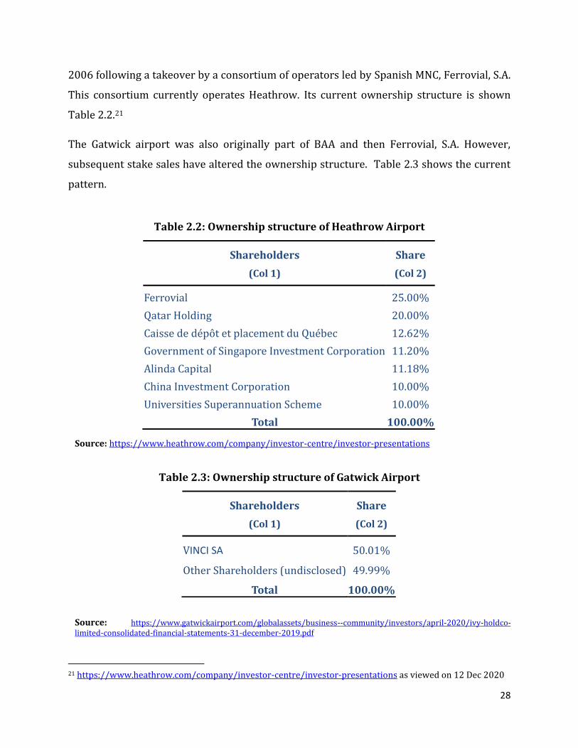
2006 following a takeover by a consortium of operators led by Spanish MNC, Ferrovial, S.A.
This consortium currently operates Heathrow. Its current ownership structure is shown
Table 2.2.21
The Gatwick airport was also originally part of BAA and then Ferrovial, S.A. However,
subsequent stake sales have altered the ownership structure. Table 2.3 shows the current
pattern.
Table 2.2: Ownership structure of Heathrow Airport
Source: https://www.heathrow.com/company/investor-centre/investor-presentations
Table 2.3: Ownership structure of Gatwick Airport Source: https://www.gatwickairport.com/globalassets/business--community/investors/april-2020/ivy-holdco-limited-consolidated-financial-statements-31-december-2019.pdf
21 https://www.heathrow.com/company/investor-centre/investor-presentations as viewed on 12 Dec 2020
Shareholders
(Col 1)
Share
(Col 2)
Ferrovial 25.00%
Qatar Holding 20.00%
Caisse de de po t et placement du Que bec 12.62%
Government of Singapore Investment Corporation 11.20%
Alinda Capital 11.18%
China Investment Corporation 10.00%
Universities Superannuation Scheme 10.00%
Total 100.00%
Shareholders
(Col 1)
Share
(Col 2)
VINCI SA 50.01%
Other Shareholders (undisclosed) 49.99%
Total 100.00%

29
Sydney and Auckland are publicly listed companies with the ownership structure as depicted
in Table 2.4 and Table 2.5, respectively.
Table 2.4: Ownership structure of Sydney Airport Source: https://assets.ctfassets.net/v228i5y5k0x4/4VyuoCbo3sqHVBggCxV7h3/5ad8f884f3ac89516391d8ea459d50ff/SYD_Annual_Report_2019_FINAL.pdf
Table 2.5: Ownership structure of Auckland Airport
Source: https://corporate.aucklandairport.co.nz/investors/results-and-reports
The two major international airports at Bangkok (Suvarnabhumi Airport and Don Mueang)
are owned and operated by a holding company, Airports of Thailand Public Company Limited
(AoT). This holding company is a government-owned publicly listed company.22 Totally,
70% of the ownership is held by the state’s Finance Ministry with foreign ownership capped
22 www.airportthai.co.th as viewed on 28 Feb 2020
Shareholders
(Col 1)
Share
(Col 2)
HSBC Custody Nominees (Australia) Limited 26.9%
BNP Paribas Nominees Pty Ltd 18.4%
J P Morgan Nominees Australia Limited 12.8%
Citicorp Nominees Pty Limited 6.6%
Balance Retail Holdings 35.3%
Total 100.00%
Shareholders
(Col 1)
Share
(Col 2)
Auckland Council Investments Limited 18.09%
Balance Retail Holdings 81.91%
Total 100.00%

30
at 30%, other major shareholders include Thai NVDR Company Limited (4.49%), South East
Asia UK (Type C) Nominees Limited (2.76%) and State Street Europe Limited (1.67%).
The Kuala Lumpur airport manages on very similar lines of Bangkok by Malaysia Airport
Holdings Berhad (MAHB), a holding company, in Table 2.6.
Table 2.6: Ownership structure of Malaysia Airport Holdings Berhad (MAHB)
Source: https://mahb.listedcompany.com/misc/ar/mahb_ar2019.pdf
The Changi airport and Dublin airport are fully state-owned airports, through subsidiary
companies.
Majority stake in BIAL is held by a consortium led by the FIH Mauritius Investments Ltd. The
shareholding patterns of the four (4) major Indian private airports (Bangalore, Delhi,
Mumbai, and Hyderabad) are provided in Table 2.7 through Table 2.10. The Indian
government (state/central or their subsidiary) has a 26% stake in each of these.
Shareholders
(Col 1)
Share
(Col 2)
Khazanah Nasional Berhad 33.21%
Citigroup Nominees (Tempatan) Son Berhad
(Employees Provident Fund Board) 13.06%
Balance Retail Holdings 53.73%
Total 100.00%

31
Table 2.7: Ownership structure of Bangalore International Airport Ltd. (BIAL)
Source: Website of BIAL23
Table 2.8: Ownership structure of Delhi International Airport Ltd. (DIAL)
Source: Annual Report of DIAL 2019-20
23 https://www.bengaluruairport.com/corporate/about-bial.html as viewed on 12 Dec 2020.
Shareholders
(Col 1)
Share
(Col 2)
Airport Authority of India 13.00%
Karnataka State Industrial and
Infrastructure Development Corporation Limited (KSIIDC) 13.00%
Siemens Project Ventures GmbH 20.00%
FIH Mauritius Investments Limited 54.00%
Total 100.00%
Shareholders
(Col 1)
Share
(Col 2)
Airport Authority of India 26.00%
GMR Airports Limited 64.00%
Fraport AG Frankfurt Airport Services Worldwide 10.00%
Total 100.00%

32
Table 2.9: Ownership structure of Mumbai International Airport Ltd. (MIAL)
Source: Business Standard, 1 Sep 202024
Table 2.10: Ownership structure of Hyderabad International Airport Ltd. (HIAL)
Source: Website of HIAL25
2.2.2. Funding Mechanism
As highlighted in Table 2.4 and Table 2.5, the Asset Management Companies (AMCs) and
pension funds are a major shareholder in Australia and New Zealand. In the case of Malaysia
and Thailand, the holding company is listed.
2.2.3. Trends in Airports Operations’
Fig 2.3 – Fig. 2.6 show the recent trends of passenger movement, total revenue, revenue/
passenger and Earnings After Tax (EAT) for all airports. As seen from these charts, all
parameters indicate a healthy state, with the following key takeaways:
24 https://www.business-standard.com/article/companies/adani-group-acquires-74-per-cent-stake-in-mumbai-international-airport-120083100215_1.html as viewed on 12 Dec 2020. 25 https://www.hyderabad.aero/our-company.aspx as viewed on 12 Dec 2020.
Shareholders
(Col 1)
Share
(Col 2)
Airport Authority of India 26.00%
Adani Group 74.00%
Total 100.00%
Shareholders
(Col 1)
Share
(Col 2)
Airport Authority of India 13.00%
Government of Telangana 13.00%
MAHB (Mauritius) Private Limited 11.00%
GMR Airports Limited 63.00%
Total 100.00%

33
• All airports have experienced a steady growth in passenger volumes (Fig 2.3) over
the period of 5 years.
• Revenue trends are also in sync with passenger trends (Fig 2.4) except for Delhi
(2017) and Hyderabad (2013).
• Earnings After Taxes (EAT) have also been rising except for Changi airport – Fig 2.6.
Fig 2.2: Passenger Movement Trends
Data Source: Passenger and traffic statistics published by the respective airports’ official website for international airports and the Airports’ Authority of India’s website for Indian airports.
-
10
20
30
40
50
60
70
80
90
100
2013 2014 2015 2016 2017
Pa
sse
ng
ers
in
Mil
lio
ns
Passenger Movement
Auckland Gatwick Dublin Sydney Changi
Bangkok Delhi Mumbai Bangalore Hyderabad

34
Fig 2.3: Revenue Trends
Data Source: Balance sheets of the respective airports
Fig 2.4: Revenue Per Passenger Trends
Data Source: Balance sheets and passenger movement data from official websites
0
500
1,000
1,500
2,000
2,500
2013 2014 2015 2016 2017
Re
ven
ue
in
Mil
lio
ns
US
DRevenues
Auckland Gatwick Dublin Sydney Changi
Bangkok Delhi Mumbai Bangalore Hyderabad
0
5
10
15
20
25
30
35
2013 2014 2015 2016 2017
Re
ven
ue
Pe
r P
ass
en
ge
r in
US
D
Revenue Per Passenger
Auckland Gatwick Dublin Sydney Changi
Bangkok Delhi Mumbai Bangalore Hyderabad

35
Fig 2.5: Earnings after Tax Trends
Data Source: Balance sheets of the respective airports
Given these insights, we now try to draw some lessons for the Indian airports. We tried to
establish a correlation between EAT vs. revenue per passenger. The hypothesis is, with an
increase in passenger movement and EAT, revenue per passenger should be fairly stable or
decrease. In other words, if traffic as well as EAT is healthy, the total airport charges per
passenger should be constant or decrease because being public services there is pressure on
airports to reduce tariffs whenever possible. Table 2.11 presents this scenario for our
comparable set of airports and Table 2.12 presents this scenario for Indian airports.
-100
0
100
200
300
400
500
600
700
800
2013 2014 2015 2016 2017
EA
T i
n M
Illi
on
s U
SD
Earnings After Tax
Auckland Gatwick Dublin Sydney Changi
Bangkok Delhi Mumbai Bangalore Hyderabad

36
Table 2.11 : Relationship between Revenue Per Passenger vs. EAT (Comparable Set)
[In this table, we try to test the following hypothesis: Does increase in passenger movement and EAT stabilize the Revenue per Passenger? This seems to be true for the comparables’ set.]
Airport
(Col 1)
EAT
Trend
(Col 2)
Passenger
Movement Trend
(Col 3)
Revenue Per Passenger Trend
(Col 4)
Correlation
Coeff.
(Col 5)
Auckland ↑ ↑ 0.9908
Sydney ↑ ↑ 0.7234
AoT* ↑ ↑ 0.1352
Singapore ↓ ↑ 0.3149
Gatwick ↑ ↑ 0.6333
Dublin ↑ ↑ 0.0857 Data Source: Balance sheets and official website of individual websites *Includes only passenger data, revenue data and earnings after tax data, for Bangkok and Don Mueang Airports only, not the holding company, Airports of Thailand as a whole.
Table 2.12: Relationship between Revenue per passenger vs. EAT (Indian Airports)
[In this table, we try to test the following hypothesis: Does increase in passenger movement and EAT stabilize the Revenue per Passenger? This seems to be true for the set of comparable airports (Table 2.11). It is not so for Indian airports.]
Airport
(Col 1)
EAT
Trend
(Col 2)
Passenger
Movement Trend
(Col 3)
Revenue Per
Passenger Trend
(Col 4)
Correlation
Coeff.
(Col 5)
Mumbai ↑ ↑ ↑ 0.1122
Delhi ↑ ↑ ↓ 0.7528
Hyderabad ↑ ↑ ↑ 0.6237
Bangalore ↑ ↑ ↑ 0.3218 Data Source: Balance sheets and AAI’s official website
As can be seen from Table 2.11, while EAT and revenues have been on an increasing
trajectory for Indian airports, revenue per passenger, on average, is marginally increasing
37
with positive and negative growths in individual years (except in the case of Delhi where it
has been decreasing consistently).
2.3. Associated Issues
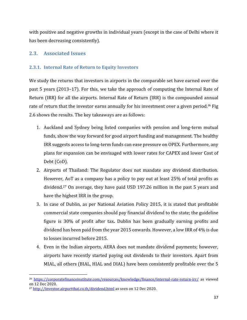
2.3.1. Internal Rate of Return to Equity Investors
We study the returns that investors in airports in the comparable set have earned over the
past 5 years (2013–17). For this, we take the approach of computing the Internal Rate of
Return (IRR) for all the airports. Internal Rate of Return (IRR) is the compounded annual
rate of return that the investor earns annually for his investment over a given period.26 Fig
2.6 shows the results. The key takeaways are as follows:
1. Auckland and Sydney being listed companies with pension and long-term mutual
funds, show the way forward for good airport funding and management. The healthy
IRR suggests access to long-term funds can ease pressure on OPEX. Furthermore, any
plans for expansion can be envisaged with lower rates for CAPEX and lower Cost of
Debt (CoD).
2. Airports of Thailand: The Regulator does not mandate any dividend distribution.
However, AoT as a company has a policy to pay out at least 25% of total profits as
dividend.27 On average, they have paid USD 197.26 million in the past 5 years and
have the highest IRR in the group.
3. In case of Dublin, as per National Aviation Policy 2015, it is stated that profitable
commercial state companies should pay financial dividend to the state; the guideline
figure is 30% of profit after tax. Dublin has been gradually earning profits and
dividend has been paid from the year 2015 onwards. However, a low IRR of 4% is due
to losses incurred before 2015.
4. Even in the Indian airports, AERA does not mandate dividend payments; however,
airports have recently started paying out dividends to their investors. Apart from
MIAL, all others (BIAL, HIAL and DIAL) have been consistently profitable over the 5
26 https://corporatefinanceinstitute.com/resources/knowledge/finance/internal-rate-return-irr/ as viewed on 12 Dec 2020. 27 http://investor.airportthai.co.th/dividend.html as seen on 12 Dec 2020.

38
years. However, BIAL and HIAL have recently started paying dividends, while DIAL
has paid dividends only once in 2017-18. MIAL is yet to declare dividends.
Fig 2.6: Past 5 years’ IRR based on Book and Equity Returns
Internal Rate of Return (IRR) is the compounded annual rate of return that the investor earns annually for his investment over a given period of time26. We computed the IRR based on book equity and their market capitalization (wherever applicable). The book equity method considers beginning equity, all dividends accrued (2013–2017) and ending equity (including retained earnings). The IRR based on market equity is the annualized market return based on market prices (including dividends for 2013–2017).
Data Source: Respective balance sheets of individual airports and Bloomberg for market data
2.3.2. Operators’ Returns: A Case of BIAL Divestment
In the FY 2009-2010, Bangalore Airport & Infrastructure Developers Private Limited
(BIADPL), a fully owned subsidiary of GVK Power & Infrastructure Limited, purchased a
stake of 43% from Flughafen Zurich AG, Switzerland and L&T Infrastructure Development
Projects Limited at a cost of INR 1,173.107 Crores. Again, during FY 2011-2012 BIADPL
infused a further capital of INR 613.820 Crores. However, for strategic reasons, they
offloaded 33% of their stake for a consideration of 2,202 Crores to Fairfax India Holdings
20%
13%
28%
18%
25%
10%7%
4%
34%
-6%
16%
47%
18%
-10%
0%
10%
20%
30%
40%
50%
IRR
IRR 2013-2017
IRR (Book Equity) IRR (Market Equity)

39
Corporation (FHC). Then, in FY 2017-18, they completed the exit by selling off their
remaining stake of 10% at 1,290 Crore. During their holding period, they also received a
dividend of INR 16.54 Crores in the year 2016-2017. The net profit turns out to be ~95% or
INR 1,783 Crores over 9 years. We performed an annual Internal Rate of Return (IRR)26
analysis to understand the real returns accrued to BIADPL. Table 2.13 details the working of
the same.
Table 2.13: IRR computation for BIAL divestment (All amounts in INR Crore)
2009-2010
2010-2011
2011-2012
2012-2013
2013-2014
2014-2015
2015-2016
2016-2017
2017-2018
Investments (1,173)
(614) 0 0 0 0 0 0
Dividend 0 0 0 0 0 0 0 166 0
Sale proceeds
0 0 0 0 0 0 0 2,2017 1,290
Cash flows for IRR
(1,173) 0 (614) 0 0 0 0 2,2183 1,290
IRR 10.57% Data Source: Balance Sheets of BIAL and GVK from 2009 – 2018
As observed from Table 2.13, the net IRR is 10.57% per annum for the given holding period
of 9 years from 2009–’18. This appears to be quite close to the AERA recommended return
for the second control period (FY2016-17 to FY2020-21), viz. ~11.33%, but lower than
BIAL’s submission of 17%.28
2.3.3. Prevalent Trends in other Infrastructure Space
Securities and Exchange Board of India (SEBI) framed guidelines to set up the Infrastructure
Investment Trust or InVITs like REITs. The structure of the same is showcased in Fig 2.7.
Essentially, these InVITs function as a mutual fund, enabling individual/institutional
investors to gain an exposure to the stable cash flows from an infrastructure asset without
being exposed to the risks involved in setting them up. As per the regulations, completed and
28 AERA Consultation Paper No. 05/ 2018-19 from file: AERA/20010/MYTP/BIAL/CP-II/2016-17/Vol-III

40
revenue generating projects in PPP mode are eligible to be securitized through this
procedure. Several projects in the roads and power sector are part of InVITs.
As of 2018, a prominent InVITs in the road space was IRB InVIT Fund sponsored and
managed by IDBI. This had an income of 5,157 Cr. with 13 road projects. Another prominent
InVIT in the power sector was IndiGrid sponsored and managed by the Sterlite group. This
had an income of 406 Cr with 6 project SPVs.
The InVIT structure could be considered as one of the options while privatizing other
airports owned by the Government of India.
Fig 2.7: Framework for InVITs,29
Source: Ernst & Young Report on Infrastructure Investment Trusts
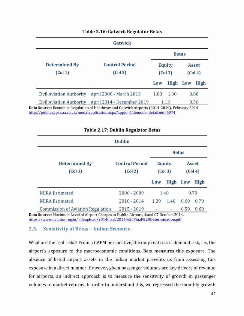
2.4. Determinants of CoE used in the Set of Comparable Airports
As we saw in section 2.1, although none of the regulators mandate the CAPM methodology,
all the airport operators use the CAPM to determine the Cost of Equity. We know that the
risk-free rate and ERPs in the CAPM equation (Equation 1.1) are macro-economic in nature,
but the key in CoE determination is the equity beta. Regulators of Auckland airport,
Heathrow airport, Gatwick airport and Dublin airport state the betas that they use in their
29 PM in figure refers to Project manager.

41
CoE computations. Table 2.14 – Table 2.17 show the asset and equity betas for different
control periods used in Heathrow, Gatwick, Dublin and Auckland across control periods.
Table 2.14: Auckland Regulator Betas
Auckland
Determined By
(Col 1)
Control Period
(Col 2)
Betas
Equity
(Col 3)
Asset
(Col 4)
Low High Low High
Commerce Commission July 2008 - June 2012 0.68 1.08 0.50 0.70
Commerce Commission July 2013 - June 2017 0.89 0.60
Commerce Commission July 2017 - June 2022 0.74 0.60 Data Source: Final Report - Auckland International Airport’s Pricing Decisions (July 2017 – June 2022), dated 01 November 2018, ISBN No. 978-1-869456-65-8 https://comcom.govt.nz/regulated-industries/airports/projects/review-of-price-setting-event-3#projecttab
Table 2.15: Heathrow Regulator Betas
Heathrow
Determined By
(Col 1)
Control Period
(Col 2)
Betas
Equity
(Col 3)
Asset
(Col 4)
Low High Low High
Civil Aviation Authority April 2008 - March 2013 0.90 1.15 0.56
Civil Aviation Authority April 2014 - December 2019 1.10 0.50
NERA Estimated January 2020 - December 2024 1.30 1.40 0.55 0.60 Data Source: Economic Regulation of Heathrow and Gatwick Airports (2014-2019), February 2014 http://publicapps.caa.co.uk/modalapplication.aspx?appid=11&mode=detail&id=6074
42
Table 2.16: Gatwick Regulator Betas
Gatwick
Determined By
(Col 1)
Control Period
(Col 2)
Betas
Equity
(Col 3)
Asset
(Col 4)
Low High Low High
Civil Aviation Authority April 2008 - March 2013 1.00 1.30 0.80
Civil Aviation Authority April 2014 - December 2019 1.13 0.56 Data Source: Economic Regulation of Heathrow and Gatwick Airports (2014-2019), February 2014 http://publicapps.caa.co.uk/modalapplication.aspx?appid=11&mode=detail&id=6074
Table 2.17: Dublin Regulator Betas
Dublin
Determined By
(Col 1)
Control Period
(Col 2)
Betas
Equity
(Col 3)
Asset
(Col 4)
Low High Low High
NERA Estimated 2006 - 2009 1.40 0.70
NERA Estimated 2010 - 2014 1.20 1.40 0.60 0.70
Commission of Aviation Regulation 2015 - 2019 - - 0.50 0.60 Data Source: Maximum Level of Airport Charges at Dublin Airport, dated 07 October 2014. https://www.aviationreg.ie/_fileupload/2014final/2014%20Final%20Determination.pdf
2.5. Sensitivity of Betas – Indian Scenario
What are the real risks? From a CAPM perspective, the only real risk is demand risk, i.e., the
airport’s exposure to the macroeconomic conditions. Beta measures this exposure. The
absence of listed airport assets in the Indian market prevents us from assessing this
exposure in a direct manner. However, given passenger volumes are key drivers of revenue
for airports, an indirect approach is to measure the sensitivity of growth in passenger
volumes to market returns. In order to understand this, we regressed the monthly growth

43
rate in passenger volumes for BIAL on the monthly returns for the Indian stock market. The
passenger growth rate can be viewed as a proxy for the demand driver for BIAL. The stock
market return captures the fluctuations in macroeconomic conditions. A high value of the
slope from this regression would indicate high exposure of BIAL to demand risk and vice-
versa. We found very low regression coefficients (~0.3), thus indicating that the demand for
BIAL is relatively inelastic and highly constrained by supply under normal circumstances.
Appendix 3 details the methodology and results of this analysis.
2.6. Conclusion
In this chapter, we saw the regulatory framework of various airport regulators across the
world with a focus on CoE. The key takeaways are as follows:
• All of them use CAPM as a method to estimate CoE but none mandate it.
o Only Dublin uses a complicated model based on operational metrics/ad hoc
assumptions.
• D/E ratios are not mandated, however, the actual D/E ratios using shareholders’ fund
and paid-up equity range from 43.75% to 81.33%.
Next, we identified airports that were closest to BIAL w.r.t. operations, ownership structure
and till. Then, we studied these comparable airports for any lessons for Indian airports in
general, and BIAL. A valuable lesson to be drawn is that CAPEX requirements can be
addressed through the open market route. Also, we concluded that while other airports are
in a mature or saturated phase, Indian airports are still in a growth phase with high potential.
Furthermore, this argument is strengthened by the demand analyses of Indian airports. Also,
we looked at other sectors like road and power and how InVITs is helping cash flows.
Given we have now identified our comparables’ set, we are all set to go ahead with CoE
estimation for BIAL. As we have established the distance of these airports, we evolve
methodologies to impute the betas for BIAL. The next chapter is devoted to establishing
these estimates and determining CoE and providing an illustrative example for FRoR
computation.

44
This page is intentionally left blank.

45
Chapter 3 – Determination of Cost of Equity and Fair Rate of Return
Airport regulators world over use the Capital Asset Pricing Model (CAPM) to estimate the
Cost of Equity (CoE) for their private operators. Further, these costs are estimated in blocks
of time period keeping in mind the current macro-economic realities as well as operational
requirements. This is true of AERA as well. It is done for 5 years “Control Periods”. The
current control period for BIAL ends on 31.03.2021 and the next 5 years’ control period is
from FY2021-22 to FY2025-26. In this chapter, we estimate the CoE and provide an
illustrative example of FRoR computation for BIAL. As highlighted in chapter 2, we identified
6 international airports that were very similar to BIAL in terms of their operations, funding
mechanism and till structures and studied them in detail. Further, we also highlighted the
pertinent lessons for Indian airport operators and regulators therein.
First, we revisit the CAPM methodology and state the assumptions and the relevance therein.
Next, we elaborate on the process of obtaining the individual components of CoE, viz., betas
(assets as well as equity), risk-free rate and the Equity Risk Premium (ERP). Finally, we
provide an illustrative example of the CoD and FRoR computation.
3.1. Capital Asset Pricing Model
The Capital Asset Pricing Model was developed in the 1960s by Sharpe30 (1964) and Lintner
(1965).31 It can be used to estimate a project’s cost of capital, which is the expected rate
demanded by potential investors. The cost of capital is used to assess the value of risky cash
flows from investment projects made by businesses. According to the CAPM, the project’s
cost of capital is linearly related to a measure of project risk (known as beta), which
essentially captures the sensitivity of the project’s cash flows to the state of the economy.
The greater is the sensitivity, the greater is the risk faced by potential investors and the
greater is the expected return of these investors, or the cost of capital. Thus, estimating the
30 Sharpe, William F. 1964. Capital asset prices: A theory of market equilibrium under conditions of risk. Journal of Finance 19 (September): 425–42. 31 Lintner, John. 1965. The valuation of risk assets and the selection of risky investments in stock portfolios and capital budgets. Review of Economics and Statistics 47 (February): 13–37.
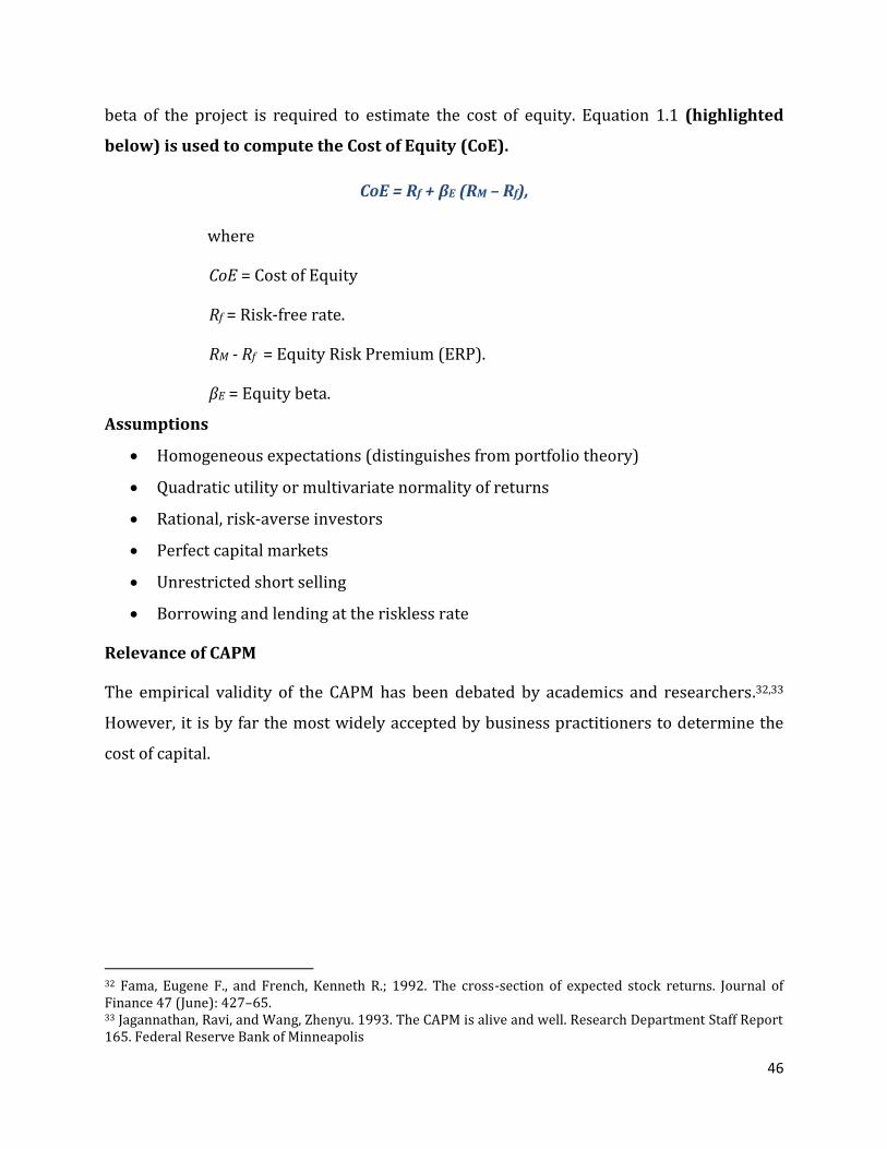
46
beta of the project is required to estimate the cost of equity. Equation 1.1 (highlighted
below) is used to compute the Cost of Equity (CoE).
CoE = Rf + βE (RM – Rf),
where
CoE = Cost of Equity
Rf = Risk-free rate.
RM - Rf = Equity Risk Premium (ERP).
βE = Equity beta.
Assumptions
• Homogeneous expectations (distinguishes from portfolio theory)
• Quadratic utility or multivariate normality of returns
• Rational, risk-averse investors
• Perfect capital markets
• Unrestricted short selling
• Borrowing and lending at the riskless rate
Relevance of CAPM
The empirical validity of the CAPM has been debated by academics and researchers.32,33
However, it is by far the most widely accepted by business practitioners to determine the
cost of capital.
32 Fama, Eugene F., and French, Kenneth R.; 1992. The cross-section of expected stock returns. Journal of Finance 47 (June): 427–65. 33 Jagannathan, Ravi, and Wang, Zhenyu. 1993. The CAPM is alive and well. Research Department Staff Report 165. Federal Reserve Bank of Minneapolis

47
Discussion Summary on Estimation Approach
• While the CAPM is a theoretical model based on assumptions that do not necessarily hold
in the real world, its simplicity and intuitive appeal have made it the on-going favorite
model for determining cost of equity in any market-based economy. Our procedures for
determining Cost of Equity using the Capital Asset Pricing Model are consistent with the
best practices adopted by international airport regulatory authorities and by regulatory
authorities across the world for a wide range of utilities (Table R1, Ch. 2).
• In particular, the CAPM says that the cost of equity should be related to demand (or
business) risk, as measured by correlation of a firm’s stock returns with the returns on
the market portfolio. More importantly, the CAPM points out that idiosyncratic difference
in firms should NOT affect the cost of equity because investors in a market-based economy
hold portfolios rather than individual assets and thus are able to diversify away the
idiosyncratic risk exposure. In short, idiosyncratic factors (e.g., airport specific factors)
do not affect the estimation of cost of equity when using the CAPM methodology.
• Furthermore, it is important to note that “true-up” of costs afforded to Indian airports
shields them from demand risk; this is a feature that indicates that Indian airport
operators (under the PPP arrangement) face low systematic risks and in that sense,
developed country airports can also be used as benchmarks while estimating asset beta.
• Given the conceptual underpinnings of CAPM (as pointed out above), the standard
approach is to find a comparable set of airports and impute a cost of equity based on the
betas for a comparable set of firms. Our approach accounts for ownership structure,
operational scale, revenue till arrangement while identifying the “optimal” mix of
comparable airports. Thus, comparable airports that are more proximate to BIAL are
given more weightage when averaging the asset betas of comparable airports to estimate
the asset beta of BIAL. This procedure essentially implies that the proximity-score
weighted average asset beta of comparable firms mimics a tracking portfolio of firms
that provides the best proxy for the systematic risk inherent in BIAL.
• In summary, we use a procedure that is consistent with the application of the CAPM and
which accounts for key differences in ownership, funding, and operation scale. Our
approach is also unique in that it is driven by actual data considerations rather than
plausible motivations for drivers of cost of equity.

48
3.2. Methodology for CoE Estimation
As seen in section 3.1, we need three components to estimate the CoE using CAPM. These
components are the risk-free rate (Rf), equity beta and the equity risk premium (ERP). Rf and
ERP are mostly macro-economic in nature and thus one can rely on time-series data to
estimate these variables. However, determining the equity beta is more challenging,
especially for unlisted companies such as BIAL. As will be discussed in section 3.2.1, we
overcome this issue by using a set of comparable airports. We use the Rf that is available
from public sources. For determining ERP, we combine our own estimates for ERP (study by
Anshuman, Biswas, Jain and Sharma, 2019) with the ERP estimates from Grant Thornton and
Damodaran.34 For the purpose of illustration, we estimate the cost of Debt (CoD) of BIAL by
determining the cost of debt for infrastructure firms that have issued debt with a similar
credit rating as BIAL.
The control periods for DIAL and MIAL are slightly staggered from that of BIAL and HIAL. To
maintain consistency in the cost of equity estimates across the four major PPP airports, we
have used the same time-period to estimate of ERP and risk-free rate for BIAL and HIAL as
used for DIAL and MIAL. This consistency in approach for the four major PPP based airports
is advisable given that there is transient variation in equity risk premium which can
differentially impact the cost of equity of these airports.35
3.2.1. Methodology Summary
Now that we have the set of comparable airports and computed their respective Proximity
Distance Scores w.r.t. BIAL (sec 2.2), we can now move on to estimating the Cost of Equity
(CoE) and providing an illustrative example of Fair Rate of Return (FRoR) computation.
Here are the steps involved in the process:
1. Unlever the betas of listed Comparable Airports (secs 3.2.32 and 3.3.2)
34 Anshuman, Biswas, Jain, and Sharma (2019); Predictability of Equity Risk Premium in India. 35 For instance, the market fell by around 30% in the first three months and then recovered the entire loss by the end of the year. These large fluctuations are unprecedented and related to the Covid crisis. ERP estimates fluctuate between 5.2% to 7.2% over 2020 depending on time at which it is estimated.

49
2. Next, we estimate Asset Betas for BIAL (secs 3.2.3 and 3.3.3) with Proximity
Distance Scores (sec 2.2) as inputs
3. Then, we re-lever Asset Betas to get Equity Betas for BIAL (secs 3.2.4, 3.3.4 and
3.3.4) with Target Gearing Ratios (sec 3.3.4) as inputs
4. Next, we obtain the CoE (sec 3.3.9) using Equity Risk Premium or ERP (sec 3.3.6)
and Risk Free Rate (sec 3.3.9) as inputs
5. Finally, we illustrate the computation of the FRoR (sec 3.3.9) with Cost of Debt
(CoD) as an input (sec 3.3.7). Please note that this computation is for illustrative
purpose only as CoD is time sensitive. The CoD must be estimated based on
information available at that point in time in future. The entire process is
summarized as a flowsheet in Appendix 4.
3.2.2. Un-levering the Betas of the Listed firms in the Comparable Airports’ Set
The comparable set consists of 6 airports – viz. Auckland, Airports of Thailand (AoT), Dublin,
Gatwick, Malaysia Airports Holdings Berhad (MAHB) and Sydney. For AoT, MAHB and
Sydney, which are listed airports, we can compute equity betas based on market data. We
use the following methodology to estimate the asset betas from the equity betas:
• Estimate the equity betas for listed airports from our comparables’ set through a
regression of returns of these stocks on the returns of the relevant market index using
data from Bloomberg.
• Un-lever these equity betas to find the corresponding asset betas using Equation 3.1.
𝜷𝑨 =𝜷𝑬
[𝟏 + (𝟏 − 𝑻𝑪) ∗𝑫𝑬]
Equation 3.1 – Unlevering Betas
where
ßA = Asset Beta,
ßE = Equity Beta,
TC = Marginal Tax Rate,
D/E = Actual Market Debt to Equity Ratio

50
Dublin and Gatwick airports are unlisted but have estimates for asset betas from their
respective regulators. Auckland airport is a listed airport, and its beta can be estimated from
market data, but the New Zealand regulatory authority has assigned a specific value for the
Auckland Airport asset beta after extensively analyzing market data and other airport-
specific information. In this case, we give preference to the regulator assigned asset beta
because it is based on a comprehensive study.
3.2.3. Estimating Asset Betas for BIAL
Next, we estimate the asset betas for BIAL by two (2) different methods, viz.:
1. Equal weighted average of these 6 airports’ asset betas
2. Weighted average of these 6 airports’ asset betas. The weights are the inverse
proximity score from BIAL using Equation 3.2.
𝜷𝐴 =
∑ (𝜷𝑘
𝑃𝑆𝑘,𝐵 )𝟔
𝑘=𝟏
∑ (𝟏
𝑃𝑆𝑘,𝐵)𝟔
𝑘=𝟏
Equation 3.2 – Weighted Avg. Betas
where
ßA = Unlevered Asset betas for BIAL
ßk = Unlevered asset betas for comparable airports, k, viz. MAHB, Sydney, AoT and
Regulator estimated Asset Betas, for Auckland, Gatwick, and Dublin airports.
𝑃𝑆𝑘,𝐵 is the proximity score of the comparable airport, k, with respect to BIAL.
The proximity score weighted (PSW) betas represents a more refined estimate of the true
asset betas in contrast to the equally weighted counterpart as it incorporates the degree of
similarity between BIAL and the airports in the comparable set.
3.2.4. Re-levering the BIAL’s Asset Beta to get Equity Beta
We estimate equity beta for BIAL by re-levering the asset beta assuming a Target market
Debt to Equity (D/E) ratios using Equation 3.3.

51
𝜷𝑬 = 𝜷𝑨 ∗ [𝟏 + (𝟏 − 𝑻𝑪) ∗𝑫
𝑬]
Equation 3.3 – Re-levering Betas
where
ßA = Asset Beta,
ßE = Equity Beta,
TC = Marginal Tax Rate,
D/E = Target Market Debt to Equity Ratio
3.2.5. Cost of Equity and FRoR
With all components of CoE now available, we can compute the CoE using the CAPM
equation. Once we have CoE, we can also compute FRoR using the Equation 3.4.
𝑭𝑹𝒐𝑹 = (𝑹𝑫 ∗ 𝒈) + 𝑹𝑬 ∗ (𝟏 − 𝒈)
Equation 3.4 – Fair Rate of Return
where
g = Target Debt to (Debt + Equity) Ratio
RD = Cost of Debt
RE = Post-Tax Cost of Equity
Apart from CoE, the Cost of Debt (CoD) is the key components of Equation 3.4. The Cost of
Debt (CoD) is estimated as the coupon rate for bonds issued with similar credit ratings as
BIAL.
The entire process flow with relevant sections numbers is showcased in Appendix 4.

52
3.3. Results and Discussion
Below, we present all the relevant results leading up to the computation of CoE and FRoR.
We start with shortlisting of airports for beta computations followed by asset and equity
betas for them. This is followed by a section on Cost of Debt and finally the CoE and FRoR.
3.3.1. Shortlisting Relevant Airports for Asset Betas for BIAL
The comparable set consists of six international airports. Of these, three airports, Sydney,
MAHB and AoT are listed companies with traded stocks. Listed airports are chosen to ensure
that their equity betas are readily available for computation using price data from a
commercial source like Bloomberg. The asset betas for these airports are computed from the
estimated equity betas. For the other three airports, Auckland, Gatwick and Dublin, the
country regulatory authorities have provided direct estimates of asset betas for the
forthcoming control periods.
3.3.2. Results Related to Estimating Asset Betas of Airports in the Comparable Set
We estimate the asset betas for 6 airports (AoT, Auckland, Dublin, Gatwick, MAHB and
Sydney) from the comparable set. For three of these airports (AoT, MAHB and Sydney), we
use price date to estimate their equity betas and adjust for leverage to calculate their asset
betas. For the other three airports (Auckland, Dublin, and Gatwick), we rely on the estimates
of asset beta provided by the relevant regulatory authorities. Table 3.1 shows the equity and
asset betas of AoT, MAHB and Sydney. The equity betas are obtained from Bloomberg and
corresponding asset betas are estimated by un-levering using Equation 3.1. As highlighted,
the asset betas range from 0.40 for Sydney to 0.86 for AoT. Table 3.1 shows the regulator
estimated asset betas of Auckland, Dublin, and Gatwick. As highlighted, the asset betas range
from 0.55 for Dublin to 0.60 for Auckland.

53
Table 3.1: Asset and Equity Betas for 3 Comparable International Airports
Note: The equity betas are directly sourced from Bloomberg. The asset betas are computed as βA=βE/[1+(1-TC)*D/E] (Equation 3.1). *** Indicates a 99% statistical significance level of beta estimate.
Airport
(Col 1)
Equity
Beta36
(Col 2)
Marginal Tax Rates37
(Col 3)
3-Year Avg. Market Debt Equity
(Col 4)
Asset
Beta38
(Col 5)
Sydney 0.5641*** 30.00% 0.5859 0.4000
MAHB 1.0573*** 24.00% 0.4927 0.7693
AoT 0.8895*** 20.00% 0.0456 0.8582
Data Sources: Bloomberg for Equity Betas; Deloitte Inc. for marginal tax rates
Table 3.2: Regulator Estimated Asset Betas for 3 Comparable International Airports
Airport
(Col 1)
Regulator
Asset Beta
(Col 2)
Reference
(Col 3)
Auckland 0.60 Table 2.14
Dublin 0.55* Table 2.17
Gatwick 0.56 Table 2.16 *The regulatory authority has provided two estimates: a low asset beta and a high asset beta. We use the simple average of the low asset beta (0.50) and the high asset betas (0.60), i.e., 0.55.
3.3.3. Results Related to Estimation of Asset Betas for BIAL
Using the methodology described in section 3.2.1, we first computed the asset betas for BIAL
using two different techniques, viz. equally weighted and proximity score weighted
(Equation 3.2). As discussed earlier as well, the proximity score weighted (PSW) beta better
represents the true asset beta as compared to the equally weighted counterpart as they
account for the similarity between the Indian airport and the airport in the comparables’ set.
36 Source: Bloomberg data from 2016 – 2018 weekly returns 37 https://www2.deloitte.com/global/en/pages/tax/articles/global-tax-rates.html, as viewed on 28 Feb 2020 38 βA=βE/[1+(1 – TC)*D/E] – Equation 3.1

54
Table 3.3: Asset Betas for BIAL.
Equally weighted is simple average of comparables’ asset betas. PSW is the weighted average of the asset betas
with the weights being the (inverse) Proximity Score of the airport (Equation 3.2).39 The proximity score weighted (PSW) beta is a more refined estimate that accounts for airport-specific information.
Equally Weighted
Average Asset Beta Proximity Score Weighted
Average Asset Beta
BIAL 0.6229 0.564689
3.3.4. Re-levering Asset Betas of BIAL
Re-levering the asset betas to estimate the equity betas for BIAL is done by assuming a target
gearing ratio using Equation 3.3. In Table 3.4, one can see the gearing ratios employed by
different international airports for computing the weighted average cost of capital (WACC)
in column (2). The column (3) shows the average 5-year book debt to equity ratio (based on
paid-up equity capital, as has been done in the case of BIAL). It is evident that the gearing
39 βA = ∑ (
𝛃kPSk,B
)𝟔k=𝟏
∑ (𝟏
PSk,B)𝟔
k=𝟏
(Equation 3.2 – Weighted Avg. Betas)
Recommendation (Proxy for Asset Beta of BIAL)
• We discussed the two different ways to compute proxies for assets betas of BIAL. Our
recommendation based on the proximity score weighted beta estimate is more reliable. The equally weighted approach is useful only when the comparable set of airports is picked from the same environment.
• Statistically speaking, if the sample consists of observations from different distributions with different population means, taking a simple statistic like the sample average will be biased. In such cases, a weighted average rather than a simple average in which the weights recognize the degree of difference between the sample observation and the relevant population distribution is considered. Our proximity score weighted beta approach accounts for the “closeness” of the comparable airports to BIAL.
• The recommended asset betas for BIAL is 0.564689

55
ratio is significantly lower than the book debt to equity ratio for all international airports.40
The average gearing ratio is 48% but the 5-year average of the book debt to equity ratio is
83%. Further, we plotted the best-fit linear trend between these two variables, as shown in
the chart below. We can see that R-square is virtually 0 suggesting that the two variables are
unrelated. Furthermore, both the economic and statistical relation between the two
variables is negligible. The coefficient is virtually 0 and the t-stats are also insignificant.
40 We were able to use a larger comparable set of international airports – this gives us more confidence in the estimates.

56
Table 3.4: Target Gearing Ratios
Airport
(Col 1)
Target Gearing
Ratio
(Col 2)
5-Year Avg. BDE based on Paid-
Up Equity (based on Share
Holder Fund)
(Col 3)
Citation
(Col 4)
Source
(Col 5)
Auckland 19.00% 81.33%
(28.61%)
Review of Auckland International Airport’s pricing decisions and expected performance (July 2017 – June 2022), November 2018, Pg. 97, Table A1.
https://comcom.govt.nz/regulated-industries/airports/projects/review-of-price-setting-event-3#projecttab
Heathrow 60.00% 99.79%
(83.41%) UKRN, Cost of Capital – Annual Update Report, June 2018, Pg. 11, Table
https://www.ukrn.org.uk/wp-content/uploads/2018/11/2018-UKRN-Annual-WACC-Summary-Update-v2.pdf
Gatwick 55.00% 82.79%
(80.14%) UKRN, Cost of Capital – Annual Update Report, June 2018, Pg. 11, Table
https://www.ukrn.org.uk/wp-content/uploads/2018/11/2018-UKRN-Annual-WACC-Summary-Update-v2.pdf
Sydney 55.00% 49.48%
(72.00%) Pricing Proposal 2016-2021, Pg. 16, Table 9
http://www.airservicesaustralia.com
Melbourne 55.00% 95.96%
(75.78%) Pricing Proposal 2016-2021, Pg. 16, Table 9
http://www.airservicesaustralia.com
Dublin 50.00% 84.75%
(48.26%)
Commission for Aviation Regulation, Maximum Level of Airport Charges at Dublin Airport 2014 Determination, Pg. 90, Para 7.118.
https://www.aviationreg.ie/regulation-of-airport-charges-dublin-airport/2019-determination.841.html
MAHB 50.00% 74.46%
(43.75%)
MAVCOM Aeronautical Charges Framework, October 2018, Pg. 26, Table 9. (Is 40-60%, but a mid-point average of the two taken)
https://www.mavcom.my/wp-content/uploads/2018/10/181019_Aeronautical-Charges-Framework-Consultation-Paper-Final-1.pdf
Amsterdam 40.00% 95.98%
(34.52%)
Amsterdam Airport Schiphol Operation Decree, 2017, WACC - Part C of Appendix to Article 32, Pg. 19.
https://www.schiphol.nl/en/download/b2b/.../1T8kLVjBBmOiaKqOO4WC0K.pdf
Average 48.00% 83.07%
(58.31%)

57
Fig 3.1: Regression Results for Market D/E (MDE) vs. Book D/E (BDE) for Listed International Airports
From the data in Table 3.4, we regress the Target Gearing Ratio for the comparable set as a function of their Actual 5-Year Average Book D/E (2013 – 17) period.
There is a good reason to use a lower target gearing ratio rather than the gearing ratio
suggested by the debt to book-equity values. First, the WACC should reflect a long-term
steady state gearing ratio which may not be reflected in the current gearing ratio. Second,
the WACC is supposed to be determined using market value weights for debt and equity.
Since equity values tend to rise over time, it is typically the case that market value based debt
to equity ratios will be much lower than book debt to equity measures. While the airports do
not explicitly mention this factor as a reason for using lower target gearing ratios than that
suggested by book ratios, we believe that this factor could be a significant reason.
To get additional confirmation, we consider the four airports for which we have listed equity
securities and estimate the 5-year average of the market debt to equity ratio. The 5-year
average leverage using market capitalization (MDE) for the comparable set of listed airports
(AoT, Auckland, MAHB and Sydney) is equal to 0.3503 (D/E) or 25.94% (D/D+E). These
y = -0.0071x + 0.4859R² = 8E-05
0%
10%
20%
30%
40%
50%
60%
70%
0% 20% 40% 60% 80% 100% 120%
Ta
rge
t G
ea
rin
g R
ati
o
5-Year Avg. BDE Using Paid-Up Equity
Comparable Airports LeverageTarget Vs. Actual

58
figures are also much lower than book debt to equity ratios. Given these findings, we can be
reasonably assured that the low gearing ratio of the international airports is consistent with
the idea that market-based debt to equity ratios should be used in computing the cost of
capital.
As an additional benchmarking exercise, we also estimated the relation between the market
debt to equity and the book debt to equity ratio of a typical infrastructure firm in India. To
estimate the relation between market debt to equity ratio and book debt to equity ratio, we
first regressed MDE on BDE for various infrastructure companies, using price data for 37
listed infrastructure companies over the recent 5 years. In other words, we estimated the
following empirical relation between the two variables, under the restriction that the
intercept is 0.
MDE = f * BDE
Equation 3.5 – BDE/ MDE Relation
where f is the regression coefficient.
The total valid data points in the clean sample were 121. The filters used to remove outliers
in the data were an upper cap of 5 for BDE (equivalent of BDE 83:17) and a lower bound of
0 (no debt). Table 3.5 shows details of data for a total of 37 infrastructure companies, which
have 121 market debt equity data points for 5 financial year end (2014-2018) that are
regressed against the book debt equity (since these 37 companies were not traded over the
entire 5-year period, the number of data points does not exactly match that from a 5-year
period). A detailed table of such companies can be found in Appendix 2.

59
Table 3.5: Number of Infra Companies for MDE to BDE Relation
Availability of Leverage Data
(No. of Years)
(Col 1)
No. of
Companies
(Col 2)
Data
Points
(Col 3)
5 13 65
4 4 16
3 7 21
2 6 12
1 7 7
Total 37 121
We use this regression coefficient to impute the MDE for BIAL by using the BDE of BIAL. Fig
3.2 and Table 3.6 highlight the results.
Fig 3.2: Regression Results for Market D/E (MDE) vs. Book D/E (BDE) for listed Indian Infrastructure Firms
We regress Market D/E (MDE) for 37 listed Indian infrastructure stocks as a function of their Book D/E over the 5-year (2013–17) period, forcing intercept to 0. The slope gives the typical multiple for converting a given BDE to the corresponding MDE. Hence, MDE = f*BDE; where m is the slope. It turns out to be 0.459 in this case.
Data Source: CMIE Prowess Equity Database
y = 0.459xR² = 0.1481
0.00
2.00
4.00
6.00
8.00
10.00
0.00 1.00 2.00 3.00 4.00 5.00 6.00
De
bt
/ M
kt
Eq
uit
y (
MD
E)
Debt / Book Equity (BDE)
Market Leverage

60
Table 3.6: BDE vs. MDE regression results for listed Indian Infrastructure Firms.
We regress Market D/E (MDE) for 37 listed Indian infrastructure stocks as a function of their Book D/E over the 5-year (2014–18) period, forcing intercept to 0. The slope gives the typical multiple for converting a given BDE to the corresponding MDE. As seen from the table, the slope is significant at 99% CI.
Coeff.
(Col 1)
Std
Error
(Col 2)
t Stat
(Col 3)
p-value
(Col 4)
Lower 99.0%
(Col 5)
Upper 99.0%
(Col 6)
Intercept 0 N/A N/A N/A N/A N/A
MDE/ BDE (slope)
0.459 0.072 6.382 4.17E-09 0.271 0.648
The MDE/BDE ratio is the slope and conversion multiplier. As observed from Fig 3.2 and
Table 3.6, the relationship turns out to be given by:
MDE = 0.459 * BDE
Equation 3.6 – MDE/BDE (Actual)
Now, assuming a BDE of 2:1, we can infer that the market debt to equity ratio can be
estimated as 0.459*2 = 0.918 for a typical infrastructure company in India. This number
translates into a gearing ratio of 47.86%, a number that is reasonably close to the average
gearing ratio of the set of comparable international airports.
The two independent approaches to assessing the gearing ratio based on market price data
provide confidence to us that setting the gearing ratio for BIAL on the basis of the average
gearing ratio of a set of comparable international airports will be a procedure consistent with
global best practices.

61
3.3.5. Results Related to Estimation of Equity Betas for BIAL
We set the target gearing ratio for BIAL using the average gearing ratio of international
airports (48%), We then re-lever the asset betas proxies of BIAL using Equation 3.3 to get
the equivalent equity betas.
𝛃𝐄 (𝑩𝑰𝑨𝑳) = 𝛃𝐀 ∗ [𝟏 + (𝟏 − 𝐓𝐂) ∗𝐃
𝐄]
= 0.564689 ∗ [1 + (1 − 0.3) ∗ 0.9231]
𝛃𝐄 (𝑩𝑰𝑨𝑳) = 𝟎. 𝟗𝟐𝟗𝟔
Equation 3.7 – Equity Beta for BIAL
Discussion/Recommendation for Gearing Ratio
• The target gearing reflects a long-term steady state gearing ratio that is lower (and unrelated) to the current debt to equity ratio.
• As per valuation concepts, the gearing ratio used in calculating cost of equity should be based on market value estimates of debt and equity. The fact that the target gearing ratio is typically lower than the actual debt equity ratio is consistent with an approach that uses market value based debt to equity ratio.
• As a benchmark, we examined the Indian infrastructure space and found that infrastructure firms employ, on average, a market debt to (debt + equity) ratio of 47.86%. The estimate from this analysis is reasonably close to the 48% gearing ratio used on average by international airports.
• Firms often employ high gearing ratio in the hope of reducing the cost of capital. This perception is based on a fallacious argument. While it may seem that a higher percentage of cheaper debt capital would reduce the cost of capital, what is ignored is that the risk of residual equity in highly levered firms increases, thereby offsetting the benefits of sourcing more debt capital (in addition, the cost of incremental debt capital increases as the amount of debt increases). A target gearing ratio lower than the typical debt to equity ratio in a regulated public service discourages firms from employing excessive gearing in the hope of reducing their cost of capital. Thus, regulators often rely on a target gearing ratio to help maintain financial resilience of regulated firms in the long term – a social obligation that is critical for delivery of critical public services.
• We recommend that the average gearing ratio (D/D+E) of 48% can be used to a proxy for the gearing ratio of BIAL to estimate their Cost of Equity and Fair Rate of Return.

62
3.3.6. Equity Risk Premium
The ERP is an essential input in the implementation of the Capital Asset Pricing Model. It
captures the additional return demanded by investors for holding equity shares in contrast
to holding risk-free deposits (say in a bank in which the deposit is insured against default).
It reflects the investing population’s compensation for taking up equity risk.
There are various estimates of equity risk premium, depending on the methodology used
and the time period considered.41 The most popular method is to use the historical risk
premium as a proxy for the equity risk premium (ERP) going forward. This estimate has been
found to be the best predictor of future ERP.42 In general, the other predictors (e.g., dividend
yield, earnings to price ratio, default spread, etc.) fare worse than the historical average as a
predictor of ERP. To broad base the estimation of ERP, we also consider a second
methodology, namely, the implicit forward-looking ERP (also referred to as the Implied ERP)
based on the current value of the stock market index. Using a simple Gordon Growth model
based on dividend growth estimates, one can impute the ERP that is consistent with current
valuations of the stock market. Finally, one can also rely on a survey methodology to infer
41 For instance, a recent study by Manish Saxena (Valuation Insights: Equity Risk Premium (ERP) for Indian Market, Grant Thornton, October 2015) has quoted ERP’s ranging from 4.0% - 12.50% from various studies such as Jayant Varma & Samir Barua (2006), JM Morgan Stanley (2006), Rajneesh Mehra (2006), Banco de Portugal (2008), Morgan Stanley (2010), VC Circle (2010), ISES Survey (2011) and Goldman Sachs (2011-12). However, the studies are outdated, and their ERP estimates cannot be used for estimating Cost of Equity for Bangalore Airport for the third control period (FY2021-22 to FY2025-26). The paper can be found at, as viewed on 28 Feb 2020: https://www.grantthornton.in/globalassets/1.-member-firms/india/assets/pdfs/grant_thornton-valuation_insights-october_2015.pdf 42 Ivo Welch and Amit Goyal; A Comprehensive Look at The Empirical Performance of Equity Premium
Prediction; The Review of Financial Studies / v 21 n 4 2008.
Discussion Summary (Equity Beta)
With the target gearing ratio of 48%, we re-levered the proximity score weighted (PSW) asset betas using Equation 3.3 and arrived at the optimal equity beta as: BIAL: 0.9296.
63
the consensus view of ERP. A third methodology is based on Damodaran’s model of emerging
market equity risk premium based on country risk premium.
In the first approach, we estimate ERP using the historical average of ERP over the 2000-
2018 period. Asset pricing studies are typically dependent on a much longer time series to
infer meaningful estimates. However, India underwent significant structural changes over
time (the pre-liberalization period prior to 1990s and the advent of market liberalization
during the 1990s), thus rendering prior data questionable and of lower reliability due to
various exogenous reasons. Consistent with these arguments, Anshuman et al (2019) rely on
data from the post-2000 period. They report a geometric mean of 7.78% as the estimate of
ERP.43
The choice of a geometric mean as a proxy for the ERP for long-term projects follows from
the arguments stated by Damodaran.44 The CAPM is a one-period model and arithmetic
means works well only if the annual returns in the stock and bond markets are serially
uncorrelated. However, stock and bond returns are serially correlated in actual data. This
serial correlation is particularly important when we estimate ERP for longer horizons (say,
10 years). In summary:
• Arithmetic mean is more appropriate to use if the returns are uncorrelated.
• Geometric mean is more appropriate for longer horizons in which returns are found
to be serially correlated.
Second, we rely on a study by Grant Thornton that estimates a forward-looking ERP for India.
This ERP estimated is an imputed measure based on the Gordon Growth model. The inputs
are market index data and estimates of dividend growth rates of stocks in the market index.
The study uses Nifty market index as a proxy for the market index. The NIFTY market index
consists of 50 leading Indian companies that fairly represent all the leading industry sectors
in India. To estimate the forward-looking ERP, the study uses a 3-stage Gordon’s Growth
43 Anshuman, Biswas, Jain and Sharma, “Predictability of Equity Risk Premium in Indian Equity Markets”, IIM Bangalore working paper (2019), https://www.iimb.ac.in/node/6984 44 http://pages.stern.nyu.edu/~adamodar/New_Home_Page/datafile/ctryprem.html Country Default Spreads and Risk Premiums as of 1 July 2020, viewed on 12 Dec 2020.

64
Model. In their study, for Financial Year (FY) 2018-20, the study uses a growth rate of 13%
during 2021-25 based on the nominal GDP for India as calculated by IMF, a growth rate of
10% for the period from 2026 onwards, and a perpetual growth rate of 7.50% henceforth.
Under these assumptions, the study estimates a forward ERP estimate of 8.00%.41
In the third approach, we try out Damodaran’s methodology computing the Indian equity
risk premium based on the U.S implied equity risk premium and the country default spread.
The advantage of this approach is that the mature market risk premium has been derived
from a much longer historical time series (1960-2018). Damodaran derives the Indian ERP
by adding an adjustment factor that reflects the sovereign risk estimate of the Indian equity
markets. To derive this adjustment factor, Damodaran employs two proxies, one based on
rating of sovereign bonds and the other based on CDS spreads, and, in both cases, modifies
this adjustment factor by the average ratio of equity volatility and bond volatility across
emerging markets (= 1.23). For instance, Damodaran’s estimate of ERP for India based on
bond ratings is given by the following: 5.96% (mature market implied risk premium) +
1.23*2.15% = 8.60%. Damodaran’s CDS based Indian ERP is given by 5.96% + 1.23*(1.85%-
0.30%) = 7.87%.45
Given these four estimates, we define the proxy for ERP in our study as the simple average
of these estimates, i.e., our proxy for ERP is (7.78% + 8.00% + 8.60% + 7.87%)/4 = 8.06%.
This averaging procedure helps eliminate the effect of biases implicit in each of the three
studies.46
45 The CDS for US of 30 bp has been subtracted from the Indian CDS of 185 bp to get an estimate of the adjusted CDS for India. 46 Note that Damodaran’s approach is ad-hoc and has no theoretical basis. Under a proper application of the CAPM model to a two-country setting, equity risk premium and beta should reflect expected foreign exchange appreciation (see Equation (10) in Kruschwitz, Mandi and Loffler, Business Valuation Review, March 2012 DOI: 10.5791/11-00017.1). Given these confounding issues, we rely on an averaging procedure to estimate the Equity Risk Premium.

65
3.3.7. Risk Free Rate
The Risk-Free Rate for a market is the yield on the safest security in that market, typically
the debt issued by the Government. In this case we consider four securities issued by the
Government of India. Firstly, we obtain the average yield of the 10-year Government of India
(GOI) bonds over the past 18 years – 7.56%. Next, we look at the present yield on three GOI
bonds – the 1-year Treasury Bill yielding 6.81%, the 3-year GOI bond yielding 7.15% and the
10-year GOI bond yielding 7.60%. Given the long-term nature of infrastructure cash flows,
we use the average yield on the 10-year GOI bond (instead of the current risk-free rate) to
estimate the relevant Risk-Free Rate. In asset pricing studies, it is useful to look at as a long
Discussion Summary (Equity Risk Premium)
We focused on three recent studies that document the equity risk premium for India. Our primary criterion is that the estimates should be based on market data. (i) Anshuman et al. (2019) give an estimate of 7.78% based on the historical mean, which is known to be best predictor of ERP across the world (Welch and Goyal (2008), Anshuman et al (2019)). However, the accuracy of ERP estimates also depends on the length of the sample period. The greater the duration, lower are the standard errors. Anshuman (2019) is based on a relatively shorter period (2001-2018).
(ii) Damodaran recommends two estimates: 7.87% based on CDS spreads and 8.60% based on bond ratings, which are known to be sluggish. Damodaran’s estimates are based on adjusting the mature country’s ERP and therefore is an indirect measure of Indian ERP that only partially reflects the Indian market price data. (iii) The Grant Thornton report (2017) gives a forward-looking estimate of 8%. It is based on market data but is based on subjective estimates of dividend growth rates given by analysts. Given these four estimates, each of which is subject to biases, we define the proxy for ERP in our study as the simple average of the four estimates, i.e., our proxy for ERP is (7.78% + 7.87% + 8.60% + 8%)/4 = 8.06%. This averaging procedure helps eliminate the effect of biases implicit in each of the three studies.

66
historical time series as possible. Given the series of significant reforms during the 90s, we
considered the period 2000-2018 for both ERP and Risk-Free rate for maintaining
consistency.47
3.3.8. Cost of Debt – Illustrative Purpose only
The following section provides an estimate of the cost of debt of BIAL as an illustrative
exercise. In general, cost of debt (CoD) must be estimated annually based on the latest
information as of that date. The estimates developed for cost of debt in this section have no
purpose other than to illustrate the computation of the Fair Rate of Return (FRoR), as
discussed further down. Both the CoD and FRoR estimates in this report have no bearing on
future annual CoD and FRoR estimates, which would have to be estimated based on
information available at that point in time in future.
To estimate the Cost of Debt (CoD) of comparable debt instruments in India, we considered
a total of 17,665 debt instruments (Debt Instruments, Commercial Papers and Certificate of
Deposit) as per NSDL.48 Of these, 709 are rated ‘AA Negative‘ as per CARE, CRISIL, ICRA, Brick
Work Ratings, India Ratings & Research, SME Ratings and Acuite Ratings. BIAL is rated “AA
Negative” by CRISIL, as of 17 Jun 2020. The number of debt instruments issued, from
01/01/2018 till 31/12/2020 of the said rating is 264. Of these, 11 were by infrastructure
companies. Table 3.7 gives the average coupon rate of these 11 instruments.
47 The Risk Free used in this study reflects default risk and is consistent with the historical average estimate
and the implied forward-looking estimates of equity risk premium but inconsistent with the estimates of Damodaran (because Damodaran’s estimates already include a default spread). However, given that under the CAPM, Damodaran’s methodology is questionable (see Kruschwitz, Mandi and Loffler, Businees Valuation Review, 2012, DOI: 10.5791/11-00017.1), we use the Risk-Free Rate that is consistent with the historical average estimate and the implied forward-looking estimates of equity risk. 48 https://nsdl.co.in/downloadables/list-debt.php

67
Table 3.7: Estimation of Cost of Debt (CoD) – For Illustrative Purpose only
Debt
Instrument Issuer
Issue Date
Maturity
Date Coupon
Rate
AP CR Development Authority Aug-18 Aug-24 10.32%
AP CR Development Authority Aug-18 Aug-25 10.32%
AP CR Development Authority Aug-18 Aug-26 10.32%
AP CR Development Authority Aug-18 Aug-27 10.32%
AP CR Development Authority Aug-18 Aug-28 10.32%
G R Infraprojects Ltd. Nov-18 May-22 9.68%
G R Infraprojects Ltd. Nov-18 Sep-21 9.69%
Torrent Power Ltd. May-19 May-24 10.25%
Torrent Power Ltd. May-19 May-23 10.25%
Torrent Power Ltd. May-19 May-22 10.25%
Pune Solapur Expressways Pvt. Ltd. Sep-20 Mar-29 8.80%
Overall Cost of Debt (Average) 10.05% Source: https://nsdl.co.in/downloadables/list-debt.php
3.3.9. Cost of Equity (CoE) and Fair Rate of Return (FRoR)
Using the equity betas shown in Equation 3.7, we compute the CoE using the CAPM. Here, we
discuss the recommended CoE and FRoR estimates for BIAL. For the third control period
Discussion Summary (Cost of Debt – Illustrative Purpose Only)
• We estimated the average yields of bonds of comparable infrastructure companies (AA bonds). The estimate was 10.05%.
• For illustrative FRoR calculations, we use the CoD of 10.05% for BIAL.
• Going forward, AERA should seek inputs from the airport operator and accordingly estimate the Cost of Debt as market conditions evolve.

68
(FY2021-22 to FY2025-26), Table 3.8 shows these results. The entire process flow with
relevant sections numbers is showcased in Appendix 4.
Table 3.8: Variables Used to Estimate CoE and FRoR
The re-levering is based on the following equation βE=βA*[1+(1-TC)*D/E] – (Equation 3.3 – Re-levering Betas). Also, the asset betas (βA) used are the Equally Weighted betas (0.6229) for BIAL. Also, the asset betas (βA) used
are the Proximity Score Weighted (PSW) betas, 0.562659 for BIAL. The Cost of Debt (RD) is for illustrative purpose only.
1. Asset Beta (Proximity Score Weighted) (βA)
BIAL 0.564689
2. Risk Free Rate (Rf)
10-Year GOI Bonds, 18-Year Daily Avg. 7.56%
3. Equity Risk Premium (ERP)
Simple Average of estimates from four studies 8.06%
4. Cost of Debt* (RD)
Estimated using ‘AA -‘ rated Debt Instruments from NSDL 10.05% *Illustrative Purpose only. Refer section 3.3.7 for details.

69
Table 3.9: Estimation of Cost of Equity (CoE) for BIAL
This table summarizes the results for BIAL and highlights the 2 important variants of D/E ratios. Of these, we recommend target gearing ratio of 0.9231 or 48:52. The asset betas are the Proximity Score Weighted (PSW)
weighted betas, given by 𝜷𝐴 = ∑ (
𝜷𝑘𝑃𝑆𝑘,𝐵
)𝟔𝑘=𝟏
∑ (𝟏
𝑃𝑆𝑘,𝐵)𝟔
𝑘=𝟏
(Equation 3.2). Further, these are converted to equity betas by re-
leveraging using the equation βE=βA*[1+(1-TC)*(D/E)] – (Equation 3.3 – Re-levering Betas). The CoE is computed
using the CAPM equation, RE = Rf + βE (RM – Rf), Equation 1.1. FRoR is computed as 𝑭𝑹𝒐𝑹 = (𝑹𝑴 ∗𝑫
𝑫+𝑬) + [𝑹𝑬 ∗
(𝟏 −𝑫
𝑫+𝑬)], Equation 3.4.#
Airport: BIAL (Col 1)
Gearing Based on
Target Gearing Ratio
(Col 2)
Gearing based on
MDE-Equity of BDE 2:1
(Col 3)
Asset Beta 0.564689 0.564689
Gearing Ratio (D/E) 0.9231** 0.9180***
Gearing Ratio (D/D+E) 48.00% 47.86%
Equity Beta 0.9296 0.9276
Risk Free Rate 7.56% 7.56%
Equity Risk Premium 8.06% 8.06%
Cost of Equity 15.05% 15.04%
Cost of Debt$ 10.05% 10.05%
Fair Rate of Return## 12.65% 12.65%
# The tariff computation reflects a pass through of the annual taxes payable, thus the Cost of Equity (RE) used in the FRoR formula is a post-tax cost of equity. Since taxes are covered by tariffs, tax deductibility of interest is irrelevant for the airport operator and the cost of debt should not reflect any interest tax shield benefits. **Target Gearing Ratio – calculated using average suggested gearing by the regulators of 8 comparable international airports. ***Market Debt Equity equivalent of BDE using the factor 0.459. $Illustrative purpose only. This varies significantly depending on market conditions. ## FRoR is an illustrative computation only.

70
Recommendations for Cost of Equity
Our final recommendation for CoE is based on the following parameters:
• Gearing Ratio: Target gearing ratio of 48%.
• Risk-Free Rate of 7.56% based on the average 10-year GOI yield over 2001-2019. It is good practice to use as much historical information as possible. Prior to 2000, there were significant structural changes that were triggered by 1991 reforms, so we used the period 2001-2019 given that some degree of stability would have been obtained since 1991 reforms.
• ERP of 8.06% is based on an average of estimates from three studies
• Proximity Score Weighted (PSW) Asset Beta for BIAL: 0.564689
• CoE estimate of BIAL is 15.05% o This estimate is consistent with the findings of survey-based estimates of
CoE across sectors in the Indian economy. Fig 3.3 gives the sectoral CoEs for India.
Illustrative FRoR estimate is based on an illustrative cost of debt of 10.05% (note that this is not a recommendation): FRoR of BIAL: 12.65%

71
3.3.10. Survey Estimates of Cost of Equity
The chart below presents the findings from an Ernst & Young survey on the variation of cost
of equity across different sectors in India. Cost of equity varies from a low of 13.6% for the
FMCG sector to 17.8% for the real estate sector.
Fig 3.3: CoE by Sector
The chart shows the sector-wise breakup of CoE in India.
Source: Navin Vohra, Cost of Capital – India Survey, 2017, Ernst & Young
3.4. Conclusion and Final Recommendation
In this section, we estimated the Cost of Equity (CoE) and provided an illustrative example
of Cost of Debt (CoD) and Fair Rate of Return (FRoR) computations. First, we computed a
proximity score weighted average beta of a comparable set of international airports as a
proxy for the asset beta of BIAL. Next, we re-levered this asset beta into an equity beta using
the recommended target gearing ratio, as determined by the average suggested gearing ratio
of a comparable set of international airports. The equity beta was then used to compute the
13.6%
13.7%
13.7%
13.9%
14.1%
14.5%15.0%
15.1%15.3%
15.4%
15.4%
15.5%15.9%
16.8%17.8%
10%11%12%13%14%15%16%17%18%19%
Dis
cou
nt
Ra
te (
%)
Industry
Cost of Equity - Industry-Wise

72
Cost of Equity as per the CAPM. . We discussed the Cost of Debt (CoD) and FRoR using an
illustrative example. The final recommendations are shown in Table 3.10.
Table 3.10: Final Recommendations
Variable
(Col 1)
BIAL
(Col 2)
Asset Beta based on Proximity Score
Weights of comparable set 0.564689
Target gearing ratio (D/D+E) 48%
Target gearing ratio (D/E) 0.9231
Equity Beta 0.9296
Risk Free Rate 7.56%
Equity Risk Premium 8.06%
Cost of Equity 15.05%
Cost of Debt (CRISIL Rating)$ 10.05%
Fair Rate of Return# 12.65%
$Illustrative purpose only. This varies significantly depending on market conditions. #FRoR is an illustrative computation.
3.4.1. Utility for Estimating CoE (and FRoR Computations)
Based on varying set of assumptions, multiple other variants of CoE and FRoR are possible
with varying estimates of betas, ERP, Risk-Free Rate, etc. The MS-Excel utility
(AERAExcelUtility.xlsm) supplied along with this report gives all possible variants discussed
in this study. It gives the CoE and FRoR based on user inputs for different variables. This
section discussed the said Excel Utility. The Utility opens to the screenshot provided in Fig
3.4. As can be observed, the user has a choice of 5 variables’ input, viz.
1. Target capital structure based on book D/E Ratio (BDE): This ranges from 35:65 to
85:15 with step increment of 5%.
2. Equity Risk Premium (ERP): four different choices of ERP are available:
a. Damodaran, 2019, (Scaled CDS) – 8.60%

73
b. Damodaran, 2019, (Scaled DS) – 7.87%
c. Anshuman et al. – 7.78%
d. Grant Thornton, Forward Estimate – 8.00%
We employ a simple average of these 4 estimates (a-d) – 8.06%
Fig 3.4: Screenshot of User Inputs in Excel Utility
Note: Cost of Debt (CoD) in this fig. is illustrative only considering 2019 debts. This varies significantly depending on market conditions as discussed in section 3.3.7 Ref: AERAExcelUtility.xlsm
3. Risk-Free Rate: 4 different values of Risk-Free Rates are available:
a. 10-Year GOI bonds daily averaged over 18 years – 7.56%
b. 1-Year T-Bill – 6.81%
c. 3-Year GOI Bonds – 7.15%
d. 10-Year GOI Bonds, current (Jan 2019) – 7.6%
4. Asset Beta: As discussed, the proximity score weighted as well as the equal weighted
betas is available as user input options.
Once these choices are made, the Utility automatically takes the corresponding values and
displays the same.
Fig 3.5 shows the same. The results are displayed as highlighted in Fig 3.6.
Fig 3.5: Values corresponding to the variables based on user input
Values Derived from User Choices
Target Gearing Ratio 48.00%
Equity Risk Premium 8.06%
Risk Free Rate 7.56%
Asset Beta 0.564689
Fig 3.6: Final Output in the Excel Utility

74
Output
Equity Beta 0.9296
Cost of Equity 15.05%
Illustrative Fair Rate of Return 12.65%
Note: Fair Rate of Return (FRoR) is an illustrative computation only and varies significantly depending on CoD as discussed in section 3.3.7

75
Appendix 1: Summary of ToR Relevant for BIAL Cost of Capital
1. Background49
The Authority had determined ‘Cost of Equity’ for private sector in the year 2011. Now 7
years have been lapsed, hence the Authority intends to conduct the study afresh in the
current scenario to perform its statutory regulatory functions.
The Cost of Capital of FRoR (Fair rate of Return) is a significant influencer when Rate of
Return Regulation is the opted method of Economic Oversight. The intent of such rate of
return is to embody the reasonable return expectation of ALL investors in the project.
Regulatory precedents at the time of choosing such Economic Oversight in India favored
the use of WACC in which the COE would be determined with the help of the CAPM
model.
While other determinants such as debt and capital structure, cost of debt, leverage levels
etc., are explicit or evident, it is Cost of Equity in the FRoR formula (that determines
WACC), which remains the challenge.
2. Scope of Work
a) Study of relevant environment, trends in airport capitalization
b) Study airport-specific determinants of Cost of Capital with specific focus on Cost of
Equity
c) Recommendations on Cost of Equity
d) Follow-on activities
3. Study of the current environment and trends in airport capitalization
Assist the Authority in:
a) Study of capitalization structure, funding mechanisms, divestment deals reported in
recent projects in Asia/Europe, investor returns and co-relation to their return
models in these cases.
49 Ref: Annexure 1 of agreement signed between IIMB and AERA on 16 Mar 2020

76
b) Study recent airport asset divestment cases witnessed in PPP/Other projects in India
and/or region. Understand implication of such deals on stakeholder behavior, impact
on return models, passenger tariff & capital gains realized & their co-relation to FRoR
& Cost of Equity & reason for absence of co-relation.
c) Prepare an observation summary stating how and why cases from a) and b) have
impacted and influenced the determinants of FRoR, in particular Cost of Equity, CAPM
model and its underlying premises.
d) Trace developments in both Business and Regulatory environment from 2009
(beginning of Airport regulation) to evaluate the impact of change in underlying
assumptions for CAPM model.
e) Study to also cover prevalent trends and developments in other regulated
infrastructure intensive industries like Power, Roads, etc.
4. Study airport-specific determinants of Cost of Capital with specific focus on Cost
of Equity
In the background of study detailed above, an airport-specific study should be
undertaken according importance to all determinants of Cost of Capital, but specifically
focusing on Cost of Equity including:
a) Capital Employed Structure: Study the components of the capital employed,
suitability to the airport project, its feasibility and sustainability.
b) Share-holding pattern: Study the composition of shareholders, their holding period,
their prevalent divestment scenario and opportunities and possible impact on Cost of
Equity.
c) Cost of Equity: Study the impact of the cost of equity determined for the previous
control periods, suggestions for improvement, impact on the passenger fee/
aeronautical charges. Study of the scenario must also cover expectations on return or
cost of equity, risk-free return, equity market risk premium, equity beta, asset beta,
taxation, etc.

77
d) Dividend distribution policy: Study the specific airport’s dividend distribution
policy, and application of Dividend relevance theory in determination of Cost of
capital.
Other Determinants
a) Cost of debt: Impact of actual cost of debt for previous control periods, variance to
projections, suggestions for improvement, impact on passenger fee/aero charges.
b) Debt Structure, Leverage level: Assessment of the efforts of the Airport in raising
Debt via different avenues, Debt service cost reduction & negotiation efforts.
c) Debt standing & Market perception of the Airport/Major shareholder: Risk
profile of the Airport operator and/or its largest shareholder and consequent impact
on cost of debt.
5. Recommendations on Cost of Equity
Recommendations to include:
a) Cost of Equity – Risk-free return, risk premium and beta levels.
b) Feasibility of adopting a normative approach with regards to the optimum capital
structure and debt-equity gearing
c) Alternative models for determination of cost of equity
6. Follow-on Activities
a) Assist in drafting of consultation paper for determination of cost of equity and
undertaking stakeholder consultations and consolidating comments received from
various stakeholders, preparing clarifications on comments thereof.
b) Assist in drafting the Order on determination of cost of equity.

78
Appendix 2: Set of Indian Infrastructure Companies
A data set of 37 Indian Infrastructure companies for 5 Years (2014-18) was used to establish
the relationship between Market and Book Debt Equity of a company in Equation 3.6.
However, not all 37 companies traded in those 5 years. The following table clearly shows
which company was traded in the financial year out of such 5 years:
S. No.
Company Name
(Col 1)
Traded in Financial Year
(Col 2)
Number of years
(Col 3)
1 B S Ltd. 2014 - 2018 5
2 C C L International Ltd. 2014 - 2018 5
3 G P T Infraprojects Ltd. 2014 - 2018 5
4 G T L Ltd. 2014 - 2018 5
5 I T D Cementation India Ltd. 2014 - 2018 5
6 Jyothi Infraventures Ltd. 2014 - 2018 5
7 N C C Ltd. 2014 - 2018 5
8 Nu Tek India Ltd. 2014 - 2018 5
9 P N C Infratech Ltd. 2014 - 2018 5
10 Precision Electronics Ltd. 2014 - 2018 5
11 R P P Infra Projects Ltd. 2014 - 2018 5
12 Shriram E P C Ltd. 2014 - 2018 5
13 Vishvas Projects Ltd. 2014 - 2018 5
14 Indo-Asian Foods & Commodities Ltd. 2014 - 2017 4
15 Navkar Builders Ltd. 2014 - 2017 4
16 Sadbhav Infrastructure Project Ltd. 2015 - 2018 4
17 Simplex Projects Ltd. 2015 - 2018 4
18 Excel Realty N Infra Ltd. 2014 - 2016 3
19 Gammon Infrastructure Projects Ltd. 2015 - 2017 3
20 K E C International Ltd. 2014 - 2016 3
21 M B L Infrastructures Ltd. 2014, 2016 - 2017 3
22 Marg Ltd. 2015 - 2017 3
23 Maruti Infrastructure Ltd. 2016 - 2018 3
24 Ruchi Infrastructure Ltd. 2014 - 2016 3

79
25 Capacit'e Infraprojects Ltd. 2017 - 2018 2
26 Essar Ports Ltd. 2014 - 2015 2
27 G M R Infrastructure Ltd. 2014 - 2015 2
28 P V V Infra Ltd. 2016 - 2017 2
29 Pratibha Industries Ltd. 2017 - 2018 2
30 Suvidha Infraestate Corpn. Ltd. 2014 - 2015 2
31 Atlanta Devcon Ltd. 2016 1
32 Dilip Buildcon Ltd. 2017 1
33 I L & F S Engg. & Construction Co. Ltd. 2014 1
34 Kalpataru Power Transmission Ltd. 2014 1
35 Prime Focus Ltd. 2018 1
36 Valecha Engineering Ltd. 2017 1
37 Yuranus Infrastructure Ltd. 2015 1

80
Appendix 3: Demand Function in the Indian Context
Charts 1 shows the results for BIAL. The regression comprises month-on-month stock
returns from 2013–2018 to the month-on-month passenger growth rate in the same period
for BIAL.
Chart 1: BIAL Passenger Growth Rate vs. Indian Stock Market Returns from 2013–2018
Coefficients Standard
Error t Stat
P-value
Lower 95%
Upper 95%
Lower 99.0%
Upper 99.0%
Intercept 0.0146 0.0091 1.6112 0.1117 -0.0035 0.0326 -0.0035 0.0326
slope 0.3734 0.2266 1.6479 0.1039 -0.0786 0.8253 -0.0786 0.8253
As highlighted in the charts, the slope (proxy for asset beta) is ~0.37 for BIAL. However,
while demand risk is low, there could be other uncertainties playing out.
y = 0.3734x + 0.0146R² = 0.0379
-20.00%
-15.00%
-10.00%
-5.00%
0.00%
5.00%
10.00%
15.00%
20.00%
25.00%
-10.00% -8.00% -6.00% -4.00% -2.00% 0.00% 2.00% 4.00% 6.00% 8.00% 10.00% 12.00%
BIAL Passenger Growth Rate vs. Indian Stock Market Returns

81
Appendix 4: Flowchart to compute Cost of Equity (CoE) and FRoR*
* The numbers in bracket indicate the respective section number in the report.

82
Appendix 5: Section-wise Indexing of Terms of Reference (ToR)
Clause 3a. Study of capitalization structure, funding mechanisms, divestment deals reported in recent projects in Asia/Europe, investor returns and co-relation to their return models in these cases.
Subject Section(s) of the Report
Comments/Caveats
Document cases on airport divestments in Asia/Europe with focus on:
Capitalization 2.2.1
Funding mechanism 2.2.2
Investor returns 2.3.1
Correlation to their return models
2.2.3 The last part of section discusses this and also does a comparative study w.r.t. Indian airports (Ref. Table 2.11 and Table 2.12.)
Clause 3b. Study recent airport asset divestment cases witnessed in PPP/Other projects in India and/or region. Understand implication of such deals on stakeholder behavior, impact on return models, passenger tariff & capital gains realized and their co-relation to FRoR & Cost of Equity and reason for absence of co-relation.
Subject Section(s) of the Report
Comments/Caveats
Same as 3a for Indian airport disinvestment in all respects along with
2.2.1 – 2.2.3
Implications on stakeholder behavior
2.3.2 The case of Bangalore divestment is discussed. MIAL could not be discussed for lack of recent data
Impact on return models, passenger tariff and capital gains and their correlation to FRoR
2.2.3 Indian Airports (DIAL, BIAL, MIAL and HIAL) are compared to international comparables in terms of their IRR
Reason for absence of correlation Last part of the
section 2.2.3 Explicitly gives parameters to find the correlation and the absence currently observed (Ref Table 2.11 and Table 2.12)

83
3c. Prepare an observation summary stating how and why cases from a) and b) above have impacted and influenced the determinants of FRoR in particular Cost of Equity, CAPM model and its underlying premises.
Subject Section(s) of the Report Comments/Caveats
1. Document Determinants of FRoR (CoE in focus)
2. Impact of 3(a) and 3(b) on the same
2.4
3d. Trace developments in both Business and Regulatory environment from 2009 (beginning of Airport regulation) to evaluate the impact of change in underlying assumptions for CAPM model
2.1
3e. Study to also cover prevalent trends and developments in other regulated infrastructure intensive industries like Power, Roads, etc.
2.3.3 Discusses InVITs

84
Subject Section(s) of the Report
Comments/Caveats
4a. Capital Employed Structure: Study the components of capital employed, suitability to the airport project, its feasibility and sustainability
2.2.1
4b. Share-holding pattern: Study the composition of shareholders, their holding period, their prevalent divestment scenario and opportunities and possible impact on Cost of Equity
2.2.1 Refer to Table 2.7 - Table 2.10
4c. Cost of Equity: Impact of the cost of equity determined for the previous control periods, suggestions for improvement, impact on the passenger feel aeronautical charges. Study of the scenario must also cover expectations on return or cost of equity, risk-free return, equity market risk premium, equity beta, asset beta, taxation, etc.
3.2.5 and 3.3.9
4d. Dividend distribution policy: Study on the specific airport’s dividend distribution policy, application of Dividend relevance theory in determination of Cost of capital
2.1 and 2.3.1 Fig. 2.7 and Table 2.11 and Table 2.12
4 (Others) a. Cost of debt: Impact of actual cost of debt for previous control periods, variance to projections, suggestions for improvement, impact on passenger fee/aero charges
3.3.8
4 (Others) b. Debt Structure, Leverage level: Assessment of the efforts of the airport in raising Debt via different avenues, Debt service cost reduction and negotiation efforts
3.3.4 Table 3.4
4 (Others) c. Debt standing and Market perception of the Airport/Major shareholder: Risk profile of the airport operator and/or its largest shareholder and consequent impact on cost of debt
3.3.8 Table 3.7

85
Subject Section(s) of the Report Comments/Caveats
5a. Recommendation 1: Cost of Equity - risk-free return,
risk premium and beta levels
3.4 and Excel Utility provided along
with this document.
Excel utility manual is provided in
section 3.4.1.
5b. Recommendation 2: Feasibility of adopting a
normative approach with regards to the optimum capital
structure and debt-equity gearing
5c. Recommendation 3: Alternative models for
determination of cost of equity
6a. Assist in drafting of consultation paper for
determination of cost of equity and undertaking
stakeholder consultations and consolidating comments
received from various stakeholders, preparing
clarifications on comments thereof.
Consultations based on one-on-one interactions with AERA
6b. Assist in drafting the order on determination of cost of
equity