Debt, Investment, and Product Market Competition*

by

Matthew J. Clayton

Department of Finance

Stern Graduate School of Business

New York University

44 West Fourth Street, Suite 9-190

New York NY 10012-1126

(212)-998-0309

mclayton@stern.nyu.edu

January 1999

*I gratefully acknowledge the comments of Laurie Simon Hodrick, Peter DeMarzo, Michael Fishman, BjornJorgensen, Kenneth Kavajecz, Elizabeth Odders-White, Yakov Amihud, and seminar participants at Boston College,Duke University, Harvard University, New York University, Northwestern University, Ohio State University, StanfordUniversity, University of Colorado at Boulder, University of Michigan, University of Minnesota, and University ofTexas at Austin. All remaining errors are of course my own. Comments are welcome.

Debt, Investment, and Product Market Competition

Abstract

Recent empirical literature on the interaction between capital structure, investment, and product marketdecisions suggests that debt leads to lower investment expenditures and weaker product market competition.Theoretical literature in this area has been unable to fully explain this finding (perhaps because alltheoretical papers look only at two of the above decisions). This paper develops a model which examinesall three decisions and shows that debt and investment can be substitutes in a model where firms rationallytake on debt. Furthermore, it is demonstrated that when firms compete with prices in the product market, anincrease in debt leads to lower investment and higher prices.

1

Debt, Investment, and Product Market Competition

I Introduction

This paper explicitly models the interaction of capital structure, investment, and product market

decisions. When firms compete in imperfect product markets, both debt and investment give the firm a

strategic advantage in the product market. Increasing investment expenditures leads to a lower marginal

cost of production and commits the firm to produce more in the product market. Increases in debt lead the

firm to care only about high realizations of demand in which the firm benefits from a larger production

run.1,2 This commits the firm to higher production in the product market. Debt and investment may be

substitutes or complements in this model. An increase in debt leads to more production in the product

market; thus, the firm benefits from a lower marginal cost and wants to invest more. However, an increase

in debt also increases the probability of bankruptcy, and the shareholders receive no benefit from the

investment when the firm is insolvent. Since the shareholders pay for the investment, a higher probability of

bankruptcy leads the firm to want less investment. Debt and investment are substitutes when the latter

effect dominates. This paper shows that positive marginal revenue is a sufficient condition for debt and

investment to be substitutes. If the firms compete in prices in the product market, then increases in debt will

induce the firm to charge a higher price. With a higher price and debt overhang the firm will

unambiguously want to lower investment spending. In this case debt and investment are substitutes and

thus, an increase in debt leads to lower investment and weaker product market competition (i.e., the firm

charges a higher price).

1 Throughout the paper I refer to the firm as representing the interests of the shareholders.

2When a firm is heavily levered it will remain solvent only when demand is high. It is in these high demandstates where the shareholders receive a positive payoff and thus care about the profits of the firm. In these states thefirm makes larger profits if it produces more relative to low demand states.

2

Empirical evidence

Recent empirical research has demonstrated a link between capital structure, investment

expenditures, and product market behavior. Chevalier (1995) examines competition in the supermarket

industry after one firm undergoes a leveraged buyout (LBO). Chevalier finds that when supermarkets

increase leverage, investment decreases and prices rise. Phillips (1995) finds that in three out of four

industries, controlling for demand and marginal cost changes, as leverage increases, investment decreases

and industry prices increase.3 Kovenock and Phillips (1994) find that when industry concentration is high,

firms which recapitalize are less likely to invest and more likely to close plants. Kaplan (1989) also finds

that firms which undergo LBOs decrease capital expenditures. These empirical results are consistent with

the theoretical model presented in this paper.

Past theoretical literature, the strategic bankruptcy effect

The above empirical work suggests that following a significant increase in leverage, a firm invests

less and increases price. Furthermore, the competition invests more and also increases price. Chevalier

concludes that the empirical evidence supports the predatory theories put forth by Fudenberg and Tirole

(1986), Poitevin (1989), and Bolton and Scharfstein (1990). This literature also includes a paper by Brander

and Lewis (1988). In these papers a firm which proceeds with a leverage recapitalization becomes a

“weaker” competitor in the product market. Rival firms engage in predatory product market behavior in an

attempt to drive the levered firm out of the market (through bankruptcy) and thus capture larger rents in the

future. These papers show that a rival may increase output or lower price in an attempt to drive the highly

levered competition into bankruptcy. These papers are not fully consistent with the empirical evidence on

3The one industry in which Phillips does not find this result is characterized with a small minimum scale

size and no barriers to entry. This is evidence that the industry is a contestable market which would lead firms tobehave in the product market as if they were competing in a perfectly competitive market. In a perfectly competitivemarket there is no reason to believe that capital structure would effect product market decisions.

3

three levels. First, if this behavior was occurring we would expect to see price decreases in the industry

following an LBO or a leverage restructuring during the predatory period. In all the industries examined a

price increase follows a major leverage recapitalization.4 Second, these theoretical papers do not address

the investment decision, and hence do not make predictions on the affect of leverage changes on the firm’s

investment and its rivals’ investment. Third, there is no rational reason for firms to take on debt in these

models. A leverage restructuring will only decrease firm value by exposing the firm to predatory behavior.

This paper presents a model which explicitly examines the investment and product market decisions after a

change in leverage where a non-zero debt level may be optimal.

The limited liability effect

The limited liability literature contends that, by altering the incentives of shareholders and

managers, debt commits a firm to behave more aggressively in the product market. This literature includes

papers by Brander and Lewis (1986), Maksimovic (1988), and Rotemberg and Scharfstein (1990). In these

papers the limited liability of equity induces the firm, which makes decisions to maximize shareholder

value, to produce more when demand is random. This increases ex ante expected firm value. Showalter

(1995) shows that if firms are competing with prices in the product market then the limited liability effect

induces the firm and its rivals to increase prices after an increase in leverage. With the addition of

Showalter’s paper, this literature demonstrates that leverage can have different effects on the product market

depending on the type of competition. These papers make no predictions on how leverage effects the

investment decision because the investment decision is omitted from these models.

4All the theoretical models relate to firms competing in oligopolies. The gypsum industry has

characteristics the imply the product market is closer to perfectly competitive and thus I discount these findings.

4

Debt overhang effect

Myers (1977) demonstrates that debt can cause a firm to underinvest, because some of the benefits

of investment accrue to the debtholders, while the entire cost is borne by the shareholders. Myers assumes

that all uncertainty is resolved prior to the investment decision. The resulting under investment consists of

not taking positive NPV projects. In Myers model, firms which suffer from this underinvestment problem

decide to undertake no investment spending (not just lower their investment spending). This model predicts

that firms which take on leverage would either choose zero investment or their investment choice would be

unaffected by the debt. There are no benefits to debt in this model, and given the choice of capital structure

firms would choose all equity. This paper generalizes Myers’ result by showing that underinvestment

persists when uncertainty is not resolved prior to the investment decision and when there is a continuum of

possible investment choices.

The relationship between investment and product market competition

Brander and Spencer (1983) discuss the relation between investment and product market

competition. They show that an increase in investment, which lowers the marginal cost of production,

commits a firm to a more aggressive position in the product market. When firms compete in a Cournot

oligopoly and have different marginal costs, the firms with lower marginal costs produce more and obtain

larger profits. Under this theory, larger investment leads to lower prices and higher output. Brander and

Spencer assume that firms have no debt and, consequently, cannot comment on any capital structure effects

on investment or on the product market decisions.

The remainder of the paper is organized as follows. Section II describes the model. Section III

characterizes the equilibrium output market decision taking firms’ investment and debt levels as fixed. The

equilibrium investment choice taking firms’ debt levels as given is characterized in section IV. Section V

characterizes the equilibrium debt choice. Section VI determines how an increase in demand affects the

5

results. Several numerical examples are presented in Section VII. These examples demonstrate many of the

effects established in the theoretical model. Section VIII discusses possible extensions to the model, and

section IX concludes the paper.

II The Model

The model is a three-stage game with an uncertain product market environment. There are two

firms which compete in the product market. They produce goods that are substitutes, but not necessarily

identical. Each firm has access to an investment project that lowers its marginal cost of production. For

instance, this investment could be though of as a technical innovation in the production process for the

industry.5 Upon observing the realization of this innovation, a firm has the option to alter its capital

structure prior to making its investment decision. Only long term, non-renegotiable debt which matures

after the product market decision, will affect the investment decision.6 Debt is sold in a competitive market,

with the proceeds distributed to the firm’s shareholders. After deciding how much to invest, each firm then

selects a quantity to produce, and the price is determined by the market. The shareholders and debtholders

are both risk neutral, and the managers make decisions to maximize the equity value of the firm. In each

stage the firms observe the outcome from the previous stage(s) and then move simultaneously.

5For example, the development of scanners which register the price automatically at the checkout lane in

supermarkets. Investing in this technology increases the number of customers a cashier can serve in a given time;thus, lowering the total and marginal cost of serving customers.

6In reality firms also have the option of issuing long-term debt after investment is sunk and prior to theproduct market decision. At this point, however, the debt decision would be identical to that in the Brander andLewis paper. It may be interesting to add this feature to future models to see if firms want to add more debt (toincrease their commitment to an aggressive product market position) after investment. This feature may also allowfirms to decrease their investment or debt levels from stage 2 and stage 1 since they would be able to commit justprior to the quantity stage.

6

Stage 1 Stage 2 Stage 3

Firms choose Di Firms choose Ii Firms choose qi

Di is public knowledge Ii is public knowledge qi is public knowledgeDebtholders pay Wi(Di,Dj) Shareholders receive (Wi - Ii) z is realizedFirms receive Wi cash Ri(qi,qj,z) is received

debt is paidshareholders are paid

In the first stage each firm chooses its face value of debt Di: i=1,2. Debt, which is due at the end of

stage 3, is sold at fair market value, Wi, and the proceeds are used for the investment with any residual cash

available for distribution to the shareholders. If stage-3 profits are sufficient to pay the debtholders in full,

then the remainder of the profits are distributed to the shareholders. There is no discounting, thus Wi equals

the expected stage-3 payoff to debtholders given the face value of each firm’s debt.7 Note that the debt is

sold at the fair market value given the investment incentives that the firm will have after the debt issue. The

debt holders know that cash can be distributed to shareholders, and can determine what the firm’s

investment will be given it is maximizing shareholder wealth. This will not lead the firm to issues large

amounts of debt and try to distribute all the proceeds to the shareholders. If the face value of debt is large

enough to insure bankruptcy in the final stage the shareholders will chooses zero investment and distribute

all the cash in stage 2. The debt holders know this will happen and will pay the expected value of the firm

given no investment will occur after the debt issue.8 The stage-1 debt must be long-term debt that exists

when the investment decision arises. This cannot be short-term debt that would expire before the quantity

decision is made, or debt that can be renegotiated prior to the quantity decision. The firms choose these debt

7The results of the paper are robust to adding a discount factor to account for the timing of the cashflows.

8For example, suppose expected profits of the firm are $100 (with a maximum profits of $500) if it chooseszero investment. If this firm issues debt with face value of $1000, D = $1000, and thus is guarantee to be bankruptthen all the proceeds of the debt issue will be paid to shareholders in stage 2. The debt holders will pay $100 for thedebt issue, because this is their expected payoff given no investment takes place. Thus, the firm cannot keepincreasing the face value of debt and collect more and more cash to distribute immediately to the shareholders. Thesame logic holds for an additional equity issue, if further funds are need to complete the desired investment.

7

levels optimally, anticipating the effect on the investment decisions in stage 2, and the quantity decisions in

stage 3.

In stage 2 the firms choose investment levels Ii: i=1,2. Investment is paid for immediately with the

cash on hand from the debt issue. If cash on hand in insufficient to cover the desired investment then

shareholders pay the shortfall. If cash on hand is sufficient to cover desired investment then the excess cash

is distributed to the shareholders. Several circumstances are strategically equivalent to requiring that equity

holders pay the shortfall. For example, the firm can issue equity to raise the necessary capital to cover the

shortfall. In this situations the firm’s incentives in stage 3 remain unchanged since the debt outstanding

remains fixed. The current equity holders must give up one dollar of expected stage 3 payoff for each dollar

of capital that the firm raises for additional investment.9 Since the players are risk neutral this is equivalent

to equity holders paying for the shortfall up front.10

In stage 3 the firms play a Cournot game choosing quantities qi: i=1,2. At the end of stage 3

demand is realized, the price is set to clear the market, and firms receive their profits. It is not necessary that

all the uncertainty be resolved after quantities are chosen, only that there is some uncertainty remaining

when quantities are chosen. Shareholders receive the residual revenue after variable costs and debtholders

are paid.

The strategy of each firm consists of a debt level for stage 1, an investment level for stage 2 which

is a function of the debt levels chosen in stage 1, and a quantity for stage 3 which is a function of the debt

9There is nothing to restrict the firm from issuing additional equity and paying a dividend (or issuing more

equity then necessary to cover the short fall and paying a dividend with the excess cash form the issue). Assumingthat new equity is sold at a fair market price given the firm’s incentives to maximize the existing shareholders’wealth (which must be the case in a subgame perfect equilibrium with a competitive secondary equity market) forevery dollar raised through a new equity issue the existing shareholders must give up one dollar of equity. Thus,there is no way for the existing shareholders to profit at the expense of new shareholders buy selling them claimswhich will be worth less than they pay.

10The results would be similar if the firm were allowed to issue junior debt. Equityholders would still bear

the cost of the additional investment, as the new debtholders would demand an expected payoff equal to the capitalthey invest. Allowing junior debt, however, needlessly complicates the model.

8

levels and investment levels that both firms have chosen. Sequential subgame perfect sequential

equilibrium strategies are determined.11 This equilibrium concept implies that, at each stage, each firm

makes decisions correctly anticipating the rival’s choice and the corresponding subgame equilibrium

outcome of the remaining stages.

The revenue received by firm i in stage 3 is denoted Ri(qi,qj,z), where qi is the quantity produced by

firm i, qj is the quantity produced by firm j, and z is a random variable that captures the uncertainty in the

output market. The firm’s are producing goods which are substitutes, and z represents the level of demand

for this type of product, thus the realization of z is the same for both firms. The random variable z is

distributed continuously on (Z, Ζ ), with density f(z). As firm j increases its quantity, firm i's total and

marginal revenues decrease. It is assumed that marginal revenue is decreasing in quantity. I assume that a

higher z corresponds to a better state of the world. This can be thought of as a higher realization of

uncertain demand. It is also assumed that marginal revenue is higher in better states of the world.12 These

assumptions can be summarized with the following inequalities (subscripts i and j denote derivatives with

respect to qi and qj respectively):

(1a) Rij<0

(1b) Riij<0

(1c) Riii<0

(1d) Riz>0

(1e) Riiz>0

11See Selten (1995,1975), or Myerson (1978) for a definition of subgame perfect equilibrium. Kreps and

Wilson (1982) develop sequential equilibrium.

12This condition will hold if an increase in z shifts the marginal revenue curve of the firm upward. Brander andLewis (1986) call this assumption the normal case. For example, if the demand schedule facing the firm is downwardslopping, and an increase in z shifts the demand curve up, then this condition is satisfied.

9

The investment level of firm i is denoted by Ii. The total cost of production for firm i is Ci(qi,Ii)+Ii.

All costs in excess of the initial investment are included in Ci (this can be thought of as total variable cost),

and this cost, Ci, is assumed to be decreasing in Ii. Marginal cost is always positive and additional

investment is assumed to lower the marginal cost. The following inequalities summarize the assumptions

on the cost function. Note that marginal cost is denoted ci=Cii, the subscript I denotes the derivative with

respect to Ii, and the subscript II denotes the second derivative with respect to Ii.

(2a) CiI<0

(2b) CiII>0

(2c) ci>0

(2d) ciI<0

The cashflows received by the shareholders are as follows. In stage 2, shareholders receive the

difference between the cash received from the debt issue and the cost of investment, (Wi - Ii). Note that this

is equivalent to a specification where the shareholders receive the cash for the debt issue in stage 1 and pay

the entire investment in stage 2 and thus later in the paper I refer to the shareholders as responsible for the

entire investment expenditure.13 In stage 3, shareholders receive the residual revenue after variable costs are

incurred and debtholders are paid. If revenues net of variable costs are not sufficient to pay the debtholders

then shareholders’ stage-3 payoff is zero and debtholders receive all residual income after variable costs are

paid. For simplicity, I assume that revenue always exceeds variable costs.14 The total payoff to the

shareholders of firm i is

(3) max[Ri(qi,qj,z)-Ci(qi,Ii)-Di,0]+Wi- Ii.

13This is true because for every additional dollar spent on investment the shareholders forgo a dollar of

cash, or a dollar of expected value.

14This eliminates the possibility that the limited liability of both debtholders and shareholders with respect tothe payment of variable costs affects the outcome of the game. If for some states z, Ci>Ri, than it may be possible for themanager to increase the value of debt and equity at the cost of the suppliers and the workers, thereby making thesuppliers an additional class of junior debtholders in the firm.

10

Let Vi be the expected value of total cashflows to the shareholders of firm i. The following

assumptions on Vi are necessary to guarantee the existence of a Nash equilibrium (recall that subscripts i, j,

I, and J, denote derivatives with respect to qi, qj, Ii and Ij respectively):

(4) Viij<0

(5) ViIJ<0

(6) ViiiVj

jj-ViijVj

ji>0

(7) ViIIVj

JJ-ViIJVj

JI>0.

Equation (4) holds if the marginal profit to firm i from increasing quantity is decreasing in firm j’s quantity.

Equation (5) holds if the marginal profit to firm i from increasing investment is decreasing in firm j’s

investment. Equations (6) and (7) are analogous to assuming that own effects of output and investment

(respectively) on marginal profit are greater than cross effects, or equivalently, that output and investment

reaction functions slope downward. These are standard assumptions for Cournot type models, and they

assure reaction function stability and yield a unique Nash equilibrium.15

III Output Market Equilibrium

The subgame perfect sequential Nash equilibrium is determined using backward induction. Thus,

the output market equilibrium of stage 3 is solved first, taking the results of stage 1 and stage 2 as given.

The optimal quantity choice in stage 3 is determined by assuming that the debt levels are fixed at Di and Dj,

and that the investment is sunk at Ii and Ij. Investments Ii and Ij determine the cost function of each firm,

Ci(.|Ii) and Cj(.|Ij). I now define the term debt demand state.

Definition: Debt demand state is the minimum state of demand which allows the firm to stay solvent in

stage 3, i.e., min {z∈ (Z, Ζ )| Ri(qi,qj,z)-Ci(qi,Ii) ≥ Di}.

15Brander and Lewis (1986) point out that, although these are standard assumptions, there exist simple Cournot

models where these assumptions are violated. One model, however, in which these assumptions hold is when z isuniformly distributed, demand is linear, and marginal cost conditional on investment is constant.

11

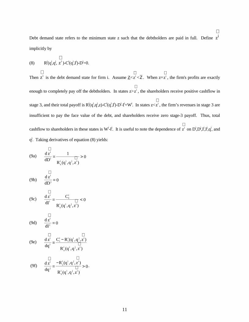
Debt demand state refers to the minimum state z such that the debtholders are paid in full. Define zi∧

implicitly by

(8) Ri(qi,qj, zi∧

)-Ci(qi,Ii)-Di=0.

Then zi∧

is the debt demand state for firm i. Assume Z<zi∧

<Ζ . When z=zi∧

, the firm's profits are exactly

enough to completely pay off the debtholders. In states z>zi∧

, the shareholders receive positive cashflow in

stage 3, and their total payoff is Ri(qi,qj,z)-Ci(qi,Ii)-Di-Ii+Wi. In states z<zi∧

, the firm’s revenues in stage 3 are

insufficient to pay the face value of the debt, and shareholders receive zero stage-3 payoff. Thus, total

cashflow to shareholders in these states is Wi-Ii. It is useful to note the dependence of zi∧

on Di,Dj,Ii,Ij,qi, and

qj. Taking derivatives of equation (8) yields:

(9a) d zdD

1

R (q ,q , z )0

i

i

zi i j i

∧

= ∧ >

(9b) d zdD

0i

j

∧

=

(9c) d zdI

C

R (q ,q , z )0

i

iIi

zi i j i

∧

= ∧ <

(9d) d zdI

0i

j

∧

=

(9e) d zdq

C R (q ,q , z )

R (q ,q , z )

i

iii

ii i j i

zi i j i

∧

=−

∧

∧

(9f) d zdq

R (q ,q , z )

R (q ,q , z )0

i

jji i j i

zi i j i

∧

=−

∧

∧ > .

12

The expression in (9a) is positive, so as firm i's debt level increases, its debt demand state increases. This is

not surprising given that revenue increases with the state variable z. Inequality (9c) is negative because

investment lowers the cost of producing any quantity, qi, while leaving the revenue function unchanged.

The expected value to the shareholders of firm i is

(10) V [R (q ,q , z) C (q ,I ) D ]f(z)dz I Wi i i j i i i iz

Z i ii= − − − +∧ .

The cashflow, Wi, has already been received by shareholders at the time of the quantity decision. Therefore,

the quantity choice at stage 3 will not affect this cashflow and, dWi/dqi=0. Assuming that each firm chooses

quantity to maximize the value of equity, each firm is maximizing equation (10). The first order condition

is: 16

(11) V [R (q ,q , z) c (q ,I )]f(z)dzii

ii i j i i i

z

Z

i= −∧ =0.

The first term of (11) is the expected marginal revenue received by firm i's shareholders when qi is

increased, and the second term is the expected marginal cost paid by firm i's shareholders when qi is

increased. The integral is over the states z in which there are residual claims for the shareholders. The

second order condition to guarantee a maximum is:

SOC: Viii<0.

Theorem 1a. An increase in debt, Di, by firm i causes an increase in their quantity, qi, and a decrease in the

competitor’s quantity, qj, i.e., dqdD

0i

i > and dqdD

0j

i < .

16The complete first order condition is:

Vii [Ri

i (qi , q j, z) ci (qi , Ii )]f(z)dzziZ [Ri (qi , q j , zi ) Ci (qi , Ii ) Di ]f(zi )

d zi

dqi 0= −∧ −∧

− −∧

∧

= ,

but the second half of the first order condition is zero by equation (8). Thus, equation (11) characterizes the quantity thatfirm i will choose.

13

Theorem 1b. If ViiI>0 then an increase in investment by firm i causes an increase in their quantity, qi, and a

decrease in the competitor’s quantity, qj. If ViiI<0 then an increase of investment by firm i has the opposite

effects, i.e., causes a decrease in their own quantity, qi, and an increase in the competitor’s quantity, qj.

Proof. See Appendix.

The first part of theorem 1 confirms that debt in this model has the same strategic effects that

Brander and Lewis discovered. The only one reason for a firm to have debt in this model is to commit to a

greater output. This strategic use of debt causes the competing firm to lower production in stage 3. When

firm i increases its debt, this increases the debt demand state, zi∧

, of firm i. Shareholders are only concerned

about states, z, where stage-3 profits are sufficient to repay the debtholders, i.e., z > zi∧

. Marginal revenue is

increasing in z, so when zi∧

increases, the marginal revenue relevant to shareholders also increases. With

higher marginal revenue, conditional on z>zi∧

, the firm will increase production. Firm i is committed to a

more aggressive product market position, and this causes the competitor to reduce output.

The second part of theorem 1 characterizes how investment affects the product market decision.

When a firm increases its investment, this has two effects on the product market decision. First, the firm

now has lower costs. With lower costs the firm has an incentive to increase production. This is the strategic

effect of investment analyzed by Brander and Spencer (1983). Second, due to lower costs of production the

firm is less likely to be bankrupt. When making the product market decision, the equity holders now care

about more states of demand, z, under which the firm has residual cash flow. Shareholders are now

optimizing over a larger set of possible states, and states where the marginal benefit of production is the

smallest are being added. This induces a desire for the firm to decrease the amount that it produces. The

sign of ViiI captures these two opposing effects and determines which one dominates.

14

IV Investment Choice Equilibrium

After the debt levels are determined and observed, the firms decide how much to invest in cost

reduction. Recall that investment lowers the marginal cost of production, which in turn can lower total

production costs. Investment is observed prior to the quantity choice of stage 3; thus, a firm can gain the

strategic advantage of having lower marginal cost through additional investment. When a firm is observed

to have a lower marginal cost, the rival will decrease their output, allowing the firm to increase both output

and expected profits.

The investment levels are chosen, taking the debt levels of each firm as given and correctly

anticipating the output market equilibrium that will occur in stage 3, which is the simultaneous solution of

each firm's first order condition in the quantity game, equation (11). The quantities both firms will choose

in stage 3 can be written as functions of the investment levels they chose in stage 2, i.e., qi=qi(Ii,Ij) and

qj=qj(Ii,Ij). Substituting these functions into the shareholder value equation yields expected profits to

shareholders as a function of investment. The firms choose investment levels to maximize the value of their

equity. The expected value to firm i shareholders when the firm invests Ii is

V [R (q (I ,I ),q (I ,I ), z) C (q (I ,I ), I ) D ]f(z)dz I Wi i i i j j i j i i i j i iz

Z i ii= − − − +∧ .

The term under the integral is the expected revenue firm i will earn net of debt payments. The minus Ii

reflects the fact that investment costs must be paid up front by the shareholders. The first order condition

for optimal investment is:17

(12) V [R (q ,q , z) C (q ,I )]f(z)dz 1 0Ii

Ii i j

Ii i i

z

Z

i= − − =∧

17For notational convenience the arguments to the quantity function are dropped. For the remainder of this

section qi=qi(Ii,Ij). Also note: RIi dRi

dqidqi

dIidRi

dq jdq j

dIi= + , and CIi dCi

dIidCi

dqidqi

dIi= + . There is an additional term in the

first order condition, −∧

− −

∧

[Ri (zi ) Ci Di ]d zi

dIi , which is zero by (4).

15

[R (q ,q , z) C (q ,I )]f(z)dz 1Ii i j

Ii i i

z

Z

i − =∧

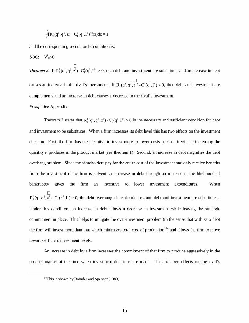
and the corresponding second order condition is:

SOC: ViII<0.

Theorem 2. If R (q ,q , z ) - C (q , I ) > 0Ii i j i

Ii i i

∧, then debt and investment are substitutes and an increase in debt

causes an increase in the rival’s investment. If R (q ,q , z ) - C (q , I ) < 0Ii i j i

Ii i i

∧, then debt and investment are

complements and an increase in debt causes a decrease in the rival’s investment.

Proof. See Appendix.

Theorem 2 states that R (q ,q , z ) - C (q , I ) > 0Ii i j i

Ii i i

∧ is the necessary and sufficient condition for debt

and investment to be substitutes. When a firm increases its debt level this has two effects on the investment

decision. First, the firm has the incentive to invest more to lower costs because it will be increasing the

quantity it produces in the product market (see theorem 1). Second, an increase in debt magnifies the debt

overhang problem. Since the shareholders pay for the entire cost of the investment and only receive benefits

from the investment if the firm is solvent, an increase in debt through an increase in the likelihood of

bankruptcy gives the firm an incentive to lower investment expenditures. When

R (q ,q , z ) - C (q , I ) > 0Ii i j i

Ii i i

∧, the debt overhang effect dominates, and debt and investment are substitutes.

Under this condition, an increase in debt allows a decrease in investment while leaving the strategic

commitment in place. This helps to mitigate the over-investment problem (in the sense that with zero debt

the firm will invest more than that which minimizes total cost of production18) and allows the firm to move

towards efficient investment levels.

An increase in debt by a firm increases the commitment of that firm to produce aggressively in the

product market at the time when investment decisions are made. This has two effects on the rival’s

18This is shown by Brander and Spencer (1983).

16

investment decision. The competing firm knows it will face more aggressive competition in the product

market, which results in lower revenues in all states of the world; this causes the rival to reduce investment.

The competing firm also knows that it will be facing a firm which invests less, which causes the competitor

to increase investment. The latter effect dominates when R (q ,q , z ) - C (q , I ) > 0Ii i j i

Ii i i

∧. If

R (q ,q , z ) - C (q , I ) < 0Ii i j i

Ii i i

∧, then the former effect dominates and debt and investment are complements.

In this case, an increase in the debt of firm i causes an increase in investment for firm i, and a decrease in

investment for firm j.

Theorem 3. If marginal revenue is positive then debt and investment are substitutes.19

Proof. See Appendix.

Theorem 3 states that a sufficient, but not necessary, condition for debt and investment to be substitutes

is that marginal revenue is positive. Although we do not expect this condition to always hold, there are

situations when we expect Rii>0, and the condition, R (q ,q , z ) - C (q , I ) > 0I

i i j iIi i i

∧, may still hold when

marginal revenue is not positive.

V Debt Choice Equilibrium

In stage 1 the firms choose debt levels simultaneously. These debt levels are chosen with the

knowledge of how they will affect both the quantity equilibrium and the investment equilibrium, which are

the simultaneous solutions to each firm's first order conditions, equations (11) and (12) respectively. The

buyers of debt have perfect information, and there is a competitive market for the sale of debt. Wi is the fair

19Moreover, if marginal revenue is positive at the relevant debt demand state then debt and investment are

substitutes (see proof).

17

market value of the debt issued. Wi will be the expected payoff to debt holders given the face value of each

firm’s debt, Di and Dj, and how those debt levels will affect the investment and quantity choice of each firm.

Let D = (Di,Dj). Then each firm’s investment level can be written as a function of D, i.e., Ii(D). Let I =

(Ii(D),Ij(D)). Then each firm’s quantity choice can be written as a function of D. Substituting these

relations into equation (10), yields the expected value to shareholders expressed as a function of debt levels:

V [R (q (D),q (D), z) C (q (D),I (D)) D ]f(z)dz I (D) Wi i i j i i i iz

Z i ii= − − − +∧ .

Similarly, Wi can be expressed as a function of debt levels as follows:

W [R (q (D),q (D), z) C (q (D),I (D))]f(z)dz D (1 F(z ))i i i j i i iZ

z i ii

= − + −∧∧

The term under the integral of Wi is the profits of firm i. This is integrated over the states of nature when

the firm is bankrupt. In these states the debtholders receive all of the firm's profits. The second term is the

cashflow received by debtholders when the firm can completely pay its debt obligations (the face value of

the debt) multiplied by the probability that the firm will be solvent. Note that [D ]f(z)dz D (1 F(z ))iz

Z i ii

∧ = −∧

,

which implies that

V [R (q (D),q (D), z) C (q (D),I (D))]f(z)dz I (D) [R (q (D),q (D), z) C (q (D),I (D))]f(z)dzi i i j i i iz

Z i i i j i i iZ

z

i

i

= − − + −∧

∧

.

Firm i maximizes Vi with respect to the choice of debt level. The first order condition is20

(13) FOC: dVdD

i

i

(13.1) = −∧[ [R (q ,q , z) c (q ,I )]f(z)dz]dqdDi

i i j i i iz

Zi

ii

(13.2) + −∧

[ [R (q ,q , z) c (q ,I )]f(z)dz]dqdDi

i i j i i iZ

zi

i

i

20Note that I can be written as a function of D, and q can be written as a function of D and I, which can

further be represented as just a function of D. Once q is expressed solely as a function of D (incorporating theimplicit change in I) the following first order condition is correct.

18

(13.3) + +∧

∧

[ R (q ,q , z)f(z)dz R (q ,q , z)f(z)dz]dqdDj

i i jz

Z

ji i j

Z

zj

ii

i

(13.4) + − −∧[ [R (q ,q , z) C (q ,I )]f(z)dz 1]dIdDI

i i jIi i i

z

Zi

ii

(13.5) + −∧

[ [R (q ,q , z) C (q ,I )]f(z)dz]dIdDI

i i jIi i i

Z

zi

i

i

(13.6) + +∧

∧

[ R (q ,q , z)f(z)dz R (q ,q , z)f(z)dz]dIdDJ

i i jz

Z

Ji i j

Z

zj

ii

i

= 0.

The first and fourth terms of (13) are zero by equations (11) and (12) respectively. The second term,

(14) [ [R (q ,q , z) c (q ,I )]f(z)dz]dqdDi

i i j i i iZ

zi

i

i

−∧

,

is the change in the value of the debt caused by the induced change in qi. This is the additional agency cost

of adding debt due to the change in quantity that firm i chooses. Rii(.)-ci(.) is the change in profits caused by

a change in qi. This is integrated over the states, z, in which the firm is in default to determine the expected

change in debt value when qi changes. In the demand states in which the firm is bankrupt the change in the

value of the debt is the change in profits (revenue - costs) since here the debtholders receive all of the firm’s

profits.21 This is multiplied by the change in qi caused by a change in Di, dqdD

i

i . This term is less than zero

by theorem 1 and equation (11), along with the assumption that Riiz>0. Theorem 1 states that dqi/dDi > 0.

Equation (11), along with the assumption that Riiz>0, implies that

Rii(qi,qj, zi

∧ ) - ci(qi,Ii) < 0.

Equation (11) states that the integral from zi∧

to Z of Rii(.) - ci(.) is equal to zero. Since marginal revenue

is increasing in z and marginal cost is constant in z, it must be the case that Rii(.) - ci(.)<0 at zi

∧. As z

21In states where the firm is not bankrupt a change in the firm’s quantity does not affect the payoff to

debtholders since they receive the same payoff, the face value of debt, regardless of the profits of the firm.

19

decreases below zi∧

, the value of the above equation decreases further; therefore, Rii(.) - ci(.)<0 for all z ≤

zi∧

. This confirms that equation (14) is less then zero, which means that an increase in debt magnifies the

conflict between debtholders and equityholders with respect to desired quantity choice. When a firm

increases its debt this induces an increase in the quantity produced. The firm chooses quantity to maximize

equity value, and thus this is the quantity that is best for the shareholders. As shown above this increase in

quantity decreases the debt value of the firm. The difference between the quantity that would maximize the

debt value and the quantity that would maximize the equity value is increasing as the debt level increases.

The third term is the change in value to equityholders and debtholders caused by the induced

change in qj. This is the strategic value of additional debt on the quantity game. The first integral is the

change in the equity value of the firm and the second integral is the change in the debt value of the firm.

(15) R (q ,q , z)f(z)dzdqdD

R (q ,q , z)f(z)dzdqdDj

i i jz

Zj

i ji i j

Z

zj

ii

i

∧

∧

+

= [ R (q ,q , z)f(z)dz]dqdDj

i i jZ

Zj

i .

Equation (15) is the strategic effect of debt on the quantity game. Since an increase in debt by firm i causes

qj to decrease (from theorem 1), and Rij<0 by assumption (1a) both terms of equation (15) are greater than

zero. The strategic effect of debt causes the rival firm to decrease their output which increases both the debt

value and the equity value of the firm.

The fifth term is

(16) [R (q ,q , z) C (q ,I )]f(z)dzdIdDI

i i jIi i i

Z

zi

i

i

−∧

,

which is the change in agency costs of debt on the investment game. This term can be positive or negative

since the induced change in investment can make the debtholders either better or worse off. Thus,

increasing debt can either increase of decrease the conflict between debt and equity over the desired choice

20

of investment. RiI - Ci

I is the change in profits caused by a change in investment. This is integrated over the

states where the firm is bankrupt to get the expected change in profits, from a change of investment, in the

states where the debt holders receive all the profits. This is multiplied by the change in investment induced

by a change in debt. This yields the change in the debt value of the firm from the induced change in Ii. If

marginal revenue in stage 3 is positive then (16) is negative, and under this condition an increase in debt

also exacerbates the conflict between shareholders and debtholders with respect to the optimal investment

choice. If equation (16) is positive then an increase in debt reduces the agency costs from the conflict

between debt and equity over the choice of investment level and this reduction in agency costs increases

firm value.

The last term is

(17) R (q ,q , z)f(z)dzdIdD

R (q ,q , z)f(z)dzdIdDJ

i i jz

Zj

i Ji i j

Z

zj

ii

i

∧

∧

+

= R (q ,q , z)f(z)dzdIdDJ

i i jZ

Zj

i ,

which is the strategic value of additional debt on the investment game. RiJ is the change in revenues to firm

i from a change in the investment of the rival. The first term of (17) is the change in revenues when the firm

is solvent, and the second term is the change in revenues when the firm is bankrupt. This is the effect of the

induced change in Ij on the equity and debt value of firm i respectively. If marginal revenue is positive then

an increase in debt by firm i causes firm j to increases investment which decreases the equity value and the

debt value of firm i. This can been seen by observing that the final term of equation (13) is negative when

Rii>0.22

22 RJ

i Rii dqi

dI j R ji dq j

dI j Rzi dz

dI j 0= + + < when Rii>0, because Ri

j<0 by (1a), and dz

dI j 0= (see footnote 12). The

result follows from theorem 1. The sign of equation (17) follows from theorem 2.

21

When marginal revenue is positive then increasing the face value of debt has four effects on the

value of the firm, three which lower the value of the firm and one which raises the value of the firm. More

debt lowers the value of the firm by increasing the conflict between debt and equityholders with regard to

the desired choice of investment and quantity. Debt also lowers the value of the firm through the effect on

the competition’s choice of investment. When the firm increases its debt level the rival increases its

investment which lowers the value of the firm. An increase in debt raises the value of the firm through the

effects on the competition’s choice of quantity. In particular, an increase in debt causes the competition to

decrease quantity. When the firm's debt level is small, the conflict between debtholders and equityholders is

insignificant, and the negative effect of an increase in debt due to these conflicts is negligible. Specifically,

when D=0 there are no debtholders, and therefore no conflict between the claimants. This becomes evident

from examining equations (14) and (16) and noting that D=0 implies that zi∧

=Z; therefore, equations (14)

and (16) are both equal to zero. Increasing debt from zero has two effects on firm value. Firm value is

increased due to the decrease in rival output. Firm value is decreased due to the increase in rival

investment.23

VI Increasing Demand

This section examines how an arbitrary shift in the distribution of demand changes each of the

individual effects characterized in section V. The effects are examined by holding all other variables

constant and determining how each term changes as the underlying distribution of demand is increased.

Let g(.) be the probability density function of a random variable distributed continuously on [Z’,

Z’]. Assume that the distribution g(.) dominates f(.) in the sense of First Degree Stochastic Dominance.

23Recall that in this case it is assumed that marginal cost is positive, thus debt and investment are

substitutes.

22

This means for any z, G(z) ≤ F(z), which implies that Z’≥ Z and Z’≥ Z . First consider the agency costs of

debt on the quantity game, which is equation (14)

(14) [ [R (q ,q , z) c (q ,I )]f(z)dz]dqdDi

i i j i i iZ

zi

i

i

−∧

.

For each state z < zi∧

the term under the integral in equation (14) is negative and increasing in z. If the

distribution of demand is shifted to g(.) then equation (14) becomes

(14’) [ [R (q ,q , z) c (q ,I )]g(z)dz]dqdDi

i i j i i iZ'

zi

i

i

−∧

.

Equation (14’) is larger than equation (14) because the term under the integral is negative, increasing in z,

and g(.) dominates f(.). This means that if the support of demand increases ex ante the agency cost of debt

on the quantity decision is reduced. Note that in the extreme case as demand increase to the point of the

debt becoming riskless the agency cost of debt goes to zero, as expected.

Second examine the strategic value of debt on the quantity game, equation (15),

(15) = [ R (q ,q , z)f(z)dz]dqdDj

i i jZ

Zj

i .

When the distribution of z is shifted to g(.), then equation (15) becomes

(15’) = [ R (q ,q , z)g(z)dz]dqdDj

i i jZ'

Z'j

i .

Whether equation (15’) is larger or smaller than (15) depends on the sign of Rijz, i.e., whether the integrand

is increasing or decreasing in z. Recall that Rij is negative, that is, as firm j increase its output the revenue to

firm i falls. The sign of Rijz tells us whether the revenue of firm i falls more or less in reaction to an increase

of rival output when demand is higher. If Rijz > 0, which means that when demand is higher an increase in

rival output decrease own firm revenue by less than when demand is lower, then the strategic value of debt

is smaller when demand increases. The strategic value of debt is the effect of committing to a large output

and therefore inducing the rival firm to decrease its output. If a reduction in rival output increase own firm

23

revenue by less (which it does when demand is higher and Rijz > 0) then the strategic value of debt

decreases. If, on the other hand, Rijz < 0 then the strategic value of debt is larger when demand is higher.

Higher demand may increase or decrease the agency costs associated with the investment choice,

equation (16), and the result depends on several parameters. For instance if ViI > 0 and RiI>0 then it must be

the case that RiI(.)-Ci

I>0 at zi∧

(since RiI(.)-Ci

I>0 when RiI>0 and Ci

I<0 (from 2a)). From theorem 2 RiI(.)-

CiI>0 implies that dIi/dDi<0. In this situation equation (16) is negative so an increase in debt magnifies the

conflict between debt and equity holders over the optimal investment choice. Under these conditions the

agency costs of debt associated with the investment choice decreases when demand is higher. Under

different initial conditions, however, it is possible that these agency costs increase when demand is higher.

The change in the strategic value of debt on the investment game, equation (17), depends on the

sign of RiJz, and dIj/dDi. If Ri

Jz<0 (RiJz>0), which means that as the realization of demand, z, increases the

revenue received by firm i decreases (increases) as the competitor increases their investment spending, and

dIj/dDi<0 (dIj/dDi>0), which means that as firm i increases its debt level this induces the competitor to

decreases (increases) their investment, then as demand increases the strategic value of debt on the

investment decision increases (decreases).

VII Numerical Examples

To better understand how the choice variables change in equilibrium with variation in the

distribution of z, I have computed equilibria in numerical examples with discrete random demand. I assume

that the firms produce identical goods, and that the inverse demand function is

P = A[z] - q1 - q2.

There are seven equally likely states of demand, z = 1, 2, ..., 7, with A[z] increasing with z. The cost of

production for firm i is Ci(qi,Ii) = (40− Ii )qi.

24

First I examine how equilibrium decisions change as demand increases. These examples show that

as demand increases the equilibrium investment and quantities increase. The equilibrium debt level,

however, does not move monotonically as demand increases. Second I examine how the equilibrium

decisions change as the variance of demand states increases. It is assumed that the variance increases

through a mean preserving spread. When the variance of demand increases the equilibrium quantities

increase. This is the only variable that changes monotonically when the uncertainty about demand

increases.

Increasing Demand

I first examine the case of increasing demand. These results are reported in table I. In case 1, the

seven possible states of demand are 90, 95, 100, 105, 110, 115, and 120. Case 1 has a unique symmetric

sequential Nash equilibrium in debt demand state, investment, and quantity. Demand is discrete, and

consequently there is a range of possible debt levels that will support each debt demand state. In

equilibrium, firms issue debt such that the debt demand state is demand state z=3 or A(z)=100. For this to

occur, D must belong to the interval [430.25, 491.83]. The equilibrium investment level is I=174.44, and

the equilibrium quantity is q=27.74. Given these choices, the expected price is 49.53, and each firm's

expected profit is $456.16.

In case 2, demand increases by one over the case 1 values in each state. Case 2 demands are 91, 96,

101, 106, 111, 116, and 121. As demand increases from case 1 to case 2, the equilibrium debt demand state

remains constant. The expected demand relevant to shareholders (E[ A(z) | z ≥ 3 ]) increases from 110 to

111. This generates an increase in investment to 179.46 and quantity to 28.13. The debt levels that support

this equilibrium increase to the interval [450.07, 510.28]. Expected price and expected profits are also up to

49.74 and $471.29 respectively. In this example an increase in demand increases all endogenous choice

variables, expected price, and expected profits.

25

Case 3 has demand again increasing by one in each state. Case 3 demands are 92, 97, 102, 107,

112, 117, and 122. Due to this increase in demand, the debt demand state decreases from 3 to 2. Any debt

levels within the interval [405, 461.07] support the equilibrium. This interval is below the case 2

equilibrium, which shows that the minimum and maximum debt levels that support the equilibrium are not

monotonic in level of demand. Investment and quantities are up to 267.42 and 28.62 respectively. The

large jump in investment spending is due to the fact that debt and investment are substitutes for

commitment. By lowering the commitment of debt in stage 1 the firms now try to commit more with

investment in stage 2. The fact that most of the additional investment spending is for commitment can be

seen by examining the optimal investment levels in case 2 and case 3. In case 2, actual investment is just

below optimal investment, while in case 3, actual investment in significantly above optimal investment.

The only explanation for investing higher than optimal levels is to commit to an aggressive product market

position in stage 3. Expected price is up slightly to 49.76 and expected profits are up to $480.

In Case 4, the demand states are 91.5, 96.5, 101.5, 106.5, 111.5, 116.5, and 121.5. These demand

levels are between case 2 and case 3 demand levels. This case has two symmetric sequential Nash

equilibria, which allows us to examine how the endogenous variables react when only the debt demand state

changes. Obviously, the support of equilibrium debt levels decreases when the debt demand state falls. The

firm now uses debt to eliminate a lower number of demand states, and, therefore, less debt is needed. The

firm increases investment in an attempt to make up for the commitment lost by the lower debt. Firms over-

invest in the second equilibrium. Although shareholders are now concerned about a lower demand state,

quantity increases. This is due to the large increase in investment, which simultaneously lowers marginal

cost and increases commitment. Both of these effects induce larger outputs by the firm.

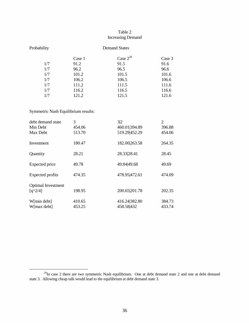
Table 2 shows cases of increasing demand around the case with two equilibria. Moving from case

1 to case 3 yields the unexpected result that an increase in demand can create a decrease in both price and

expected profits. This is caused by the firms' increase in investment spending. In case 3 the firms’ debt

26

demand state drops to z=2 from z=3 in case 1. To compensate for the loss of commitment from stage 1, the

firms now use investment strategically. Investment increases from 180.47 to 264.35, which is a move from

under-investment to over-investment. This over-investment eliminates any gains in profits that would

otherwise have been realized from an increase in demand.

These examples show that an increase in demand has monotonic effects on both investment and

quantity choices. The interval of debt levels that support the equilibria, however, does not move

monotonically as demand increases. The investment result will generalize due to the fact that all the effects

on investment as demand increases are positive. The quantity result may not be robust. As demand

increases, the debt demand state decreases. This implies that the shareholders must now consider lower

states of demand when choosing quantity. This has the direct consequence of lowering the desired quantity.

The increase in investment has two indirect effects,24 both of which increase the desired quantity. There is

no reason to believe that the direct effect cannot dominate for some parameter values.

For comparison Table 5 examines the case of no investment. This is the Brander and Lewis model.

The equilibrium debt demand state is state 6. As demand increases, the maximum and minimum elements

of the support of equilibrium debt levels increase. Quantity also increases with demand. Expected price

and expected profits also rise. Table 6 considers the case with no debt. This is the Brander and Spencer

model. Here the debt demand state is 1 (since there is no debt). As demand increases, investment and

quantity increase. Expected price and expected profits also increase.

Changes in Demand Variance

Table 3 illustrates how the decision variables change as the variance of demand increases. The

variance is increased through a mean preserving spread. The average demand in each case is 100. The

24 Investment lowers the marginal cost of production, which causes an increase in quantity. Investment also

causes the competing firm to lower its production, which also causes an increase in own quantity.

27

probabilities of each state remain the same, while the support of possible demand states increases. As the

variance of the demand states increases, the value of committing with debt increases. When the variance is

high then the expected demand realization conditional upon z > zi∧

is larger than when the variance is small.

The firm chooses investment and quantity based on expected demand conditional on the firm having

enough profits to pay back the debt. Thus, when the variance of demand is high the same level of debt

commits the firm to more aggressive output market decisions than when demand variance is low. This

increases the relative propensity of firms to use debt instead of investment as a commitment device. This is

why as the variance of demand increases we see the debt demand state increasing and investment

decreasing.

In this example as variance increases, investment, expected price, and expected profits decrease,

while quantity increases. Debt levels are not monotonic in the variance of demand. As the variance

increases, the equilibrium debt demand state rises. This precipitates a lower investment level due to the fact

that debt and investment are substitutes for strategic commitment. The quantity produced increases due to

the increase in expected demand relevant to shareholders. This has a direct positive effect on investment

levels, as an increase in quantity makes more investment favorable. In these cases, the commitment effect

dominates.

These examples, however, all have sufficiently large increases in the variance to produce an

increase in the equilibrium debt demand state. Table 4 examines increases in the variance where the debt

demand state remains constant. Here we see that the monotonicity of quantity, expected price, and expected

profit remain intact; however, investment is increasing rather than decreasing over these cases. This

increase in investment is due to the fact that quantity increases, but the debt demand state remains the same,

so there is no negative effect on investment.

From these limited examples, quantity is the only decision variable that is monotonically increasing

in variance. These examples allow the support of the demand distribution to move. If the variance of

28

demand increases with the support remaining constant, we may see more decision variables changing

monotonically.

VIII Extensions

There are two natural modifications of this model which are worthwhile to investigate. First, it is

interesting to examine how debt and investment interact when the order of the decision variables are

changed. For instance, a similar model where the firms first choose investment levels and then choose

capital structure can be investigated. Second, it is natural to be curious about whether the results of this

model are robust to different types of product market competition.

Consider a model where first, firms choose investment levels; second, firms choose capital

structure; and finally, firms compete under Cournot competition in the product market. First note that from

the point in the game where firms choose capital structure to the end game, the game is exactly the same as

that developed by Brander and Lewis.25 The firms will always choose positive debt levels due to the

strategic effect of debt on the product market.

Investment affects both the product market decision and the capital structure decision. Investment

has a strategic effect on the product market decision. Brander and Spencer demonstrated that by lowering

the cost of production, the firm will be committed to producing more in the product market. Investment has

two effects on the capital structure stage (both of these effects have consequences on the product market

stage indirectly). First, investment lowers the cost of production. This decreases the agency costs of debt in

two ways. With lower costs of production there is an increase in stage-3 cashflow available to distribute to

claimants, regardless of the state of demand; thus, ceteris paribus the value of the debt increases.26 With

25 At the stage when the firms are making their capital structure decision, investment is fixed and thus this

subgame reduces to the game developed by Brander and Lewis.

26 Recall that investment is paid for up front and excess cash is distributed to shareholders, thus an increasein investment only increases cash flow in the final stage through lower costs of production.

29

lower agency costs, the firm would want to increase the amount of debt issued (as long as the benefits of the

debt are not changed). Second, investment can change the strategic commitment value of debt. Whether

investment increases or decreases the commitment value of debt depends on second derivatives. If the

strategic value of debt is increased through lower costs, then debt and investment will always be

compliments. If lower costs decrease the strategic value of debt, then debt and investment can be

substitutes.

The second interesting extension is to investigate the model with Bertrand competition in the

product market. It is well known that many results of theoretical models change when the type of product

market competition is changed from Cournot to Bertrand. This is due to the fact that in Cournot

competition the firms choices are substitutes, where in Bertrand competition the firms choice variables are

complements.

How would the interaction of debt and investment behave if the original model were changed so the

firms first choose capital structure, second choose investment, and third compete with prices in the product

market? Debt has only a strategic effect on the product market in this model. Showalter (1995) shows that

if the Brander and Lewis model is changed to Bertrand competition in the product market, then an increase

in debt causes both firms to increase price (and thus decrease quantity produced). Debt is still used

strategically, but instead of committing the firms to aggressive output market positions, debt allows the

firms to coordinate on high prices. This is the opposite of the result with Cournot competition.

Debt has two effects on the investment choice. An increase in debt leads to lower production which

makes the firm want to invest less. More debt also magnifies the debt overhang problem which also leads

the firm to decrease its investment. Hence, with Bertrand competition, debt and investment are substitutes.

This result may also be obtained from the original model; thus, changing from Cournot to Bertrand

competition may not affect the interaction between the capital structure and the investment choice.

30

IX Conclusion

This paper illustrates how capital structure, investment, and product market decisions are

interrelated. The results obtained when modeling the interaction of only two of these choices may be

reversed when the third choice variable is introduced. These decisions are analyzed under a specific

structure where the decisions are assumed to occur sequentially. First, financial structure is chosen, second,

investment is chosen, and finally, firms choose quantities to be distributed to the product market. Under this

configuration, the financial structure decision has an effect on both the investment and the product market

stages of the game. These effects are due to the limited liability of equity. In the product market, debt

commits the firm to an aggressive output decision, causing an increase in own output and a decrease in

rival’s output. Debt has two effects on the investment decision. First, the firm increases output, which

raises the marginal benefit of lower marginal cost, and thus the firm wants to increase investment. Second,

investment is used strategically as a commitment to high outputs in the product market. The complete effect

of debt on investment depends on whether investment and debt are substitutes or compliments for

commitment in the product market.

This paper provides necessary and sufficient conditions for debt and investment to be substitutes.

For example, when investment is paid for by shareholders, debt and investment are substitutes if marginal

revenue is positive. This mitigates the over-investment result obtained by Brander and Spencer (1983).

In addition, this paper demonstrates how recent empirical evidence on the relation between debt,

investment, and product market behavior can be consistent with a model emphasizing the limited liability of

equity. This framework is perhaps more palatable than the predatory theories because firms rationally take

on debt. Whereas in the predatory models the optimal debt level is zero. Further research is necessary to

distinguish between these two theories.

31

APPENDIX

Proof of theorem 1.Totally differentiate equation (11) and the corresponding first order condition for firm j with respect

to qi, qj, and Di. This gives the following equations:Vi

iidqi+Viijdqj+Vi

iDdDi=0Vj

jidqi+Vjjjdqj+Vj

jDdDi=0.

Note: VjjD = -[Rj

j(qi,qj, z∧

i)-Cjj(qj,Ij)]d z

∧j/dDi = 0, because d z

∧j/dDi = 0 (see equation (9b)). Thus, the

equations simplify toVi

iidqi+Viijdqj=-Vi

iDdDi

Vjjidqi+Vj

jjdqj=0.Solving these equations simultaneously gives:(A1) dqi/dDi = -Vj

jjViiD/A where A=Vi

iiVjjj-Vi

ijVjji

(A2) dqj/dDi = VjjiVi

iD/AA>0 by assumption, Vj

jj<0 by SOC, Vjji<0 by (4), so the signs of the above equations are determined by the

sign of ViiD.

ViiD = -[Ri

i(qi,qj, z∧

i)-ci(qi,Ii)]f( z∧

i)d z∧

i/dDi

Equation (9a) shows that d z∧

i/dDi > 0. Riiz>0 by assumption, this means that as z increases marginal revenue

increase. This along with the fact that the first order condition (equation (11)) is satisfied guarantees that

[Rii(qi,qj, z

∧ i)-ci(qi,Ii)] < 0 (i.e., at z

∧i marginal revenue is less than marginal cost). This means that Vi

iD > 0,which implies that equation (A1) > 0 and (A2) < 0.

To derive dqi/dIi and dqj/dIi totally differentiate (11) with respect to qi, qj, and Ii. Also totallydifferentiate the corresponding FOC for firm j with respect to the same variables (i.e., qi, qj, and Ii). Thisyields the following equations:

Viiidqi+Vi

ijdqj+ViiIdI=0

Vjjidqi+Vj

jjdqj+VjjIdI=0

Note using Leibnitz's rule: VjjI =

z

Z

j∧

[RjjI(q1,q2,z)-cj

I(qi,Ii)]f(zj)dz - [Rii(q1,q2,z)-ci(qi,Ii)]f( z

∧j)d z

∧j/dI = 0 because

firm j's revenue and cost function are not effected by firm i's investment (so RjjI = 0 and Cj

jI = 0) and d z∧

j/dI

= 0 by (9d). ViiI =

z

Z

i∧

[RiiI(q1,q2,z)-ci

I(qi,Ii)]f(z)dz - [Rii(q1,q2,z)-ci(qi,Ii)]f( z

∧i)d z

∧i/dI. Firm i's revenue does not

depend on its investment (i.e., RiiI = 0) and firm i's cost are not dependent on the state of the world (ci

I

constant across states z), thus ViiI = -(f(Ζ )-f( z

∧i))ci

I(qi,Ii) - [Rii(q1,q2,z)-ci(qi,Ii)]f( z

∧i)Ci

I/Riz(q1,qj, z

∧i). This

leaves the following equations:

Viiidqi+Vi

ijdqj=[(f(Ζ )-f( z∧

i))ciI + [Ri

i(q1,q2,z)-ci(qi,Ii)]f( z∧

i)CiI/Ri

z(q1,qj, z∧

i)]dIi

Vjjidqi+Vj

jjdqj=0Solving these equations simultaneously yields

(18) dqi/dIi=Vjjj[(f(Ζ )-f( z

∧i))ci

I+[Rii-ci]f( z

∧i)Ci

I/Riz( z

∧i)]dIi/A where A=Vi

iiVjjj-Vi

ijVjji

(19) dqj/dIi=-Vjji[(f(Ζ )-f( z

∧i))ci

I+[Rii-ci]f( z

∧i)Ci

I/Riz( z

∧i)]dIi/A

Equation (18) is greater than zero if ViiI>0 (or equivalently if - (Ζ - z

∧i)ci

I > [Rii-ci]f( z

∧i)Ci

I/Riz]) because A>0

by assumption, Ζ> z∧

i, ciI<0 by (2d), and Vj

jj<0 by SOC.

32

Equation (19) is the opposite sign of equation (18) because Vjji<0 see equation(4). QED

Proof of theorem 2.To solve for dI/dDi and dJ/dDi first totally differentiate (12) with respect to Ii, Ij, Di. We also totally

differentiate the corresponding FOC VjJ with respect to the same variables. This yields the following

equations:Vi

IIdI+ViIJdJ+Vi

IDdDi=0Vj

JIdI+VjJJdJ+Vj

JDdDi=0.V R (q ,q , z) - C (q , I )]f(z)dzJ

jJj i j

Jj j j

z

Z

j= ∧ [

dVjJ/dDi=-[Rj

J(qi,qj, z∧

i)-CjJ(qj,IJ)]d z

∧j/dDi=0 because d z

∧j/dDi=0.

Thus the resulting equations areVi

IIdI+ViIJdJ=-Vi

IDdDi

VjJIdI+Vj

JJdJ=0Solving these equations using simultaneously yields(20) dI/dDi=-Vi

IDVjJJ/B where B=Vi

IIVjJJ-Vi

IJVjJI

(21) dJ/dDi=ViIDVj

JI/B.We know Vj

JJ<0 by (SOC) and B>0 by (7), so the sign of dIi/dDi is the same as the sign of ViID. Solving for

ViID gives

ViID=-[Ri

I(qi,qj, z∧

i)-CiI(qi,Ii)]f( z

∧i)d z

∧i/dDi.

d z∧

i/dDi>0 from (9a). Whenever [R (q ,q , z ) - C (q ,I )Ii i j i

Ii i i

∧] > 0 then Vi

ID<0 and dIi/dD<0, alternatively

whenever [R (q ,q , z ) - C (q ,I )Ii i j i

Ii i i

∧] < 0 then Vi

ID>0 and dI/dD>0. From (5) VjJI<0 thus dIj/dD is the

opposite sign of dI/dD from (20) and (21).

Notice that if [R (q ,q , z ) - C (q ,I )Ii i j i

Ii i i

∧] = 0 Vi

ID = 0 and thus (20) and (21) are both equal to zero. Whichmeans that a change in debt of firm i has no effect on the investment of either firm.

Proof of theorem 3.

Note CiI<0 by (2a), thus [R (q ,q , z ) - C (q ,I )I

i i j iIi i i

∧] > 0 whenever Ri

I(qi,qj, z∧

i)>0. RiI(qi,qj, z

∧ i ) is the change

in revenue in the worst state of the world that is relevant to shareholders when investment increases.

RiI(qi,qj, z

∧ i)=Ri

i(qi,qj, z∧

i)dqi/dIi+Rij(qi,qj, z

∧i)dqj/dIi

Observe that dqi/dIi>0 dqj/dIi<0 by equation(18) and equation(19) respectively and ViiI>0 by assumption.

Thus whenever Rii>0 this implies that [R (q ,q , z ) - C (q ,I )I

i i j iIi i i

∧] > 0. In fact even if

Rii<0, if Ri

i(qi,qj, z∧

i)dqi/dIi ≥ - Rij(qi,qj, z

∧i)dqj/dIi then [R (q ,q , z ) - C (q ,I )I

i i j iIi i i

∧] > 0 still holds. Actually

even if Rii(qi,qj, z

∧i)dqi/dIi < - Ri

j(qi,qj, z∧

i)dqj/dIi, if RiI(qi,qj, z

∧ i)> Ci

I(.) then [R (q ,q , z ) - C (q ,I )Ii i j i

Ii i i

∧] > 0

still holds. Although we don’t expect this condition to always hold there are many situations when weexpect Ri

i>0 and the condition still holds in many circumstances when marginal revenue is not positive, thuswe do expect this condition to be satisfied in many instances.

33

References

Bolton, P. and D. Scharfstein, 1990, ‘‘A Theory of Predation Based on Agency Problems in FinancialContraction,’’ American Economic Review 80: 93-106.

Brander, J., and T. Lewis, 1986, ‘‘Oligopoly and Financial Structure: The Limited Liability Effect,’’American Economic Review 76: 956-970.

Brander, J., and B. Spencer, 1983, ‘‘Strategic commitment with R&D: the symmetric case,’’ Bell Journal ofEconomics 14: 225-235.

Chevalier, J., 1995, ‘‘Capital Structure and Product-Market Competition: Empirical Evidence from theSupermarket Industry,’’ American Economic Review 85: 415-435.

Fershtman, C., and K. Judd, 1987, ‘‘Equilibrium Incentives in Oligopoly,’’ American Economic Review 77:927-940.

Fulghieri, P., and S. Nagarajan, 1991, ‘‘Financial Contracts as Lasting Commitments: The Case of aLeveraged Oligopoly,’’ Journal of Financial Intermediation 2: 2-32.

Hart, O., and J. Tirole, 1988, ‘‘Contract Renegotiation and Coasian Dynamics,’’ Review of EconomicStudies 55: 509-540.

Holmstrom, B., and R. Myerson, 1983, ‘‘Efficient and Durable Decision Rules with IncompleteInformation,’’ Econometrica 51: 1799-1819.

Jensen, M., and H. Meckling, 1976, ‘‘Theory of the Firm: Managerial Behavior, Agency Costs andOwnership Structure,’’ Journal of Financial Economics 3: 305-360.

Kaplan, S., 1989, ‘‘The effects of management buyouts on operating performance and value,’’ Journal ofFinancial Economics 24: 217-254.

Kovenock, D., and G. Phillips, 1994, ‘‘Capital Structure and Product Market Behavior: An Examination ofPlant Exit and Investment Decisions,’’ mimeo, Purdue University.

Kovenock, D., and G. Phillips, 1995, ‘‘Capital Structure and Product Market Rivalry: How Do WeReconcile Theory and Evidence?,’’ American Economic Review

Kreps, D., and R. Wilson, 1982, ‘‘Sequential Equilibrium,’’ Econometrica 50: 863-894.

Maksimovic, V., 1988, ‘‘Capital Structure in Repeated Oligopolies,’’ Rand Journal of Economics 19: 389-407.

Myers, S., 1977, ‘‘Determinants of Corporate Borrowing,’’ Journal of Financial Economics 5: 147-175.

Modigliani, F., and M. Miller, 1958, ‘‘The Cost of Capital, Corporation Finance, and the Theory ofInvestment,’’ American Economic Review 48: 261-297.

34

Phillips, G., 1995, ‘‘Increased debt and industry product markets An empirical analysis,’’ Journal ofFinancial Economics 37: 189-238.

Poitevin, M., 1989, ‘‘Financial signaling and the “deep-pocket” argument,’’ Rand Journal of Economics 20:26-40.

Rotemberg, J., and D. Scharfstein, 1990, ‘‘Shareholder-Value Maximization and Product MarketCompetition,’’ Review of Financial Studies 3: 367-391.

Selten, R., 1965, ‘‘Spieltheoretische Behandlung eines Oligopolmodells mit Nachfragetragheit,’’ Zeitschriftfur die gesamte Staatswissenschaft 121: 301-324.

________, 1975, ‘‘Re-examination of the Perfectness Concept for Equilibrium Points in Extensive Games,’’International Journal of Game Theory 4: 25-55.

Showalter, D., 1995, ‘‘Oligopoly and Financial Structure: Comment,’’ American Economic Review 85:647-653.

Sklivas, S., 1987, ‘‘The Strategic Choice of Managerial Incentives,’’ Rand Journal of Economics 18: 452-458.

35

Table 1Increasing Demand

Probability Demand States

Case 1 Case 2 Case 427 Case 31/7 90 91 91.5 921/7 95 96 96.5 971/7 100 101 101.5 1021/7 105 106 106.5 1071/7 110 111 111.5 1121/7 115 116 116.5 1171/7 120 121 121.5 122

Symmetric Nash Equilibrium results:

debt demand state 3 3 3|2 2Min Debt 430.25 450.07 460.01|394.89 405Max Debt 491.83 510.28 519.29|452.29 461.07

Investment 174.44 179.46 182.00|263.58 267.42

Quantity 27.74 28.13 28.33|28.41 28.62

Expected price 49.53 49.74 49.84|49.68 49.76

Expected profits 456.16 471.29 478.95|472.61 480.00

Optimal Investment[q^2/4] 192.38 197.82 200.65|201.78 204.78

W[min debt] 388.38 406.99 416.24|382.80 392.57W[max debt] 432.36 450 458.58|432 440.63

27In case 4 there are two symmetric Nash equilibrium. One at debt demand state 2 and one at debt demand

state 3. Allowing cheap talk would lead to the equilibrium at debt demand state 3.

36

Table 2Increasing Demand

Probability Demand States

Case 1 Case 228 Case 31/7 91.2 91.5 91.61/7 96.2 96.5 96.61/7 101.2 101.5 101.61/7 106.2 106.5 106.61/7 111.2 111.5 111.61/7 116.2 116.5 116.61/7 121.2 121.5 121.6

Symmetric Nash Equilibrium results:

debt demand state 3 3|2 2Min Debt 454.06 460.01|394.89 396.88Max Debt 513.70 519.29|452.29 454.06

Investment 180.47 182.00|263.58 264.35

Quantity 28.21 28.33|28.41 28.45

Expected price 49.78 49.84|49.68 49.69

Expected profits 474.35 478.95|472.61 474.09

Optimal Investment[q^2/4] 198.95 200.65|201.78 202.35

W[min debt] 410.65 416.24|382.80 384.73W[max debt] 453.25 458.58|432 433.74

28In case 2 there are two symmetric Nash equilibrium. One at debt demand state 2 and one at debt demand

state 3. Allowing cheap talk would lead to the equilibrium at debt demand state 3.

37

Table 3Increasing Variance of Demand

Probability Demand States

Case 1 Case 2 Case 31/7 88 85 701/7 92 90 801/7 96 95 901/7 100 100 1001/7 104 105 1101/7 108 110 1201/7 112 115 130

Symmetric Nash Equilibrium results:

Debt state 2 3 4Min Debt 372.43 339.11 160.09Max Debt 396.42 405.82 390.49

Investment 212.82 150.41 119.00

Quantity 25.53 25.75 28.64

Expected price 48.94 48.49 42.73

Expected profits 387.88 384.12 271.49

Optimal Investment[q^2/4] 162.95 165.77 205.06

W[min debt] 361.28 302.99 106.33W[max debt] 381.84 350.64 237.97

38

Table 4Increasing Variance of Demand

Probability Demand States

Case 1 Case 2 Case 3 Case 41/7 85 83.5 82 761/7 90 89 88 841/7 95 94.5 94 921/7 100 100 100 1001/7 105 105.5 106 1081/7 110 111 112 1161/7 115 116.5 118 124

Symmetric Nash Equilibrium results:

Debt state 3 3 3 4Min Debt 339.11 302.99 267.65 190.49Max Debt 405.82 388.21 370.02 425.86

Investment 150.41 152.73 155.07 109.68

Quantity 25.75 25.95 26.15 27.49

Expected price 48.49 48.09 47.70 45.02

Expected profits 384.12 378.08 371.89 316.18

Optimal Investment[q^2/4] 165.77 168.35 170.96 188.93

W[min debt] 361.28 266.17 229.66 136.06W[max debt] 381.84 327.04 302.78 272.76

39

Table 5Brander and Lewis Example

[No Investment]Increasing Demand

Probability Demand States

Case 1 Case 2 Case 3 Case 41/7 90 91 91.5 921/7 95 96 96.5 971/7 100 101 101.5 1021/7 105 106 106.5 1071/7 110 111 111.5 1121/7 115 116 116.5 1171/7 120 121 121.5 122

Symmetric Nash Equilibrium results:

debt demand state 6 6 6 6Min Debt 462.91 477.75 485.01 492.63Max Debt 602.87 619.18 627.71 636

Investment 0 0 0 0

Quantity 25.83 26.17 26.33 26.5

Expected price 53.33 53.67 53.83 54

Expected profits 344.44 357.61 364.28 371

W[min debt] 229.26 301.88 307.62 313.34W[max debt] 332.25 343.80 349.97 355.86

40

Table 6Brander and Spencer Example

[No Debt]Increasing Demand

Probability Demand States

Case 1 Case 2 Case 3 Case 41/7 90 91 91.5 921/7 95 96 96.5 971/7 100 101 101.5 1021/7 105 106 106.5 1071/7 110 111 111.5 1121/7 115 116 116.5 1171/7 120 121 121.5 122

Symmetric Nash Equilibrium results:

debt demand state 1 1 1 1Min DebtMax Debt

Investment 344.90 355.59 361 366.45

Quantity 27.86 28.29 28.5 28.71

Expected price 49.29 49.43 49.5 49.57

Expected profits 431.12 444.49 451.25 458.06

Optimal Investment[q^2/4] 194.04 200.08 203.06 206.07