DEALING WITH DATA-POOR FISHERIES: A CASE

STUDY OF THE BIG SKATE (RAJA BINOCULATA) IN BRITISH COLUMBIA’S GROUNDFISH FISHERY

by

Sabrina Garcia B.Sc., University of Miami, 2008

PROJECT SUBMITTED IN PARTIAL FULFILLMENT OF THE REQUIREMENTS FOR THE DEGREE OF

MASTER OF RESOURCE MANAGEMENT

In the School of Resource and Environmental Management

Faculty of Environment

© Sabrina Garcia 2013

SIMON FRASER UNIVERSITY

Spring 2013

All rights reserved. However, in accordance with the Copyright Act of Canada, this work may be reproduced, without authorization, under the conditions for Fair Dealing. Therefore, limited reproduction of this work for the purposes of private

study, research, criticism, review and news reporting is likely to be in accordance with the law, particularly if cited appropriately.

ii

APPROVAL

Name: Sabrina Garcia

Degree: Master of Resource Management

Project No.: 522

Title of Thesis: Dealing with data-poor fisheries: A case study of the big skate (Raja binoculata) in British Columbia’s groundfish fishery

Examining Committee:

Chair: Jenna Bedore Master of Resource Management Student, School of Resource and Environmental Management, Simon Fraser University

______________________________________

Dr. Andrew B. Cooper Senior Supervisor Associate Professor, School of Resource and Environmental Management, Simon Fraser University

______________________________________

Dr. Nicholas K. Dulvy Committee Member Professor, Canada Research Chair in Marine Biodiversity and Conservation, Department of Biological Science, Simon Fraser University

______________________________________

Dr. Jaquelynne R. King Committee Member Research Scientist, Pacific Biological Station, Fisheries and Oceans Canada (DFO)

Date Defended/Approved: ______________________________________

Partial Copyright Licence

iii

ABSTRACT

Groundfish fisheries target big skate (Raja binoculata) off the British

Columbia coast. Catch comes mainly from Queen Charlotte Sound (QCS) and

North Hecate Strait (NHS). Until now, sufficient data to evaluate stock status was

not available. I parameterized a Graham-Schaefer model using catch (1996-

2010), catch-per-unit-effort (1996-2010), and fishery-independent surveys (1984-

2009) to estimate current abundance. QCS and NHS appear stable at their

median estimated carrying capacities of 698,000 and 501,000 tonnes. Maximum

sustainable yield (MSY) equalled 21,800 and 16,200 tonnes for QCS and NHS.

Depletion-corrected average catch (DCAC) potential yield, a conservative

estimate of MSY, equalled 17,500 and 13,000 tonnes for QCS and NHS. DCAC

sustainable yield, total removals that may likely maintain a stock at current

abundance, equalled 370 and 330 tonnes for QCS and NHS. To maintain current

abundance, managers should monitor catches and keep them similar to historic

catches since they do not appear to affect population dynamics.

Keywords: Stock assessment; elasmobranchs; population dynamics; Bayesian; life history

iv

ACKNOWLEDGEMENTS

I would like to thank my senior supervisor, Dr. Andrew Cooper, and

committee members, Dr. Nicholas Dulvy and Dr. Jackie King, for their support,

guidance, and thought-provoking questions over the last three years. I would also

like to thank Fisheries and Oceans Canada for funding, for providing the data

necessary for this project, and, most importantly, for providing the opportunity to

get out on the water and see some sharks and skates.

I would like to thank Lise Galand, Malissa Smith, James Johnson, and

Dorian Turner for their support, motivation, constant positivity, and the great

adventures along the way. My experience in REM would not have been the same

without them. I also want to thank the ladies (Jenna Bedore, Annie Morgan,

Shannon Jones, and Kerstin Duar) who provided hours of laughter when the

going got tough. A special thanks to my partner, Brian Uher-Koch, who was there

to lend an ear and provide advice and distractions when needed. You have been

amazing. Finally, thanks to my mother, Araceli Di Matteo, for her limitless

patience and encouragement throughout this challenging endeavour.

v

TABLE OF CONTENTS

Approval .......................................................................................................................... ii

Abstract .......................................................................................................................... iii

Acknowledgements ........................................................................................................ iv

Table of Contents ............................................................................................................ v

List of Figures................................................................................................................. vi

List of Tables ................................................................................................................... x

1: Introduction ............................................................................................................... 1

2: Methods ..................................................................................................................... 9

2.1 Biomass Dynamics Models ................................................................................... 10

2.2 Fishery-Dependent Catch and Effort Data ............................................................. 10

2.3 Survey Indices of Abundance ................................................................................ 14

2.4 Bayesian Approach to Parameter Estimation ........................................................ 14

2.5 Bayesian Approach to Estimate rmax from a Growth Curve ..................................... 16

2.6 Abundance and Management Parameter Estimation using BDMs ........................ 21

2.7 Depletion-Corrected Average Catch (DCAC) ........................................................ 23

3: Results ..................................................................................................................... 27

3.1 Bayesian Approach to Estimate rmax from a Growth Curve ..................................... 27

3.2 Management Parameter and Abundance Estimation Using BDMs ........................ 32

3.3 Depletion-Corrected Average Catch Analysis ........................................................ 41

3.4 Sensitivity Analyses on Discard Mortality Rate ...................................................... 43

4: Discussion ............................................................................................................... 45

4.1 Bayesian Approach to Estimate rmax from a Growth Curve .................................... 46

4.2 Uncertainty in Management Parameter and Abundance Estimation using BDMs and DCAC .................................................................................................. 48

4.3 Management Applications ..................................................................................... 50

5: Conclusions ............................................................................................................ 58

Literature Cited ............................................................................................................ 59

Appendices .................................................................................................................. 66

Appendix 1: 0% Discard Mortality Rate Outputs ............................................................ 66

Appendix 2: 100% Discard Mortality Rate Scenario ...................................................... 72

vi

LIST OF FIGURES

Figure 1. A map of the DFO statistical areas for the groundfish fishery. Areas 5A and 5B correspond to Queen Charlotte Sound and areas 5C and 5D correspond to North Hecate Strait. .................................................................. 5

Figure 2. Trawl CPUE (tonnes/hr) for the groundfish fishery in Queen Charlotte Sound (QCS) and North Hecate Strait (NHS). ................................................. 6

Figure 3. Survey indices of abundance for the 2003-2008 QCS Shrimp Survey (dashed line) and the QCS Synoptic Survey (black points) from 2003-2005, 2007, and 2009. .................................................................................... 6

Figure 4. Survey index of abundance (tonnes/hr) for the Hecate Strait Multispecies Survey. ....................................................................................... 7

Figure 5. Total catch (landings plus dead discards) from the trawl and longline sectors of the groundfish fishery in QCS and NHS. ....................................... 13

Figure 6. Total big skate discards (tonnes) in the trawl (a) and longline (b) sectors of the groundfish fishery for QCS (solid) and NHS (dashed). Note difference in axis scale for trawl and longline sector discards. ....................... 13

Figure 7. Prior probability distribution for the maximum asymptotic length, L∞, bounded between 2000-3500 mm. ................................................................ 18

Figure 8. Density distributions for age at maturity (years, a), litter size (number of pups, b), and breeding interval (years, c) used in the calculation of rmax. ....... 21

Figure 9. Prior (dashed line) and posterior (solid line) probability distributions for L∞ of the VBGF. ............................................................................................. 28

Figure 10. Prior (dashed line) and posterior (solid line) probability distributions of k, the growth rate of the VBGF. ..................................................................... 29

Figure 11. Prior (dashed line) and posterior (solid line) probability distributions for t0 of the VBGF. .............................................................................................. 29

Figure 12. Observed (empty circles) versus predicted (solid line) length-at-age data for female big skate calculated using the median estimates from L∞, k, and t0 posterior distributions. ................................................................. 30

Figure 13. Density plot of annual natural mortality, M, calculated using Pauly’s (1980) equation (Eq. 8). ................................................................................ 30

Figure 14. Density plot of rmax calculated by iteratively solving Eq. 11 using natural mortality, age at maturity, fecundity, and age of selectivity. ............... 31

Figure 15. Probability distribution of rmax under different ages of selectivity (years) to the fishery. ................................................................................................ 31

vii

Figure 16. Prior (solid line) and posterior (dashed line) probability distributions for the intrinsic growth rate for QCS (left) and NHS (right). ................................. 35

Figure 17. Prior (solid line) and posterior (dashed line) probability distributions of the carrying capacity, K, for QCS (left) and NHS (right). X-axes were truncated to show shape of posterior at lower abundances as the posterior distribution did not change at abundances larger than 6,000,000 tonnes. ......................................................................................... 36

Figure 18. Prior (solid line) and posterior (dashed line) probability distributions for the depletion parameter of the Graham-Schaefer biomass dynamics model for QCS (left) and NHS (right). ............................................................ 36

Figure 19. MSY posterior probability distribution for QCS (solid line) and NHS (dashed line) stocks measured in 1,000s of tonnes. ...................................... 37

Figure 20. Posterior distribution of the biomass that sustains MSY, BMSY (tonnes), for QCS (solid line) and NHS (dashed line). .................................................. 37

Figure 21. Posterior distribution of the instantaneous fishing mortality that results in MSY, FMSY, for QCS (solid line) and NHS (dashed line) stocks. ................. 38

Figure 22. The log predicted big skate population abundance in QCS (left) from 1996-2010 and NHS (right) from 1984-2010. The light grey is the 90% quantile, medium grey is the 80% quantile, dark grey is the 50% quantile and the solid black line is the median predicted population biomass. ....................................................................................................... 38

Figure 23. Observed and predicted indices of abundance for the QCS stock of big skate calculated using the median of the posterior distribution of the three Graham-Schaefer parameters. Fishery CPUE is shown on the left figure, QCS Synoptic Survey in the middle, and QCS Shrimp Survey on the right. ....................................................................................... 39

Figure 24. Observed and predicted indices of abundance for the NHS stock of big skate calculated using the median of the posterior distribution of the three Graham-Schaefer parameters. Fishery CPUE is shown on the left and the Hecate Strait Multispecies Survey on the right. ..................... 39

Figure 25. Potential yield (Ypot) (solid line) calculated through DCAC compared to MSY (dashed line) estimated from the Graham-Schaefer BDM for QCS (left) and NHS (right)........................................................................42

Figure 26. Sustainable yield (Ysust) distribution calculated using DCAC for the QCS (left) and NHS (right) stocks..................................................................42

Figure A1.1.Prior (solid line) and posterior (dashed line) probability distributions for the intrinsic growth rate,r, from the QCS (left) and NHS (right) under a 0% discard mortality rate. ........................................................................... 66

Figure A1.2.Prior (solid line) and posterior (dashed line) probability distributions of the carrying capacity, K, for the QCS (left) and NHS (right) under a 0% discard mortality rate. .............................................................................. 67

viii

Figure A1.3.Prior (solid line) and posterior (dashed line) probability distributions for the depletion parameter of the QCS (left) and NHS (right) under a 0% discard mortality rate. .............................................................................. 67

Figure A1.4. MSY posterior probability distribution for QCS (solid line) and NHS (dashed line) stocks measured in 1,000s of tonnes. ...................................... 68

Figure A1.5. BMSY posterior probability distribution for QCS (solid line) and NHS (dashed line) stocks measured in 1,000s of tonnes. ...................................... 68

Figure A1.6. Posterior distribution of the instantaneous fishing mortality that results in MSY, FMSY, for QCS (solid line) and NHS (dashed line). ................ 69

Figure A1.7. The log predicted big skate population abundance in QCS (left) from 1996-2010 and NHS (right) from 1984-2010. The light grey is the 90% quantile, medium grey is the 80% quantile, dark grey is the 50% quantile and the solid black line is the median predicted population biomass. ....................................................................................................... 69

Figure A1.8. Observed and predicted indices of abundance for the QCS stock of big skate calculated using the median of the posterior distribution of the three Graham-Schaefer parameters. Fishery CPUE is shown on the left figure, QCS Synoptic Survey in the middle, and QCS Shrimp Survey on the right. ....................................................................................... 70

Figure A1.9. Observed and predicted indices of abundance for the NHS stock of big skate calculated using the median of the posterior distribution of the three Graham-Schaefer parameters. Fishery CPUE is shown on the left and the Hecate Strait Multispecies Survey on the right. ..................... 70

Figure A1.10. Potential yield (solid line) calculated through DCAC compared to MSY (dashed line) estimated from the Graham-Schaefer BDM for QCS (left) and NHS (right). .................................................................................... 71

Figure A1.11. Sustainable yield distribution calculated using DCAC for the QCS (left) and NHS (right) stocks under a 0% discard mortality. ........................... 71

Figure A2.1. Prior (solid line) and posterior (dashed line) probability distributions for the intrinsic growth rate,r, from the QCS (left) and NHS (right) under a 100% discard mortality rate. ....................................................................... 72

Figure A2.2. Prior (solid line) and posterior (dashed line) probability distributions of the carrying capacity, K, for the QCS (left) and NHS (right) under a 100% discard mortality rate. .......................................................................... 73

Figure A2.3. Prior (solid line) and posterior (dashed line) probability distributions for the depletion parameter of the QCS (left) and NHS (right) under a 100% discard mortality rate. .......................................................................... 73

Figure A2.4. MSY posterior probability distribution for QCS (solid line) and NHS (dashed line) stocks measured in 1,000s of tonnes. ...................................... 74

Figure A2.5. BMSY posterior probability distribution for QCS (solid line) and NHS (dashed line) stocks measured in 1,000s of tonnes. ...................................... 74

ix

Figure A2.6. Posterior distribution of the instantaneous fishing mortality that results in MSY, FMSY, for QCS (solid line) and NHS (dashed line) under a 100% discard mortality rate. ....................................................................... 75

Figure A2.7. The log predicted big skate population abundance in QCS (left) from 1996-2010 and NHS (right) from 1984-2010 under a 100% discard mortality rate. The light grey is the 90% quantile, medium grey is the 80% quantile, dark grey is the 50% quantile and the solid black line is the median predicted population biomass. .................................................... 75

Figure A2.8. Observed and predicted indices of abundance for the QCS stock of big skate calculated using the median of the posterior distribution of the three Graham-Schaefer parameters. Fishery CPUE is shown on the left figure, QCS Synoptic Survey in the middle, and QCS Shrimp Survey on the right. ....................................................................................... 76

Figure A2.9. Observed and predicted indices of abundance for the NHS stock of big skate calculated using the median of the posterior distribution of the three Graham-Schaefer parameters under a 100% discard mortality rate. Fishery CPUE is shown on the left and the Hecate Strait Multispecies Survey on the right. ................................................................... 76

Figure A2.10. Potential yield (solid line) calculated through DCAC compared to MSY (dashed line) estimated from the Graham-Schaefer BDM for QCS (left) and NHS (right). .................................................................................... 77

Figure A2.11. Distribution of the sustainable yield calculated using DCAC for the QCS (left) and NHS (right) stocks assuming a 100% discard mortality rate. .............................................................................................................. 77

x

LIST OF TABLES

Table 1.Statistics from the posterior distributions of the three VBGF parameters sampled through MCMC . ............................................................................. 32

Table 2.Statistics from the probability distributions of natural mortality, M, and rmax. ............................................................................................................... 32

Table 3. Statistics from the posterior distribution of the three parameters of the Graham-Schaefer biomass dynamics model for Queen Charlotte Sound. .......................................................................................................... 40

Table 4. Statistics from the posterior distribution of the three parameters of the Graham-Schaefer biomass dynamics model for North Hecate Strait. ............ 40

Table 5. Statistics for the management parameters calculated using the posterior distributions of the three parameters of the Graham-Schaefer biomass dynamics model for Queen Charlotte Sound. ................................................ 40

Table 6. Statistics for the management parameters calculated using the posterior distributions of the three parameters of the Graham-Schaefer biomass dynamics model for North Hecate Strait. ....................................................... 40

Table 7.Statistics for the potential and sustainable yield distributions for the QCS stock of big skate calculated using DCAC methods. ...................................... 43

Table 8.Statistics for the potential and sustainable yield distributions for the NHS stock of big skate calculated using DCAC methods. ...................................... 43

Table 9. Modes of posterior probability distributions for QCS under the three discard mortality rate scenarios. .................................................................... 44

Table 10.Modes of posterior probability distributions for NHS under the three discard mortality rate scenarios. .................................................................... 44

1

1: INTRODUCTION

Fishery stock assessments serve as the backbone of effective fisheries

management by allowing scientists to make population predictions under a

variety of management scenarios. However, providing management advice for

fish stocks is problematic even for data-rich fisheries (Walters and Maguire,

1996). For example, stock assessment models may have difficulty fitting to

contrasting abundance trends resulting in population estimates with high

uncertainty. In cases where data are unavailable or uninformative, even the best

stock assessment models will be unable to provide managers with information

that is necessary for effective management.

Fishery managers need to account for uncertainty that is present in data to

make effective management decisions. Uncertainty in data for fish stocks arises

from multiple sources such as incomplete fishery catch and effort data, from

abundance indices that may not capture true population trends, or from

observation error during data collection. Fisheries and Oceans Canada (DFO)

adopted the precautionary approach which requires them to account for

uncertainty when making management decisions to avoid harm to stocks or the

ecosystem (DFO, 2006). DFO’s adherence to the precautionary approach is one

aspect of its larger Sustainable Fisheries Framework, which requires assessment

on a stock-by-stock basis to ensure the sustainable use and conservation of

Canadian fisheries (DFO, 2009). As part of this Sustainable Fisheries

2

Framework, Canada has implemented a National Plan of Action for Sharks

(NPOA-Sharks) as recommended by the United Nations Food and Agricultural

Organization (FAO, 1999). Under the NPOA-Sharks, Canada plans to assess

sharks (all sharks, skates, and chimaeras) and update the FAO every four years

on stock status and resultant changes to management practices (DFO, 2007).

The NPOA-Sharks aims to take a precautionary approach to management

because sharks may be relatively more prone to over-fishing than bony fish due

to their life history traits, such as late age of maturity and longevity (Hoenig and

Gruber, 1990; Dulvy and Forrest, 2010).

Although elasmobranchs (sharks, skates, and rays) are targeted in

fisheries and caught as valued bycatch worldwide, fishery scientists consistently

have difficulty assessing them due to the lack of species-specific identification,

short time series of catch data, and uncertainties in life history data.

Elasmobranch fisheries are generally data-limited due to a lack of resources to

record species-specific catch data (catch equals landings plus discards). Only

30% of retained shark landings reported to the FAO are recorded by species; the

remainder are placed in generic categories (FAO, 2012). Additionally, minimal

recording of discarded elasmobranch species leads to missing information on

total catch, further complicating stock assessments (Bonfil, 1994). Another

common problem faced by fishery scientists assessing elasmobranch stocks is

the length of the catch time series relative to generation time. For example,

although tuna longline fisheries in the North Atlantic have been ongoing since the

1960’s, species-specific shark catch data are only available post-1994 (Clarke,

3

2008). For porbeagle and short-fin mako sharks (Lamna nasus and Isurus

oxyrinchus, respectively) caught in these tuna longline fisheries, 20 years of data

may not be sufficient for reliable stock assessments considering these species

live to be 32 and 24 years old, respectively (Dulvy et al, 2008). Finally, data

limitations also arise in elasmobranch life history traits (i.e., static measures of an

organism’s life cycle) because of difficulties in estimating litter size, breeding

interval, and age.

Fishery scientists use a variety of methods to assess data-limited fisheries

depending on the data available and the uncertainty present in those data. Life

history traits, such as natural mortality and life span, can provide insight to the

ability of a stock to withstand different levels of exploitation (Hoenig and Gruber,

1990; Beddington and Kirkwood, 2005; Dulvy and Forrest, 2010). Fishery

scientists can use Bayesian statistics to combine information known before data

are collected (e.g., from previous research or expert opinion) with information

contained in the observed data (McAllister and Kirkwood, 1998). Prior information

is included in models via probability distributions around a range of parameter

values. The shape of the probability distribution determines the belief associated

with each parameter value. For example, a uniform distribution assumes all

parameter values within a specified range are equally probable. Prior knowledge

may help models fit to data, especially when dealing with data-limited stocks.

Depletion-corrected average catch analysis (DCAC) is another method

used by fishery scientists to assess data-limited stocks which incorporates

uncertainty and requires relatively little data. DCAC accounts for a one-time

4

unsustainable reduction in stock size from its unfished biomass known as the

“windfall” (MacCall, 2009). DCAC calculates an average catch that accounts for

the “windfall” to estimate a sustainable yield. The sustainable yield is likely to be

sustainable if stock abundance is at or near the levels of abundance experienced

over the catch time series (i.e., not severely depleted) (MacCall, 2009). DCAC

requires a time series of catch, an estimate of natural mortality (M), the ratio of M

to the fishing mortality that produces the maximum sustainable yield (FMSY), and

an estimate of the depletion of the stock from the first to last year of the catch

time series (MacCall, 2009). DCAC incorporates uncertainty by using probability

distributions over a range of plausible parameter values in lieu of point estimates

(Berkson et al., 2011), and thus is useful for setting catch targets.

DFO collects data on big skate (Raja binoculata) captured through

groundfish fisheries in British Columbia (BC) to use for assessment and

management. Big skate have been targeted in both the trawl and longline sectors

of the groundfish fisheries in North Hecate Strait (NHS) and Queen Charlotte

Sound (QCS) since 1996 (Figure 1). Onboard observers monitor all tows on all

vessels trawling for groundfish in BC and record species composition of landings

and discards, trawl tow time, fishing depth, and area fished since 1996. Since

2006, electronic monitoring systems record catch and discards in order to

validate logbook data from the longline sector of the groundfish fishery.

Additionally, weight and identification of all landed fish from all fishery sectors are

validated through a dockside monitoring program. DFO also runs multiple fishery-

5

independent research surveys that encounter big skate and may provide indices

of abundance along with length-at-age data (McFarlane and King, 2006).

Figure 1. A map of the DFO statistical areas for the groundfish fishery. Areas 5A and 5B correspond to Queen Charlotte Sound and areas 5C and 5D correspond to North Hecate Strait.

The big skate fishery in QCS and NHS may be examples of data-limited

fisheries despite the aforementioned available data. The fishery-dependent

catch-per-unit-effort (CPUE) and research surveys indices have high variability

and do not show strong contrast over the available time period, 1996-2010

(Figures 2-4). This lack of contrast in CPUE and research surveys may cause

difficulty in parameter estimation for stock assessments (Hilborn and Walters,

1992). Difficulties in parameter estimation arise because models require variation

in stock size and fishing effort to reliably estimate parameters (Hilborn and

Walters, 1992). Additionally, the 15-year-long time series is short relative to the

generation time of big skate: the age of maturity for big skate is approximately 6

6

years for males, and 8 years for females, with the oldest big skate in BC

recorded at 26 years old (McFarlane and King, 2006).

Figure 2. Trawl CPUE (tonnes/hr) for the groundfish fishery in Queen Charlotte

Sound (QCS) and North Hecate Strait (NHS).

Figure 3. Survey indices of abundance for the 2003-2008 QCS Shrimp Survey (dashed line) and the QCS Synoptic Survey (black points) from 2003-2005, 2007, and 2009.

7

Figure 4. Survey index of abundance (tonnes/hr) for the Hecate Strait

Multispecies Survey.

Limited migratory exchange occurs between big skate stocks in QCS and

NHS, and therefore separate assessments and management plans are required

for each area (King and McFarlane, 2010). I assessed each stock separately

using two methods: a biomass dynamics model (BDM) and depletion-corrected

average catch analysis (DCAC). The BDMs allowed me to use a range of life

history parameter values in a Bayesian context to estimate current stock

abundance and other important management parameters such as the maximum

sustainable yield (MSY), the fishing mortality rate that produces MSY (Fmsy), and

the biomass that supports MSY (Bmsy). DCAC provides estimates of the potential

yield (Ypot), a conservative estimate of MSY, and the sustainable yield (Ysust), or

total removals that will maintain the stocks near or at their current level of

abundance (MacCall, 2009). Until now, there has not been sufficient data to

8

assess stock status in either location. The ultimate goal of my research is to

provide managers with assessment results that account for uncertainty in order

to inform future big skate management.

9

2: METHODS

I used two methods to assess the big skate stocks in QCS and NHS: a

Graham-Schaefer biomass dynamics model (BDM) and depletion-corrected average

catch (DCAC) analysis. The Graham-Schaefer BDM provides estimates of current

population abundance, the intrinsic growth rate of the population (r), carrying

capacity (K), and management parameters. DCAC analysis outputs a potential yield

based on unfished biomass and natural mortality, and an estimate of sustainable

yield based on the current abundance. First, I will describe the Graham-Schaefer

BDM followed by a description of the fishery-dependent and fishery-independent

data used to fit the model. Second, I will describe Bayesian statistics, which I used

to incorporate prior information. I took a Bayesian approach to fit a von Bertalanffy

growth function (VBGF) to length-at- age data obtained from DFO research surveys.

I used the VBGF parameters and probability distributions of natural mortality, age at

maturity, and fecundity to estimate a measure of population productivity, rmax,

through the Euler-Lotka model. I used the distribution of rmax to inform r of the

Graham-Schaefer model for each stock. Third, I calculated posterior probability

distributions for r and K of the Graham-Schaefer model in order to calculate

management parameters: the maximum sustainable yield (MSY), the biomass that

supports MSY (BMSY), and the fishing mortality that results in MSY (FMSY). Fourth, I

used DCAC to generate estimates of the potential and sustainable yields for each

stock.

10

2.1 Biomass Dynamics Models

Biomass dynamic models (BDMs) allow users to estimate abundance and

population growth rates from a time series of total catch and indices of abundance. I

used the Graham-Schaefer BDM to calculate the abundance of the two big skate

stocks,

Bt+1= Bt+ rBt 1-Bt

K -Ct (1)

where Bt is the biomass of the stock at time t, r (year-1) is the intrinsic growth rate of

the population in the absence of density-dependence, K is the carrying capacity

(tonnes), and Ct is catch in tonnes at time t (Schaefer, 1954; Hilborn and Walters,

1992). The Graham-Schaefer BDM allows for the direct estimation of management

parameters such as maximum sustainable yield (MSY, equal to r*K/4), the biomass

that sustains MSY (BMSY, equal to K/2), and the fishing mortality that results in MSY

(FMSY, equal to r/2).

I parameterized the Graham-Schaefer BDM using commercial trawl and longline

catch data, commercial trawl landings catch-per-unit-effort data, and fishery-

independent indices of abundance from each stock location, all discussed in more

detail below. I built all models in R 2.10.1 (R Development Core Team, 2009).

2.2 Fishery-Dependent Catch and Effort Data

Big skate catch data from QCS and NHS come from the trawl and longline

sectors of the groundfish fishery (1996-2010). Trawl catch records prior to 1996 are

not included in this assessment because the absence of onboard observers reduces

the reliability of the data. Onboard observers recorded both landings and discards

11

from 1996-2006. Observers classified discards further into four groups: marketable

and dead, marketable and alive, unmarketable, or unknown. Onboard observers,

logbooks, and dockside monitoring programs collected trawl landings and discards

data from 2007-2010. Observers did not classify 2007-2010 discards into explicit

categories as was done from 1996-2006. Longline catch data from 1996-2010 came

from vessel logbooks and were classified as either landings or discards. Logbook

data have been validated through an electronic monitoring system since 2006 (DFO,

2007).

In order to estimate the total catch-related mortality of big skate, I needed

estimates of the biomass of skates that were caught, discarded at sea, and

subsequently died. The data already contains the biomass caught and discarded at

sea (discards), but the discard mortality, the percentage of catch thrown back that

dies as a result of the capture and handling process (Alverson et al., 1994), is

unknown. In order to estimate dead discards from the trawl and longline sectors in

QCS and NHS, I assumed a 50% discard mortality rate based on reported discard

mortality rates in the literature (50%, 45%, 40.9%, and 44% from Gertseva (2009),

Enever et al. (2009), Laptikhovsky (2004) and Stobutzki (2002), respectively). I

applied the 50% discard mortality rate to all discards from the longline sector, to all

discards from the trawl sector from 2007-2010, and to trawl discards from 1996-2006

classified as “marketable and alive”, “unmarketable”, or “unknown". I performed a

sensitivity analysis using discard mortality rates of 0% and 100% to determine what

effect, if any, my assumed discard mortality rate had on the model outcomes.

12

In order to fit the stock assessment model, I generated a time series of annual

catch and fishery-dependent catch-per-unit-effort (CPUE) from 1996-2010. I

calculated annual landings (tonnes) for each stock by summing the landings from

each trawl tow and longline trip in a given year. Total catch is the sum of landings

plus dead discards (Figure 5). I calculated dead discards in two ways depending on

the data: (1) dead discards are the sum of total discards (e.g., trawl discards from

2007-2010) times the 50% discard mortality rate, or (2) dead discards are the

discards recorded as dead upon release plus the 50% discard mortality rate applied

to the sum of “marketable and alive”, “unmarketable”, and “unknown” discards.

Figure 6 shows the total discards for each sector of the groundfish fishery in QCS

and NHS. I assumed zero catch for NHS from 1984-1995 because the fishery-

independent survey for NHS began in 1984. Therefore, model fitting begins in 1984

for NHS and 1996 for QCS. To calculate annual fishery CPUE (tonnes/hr), I summed

the total landings for each trawl tow in a trip, divided by the hours spent trawling on

that trip, and took the average across trips for each year (Figure 2). I technically

calculated landings-per-unit-effort with the underlying assumption that big skate

were a targeted, rather than a bycatch, species.

13

Figure 5. Total catch (landings plus dead discards) from the trawl and longline

sectors of the groundfish fishery in QCS and NHS.

Figure 6. Total big skate discards (tonnes) in the trawl (a) and longline (b) sectors of the groundfish fishery for QCS (solid) and NHS (dashed). Note difference in axis scale for trawl and longline sector discards.

14

2.3 Survey Indices of Abundance

I used three fishery-independent research trawl surveys as additional indices of

abundance: QCS Shrimp Survey, QCS Synoptic Survey, and the Hecate Strait

Multispecies Survey (Figures 3 and 4). The QCS Shrimp Survey occurred yearly from

1998-2009, the QCS Synoptic Survey occurred yearly from 2003-2005 and then

every two years until 2009, and the Hecate Strait Multispecies survey ran from 1984-

2003 although not every year (DFO, 1999; Chromanski et al., 2004). All three surveys

recorded tow duration (minutes), trawl door spread (meters), vessel speed (meters

per minute), big skate weight (kg), and big skate density (kg/m2). I only used positive

tows (those that encountered big skate) to calculate CPUE (tonnes/hr) because all

three surveys were heavily zero-inflated. I summed the total landings for each trawl

tow in a trip, divided by the hours spent trawling on that trip, and took the average

across trips for each year to calculate survey CPUE.

2.4 Bayesian Approach to Parameter Estimation

I took a Bayesian approach in order to include information from previous

research and expert opinion. Bayes theorem, the basis for Bayesian statistics,

describes the relationship between two conditional probabilities and calculates the

probability of one event occurring given that another event has already occurred

(Bayes, 1763). In Bayesian statistics, where Bayes’ theorem is used for statistical

inference, a range of possible parameter values are treated as one event and the

observed data are treated as the other (Cooper and Miller, 2007). Bayesian statistics

consists of three components: the prior probability distribution of the parameter

values in question before the data are observed, the likelihood of the observed data,

15

and the posterior probability distribution of the parameter values given the observed

data (McAllister et al., 1994). Bayes theorem for use in statistical inference is written

as,

P Θi Data =

L Θi 𝐷𝑎𝑡𝑎 p(Θi)

L Θi 𝐷𝑎𝑡𝑎 p(Θ)dΘ (2)

where the posterior probability distribution (P) of the parameters (Θi) given the

observed data (Data) is equal to the likelihood (L) of the parameters given the

observed data (L Θi 𝐷𝑎𝑡𝑎 ) multiplied by the prior probability distribution of the

parameters (p(Θi)) divided by the marginal probability distribution

( L Θi 𝐷𝑎𝑡𝑎 p(Θ)dΘ )(McCallister et al., 1994; Cooper and Miller, 2007). Since the

denominator in Equation 2 is generally used as a scaling constant, the posterior

probability distribution of the parameter(s) is proportional to the likelihood of the

parameters given the observed data multiplied by the prior probability of the

parameters (Ellison, 1996). Bayesian methods combine knowledge known prior to

data collection with observed data to calculate posterior probabilities associated with

alternate hypotheses (McAllister and Kirkwood, 1998).

The prior probability distribution of a parameter is the degree of belief associated

with a range of possible parameter values estimated from previous research or

determined using expert opinion (Punt and Hilborn, 1997). Priors may be non-

informative, containing little to no information about the parameter(s) in question, or

they may be informative, and reflect established information about the species in

question, a similar species, or a similar environment. Parameter uncertainty can be

expressed by a probability distribution where the shape of the distribution reflects the

degree of belief on a range of parameter values (Walters and Ludwig, 1994). A

16

uniform distribution is flat and assumes all parameter values within a range are

equally probable. Some distributions, such as normal or certain beta distributions,

are shaped such that some parameter values are more probable than others. The

likelihood of the parameters given the observed data is the probability of obtaining

the data given a set of parameter values assumed to be true (McAllister and

Kirkwood, 1998). Equation 2 combines the information contained in the prior

distribution with the information contained in the observed data to estimate a

posterior probability distribution of the parameter in question. Informative priors can

strongly influence the shape of the posterior distribution, especially when the

observed data contains little information. However, if the information contained in the

data dominates the prior, then the posterior distribution will reflect the shape of the

likelihood (Ellison, 1996).

2.5 Bayesian Approach to Estimate rmax from a Growth Curve

I used length-at-age data gathered from 125 female big skate caught on DFO

research surveys to fit a von Bertalanffy growth function (VBGF)(McFarlane and

King, 2006; King and McFarlane, 2010) . The three parameter VBGF is,

La= L∞* 1-e- k a – t o (3)

where L∞ (mm) is the maximum asymptotic length , La(mm) is length at age a, k

(year-1) is the Brody growth coefficient which measures how quickly an organism

reaches the asymptotic length, and t0(years) is the theoretical negative age when

length equals zero(von Bertalanffy, 1938; Beverton and Holt, 1959). I fit the VBGF

using Bayesian methods to include prior information from previous biological studies

on big skate. I rescaled a beta (α=1, β=1) distribution for the priors on k and t0 which

17

approximates a uniform distribution within a specified range. I based the range of the

priors for k (0.01-0.30 year-1, Eq. 4) and t0 (-0.01 – -3 years, Eq. 5) on values

published in the literature for big skate (Zeiner and Wolf, 1993; Benson et al., 2001;

Gburski et al., 2007). I rescaled a beta (α=1.1,β=1.1) distribution for the L∞ prior

which gave slightly lower likelihood to the lower and upper bounds of the distribution

to assist the model in fitting to the data (Figure 7). The prior for L∞ ranged between

2000 and 3500 mm based on maximum lengths reached by skates with similar

biology to the big skate (Eq. 6). Although the largest skate in the world, the common

skate (Dipturus batis), reaches a total length of 2850 mm (Froese and Pauly, 2011),

I extended the prior distribution past this length to allow the data to shape the

posterior.

p 𝐿∞ −2000

3500−2000 ~ beta (α=1.1, β=1.1) (4)

p k-0.01

0.30-0.01 ~ beta (α=1, β=1) (5)

p(t0+ 3

-0.01+3) ~ beta (α=1, β=1) (6)

I assumed lognormally distributed error for the VBGF (Siegfried and Sanso, 2006).

Therefore, the likelihood component of the Bayesian model, written in terms of the

negative log-likelihood is,

-log L L∞, k, t0, σ2 𝑦 = - log

1

y 2πσ2 +

1

2σ2( log(y)-log(y) )

2 (7)

where L is the likelihood of the parameters L∞, k, t0, and σ2 given the observed

length-at-age data, y,and 𝑦 is the predicted length-at-age calculated using the VBGF

18

(Eq.3). The total negative log-likelihood is the sum of the negative log-likelihood (Eq.

7) times the prior probability distributions of the three VBGF parameters (Eqs. 4-6).

Figure 7. Prior probability distribution for the maximum asymptotic length, L∞, bounded between 2000-3500 mm.

I generated a posterior probability distribution for each parameter by combining

the prior probability distributions of VBGF parameters and the likelihood of the

parameters given the observed length-at-age data via Markov Chain Monte Carlo

(MCMC) using the MCMCmetrop1R function in R (Martin and Quinn, 2005). MCMC

uses a random walk algorithm, in this case the Metropolis-Hastings, to sample from

the posterior probability distribution (McAllister and Kirkwood, 1998; Gelman et al.,

2004). I initialized the MCMC chain for each of the three VBGF parameters at the

best-fit parameter values, those which maximize the likelihood, determined by

optim() in R. I drew 20 million iterations from each parameter’s MCMC chain with a

burn-in period of 2,000 iterations and thinning by 500 to produce 40,000 samples. I

19

tested each parameter’s MCMC chain for convergence using the Geweke diagnostic

and verified that within chain autocorrelation was below 0.20 using the CODA

package in R (Plummer et al., 2006).

I used the L∞ and k posterior distributions to calculate a posterior distribution for

natural mortality (M) using Pauly’s (1980) equation,

log M = α – β * log (L∞) + γ * log(k) + δ * log (T) (8)

where L∞ and k are parameters of the VBGF, T is the mean environmental

temperature in the location of the stock and α ,β, γ, and δ are model coefficients with

values of -0.0066, 0.279, 0.6543, and 0.4634, respectively. I used Pauly’s (1980)

equation for natural mortality because the inclusion of temperature may provide

more reliable estimates of M as temperature is the most important abiotic factor

affecting an organism’s biological rates (Charnov and Gillooly, 2004; Quiroz et al.,

2010). For my model, I drew temperature values from a uniform distribution between

9 and 11°C based on sea surface temperatures at McInnes Island, British Columbia

(McQueen and Ware, 2006). In order to account for correlation between the model

coefficients (α, β, γ, and δ) of Pauly’s (1980) equation, a linear model was fit to the

original data from Pauly (1980) using Eq. 8. The model coefficients, α, β, γ, and δ,

were then drawn from a multivariate normal distribution using the re-fit model’s

covariance matrix (Pardo et. al., 2010). I applied the 40,000 posterior distribution

estimates of L∞ and k available from each parameter’s MCMC chain, 40,000 random

draws from the uniform temperature distribution, and 40,000 draws of re-fit model

coefficients to Eq. 8 to produce a probability distribution of M.

20

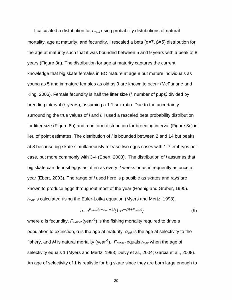
I calculated a distribution for rmax using probability distributions of natural

mortality, age at maturity, and fecundity. I rescaled a beta (α=7, β=5) distribution for

the age at maturity such that it was bounded between 5 and 9 years with a peak of 8

years (Figure 8a). The distribution for age at maturity captures the current

knowledge that big skate females in BC mature at age 8 but mature individuals as

young as 5 and immature females as old as 9 are known to occur (McFarlane and

King, 2006). Female fecundity is half the litter size (l, number of pups) divided by

breeding interval (i, years), assuming a 1:1 sex ratio. Due to the uncertainty

surrounding the true values of l and i, I used a rescaled beta probability distribution

for litter size (Figure 8b) and a uniform distribution for breeding interval (Figure 8c) in

lieu of point estimates. The distribution of l is bounded between 2 and 14 but peaks

at 8 because big skate simultaneously release two eggs cases with 1-7 embryos per

case, but more commonly with 3-4 (Ebert, 2003). The distribution of i assumes that

big skate can deposit eggs as often as every 2 weeks or as infrequently as once a

year (Ebert, 2003). The range of i used here is plausible as skates and rays are

known to produce eggs throughout most of the year (Hoenig and Gruber, 1990).

rmax is calculated using the Euler-Lotka equation (Myers and Mertz, 1998),

b= eFextinct 𝑎−𝛼𝑠𝑒𝑙 +1 (1-e—(𝑀+Fextinct)) (9)

where b is fecundity, Fextinct (year-1) is the fishing mortality required to drive a

population to extinction, α is the age at maturity, αsel is the age at selectivity to the

fishery, and M is natural mortality (year-1). Fextinct equals rmax when the age of

selectivity equals 1 (Myers and Mertz, 1998; Dulvy et al., 2004; Garcia et al., 2008).

An age of selectivity of 1 is realistic for big skate since they are born large enough to

21

be caught through trawl fisheries. I generated a distribution of rmax, by iteratively

solving Eq. 9 for Fextinct using unique combinations of α, b, and M in order to create

a prior probability distribution for the intrinsic growth rate, r, of the Graham-Schaefer

model. I tested the sensitivity of rmax to varying ages of selectivity to determine how

rmax would change if my assumption regarding age of selectivity was

underestimated.

Figure 8. Density distributions for age at maturity (years, a), litter size (number of pups, b), and breeding interval (years, c) used in the calculation of rmax.

2.6 Abundance and Management Parameter Estimation using BDMs

I developed prior probability distributions for the three Graham-Schaefer BDM

parameters: intrinsic growth rate (r), carrying capacity (K), and depletion which

estimates biomass at the start of the fishery as a proportion of K (Punt, 1990). Both

big skate stocks may have been at some fraction of K in 1996 because the

groundfish fishery began around 1954, and although not targeted, big skate landings

and discards may have occurred. The prior for r, aimed to match the distribution of

22

rmax, was best represented by a rescaled beta (α=3, β=15) distribution bounded

between 0.25-0.90 year-1(Eq. 10). The prior for K was a rescaled beta (α=1.15,

β=1.15) distributed between 1,000 and 10 million tonnes (Eq. 11). The wide, slightly

informative distribution for K attempted to give the model flexibility to find the most

probable value given the data. Depletion was uniformly distributed between 0 and 1

(Eq. 12).

p( 𝑟−0.25

0.90−0.25 ) ~ beta(α =3, β=15) (10)

p( 𝐾−1000

1e7−1000 ) ~ beta(α =1.15, β=1.15 ) (11)

p(depletion) ~ beta( α= 1, β=1) (12)

Each stock’s BDM fit the indices of population abundance by applying an

observation error estimator that assumed all error was present in the relationship

between stock abundance and the index of abundance (Polachek et al., 1993;

Hayes et al., 2009). The equation used to calculate the predicted index of

abundance is,

Ij,t= qjBt

(13)

where Ij,t is the value of the abundance for index j at time t, and q is the catchability

coefficient which scales the population size to the index j. The observation error

likelihood estimates the difference between the observed index of abundance and

the predicted index calculated through the model (Brodziak and Ishimura, 2011). A

value for σ was calculated for each index of abundance, j, using the equation,

σj = ( log Ij,t -log(Ij,t) ) 𝑡

1

𝑛 (14)

23

where Ij,t is the predicted index, calculated from the predicted q and predicted

biomass using Eq. 13, and n is the number of data points in the index time series. I

used the negative log-likelihood to determine the relative fit of the BDMs to the

catch, CPUE, and survey data. I calculated the negative log-likelihood for each index

of abundance assuming log-normal error.

-log L qj, r, K, depl, σj Ij,t = - log 1

𝐼𝑗 ,𝑡 2πσj2 +

1

2σj2 ( log(Ij,t)-log(Ij,t) )

2 (15)

The total negative log-likelihood was the sum of the negative log-likelihood of each

available index (Eq. 15) multiplied by the prior probability distributions of the three

Graham-Schaefer BDM parameters (Eqs. 10-12).

I used MCMC to sample from the posterior probability distributions of the three

BDM parameters. I drew 20 million iterations from each parameter’s MCMC chain,

with a burn-in of 2,000 and thinning by 1,000 for a total chain length of 19,998. I

checked MCMC diagnostics to verify chain convergence on the posterior distribution

of the parameters. I calculated probability distributions of management parameters

of interest (MSY, BMSY, and FMSY) using the posterior probability distributions of r and

K. I used each iteration of the MCMC chain to calculate the predicted big skate

population in each stock for the length of the time series along with 50, 80 and 90%

quantiles. Additionally, I used the median of the posterior distribution for the three

parameters to calculate predicted indices of abundance for each stock.

2.7 Depletion-Corrected Average Catch (DCAC)

The final component of the stock assessment was the use of depletion corrected

average catch analysis (DCAC) to calculate the potential yield (Ypot) and sustainable

24

yield (Ysust) of big skate in QCS and NHS (MacCall, 2009). Ypot is a conservative

estimate of MSY based on unfished biomass and natural mortality, and the Ysust is

the total removals that will maintain a stock at its current abundance given its

depletion over the catch time series. The calculations of Ypot and Ysust require a time

series of catch, an estimate of natural mortality (M), the ratio of FMSY to M (c), and

delta (Δ), the reduction in vulnerable biomass over the catch time series as a fraction

of the unfished biomass, B0. Larger positive values of Δ signify greater reductions to

stock size; negative values indicate a population that has increased over time

(Berkson et al., 2011). The first step to calculating Ysust requires the calculation of

Ypot. The equation used to calculate potential yield is,

Ypot= 0.4* c * M * Bo (16)

The term, c*M replaces the assumption that FMSY = M since studies have found that

this assumption may actually overestimate the fishing mortality a stock can

withstand (MacCall, 2009). I used the posterior distribution of FMSY calculated from

the BDM in lieu of c*M. Additionally, I used the posterior probability distribution of K

from the BDM component as Bo. Therefore, the equation I used to calculate Ypot is,

Ypot= 0.4* FMSY * K (17)

I used the posterior probability distributions of FMSY and K to calculate Ypot in order to

capture the uncertainty surrounding the true values of K and FMSY. Ypot is a

conservative estimate of MSY because according to Equation 17, BMSY is equal to

40% of K as opposed to 50% of K assumed in the logistic Graham-Schaefer model.

Ultimately, I used DCAC to determine the sustainable yield (Ysust) that can be

removed from the stock while maintaining its current abundance. The sustainable

25

yield takes into account a “windfall” ratio which represents the reduction of biomass

from B0 to BMSY. The equation for the sustainable yield is,

Ysust = C

n+W

Ypot

(18)

where C are the catches in the time series, n is the number of years in the catch

time series, and the ratio of W/Ypot (= Δ/0.4*FMSY) expresses the windfall relative to a

single year of potential yield. If no change in abundance occurred (i.e., Δ=0), the

equation for Ysust equals the average catch. If stock abundance increased, Δ and the

ratio W /Ypot are negative and Ysust is larger than average historical catches (McCall,

2009). Δ is calculated using the equation,

Δ= BFYR – BLYR / Bo (19)

where BFYR is the biomass in the first year of the time series, BLYR is the biomass in

the last year of the time series, and B0 is the unfished biomass (MacCall, 2009). I

used the predicted first and last year biomass from each stock’s BDM to calculate

the difference in biomass for each stock over the time series. I also used the

posterior probability distribution of K from the BDMs as the unfished biomass to

calculate a posterior distribution of Δ. According to the BDM predictions of first and

last year biomass and K, the 95% quantile of Δ for QCS was -0.65 - -0.01 from

1996-2010 and -0.89-0.0003 for NHS from 1984-2010. I drew random values of Δ

directly from the posterior estimates for each stock. The 95% quantiles of Δ for both

stocks are negative values thereby predicting that both stocks have increased over

their respective catch time series. However, the full ranges of Δ for both stocks

include zero (i.e., same biomass at first and last year) and positive estimates (i.e.,

decreasing biomass over the time series). The estimates of Ysust predicted by my

26

assumed range of Δs consider the uncertainty contained in BDM outputs. I

interpreted the estimated Ysust values given the stock abundance estimated by each

stock’s BDM.

27

3: RESULTS

3.1 Bayesian Approach to Estimate rmax from a Growth Curve

The posterior probability distributions of the von Bertalanffy growth

function (VBGF) parameters suggest that the data contained little information to

improve estimates of the asymptotic length, L∞ , but greatly improved estimates of

the growth rate, k, and age when length equals zero, t0. The observed female

length-at-age data contained some information regarding the most likely value of

L∞ as shown by the slight difference between the shape of the prior and posterior

probability distributions (Figure 9). A complete overlap between the prior and

posterior probability distributions would indicate that the data did not provide any

additional information to shape the posterior distribution. The skewed posterior

distributions of k and t0 are evidence that the data informed the shape of those

posterior distributions since the prior distributions used for both parameters were

flat (Figures 10 and 11). However, the inverse correlation that exists between L∞

and k may be a factor in the highly skewed shape of the k posterior. The

estimates of the mode of the L∞, k, and t0 posterior distributions equalled 2177

mm, 0.007 year-1, and -0.021 years, respectively. The median estimates of the

posterior distributions (L∞ = 2647 mm, k =0.044 year-1 and t0=-0.094 years)

consistently underestimate predicted lengths-at-age (Figure 12). Percentiles,

means, and standard deviations of the three VBGF parameter posterior values

are shown in Table 1.

28

The posterior distributions of L∞ and k produced a wide distribution of natural

mortality, M, whereas the distribution of population productivity, rmax, based on life

history parameters was highly informative. M ranged from 0.00035-0.347 year-1 with

a mode equal to 0.007 year-1(Figure 13). The skewed shape of the M distribution

may be due to the skewed shape of the k posterior used in its calculation. rmax

exhibited a tight distribution around the mode of 0.356 year-1 and ranged from 0.223-

0.772 year-1 (Figure 14).The shape of the distribution for rmax closely matches the

distributions of age at maturity and litter size used in its calculation. Table 2 shows

the 2.5, 25, 50, 75 and 97.5% quantiles, mean, and standard deviation of M and rmax.

The sensitivity analysis on the age of selectivity assumption shows that increasing

the age of selectivity while holding all other parameters constant increases the mean

and standard deviation of rmax (Figure 15).

Figure 9. Prior (dashed line) and posterior (solid line) probability distributions for

L∞ of the VBGF.

29

Figure 10. Prior (dashed line) and posterior (solid line) probability distributions of k, the growth rate of the VBGF.

Figure 11. Prior (dashed line) and posterior (solid line) probability distributions for t0 of the VBGF.

30

Figure 12. Observed (empty circles) versus predicted (solid line) length-at-age data for female big skate calculated using the median estimates from L∞, k, and t0 posterior distributions.

Figure 13. Density plot of annual natural mortality, M, calculated using Pauly’s (1980) equation (Eq. 8).

31

Figure 14. Density plot of rmax calculated by iteratively solving Eq. 11 using natural mortality, age at maturity, fecundity, and age of selectivity.

Figure 15. Probability distribution of rmax under different ages of selectivity (years)

to the fishery.

32

Table 1.Statistics from the posterior distributions of the three VBGF parameters sampled through MCMC .

Parameter 2.50% 25% Median 75% 97.50% Mean SD

L∞(mm) 2041 2331 2660 3023 3433 2687 413

k 0.00 0.01 0.04 0.09 0.26 0.06 0.07

t0 (years) -2.48 -0.49 -0.04 0.00 0.00 -0.40 0.68

Table 2.Statistics from the probability distributions of natural mortality, M, and rmax.

Parameter 2.50% 25% Median 75% 97.50% Mean SD

M (year-1) 0.001 0.016 0.038 0.068 0.149 0.047 0.040

rmax(year-1) 0.288 0.347 0.391 0.457 0.618 0.409 0.085

3.2 Management Parameter and Abundance Estimation Using BDMs

The highly informative prior probability distribution for the intrinsic growth

rate, r, influenced the posterior probability distributions for all three parameters of

the Graham-Schaefer biomass dynamics model. For both stocks, the prior and

posterior probability distributions completely overlapped signifying a lack of

information in the observed data (i.e., total catch, trawl landings CPUE, and

research survey data) regarding the true value of r (Figure 16). The lack of

contrast in the data set for each stock produced similar modes for the posterior

probability values of r equal to 0.366 year-1 and at 0.359 year-1 for QCS and NHS,

respectively. The modes of the posterior of r from each stock are almost equal to

the peak rmax (0.356 year-1) used to define the prior probability distribution of r,

further evidence that the observed data did not update the posterior distribution.

The posterior distributions of the carrying capacity, K, for both stocks were highly

skewed towards higher abundances, likely a result of the inverse relationship

33

between r and K (Figure 17). The modes of the posterior probability estimates of

K occurred at approximately 202,000 tonnes for QCS and 159,000 tonnes for

NHS. The mode of the depletion posterior distribution for QCS and NHS signified

that at the start of the targeted fishery in 1996 the stocks were at 72% and 78%

of K, respectively (Figure 18). The depletion results suggest that non-targeted big

skate mortality induced through other fisheries prior to 1996 is a possibility. The

median estimates of r, K, and depletion occurred at 0.385 year-1, 698,000 tonnes,

and 68% for QCS and 0.391 year-1, 501,000 tonnes, and 62% for NHS.

Quantiles, means, and standard deviations for the three BDM parameters for

each stock are shown in Table 3 and 4 for QCS and NHS, respectively.

Posterior distributions of MSY and BMSY exhibited high uncertainty

whereas FMSY was highly informative. The mode of the posterior for MSY for QCS

was higher than that for NHS, 21,800 tonnes versus 16,200 tonnes, respectively

(Figure 19). BMSY is directly related to K; therefore, the posterior distributions and

modes of BMSY in each stock exactly match that of K, except the values are

halved (Figure 20). The long tails present in the MSY and BMSY posterior

distributions are due to the highly skewed posterior for K because it factors into

both management parameter calculations (MSY=r*k/4 and BMSY=K/2) . Posterior

distributions for FMSY in each stock are directly related to the posterior

distributions for r and as a result also exhibit tight distributions about their modes

(Figure 21). Quantiles, means, and standard deviations for the three

management parameters are shown in Table 5 and 6 for QCS and NHS,

respectively.

34

Both QCS and NHS stocks had median predicted population abundances

at their carrying capacities. It is unlikely that the stocks are currently overfished

(as of 2010) as the median estimated population size is well above the estimated

BMSY. The median predicted population biomass for QCS started at 474,000

tonnes in 1996 and slowly increased to its final predicted biomass of 698,000

tonnes. For NHS the predicted population biomass was 313,000 tonnes in 1984

and stabilized at its final predicted biomass of 501,000 tonnes (Figure 22). The

predicted indices for QCS increased and then levelled off through the available

data points. The fit predicted by the BDM concerning the QCS stock results from

the lack of a trend in the later part of the CPUE time series and the contrasting

trends seen in the two fishery-independent indices of abundance (Figure 23).

Similarly, the CPUE time series and the Hecate Strait Multispecies survey for the

NHS stock was highly variable and showed little trend; hence, the model fit a

horizontal line through the later part of the time series (Figure 24).

35

Figure 16. Prior (solid line) and posterior (dashed line) probability distributions for the intrinsic growth rate for QCS (left) and NHS (right).

36

Figure 17. Prior (solid line) and posterior (dashed line) probability distributions

of the carrying capacity, K, for QCS (left) and NHS (right). X-axes were truncated to show shape of posterior at lower abundances as the posterior distribution did not change at abundances larger than 6,000,000 tonnes.

Figure 18. Prior (solid line) and posterior (dashed line) probability distributions for the depletion parameter of the Graham-Schaefer biomass dynamics model for QCS (left) and NHS (right).

37

Figure 19. MSY posterior probability distribution for QCS (solid line) and NHS

(dashed line) stocks measured in 1,000s of tonnes.

Figure 20. Posterior distribution of the biomass that sustains MSY, BMSY (tonnes), for QCS (solid line) and NHS (dashed line).

38

Figure 21. Posterior distribution of the instantaneous fishing mortality that results

in MSY, FMSY, for QCS (solid line) and NHS (dashed line) stocks.

Figure 22. The log predicted big skate population abundance in QCS (left) from 1996-2010 and NHS (right) from 1984-2010. The light grey is the 90% quantile, medium grey is the 80% quantile, dark grey is the 50% quantile and the solid black line is the median predicted population biomass.

39

Figure 23. Observed and predicted indices of abundance for the QCS stock of

big skate calculated using the median of the posterior distribution of the three Graham-Schaefer parameters. Fishery CPUE is shown on the left figure, QCS Synoptic Survey in the middle, and QCS Shrimp Survey on the right.

Figure 24. Observed and predicted indices of abundance for the NHS stock of big skate calculated using the median of the posterior distribution of the three Graham-Schaefer parameters. Fishery CPUE is shown on the left and the Hecate Strait Multispecies Survey on the right.

40

Table 3. Statistics from the posterior distribution of the three parameters of the Graham-Schaefer biomass dynamics model for Queen Charlotte Sound.

Parameter 2.50% 25% Median 75% 97.50% Mean SD

r (year-1) 0.285 0.342 0.385 0.441 0.579 0.397 0.076

K (tonnes) 10,963 129,080 698,266 2,718,540 8,222,520 1,836,096 2,379,094

depletion 0.332 0.542 0.680 0.824 0.980 0.678 0.181

Table 4. Statistics from the posterior distribution of the three parameters of the Graham-Schaefer biomass dynamics model for North Hecate Strait.

Parameter 2.50% 25% Median 75% 97.50% Mean SD

r (year-1) 0.283 0.343 0.391 0.450 0.578 0.402 0.077

K (tonnes) 6,594 76,652 501,174 2,385,481 8,587,588 1,650,477 2,340,178

depletion 0.091 0.399 0.624 0.808 0.980 0.597 0.256

Table 5. Statistics for the management parameters calculated using the posterior distributions of the three parameters of the Graham-Schaefer biomass dynamics model for Queen Charlotte Sound.

Management Target 2.50% 25% Median 75% 97.50% Mean SD

MSY (tonnes) 1,082 12,426 67,706 264,363 822,354 181,187 239,500

Bmsy (tonnes) 5,481 64,540 349,133 1,359,270 4,111,260 918,048 1,189,547

Fmsy 0.142 0.171 0.192 0.220 0.290 0.198 0.037

Table 6. Statistics for the management parameters calculated using the posterior distributions of the three parameters of the Graham-Schaefer biomass dynamics model for North Hecate Strait.

Management Target 2.50% 25% Median 75% 97.50% Mean SD

MSY (tonnes) 695 7,349 49,141 231,397 871,076 166,095 242,348

Bmsy (tonnes) 3,297 38,326 250,587 1,192,740 4,293,794 825,238 1,170,089

Fmsy 0.141 0.171 0.196 0.225 0.289 0.201 0.039

41

3.3 Depletion-Corrected Average Catch Analysis

DCAC estimates of potential yield (Ypot) for each stock were lower than the

MSY values estimated using the BDMs due to DCAC’s assumption of BMSY

occurring at 40% of B0 rather than 50% of B0. Resulting estimates of sustainable

yield (Ysust) were significantly lower than both the Ypot and MSY because both

stocks are estimated to be well above BMSY. If the stocks were at BMSY then they

would be able to sustain removals equal to Ypot; the mode of the Ypot posteriors

were estimated at 17,500 tonnes and 13, 000 tonnes for QCS and NHS,

respectively (Figure 25). According to the mode the of Ysust posteriors, QCS and

NHS stocks can sustain removals of 370 and 330 tonnes, respectively, without

changing the current estimated stock size (Figure 26). The current TAC on NHS,

equal to 567 tonnes, is lower than the maximum Ysust predicted by DCAC

(approximately 850 tonnes). Given the assumed range of Δ values, the range of

predicted Ysust for QCS was 300-2,400 tonnes and 225-850 tonnes for NHS. The

lower Ysust values for NHS compared to QCS may be a result of my zero catch

assumption from 1984-1995 for NHS. Also, lower Ysust values for NHS may be

due to the higher, positive Δ values predicted by the BDM for NHS (0.66 versus

0.11 for QCS). The relatively low Ysust values occur because the current predicted

abundance in each stock is near or at carrying capacity and thus experiencing

strong effects of density-dependence. Tables 7 and 8 show the 2.5, 25, 50, 75,

and 97.5% quantiles, mean, and standard deviation for Ypot and Ysust,

respectively..

42

Figure 25. Potential yield (Ypot) (solid line) calculated through DCAC compared to

MSY (dashed line) estimated from the Graham-Schaefer BDM for QCS (left) and NHS (right).

Figure 26. Sustainable yield (Ysust) distribution calculated using DCAC for the

QCS (left) and NHS (right) stocks.

43

Table 7.Statistics for the potential and sustainable yield distributions for the QCS stock of big skate calculated using DCAC methods.

Management Target 2.50% 25% Median 75% 97.50% Mean SD

Ypot 866 9,940 54,165 211,490 657,883 144,950 191,600

Ysust 327 382 442 533 865 480 154

Table 8.Statistics for the potential and sustainable yield distributions for the NHS stock of big skate calculated using DCAC methods.

Management Target 2.50% 25% Median 75% 97.50% Mean SD

Ypot 843 10,366 54,031 215,090 685,603 147,598 196,598

Ysust 300 325 359 411 568 379 73

3.4 Sensitivity Analyses on Discard Mortality Rate

The 0 and 100% discard mortality rates mainly affected the output

produced by DCAC. The DCAC sustainable yield increased for both stocks with

an increasing discard mortality rate (Tables 9 and 10). Sustainable yield

increased with increasing discard mortality rate because the total catch increases

when the model assumes more skate are dead post-capture. A higher historical

total catch increases the numerator in the sustainable yield equation thus

producing a larger sustainable yield. The QCS stock showed increasing K, MSY,

and BMSY with increasing discard mortality rates but trends for NHS were less

clear. Discard mortality rates did not affect the overall shape of the parameter

posterior distributions likely because discards were low relative to overall catch

(Appendix I and II).

44

Table 9. Modes of posterior probability distributions for QCS under the three discard mortality rate scenarios.

0% 50% 100%

r (year-1) 0.374 0.366 0.367

K (tonnes) 190,006 202,184 214,879

depletion 0.716 0.720 0.597

MSY (tonnes) 19,579 21,831 22,338

Bmsy (tonnes) 95,003 101,092 107,439

Fmsy 0.187 0.183 0.184

Ypot 15,663 17,464 17,871

Ysust 346 365 388

Table 10.Modes of posterior probability distributions for NHS under the three discard mortality rate scenarios.

0% 50% 100%

r (year-1) 0.367 0.359 0.361

K (tonnes) 136,358 158,603 172,482

depletion 0.743 0.789 0.749

MSY (tonnes) 14,732 16,196 15,655

Bmsy (tonnes) 68,179 79,302 86,241

Fmsy 0.184 0.179 0.180

Ypot 11,786 12,957 12,524

Ysust 290 325 365

45

4: DISCUSSION

The biomass dynamics models (BDMs) for Queen Charlotte Sound (QCS)

and North Hecate Strait (NHS) predict both stocks to be stable at their respective

carrying capacities given the available data. However, the population abundance

estimates and their relationship to carrying capacity are uncertain since CPUE

and survey indices lacked the variation needed to reliably fit a BDM. The BDMs

predict maximum sustainable yields (MSY) of 21,800 and 16,200 tonnes.

Depletion-corrected average catch (DCAC) analysis predicts that if the

population is to remain at its current abundance, 370 and 330 tonnes may be

removed sustainably (Ysust) from QCS and NHS, respectively. If the stocks were

at the biomass that supports MSY (BMSY) they could support removals equal to

MSY, or, if managers wish to be more conservative, equal to the potential yield

calculated by DCAC (16,500 and 13,000 tonnes for QCS and NHS). However,

because the models predict both stocks to be at carrying capacity they are not as

productive as they would be if at BMSY. The following sections discuss how the

uncertainty in available life history and fishery data affect model outcomes. I

follow with applications of my stock assessment results to potential management

objectives and summarize with conclusions.

46

4.1 Bayesian Approach to Estimate rmax from a Growth Curve

The female length-at-age data used to fit the von Bertalanffy growth

function (VBGF) created difficulties for parameter estimation. The available

length-at-age data did not reach an asymptote within the observed range of

lengths. Consequently, the data contained little information on the true value of

L∞ as evidenced by the similar shapes of the prior and posterior probability

distributions. The mean and median posterior estimates of L∞ were higher than

the estimated L∞ for female big skate in the Gulf of Alaska (GOA) (Gburski et al.,

2007). The difference in L∞ is not surprising given that no big skates larger than

1780 mm were observed in the GOA study whereas skates as large as 2040 mm

have been observed in BC. The median of the posterior distribution of k, the

growth rate of the VBGF, was approximately half the k estimated for GOA big

skate, 0.0796 year-1(Gburski et al., 2007). Estimates of k for big skate calculated

using life history invariant equations equalled 0.10-0.14 year-1 (Benson et al.,

2001). The re-capture and ageing of larger (and older) female big skate would

greatly improve the data set used to fit the VBGF and subsequent parameter

estimations.

Natural mortality (M) is vital for inputs to stock assessments but it is also

one of the most difficult parameters to calculate directly, hence it is usually

calculated indirectly from a growth curve using life history invariant theory (Hewitt

and Hoenig, 2005). The width of L∞ and k posterior distributions resulted in a

wide range of possible M values. However, the resulting distribution of M

accounts for uncertainty in both the life history parameters and model coefficients

47

used in its calculation. My research produced model estimates of M similar to

those of the roughskin skate (Dipturus trachyderma) which grows to similar sizes

as the big skate and has an estimated mean M between 0.089-0.184 year-1

(Quiroz et al., 2010). Researchers estimate maximum age of big skate to be

approximately 26 years which results in a natural mortality of 1/26, or 0.038 year-

1, based on life history theory (King and McFarlane, 2010). Big skate natural

mortality estimated from a predictive equation based on data from numerous fish

stocks is larger than the median and mean estimated in my assessment (0.162

year-1 versus 0.037 and 0.047 year-1; Hoenig, 1983; Hewitt and Hoenig, 2005).

However, the oldest observed skate likely underestimates the true maximum age

and the larger estimate based on the predictive equation is still within the range

of possible M values calculated in my model. I recommend an alternate method

of calculating natural morality (e.g., Hoenig and Hewitt, 2005) given the

uncertainty present in the estimates of L∞ and k, until more data becomes

available.

The probability distribution of rmax incorporated all possible sources of

uncertainty in the form of probability distributions for the life history parameters

used in its calculation: asymptotic maximum length (L∞), growth rate (k), age at

maturity (α), breeding interval (i), and litter size (l). A previous estimate of

potential rate of population increase (r’=0.26 year-1, Benson et al., 2001),

calculated using female maximum length (Lmax= 1680 mm), is smaller than the

mean rmax estimated in this research. However, the rmax calculated in my research

considered other life history parameters, such as litter size and breeding interval,

48

which may attribute to the larger mean rmax (Benson et al., 2001; Frisk et al.,

2001). Through the sensitivity analysis of age at selectivity on rmax, I found that as

the age of selectivity to the fishery approaches the age of maturation, the Euler-

Lotka model predicts a larger mean and range for rmax (Myers and Mertz, 1998).

Therefore, if the actual age of selectivity of big skate is larger than one, the

resulting distribution of rmax may not be as informative as the distribution

produced in the current assessment. In order to facilitate the calculation of

selectivity curves for big skate, onboard observers should collect length data on

trawl tows that target big skate whenever possible.

4.2 Uncertainty in Management Parameter and Abundance Estimation using BDMs and DCAC

Posterior distributions for r, K, and depletion for QCS and NHS were

highly dependent on the informative prior probability distribution used for r. Due

to the lack of variation in the CPUE and survey data, the prior probability

distribution of r outweighs the likelihood of the data resulting in a posterior

distribution for r that identically matches its prior distribution. The informative prior

for r influences the posterior distribution for K since these two parameters are

inversely correlated (Hilborn and Walters, 1992). In order to get reliable

estimates of K, fishery data needs to have contrast. Ideally, data should be

collected from when the population is near K (i.e., pre-exploitation), when it has

been fished to low abundances, and then when it is allowed to recover.

Furthermore, the informative prior for r also indirectly affects the posterior

distribution of depletion since it is calculated jointly with r and K.

49

The extent of uncertainty in estimates of MSY, BMSY and FMSY are directly

related to the uncertainty in the estimates of r and K. The high uncertainty in the

estimates of MSY is due in part to the high uncertainty in K while estimates of

BMSY are entirely dependent on the uncertainty of the K posterior. The tight

distribution of the FMSY posteriors are a function of the informative priors and tight

posterior distributions for r. For elasmobranchs, MSY generally ranges between

4.5 and 7.5% of the unexploited biomass (Anderson, 1990). The MSY was

estimated between 6.5 and 7.6% of the unexploited biomass in a multispecies

ray fishery in the South Atlantic (Agnew et al., 2000). I found the mode of the

MSY posterior to be approximately 10% of the mode of the K posterior in both

QCS and NHS (21,800/202,000 tonnes for QCS and 16,200/159,000 tonnes for

NHS). It is likely that creating an informative prior for K, possibly by using density

estimates for big skate and area swept data from research surveys, would

narrow the range of possible MSY and BMSY values.

The median predicted population size and predicted indices of abundance

of big skate in each stock were stable during the later part of the time series. The

wide range of predicted population sizes results from the skewed K posterior

distribution. As previously mentioned, creating an informative prior for K could

generate a narrower range of predicted population abundances. The model

output suggests that the catch taken from 1996-2010 did not have a significant

effect on the population dynamics of big skate in either stock. The best fit to the

multiple indices of abundance used in my assessment was a relatively horizontal

line through the later data points in the time series and was likely due to the

50

variability and lack of contrast in the data. It is unknown if the lack of trends

observed in the data are representative of the true population abundance.

The DCAC potential yield is a conservative estimate of MSY while the

DCAC sustainable yield calculates the yield that can be removed from the stock

while maintaining the stock at its current abundance (MacCall, 2009). The

potential yield was slightly lower than the MSY estimated from the BDMs

because the potential yield equation assumes BMSY occurs at 40% of B0 whereas

the Graham-Schaefer assumes BMSY occurs at 50% of B0. I recommend using the

potential yield in lieu of MSY as BMSY for elasmobranchs is believed to occur

between 35-48% of unfished biomass (Anderson, 1990). The DCAC sustainable

yield is significantly lower than the potential yield and MSY because both stocks

are estimated to be at carrying capacity. A stock at carrying capacity is not as

productive as a stock below carrying capacity due to the strong effects of density-

dependence resulting in low birth rates relative to death rates. The BDMs

predicted an increase in both stock’s biomass since the beginning of their

respective time series; hence, most of the depletion (Δ) values assumed were

negative and the resulting modal sustainable yields predicted (370 and 330

tonnes for QCS and NHS) are larger than the average of historic catches (323

and 301 tonnes for QCS and NHS).

4.3 Management Applications

A harvest strategy for the big skate fishery in British Columbia requires

clear management objectives from DFO. There is currently a total allowable

catch (TAC) of 567 tonnes in NHS, but there is no TAC for big skate in QCS

51

(DFO, 2011). The TAC encompasses both landings and estimated discards in

the trawl sector of the fishery (DFO, 2011). In accordance with DFO’s goal to

adhere to the precautionary approach, all management advice needs to account

for uncertainty while taking action to avoid harm to stocks and the ecosystem

(DFO, 2006). DFO incorporates the precautionary approach into their stock

assessments by defining three zones that describe stock status: healthy,

cautious, and critical (DFO, 2006). The lower limit reference point (LRP) divides

the critical zone from the cautious zone (DFO, 2006). Below the LRP, the stock is

in the critical zone, the removal rate (usually expressed in terms of fishing

mortality) approaches zero, and efforts to promote stock re-building are initiated.

The upper stock reference (USR) divides the cautious zone from the healthy

zone (DFO, 2006). Below the USR, the stock is in the cautious zone and the

removal rate from the stock is reduced accordingly in order to avoid reaching the

LRP. Above the USR, the stock is in the healthy zone. Therefore, a target

reference point (TRP), a desirable target for management, should be above the

USR to maintain the stock in the healthy zone. Ultimately, the harvest rate

chosen depends on the zone in which the stock lies. For example, if the stock is

in the cautious zone harvest rates are set so that the stock rebuilds into the

healthy zone (DFO, 2006). DFO’s Sustainable Fishery Framework states that

DFO’s goal is to keep stocks in the healthy zone and out of the critical zone

(DFO, 2011). I will outline two potential DFO management goals, their

accompanying management advice based on the results of this assessment, and

discuss data collection routines to improve future management advice.

52

The first potential DFO management goal may be to maintain big skate

abundance at current levels. I estimated that both stocks are near or at carrying

capacity, thus experiencing relatively low productivity due to density dependence.

Hence, the only way to maintain current stock size and the resultant low

productivity is through relatively low removals. Big skate catch increased by

245% since 2008 in QCS and by 72% since 2007 in NHS, yet both stocks

continue to be near their respective carrying capacities. According to my

assessment, both big skate stocks have remained relatively stable even with the

current catches and the relatively high catch taken in both stocks in 2003. My

study shows that the catches experienced during the time series available had

little effect on big skate population dynamics. If big skate catches from QCS and

NHS remain within the range of past catches then DFO will be able to maintain

the current big skate abundance without having to establish a TAC. DFO should

continue to monitor catches, continue to track population trends through fishery-

independent surveys, and reassess population status in a few years or earlier if

there is a dramatically large increase in catches.

DFO fishery managers may be interested in more conservative skate

management considering the declines of skate species in global fisheries

(Brander, 1981; Casey and Myers, 1998; Walker and Hislop, 1998; Dulvy et al.,

2000) coupled with the possibility of increased skate catch in BC to supply global

demand. To do this, managers can set a TAC in QCS equal to the largest

predicted DCAC sustainable yield (2,400 tonnes) and in NHS equal to the

highest catch from the time series (approximately 1,000 tonnes). I do not

53

recommend managers use the DCAC sustainable yield predicted for NHS

because my assumption of zero catch from 1984-1995 had a significant effect on

the calculated average catch. Average catch from 1984-2010 is 301 tonnes

(=8,140 tonnes/27 years) but average catch from 1996-2010 is 542 tonnes

(=8,140 tonnes/15 years). Had I only used catch data from 1996-2010 or

assumed non-zero catch from 1984-1995, the resulting sustainable yield

estimates would be larger than those presented in this assessment. Zero big

skate catch from 1984-1995 is unlikely because, although not targeted prior to

1996, they were likely caught and discarded in trawl fisheries (Benson et al.,

2001). Once the TAC for big skate is met in either stock, fishing for big skate

would cease in that location. Since big skate are caught alongside other

commercially important species, such as Pacific cod, setting a TAC for big skate

would potentially impact fisheries for other species.

Like most tactics used to regulate fisheries, TACs have advantages and

disadvantages. An output control, such as a TAC, has the benefit of regulating

how much catch is taken as opposed to using an input control, such as fixed

season length, which cannot control for effort. Additionally, input controls (e.g., a

limit on the number of trips taken) are harder to decrease in a fishery and can

lead to increases in effort through other mechanisms such as increases in fishing

power through technical means (Beddington et al., 2007). Two of the main

disadvantages of TACs are that they require a large amount of data and are

expensive to implement because of monitoring and enforcement (Hilborn and

Walters, 1992). However, monitoring and enforcement costs are already borne

54

by DFO and the fishery so the marginal cost will be small compared to the

benefits of monitoring catch and a lower risk of moving into an undesirable stock

status zone. Another important disadvantage in using TACs is that they assume

stock size is well known. If stock size is over-estimated, the TAC put in place

may actually be too high, driving the stock abundance down. The effect of over-

estimating a TAC will have prolonged effects on future stock sizes and catches

(Hilborn and Walters, 1992). Conversely, if the stock size is under-estimated, the

TAC will also be underestimated and managers will unknowingly forego potential

profit. Choosing a TAC for the big skate stocks may be difficult given the

information available.

DFO’s second potential management goal could be to maximize the

productivity and profitability of the big skate fishery. Given that my study

estimates both stocks to be at carrying capacity, each stock would first need to

be fished down to its BMSY, which under logistic growth assumptions is

approximately half a stock’s carrying capacity. Since big skate catches are driven

by market demand, establishing a higher TAC may not be enough to decrease

the stocks to BMSY. The established TAC in NHS does not seem to limit the

fishery as evidenced by the low catches relative to the 567 tonnes TAC

(excluding 2003). Additionally, catches in QCS have not exceeded 1,000 tonnes

even though there is no TAC present on big skate catch in that stock. Based on

the big skate catch trajectory it seems that there are other factors influencing

why, when, and how much fishers target and land big skate. Managers can

employ incentives, such as priority access to increased quota for other target

55

species, to motivate fishers to target and catch big skate. Once stocks are

reduced to BMSY they are more productive than a stock at carrying capacity and

can support removals equal to MSY. Managers can introduce a Limited Access

Program (LAP) to limit vessel numbers in order to avoid overcapitalization, thus

ensuring increased profits for those active in the fishery (Quigley, 2006).

Managers can use adaptive management and decision analysis to determine the

incentive program that is most likely to reduce big skate abundance and increase

profitability.

Adaptive management is an iterative process by which a management

regulation is enforced, the outcome is monitored, and the current management

regulation is updated using the knowledge gained (Lee, 1999). Adaptive

management treats policy decisions as large-scale experiments. These

experiments provide a way to learn about dynamic, complicated systems and can

potentially improve management (Walters, 2007). Decision analysis,

recommended for use in shark stock assessments (McAllister et al., 2001), could

be used by DFO managers to select an incentive program to motivate fishers to

reduce big skate abundance. A decision analysis would require the alternative

uncertain states of nature, the probability of each uncertain state occurring, and

decision tables to determine the probability of each outcome (McAllister et al.,

1994). For BC’s big skate fishery, the potential management decisions are

different incentive programs to get fishers to target big skate. The uncertain

states of nature are the r and K parameters from the biomass dynamics model,

which dictate predicted population size, the predicted response of the fishers to

56

the incentive program, and the catch resulting from the incentive program

chosen. The probabilities associated with each value of r and K can be taken

directly from the posterior probability distributions generated from the biomass

dynamics model used in this assessment. The predicted response of fishers to

an incentive program and the resulting catch can be determined by fisher

preference surveys and interviews as some incentives may be more attractive

than others. Incentives deemed more attractive by fishers may be more effective

at reducing the population to the desired abundance. Multiple outcomes are

possible from the decision analysis such as the time it would take to fish the

stock down to BMSY, the revenue generated from the catch level resulting from a

particular incentive program, and/or the cost of the incentive program. Managers

can apply the results from the decision analysis in an adaptive management

approach to one stock (the experimental unit) while keeping the other stock as a

control. The principal benefit of an adaptive management approach is the ability

to empirically reduce the uncertainty inherent in fisheries management by

undertaking experiments and updating existing knowledge (Botsford et al., 1997).

Adaptive management can be costly in terms of time and money when a suitable

solution is not found (Lee, 1999). However, adaptive management provides a

long-term plan and the opportunity to learn about system responses to

management as opposed to establishing a quota and monitoring outcomes.

Data collection and monitoring is an on-going and pivotal part of the

management process regardless of management objectives. Data collection and

monitoring can determine the efficacy of current management regulations. Data

57

collection in the form of a depletion experiment can determine if research surveys

(and fishery CPUE) are capturing true population trends (Hilborn and Walters,

1992). Additionally, depletion experiments in localized areas can give scientists

and managers an estimate of abundance (Hilborn and Walters, 1992). To do this,

I would recommend an experimental fishing-down of a portion of one stock while

using the other as a control. If a portion of the experimental stock is depleted,

one would expect to see a subsequent decrease in the CPUE and fishery-

independent survey indices conducted in that stock. Survey procedures should

measure relative abundance and use consistent gear and effort over time

(Hilborn and Walters, 1992). After five years, the survey can be used along with

fishery catches to determine initial and current stock sizes (Hilborn and Walters,

1992). Knowledge of current stock size can ensure that management regulations

do not jeopardize stock status (i.e., move it into the cautious or critical zones). As

onboard observers are already present on 100% of trawls in BC, length data on

commercially caught big skate can provide information on size-selectivity to the

fishery. Knowledge of size-selectivity is important because if fishers are targeting

older, mature skates they may be reducing the reproductive potential of the

population. Size-selectivity data could then be used to set minimum size limits on

skate catch, if necessary, to reduce the chance of recruitment overfishing.

58

5: CONCLUSIONS

The model output presented here suggests that the two big skate stocks

are unlikely to be overfished, as their estimated biomass is above the mode of

their estimated BMSY. If DFO’s management goal is to maintain the current level

of abundance in each stock, managers should monitor catches to ensure they

are within the range of catches taken from 1996-2010. A TAC is not necessary

since the historic catches do not seem to affect population dynamics according to

my model. If fishery managers wish to be conservative, a TAC could be set to

2,400 tonnes for QCS based on the maximum predicted DCAC sustainable yield

and 1,000 tonnes for NHS based on the highest catch from the time series

available. If DFO’s management goal is to increase the productivity and

profitability of the big skate fishery, I would recommend a fishing down of the

stocks to their BMSY. An adaptive management approach can be taken on one of

the two stocks to determine what incentive program motivates fishers to reduce

stock abundance to BMSY while also increasing profitability of the fishery. DFO

should continue to collect data through depletion experiments and monitor stock

status through trends in fishery-independent surveys. The research presented

here provides fishery managers with results that incorporate uncertainty and can

inform future management regulations for big skate in British Columbia.

59

LITERATURE CITED

Agnew, D.J., Nolan, C.P., Beddington, J.R., and Baranowski, R. 2000. Approaches to the assessment and management of multispecies skate and ray fisheries using the Falkland Islands fishery as an example. Canadian Journal of Fisheries and Aquatic Science, 57: 429-440.

Alverson, D.L., Freeberg, M.H., Murawski, S.A., and Pope, J.G. 1994. A global assessment of fisheries bycatch and discards. Food and Agriculture Organization Technical Paper,339. http://www.fao.org/DOCREP/003/T4890E/T4890E00.HTM

Anderson, E. D. 1990. Fishery models as applied to elasmobranch fisheries. Elasmobranchs as living resources: advances in the biology, ecology, systematics and the status of the fisheries. NOAA Technical Report NMFS, 90: 479-490.

Bayes, T. 1763. An essay towards solving a problem in the doctrine of chances. Philosophical Transactions of the Royal Society of London, 53: 370-418.

Beddington, J.R., and Kirkwood, G.P. 2005. Estimation of potential yield and stock status using life-history parameters. Philosophical Transactions of the Royal Society of London B, 360: 163-170.

Beddington, J.R., Agnew, D.J., and Clark, C.W. 2007. Current problems in the management of marine fisheries. Science, 316: 1713-1716.

Benson, A.J., McFarlane, G.A., and King, J.R. 2001. A phase "0" review of elasmobranch biology, fisheries, assessment and management. Canadian Science Advisory Secretariat Research Document 129.

Berkson, J., L. Barbieri,L., Cadrin,S., Cass-Calay, S.L., Crone, P., Dorn, M., Friess, C., Kobayashi, D., Miller,T.J., Patrick, W.S., Pautzke, S., Ralston, S., and Trianni, M. 2011. Calculating acceptable biological catch for stocks that have reliable catch data only (Only Reliable Catch Stocks – ORCS). NOAA Technical Memorandum NMFS-SEFSC-616, 56 pp.

Beverton, R. J. H., and Holt, S.J. 1959. A review of the life-spans and mortality rates of fish in nature and their relationship to growth and other physiological characteristics. CIBA Foundation Symposium-The Lifespan of Animals (Colloquia on Ageing),5: 142-180.

Botsford, L.W., Castilla, J.C., and Peterson, C.H. 1997. The management of fisheries and marine ecosystems. Science, 227: 509-515.

60

Brodziak, J., and Ishimura,G. 2011. Development of Bayesian production models for assessing the North Pacific swordfish population. Fisheries Science, 77: 23-34.

Charnov, E.L., Gillooly, J.F. 2004.Size and temperature in the evolution of fish life histories. Integrative and Comparative Biology, 44: 494–497.

Chromanski, E.M., Fargo, J., Workman, G.D., and Mathias, K. 2004. Multispecies trawl survey of Hecate Strait, F/V Viking Storm, June 10 - 28, 2002. Canadian Data Report of Fisheries and Aquatic Sciences, 1124.

Clarke, S. 2008. Toward species-specific catch and CPUE time series for sharks caught by the Japanese longline fishery in the Atlantic Ocean. Collective Volume of Scientific Papers, ICCAT, 62: 1477-1482.

Cooper, A.B., and Miller, T.J. 2007.Bayesian statistics and the estimation of nest-survival rates. Studies in Avian Biology, 34: 136-144.

Fisheries and Oceans Canada (DFO). 1999. Shrimp survey bulletin 99-03. http://www-ops2.pac.dfo-mpo.gc.ca/xnet/content/shellfish/shrimp/Surveys/9903_qcs.pdf.

DFO. 2000. Shrimp survey bulletin 00-04. http://www-ops2.pac.dfo-mpo.gc.ca/xnet/content/shellfish/shrimp/Surveys/0004_qcs.pdf.

DFO, 2006. A harvest strategy compliant with the precautionary approach. Canadian Science Advisory Secretariat, Science Advisory Report 2006/023. http://www.dfo-mpo.gc.ca/csas/Csas/status/2006/sar-as2006_023_e.pdf.

DFO, 2007. National plan of action for the conservation and management of sharks.http://www.dfo-mpo.gc.ca/npoa-pan/npoa-pan/npoa-sharks_e.pdf.

DFO, 2009. A fishery decision-making framework incorporating the precautionary approach. http://www.dfo-mpo.gc.ca/fm-gp/peches-fisheries/fish-ren-peche/sff-cpd/precaution-eng.htm.

DFO, 2011. Pacific Region Integrated Fisheries Management Plan, Groundfish, February 21, 2011 to February 20, 2013. Fisheries and Oceans Canada. http://www.pac.dfo-mpo.gc.ca/fm-gp/mplans/ground-fond_2012-13.pdf

Dick, A.J., and MacCall, A.D. 2010. Estimates of sustainable yield for 50 data-poor stocks in the Pacific coast groundfish fishery management plan. National Oceanic and Atmospheric Administration-Technical Memorandum-National Marine Fisheries Service-Southwest Fisheries Science Center-460.

Dulvy, N.K., Metcalfe, J.D., Glanville, J., Pawson, M.G., and Reynolds, J.D. 2000. Fishery stability, local extinctions and shifts in community structure in skates. Conservation Biology, 14: 283-293

61

Dulvy, N.K., Ellis, J.R., Goodwin, N.B., Grant, A., Reynolds, J.D., and Jennings, S. 2004. Methods of assessing extinction risk in marine fishes. Fish and Fisheries, 5: 255-276.

Dulvy, N.K., Baum, J.K., Clarke, S., Compagno,L.J.V., Cortes, E., Domingo,A., Fordham,S., Fowler,S., Francis, M.P., Gibson,C., Martinez, J., Musick, J.A., Soldo, A., Stevens, J.D., and Valenti, S. 2008. You can swim but you can’t hide: the global status and conservation of oceanic pelagic sharks and rays. Aquatic Conservation: Marine and Freshwater Ecosystems, 18: 459-482.

Dulvy, N.K., and Forrest, R.E. 2010. Life histories, population dynamics, and extinction risks in Chondrichthyans. In Sharks and their relatives II, 2ndedn, pp 639-680. Ed. by J.C. Carrier, J.A. Musick, and M.R. Heithaus. CRC Press, Boca Raton, FL. 736 pp.

Ebert, D.A. 2003. Sharks, rays, and chimaeras of California. University of California Press, Berkeley, California. 297 pp.

Ellison, A.M. 1996. An introduction to Bayesian inference for ecological research and environmental decision-making. Ecological Applications, 6: 1036-1046.

Enever, R., Catchpole, T.L., Ellis, J.R., and Grant, A. 2009. The survival of skates (Rajidae) caught in demersal trawlers fishing in UK waters. Fisheries Research, 97: 72-76.

FAO. 1999. International Plan of Action for the conservation and management of sharks. Food and Agriculture Organization of the United Nations, Rome, 8 pp.

FAO, 2012. The State of World Fisheries and Aquaculture. Rome. 209 pp.

Frisk, M.G., Miller, T. J., and Fogarty, M. J. 2001. Estimation and analysis of biological parameters in elasmobranch fishes: a comparative life history study. Canadian Journal of Fisheries and Aquatic Science, 58: 969-981.

Froese, R. and D. Pauly. Editors. 2011.FishBase.World Wide Web electronic publication. www.fishbase.org, version

Garcia, V.B., Lucifora, L.O., and Myers, R.A. 2008. The importance of habitat and life history to extinction risks in sharks, rays, skates and chimaeras. Proceedings of the Royal Society B, 275: 83-89.

Gburski, C.M., Gaichas, S.K., and Kimura, D.K. 2007. Age and growth of big skate (Raja binoculata) and longnose skate (Raja rhina) in the Gulf of Alaska. Environmental Biology of Fishes, 80: 337-349.

Gelman, A., Carlin, J.B., Stern, H.A. and Rubin, D.B. 2004. Bayesian data analysis. Chapman and Hall, Boca Raton. 668 pp.

62

Gertseva, V.V. 2009. The population dynamics of the longnose skate, Raja rhina, in the northeast Pacific Ocean. Fisheries Research, 95: 146-153.

Hayes, C.G., Jiao, Y., and Cortes, E. 2009. Stock assessment of scalloped hammerheads in the western North Atlantic Ocean and Gulf of Mexico. North American Journal of Fisheries Management, 29: 1406-1417.

Hewitt, D.A., and Hoenig, J.M. 2005. Comparison of two approaches for estimating natural mortality based on longevity. Fishery Bulletin, 103: 433-437.

Hilborn, R., and Walters, C.J. 1992. Quantitative Fisheries Stock Assessment: Choice, Dynamics and Uncertainty. Chapman & Hall, New York. 592 pp.

Hoenig, J.M. 1983. Empirical use of longevity data to estimate mortality rates. Fishery Bulletin, 82: 898–902.

Hoenig, J. M., and Gruber, S. H. 1990. Life-history patterns in the elasmobranchs: implications for fisheries management. In Elasmobranchs as Living Resources: Advances in the Biology, Ecology, Systematics, and the Status of the Fisheries. Proceedings of the Second United States–Japan Workshop East–West Center, Honolulu, Hawaii, 9–14 December 1987, pp. 1–16. Ed. by H. L. Pratt, S. H. Gruber, and T. Taniuchi. NOAA Technical Report NMFS, 90.518 pp.

Hoenig, J.M., Warren, W.G., and Stocker, M. 1994. Bayesian and related approaches to fitting surplus production models. Canadian Journal of Fisheries and Aquatic Science, 51: 1823-1831.

Jennings, S., Reynolds, J.D., and Mills, S.C. 1998. Life history correlates of responses to fisheries exploitation. Proceedings of the Royal Society B, 265: 333-339.

King, J.R., and McFarlane G.A. 2010. Movement patterns and growth estimates of big skate (Raja binoculata) based on tag-recapture data. Fisheries Research, 101: 50-59.

Laptikhovsky, V.V. 2004. Survival rates for rays discarded by the bottom trawl squid fishery off the Falkland Islands. Fishery Bulletin, 102: 757-759.

Lack, M., and Sant, G. 2009. Trends in global shark catch and recent developments in management. TRAFFIC International.

Lee, K. N. 1999. Appraising adaptive management. Conservation Ecology, 3: 3.

Link, W.A., Cam, E., Nichols, J.D., and Cooch, E.G. 2002. Of bugs and birds: Markov Chain Monte Carlo for hierarchical modelling in wildlife research. The Journal of Wildlife Management, 66: 277-291.

63

MacCall, A. D. 2009. Depletion-corrected average catch: a simple formula for estimating sustainable yields in data-poor situations. International Council for the Exploration of the Seas Journal of Marine Science, 66: 2267–2271.

Martin, A.D., and Quinn, K.M. MCMCpack: Markov chain Monte Carlo (MCMC) Package, 2005. URLhttp://mcmcpack.wustl.edu.R package version 0.6-3.

McAllister, M.K., Pikitch, E.K., Punt, A.E., and Hilborn, R. 1994. A Bayesian approach to stock assessment and harvest decisions using the sampling/importance resampling algorithm. Canadian Journal of Fisheries and Aquatic Science, 54: 2673-2687.

McAllister, M.K. and Kirkwood, G.P. 1998. Bayesian stock assessment: a review and example application using the logistic model. International Council for the Exploration of the Seas Journal of Marine Science, 55: 1031-1060.

McAllister, M.K., Pikitch, E.K., and Babcock, E.A. 2001.Using demographic methods to construct Bayesian priors for the intrinsic rate of increase in the Schaefer model and implications for stock rebuilding. Canadian Journal of Fisheries and Aquatic Science, 58:1871-1890.

McFarlane, G.A., and King, J.R., 2006. Age and growth of big skate (Raja binoculata) and longnose skate (Raja rhina) in British Columbia waters. Fisheries Research, 78: 169–178.

McQueen, D., and Ware, D. 2006. Handbook of physical, chemical, phytoplankton, and zooplankton data from Hecate Strait, Dixon Entrance, Goose Island Bank and Queen Charlotte Sound. Canadian Data Report of Fisheries and Aquatic Sciences, 1162.

Myers, R.A., and Mertz, G. 1998. The limits of exploitation: a precautionary approach. Ecological Applications, 8: S165-S169.

Pardo, S.A., Cooper, A.B., Carlson, J.K., Harrison, L.R., and Dulvy, N.K. 2010.Quantifying the known unknowns: the importance of accounting for uncertainty in elasmobranch demography. ICES CM 2010/E:24, 38 p.

Pauly, D. 1980. On the interrelationships between natural mortality, growth parameters, and mean environmental temperature in 175 fish stocks. Conseil International pour l'Exploration de la Mer, 39: 175-192.

Plummer, M., Best, N., Cowles, K., and Vines, K. 2006.CODA: convergence diagnostics and output analysis for MCMC. R News, 6:7-11.

Polachek, T., Hilborn, R., and Punt, A.E. 1993. Fitting surplus production models: comparing methods and measuring uncertainty. Canadian Journal of Fisheries and Aquatic Science, 50: 2597-2607.

Prager, M.H. 1994. A suite of extensions to a nonequilibrium surplus-production model. Fishery Bulletin, 92:374-389.

64

Punt, A. E. 1990. Is B1= K an appropriate assumption when applying an observation error production model estimator to catch–effort data? South African Journal of Marine Science, 9:249–259.

Punt, A.E., and Hilborn, R. 1997. Fisheries stock assessment and decision analysis: the Bayesian approach. Reviews in Fish Biology and Fisheries, 7: 35-63.

Quigley, Kate. 2006. Limited Access Privilege (LAP) programs and potential application to the south Atlantic snapper-grouper fishery. http://www.safmc.net/SocioEconomic/LimitedAccessPrivileges/tabid/486/Default.aspx

Quiroz, J. C., Wiff, R., and Caneco, B. 2010. Incorporating uncertainty into estimation of natural mortality 13 for two species of Rajidae fished in Chile. Fisheries Research, 102: 297-304.

R Development Core Team.2009. R: A language and environment for statistical computing. R 16 Foundation for Statistical Computing. Vienna, Austria. URL http://www.R-project.org.

Reynolds, J.D., Jennings, S., and Dulvy, N.K. 2001.Life histories of fishes and population responses to exploitation. In Conservation of Exploited Species, pp. 148-168.Ed. by J.D. Reynolds, G.M. Mace, K.H. Redford and J.G. Robinson. Cambridge University Press, Cambridge.548 pp.

Schaefer, M. B. 1954. Some aspects of the dynamics of populations important to the management of the commercial marine fisheries. Bulletin of the Inter-American Tropical Tuna Commission, 1:25–56.

Siegfried, K.I., and Sanso, B. 2006.Two Bayesian methods for estimating parameters of the von Bertalanffy growth equation. Environmental Biology of Fishes, 77: 301-308.

Stobutzki, I. C., Miller, M.J., Heales, D. S., and Brewer, D. T.2002. Sustainability of elasmobranchs caught as bycatch in a tropical prawn (shrimp) trawl fishery. Fishery Bulletin, 100:800−821.

von Bertalanffy, L. 1938. A quantitative theory of organic growth (Inquiries on growth laws II).Human Biology, 10: 181–213.

Walters, C., and Ludwig, D. 1994. Calculations of Bayes posterior probability distributions for key population parameters. Canadian Journal of Fisheries and Aquatic Science, 51: 713-722.

Walters, C. and Maguire, J.J. 1996. Lessons for stock assessment from the northern cod collapse. Reviews in Fish Biology and Fisheries, 6: 125-137.

Walters, C.J. 2007. Is adaptive management helping to solve fisheries problems? AMBIO, 36: 304-307.

65

Zeiner, S.J., and Wolf, P. 1993. Growth characteristics and estimates of age at maturity of two species of skates (Raja binoculata and Raja rhina) from Monterey Bay, California. US Department of Commerce, NOAA Technical Report NMFS 115, pp. 87–99.

66

APPENDICES

Appendix 1: 0% Discard Mortality Rate Outputs

Figure A1.1.Prior (solid line) and posterior (dashed line) probability distributions for the intrinsic growth rate,r, from the QCS (left) and NHS (right) under a 0% discard mortality rate.

67

Figure A1.2.Prior (solid line) and posterior (dashed line) probability distributions

of the carrying capacity, K, for the QCS (left) and NHS (right) under a 0% discard mortality rate.

Figure A1.3.Prior (solid line) and posterior (dashed line) probability distributions

for the depletion parameter of the QCS (left) and NHS (right) under a 0% discard mortality rate.

68

Figure A1.4. MSY posterior probability distribution for QCS (solid line) and NHS (dashed line) stocks measured in 1,000s of tonnes.

Figure A1.5. BMSY posterior probability distribution for QCS (solid line) and NHS

(dashed line) stocks measured in 1,000s of tonnes.

69

Figure A1.6. Posterior distribution of the instantaneous fishing mortality that

results in MSY, FMSY, for QCS (solid line) and NHS (dashed line).

Figure A1.7. The log predicted big skate population abundance in QCS (left)

from 1996-2010 and NHS (right) from 1984-2010. The light grey is the 90% quantile, medium grey is the 80% quantile, dark grey is the 50% quantile and the solid black line is the median predicted population biomass.

70

Figure A1.8. Observed and predicted indices of abundance for the QCS stock of big skate calculated using the median of the posterior distribution of the three Graham-Schaefer parameters. Fishery CPUE is shown on the left figure, QCS Synoptic Survey in the middle, and QCS Shrimp Survey on the right.

Figure A1.9. Observed and predicted indices of abundance for the NHS stock of

big skate calculated using the median of the posterior distribution of the three Graham-Schaefer parameters. Fishery CPUE is shown on the left and the Hecate Strait Multispecies Survey on the right.

71

Figure A1.10. Potential yield (solid line) calculated through DCAC compared to MSY (dashed line) estimated from the Graham-Schaefer BDM for QCS (left) and NHS (right).

Figure A1.11. Sustainable yield distribution calculated using DCAC for the QCS (left) and NHS (right) stocks under a 0% discard mortality.

72

Appendix 2: 100% Discard Mortality Rate Scenario

Figure A2.1. Prior (solid line) and posterior (dashed line) probability distributions for the intrinsic growth rate,r, from the QCS (left) and NHS (right) under a 100% discard mortality rate.

73

Figure A2.2. Prior (solid line) and posterior (dashed line) probability distributions

of the carrying capacity, K, for the QCS (left) and NHS (right) under a 100% discard mortality rate.

Figure A2.3. Prior (solid line) and posterior (dashed line) probability distributions

for the depletion parameter of the QCS (left) and NHS (right) under a 100% discard mortality rate.

74

Figure A2.4. MSY posterior probability distribution for QCS (solid line) and NHS (dashed line) stocks measured in 1,000s of tonnes.

Figure A2.5. BMSY posterior probability distribution for QCS (solid line) and NHS (dashed line) stocks measured in 1,000s of tonnes.

75

Figure A2.6. Posterior distribution of the instantaneous fishing mortality that results in MSY, FMSY, for QCS (solid line) and NHS (dashed line) under a 100% discard mortality rate.

Figure A2.7. The log predicted big skate population abundance in QCS (left) from 1996-2010 and NHS (right) from 1984-2010 under a 100% discard mortality rate. The light grey is the 90% quantile, medium grey is the 80% quantile, dark grey is the 50% quantile and the solid black line is the median predicted population biomass.

76

Figure A2.8. Observed and predicted indices of abundance for the QCS stock of

big skate calculated using the median of the posterior distribution of the three Graham-Schaefer parameters. Fishery CPUE is shown on the left figure, QCS Synoptic Survey in the middle, and QCS Shrimp Survey on the right.

Figure A2.9. Observed and predicted indices of abundance for the NHS stock of big skate calculated using the median of the posterior distribution of the three Graham-Schaefer parameters under a 100% discard mortality rate. Fishery CPUE is shown on the left and the Hecate Strait Multispecies Survey on the right.

77

Figure A2.10. Potential yield (solid line) calculated through DCAC compared to

MSY (dashed line) estimated from the Graham-Schaefer BDM for QCS (left) and NHS (right).

Figure A2.11. Distribution of the sustainable yield calculated using DCAC for the

QCS (left) and NHS (right) stocks assuming a 100% discard mortality rate.