1

D∗Dπ COUPLING CONSTANT IN 2 + 1 FLAVOR LATTICE QCD

A THESIS SUBMITTED TOTHE GRADUATE SCHOOL OF NATURAL AND APPLIED SCIENCES

OFMIDDLE EAST TECHNICAL UNIVERSITY

BY

KADIR UTKU CAN

IN PARTIAL FULFILLMENT OF THE REQUIREMENTSFOR

THE DEGREE OF MASTER OF SCIENCEIN

PHYSICS

SEPTEMBER 2012

Approval of the thesis:

D∗Dπ COUPLING CONSTANT IN 2 + 1 FLAVOR LATTICE QCD

submitted by KADIR UTKU CAN in partial fulfillment of the requirements for the degree ofMaster of Science in Physics Department, Middle East Technical University by,

Prof. Dr. Canan OzgenDean, Graduate School of Natural and Applied Sciences

Prof. Dr. Mehmet T. ZeyrekHead of Department, Physics

Prof. Dr. Altug OzpineciSupervisor, Physics Department, METU

Assoc. Prof. Dr. Guray ErkolCo-supervisor, Engineering Department, Ozyegin University

Examining Committee Members:

Prof. Dr. Ali Ulvi YılmazerAnkara University, Physics Engineering Department

Prof. Dr. Altug OzpineciMiddle East Technical University, Physics Department

Assoc. Prof. Dr. Guray ErkolOzyegin University, Engineering Department

Assist. Prof. Dr. Hande ToffoliMiddle East Technical University, Physics Department

Assoc. Prof. Dr. Ismail TuranMiddle East Technical University, Physics Department

Date:

I hereby declare that all information in this document has been obtained and presentedin accordance with academic rules and ethical conduct. I also declare that, as requiredby these rules and conduct, I have fully cited and referenced all material and results thatare not original to this work.

Name, Last Name: KADIR UTKU CAN

Signature :

iii

ABSTRACT

D∗Dπ COUPLING CONSTANT IN 2 + 1 FLAVOR LATTICE QCD

Can, Kadir Utku

M.S., Department of Physics

Supervisor : Prof. Dr. Altug Ozpineci

Co-Supervisor : Assoc. Prof. Dr. Guray Erkol

September 2012, 42 pages

Developments in high-performance computing instruments and advancements in the numer-

ical algorithms combined with lattice gauge theory make it possible to simulate Quantum

Chromodynamics (QCD), the theory of strongly-interacting quarks and gluons, numerically

at nearly physical light-quark masses. In this work we present our results for the D∗Dπ cou-

pling constant as simulated on 323 × 64, unquenched 2 + 1-flavor lattices. We estimate the

coupling at the chiral limit as gD∗Dπ = 16.23 ± 1.71, which is in good agreement with its

experimental value g(exp)D∗Dπ = 17.9 ± 0.3 ± 1.9 as obtained by CLEO II Collaboration.

Keywords: Lattice QCD, Axial coupling, Axial current, D meson

iv

OZ

D∗Dπ ETKILESIM SABITININ ORGU KRD YONTEMI ILE BELIRLENMESI

Can, Kadir Utku

Yuksek Lisans, Fizik Bolumu

Tez Yoneticisi : Prof. Dr. Altug Ozpineci

Ortak Tez Yoneticisi : Doc. Dr. Guray Erkol

Eylul 2012, 42 sayfa

Yuksek basarımlı hesaplama tekniklerindeki gelismeler ile sayısal algoritmalar ve orgu ayar

teorisindeki ilerlemeler sayesinde, kuvvetli etkilesen kuark ve gluonların teorisi olan Kuan-

tum Renk Dinamigi (KRD) benzetisimlerinde neredeyse gercek kuark kutlesini kullanmak

mumkun olmustur. Bu calısmada deniz kuarklarının etkisi katılmıs olan 323 × 64, 2 + 1-

cesnili orguler kullanılarak D∗Dπ etkilesim sabiti hesabı yapılmıstır. Gercek kuark kutlesinde

bulunan sonuc gD∗Dπ = 16.23 ± 1.71 olup, CLEO II deneyi tarafından belirlenen g(exp)D∗Dπ =

17.9 ± 0.3 ± 1.9 degeriyle uyumluluk gostermektedir.

Anahtar Kelimeler: Orgu KRD, Axial akım, D mezonu

v

to my dear family...

vi

ACKNOWLEDGMENTS

I would like to thank my supervisor Assoc. Prof. Dr. Guray Erkol, without whom I won’t be

able to accomplish such a work. We have been more than a colleagues throughout this work.

It has been a great honour to be his padawan and learn the ways of the Force (this is the highest

ranking acknowledgement from me). I am also grateful to Prof. Dr. Altug Ozpineci for his

understanding, endless patience and will to transfer his knowledge to young generations. He,

in the first place, is the one who educated me and motivated me to study in this field. Special

thanks to Assist. Prof. Dr. Hande Toffoli for being such a great educator and helping me out

to discover my aptness for programming. I also want to thank Prof. Dr. Ali Ulvi Yılmazer

and Assoc. Prof. Dr. Ismail Turan for accepting to be a member of my jury. The sincerest

thanks are for these wonderful five people for being so kind and supportive.

I would also like to thank two important people who had significant effect on my success.

Thanks to Prof. Dr. Makoto Oka from Tokyo Institute of Technology for giving me the

opportunity to visit Japan and for his wise guidance throughout my studies. Also thanks to

Dr. Toru T. Takahashi from Gunma College of Technology for the educative and productive

discussions that we had.

I want to thank Ece Asılar for her tireless help and warmest thanks to Dr. Sinan Kuday for

accepting me as a guest and for his friendship. Thanks to my fellow colleagues and friends

Assist. Prof. Dr. Bora Isıldak, Kutlu Kutluer, Didem Cebi, Murat Metehan Turkoglu, Ulas

Ozdem, Taylan Takan, Dilege Gulmez, Vedat Tanrıverdi and all others who were present at

my thesis defence, for all their support and best wishes. More thanks to my friends whose

company I’ve always enjoyed whenever we met.

Finally, I want to thank my family, especially my mom, for their never-ending support and

love. Thanks to them I am able to walk along this path with confidence. Thank you all.

All the numerical calculations in this work were performed on National Center for High Per-

formence Computing of Turkey (Istanbul Technical University). The unquenched gauge con-

figurations employed in our analysis were generated by PACS-CS collaboration [1]. We used

vii

a modified version of Chroma software system [2]. This work was supported by The Scientific

and Technological Research Council of Turkey (TUBITAK) under project number 110T245.

viii

TABLE OF CONTENTS

ABSTRACT . . . . . . . . . . . . . . . . . . . . . . . . . . . . . . . . . . . . . . . . iv

OZ . . . . . . . . . . . . . . . . . . . . . . . . . . . . . . . . . . . . . . . . . . . . . v

ACKNOWLEDGMENTS . . . . . . . . . . . . . . . . . . . . . . . . . . . . . . . . . vii

TABLE OF CONTENTS . . . . . . . . . . . . . . . . . . . . . . . . . . . . . . . . . ix

LIST OF TABLES . . . . . . . . . . . . . . . . . . . . . . . . . . . . . . . . . . . . xi

LIST OF FIGURES . . . . . . . . . . . . . . . . . . . . . . . . . . . . . . . . . . . . xii

CHAPTERS

1 INTRODUCTION . . . . . . . . . . . . . . . . . . . . . . . . . . . . . . . 1

2 LATTICE QCD . . . . . . . . . . . . . . . . . . . . . . . . . . . . . . . . . 6

2.1 Discrete Space-time and QCD . . . . . . . . . . . . . . . . . . . . . 7

2.1.1 Discrete Space-time . . . . . . . . . . . . . . . . . . . . . 7

2.1.2 Discrete QCD . . . . . . . . . . . . . . . . . . . . . . . . 9

2.1.3 Fermion Action . . . . . . . . . . . . . . . . . . . . . . . 10

2.1.4 Gauge Action . . . . . . . . . . . . . . . . . . . . . . . . 12

2.1.5 Fermion Doubling and Wilson Term . . . . . . . . . . . . 14

2.1.6 Improved Actions . . . . . . . . . . . . . . . . . . . . . . 16

2.1.6.1 Iwasaki Gauge Action . . . . . . . . . . . . . 17

2.1.6.2 Clover Fermion Action . . . . . . . . . . . . 17

2.2 Workflow . . . . . . . . . . . . . . . . . . . . . . . . . . . . . . . 18

3 METHOD . . . . . . . . . . . . . . . . . . . . . . . . . . . . . . . . . . . . 21

3.1 Theory . . . . . . . . . . . . . . . . . . . . . . . . . . . . . . . . . 21

3.2 Correlation Functions and Ratios . . . . . . . . . . . . . . . . . . . 23

3.3 Axial-Vector Current Renormalization . . . . . . . . . . . . . . . . 25

3.4 Simulation Details . . . . . . . . . . . . . . . . . . . . . . . . . . . 25

ix

4 RESULTS . . . . . . . . . . . . . . . . . . . . . . . . . . . . . . . . . . . . 28

4.1 Chiral Extrapolations . . . . . . . . . . . . . . . . . . . . . . . . . 29

4.2 Discussion of Errors . . . . . . . . . . . . . . . . . . . . . . . . . . 29

5 CONCLUSION . . . . . . . . . . . . . . . . . . . . . . . . . . . . . . . . . 31

REFERENCES . . . . . . . . . . . . . . . . . . . . . . . . . . . . . . . . . . . . . . 33

APPENDICES

A Ratio . . . . . . . . . . . . . . . . . . . . . . . . . . . . . . . . . . . . . . . 36

B Wall-Smearing Method . . . . . . . . . . . . . . . . . . . . . . . . . . . . . 38

x

LIST OF TABLES

TABLES

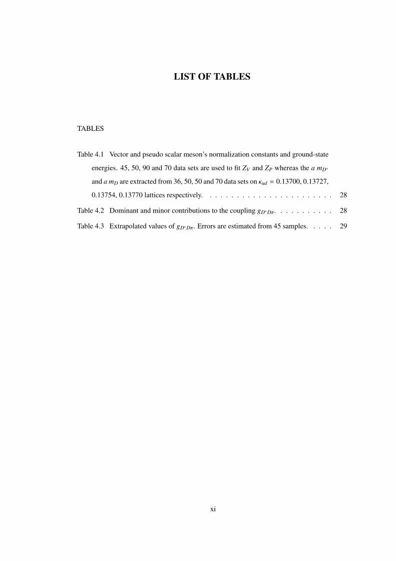
Table 4.1 Vector and pseudo scalar meson’s normalization constants and ground-state

energies. 45, 50, 90 and 70 data sets are used to fit ZV and ZP whereas the a mD∗

and a mD are extracted from 36, 50, 50 and 70 data sets on κud = 0.13700, 0.13727,

0.13754, 0.13770 lattices respectively. . . . . . . . . . . . . . . . . . . . . . . . 28

Table 4.2 Dominant and minor contributions to the coupling gD∗Dπ. . . . . . . . . . . 28

Table 4.3 Extrapolated values of gD∗Dπ. Errors are estimated from 45 samples. . . . . 29

xi

LIST OF FIGURES

FIGURES

Figure 1.1 Running of the strong coupling constant, αs, [3]. . . . . . . . . . . . . . . 2

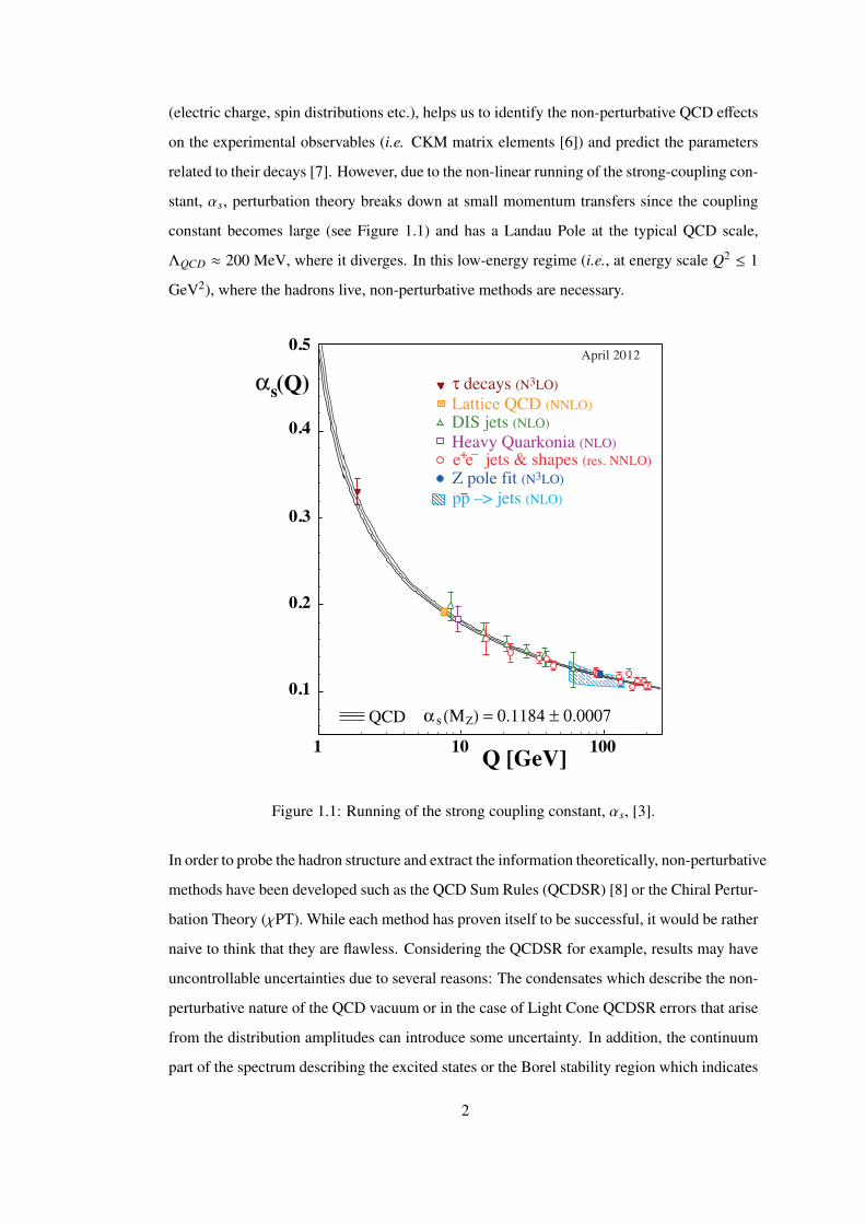
Figure 1.2 Remarkable Lattice QCD results: Hadron spectroscopy (up) and running

coupling constant (down), compare with Figure 1.1. Plots are from Ref. [1] and [4]

respectively. . . . . . . . . . . . . . . . . . . . . . . . . . . . . . . . . . . . . . 4

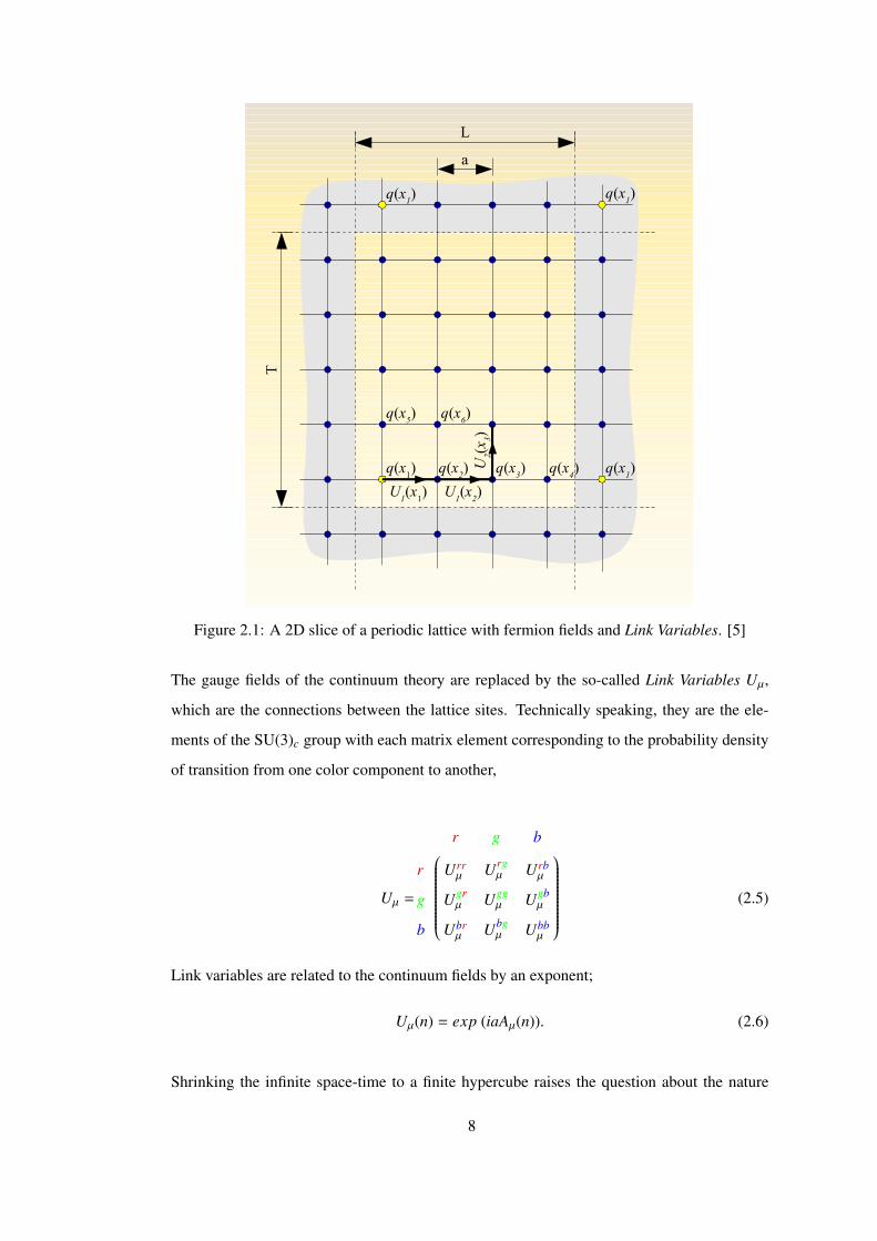
Figure 2.1 A 2D slice of a periodic lattice with fermion fields and Link Variables. [5] 8

Figure 2.2 Forward and backward link variables (left) and 1 × 1 Plaquette Uµν, con-

structed from four link variables (right). . . . . . . . . . . . . . . . . . . . . . . . 12

Figure 2.3 Plaquette and rectangular loop contributions to Iwasaki action . . . . . . . 17

Figure 2.4 Sum of plaquettes in the µ-ν plane. Compare with Eq. (2.21) and Figure 2.2. 18

Figure 3.1 Feynman diagram of R1(t). Curved double lines indicate the heavy quark,

grey dots are the shell smeared sources and vertical double lines are the wall

smeared sinks. . . . . . . . . . . . . . . . . . . . . . . . . . . . . . . . . . . . . 24

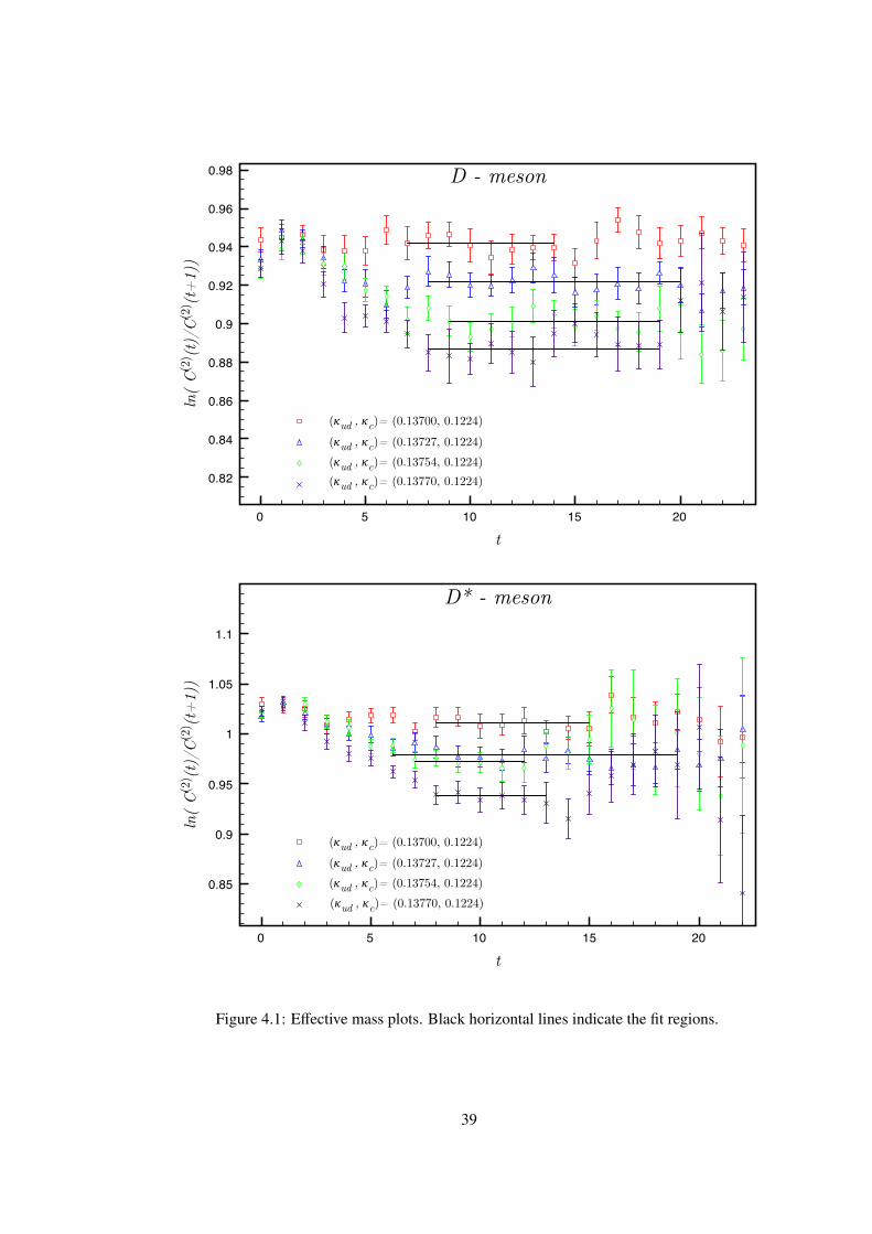
Figure 4.1 Effective mass plots. Black horizontal lines indicate the fit regions. . . . . 39

Figure 4.2 Fit regions for gD∗Dπ with error bands. Plots are given for κud = 0.13700,

0.13727. . . . . . . . . . . . . . . . . . . . . . . . . . . . . . . . . . . . . . . . 40

Figure 4.3 Fit regions for gD∗Dπ with error bands. Plots are given for κud = 0.13754,

0.13770. . . . . . . . . . . . . . . . . . . . . . . . . . . . . . . . . . . . . . . . 41

Figure 4.4 gD∗Dπ as a function of m2π in lattice units. The black data points are simu-

lated on configurations with κud = (0.13700, 0.13727, 0.13754, 0.13770) corre-

sponding to mπ = (700, 570, 410, 300)MeV. The blue point is the experimental

value. . . . . . . . . . . . . . . . . . . . . . . . . . . . . . . . . . . . . . . . . . 42

xii

CHAPTER 1

INTRODUCTION

We can describe the three of the four known forces with the Standard Model (SM) of the

particle physics. This model constructs the theoretical foundations of the electromagnetic,

weak and strong interactions of elementary particles and enables us to study the Nature in

a systematic fashion. The SM is a gauge theory with the gauge group SU(3)×SU(2)×U(1)

where the SU(2)×U(1) group constitutes the electroweak sector of the SM whereas the SU(3)

is the gauge group of Quantum Chromo Dynamics (QCD) and governs the strong interactions.

The elementary particles are classified as the Fermions and the Bosons. Fermion sector holds

three families of quarks and leptons and their anti-particles with half-integer spins (e.g. 1/2,

3/2, . . . ), and the Boson sector has force carrying particles, the Gauge Bosons, with integer

spins (e.g. 0, 1, . . . ). The quarks and gluons, apart from spin and charge quantum numbers

like leptons and bosons, also carry a color quantum number, which leads to the strong in-

teractions among them and the self-interactions of the gluons. One peculiarity of the strong

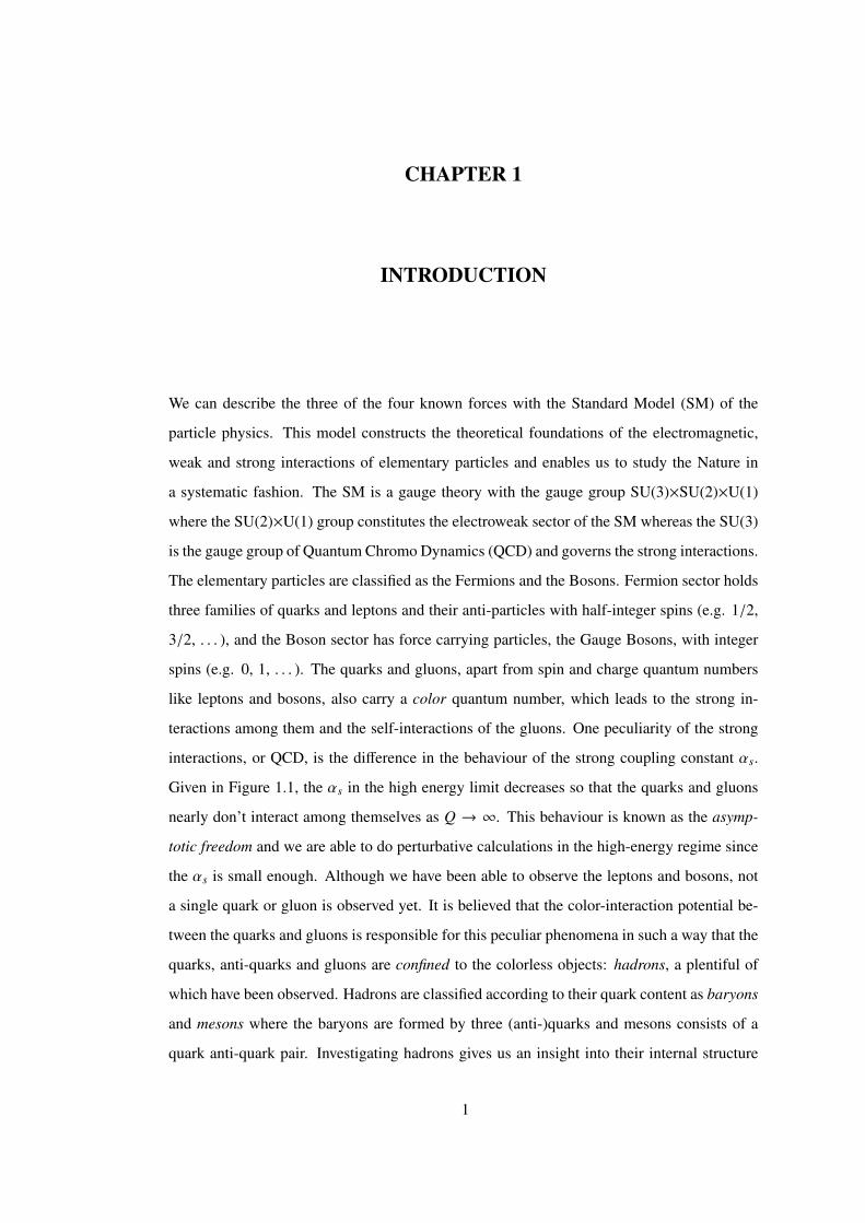
interactions, or QCD, is the difference in the behaviour of the strong coupling constant αs.

Given in Figure 1.1, the αs in the high energy limit decreases so that the quarks and gluons

nearly don’t interact among themselves as Q → ∞. This behaviour is known as the asymp-

totic freedom and we are able to do perturbative calculations in the high-energy regime since

the αs is small enough. Although we have been able to observe the leptons and bosons, not

a single quark or gluon is observed yet. It is believed that the color-interaction potential be-

tween the quarks and gluons is responsible for this peculiar phenomena in such a way that the

quarks, anti-quarks and gluons are confined to the colorless objects: hadrons, a plentiful of

which have been observed. Hadrons are classified according to their quark content as baryons

and mesons where the baryons are formed by three (anti-)quarks and mesons consists of a

quark anti-quark pair. Investigating hadrons gives us an insight into their internal structure

1

(electric charge, spin distributions etc.), helps us to identify the non-perturbative QCD effects

on the experimental observables (i.e. CKM matrix elements [6]) and predict the parameters

related to their decays [7]. However, due to the non-linear running of the strong-coupling con-

stant, αs, perturbation theory breaks down at small momentum transfers since the coupling

constant becomes large (see Figure 1.1) and has a Landau Pole at the typical QCD scale,

ΛQCD ≈ 200 MeV, where it diverges. In this low-energy regime (i.e., at energy scale Q2 ≤ 1

GeV2), where the hadrons live, non-perturbative methods are necessary.

9. Quantum chromodynamics 31

Notwithstanding these open issues, a rather stable and well defined world averagevalue emerges from the compilation of current determinations of !s:

!s(M2Z) = 0.1184 ± 0.0007 .

The results also provide a clear signature and proof of the energy dependence of !s, infull agreement with the QCD prediction of Asymptotic Freedom. This is demonstrated inFig. 9.4, where results of !s(Q

2) obtained at discrete energy scales Q, now also includingthose based just on NLO QCD, are summarized and plotted.

Figure 9.4: Summary of measurements of !s as a function of the respective energyscale Q. The respective degree of QCD perturbation theory used in the extractionof !s is indicated in brackets (NLO: next-to-leading order; NNLO: next-to-next-toleading order; res. NNLO: NNLO matched with resummed next-to-leading logs;N3LO: next-to-NNLO).

June 29, 2012 14:54

Figure 1.1: Running of the strong coupling constant, αs, [3].

In order to probe the hadron structure and extract the information theoretically, non-perturbative

methods have been developed such as the QCD Sum Rules (QCDSR) [8] or the Chiral Pertur-

bation Theory (χPT). While each method has proven itself to be successful, it would be rather

naive to think that they are flawless. Considering the QCDSR for example, results may have

uncontrollable uncertainties due to several reasons: The condensates which describe the non-

perturbative nature of the QCD vacuum or in the case of Light Cone QCDSR errors that arise

from the distribution amplitudes can introduce some uncertainty. In addition, the continuum

part of the spectrum describing the excited states or the Borel stability region which indicates

2

the independence to the unphysical Borel-Mass parameter may be misidentified. Despite

these uncertainties QCDSR provide us very valuable information regarding the hadronic ob-

servables (see [9, 10] and references therein). χPT [11, 12] on the other hand, is an effective

field theory formulated as a perturbative expansion over mπ and contains the coupling con-

stants as input parameters which have to be fitted to the experimental data or calculated from

other theoretical methods.

One other promising non-perturbative method is Lattice QCD (LQCD). It is an ab initio

method starting directly from the QCD Lagrangian which simulates the strong interactions

numerically on a discretized Euclidean space-time. LQCD method has proven itself over

years and has become even more reliable with technological and algorithmic advancements

in the last years. Some of its remarkable achievements are the precise spectroscopy mea-

surements [1] and the prediction for the behavior of the running coupling constant [4] (see

Figure 1.2) consistent with the experiments. Lattice community actively studies the hadronic

observables to gain a better perspective on the hadron structure and interactions, as well as to

provide valuable input to other methods [13].

These non-perturbative methods have been applied to light (u, d, s) and heavy (c, b) quark

sectors extensively but the charm sector still requires more attention from LQCD. Charm

physics plays a significant role in understanding the quark-gluon plasma, a new phase of the

QCD matter where quarks and gluons are believed to live as free particles. The suppression

of the charmonium state J/ψ is considered as a signal for the formation of this new phase.

It is possible that J/ψ can be absorbed by light mesons (i.e. π, ρ) or nucleons (see ref. [14])

abundant in the later stages of the heavy ion collisions like the ones in RHIC or LHC’s Pb-Pb

collisions. Below are some possible absorption reactions that may occur.

π + J/ψ→ D + D∗, D + D∗

ρ + J/ψ→ D + D

N + J/ψ→ Λc + D

We see that specific coupling constants at the hadronic vertices (e.g. gD∗Dπ etc.) are needed

to give an accurate description of charm-hadron production and suppression in collisions per-

formed at RHIC.

3

0 0.01 0.02 0.03

mAWI

0.5

0.6

0.7

0.8

0.9

1.0

!s=0.13640!s=0.13660linearphysical ptExperiment

ud

m"

0 0.01 0.02 0.03

mAWI

0.5

0.6

0.7

0.8

0.9

1.0

!s=0.13640!s=0.13660linearphysical ptExperiment

ud

m#$

0 0.01 0.02 0.03

mAWI

0.6

0.7

0.8

0.9

1.0

1.1

!s=0.13640!s=0.13660linearphysical ptExperiment

ud

m%$

0 0.01 0.02 0.03

mAWI

0.6

0.7

0.8

0.9

1.0

1.1

!s=0.13640!s=0.13660linearphysical ptExperiment

ud

m&

FIG. 23 (color online). Same as Fig. 21 for the decuplet baryons.

0.0

0.5

1.0

1.5

2.0

'K

*(

N

) #%

"#$

%$&

vector meson octet baryon decuplet baryon

mass [GeV]

FIG. 24 (color online). Light hadron spectrum extrapolated tothe physical point using m!, mK and m! as input. Horizontalbars denote the experimental values.

0 1 2 3 4 5 6 7 8 9t

1.00

1.50

2.00

1.10

1.20

1.30

0.88

0.92

0.96

1.00Veff(r=4)

Veff(r=8)

Veff(r=12)

FIG. 25. Effective potential Veff!r; t" with r # 4, 8, 12 at"ud # 0:13770 as a representative case.

S. AOKI et al. PHYSICAL REVIEW D 79, 034503 (2009)

034503-24

2

gluon Green functions (dressing functions). The proce-dure to compute the coupling defined by (1), and fromit to extract an estimate of Λms, is described in verydetail in refs. [10, 11] and we recently applied this inref. [3] to compute Λms from Nf=2+1+1 gauge config-urations for several bare couplings, light twisted massesand volumes. The prescriptions applied for the appropri-ate elimination of discretization artefacts, as the so-calledH(4)-extrapolation procedure to cure the artefacts whichare due to the breaking of the rotational invariance on thelattice [12], needed to be provided with reliable and ex-ploitable results were also carefully shown and explainedin ref. [3]. After this, we are left with the lattice estimatesof the Taylor coupling computed over a large range ofmomenta that, as can be seen in fig. 1, can be describedabove around 4 GeV by the following OPE formula:

αT (µ2) = αpertT (µ2)

1 +

9

µ2Rαpert

T (µ2),αpertT (q2

0)

×αpert

T (µ2)

αpertT (q2

0)

1−γA2

0 /β0g2

T (q20)A2R,q2

0

4(N2C − 1)

, (2)

derived from the OPE description of ghost and gluondressing functions [11], where γA2

0 can be taken from

[13, 14] to give for Nf = 4, 1 − γA2

0 /β0 = 27/100,and, applying the same method outlined in the ap-pendix of ref. [11], one can take advantage of the O(α4)-computations for the Wilson coefficients in ref. [14], andobtains R(α,α0) for q0 = 10 GeV (see Eq.(6) of [3]). Thepurely perturbative running in Eq. (2) is given up to four-loops by integration of the β-function [4], where its coef-ficients are taken to be defined in Taylor-scheme [10, 15].The inclusion of the non-perturbative OPE correction isunavoidable to properly describe the running of the cou-pling over the accesible momentum range, at least abovearound 4 GeV. This however allows to fit both g2A2and ΛT , the ΛQCD parameter in Taylor scheme, throughthe comparison of the prediction given by Eq. (2) andthe lattice estimate of Taylor coupling. The best-fit ofEq. (2) to the lattice data published in ref. [3] can be seenin the plot of Fig. 1 (dotted line), while the best-fittedparameters should be read in Tab. I. In this letter, wealso update the analysis by including an “ad-hoc” correc-tion to account for higher power corrections (suggestedby the detailed analysis of ref. [3]) that allows to extendthe fitting window down to p 1.7 GeV. Furthermore,in addition to the lattice ensembles of gauge configura-tions described in ref. [3], we study 60 more at β = 2.1(aµl = 0.002) and three new ensembles of 50 configura-tions at β = 1.9 and aµl = 0.003, 0.004, 0.005 to peform achiral extrapolation for the ratios of lattice spacings andget: a(2.1, 0.002)/a(1.9, 0) = 0.685(21). Thus, we havefinally converted our estimates to physical units with the

previous ratio and the lattice size in the chiral limit atβ = 1.9 [8]: 0.08612(42) fm. .

2 3 4 5 6 7

p (GeV)

0.5!T(p

)

"=1.95, aµl=0.0055

"=2.1, aµl=0.0020

"=1.95, aµl=0.0035

OPE + d/p6

OPE

FIG. 1: The strong running coupling in Taylor scheme definedby (1) obtained over a large momentum range from latticeQCD, as described in ref. [3]. The dotted line stands herefor the best-fit with Eq. (2), while the solid one includes ahigher-order power correction effectively behaving as ∼ 1/p6.

THE WILSON OPE COEFFICIENT AND THEHIGHER-POWER CORRECTIONS

The OPE prediction for αT given by Eq. (2) is dom-inated by the first correction introduced by the non-vanishing dimension-two landau-gauge gluon conden-sate [16–21], where the Wilson coefficient is applied atthe O(α4)-order. In the previous technical paper [3], weprovided with a strong indication that the OPE anal-ysis is indeed in order: it was clearly shown that thelattice data could be only explained by including non-perturbative contributions and that the Wilson coeffi-cient for the Landau-gauge gluon condensate was neededto describe the behaviour of data above p 4 GeV.

In Fig. 2, the impact of higher-power corrections isanalized. The plot shows the departure of the latticedata for the Taylor coupling from the prediction givenby Eq. (2), plotted in terms of the momentum, with log-arithmic scales for both axes. The data seem to indi-cate that the next-to-leading non-perturbative correctionis highly dominated by an 1/p6 term. This might sug-gest that the 1/p4 OPE contributions are negligible whencompared with the 1/p6 ones or that the product of theleading 1/p4 terms and the involved Wilson coefficientsleave with an effective 1/p6 behaviour. Anyhow, this im-plies that we can effectively describe the lattice data forthe Taylor coupling with

αdT (p2) = αT (p2) +

d

p6, (3)

where d is a free parameter to be fitted, which we donot attribute to any particular physical meaning, for all

Figure 1.2: Remarkable Lattice QCD results: Hadron spectroscopy (up) and running couplingconstant (down), compare with Figure 1.1. Plots are from Ref. [1] and [4] respectively.

In this work we concentrate on one particular hadronic observable: The D∗Dπ coupling con-

stant, gD∗Dπ. The reason we choose this coupling is primarily because there is enough phase

space for D∗ → Dπ decay and it is possible to compare our result to experimental data ob-

tained from CLEO II experiment [15].

There are several results available in the literature estimated by both QCDSR and LQCD.

QCDSR calculations, however, underestimate the D∗Dπ coupling constant(e.g. g(QCDS R)D∗Dπ =

9 ± 2 or g(LCQCDS R))D∗Dπ = 11 ± 2. See Ref. [16]) compared to its experimental value, g(exp)

D∗Dπ =

17.9 ± 0.3 ± 1.9. An earlier LQCD result [17] on the other hand is in good agreement with

experiment, g(lqcd)D∗Dπ = 18.8 ± 2.3+1.1

−2.0. This lattice result was obtained on 243 × 64 quenched

4

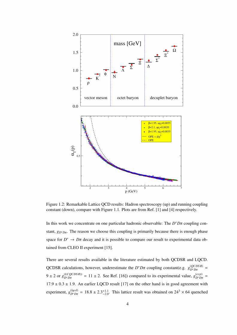
(sea-quark effects ignored) lattices. We estimate our results from simulations on 323 × 64 un-

quenched (with sea-quark effects), 2 + 1-flavor (u, d, s) lattices and with a different simulation

method than used in Ref. [17].

This thesis is organized as follows. In Chapter 2 we discuss the Lattice-QCD method by

demonstrating how to discretize the space-time and continuum action and sketch the typical

workflow. The method we use and the simulation details are given in Chapter 3. We present

our results and discuss the possible source of errors in Chapter 4. Conclusions are summarized

in Chapter 5.

5

CHAPTER 2

LATTICE QCD

Like any other renormalizable quantum field theory, QCD needs an ultraviolet regularization

if we want to extract physical information. Discretizing the space-time to a lattice introduces

an intrinsic momentum cut-off proportional to the inverse of the lattice spacing “a” and pro-

vides a regularization per se. In addition to regularization, we should also consider how to

quantize our theory. Euclidean path-integral formalism governs the quantization of the lattice

theory and is the main instrument to calculate the physical observables. Correlation func-

tions give access to the observables, namely the hadronic properties such as the energy of the

hadron or the matrix elements:

limT→∞

⟨O2(t)O1(0)

⟩T =

∑h

⟨0|O2|h

⟩⟨h|O1|0

⟩e−Eht (2.1)

and in the path-integral formalism we can write,

⟨O2(t)O1(0)

⟩=

1ZT

∫D[Ψ]e−S E[Ψ]O2[Ψ(~x, t)]O1[Ψ(~x, 0)] (2.2)

where O2(t), O1(0) are the Euclidean operators, Eh is the energy of the intermediate hadronic

state, ZT is the partition function, ZT =∫D[Ψ]e−S E[Ψ], and S E is the Euclidean action. The

hadron operators O1 and O2 create(annihilate) the hadronic states with the quantum numbers

that they carry, which in turn creates(annihilates) not only the ground state but also the excited

states of the hadron in question. The limit description in Eq. (2.1) ensures that, as the time

evolves only the ground state survives.

The choice of Euclidean space-time holds the key to solve the theory numerically. It is real-

6

ized by a Wick rotation to imaginary time and Eq. (2.2) shows two notable benefits of such

t → −it transformation: i) This rotation clearly reveals the resemblance between the sta-

tistical and quantum field theories, enabling the use of statistical methods such as Monte

Carlo integration, where the e−S E term is interpreted as the weight factor. ii) In contrast to

the Minkowski version the wildly oscillating exponent is now an exponential decay, e−S E ,

changing the integral to a well-behaved function.

The path integral formalism is suitable to solve with Monte Carlo integration on a finite lattice,

however the underlying theory should also be discretized like the lattice itself. The following

sections cover the naive discretization of fermions, Wilson Gauge action and the improved

discretized actions used in this work.

2.1 Discrete Space-time and QCD

Throughout this section, we follow the Gattringer & Lang’s [18] notation.

2.1.1 Discrete Space-time

The first thing to do is to replace the continuum space-time with the discrete 4D lattice. Let’s

denote it by Λ:

Λ =

n = (n1, n2, n3, n4), | n1,2,3 = 0, 1, . . . ,N − 1,

n4 = 0, 1, . . . ,NT − 1,

(2.3)

where NT is the total number of the time steps and N is the total number of the spatial steps.

We impose the condition that the fermion fields are restricted to the lattice sites and allowed

to move step by step on straight lines only,

ψ(x)→ a−3/2 ψ(an), ψ(x)→ a−3/2 ψ(an), (2.4)

where n is the coordinate vector (~n, n4) and “a” is the lattice spacing, which we drop for

simplicity.

7

LATTICE QCD Lattice QCD = QCD in discrete (Euclidean) space-time

periodic lattice, spacing a,box size L3 ! T .

quarks q(x) live on nodes,gluons Uµ(x) live on links

The lattice QCD action is

gauge invariant under SU(3)C

not unique" O(a)-improved actions

as a " 0: same spectrum &dispersion relation as continuumQCD for low-momentum modes

B. Musch (TUM) Extended Gauge Link Operators 2007-07-05 4 / 55

quarks

on lattice sites

n

gauge fields (gluons)

on links

limits / extrapolations required:

a ! 0 L ! " mq ! mphysq

lattice spacing: lattice volume: quark masses:

!(x) = (u(x), d(x), s(x), . . .)T

QCD in discretized Euclidean space-time using powerful computers

U(x ! y) = P exp

!"

" y

x

dx!µAµ(x!)

#

Figure 2.1: A 2D slice of a periodic lattice with fermion fields and Link Variables. [5]

The gauge fields of the continuum theory are replaced by the so-called Link Variables Uµ,

which are the connections between the lattice sites. Technically speaking, they are the ele-

ments of the SU(3)c group with each matrix element corresponding to the probability density

of transition from one color component to another,

Uµ =

r g b

r Urrµ Urg

µ Urbµ

g Ugrµ Ugg

µ Ugbµ

b Ubrµ Ubg

µ Ubbµ

(2.5)

Link variables are related to the continuum fields by an exponent;

Uµ(n) = exp (iaAµ(n)). (2.6)

Shrinking the infinite space-time to a finite hypercube raises the question about the nature

8

of the boundaries, whether the lattice should have periodic or anti-periodic boundary con-

ditions. For our purposes we choose periodic boundary conditions to conserve the discrete

translational symmetry.

ψ(0, n2, n3, n4) = ψ(N, n2, n3, n4) Uµ(N, n2, n3, n4) = Uµ(0, n2, n3, n4)

...... (2.7)

ψ(n1, n2, n3, 0) = ψ(n1, n2, n3,NT ) Uµ(n1, n2, n3,NT ) = Uµ(n1, n2, n3, 0)

Now we have discretized the main components, all we need to do is to reformulate our theory

accordingly.

2.1.2 Discrete QCD

The familiar continuum QCD action is as follows:

S [ψ, ψ, A] =

N f∑f =1

∫d4x ψ( f )(x)αc[∂/ + igA/(x) + m( f )]ψ( f )(x)αc +

12

∫d4x Tr[FµνFµν] (2.8)

where ψ( f )(x)αc, ψ( f )(x)αc are the fermion, anti-fermion spinors with Dirac, flavor and color

indices α, f and c, respectively. Aµ is the gauge field, g is the strong coupling constant and

Fµν is the field strength tensor,

Fµν = ∂µAν(x) − ∂νAµ(x) + ig[Aµ, Aν]. (2.9)

Taking the color components of the gauge fields into account,

Aµ(x) =

8∑i=1

Aiµ(x)Ti , (2.10)

we can rewrite Eq. (2.9) as,

Fµν(x) =

8∑i=1

∂µAi

ν(x) − ∂νAiµ(x) − g f jkiA

jµAk

ν

Ti (2.11)

9

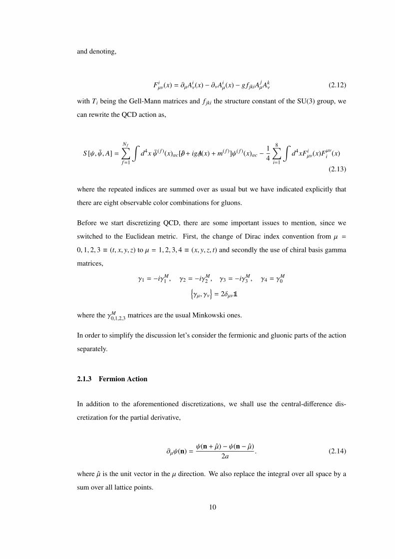
and denoting,

Fiµν(x) = ∂µAi

ν(x) − ∂νAiµ(x) − g f jkiA

jµAk

ν (2.12)

with Ti being the Gell-Mann matrices and f jki the structure constant of the SU(3) group, we

can rewrite the QCD action as,

S [ψ, ψ, A] =

N f∑f =1

∫d4x ψ( f )(x)αc[∂/ + igA/(x) + m( f )]ψ( f )(x)αc −

14

8∑i=1

∫d4xFi

µν(x)Fµνi (x)

(2.13)

where the repeated indices are summed over as usual but we have indicated explicitly that

there are eight observable color combinations for gluons.

Before we start discretizing QCD, there are some important issues to mention, since we

switched to the Euclidean metric. First, the change of Dirac index convention from µ =

0, 1, 2, 3 ≡ (t, x, y, z) to µ = 1, 2, 3, 4 ≡ (x, y, z, t) and secondly the use of chiral basis gamma

matrices,

γ1 = −iγM1 , γ2 = −iγM

2 , γ3 = −iγM3 , γ4 = γM

0γµ, γν

= 2δµν1

where the γM0,1,2,3 matrices are the usual Minkowski ones.

In order to simplify the discussion let’s consider the fermionic and gluonic parts of the action

separately.

2.1.3 Fermion Action

In addition to the aforementioned discretizations, we shall use the central-difference dis-

cretization for the partial derivative,

∂µψ(n) =ψ(n + µ) − ψ(n − µ)

2a. (2.14)

where µ is the unit vector in the µ direction. We also replace the integral over all space by a

sum over all lattice points.

10

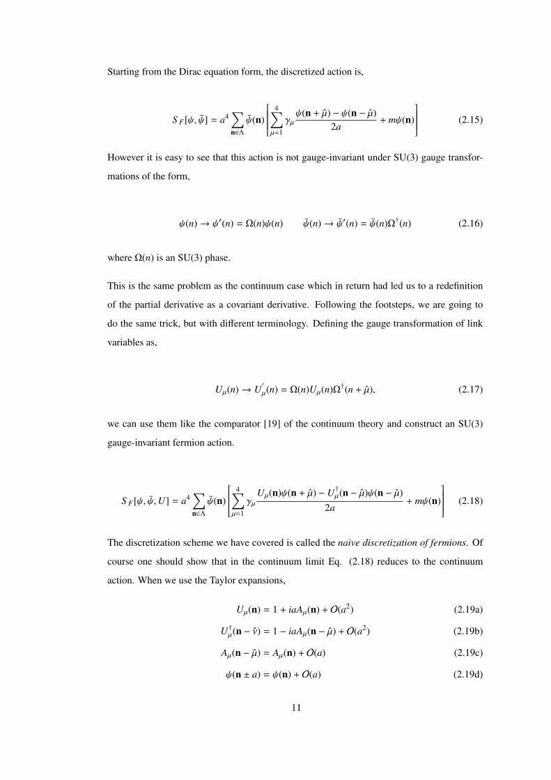
Starting from the Dirac equation form, the discretized action is,

S F[ψ, ψ] = a4∑n∈Λ

ψ(n)

4∑µ=1

γµψ(n + µ) − ψ(n − µ)

2a+ mψ(n)

(2.15)

However it is easy to see that this action is not gauge-invariant under SU(3) gauge transfor-

mations of the form,

ψ(n)→ ψ′(n) = Ω(n)ψ(n) ψ(n)→ ψ′(n) = ψ(n)Ω†(n) (2.16)

where Ω(n) is an SU(3) phase.

This is the same problem as the continuum case which in return had led us to a redefinition

of the partial derivative as a covariant derivative. Following the footsteps, we are going to

do the same trick, but with different terminology. Defining the gauge transformation of link

variables as,

Uµ(n)→ U′

µ(n) = Ω(n)Uµ(n)Ω†(n + µ), (2.17)

we can use them like the comparator [19] of the continuum theory and construct an SU(3)

gauge-invariant fermion action.

S F[ψ, ψ,U] = a4∑n∈Λ

ψ(n)

4∑µ=1

γµUµ(n)ψ(n + µ) − U†µ(n − µ)ψ(n − µ)

2a+ mψ(n)

(2.18)

The discretization scheme we have covered is called the naive discretization of fermions. Of

course one should show that in the continuum limit Eq. (2.18) reduces to the continuum

action. When we use the Taylor expansions,

Uµ(n) = 1 + iaAµ(n) + O(a2) (2.19a)

U†µ(n − ν) = 1 − iaAµ(n − µ) + O(a2) (2.19b)

Aµ(n − µ) = Aµ(n) + O(a) (2.19c)

ψ(n ± a) = ψ(n) + O(a) (2.19d)

11

we recover the continuum action up to O(a),

S F[ψ, ψ,U] = a4∑n∈Λ

4∑µ=1

ψ(n)(γµ∂µ + m

)ψ(n) + ia4

∑n∈Λ

4∑µ=1

ψ(n)γµAµ(n)ψ(n) +O(a). (2.20)

Note that the sum over all lattice points introduces a term proportional to 1/a4, thus the first

two terms are of the order of zero with respect to a.

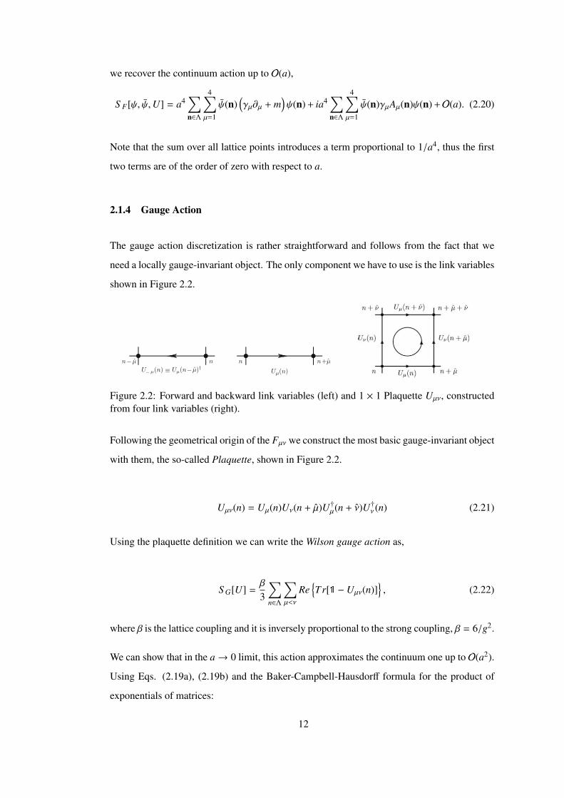
2.1.4 Gauge Action

The gauge action discretization is rather straightforward and follows from the fact that we

need a locally gauge-invariant object. The only component we have to use is the link variables

shown in Figure 2.2.

34 2 QCD on the lattice

U! µ(n) ! Uµ(n" µ)†n n+µ

Uµ(n)

nn" µ

Fig. 2.2. The link variables Uµ(n) and U!µ(n)

points from n to n ! µ and is related to the positively oriented link variableUµ(n ! µ) via the definition

U!µ(n) " Uµ(n ! µ)† . (2.34)

In Fig. 2.2 we illustrate the geometrical setting of the link variables on thelattice. From the definitions (2.34) and (2.33) we obtain the transformationproperties of the link in negative direction

U!µ(n) # U "!µ(n) = !(n)U!µ(n)!(n ! µ)† . (2.35)

Note that we have introduced the gluon fields Uµ(n) as elements of the gaugegroup SU(3), not as elements of the Lie algebra which were used in the con-tinuum. According to the gauge transformations (2.33) and (2.35) also thetransformed link variables are elements of the group SU(3).

Having introduced the link variables and their properties under gaugetransformations, we can now generalize the free fermion action (2.29) to theso-called naive fermion action for fermions in an external gauge field U :

SF [",", U ] = a4!

n#!

"(n)

"4!

µ=1

#µUµ(n)"(n+µ) ! U!µ(n)"(n!µ)

2a+m"(n)

#.

(2.36)

Using (2.30), (2.33), and (2.35) for the gauge transformation properties offermions and link variables, one readily sees the gauge invariance of thefermion action (2.36), SF [",", U ] = SF ["","", U "].

2.2.3 Relating the link variables to the continuum gauge fields

Let us now discuss the link variables in more detail and see how they can berelated to the algebra-valued gauge fields of the continuum formulation. Wehave introduced Uµ(n) as the link variable connecting the points n and n+ µ.The gauge transformation properties (2.33) are consequently governed by thetwo transformation matrices !(n) and !(n + µ)†. Also in the continuum anobject with such transformation properties is known: It is the path-orderedexponential integral of the gauge field Aµ along some curve Cxy connectingtwo points x and y, the so-called gauge transporter:

Figure 2.2: Forward and backward link variables (left) and 1 × 1 Plaquette Uµν, constructedfrom four link variables (right).

Following the geometrical origin of the Fµν we construct the most basic gauge-invariant object

with them, the so-called Plaquette, shown in Figure 2.2.

Uµν(n) = Uµ(n)Uν(n + µ)U†µ(n + ν)U†ν (n) (2.21)

Using the plaquette definition we can write the Wilson gauge action as,

S G[U] =β

3

∑n∈Λ

∑µ<ν

ReTr[1 − Uµν(n)]

, (2.22)

where β is the lattice coupling and it is inversely proportional to the strong coupling, β = 6/g2.

We can show that in the a→ 0 limit, this action approximates the continuum one up to O(a2).

Using Eqs. (2.19a), (2.19b) and the Baker-Campbell-Hausdorff formula for the product of

exponentials of matrices:

12

exp(A)exp(B) = exp(A + B +

12

[A, B] + . . .

), (2.23)

we expand the plaquette,

Uµν = exp(iaAµ(n) + iaAν(n + µ) −a2

2[Aµ(n), Aν(n + µ)]) (2.24)

− iaAµ(n + ν) − iaAν(n) −a2

2[Aµ(n + ν), Aν(n)]) (2.25)

+a2

2[Aν(n + µ), Aµ(n + µ)]) +

a2

2[Aµ(n), Aν(n)]) (2.26)

+a2

2[Aµ(n), Aµ(n + ν)] +

a2

2[Aν(n + µ), Aν(n)]) + O(a3)) (2.27)

and Taylor expanding the resulting fields Aµ(n+ µ) = Aµ(n)+a∂µAµ+O(a2), further simplifies

the plaquette expression,

Uµν = exp(ia2(∂µAν(n) − ∂νAµ + i[Aµ(n), Aν(n)]) + O(a3)) (2.28)

= exp(ia2Fµν(n) + O(a3)), (2.29)

and we see that action reduces to,

S G[U] =β

3

∑n∈Λ

∑µ<ν

ReTr[1 − Uµν(n)]

=

a4

2g2

∑n∈Λ

∑µ<ν

Tr[Fµν(n)2

]+ O(a2). (2.30)

This discrete formulation of QCD was first done by Kenneth G. Wilson in his 1974 paper

[20]. His formulation indeed showed that the physical information can be extracted from

first-principles calculations. However, in the contrary it led to other discretization-related

problems. We have mentioned the discretization errors in sections 2.1.3 and 2.1.4, when

we said that discrete actions approximate the continuum ones up to order O(a) and O(a2)

respectively. Even though one thinks that when we take the continuum limit a → 0, these

errors would go to zero; practically, simulating an a = 0 lattice is impossible for numerical

calculations and these errors will always be counted as systematical errors. Thus, corrections

13

are necessary to improve the discretization errors and to better approximate the continuum

actions. One should keep in mind of course that these correction terms should vanish in

the continuum limit. Iwasaki gauge action [21], Luscher-Weisz gauge action [22], the non-

perturbatively O(a)-improved Wilson fermion action, or also known as the clover action [23]

are some improved actions.

Apart from discretization errors there is also another important problem with the naive dis-

cretization which is the Fermion Doubling. We will deal with this problem in the following

section in the context of our choice of improved fermion action and we will see that we adapt

our solution in the price of explicitly breaking the chiral symmetry. There are other solutions

that take chiral symmetry into account such as the overlap fermions [24] and related domain-

wall fermions [25], staggered fermions [26] and twisted-mass fermions [27] which are out of

the scope of this thesis.

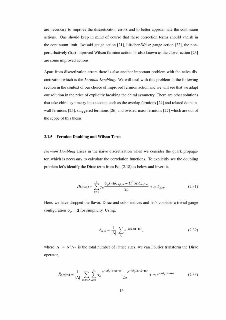
2.1.5 Fermion Doubling and Wilson Term

Fermion Doubling arises in the naive discretization when we consider the quark propaga-

tor, which is necessary to calculate the correlation functions. To explicitly see the doubling

problem let’s identify the Dirac term from Eq. (2.18) as below and invert it.

D(n|m) =

4∑µ=1

γµUµ(n)δn+µ,m − U†µ(n)δn−µ,m

2a+ m δn,m. (2.31)

Here, we have dropped the flavor, Dirac and color indices and let’s consider a trivial gauge

configuration Uµ = 1 for simplicity. Using,

δn,m =1|Λ|

∑kµ

e−iakµ(n−m), (2.32)

where |Λ| = N3NT is the total number of lattice sites, we can Fourier transform the Dirac

operator,

D(n|m) =1|Λ|

∑n,m∈Λ

4∑µ=1

γµe−iakµ(n+µ−m) − e−iakµ(n−µ−m)

2a+ m e−iakµ(n−m) (2.33)

14

by factoring out e−iakµ(n−m) and using Eq. (2.32), we get,

D(n|m) = δn,m

ia

4∑µ=1

sin(kµa)γµ + m1

, (2.34)

where we have also used the Euler’s formula for the sine function and dropped the unit vector

|µ| = 1. Defining the term in parenthesis as D(k) and multiplying the Eq. (2.34) with D(k)−1

from right we find the relation,

D(n|m)D(k)−1 = δn,m (2.35)

which tells us to compute the inverse of the D(k),

D(k)−1 =m1 − ia−1 ∑

µ sin(kµa)γµm2 + a−2 ∑

µ sin2(kµa)(2.36)

and inverse Fourier transform to get the quark propagator D(n|m)−1,

D(n|m)−1 =1|Λ|

∑k∈Λ

D−1(k)e−iak(n−m) (2.37)

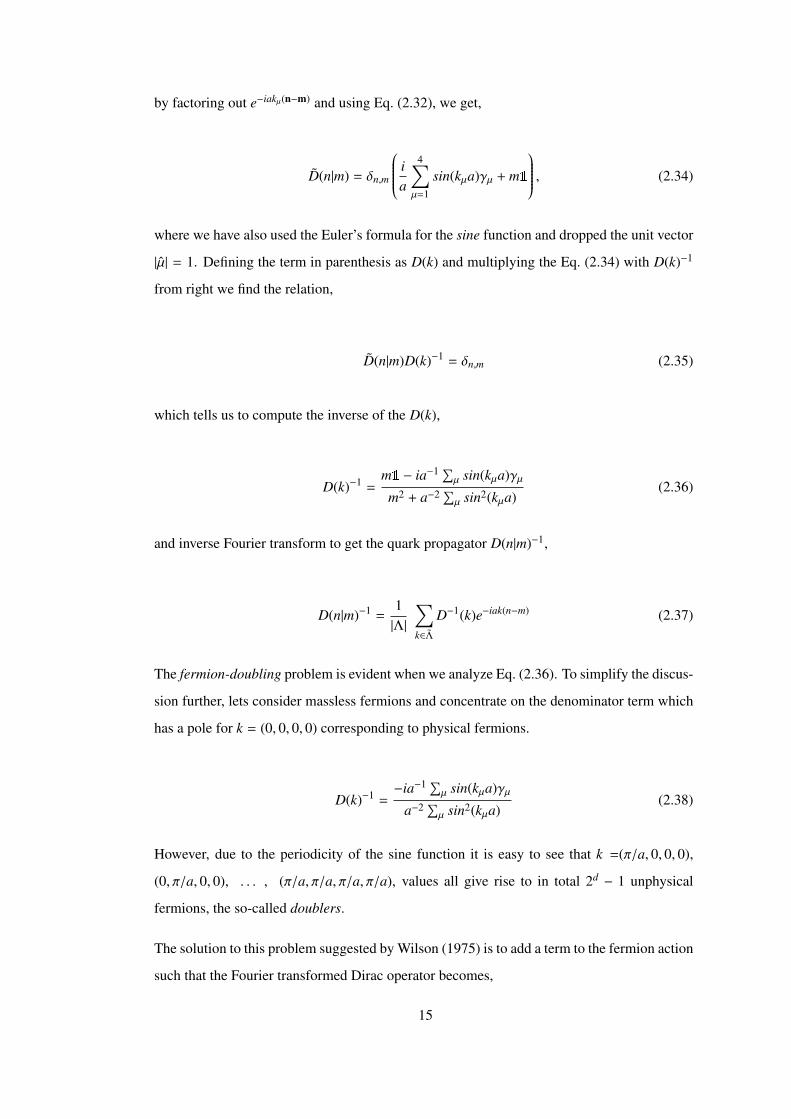
The fermion-doubling problem is evident when we analyze Eq. (2.36). To simplify the discus-

sion further, lets consider massless fermions and concentrate on the denominator term which

has a pole for k = (0, 0, 0, 0) corresponding to physical fermions.

D(k)−1 =−ia−1 ∑

µ sin(kµa)γµa−2 ∑

µ sin2(kµa)(2.38)

However, due to the periodicity of the sine function it is easy to see that k =(π/a, 0, 0, 0),

(0, π/a, 0, 0), . . . , (π/a, π/a, π/a, π/a), values all give rise to in total 2d − 1 unphysical

fermions, the so-called doublers.

The solution to this problem suggested by Wilson (1975) is to add a term to the fermion action

such that the Fourier transformed Dirac operator becomes,

15

D(k) = m1 +ia

4∑µ=1

sin(kµa)γµ + 11a

4∑µ=1

(1 − cos(kµa)

). (2.39)

The relevant term turns out to be the 4D lattice Laplace operator,

−a2 = −a

4∑µ=1

Uµ(n)δn+µ,m − 2δn,m + U†µ(n)δn−µ,m

2a2 (2.40)

where the constant a ensures that the Wilson term vanishes as a → 0. We can write the

corrected Dirac operator as,

D(n|m) =

(m +

4a

)δn,m −

12a

4∑µ=1

[(1 + γµ

)Uµ(n)δn+µ,m +

(1 − γµ

)U†µ(n)δn−µ,m

](2.41)

and the doubler-free Wilson fermion action becomes,

S WF [ψ, ψ,U] = a4

∑n,m∈Λ

ψ(n)D(n|m)ψ(m). (2.42)

As mentioned before, the 4/a factor introduced by the Wilson term explicitly breaks the chiral

symmetry which in turn forces us to perform chiral extrapolations.

For future discussions we will do a factorization of the Dirac term and introduce the hopping

parameter κ, which is an important lattice parameter:

D(n|m) = C(1 − κH(n|m)), κ =1

2(ma + 4), C = m +

4a

H(n|m) =

4∑µ=1

[(1 + γµ

)Uµ(n)δn+µ,m +

(1 − γµ

)U†µ(n)δn−µ,m

].

(2.43)

2.1.6 Improved Actions

One should control the systematical errors due to discretization in order to obtain more reli-

able results. This is best done by improving the actions to have smaller discretization errors.

We showed in subsequent sections that naive fermion and gauge actions have O(a) and O(a2)

discretization errors respectively. It is common sense to use actions that have same discretiza-

tion errors. We now briefly discuss the improved actions used in this work.

16

2.1.6.1 Iwasaki Gauge Action

Since we do not generate lattices but instead use the ones generated by PACS-CS collabora-

tion, we are not directly involved in the choice of gauge action; so we refer to the related paper

for details [1] and references therein. Here we briefly discuss the Iwasaki action. PACS-CS

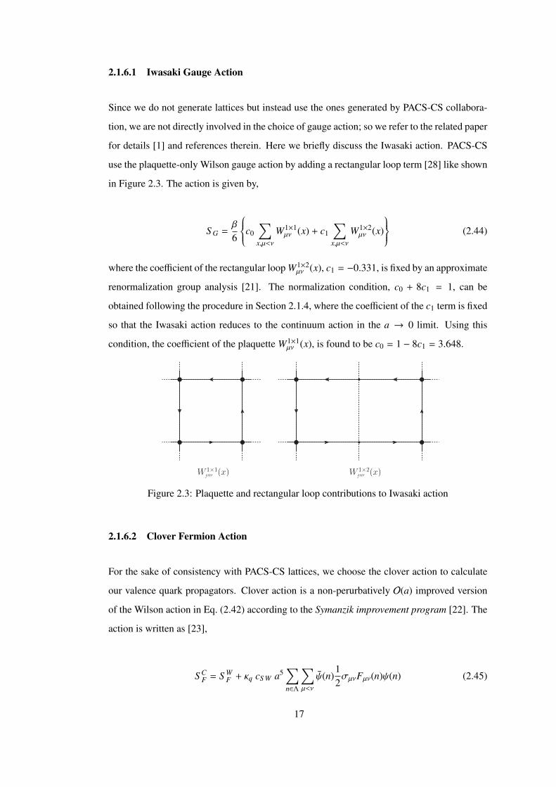
use the plaquette-only Wilson gauge action by adding a rectangular loop term [28] like shown

in Figure 2.3. The action is given by,

S G =β

6

c0

∑x,µ<ν

W1×1µν (x) + c1

∑x,µ<ν

W1×2µν (x)

(2.44)

where the coefficient of the rectangular loop W1×2µν (x), c1 = −0.331, is fixed by an approximate

renormalization group analysis [21]. The normalization condition, c0 + 8c1 = 1, can be

obtained following the procedure in Section 2.1.4, where the coefficient of the c1 term is fixed

so that the Iwasaki action reduces to the continuum action in the a → 0 limit. Using this

condition, the coefficient of the plaquette W1×1µν (x), is found to be c0 = 1 − 8c1 = 3.648.

W 1×1µν (x) W 1×2

µν (x)

Figure 2.3: Plaquette and rectangular loop contributions to Iwasaki action

2.1.6.2 Clover Fermion Action

For the sake of consistency with PACS-CS lattices, we choose the clover action to calculate

our valence quark propagators. Clover action is a non-perurbatively O(a) improved version

of the Wilson action in Eq. (2.42) according to the Symanzik improvement program [22]. The

action is written as [23],

S CF = S W

F + κq cS W a5∑n∈Λ

∑µ<ν

ψ(n)12σµνFµν(n)ψ(n) (2.45)

17

where Sheikholeslami-Wohlert term is found to be cS W = 1.715 [29], σµν = 12 [γµ, γν], κq is

the hopping parameter of the quark and Fµν(n) is discretized as the difference of the sum of

the plaquettes like shown in Figure 2.4,

Fµν(n) =18i

(Qµν(n) − Q†µν(n)

)(2.46)

Qµν(n) = Uµ,ν(n) + Uν,−µ(n) + U−µ,−ν(n) + U−ν,µ(n) (2.47)

9.1 The Symanzik improvement program 217

!

µ

n

Fig. 9.1. Graphical representation of the sum Qµ!(n) of plaquettes in the µ–! planeused for the discretization of the field strength in (9.11)

!Fµ!(n) =!i

8a2(Qµ!(n) ! Q!µ(n)) , (9.11)

where Qµ!(n) is the sum of plaquettes Uµ,!(n) (compare (2.48)) in the µ–!plane as shown in Fig. 9.1,

Qµ!(n) " Uµ,!(n) + U!,!µ(n) + U!µ,!!(n) + U!!,µ(n) , (9.12)

which is a discretization of the continuum field strength tensor. Due to theshape of the terms which is reminiscent of a clover leaf, the last term in (9.10)is often referred to as clover term or clover improvement.

At this point we need to add a couple of comments: We saw that for O(a)improvement it is su!cient to add a single term to the fermion action. The

only pure glue term L(1)3 was found to be proportional to the original gauge

action and thus was absorbed in a redefinition of the bare gauge coupling.Relevant purely gluonic operators appear only at dimension 6, i.e., they con-tribute at O(a2). This is in agreement with previous remarks that for bosonicfields the discretization errors are only of O(a2). For the improvement of thegauge action we refer the reader to the original literature, e.g., [3, 8], wherethe so-called Luscher–Weisz gauge action is presented.

The second comment concerns the discretization errors of chirally sym-metric Dirac operators that obey the Ginsparg–Wilson equation (7.29). If onewould add the order O(a)-improving term, i.e., the clover term, the resultingDirac operator would no longer obey the Ginsparg–Wilson equation. Thuswe must conclude that a Ginsparg–Wilson Dirac operator is already O(a)improved. As a matter of fact the nonlinear right-hand side of the Ginsparg–

Wilson equation (7.29) generates a lattice discretization of the Pauli term L(1)1

when the naive lattice Dirac operator (which necessarily is a building block ofany lattice Dirac operator) is squared. This link between O(a) improvementand chiral symmetry hints already at a nonperturbative strategy [6] for deter-mining the Sheikholeslami–Wohlert coe!cient, which we will present below,following the discussion of the improvement of currents.

Figure 2.4: Sum of plaquettes in the µ-ν plane. Compare with Eq. (2.21) and Figure 2.2.

2.2 Workflow

The idea is to compute the correlation functions and when doing so we need quark propagators

calculated on each individual gauge configuration or lattice. To make things more clear lets

consider such a two-point correlation function,⟨OM(n)OM(m)

⟩= −

1Z

∫D[U]e−S G[U] det[Du] det[Dd] det[Ds]

× Tr[Γ D−1

q1(n|m) Γ D−1

q2(m|n)

]Z =

∫D[U]e−S G[U]det[Du] det[Dd] det[Ds],

(2.48)

where OM(n) and OM(m) are a generic meson’s annihilation, creation operators defined as

OM(n) = q1(n)Γq2(n) and OM(m) = q2(m)Γq1(m), respectively. Determinants det[Du], det[Dd]

and det[Ds] are obtained after integrating out the fermion action and the trace term comes

18

form the quark field contractions according to the Wick’s Theorem. The Γ is a combination

of γ-matrices specific to the meson M.

There are two independent steps in calculating such correlation functions. First one is the

Monte Carlo generation of the lattice according to the “e−S G[U] det[Du] det[Dd] det[Ds]” term

which acts like the Boltzman factor and includes the sea-quark effects via the fermion deter-

minants. Lattice generation is out of the scope of this work and we refer the interested reader

to the Gattringer and Lang’s book [18], which has a nice introductory chapter on generating

gauge configurations. Further techniques related to the configurations used in this work can

be found at the PACS-CS paper [1].

The second step is the computation of the quark propagators D−1f (n|m), on each gauge config-

uration for each flavor f and contract them to find the value of the correlation function. When

this procedure is repeated sufficiently many times one can approximate the integral according

to the importance sampling,

〈O〉 = limN→∞

1N

N∑n=1

O[Un] (2.49)

where O[Un] stands for the value of the function on each gauge configuration.

Ideally, one should calculate such propagators from each site on the lattice for each quark

flavor that forms the hadron, which is extremely time and resource consuming considering

the inversion of the Dirac operator matrix and the high statistical needs. As a workaround one

chooses a source point and computes the propagator from that point to all other lattice sites:

D−1(n|m0) =∑α,a

D−1(n|m)βαba

S (m)αa

(2.50)

A typical choice for the source is a Dirac delta function which, in turn called as a point source.

S (m)αa

= δ(m − m0)δαα0δaa0 (2.51)

where the α and a are the Dirac and color indices. However, if one wants to improve the

ground-state dominance (i.e. ground-state saturation after fewer time steps), then the smeared

sources are favored:

19

S (m) =

N∑i

δ(m − m0)eσ52

(2.52)

52 =

3∑j=1

(U j(n, nt)δ(n + j,m) + U†j (n − j, nt)δ(n − j, nt)

)(2.53)

where N is the number of smearing steps applied to the Dirac delta function and σ is a con-

stant, dimensionless smearing parameter. The set of values for N and σ are chosen so that the

resulting hadron’s root mean square radius is around 1 fm. This type of smearing is known

as gauge-invariant-gaussian smearing or shortly, shell smearing. As a special case, choosing

σ = 0 and summing over all lattice sites leads to wall smearing, which improves ground state

dominance but suffers from large statistical errors.

20

CHAPTER 3

METHOD

3.1 Theory

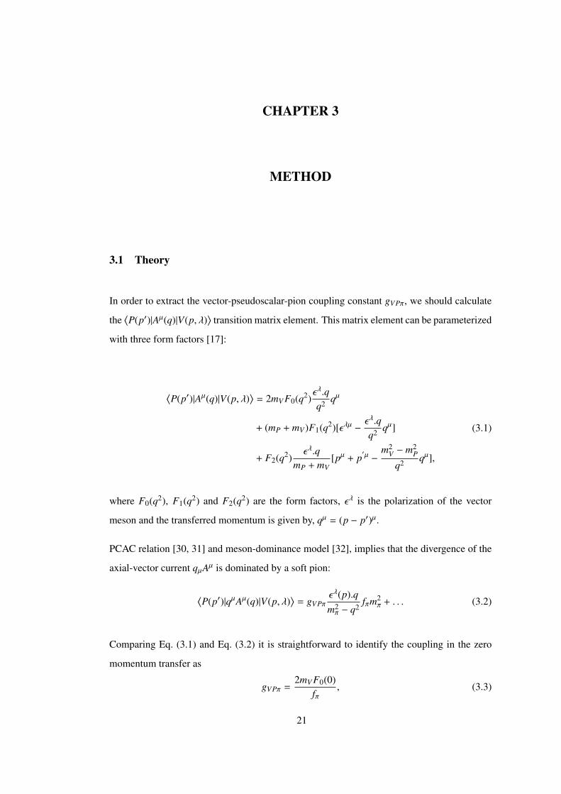
In order to extract the vector-pseudoscalar-pion coupling constant gVPπ, we should calculate

the⟨P(p′)|Aµ(q)|V(p, λ)

⟩transition matrix element. This matrix element can be parameterized

with three form factors [17]:

⟨P(p′)|Aµ(q)|V(p, λ)

⟩= 2mV F0(q2)

ελ.qq2 qµ

+ (mP + mV )F1(q2)[ελµ −ελ.qq2 qµ]

+ F2(q2)ελ.q

mP + mV[pµ + p

′µ −m2

V − m2P

q2 qµ],

(3.1)

where F0(q2), F1(q2) and F2(q2) are the form factors, ελ is the polarization of the vector

meson and the transferred momentum is given by, qµ = (p − p′)µ.

PCAC relation [30, 31] and meson-dominance model [32], implies that the divergence of the

axial-vector current qµAµ is dominated by a soft pion:

⟨P(p′)|qµAµ(q)|V(p, λ)

⟩= gVPπ

ελ(p).qm2π − q2

fπm2π + . . . (3.2)

Comparing Eq. (3.1) and Eq. (3.2) it is straightforward to identify the coupling in the zero

momentum transfer as

gVPπ =2mV F0(0)

fπ, (3.3)

21

where fπ is the pion decay constant.

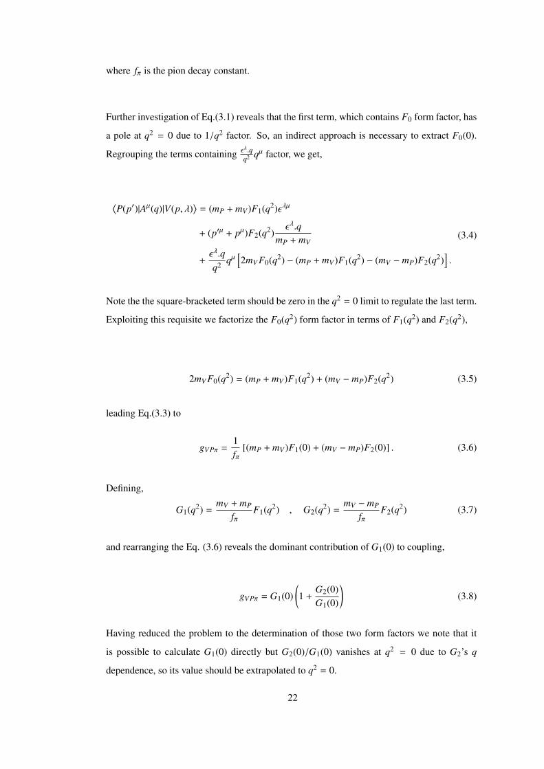
Further investigation of Eq.(3.1) reveals that the first term, which contains F0 form factor, has

a pole at q2 = 0 due to 1/q2 factor. So, an indirect approach is necessary to extract F0(0).

Regrouping the terms containing ελ.qq2 qµ factor, we get,

⟨P(p′)|Aµ(q)|V(p, λ)

⟩= (mP + mV )F1(q2)ελµ

+ (p′µ + pµ)F2(q2)ελ.q

mP + mV

+ελ.qq2 qµ

[2mV F0(q2) − (mP + mV )F1(q2) − (mV − mP)F2(q2)

].

(3.4)

Note the the square-bracketed term should be zero in the q2 = 0 limit to regulate the last term.

Exploiting this requisite we factorize the F0(q2) form factor in terms of F1(q2) and F2(q2),

2mV F0(q2) = (mP + mV )F1(q2) + (mV − mP)F2(q2) (3.5)

leading Eq.(3.3) to

gVPπ =1fπ

[(mP + mV )F1(0) + (mV − mP)F2(0)] . (3.6)

Defining,

G1(q2) =mV + mP

fπF1(q2) , G2(q2) =

mV − mP

fπF2(q2) (3.7)

and rearranging the Eq. (3.6) reveals the dominant contribution of G1(0) to coupling,

gVPπ = G1(0)(1 +

G2(0)G1(0)

)(3.8)

Having reduced the problem to the determination of those two form factors we note that it

is possible to calculate G1(0) directly but G2(0)/G1(0) vanishes at q2 = 0 due to G2’s q

dependence, so its value should be extrapolated to q2 = 0.

22

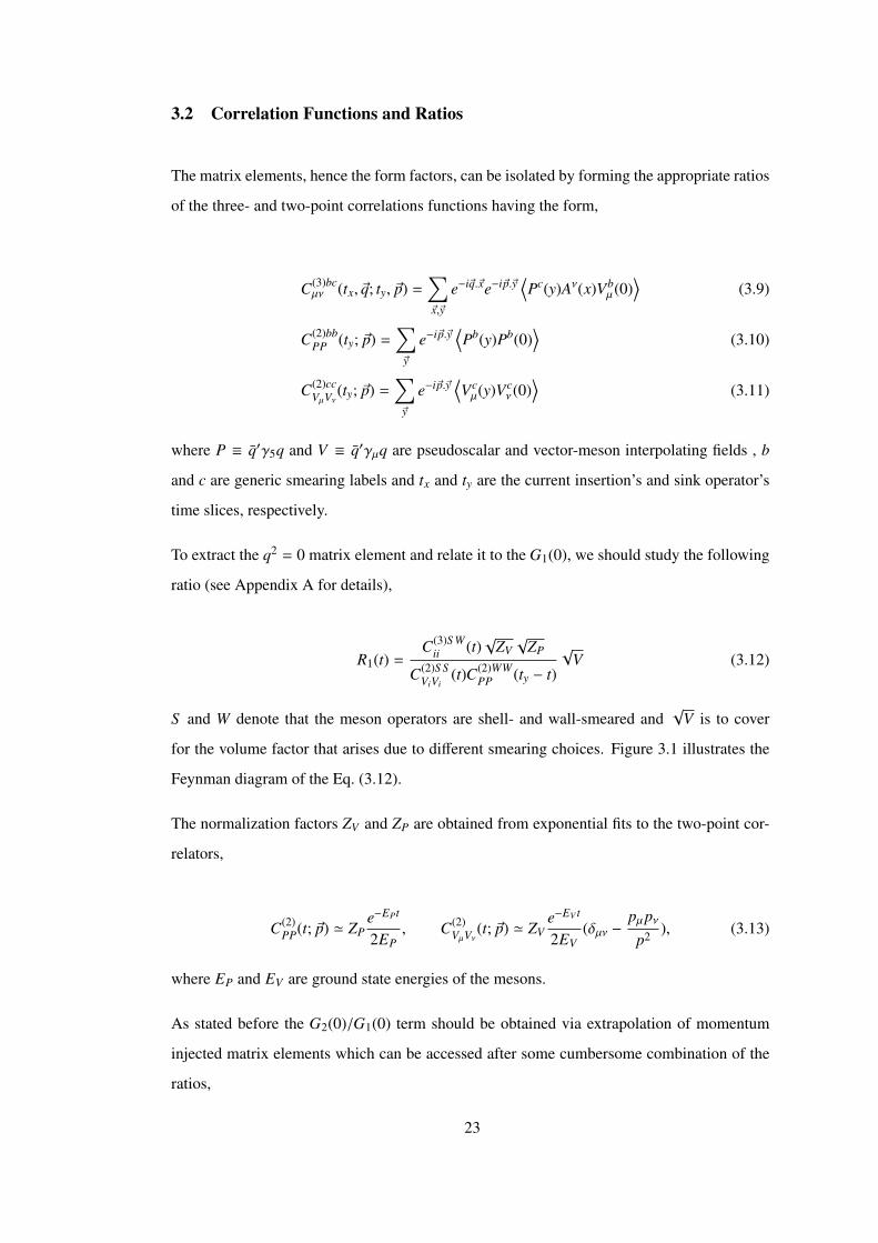
3.2 Correlation Functions and Ratios

The matrix elements, hence the form factors, can be isolated by forming the appropriate ratios

of the three- and two-point correlations functions having the form,

C(3)bcµν (tx, ~q; ty, ~p) =

∑~x,~y

e−i~q.~xe−i~p.~y⟨Pc(y)Aν(x)Vb

µ(0)⟩

(3.9)

C(2)bbPP (ty; ~p) =

∑~y

e−i~p.~y⟨Pb(y)Pb(0)

⟩(3.10)

C(2)ccVµVν

(ty; ~p) =∑~y

e−i~p.~y⟨Vcµ(y)Vc

ν (0)⟩

(3.11)

where P ≡ q′γ5q and V ≡ q′γµq are pseudoscalar and vector-meson interpolating fields , b

and c are generic smearing labels and tx and ty are the current insertion’s and sink operator’s

time slices, respectively.

To extract the q2 = 0 matrix element and relate it to the G1(0), we should study the following

ratio (see Appendix A for details),

R1(t) =C(3)S W

ii (t)√

ZV√

ZP

C(2)S SViVi

(t)C(2)WWPP (ty − t)

√V (3.12)

S and W denote that the meson operators are shell- and wall-smeared and√

V is to cover

for the volume factor that arises due to different smearing choices. Figure 3.1 illustrates the

Feynman diagram of the Eq. (3.12).

The normalization factors ZV and ZP are obtained from exponential fits to the two-point cor-

relators,

C(2)PP(t; ~p) ' ZP

e−EPt

2EP, C(2)

VµVν(t; ~p) ' ZV

e−EV t

2EV(δµν −

pµpνp2 ), (3.13)

where EP and EV are ground state energies of the mesons.

As stated before the G2(0)/G1(0) term should be obtained via extrapolation of momentum

injected matrix elements which can be accessed after some cumbersome combination of the

ratios,

23

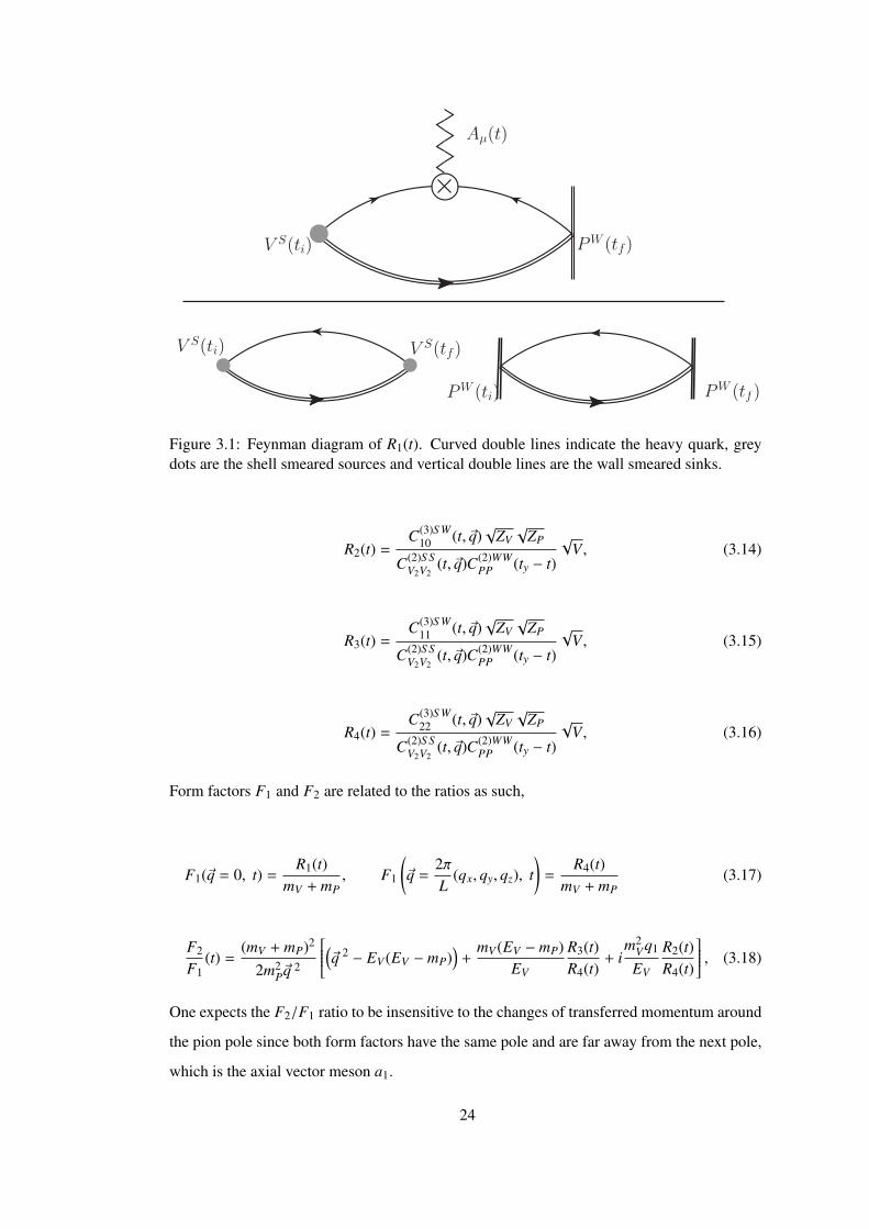
V S(ti) V S(tf)

PW (ti) PW (tf)

V S(ti) PW (tf)

Aµ(t)

Figure 3.1: Feynman diagram of R1(t). Curved double lines indicate the heavy quark, greydots are the shell smeared sources and vertical double lines are the wall smeared sinks.

R2(t) =C(3)S W

10 (t, ~q)√

ZV√

ZP

C(2)S SV2V2

(t, ~q)C(2)WWPP (ty − t)

√V , (3.14)

R3(t) =C(3)S W

11 (t, ~q)√

ZV√

ZP

C(2)S SV2V2

(t, ~q)C(2)WWPP (ty − t)

√V , (3.15)

R4(t) =C(3)S W

22 (t, ~q)√

ZV√

ZP

C(2)S SV2V2

(t, ~q)C(2)WWPP (ty − t)

√V , (3.16)

Form factors F1 and F2 are related to the ratios as such,

F1(~q = 0, t) =R1(t)

mV + mP, F1

(~q =

2πL

(qx, qy, qz), t)

=R4(t)

mV + mP(3.17)

F2

F1(t) =

(mV + mP)2

2m2P~q

2

(~q 2 − EV (EV − mP))

+mV (EV − mP)

EV

R3(t)R4(t)

+ im2

Vq1

EV

R2(t)R4(t)

, (3.18)

One expects the F2/F1 ratio to be insensitive to the changes of transferred momentum around

the pion pole since both form factors have the same pole and are far away from the next pole,

which is the axial vector meson a1.

24

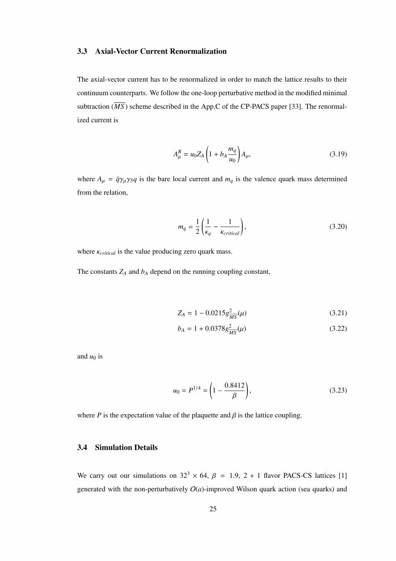
3.3 Axial-Vector Current Renormalization

The axial-vector current has to be renormalized in order to match the lattice results to their

continuum counterparts. We follow the one-loop perturbative method in the modified minimal

subtraction (MS ) scheme described in the App.C of the CP-PACS paper [33]. The renormal-

ized current is

ARµ = u0ZA

(1 + bA

mq

u0

)Aµ, (3.19)

where Aµ = qγµγ5q is the bare local current and mq is the valence quark mass determined

from the relation,

mq =12

(1κq−

1κcritical

), (3.20)

where κcritical is the value producing zero quark mass.

The constants ZA and bA depend on the running coupling constant,

ZA = 1 − 0.0215g2MS

(µ) (3.21)

bA = 1 + 0.0378g2MS

(µ) (3.22)

and u0 is

u0 = P1/4 =

(1 −

0.8412β

), (3.23)

where P is the expectation value of the plaquette and β is the lattice coupling.

3.4 Simulation Details

We carry out our simulations on 323 × 64, β = 1.9, 2 + 1 flavor PACS-CS lattices [1]

generated with the non-perturbatively O(a)-improved Wilson quark action (sea quarks) and

25

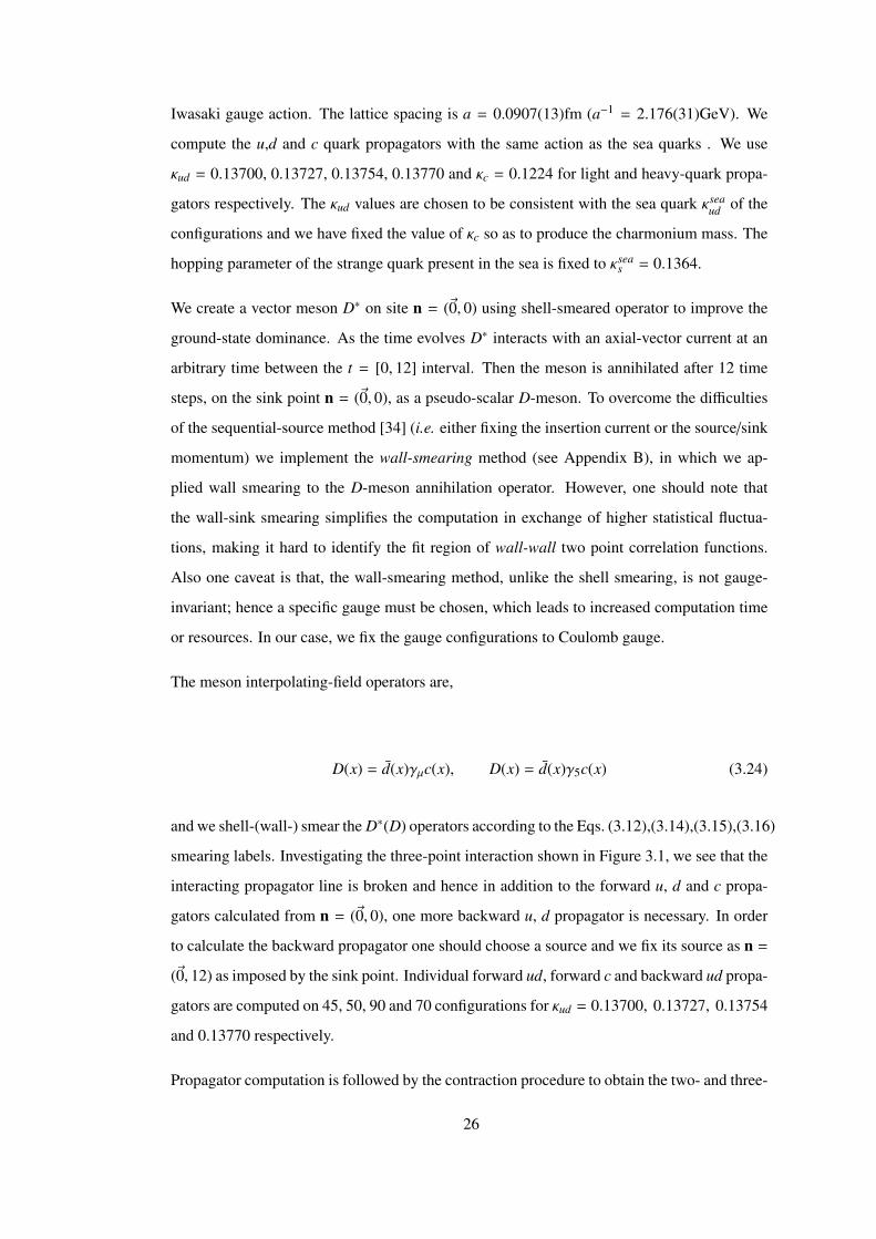
Iwasaki gauge action. The lattice spacing is a = 0.0907(13)fm (a−1 = 2.176(31)GeV). We

compute the u,d and c quark propagators with the same action as the sea quarks . We use

κud = 0.13700, 0.13727, 0.13754, 0.13770 and κc = 0.1224 for light and heavy-quark propa-

gators respectively. The κud values are chosen to be consistent with the sea quark κseaud of the

configurations and we have fixed the value of κc so as to produce the charmonium mass. The

hopping parameter of the strange quark present in the sea is fixed to κseas = 0.1364.

We create a vector meson D∗ on site n = (~0, 0) using shell-smeared operator to improve the

ground-state dominance. As the time evolves D∗ interacts with an axial-vector current at an

arbitrary time between the t = [0, 12] interval. Then the meson is annihilated after 12 time

steps, on the sink point n = (~0, 0), as a pseudo-scalar D-meson. To overcome the difficulties

of the sequential-source method [34] (i.e. either fixing the insertion current or the source/sink

momentum) we implement the wall-smearing method (see Appendix B), in which we ap-

plied wall smearing to the D-meson annihilation operator. However, one should note that

the wall-sink smearing simplifies the computation in exchange of higher statistical fluctua-

tions, making it hard to identify the fit region of wall-wall two point correlation functions.

Also one caveat is that, the wall-smearing method, unlike the shell smearing, is not gauge-

invariant; hence a specific gauge must be chosen, which leads to increased computation time

or resources. In our case, we fix the gauge configurations to Coulomb gauge.

The meson interpolating-field operators are,

D(x) = d(x)γµc(x), D(x) = d(x)γ5c(x) (3.24)

and we shell-(wall-) smear the D∗(D) operators according to the Eqs. (3.12),(3.14),(3.15),(3.16)

smearing labels. Investigating the three-point interaction shown in Figure 3.1, we see that the

interacting propagator line is broken and hence in addition to the forward u, d and c propa-

gators calculated from n = (~0, 0), one more backward u, d propagator is necessary. In order

to calculate the backward propagator one should choose a source and we fix its source as n =

(~0, 12) as imposed by the sink point. Individual forward ud, forward c and backward ud propa-

gators are computed on 45, 50, 90 and 70 configurations for κud = 0.13700, 0.13727, 0.13754

and 0.13770 respectively.

Propagator computation is followed by the contraction procedure to obtain the two- and three-

26

point correlation functions. Two-point correlators are calculated with respect to the three-

point functions’ smearing labels.

27

CHAPTER 4

RESULTS

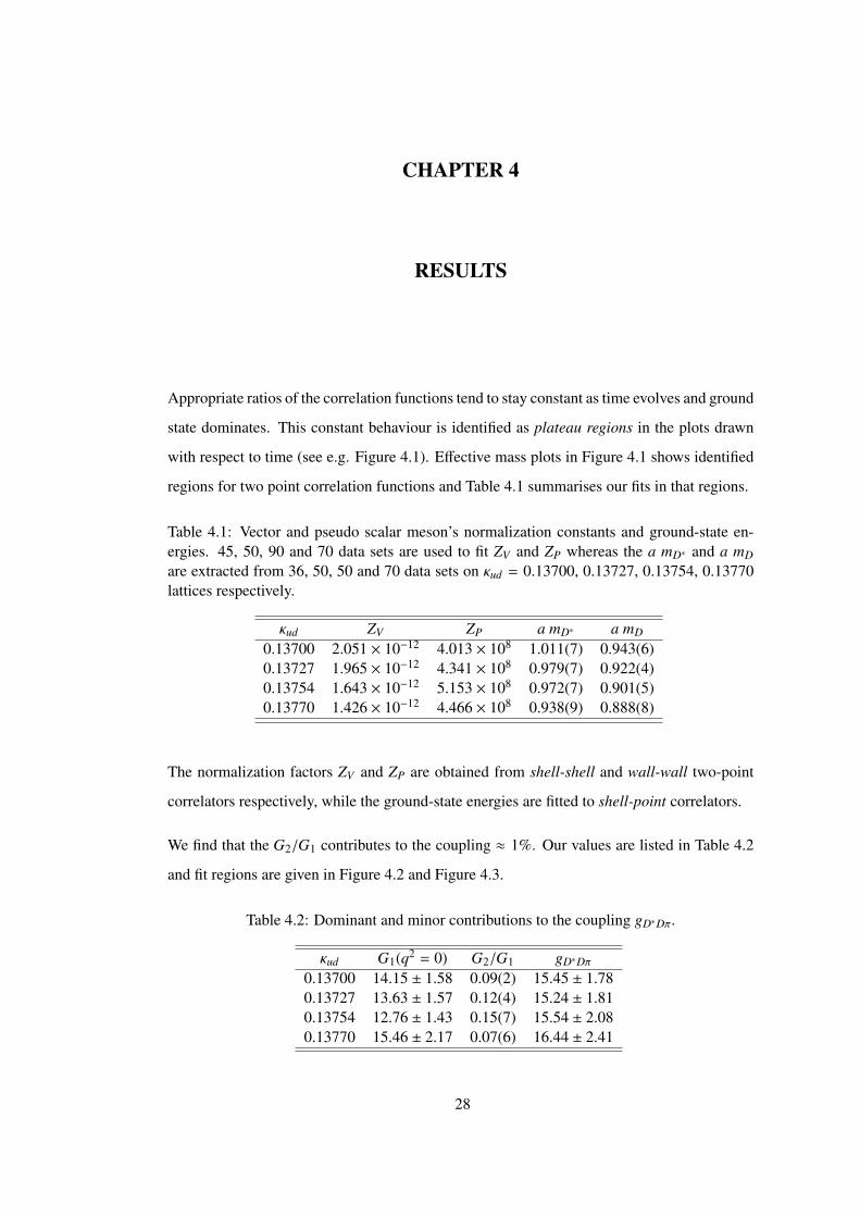
Appropriate ratios of the correlation functions tend to stay constant as time evolves and ground

state dominates. This constant behaviour is identified as plateau regions in the plots drawn

with respect to time (see e.g. Figure 4.1). Effective mass plots in Figure 4.1 shows identified

regions for two point correlation functions and Table 4.1 summarises our fits in that regions.

Table 4.1: Vector and pseudo scalar meson’s normalization constants and ground-state en-ergies. 45, 50, 90 and 70 data sets are used to fit ZV and ZP whereas the a mD∗ and a mD

are extracted from 36, 50, 50 and 70 data sets on κud = 0.13700, 0.13727, 0.13754, 0.13770lattices respectively.

κud ZV ZP a mD∗ a mD

0.13700 2.051 × 10−12 4.013 × 108 1.011(7) 0.943(6)0.13727 1.965 × 10−12 4.341 × 108 0.979(7) 0.922(4)0.13754 1.643 × 10−12 5.153 × 108 0.972(7) 0.901(5)0.13770 1.426 × 10−12 4.466 × 108 0.938(9) 0.888(8)

The normalization factors ZV and ZP are obtained from shell-shell and wall-wall two-point

correlators respectively, while the ground-state energies are fitted to shell-point correlators.

We find that the G2/G1 contributes to the coupling ≈ 1%. Our values are listed in Table 4.2

and fit regions are given in Figure 4.2 and Figure 4.3.

Table 4.2: Dominant and minor contributions to the coupling gD∗Dπ.

κud G1(q2 = 0) G2/G1 gD∗Dπ

0.13700 14.15 ± 1.58 0.09(2) 15.45 ± 1.780.13727 13.63 ± 1.57 0.12(4) 15.24 ± 1.810.13754 12.76 ± 1.43 0.15(7) 15.54 ± 2.080.13770 15.46 ± 2.17 0.07(6) 16.44 ± 2.41

28

4.1 Chiral Extrapolations

As we stated before, technical drawbacks force us to carry our simulations with unphysical

quark masses on lattices. In order to estimate the gD∗Dπ at the physical point we extrapolate

our results to the chiral point (i.e. mq → 0).

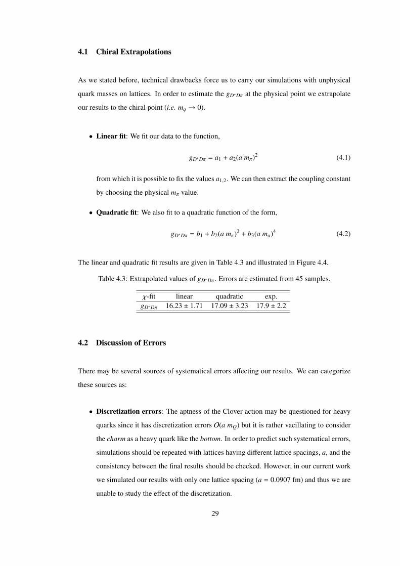
• Linear fit: We fit our data to the function,

gD∗Dπ = a1 + a2(a mπ)2 (4.1)

from which it is possible to fix the values a1,2. We can then extract the coupling constant

by choosing the physical mπ value.

• Quadratic fit: We also fit to a quadratic function of the form,

gD∗Dπ = b1 + b2(a mπ)2 + b3(a mπ)4 (4.2)

The linear and quadratic fit results are given in Table 4.3 and illustrated in Figure 4.4.

Table 4.3: Extrapolated values of gD∗Dπ. Errors are estimated from 45 samples.

χ-fit linear quadratic exp.gD∗Dπ 16.23 ± 1.71 17.09 ± 3.23 17.9 ± 2.2

4.2 Discussion of Errors

There may be several sources of systematical errors affecting our results. We can categorize

these sources as:

• Discretization errors: The aptness of the Clover action may be questioned for heavy

quarks since it has discretization errors O(a mQ) but it is rather vacillating to consider

the charm as a heavy quark like the bottom. In order to predict such systematical errors,

simulations should be repeated with lattices having different lattice spacings, a, and the

consistency between the final results should be checked. However, in our current work

we simulated our results with only one lattice spacing (a = 0.0907 fm) and thus we are

unable to study the effect of the discretization.

29

• Finite-volume effects: These lattice artefacts are caused since we model the infinite

space-time as a finite-size hypercube. In principle, finite volume effects are negligible

as long as mπL > 4. Considering we have mπL in the range 4.5 ≤ mπL ≤ 10 we assume

minimal effect. However it is dependent on the object that is created on the lattice and

one should check the effects of the finite volume by re-simulating the calculations on

different sized lattices. Since we have 323 × 64 lattices only we can not estimate the

finite size effects but the analysis in Ref. [17] suggests 6% of error for lattices smaller

than ours. We may expect to have less errors than they found but we won’t be reflecting

this error to our final results.

• Renormalization: We estimate the axial-vector current renormalization constant in a

perturbative way as mentioned in Section 3.3. Comparing to the approach for vector-

current renormalization [33] and estimated error of O(10)% in Ref. [35] we can expect

to have approximately same errors.

• Chiral extrapolation: We ignore the fit errors on parameters a1,2 and b1,2,3 since we

expect negligible errors compared to the overall statistical error. Regarding the smaller

errors, we choose to consider the linear extrapolation value as our result.

Apart from systematical errors there are also statistical errors related to the Monte Carlo

sampling of the observables or fitting to data. In order to estimate these errors we employ the

jackknife resampling method.

30

CHAPTER 5

CONCLUSION

In our work we have estimated the D∗Dπ coupling constant by employing the ab initio Lattice

QCD method.

Throughout the thesis we have discussed the discretization of the continuum QCD and in-

troduced the lattice theory relevant to this work in a naive and rather compact fashion. Es-

tablishing the theoretical foundations we have outlined the typical workflow and difficulties

of the numerical calculations. We have also studied the parameterization of the transition

matrix element, 〈P(p′)|Aµ|V(p, λ)〉, in order to extract the coupling from the matrix element

calculated by the proper combinations of the correlation functions computed on lattice. We

performed our simulations on 323 × 64 sized lattices with lattice spacing a = 0.0907(13) fm

(a−1 = 2.176(31)GeV) and 2+1 flavor dynamical quarks. The coupling is determined on four

different gauge configurations with κ(sea)ud = (0.13700, 0.13727, 0.13754, 0.13770) which cor-

respond to mπ ∼ (700, 570, 410, 300) MeV and with physical strange quark, κ(sea)s = 0.1364.

We estimate the pionic coupling of the ground state D-mesons, gD∗Dπ, as,

gD∗Dπ = 16.23 ± 1.71 g(exp)D∗Dπ = 17.9 ± 0.3 ± 1.9

which is in good agreement with the experiment. Our value is larger compared to the several

QCD Sum Rules results and consistent with the previous lattice estimation.

More precise measurements may be desirable but regarding the > 10% experimental error,

next logical step would be to estimate the systematical errors in a more subtle manner by re-

performing the simulations on different sized lattices or by computing the quark propagators

with improved Fermilab action [36], which is an improved version of the Clover action. Con-

sidering the resources we have however, it is not possible to estimate the systematical errors

31

in the near future; instead generalizing this study to extract the axial-vector form factors and

studying the vector form factors of the D-mesons would be more feasible.

32

REFERENCES

[1] S. Aoki, K.-I. Ishikawa, N. Ishizuka, T. Izubuchi, D. Kadoh, K. Kanaya, Y. Kuramashi,Y. Namekawa, M. Okawa, Y. Taniguchi, A. Ukawa, N. Ukita, and T. Yoshie, “2+1 flavorlattice QCD toward the physical point,” Phys. Rev. D, vol. 79, p. 034503, Feb 2009.

[2] R. G. Edwards and B. Joo, “The Chroma software system for lattice QCD,”Nucl.Phys.Proc.Suppl., vol. 140, p. 832, 2005.

[3] J. B. et al., “Review of Particle Physics,” Phys. Rev. D, vol. 86, p. 010001, 2012.

[4] B. Blossier, P. Boucaud, M. Brinet, F. De Soto, X. Du, et al., “The Strong runningcoupling at τ and Z0 mass scales from lattice QCD,” 2012.

[5] W. Wolfram, “Low energy QCD and physics of hadrons,” Technische UniverstatMunchen, Presented at the SNP School 2012 at Japan, 2010.

[6] M. Okamoto, “Full determination of the CKM matrix using recent results from latticeQCD,” PoS, vol. LAT2005, p. 013, 2006.

[7] D. Drechsel and T. Walcher, “Hadron structure at low Q2,” Rev. Mod. Phys., vol. 80,pp. 731–785, Jul 2008.

[8] M. A. Shifman, A. Vainshtein, and V. I. Zakharov, “QCD and Resonance Physics. SumRules,” Nucl.Phys., vol. B147, pp. 385–447, 1979.

[9] B. L. Ioffe, “QCD at Low Energies,” Prog.Part.Nucl.Phys., vol. 56, pp. 232–277, 2006.

[10] L. Reinders, H. Rubinstein, and S. Yazaki, “Hadron properties from QCD sum rules,”Physics Reports, vol. 127, no. 1, pp. 1 – 97, 1985.

[11] J. Gasser and H. Leutwyler, “Chiral Perturbation Theory: Expansions in the Mass of theStrange Quark,” Nucl.Phys., vol. B250, p. 465, 1985.

[12] S. Weinberg, “Phenomenological Lagrangians,” Physica, vol. A96, p. 327, 1979.

[13] Ph. Hagler, “Hadron structure from lattice quantum chromodynamics,” Physics Reports,vol. 490, no. 3-5, pp. 49 – 175, 2010.

[14] S. G. Matinyan and B. Muller, “A Model of charmonium absorption by light mesons,”Phys.Rev., vol. C58, pp. 2994–2997, 1998.

[15] S. Ahmed et al., “First measurement of Gamma(D*+),” Phys.Rev.Lett., vol. 87,p. 251801, 2001.

[16] F. Duraes, F. Navarra, M. Nielsen, and M. Robilotta, “Meson loops and the g(D*D pi)coupling,” Braz.J.Phys., vol. 36, pp. 1232–1237, 2006.

[17] A. Abada, D. Becirevic, P. Boucaud, G. Herdoiza, J. Leroy, et al., “First lattice QCDestimate of the gD∗Dπ coupling,” Phys.Rev., vol. D66, no. 074504, 2002.

33

[18] C. Gattringer and C. B. Lang, Quantum chromodynamics on the lattice, vol. 788. 2010.

[19] M. E. Peskin and D. V. Schroeder, An Introduction To Quantum Field Theory (Frontiersin Physics). Westview Press, 1995.

[20] K. G. Wilson, “Confinement of quarks,” Phys. Rev. D, vol. 10, pp. 2445–2459, Oct 1974.

[21] Y. Iwasaki, “Renormalization Group Analysis of Lattice Theories and Improved Lat-tice Action. II four-dimensional non-abelian SU(N) gauge model,” UTHEP-118 (un-published), 1983.

[22] M. Luscher and P. Weisz, “On-Shell Improved Lattice Gauge Theories,” Com-mun.Math.Phys., vol. 97, p. 59, 1985.

[23] B. Sheikholeslami and R. Wohlert, “Improved Continuum Limit Lattice Action for QCDwith Wilson Fermions,” Nucl.Phys., vol. B259, p. 572, 1985.

[24] H. Neuberger, “Exactly massless quarks on the lattice,” Phys.Lett., vol. B417, pp. 141–144, 1998.

[25] D. B. Kaplan, “A Method for simulating chiral fermions on the lattice,” Phys.Lett.,vol. B288, pp. 342–347, 1992.

[26] J. B. Kogut and L. Susskind, “Hamiltonian Formulation of Wilson’s Lattice Gauge The-ories,” Phys.Rev., vol. D11, p. 395, 1975.

[27] R. Frezzotti, S. Sint, and P. Weisz, “O(a) improved twisted mass lattice QCD,” JHEP,vol. 0107, p. 048, 2001.

[28] S. Aoki et al., “Comparative study of full QCD hadron spectrum and static quark poten-tial with improved actions,” Phys.Rev., vol. D60, p. 114508, 1999.

[29] S. Aoki et al., “Nonperturbative O(a) improvement of the Wilson quark action withthe RG-improved gauge action using the Schrodinger functional method,” Phys.Rev.,vol. D73, p. 034501, 2006.

[30] M. Gell-Mann and M. Levy, “The axial vector current in beta decay,” Nuovo Cim.,vol. 16, p. 705, 1960.

[31] Y. Nambu, “Axial Vector Current Conservation in Weak Interactions,” Phys. Rev. Lett.,vol. 4, pp. 380–382, Apr 1960.

[32] J. J. Sakurai, Currents and mesons. Chicago: University of Chicago Press, 1969.

[33] A. Ali Khan, S. Aoki, G. Boyd, R. Burkhalter, S. Ejiri, M. Fukugita, S. Hashimoto,N. Ishizuka, Y. Iwasaki, K. Kanaya, T. Kaneko, Y. Kuramashi, T. Manke, K. Nagai,M. Okawa, H. P. Shanahan, A. Ukawa, and T. Yoshie, “Light hadron spectroscopy withtwo flavors of dynamical quarks on the lattice,” Phys. Rev. D, vol. 65, p. 054505, Feb2002.

[34] W. Wilcox, T. Draper, and K.-F. Liu, “Chiral limit of nucleon lattice electromagneticform factors,” Phys. Rev. D, vol. 46, pp. 1109–1122, Aug 1992.

[35] G. Erkol, M. Oka, and T. T. Takahashi, “Axial Charges of Octet Baryons in Two-flavorLattice QCD,” Phys.Lett., vol. B686, pp. 36–40, 2010.

34

[36] M. B. Oktay and A. S. Kronfeld, “New lattice action for heavy quarks,” Phys.Rev.,vol. D78, p. 014504, 2008.

35

APPENDIX A

Ratio

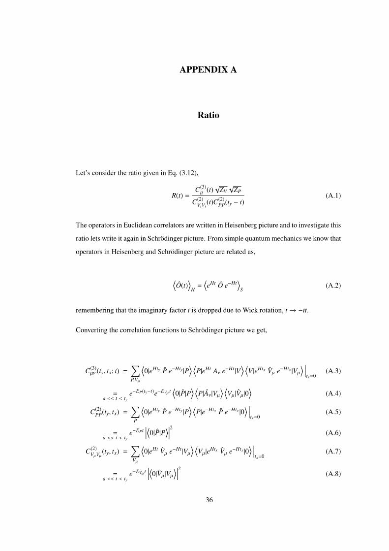
Let’s consider the ratio given in Eq. (3.12),

R(t) =C(3)

ii (t)√

ZV√

ZP

C(2)ViVi

(t)C(2)PP(ty − t)

(A.1)

The operators in Euclidean correlators are written in Heisenberg picture and to investigate this

ratio lets write it again in Schrodinger picture. From simple quantum mechanics we know that

operators in Heisenberg and Schrodinger picture are related as,

⟨O(t)

⟩H

=⟨eHt O e−Ht

⟩S

(A.2)

remembering that the imaginary factor i is dropped due to Wick rotation, t → −it.

Converting the correlation functions to Schrodinger picture we get,

C(3)µν (ty, tx; t) =

∑P,Vµ

⟨0|eHty P e−Hty |P

⟩ ⟨P|eHt Aν e−Ht|V

⟩ ⟨V |eHtx Vµ e−Htx |Vµ

⟩ ∣∣∣∣tx=0

(A.3)

=a << t < ty

e−EP(ty−t)e−EVµ t⟨0|P|P

⟩ ⟨P|Aν|Vµ

⟩ ⟨Vµ|Vµ|0

⟩(A.4)

C(2)PP(ty, tx) =

∑P

⟨0|eHty P e−Hty |P

⟩ ⟨P|e−Htx P e−Htx |0

⟩ ∣∣∣∣tx=0

(A.5)

=a << t < ty

e−EPt∣∣∣∣⟨0|P|P

⟩∣∣∣∣2 (A.6)

C(2)VµVµ

(ty, tx) =∑Vµ

⟨0|eHt Vµ e−Ht|Vµ

⟩ ⟨Vµ|eHtx Vµ e−Htx |0

⟩ ∣∣∣∣tx=0

(A.7)

=a << t < ty

e−EVµ t∣∣∣∣⟨0|Vµ|Vµ

⟩∣∣∣∣2 (A.8)

36

where we can identify the ZP =∣∣∣∣⟨0|P|P

⟩∣∣∣∣2 and ZV =∣∣∣∣⟨0|Vµ|Vµ

⟩∣∣∣∣2 from Eq. (3.13)

By putting ZP, ZV and Eqs. (A.4), (A.6), (A.8) into the Eq. (A.1) we see that it reduces to the

coupling,

R =⟨P|Aν|Vµ

⟩= gVPAµ (A.9)

37

APPENDIX B

Wall-Smearing Method

The three point correlation function can be written in terms of the quark propagators S (x, x′)

after the contractions specified by Wick’s Theorem,

〈CD∗AµD(t2, t1; p′,p)〉 = −i∑x2,x1

e−ip·x2eiq·x1 〈Tr[γµ S u(0, x1) γµγ5 S u(x1, x2) γ5 S c(x2, 0)]〉

(B.1)

While point-to-all propagators S u(0, x1) and S c(x2, 0) can be easily obtained, the computation

of all-to-all propagator S u(x1, x2) is a formidable task. One common method is to use a

sequential source composed of S u(0, x1) and S c(x2, 0) for the Dirac matrix and invert it in

order to compute S u(x1, x2) [34]. However, this method requires to fix either the inserted

current or the sink momentum.

An approach that does not require to fix any of the above is the wall-smearing method, where

a summation over the spatial sites at the sink time point, x2, is made before the inversion. This

corresponds to having a wall source or sink:

〈CD∗AµDS W (t2, t1; 0,p)〉 = −i

∑x2,x′2,x1

eiq·x1 〈Tr[γµ S u(0, x1) γµγ5 S u(x1, x′2) γ5 S c(x2, 0)]〉 (B.2)

where the propagator (instead of the hadron state) is projected on to definite momentum (S

and W are smearing labels for shell and wall). The wall method has the advantage that one can

first compute the shell and wall propagators and then contract these to obtain the three-point

correlator, avoiding any sequential inversions.

38

0 5 10 15 20

0.82

0.84

0.86

0.88

0.9

0.92

0.94

0.96

0.98

(!ud , !c)= (0.13700, 0.1224)(!ud , !c)= (0.13727, 0.1224)(!ud , !c)= (0.13754, 0.1224)

t

ln(

C(2

) (t)/

C(2

) (t+

1))

D - meson

(!ud , !c)= (0.13770, 0.1224)

0 5 10 15 20

0.85

0.9

0.95

1

1.05

1.1

(!ud , !c)= (0.13700, 0.1224)(!ud , !c)= (0.13727, 0.1224)(!ud , !c)= (0.13754, 0.1224)

t

ln(

C(2

) (t)/

C(2

) (t+

1))

D* - meson

(!ud , !c)= (0.13770, 0.1224)

Figure 4.1: Effective mass plots. Black horizontal lines indicate the fit regions.

39

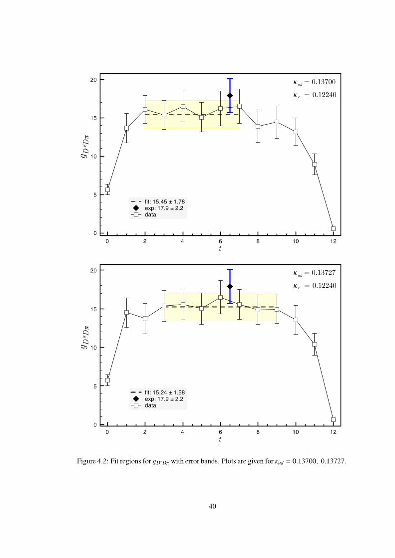
0 2 4 6 8 10 120

5

10

15

20

fit: 15.45 ± 1.78exp: 17.9 ± 2.2data

g D*Dπ

t

𝜅 = 0.13700𝜅 = 0.12240

ud

c

0 2 4 6 8 10 120

5

10

15

20

fit: 15.24 ± 1.58exp: 17.9 ± 2.2data

g D*Dπ

t

! = 0.13727! = 0.12240

ud

c

Figure 4.2: Fit regions for gD∗Dπ with error bands. Plots are given for κud = 0.13700, 0.13727.

40

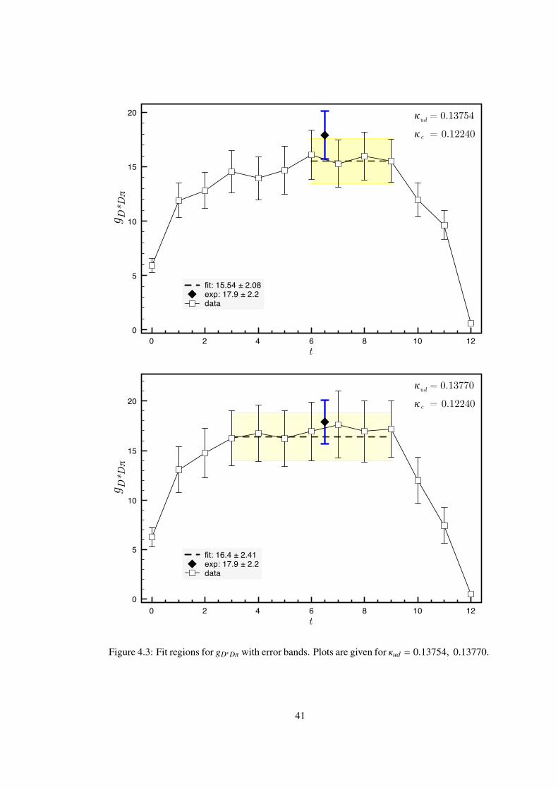
0 2 4 6 8 10 120

5

10

15

20

fit: 15.54 ± 2.08exp: 17.9 ± 2.2data

g D*Dπ

t

! = 0.13754! = 0.12240

ud

c

0 2 4 6 8 10 120

5

10

15

20

fit: 16.4 ± 2.41exp: 17.9 ± 2.2data

g D*Dπ

t

! = 0.13770! = 0.12240

ud

c

Figure 4.3: Fit regions for gD∗Dπ with error bands. Plots are given for κud = 0.13754, 0.13770.

41

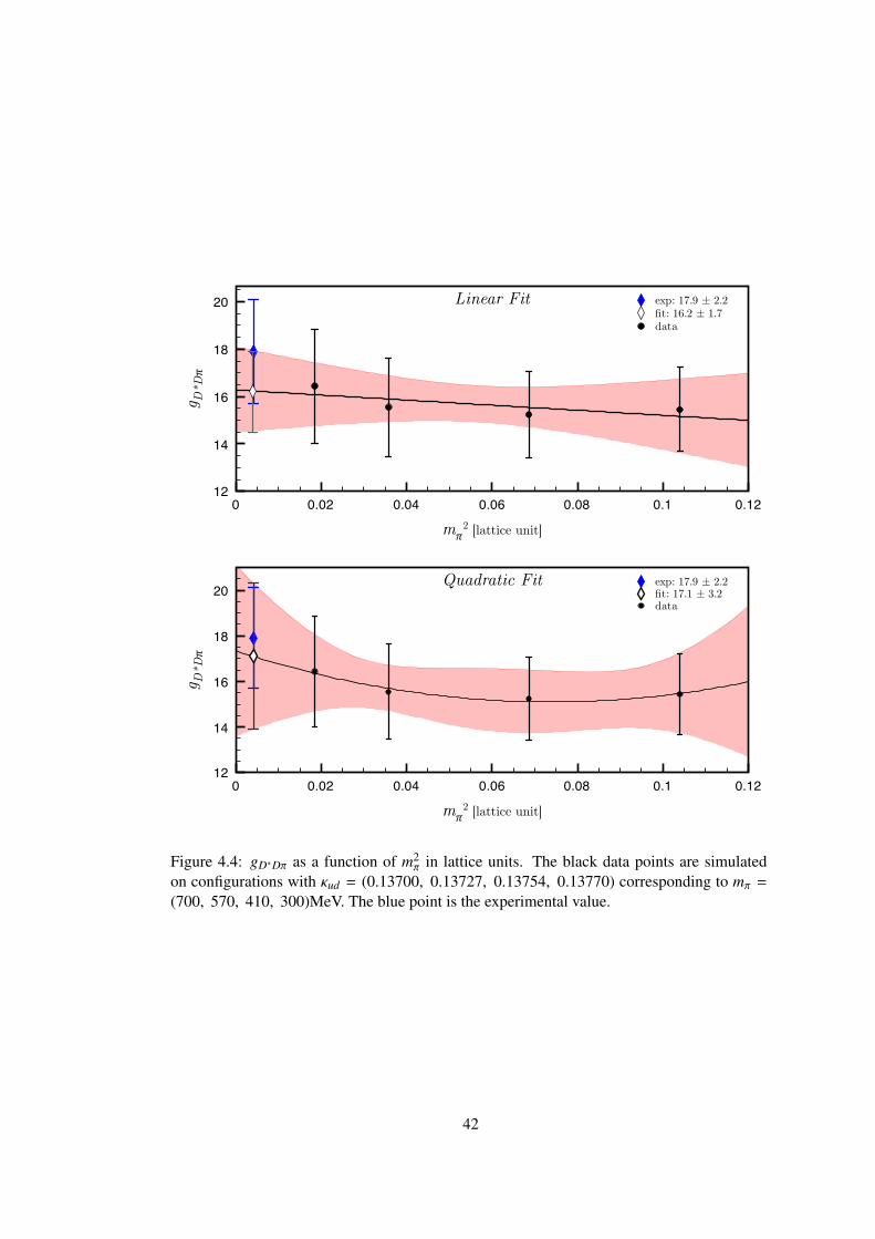
0 0.02 0.04 0.06 0.08 0.1 0.1212

14

16

18

20 exp: 17.9 ± 2.2fit: 16.2 ± 1.7data

m𝜋2 [lattice unit]

g D*D𝜋

Linear Fit

0 0.02 0.04 0.06 0.08 0.1 0.1212

14

16

18

20exp: 17.9 ± 2.2fit: 17.1 ± 3.2data

m𝜋2 [lattice unit]

g D*D𝜋

Quadratic Fit

Figure 4.4: gD∗Dπ as a function of m2π in lattice units. The black data points are simulated

on configurations with κud = (0.13700, 0.13727, 0.13754, 0.13770) corresponding to mπ =

(700, 570, 410, 300)MeV. The blue point is the experimental value.

42