DC Readout at the LIGO 40-meter Interferometer

Darcy Barron

Mentor: Sam Waldman

Abstract

Currently, Initial LIGO is using RF phase modulation of the input beam to encode

the output gravitational wave signal. The new DC readout scheme for Advanced LIGO

will use amplitude modulation of the main laser field as the gravitational wave signal.

This new method will eliminate several noise sources. The DC readout requires new in-

vacuum hardware, including a mode-matching telescope and an output mode cleaner.

The purpose of this project is to characterize the components of the DC readout

experiment at the LIGO 40-meter interferometer and install the setup in the vacuum

chamber of the interferometer for testing.

Introduction/Background

The LIGO project is attempting to detect gravitational waves, which are waves in space-

time predicted by general relativity. The LIGO detectors are Michelson interferometers, with

Fabry-Perot cavities in the arms to increase the light’s path length. The laser light goes through a

beam splitter and down two perpendicular arms to the Fabry-Perot cavities, and then returns to

the beam splitter. If the arms are the same length, or if the paths of the beams differ by an

integral number of wavelengths, the two light beams will interfere destructively and cancel each

other out, resulting in no light being detected at the asymmetric port. A gravitational wave

would cause a decrease in length along one direction and an increase in an orthogonal direction,

which would result in the arms having different lengths. This difference in length would cause a

difference in the phase of the light beams, and the beams would not completely cancel each other

out. This light is read as the gravitational wave signal.

Currently, initial LIGO is using an RF phase modulation of the input beam to create the

signal, with the gravitational wave signal encoded at the RF sideband frequency. LIGO DC

readout project is working on a new way to read the signal produced by gravitational waves,

which will be used for Advanced LIGO. A prototype has been built and is being tested at the

40m interferometer. The new DC readout will use amplitude modulation of the main laser field

as the gravitational wave signal. The RF sidebands and higher order modes of light are filtered

out before the light reaches the readout photodiode. Only the TEM00 mode of the carrier

frequency and the signal sidebands will pass through to the detector. This new method will

eliminate or reduce several noise sources. Removing the RF sidebands will remove RF phase

oscillator noise in the signal, and removing higher order modes will result in a cleaner signal.

Also, reducing the amount of light that reaches the photodetector will reduce shot noise.

First, I will discuss the components and layout of the DC readout scheme. The DC

readout requires new in-vacuum hardware, including a mode-matching telescope and an output

mode cleaner. The next section will discuss the characterization work on the components of DC

readout. Finally, I will discuss the preparation work completed for installation of the setup into

the vacuum chamber of the interferometer, and future work including the installation and

alignment into the vacuum chamber.

DC Readout Components and Layout

The light comes out of the interferometer to two alignment mirrors, to the mode-matching

telescope, into the output mode cleaner, then onto two DC photodiodes. The layout is illustrated

in Figure 1.

Figure 1. In-vacuum layout of DC readout

Alignment PZT Mirrors

Alignment with the interferometer’s output signal is done with two tip-tilt PZT mirrors to

adjust the beam position and angle.

Output Mode-Matching Telescope

A mode-matching telescope comes before the output mode cleaner to match the input

beam to the cavity resonant mode so that the beam waist is the correct size and in the correct

position. The output mode-matching telescope consists of two curved mirrors and two flat

mirrors. The first mirror has a radius of curvature of 618.4 mm, and the second mirror has a

radius of curvature of 150 mm, so that the telescope has 4:1 beam reduction. The second mirror

is mounted on a translational stage so that the distance between the mirrors can be adjusted for

focusing. The layout of the mode-matching telescope is shown in Figure 2.

Figure 2. Output mode-matching telescope.

Output Mode Cleaner

The output mode cleaner is a Fabry-Perot cavity that in resonance will only allow the

TEM00 mode of the carrier and the signal sidebands to pass through, and all other modes and

frequencies will not resonate and will be reflected. This reflected beam is monitored by a

photodiode. The output mode cleaner consists of four mirrors mounted in a copper block with

holes for the cavity drilled out. One of the mirrors is mounted on a PZT to adjust the length of

the cavity to resonance. The layout of the output mode cleaner is shown in Figure 3. The green

line indicates the transmitted beam, and the blue line is the reflected beam.

Figure 3. Output mode cleaner.

In-Air Setup

Initially, the layout was set up and aligned in air. Figure 4 shows a picture of the setup,

with the beam path drawn in. A smaller laser than the actual interferometer laser was used with

a long beam path to imitate the beam that will be coming from the interferometer.

Figure 4. In-air setup of DC readout.

Characterization of Components

After the layout was set up in air, the components could be tested and characterized, in

preparation for their installation into the vacuum chamber of the interferometer.

Alignment PZT mirrors

Mirror displacement

To determine the range and functionality of the tip-tilt PZT mirrors, the mirrors were

driven one at a time, and the linear displacement of the beam at a later point in the path was

measured. An angular displacement was calculated from the linear displacement, and this was

used to calculate the range of the PZT mirrors. A detailed description of the methods used can

be found in part 1 of the Methods section. The expected range of the mirrors was 4 mrads at the

full 160 V range, from -10 V to 150 V. Calculating the full range from the linear displacement at

a smaller voltage resulted in values of about 8 mrad for pitch and 11 mrad for yaw. There were

many errors in the values of distances, voltages, and other things that could have led to the

differences in the expected and measured values, but the measurements at least showed that the

PZT’s are functional. The reason for the difference in the range for pitch and yaw is not known.

Frequency Response

The frequency response of the PZT mirrors was measured using a frequency analyzer

(See Methods part 2). The frequency response, shown in Figure 5, showed good results, with a

flat response out to several hundred Hz.

Figure 5. Frequency response of tip-tilt PZT.

Strain Gauge

The PZT has a strain gauge to measure the physical strain of the PZT stacks. The strain

gauge voltage was measured and the differential voltage between the stacks was calculated from

the PZT drive voltage (See Methods part 3). The differential voltage plotted with the strain

gauge voltage shows a hysteresis loop as the differential voltage goes from positive to negative

and back to its starting point. The results are shown in Figure 6.

Figure 6. Strain gauge voltage versus differential voltage for alignment PZT.

Output Mode Cleaner

Finesse of Output Mode Cleaner

The finesse of the output mode cleaner was measured in two different ways (See Methods

part 4). The finesse is defined to be the free spectral range divided by the FWHM bandwidth of

the resonances1:

!

F ="#

ax

"#cav

Using the oscilloscope, a finesse of 192 was calculated. Using the data from the

oscilloscope in Matlab, a finesse of 175 and 156 was calculated. The two different values of

finesse are a result of two different values of the free spectral range that were measured in the

data.

FFT of output mode cleaner cavity

To lock the cavity, we set up an offset lock, using a photodiode after the output mode

cleaner to generate an error signal (See Methods part 5). An FFT of the error signal from the

OMC length control servo was done using a frequency analyzer, and it showed an unexplained

peak at about 456 Hz. Other peaks are resonances of the 60 Hz power lines. The FFT is shown

in Figure 7.

Figure 7. FFT of OMC.

Linear OMC PZT

Voltage Response

To measure the voltage response of the linear PZT in the output mode cleaner, the

voltage required to go from one resonance peak to another was measured. This voltage

corresponds to the PZT moving by a half wavelength. The wavelength of the laser is 1064 nm,

so the voltage response of the PZT is 8.3 nm/V.

Linearity of voltage response of OMC PZT

The linearity of the voltage response of the linear PZT was not certain, so a measurement

was designed to determine the voltage response at different voltages. The FWHM of the

resonance peak was calculated from data taken as the cavity was heated, creating a length offset

and changing the voltage that resonance occurred. (See Methods part 6). The results, shown in

Figure 8, show that the FWHM of the resonance peak of the OMC remained constant for all

drive voltages, so the voltage response is linear.

Figure 8. PZT drive voltage vs. FWHM for linear OMC PZT.

Linear OMC PZT Frequency Response

The PZT frequency response shown in Figure 9 was performed using a frequency

analyzer (see Methods part 2), and showed that the first resonance was at about 50 kHz.

Figure 9. Frequency response of linear PZT in OMC.

Losses in OMC

To measure the losses in the cavity, a power meter was used to measure the power of

light going into and out of the cavity when the cavity was locked and unlocked. The location of

the beams is shown in Figure 10.

Figure 10. Output mode cleaner beams.

The reflectivities of the mirrors and the power measurements were used to calculate the

transmission of the cavity and the loss per round trip. The equations used can be found in

Methods part 7. The power measurements and loss calculations are shown in Table I. Incident 42 mW Reflected 26 mW Input 16 mW Transmitted 15 mW Leak 120 µW Transmission 95% Loss per round trip 0.1% Background 0.5 µW

Table I. Power measurements of OMC.

Preparation for installation in vacuum

After the in-air setup had been aligned and characterized, all of the hardware was

disassembled. The pieces were then prepared to go in vacuum by cleaning them, which was

removing contaminants by either baking them or cleaning them with methanol. Once the pieces

were clean, they were reassembled in a clean room. The laser beam that had been used for the

in-air setup was split into two and coupled into two 50-meter fiber optic cables. The fibers ran

into the clean room to a fiber launch where the beams could be used to align the setup. The

setup was pre-aligned in the clean room using the two beams for a forward and a back

propagating beam.

Future Work

After the setup is pre-aligned in the vacuum, it will be ready to be installed into the

vacuum chamber of the interferometer. The two laser fibers will again be used to align the setup

with forward and back propagating light. The pre-aligned setup will be aligned with the signal-

recycling mirror to align with the signal beam from the interferometer. After this is

accomplished, the testing of the new readout system will begin.

Methods Appendix

1. Calculating Displacement of PZT Mirrors

First, a circuit was designed and built to drive one degree of freedom of the PZT

mirror from –5 to +5 volts. The circuit consisted of a non-inverting and an inverting op-amp,

shown in Figure 112.

Figure 11. Circuit to drive PZT.

The steering mirrors have tip-tilt Piezojena piezoelectric transducers (PZT). The PZT

mirror was driven in pitch and yaw separately for each mirror, with each half of the stack driven

separately, then both halves together. Each mirror had a red, white, and black wire for each axis.

The red wire was ground and the black and white wires were signal wires for Vout and -Vout.

The two PZT mirrors align the beam to go into the mode-matching telescope and the

output mode cleaner. The mode-matching telescope has a 4:1 angle increase. The reflected

beam from the output mode cleaner was sent to a CCD camera and displayed on a TV screen.

For pitch and yaw of each mirror, the mirror was driven from negative five to plus five volts and

the displacement on the screen was measured.

The TV screen was 14.2 centimeters by 11.3 centimeters, and the CCD was 0.8 centimeters by

0.6 centimeters.

Using ray matrices, the displacement of the beam at the CCD was converted into an angle

of the PZT mirror. Ray matrices are used to calculate the change in displacement and angle of a

beam after passing through optical elements.

1,

1

1

,

2

2

2Mr

r

r

DC

BA

r

rr =!

"

#$%

&'!"

#$%

&=!

"

#$%

&=

The ABCD matrix for a beam traveling through free space is

!"

#$%

&

10

1 L

The ABCD matrix for a beam incident on a curved mirror is

!"

#$%

&

' 1/2

01

R

The matrices for each element are multiplied, in reverse order of incidence, to obtain the

matrix M for the optical path3. Using the distances between optics and the radii of curvature of

the mirrors in the mode-matching telescope, a matrix was calculated for the optical paths. The

matrix for the path from the first alignment mirror to the CCD camera is

!

"0.29 "4.58

"0.048 "4.21

#

$ %

&

' (

The matrix for the path from the second alignment mirror to the CCD camera is

!

"0.29 "4.15

".048 "4.13

#

$ %

&

' (

Using the B values of these matrices, the conversion from angle to linear displacement

for the first mirror to the CCD is -4.58 meters/radian, and -4.15 meters/radian for the second

mirror. The values for displacement and angle and the calibration for radians/volt are shown in

Table II and Table III.

PZT 1 Pitch Displacement (cm) TV Screen CCD Angle (mrad) Rad/Volt Total Range (mrad)

Both 4.3 0.23 0.50 0.05 7.53 White Wire 1.9 0.1 0.23 0.023 3.27 Black Wire 1.9 0.1 0.22 0.022 3.27

PZT 1 Yaw Displacement (cm) TV Screen CCD Angle (mrad) Rad/Volt Total Range (mrad)

Both 5.5 0.31 0.68 0.068 10.15 White Wire 2.7 0.15 0.33 0.033 4.91 Black Wire 2.8 0.16 0.35 0.035 5.24

Table II. Displacement of beam at first PZT mirror, B=-4.58.

PZT 2 Pitch Displacement cm)

TV Screen CCD Angle (mrad) Rad/Volt Total range (mrad) Both 4 0.21 0.51 0.05 7.60

White wire 1.9 0.1 0.24 0.021 3.62 Black wire 1.9 0.1 0.24 0.024 3.62

PZT 2 Yaw displacement (cm)

TV Screen CCD Angle (mrad) Rad/Volt Total Range

(mrad) Both 5.5 0.31 0.75 0.077 11.22

White wire 2.5 0.14 0.34 0.034 5.07 Black wire 2.5 0.14 0.34 0.034 5.07

Table III. Displacement of beam at second PZT mirror, B=-4.15.

2. Frequency Response of PZT

To measure the frequency response of the PZT’s, clips were used to measure the voltage

at the PZT, then attached it to a 7 Hz high pass filter and then attached to the reference channel

of the frequency analyzer. A photodiode was connected to the other channel. A 200 Hz high pass

filter was connected to the source out, which went to the PZT driver and a power supply for an

offset. The PZT was driven in pitch and yaw separately for the tip-tilt PZT’s.

The frequency response of one of the PZT mirrors showed a large peak around 80 Hz

when driven only in yaw. When the peak was investigated, it was shown that the mirror was

moving in pitch while being driven only in yaw at a certain frequency. The PZT was taken apart,

and it was found that one of the stacks was loose, so it was sent in for repair.

3. Strain Gauge of PZT

The circuit for the strain gauge is a Wheatstone bridge, which measures a resistance

change4. The voltage of the strain gauge in the PZT was measured by connecting the strain

gauge to a power supply and connecting it to an oscilloscope. The voltage was 2 V with a 104

gain. The strain gauge had 4 wires that were red, black, white, and green. The red and green

were opposite sides of the bridge, as were the black and white. A signal generator with a 1 V

triangle wave was connected to the PZT driver for a drive voltage. The differential voltage,

which was the difference in voltage going to the two signal wires, was determined by changing

the drive voltage and measuring the voltage on the signal wires using an oscilloscope probe. The

conversion was linear, and was calculated to be

Differential=Drive*59.5-2.55

4. Finesse of Output Mode Cleaner

To measure the finesse of the output mode cleaner cavity, a frequency generator was used

to produce a triangle wave that was sent to the PZT driver with sufficient amplitude to sweep

across fringes of the cavity.

The oscilloscope was used to measure the full width at half maximum (FWHM) of the

resonance peak and the free spectral range (FSR) between peaks by viewing the voltage on the

screen and using cursors. Data from the oscilloscope was recorded over 5 resonance peaks and 2

free spectral ranges.

Using the data from the oscilloscope in Matlab, a Lorentzian curve was fit to each peak.

A Lorentzian is the function

22 )2

1()(

2

1

1

!+"

!

=

oxx

L#

where x0 is the center position and Γ is the full width at half maximum5.

One of the Lorentzian fits is shown in Figure 12.

Figure 12. Lorentzian fit of resonance peak.

A program was written to determine the FWHM and center position of peaks, average

the FWHM of five peaks and calculate the finesse using each value of the FSR.

5. Locking the output mode cleaner

The output mode cleaner cavity could be locked using a photodiode signal from the

transmitted beam or the leaking beam from the end of the cavity. For an offset lock, the signal

from the photodiode first had an offset added with a power supply, then was sent through a 1/20

voltage divider before going into a preamplifier to invert it, add gain of 200, and pass it through a

0.03 Hz low-pass filter. This signal was then sent back to the PZT driver. A function generator

was used to generate a sine wave to sweep the cavity through resonance, and the voltage offset

on the photodiode signal was adjusted so that the signal was zero when the cavity was on

resonance. The OMC was also dither-locked using a SR-785 lock-in amplifier.

6. Linearity of OMC Linear PZT Frequency Response

A frequency generator was connected to the PZT driver to drive across the full range of

the PZT with a triangle wave. A lamp was used to shine on the output mode cleaner to slowly

increase the temperature, expanding the cavity and acting as a voltage offset. The peaks were

measured as they moved through the voltage from the heating of the cavity. Using Matlab to

find the center of the peak and fit a Lorentzian curve to it, the FWHM of each peak was

determined. If the voltage response were linear, the FWHM would remain constant, as was the

case for this experiment.

7. Calculating losses in output mode cleaner.

The first measurement showed a transmission of the locked cavity of about sixty percent,

and a calculated loss per round trip of about 0.5 percent. Using the infrared viewer, the cavity

was examined, and light was seen scattering off the end with the PZT mounted mirror. The

mirror was slightly off center on its circular mount, so light was scattering off the misaligned

mirror. The mirror was unmounted, realigned to have the mirror be off center in the vertical

axis, and reglued. The cavity’s two input mirrors and the two alignment mirrors to the telescope

were adjusted to realign the cavity.

With the new alignment, the measurements with the power meter were repeated, and

showed much better transmission of about 94%. The values are shown in Table I.

Locked cavity Initial After realignment Incident 46 mW 42 mW Reflected 25 mW 26 mW Input 21 mW 16 mW Transmitted 12 mW 15 mW Leak 20 µW 120 µW Transmission 60% 94% Calc. loss per round trip 0.5% 0.1% Background: 0.5 µW

Table IV. Measurement of power and losses before and after realignment.

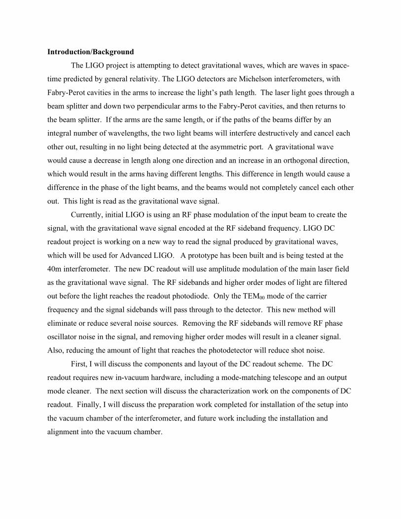
The following equations were used to calculate losses in the output mode cleaner using data from

the power meter and the finesse of the cavity.

R

1ln=! mirror coupling coefficient

210!!!! ++=

c total cavity loss factor

RF

1ln2

20

!="

# loss per round trip

2)1( RI

I

incident

dtransmitte != unlocked cavity

2

214

cincident

dtransmitte

I

I

!

!!" locked cavity

c

F!

"2= finesse of cavity

12

2

4

1exp

!

""

#

$

%%

&

'

((

)

*

++

,

-

(()

*++,

-()

*+,

-()

*+,

-=

incident

dtransmitte

I

I

FR

. reflectivity of mirror6

References 1 Siegman, Anthony E. Lasers. University Science Books, 1986. Page 436. 2 Hill, Winfield, and Paul Horowitz. Art of Electronics. Cambridge University Press, 1980. Pages 4-95 3 Siegman 581-586, 593-597. 4 Hill and Horowitz 602.

5 Weisstein, Eric W. "Lorentzian Function." From MathWorld--A Wolfram Web Resource. http://mathworld.wolfram.com/LorentzianFunction.html

6 Siegman 428-431. Waldman, Sam. Mini lectures and discussions about DC readout including Fabry-Perot cavities, mode cleaners, mode matching, PZT’s. Ward, Rob. Mini lectures and discussions about DC readout. Weinstein, Alan. Mini lectures and discussions about LIGO. Acknowledgements Thanks to Sam Waldman, Rob Ward, Alan Weinstein, Ken Libbrecht, and the 40-meter lab for their help, and thanks to LIGO and NSF for their support.