dbms metrology: measuring query timerts/pubs/a3-currim.pdf · 2019-10-28 · 3 dbms metrology:...

3

DBMS Metrology: Measuring Query Time

SABAH CURRIM, RICHARD T. SNODGRASS, YOUNG-KYOON SUH,and RUI ZHANG, University of Arizona

It is surprisingly hard to obtain accurate and precise measurements of the time spent executing a querybecause there are many sources of variance. To understand these sources, we review relevant per-processand overall measures obtainable from the Linux kernel and introduce a structural causal model relatingthese measures. A thorough correlational analysis provides strong support for this model. We attempted todetermine why a particular measurement wasn’t repeatable and then to devise ways to eliminate or reducethat variance. This enabled us to articulate a timing protocol that applies to proprietary DBMSes, thatensures the repeatability of a query, and that obtains a quite accurate query execution time while droppingvery few outliers. This resulting query time measurement procedure, termed the Tucson Timing ProtocolVersion 2 (TTPv2), consists of the following steps: (i) perform sanity checks to ensure data validity; (ii) dropsome query executions via clearly motivated predicates; (iii) drop some entire queries at a cardinality,again via clearly motivated predicates; (iv) for those that remain, compute a single measured time by acarefully justified formula over the underlying measures of the remaining query executions; and (v) performpost-analysis sanity checks. The result is a mature, general, robust, self-checking protocol that providesa more precise and more accurate timing of the query. The protocol is also applicable to other operatingdomains in which measurements of multiple processes each doing computation and I/O is needed.

CCS Concepts: � Information systems → Database query processing; � Software and itsengineering → Software performance;

Additional Key Words and Phrases: Accuracy, database ergalics, repeatability, Tucson timing protocol

ACM Reference Format:Sabah Currim, Richard T. Snodgrass, Young-Kyoon Suh, and Rui Zhang. 2016. DBMS metrology: Measuringquery time. ACM Trans. Database Syst. 42, 1, Article 3 (November 2016), 42 pages.DOI: http://dx.doi.org/10.1145/2996454

1. INTRODUCTION

A common approach for at least the past 40 years to measure Database ManagementSystem (DBMS) query time is as follows.

“We used the UNIX time command to measure the elapsed time and CPU time. Allqueries were run 10 times. The resultant CPU usage was averaged.” H.-Y. Hwangand Y.-T. Yu [1987]Consider the measured times in Table I for a single query repeated 10 times, for which

considerable care (to be described in detail later) was taken to get repeatable resultsand for which many sources of time variation (also to be discussed) were eliminated.

This research has been supported in part by NSF grants IIS-0415101, IIS-0639106, CNS-0838948,IIS-1016205, and EIA-0080123, and by partial support from a grant from Microsoft Corporation.Authors’ addresses: S. Currim, Alumni Office, University of Arizona; email: [email protected];R. T. Snodgrass, Department of Computer Science, University of Arizona; email: [email protected];Y.-K. Suh, (corresponding author, current address) Korea Institute of Science and Technology Information(KISTI); email: [email protected]; R. Zhang, (current address) Dataware Ventures; email: [email protected] to make digital or hard copies of part or all of this work for personal or classroom use is grantedwithout fee provided that copies are not made or distributed for profit or commercial advantage and thatcopies show this notice on the first page or initial screen of a display along with the full citation. Copyrights forcomponents of this work owned by others than ACM must be honored. Abstracting with credit is permitted.To copy otherwise, to republish, to post on servers, to redistribute to lists, or to use any component of thiswork in other works requires prior specific permission and/or a fee. Permissions may be requested fromPublications Dept., ACM, Inc., 2 Penn Plaza, Suite 701, New York, NY 10121-0701 USA, fax +1 (212)869-0481, or [email protected]© 2016 ACM 0362-5915/2016/11-ART3 $15.00DOI: http://dx.doi.org/10.1145/2996454

ACM Transactions on Database Systems, Vol. 42, No. 1, Article 3, Publication date: November 2016.

http://dx.doi.org/10.1145/2996454

http://dx.doi.org/10.1145/2996454

3:2 S. Currim et al.

Table I. Measured Time of 10 Executions of a Query

1 2 3 4 5 6 7 8 9 10 Avg Std DevT imemeas 9321 9210 9964 13442 9310 9470 9206 9394 9280 9398 9800 1298(msec)

Even after taking those many proactive steps to improve the measurements, they stillvary quite a lot, from 9,206msec to 13,442msec (with the lowest and highest numbersin bold), a range of 4,236msec, which is more than 30% of the highest time. As we willsee, this variability arises from necessary daemon processes and their I/O and otherinteractions with the DBMS.

The accuracy of any measurement system is the “closeness of agreement betweena measured quantity value and a true quantity value of a measurand,” whereas theprecision of that system is the “closeness of agreement between . . . measured quan-tity values obtained by replicate measurements on the same or similar objects underspecified conditions” [Working Group 2 of the Joint Committee for Guides in Metrol-ogy (JCGM/WG 2) 2008]. (In some contexts, accuracy is termed external validity andprecision, repeatability.)

In the following, we address the central question just raised: How can we achieve(more) precise and accurate measurements of query execution time? In considering theapproach that is the norm, averaging 10 runs, one asks, why average? (The average,while statistically well-founded, makes assumptions about the extraneous factors; wewill look much more deeply into these factors.) In fact, why not minimum? (Using theminimum assumes that all variations due to extraneous factors are additive; we willshow that this is not the case.) Should all 10 times be used? (We will show that someexecutions are outliers for quite specific reasons and so should be dropped. We will thenbetter motivate using 19 executions.) If some are dropped, how many should remain?(We will provide a detailed rationale for dropping executions with specific properties.)Could additional information from the operating system help? (We will identify whichinformation is useful in refining the determination of query processing time.)

We previously proposed a structural causal model and timing protocol [S. Currimet al. 2013], which we term the Tucson Timing Protocol Version 1 (TTPv1). The mainlimitation of that protocol is that it dropped about 20% of the timings because ofphantom processes, those whose presence the protocol could detect but could not collecttheir measures. The longer the query ran, the higher the chance of a phantom process,thus effectively limiting the protocol to fast and moderately fast queries and biasingthe resulting measurements to such queries.

This article presents a refined protocol, Tucson Timing Protocol Version 2 (TTPv2),that (a) drops many fewer query executions, (b) adds many more sanity checks, (c) isbased on an elaborated structural causal model, and (d) estimates process I/O in a moresophisticated manner, thereby providing a more comprehensive, robust, defensiblemeasurement of query evaluation time and of process time generally.

The protocol chooses the median query time across the repeated query executionsfor several reasons that we articulate in Section 8.5. As an example, examine queryexecution #4 in Table I. That one query execution raises the average to above all nineother executions. The median of 9,357 is not affected by that one skewed value.

In this article, we address both accuracy and precision in detail, along the way de-veloping a comprehensive, carefully motivated query time measurement protocol. Thisprotocol is much more accurate, given that it retains 96% of the query measurements,as compared with 76% for TTPv1, and more than doubles the number of sanity checks.(We emphasize that we do not have ground truth and so are only stating that by notthrowing away some of the longer running measured queries, the refined protocol re-moves some of the systematic bias of the original protocol.) The refined protocol is also


DBMS Metrology: Measuring Query Time 3:3

Fig. 1. DBMS time taxonomy.

more precise, with a relative error for time measured of 2.3% and of time calculated of2.1%, as compared to 4.5% and 2.2% for TTPv1.

In the next section, we provide a taxonomy of time measurements. Section 3 considersmany subtle aspects of measuring time: mitigating disk, main memory, and DBMScache effects; ensuring data and plan repeatability; contending with O/S daemons;utilizing the wide range of Linux per-process and overall measures; and understandingthe intricacies of time measurement resolution. We then present a comprehensivestructural causal model for how the measures relate and test this model, finding thatit is strongly supported by the experimental results. Section 7 first looks at the way wecollect the measures and how we ensure that we haven’t missed any process; it thenexamines in detail the most complex part, that of computing the I/O time used by theDBMS. (Interestingly, Linux provides no direct measure of this highly relevant aspect,and even indirect approaches are quite complex.) We present the protocol in detail,emphasizing the many sanity checks along the way. Section 10 evaluates our approachagainst the existing protocol, showing that it is more precise and accurate. We end witha summary and an examination of future work.

2. BACKGROUND

There is a spectrum of granularities with regard to what is being measured and howit is measured, as summarized in the taxonomy shown in Figure 1 (with the darkerblocks being measured by our protocol). (We note in passing that there are alternativesto the root node of this tree, Query Time, such as DBMS startup time and queryplanning time. We don’t consider those further.) The first decision is whether to considertime as an independent variable (i.e., specified when the experiment is run) or as adependent variable (i.e., measured). The TPC-C benchmark is run for a user-specifiedlength of time (minutes to hours), along with the transaction mix (ratio of read andupdate transactions), and the number of completed transactions is measured, yieldinga measured transactions per minute [TPC 2010b]. We focus in this article on measuredquery time (i.e., as a dependent variable).



The second decision is to determine what is to be measured. This could be a mix oftransactions, each with one or more queries and updates, or a single transaction, or asingle SQL statement (query, insert, delete, or update). We focus here on measuringthe total time of a single query. Some of these measurements could also be made ofdatabases in which the queries are run over many distributed computers, say in thecloud [B. F. Cooper et al. 2010], or, at a smaller scale, on a local distributed system[R. F. Forman et al. 2001].

When measuring how much time an individual query running on a single serverrequires, one can look again at wall-clock time, which will include all the DBMSpro-cess(es), including those not actually evaluating the query, as well as operating systemdaemons and processes invoked by other users. The TPC-H benchmark [TPC 2010a]runs a host of queries over a prescribed database and measures total time for each, as dothe XBench [B. B. Yao et al. 2004] and τBench [S. W. Thomas et al. 2014] benchmarks.Or, one can look more closely, restricting oneself to just those DBMSprocesses actuallyexecuting the query or even to the time required for JDBC interaction, CPU execution,I/O, or network. One can measure I/O time or obtain counts, such as the number ofblocks read or written, perhaps differentiating between random and sequential diskI/O. One could also study the pattern of accesses, including differentiating synchronousfrom asynchronous I/O. For computation, one can also measure time or counts (such asnumber of CPU ticks). The same differentiation applies to measuring network activity.JDBC activity is generally composed of network activity (if the SQL statement initiatoris running off-server) and computation. Finally, one can delve into the specifics of theCPU performance of a DBMS, examining, for example, processor cache effects [A. G.Ailamaki et al. 1999] using profiling tools like Valgrind Developers [2010], which pro-vide instruction and cache hit metrics. Counts are generally collected either throughthe operating system or instrumented DBMS [R. Zhang et al. 2012] or by running adisk or cache simulation on the instrumented DBMS. Because they are gathered usingdifferent approaches, counts and time measurements can be compared to ensure thatthey consistent.

There are two types of overall time (the left-most measure in Figure 1, as contrastedwith the component times to the right: JDBC, CPU, I/O, and Network). The ProcessTime (PT) is defined as the sum of CPU, I/O, JDBC, and Network time. The querytime of interest here is the PT of the query process. The time difference between thestart and the completion of the process is called Elapsed Wall-clock Time (ET). Table Iprovides ET, which is by its very nature highly variable because of all the other thingsgoing on while the query executes.

This article will consider how to more accurately and precisely measure the timerequired to execute a single SQL statement, examining (a) overall ET, (b) overall DBMSPT (c) CPU time, and (d) I/O time. For understanding DBMS behavior, wall-clock time ishighly variable due to extraneous operating system daemons and user processes, whichis why we focus here on the harder problem: Finer grained measurements of DBMS PTand its CPU and I/O components. (Doing so can then provide insight into the additiveeffect of daemons and user processes.) We will extract counts from the operating systembut because we are measuring proprietary DBMSes, we will not consider approachesthat require that the DBMS itself be instrumented. Thus, we do not consider CPUor I/O simulation to obtain detailed counts and measures of cache performance nor ofrandom versus sequential I/O (we will consider overall I/O time). We do not focus onmeasuring network time; instead, we reduce network time to the absolute minimumby mounting the disks on the server (not using a network file server). We minimizeJDBC activity by returning a minimal result.

We show that it is possible to deduce DBMS query process I/O and computation times,which when summed provide a much more stable measure of DBMS processing than



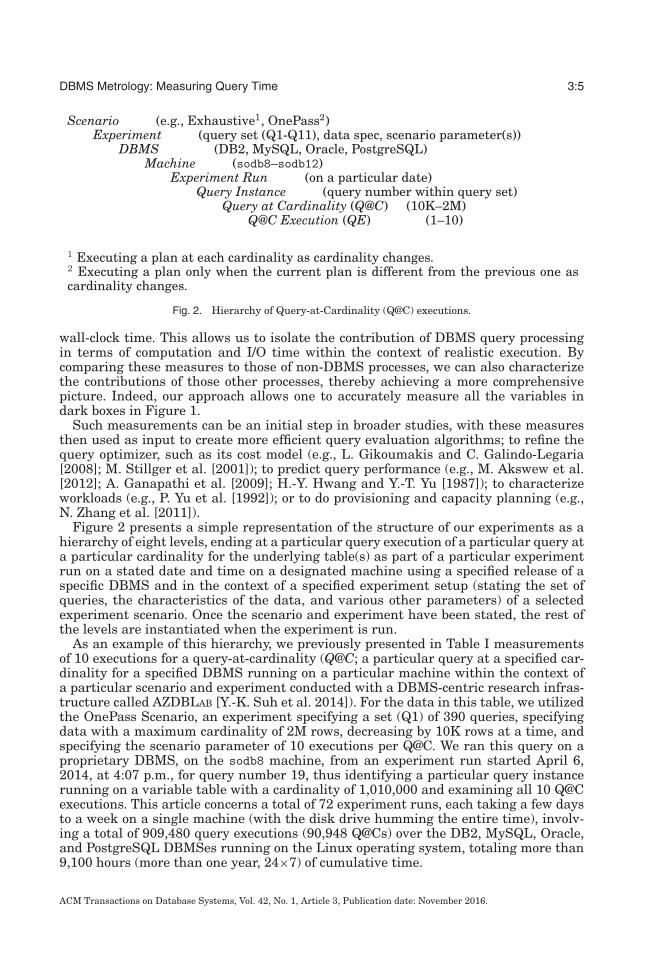
Fig. 2. Hierarchy of Query-at-Cardinality (Q@C) executions.

wall-clock time. This allows us to isolate the contribution of DBMS query processingin terms of computation and I/O time within the context of realistic execution. Bycomparing these measures to those of non-DBMS processes, we can also characterizethe contributions of those other processes, thereby achieving a more comprehensivepicture. Indeed, our approach allows one to accurately measure all the variables indark boxes in Figure 1.

Such measurements can be an initial step in broader studies, with these measuresthen used as input to create more efficient query evaluation algorithms; to refine thequery optimizer, such as its cost model (e.g., L. Gikoumakis and C. Galindo-Legaria[2008]; M. Stillger et al. [2001]); to predict query performance (e.g., M. Akswew et al.[2012]; A. Ganapathi et al. [2009]; H.-Y. Hwang and Y.-T. Yu [1987]); to characterizeworkloads (e.g., P. Yu et al. [1992]); or to do provisioning and capacity planning (e.g.,N. Zhang et al. [2011]).

Figure 2 presents a simple representation of the structure of our experiments as ahierarchy of eight levels, ending at a particular query execution of a particular query ata particular cardinality for the underlying table(s) as part of a particular experimentrun on a stated date and time on a designated machine using a specified release of aspecific DBMS and in the context of a specified experiment setup (stating the set ofqueries, the characteristics of the data, and various other parameters) of a selectedexperiment scenario. Once the scenario and experiment have been stated, the rest ofthe levels are instantiated when the experiment is run.

As an example of this hierarchy, we previously presented in Table I measurementsof 10 executions for a query-at-cardinality (Q@C; a particular query at a specified car-dinality for a specified DBMS running on a particular machine within the context ofa particular scenario and experiment conducted with a DBMS-centric research infras-tructure called AZDBLAB [Y.-K. Suh et al. 2014]). For the data in this table, we utilizedthe OnePass Scenario, an experiment specifying a set (Q1) of 390 queries, specifyingdata with a maximum cardinality of 2M rows, decreasing by 10K rows at a time, andspecifying the scenario parameter of 10 executions per Q@C. We ran this query on aproprietary DBMS, on the sodb8 machine, from an experiment run started April 6,2014, at 4:07 p.m., for query number 19, thus identifying a particular query instancerunning on a variable table with a cardinality of 1,010,000 and examining all 10 Q@Cexecutions. This article concerns a total of 72 experiment runs, each taking a few daysto a week on a single machine (with the disk drive humming the entire time), involv-ing a total of 909,480 query executions (90,948 Q@Cs) over the DB2, MySQL, Oracle,and PostgreSQL DBMSes running on the Linux operating system, totaling more than9,100 hours (more than one year, 24×7) of cumulative time.



Table II. Adjusting Number of QEs per Q@C

Number of Original QEs Percentage Dropped Number of Q@Cs Dropped Number of QEs Retained10 3.97% 2,207/55,585 9.59 4.55% 2,531/55,585 8.58 5.86% 3,260/55,585 7.67 10.31% 5,731/55,585 6.6

3. MEASURING QUERY TIME

We now turn our attention to the central problem: Measuring in a defensible mannerthe execution of a Q@C. These considerations inform the development of our protocol.

As we will see shortly, there are many other activities in addition to the strict querytime that is the focus here. Once a more precise and accurate query time is determined,those other aspects can also be measured either separately or in conjunction with thequery (say, by introducing them individually). In that way, the full context and scopeof a query can be quantified.

We execute in quick order, for a single query at a single cardinality, a certain numberof Q@C executions (also termed QEs). In our protocol, we execute each Q@C 10 times,which is sufficient for timing purposes. As we’ll see, Step 3-(iv) of the protocol, discussedin Section 8.4, drops Q@Cs with fewer than six QEs after many checks on these exe-cutions. (Why six QEs? Because that is the smallest sample size for which means andstandard deviations make sense.) This step retained about 96% of the Q@Cs, indicatingthat 10 is about the right number of QEs to start with. But this number of original QEsper each Q@C is a knob available to the experimenter. Table II shows the relationshipthat we observed between the number of original QEs, the number of Q@Cs droppedbecause they went below the threshold of six QEs after the protocol was applied, thenumber of Q@Cs actually dropped, and, finally, for the remaining Q@Cs, how manyQEs each retained on average. It seems that, for many situations, eight QEs per Q@Cwould work fine.

From various low-level measurements gathered during these remaining multipleexecutions, we then compute a QE time for that Q@C.

3.1. Cache Effects

Query evaluation normally involves intensive disk I/O, and so disk reads figure heavilyin timings. However, if the DBMS cache is warm, say because a previous query read indata pages that are part of the next query, then those data pages in main memory willnot need to be read back in, reducing overall I/O time.

If the DBMS main memory buffer is large enough to hold all the base tables andintermediate results, then the second time the same query is run, there should be noI/O at all. This can be termed pure warm cache. (As we will see, there are still issues indoing such timings, but at least no I/O is involved to complicate the timing further.) Ifthe DBMS main memory cannot hold everything, then there may be some I/O requiredto evaluate the query, depending on the details of the DBMS and file system cachemanager, which we term partial warm cache.

A further complication is that there are multiple caches involved: (a) most disk driveshave a several-MB cache; (b) many disk controllers also have a cache, which is typicallylarger than the disk cache; (c) the network file server generally has a large cache inmain memory; (d) the operating system the DBMS runs on has a large cache in mainmemory; (e) the DBMS buffer is generally large; (f) the JDBC driver may have a cache;and (g) the processor has a medium-sized L2 and a smaller L1 cache. We won’t considerthe processor L2 and L1 caches nor the JDBC cache further because they are generallyutilized in both warm and cold cache situations.



We focus in this article on the cold cache scenario because that is the most challeng-ing, although of course our protocol can also be used to measure warm cache scenarios.(Many other DBMS papers mention cold-cache measurements. We discuss the detailsfor two reasons: To be explicit on exactly how cold cache measurements can be doneand to enable discussion of the efficacy [accuracy and precision] of our protocol.)

We eliminate the caching and buffering artifacts via four general steps.First, we eliminated the problem of network file system caches by installing the disk

directly on the machine that also runs the DBMS. For the other caches, we consideredthe Linux hdparm -W command, which allows the drive’s write-caching feature to be set;the -f flag flushes the buffer cache. Note, however, that this feature only works on somedrives. Instead, we filled both the disk and disk controller caches by reading a 64MBdata file. The size of the data file was chosen so that it is bigger than the hard drivebuffer, which is 32MB. Third, we flushed the OS-related caches by using the Linuxdrop_caches facility to discard cached clean pages from the O/S file cache. Because nodirty pages would be created during QE, clearing the clean pages is sufficient.

We verified that these three steps were sufficient by timing the repeated readingof another file. Before the caches were flushed, the second read would take a muchshorter time than the first read. After the cache was flushed, the second read tookalmost exactly the same time (modulo other timing variations, to be discussed shortly)as the first read.

Fourth, we cleared the DBMS buffer via the provided API to discard cached con-tent residing inside the DBMS. (In some cases, there were multiple caches to becleared in the DBMS, each with a different kind of command. These caches wereoften not clearly documented; the commands were also sometimes hard to find.) ForDB2, it is necessary to deactivate the DBMS cache for the research database withsudo /opt/ibm/db2/v9.7/bin/db2 deactivate database research followed by a sim-ilar activate database research. For Oracle, the SQL command is ALTER SYSTEMFLUSH BUFFER_CACHE followed by ALTER SYSTEM FLUSH SHARED_POOL followed by ALTERSYSTEM CHECKPOINT. For MySQL the command is simply FLUSH TABLES. PostgreSQLsupports no such mechanism to clear all of its caches. PostgreSQL has two kinds ofcaches: shared_buffer (default 24MB, depending on the shmmax parameter under thekernel) and work_mem (default 1MB). The only way to clear these buffers is by restart-ing PostgreSQL. That said, because the shared buffer is so small, the effect of a warmcache on that DBMS is minimal.

There is an important philosophical point to be made here, one with implicationsin practice. Flushing the buffer cache may do other things, like close tables or resetother data structures. Doing so may require that tables be opened when the queryis (re-)executed and so can include components that were not in the original query.Thus, by flushing, our approach is made more precise (repeatable, starting from thesame state), but less accurate in that we are no longer measuring just the query, butrather the query plus some additional management activities. In effect, our cold startis somewhat artificially cold.

In the end, the question comes down to, specifically, what do we want to measure?Our stance is that (a) a protocol should be thoroughly documented so that it is clearwhat is being measured and how, (b) any deviations to the protocol should be explicitlystated in any paper that uses the protocol (we return to this in Section 9), and (c) it isultimately up to the researcher to utilize the (version of the) protocol that best appliesto the issue at hand.

We tested each DBMS by running the query twice, verifying that its warm cachetime was much smaller. We then cleared the O/S cache and found that the third timewas still quite close to the second time because of the DBMS cache. After then clearing



the O/S and DBMS caches using the facilities of each DBMS, we found that the fourthtime was very close (modulo other vagaries) to the first time.

These steps in sequence, performed before each query is run, ensure a pure coldcache. All the pages needed to evaluate the query must be read from disk, according tothe OS’s and DBMS’s specific buffer management policies. As we will see in Section 5,there remains a complex interaction between CPU execution and I/O that is challengingto tease out.

We now turn to two other completely distinct caches that we must also contend with.The second is query plan caching, in which a previously determined plan is used

when the query reappears. The first time the query is optimized, the DBMS may storethe resulting plan in its plan cache, along with the original query. Then, if the query isgiven again, the DBMS just grabs the plan from its cache, rather than spending timereoptimizing. In contrast to data caching, query plan caching is a good thing becausewe want to repeatedly time the same query.

A third type of caching is query result caching, in which the result (possibly manyrows) of a query is stored in case that same query is requested shortly thereafter.If query result caching is implemented in a DBMS, we would see it as a query thatinitially took longer than subsequent tries. (We run each query 10 times at each desiredcardinality.) However, we have to be careful: A simple query that requires a scan ofthe rows of a table may do the same I/O as one just reading the result from its cache.However, the computation time would definitely be somewhat less on all subsequentreads from the cache. Our protocol would select one of the faster QEs in this case,thus (unfortunately) reflecting the salutary effect of query result caching. Step 1 ofthe protocol (indicated in the second row of Table XI in Section 8.2) checks for thisexplicitly and then Step 3-(i) of the protocol (indicated in the fourth row in Table XIIIin Section 8.4) discards any sequence of QEs that appears to follow this particularpattern.

3.2. Data and Plan Repeatability

Here we consider data repeatability, within-run plan repeatability, and between-runplan repeatability. All concern precision – the closeness of agreement between quantityvalues obtained by replicate measurements.

Here, we refer to “across-run,” which indicates different “runs” of executions of thesame query, whereas “within-run” means different “executions” of the same querywithin the same run.

3.2.1. Data Repeatability. Queries are evaluated on several tables. Some of these tablesare of fixed cardinality; for the rest, the cardinality is varied by the experiment scenario.In the following, we assume a single variable table.

Although the experiment tables are populated with randomly generated data, we en-sure the same numbers are generated from a particular experiment on subsequent runsby retaining the random number seeds in the collected data (as scenario parameters).

There are various ways to vary a table’s cardinality. One is to start from an emptytable and insert rows. Another is to start from a max-sized table and delete rows.It is important to configure things so that each time a cardinality is specified, theresulting variable table is identical in all respects, such as in terms of tuple orderand page packing. For example, when deleting rows from a table, the deleted rowsare sometimes simply flagged without being physically removed. This can imply thatdifferent cardinalities have the same number of occupied pages, which is a factorconsidered by the cost model employed by the optimizers as well as the observed I/O,which breaks an expected correlation between the number of rows and the number



of pages. It is also helpful that the table loading be efficient because it will be donerepeatedly.

For the experiments discussed here, we wanted to start with a variable of maximalsize because inserting rows can be slow. But, instead of deleting rows, we utilize theSELECT ... INTO ... command to populate the newly created table to the target car-dinality. This approach effectively ensures that the cardinality of the table is coupledwith the number of pages the table occupies while making table creation quite efficient.

3.2.2. Across-Run Plan Repeatability. When we ran each experiment multiple times tocollect running time samples for statistical analysis, we observed that different plansresulted in the same query at the same cardinality (Q@C). We then tried a simpleexperiment: Invoking the EXPLAIN PLAN facility with the same query at different times,sometimes 1 minute apart and sometimes hours apart. The underlying tables were, ofcourse, not changed whatsoever. We found that the produced plans at various timeswere often different. We conjecture that this observed plan inconsistency is due to therandomness introduced by the heuristics adopted by DBMSes to compute the tablestatistics.

Given that it is difficult to ensure the across-run plan repeatability, we altered ourapproach. Instead of executing multiple runs for each experiment, each plan, onceidentified, is executed multiple times in close succession so that the samples are guar-anteed to be collected on the same plan. We run the optimizer only once, using JDBC’sPreparedStatement for each part of query and cardinality. We then execute the samequery multiple times to obtain time values, such as those given in Table I.

3.2.3. Within-Run Plan Repeatability. We want to ensure that the query, at a particularcardinality, is run with the same plan. Ensuring so turns out to be impossible for extantDBMSes, so we need to approximate that check.

The standard approach to execute a query in JDBC is to use the Statement.executeQuery() method, which takes a query as a string argument. The central diffi-culty is that whenever a query is executed by the DBMS, it is free to reoptimize thequery. Some query optimizers seem to be quite stable, but others, MySQL in particular,utilize stochastic optimization or heuristic join orderings (e.g., used in PostgreSQL).Therefore, it is difficult to measure the same plan multiple times.

To ensure within-run plan repeatability, we use the PreparedStatement class inJDBC. The documentation [Oracle Corp. 2014] states that a PreparedStatement is “Anobject that represents a precompiled SQL statement. A SQL statement is precompiledand stored in a PreparedStatement object. This object can then be used to efficientlyexecute this statement multiple times.” This class allows one to state the query in theconstructor then call the execute() method, perhaps multiple times. It also permitsplaceholders within the query, which we didn’t use.

So our plan was to instantiate a PreparedStatement object at the beginning of theQ@C and then reuse it 10 times, using execute() within each QE.

The challenge was that, to determine which plan was used, we needed to execute theEXPLAIN PLAN FOR SELECT. . . SQL statement. One includes the query in this statementand the DBMS returns a table that encodes the query plan as rows, generally as apreorder traversal of the tree structure of the query plan. That can be run within aStatement or PreparedStatement, but gives the plan resulting from the optimization atthe time the statement was called.

What we would have liked to do is run EXPLAIN PLAN within the PreparedStatement,but that is not possible: The execute() function in that class takes no arguments! Soit seems impossible to accurately determine the query used by any given execution.

Instead, we used a single PreparedStatement for each Q@C as well as a separateStatement to execute the EXPLAIN PLAN immediately after each query is run. When a



Table III. Linux, Java, and Processor Clocks

Function Resolutiontime system call secondJava System.currentTimeMillis() millisecondgettimeofday system call microsecondclock_gettime system call nanosecondrdtsc instruction CPU cycles

DBMS reveals a different plan for a QE within the same Q@C, we restart the Q@C. Inthis way, we accomplish self-recovery without a user’s intervention.

Another self-recovery is done when any exception (e.g., network disconnection or aruntime error) occurs during QE. In this case, exponential backoff is performed, eachsuccessively doubling the backoff time. If the exception happens more than the 10-time threshold, then the ongoing experiment is automatically paused and later can beunpaused by a user.

3.3. Operating Systems Daemons and User Processes

There are three other sources of I/O activity during QE: Other processes invoked bythe DBMS process (we call these utility processes, operating system daemons, and userprocesses. As an optional step that can reduce measurement error, many of these pro-cesses can be stopped as long as the process is not critical to the system’s functionality.We discuss the details in an online Appendix A accessible in the ACM Digital Library.Later, we’ll see how to remove most of the timing artifacts from the remaining dae-mons and utility processes. (Note that the other daemons could instead be retained, ata slight increase in variability of the DBMS measures.)

Along with daemons, user processes can also be reduced. We isolated the DBMSserver machines so that there is no keyboard, mouse, or monitor attached. We usedVNC to attach to the server machine remotely, and we start an EXECUTOR process (ourprocess doing the timing), which reads jobs from an external file (actually, a databaseaccessible on a different machine via JDBC). This process records its progress to thislab database [Y.-K. Suh et al. 2014], thereby minimizing interference from user jobs.

3.4. Wall-Clock Query Time

The Linux kernel provides several system calls that return the current time. (Thismethod of measuring time is called software monitoring; it “is most suited for program-level measurements” [K. Kant 1992].) The major difference among these functions istheir measurement resolution, as shown in Table III. Note that the rdtsc assembly-language instruction provided by the processor returns the number of CPU cycles sincethe last system reset. By using rdtsc, we are actually not measuring the execution timeof the the operation, but the CPU cycles spent on this operation.

We use the Java method currentTimeMillis(), which is based on the Linux get-timeofday system call. As we will see, milliseconds is actually a finer granularity thanwe will be able to achieve in the end given all that is going on in a DBMS query.

Table I is a pure cold cache measurement of query time using currentTimeMillis for10 executions on a proprietary DBMS of the following query:

SELECT t2.id4, t3.id1, SUM(t2.id1)FROM ft_HT1 t2, ft_HT1 t0, ft_HT1 t1, ft_HT4 t3WHERE (t2.id2=t0.id1 AND t0.id1=t1.id1 AND t1.id1=t3.id4)GROUP BY t2.id4, t3.id1



This query is on four correlation names, three of which reference the same table. ft_HT1(the variable table) contains 1,010,000 tuples, each with four integers; ft_HT4 (one ofthe constant tables) contains 1 million tuples, also each with four integers. It turns outthat ft_HT1 has a primary key whereas ft_HT4 does not.

In these measurements, we have taken the following steps: (a) stopped as manyoperating system daemons as possible; (b) eliminated network delays by running theEXECUTOR process on the same machine as the DBMS and by using a local disk; (c) elim-inated user interactions by having the EXECUTOR interact with an external lab DBMSto obtain the queries to be run and disallowing other user access; (d) ensured thatexactly the same query plan was being executed, on exactly the same database con-tent, in exactly the same environment, to achieve data and within-run repeatability;and (e) ensured repeatability of I/O by clearing the many caches involved. Steps (a)–(c)improve accuracy while all five steps improve precision. (As we saw in Section 3.2,it is generally not possible to achieve across-run repeatability for a particular Q@Cbecause the query plan may change. Such variability must be accommodated in theexperimental design and analysis.)

Most machines now have multiple core(from 2 to 8). As discussed in Sections 5 and7, it is very difficult to get precise measurements for even a single core. Multiplecores are more complicated because execution can continue as long as there are moreunblocked processes than there are cores. Otherwise, one or more cores will be in anIOWait status for that tick. So we configured the Linux kernel to enable just one core byadding maxcpus=1 to the kernel arguments and verifying with cat/proc/cpuinfo. Weapplied this configuration to all the experimental machines. We note in passing that,for all the DBMSes we measured, their default configuration limits query evaluationto just one process, so this is not a significant limitation; for the great majority of thetime, the DBMS query process was the only one executing on the system.

As mentioned earlier, even when all of these other interactions have been eliminatedto the extent possible, the measured times still vacillate a lot. For the Q@C shown inTable I, the measured query time varies from 9,206msec to 13,442msec, a range of4,336msec, which is 40% of the smallest time (and over 30% of the highest time). Toreduce this variability, we need to use other information, specifically per-process andprocessor-wide measures provided by the O/S.

3.5. Per-Process Measures

The measures available to us from /proc/pid/stat, /proc/pid/status, and /proc/pid/io are (a) min flt [T. Bowden et al. 2009], the number of minor page faults, thosewhich do not require loading a memory page from disk, and so do not incur I/O; (b) majflt, the number of major page faults, which cause the process to be blocked while thatpage is swapped in, thus incurring I/O; (c) utime, the number of ticks in which thatprocess was running in user mode; (d) stime, the number of ticks in which a request fromthat process was being handled by the operating system; (e) guest time, the number ofticks in spent running a virtual CPU for a guest operating system (always 0 for ourprotocol); (f) cguest time, guest time of the process’s children (always 0 for our protocol);(g) number of voluntary context switches; (h) number of involuntary context switches;(i) blockio delay time, the total time the process has been blocked on synchronous I/O;(j) number of read system calls; and (k) number of write system calls. These values arecumulative for each process, counting from 0 when the process was instantiated/forked;hence, these values are also accessed both before and after the query. We retrievethese statistics with a getPerProc() method within the protocol that itself takes about80 msec (on average, since the time is linear in the number of processes, with thecost per process of about 485msec due to the large number of measures gathered andwith average QE having 171 processes). Note that thread synchronization costs are



not recorded by the O/S and thus cannot be measured in this way. There are also someother measures not relevant to timing, such as pid, the process id.

We discuss in Section 7.1 the need for and use of the Linux NetLink facility (a sys-tem allowing user-space applications to communicate with Linux kernel), which is analternative to /proc/pid/stat when a process terminates before the query finishes.(We will see a detailed example of the terminating process(es) in Section 7.1.) Thisfacility provides a C struct called taskstats [R. Rosen 2014] (see also https://www.kernel.org/doc/Documentation/accounting/taskstats-struct.txt), which includesextensive per-process timing measures, most as counts in units of milliseconds, al-though some are given with nanosecond precision. This struct aligns fairly well with/proc/pid/stat. It omits many /proc measures that are no longer relevant because theprocess has already stopped (e.g., state, session, tpgid, tty_nr, priority, num_threads,itreal_value, rsslim, startcode, endcode, startstack, kstkesp, kstkeep, signal, blocked,sigignore, sigcatch, wchan, exitsignal, processor, rt_priority, vsize, and policy) and somemeasures that are already included in minflt (but cmin flt in /proc/pid/stat), andin majflt (reps. cmaj flt), rss (coremem), cutime (utime), cstime (stime), and cnswap(swapin_cnt). Finally, it drops two other measures (guest_time and cguest_time) thatwould be helpful to have in /proc, but only when virtual machines are involved (andthus are always 0 for our protocol).

The taskstats add a good many per-process statistics, such as number of I/O re-quests. However, since we do not have I/O requests for non-stopped processes, in par-ticular the query process, these are not useful. The other ones added by taskstats arenot relevant to timing (e.g., hiwater_rss, which provides the high water mark of RSSusage), so we don’t discuss them here.

To conclude, our protocol uses nine per-process measures (three in both the modeland protocol, four in just the model, and two just in sanity checks in the protocol) out ofa total of 71 per-process measures available (most of which are not relevant to timing).

3.6. Overall Measures

A variety of overall measures are available and related to per-process measures. Theper-processor cumulative counts include (a) utime, the number of ticks in which a userprocess was executing; (b) user mode with low priority in ticks (in our data, always 0);(c) stime, the number of ticks in which the operating system was servicing a system callor interrupt; (d) IOWait time, the number of ticks in which the system had no processesto run because all were waiting for I/O (only available across processes); (e) guest, thenumber of ticks spent running a virtual CPU for guest operating systems under thecontrol of the Linux kernel; and (f) guest_nice, the number of ticks spent running aniced guest (virtual CPU for guest operating systems under the control of the Linuxkernel). (Note that the last, guest_nice, was added in Linux 2.6.33 and so our protocolcaptures this even though the experiments reported in this article were run on Linux2.6.32 [cf. Section 9] and so don’t include that measure.)

There are other overall measures not related to per-process measures. The overallmeasures include (g) idle time, the number of ticks when the processor has nothing todo; (h) IRQ (interrupt requests) handled by the system; (i) SoftIRQ, the number of softinterrupt requests (these requests can be handled with further interrupts enabled toallow high-priority interrupts to still get in a timely manner); (j) steal time, the numberof ticks spent in other operating systems when running in a virtualized environment(always 0 in our protocol); and (k) processes, the number of forks.

Note that all these values are cumulative, counting from 0 since the last systemrebooted. In our protocol, these values are accessed before and after the query is eval-uated (by a getOverall() method within the protocol), with the first value subtractedfrom the second value to obtain the number performed during QE. Each getOverall()


https://www.kernel.org/doc/Documentation/accounting/taskstats-struct.txt

https://www.kernel.org/doc/Documentation/accounting/taskstats-struct.txt


invocation takes about 0.13 msec, because there is only one set of these measures. (Wenote that taskstats mentioned earlier for processes that stopped during the query doesnot include any overall measures.) There are also other overall measures that we don’tuse (e.g., page, the number of pages the system paged in and the number that werepaged out to disk).

We discovered that, for some versions of the Linux operating system (e.g., RedhatEnterprise Linux 5.8), the IRQ overall measure is always 0. For a newer version, RedhatEnterprise Linux 6.4, the IRQ measure increases very slowly, just a few per hour, evenwhen experiments are run continuously. This rate is sufficiently low that we don’tconsider such interrupts further. Hence, our protocol uses the eight overall measures(three needed in both the causal model and protocol, one used only in the model, andfour used only for sanity checks in the protocol) out of a total of 20 overall measuresavailable (many of which were not relevant). After discussing time resolution, we willuse some of the 17 most relevant per-process and overall measures within a proposedcausal model to help ensure that we understand how these measures interact; later (inStep 1, Section 8.2), we use others of those measures within the protocol in a suite of25 sanity checks to ensure that everything went fine during data collection.

3.7. Time Measurement Resolution

Section 2 differentiated the related concepts of ET, CPU time (CT), and query time(CT + I/O). Taking into account the available per-process and overall timing measuresenumerated earlier, we use a respectively different resolution for CT and ET dependingon whether the process is in mixed or pure computation mode.

With respect to the CT measurement of a process in mixed mode, the highest resolu-tion we can use is the tick. We could consider the resolution of microsecond availablethrough the taskstats facility. However, there is a constraint on the use of taskstats.To get statistics of a process via taskstats, userspace needs to communicate withkernel space via a netlink socket [R. Rosen 2014]. The receive buffer for the netlinksocket, however, is not robust when a number of processes’ statistics are delivered. Thisconcern led us to limit the use of taskstats to only (the few) processes that terminatein the middle of measuring query time. For the CT measurement of a nonterminat-ing process, we therefore rely on the proc file system’s tick-based per-process timingmeasures.

Regarding the ET measurement of the mixed process, the highest resolution wecan use might be in nanoseconds, in that we can utilize a Java API, called System.nanoTime(), which returns the current time in nanoseconds. However, our timing pro-tocol, discussed in Section 8, uses the proc file system’s tick-based per-process timingmeasures. Note that one tick is one hundredth of a second (10msecs), so nanosecondresolution is overkill. Therefore, we instead use millisecond resolution via System.currentTimeMills(), which returns the current time in milliseconds.

4. THE PRINCIPAL CHALLENGE

We have seen that there are a variety of per-process measures: user time, system time,and guest time measured in ticks and minflt and majflt measured in counts, as wellas a variety of overall measures: user time, user mode with low priority time, systemtime, idle time, IOWait time, and steal time measured in ticks and in number of inter-rupt requests (SoftIRQ) and processes measured in counts. Per-process measures aremeasured at the individual process level, extracted from the output of getPerProc().We define per-type measures as the aggregation of per-process measures for the DBMSquery process(es) (this category is termed query), for the other DBMS processes (thiscategory is termed utility), and for the remaining operating system daemon processes(this category is termed daemon). (We also occasionally lump the second and third



categories into what we call the non-query processes.) The goal is to infer/calculate thetotal time used by the query process(es) to actually execute the query. The task beforeus is to allocate the appropriate portion of overall time to the query processes using, ifpossible, the per-process and overall times and counts in this allocation. (We assumethat the query is executed in exactly one process, the query process, and that DBMSutility processes perform activities unrelated to the query.)

As noted earlier, steal time and user model with low priority time are always 0.We already have counts for user and system time for those DBMS process(es). Thechallenge is to estimate the portion of (overall) IOWait time directly or indirectlycaused by activities of the DBMS processes.

To get a handle on what is happening inside the operating system as processescompete for resources, we previously proposed a simple structural model [S. Currimet al. 2013] over some of the measures just discussed. We now considerably elaboratethat model to provide extended coverage of factors that weren’t considered in thatearlier paper. (Foreshadowing: We will use the insights from this model in Section 8.5to come up with a better means of calculating query I/O time.)

5. AN ELABORATED CAUSAL MODEL

As with the original model, this new, elaborated model differentiates the DBMS queryprocesses, which dominate the time and are known to have significant I/O and CPUcomponents as shown in Figure 3(a), from the non-query processes (utility, daemon,and user processes), which contribute much shorter run times and for which it is notknown whether they have significant I/O or CPU components, as shown in Figure 3(b).

5.1. Considered Variables

Within this composite model, nodes are variables to be measured, and directed arcs hy-pothesize causal relationships. TTPv1 [S. Currim et al. 2013] included just 13 measuresin all. Because we have expanded considerably the number of per-process measures,we include in the elaborated model almost twice as many factors in order to better un-derstand how the DBMS process interacts with other processes and with the operatingsystem.

Most variables express a number of ticks – that is, time (e.g., “User Ticks,” “SoftIRQTicks”); the rest express counts (e.g., “Involuntary Context Switches,” “Read SystemCalls”). Two variables, SoftIRQ Ticks and IOWait Ticks, are overall measures. Theseare marked “(overall only)” and so represent the same values in both submodels. UserTicks and System Ticks are both per-process and overall measures and so are marked“(both).” For the other five measures (involuntary and voluntary switches, read andwrite system calls, and BlockIO Delay ticks), we have only per-process measures.

5.2. Relationships

Directed arcs between nodes denote causal relationships. The box labeled “User Ticks”in Figure 3 is a construct with two variables, User Query Ticks (that for the particularDBMS process) and Overall User Ticks (an overall measure), and similarly for “SystemTicks.” So the line from User Ticks to System Ticks in Figure 3 actually concerns threerelationships: (i) overall user ticks to overall system ticks, (ii) query user ticks tooverall system ticks, and (iii) query user ticks to query system ticks. In Figure 3(b),this construct has four variables: Daemon User Ticks (sum of user ticks for all daemonprocesses), Utility Process User Ticks (sum of user ticks for all DBMS utility processes),User Process User Ticks (sum of user ticks for all user processes), and Overall UserTime (an overall measure). Figure 3(b) concerns many relationships: daemon userticks to daemon system ticks, utility user ticks to utility system ticks, user user ticksto user system ticks, daemon user ticks to overall system ticks, utility user ticks to



Fig. 3. Structural causal model.



overall system ticks, and user user ticks to overall system ticks. We enumerate all therelationships implied by this causal model herein (73 in all, over 25 separate measures).

The intuition behind this model is that the DBMS in its normal processing (measuredby user ticks) reads data from the database, expressed as a system call to read in theblock. That system call incurs its own system time, additional BlockIO Delay ticks,and additional interrupt requests, some of which are soft IRQs. If all processes areblocked on I/O, that request could add to the (overall) IOWait ticks (we delve intothe intricate details in Section 7.3). These predicted causal relationships are all inthe positive direction. For example, if user ticks increase for a particular query, it ispredicted that the number of I/O requests (query process Read or Write System Calls)might increase, which could itself increase (overall) SoftIRQ ticks, (overall) IOWaitticks, query BlockIO Delay ticks, and amount of system time (query and overall). TheDBMS presumably does other things that require system time.

Because timer interrupts are, in fact, soft interrupts, user ticks directly affectSoftIRQ ticks as well.

Each read or write system call that requires data to be read from disk will likelyinduce a context switch if there is another process scheduled; hence, the number ofcontext switches is directly correlated with such system calls. The number of voluntarycontext switches directly increases the time spent in system mode, hence increasingthe system time.

We also predict a causal relationship between the number of context switches (vol-untary and involuntary) and user ticks. Consider the following situation: The DBMSprocess blocks an I/O request between two timer interrupts and the scheduler decidesto run a daemon process. When the next timer interrupt comes in, the entire tick willbe attributed to that daemon process. When the daemon process finishes its work andgoes to sleep, the processor will switch back to the DBMS process. Again, the entiretick will be attributed to the DBMS process even though it may run for less than onetick. If this happens often, then user ticks will accumulate spurious time. Hence, wehave a direct correlation between the number of voluntary context switches and userticks and between the number of involuntary context switches and user ticks.

Finally, since an involuntary context switch preempts the query process and goes tothe interrupt handler, that may result in SoftIRQ tick(s). A voluntary context switchcould have the same result. Hence, we include both causal relationships for queryprocesses. Note that we don’t consider relationships between two different groups ofprocesses, nor from query Voluntary Context Switches to query User Ticks, becausethat induces aloop: query User Ticks to query Read System Calls to query VoluntaryContext Switches, to query User Ticks.

Figure 3(b) proposes a similar causal model for all but the query process (i.e., utility,daemon, and user processes), with six causal relationships omitted: Daemon UserTicks, Utility User Ticks, and User User Ticks to Read System Calls and to WriteSystem Calls. Even though most of the obvious I/O-bound daemons are turned off,some I/O-bound daemons cannot be eliminated, such as kjournald and pdflush. Onthe other hand, some Linux kernel daemons are non-I/O bound. The same observationshold for utility processes and user processes. Hence, we don’t know whether these non-query processes cause system time or context switches. For instance, it is unclear if theyrequire memory to be allocated or not. Similarly, we don’t know whether these processescause significant I/O requests, soft or otherwise. We cannot summarize in general whatexecution pattern these non-query processes have and therefore, in Figure 3(b), thereis no causal link predicted between any per-process User Ticks and any measure otherthan overall and per-process System Ticks. (It might be possible to utilize Read andWrite System calls to characterize a non-query process as heavily I/O, thereby allowingit to be included in the query model rather than the non-query causal model.) There is



no causal interconnection between user ticks and read and write system calls becausewe don’t know whether such processes even do much I/O.

5.3. Predicted Correlations

Because we did not include user processes in our study, this causal model relates25 specific measures. The overall model makes 73 specific predictions of correlationsbetween pairs of measures, which we will now enumerate, motivating the strength ofthe correlation we expect to find for each. (Recall that the TTPv1 causal model madeonly 27 specific predictions; this refined model is thus much more comprehensive.) Weidentify an expected correlation of 0.7 or greater as a “high” level of correlation, from0.3 to 0.7 (exclusive) as “medium,” and those below that as a “low” level of correlation.Each correlation is positive: When one variable increases in value, we expect the othervariable to increase in value.

We group these expected correlations that act in similar ways in Table IV. In eachbox is a relationship between two measures and a predicted level. (In this table,“Vol. Con. Sw” is an abbreviation of Voluntary Context Switches.) We designate suchpairs by group and letter within group. An example is correlation (Ia), the box at thetop left, which concerns the relationship between query user ticks and query systemticks.

In general, we predict correlations between two different directly linked measures forthe same type of process (e.g., (Ia)) to be medium to high (as will be explained shortly).We predict overall correlations based on the strength of the associated per-type corre-lations. For relationships involving a per-type and overall of different directly linkedmeasures (e.g, (VIIa)), as well as part-whole relationships (between a per-type and theoverall operationalization of the same construct, e.g., (XIVa)), we differentiate betweenquery and non-query measures because query processing dominates the computation.If the measure is only overall (i.e., IOWait Ticks and SoftIRQ Ticks, e.g., (VIIa)), we doa case-by-case analysis.

The first set (Groups I–VI) involves correlations between two different measuresbut for the same type of process, which can be either query (Groups I and II), utility(Groups III and IV), or daemon (Groups V and VI). All such pairs are expected to behighly correlated for query relationships, but only of medium correlation for the utilityand daemon relationships because we know much less about what those processesactually do. Recall that the query processes do not include one relationship – voluntarycontext switches to User Ticks – and that the utility and daemon processes do notinclude two relationships: User Ticks to Read System Calls and User Ticks to WriteSystem Calls. This group includes 31 predicted correlations.

The next set (Groups VII–XII) involves correlation between the per-type measureand overall of a directly linked different measure. The query process dominates theoverall measure, but there are other things going on, so there will be some noise inoverall; hence, we expect medium correlation for such relationships. For utility anddaemon processes, we expect only low correlation for the same reason: The queryprocess dominates the overall measure. This group contains 35 predicted correlations.

The next set (Group XIII) also involves a correlation between two different measuresbut, for overall, we expect it to be correlated if all three per-type correlations in thefirst group are predicted: (XIIIa) is predicted to be medium due to (Xa), (Xb), and (Xc)and because query dominates.

(We previously investigated correlations between a per-type measure and an indi-rectly linked different per-type measure [S. Currim et al. 2013]. An example is queryuser ticks to voluntary context switches. However, those correlations are mathemati-cally implied by the direct relationships because we have no latent variables, and so we



Table IV. Hypothesized Relationships and Hypothesized Levels

a b c d e f gquery query query query query query query

UTicks/ UTicks/ UTicks/ Read SysCalls/ Read SysCalls/ Read SysCalls/ Write SysCalls/I query query query query query query query

STicks Read SysCalls Write SysCalls BlockIO Delay Vol. Con. Sw STicks Vol. Con. Sw/high high high high high high highquery query query query

Write SysCalls/ Write SysCalls/ Vol. Con. Sw/ Invol Cont./II query query query query

STicks BlockIO Delay STicks UTickshigh high high high

utility utility utility utility utilityUTicks/ Read SysCalls/ Read SysCalls/ Read SysCalls/ Write SysCalls/

III utility utility utility utility utilitySTicks BlockIO Delay Vol. Con. Sw STicks Vol. Con. Sw/

med med med med medutility utility utility utility utility

Write SysCalls/ Write SysCalls/ Vol. Con. Sw/ Invol Cont./ Vol. Con. Sw/IV utility utility utility utility utility

STicks BlockIO Delay STicks UTicks UTicksmed med med med med

daemon daemon daemon daemon daemonUTicks/ Read SysCalls/ Read SysCalls/ Read SysCalls/ Write SysCalls/

V daemon daemon daemon daemon daemonSTicks BlockIO Delay Vol. Con. Sw STicks Vol. Con. Sw

med med med med meddaemon daemon daemon daemon daemon

Write SysCalls/ Write SysCalls/ Vol. Con. Sw/ Invol Cont./ Vol. Con. Sw/VI daemon daemon daemon daemon daemon

STicks BlockIO Delay STicks UTicks UTicksmed med med med med

query utility daemon query utility daemonRead SysCalls/ Read SysCalls/ Read SysCalls/ Write SysCalls/ Write SysCalls/ Write SysCalls/

VII overall overall overall overall overall overallIOWait Ticks IOWait Ticks IOWait Ticks SoftIRQ Ticks SoftIRQ Ticks SoftIRQ Ticks

med low low med low lowquery utility daemon query utility daemon

Write SysCalls/ Write SysCalls/ Write SysCalls/ Read SysCalls/ Read SysCalls/ Read SysCalls/VIII overall overall overall overall overall overall

IOWait Ticks IOWait ticks IOWait Ticks STicks STicks STicksmed low low med low low

query utility daemon query utility daemonRead SysCalls/ Read SysCalls/ Read SysCalls/ Write SysCalls/ Write SysCalls/ Write SysCalls/

IX overall overall overall overall overall overallSoftIRQ Ticks SoftIRQ Ticks SoftIRQ Ticks STicks STicks STicks

med low low med low lowquery utility daemon query utility daemon

UTicks/ UTicks/ UTicks/ Vol. Con. Sw/ Vol. Con. Sw/ Vol. Con. Sw/X overall overall overall overall overall overall

STicks STicks STicks STicks STicks STicksmed low low med low med

query utility daemon query utility daemonInvol. Cont./ Invol. Cont./ Invol. Cont./ Vol. Con. Sw/ Vol. Con. Sw/ Vol Con. Sw/

XI overall overall overall overall overall overallUTicks UTicks UTicks UTicks UTicks UTicks

med low low med low lowquery utility daemon query query

UTicks/ UTicks/ UTicks/ Vol. Con. Sw/ Invol Cont./XII overall overall overall overall overall

SoftIRQ Ticks SoftIRQ Ticks SoftIRQ Ticks SoftIRQ Ticks SoftIRQ Ticksmed low low med med

overallUTicks/

XIII overallSTicks

medquery utility daemon query utility daemon

UTicks/ UTicks/ UTicks/ STicks/ STicks/ STicks/XIV overall overall overall overall overall overall

UTicks UTicks UTicks STicks STicks STickshigh low low high low low



Table V. Statistics for the Exploratory and Confirmatory Experiment Runs

Exploratory ConfirmatoryNumber of Experiment Runs 8 36Number of Query Instances 1200 4,800Number of Q@Cs 8,740 55,585Number of QEs 87,400 555,850

Number of cumulative hours 1,188 6,184

don’t include those here. The same holds for indirect correlations between two overallmeasures.)

The final set (Group XIV) involves part-whole relationships; that is, between thequery component and the overall operationalization of the same construct. As we expectthe query process to dominate the overall, the correlations involving the query processwill be high and otherwise low. This group contributed six expected relationships, sothe total is 73.

6. TESTING THE CAUSAL MODEL

Table IV hypothesizes a total of 73 testable correlations. Our experiments provide alarge amount of data that can be used to test this model, which we do here. Then, inSections 7 and 8, we use this model to apportion I/O wait time to the DBMS processesand other processes.

Each testable correlation in Table IV lists two measures and an expected correlation.Let’s examine the very first relationship, Ia, in the top left corner, between query userticks and query system ticks, with a high correlation expected. When we look at thedata, each DBMS exhibited a different range of possible user ticks (some DBMSes arefaster than others) and thus a different range of possible system ticks for the querieswe ran at the cardinalities we used (Q@C). For example, in the experiment, for oneDBMS the query user ticks went to a maximum of 704 ticks while another experienceda maximum of 80,760 ticks. Examining query system ticks, one DBMS experienced atmost 2 ticks while another experienced in one case 3,107 ticks.

Within each DBMS, even when there was high correlation, the combined datasetsometimes exhibited a much lower correlation due to a difference in scaling across bothvariables for each DBMS. To enable a more appropriate analysis, we transformed eachvariable in the dataset of each DBMS using a common feature-scaling transformation:(x − min)/(max − min). This transformation has the property that the transformedvariable ranges over [0, 1] with the same per-DBMS correlation between them, therebyallowing us to compute a more representative overall correlation.

6.1. Exploratory Model Analysis

We tested the model in two phases. In the first, exploratory model analysis, we ran acorrelation analysis on a small number of query runs, eight in all, requiring a totalof 1,188 hours of cumulative time; see Table V. We then examined our assumptionsagainst the results of this analysis and revised the model where needed.

The main changes suggested by this phase were to separate consideration of thequery process, which we felt we understood much better, from the non-query processes,which we understand poorly. (Note that this article is focused on measuring the querytime; i.e., the execution time of just the query process.) As a result, an initial singlecausal model was refined to the two-part model depicted in Figure 3.

Another aspect highlighted by the exploratory analysis was the role that majorfaults play in the model. The number of major faults generally is quite low and almostnonexistent for the query process. This made sense in retrospect because the query



code will have been swapped in at the beginning of the experiment and repeatedlyexecuted. So we removed this measure in our model.

Note, however, that although we can measure the number of chars and bytes read andwritten through the proc file system [R. Faulkner and R. Gomes 1991], we didn’t includethose variables in our model. In our exploratory analysis, we found that these measuredvalues of the variables were very different from the expected ones. Specifically, we foundthat for query processes, the number of bytes read (qp_rbytes) per QE was almost 0across DBMSes, an unexpected result. (Note that, as previously discussed, we flushthe disk drive, OS, and DBMS caches before running the query to effect a cold cache.)According to the Linux kernel documentation, the number of bytes read (read_bytes)is defined as an “attempt to count the number of bytes which this process really didcause to be fetched from the storage layer” [T. Bowden et al. 2009]. (A similar definitionis given to the number of bytes written.)

For one DBMS, the number of chars read (rchar) in its query process was always0. The kernel documentation defines rchar as “the number of bytes which a processhas caused to be read from storage (although the read might have been satisfied frompagecache)” [T. Bowden et al. 2009]. The documentation also says that this numberis simply the sum of bytes that the process passed to read() or pread(). (A similardefinition is given to the number of chars written, too.)

We wondered if the sum is actually equal to the number passed to (p)read(). To seeif this is the case, we ran an experiment: A simple Linux C program, which opens a200-byte file containing exactly 200 characters, reads the whole file and subsequentlywrites the read 200 characters on console. We ran this program with our protocol. Weexpected this simple program’s measured values of the number of chars and bytes readand written to be all positive numbers (i.e., 200). Instead, the measured number ofchars read was 1,956, but the other three variables’ values were all 0s. Furthermore,we also tried to check the validity of rchar’s values on one of the DBMSes by runningan aggregate self-join query on a table loaded with 30K tuples. As a result, the numberof chars read by the query process was 575, and the other three variable’s values wereall 0s as well.

In summary, we doubt that these particular proc file variables are accurate so we donot include them in our model.

Finally, we observed within exploratory model analysis an unexpectedly high corre-lation of query Read System Calls with query Write System Calls. In thinking aboutthis further, it seems that this could be due to DBMS reads being immediately followedby writes as the DBMS writes out rows to a temporary table on disk and then readsback that temporary table. We then looked at very simple queries, such as a scan of onetable, where that would not happen; for the few such queries we examined, that corre-lation was not present. We decided not to add this relationship to the model because itwas somewhat query-specific. We did not find any other unexpected high correlationsin exploratory analysis.

6.2. Confirmatory Model Analysis

The result of exploratory data analysis described earlier was the structural causalmodel presented in Figure 3 in Section 5, which engenders the specific set of 73predicted correlations among these measures discussed in Section 5.3 and summa-rized in Table IV. As discussed in Section 5.3, we identify the expected strength ofeach correlation by three rough levels: an expected correlation of 0.7 or greater wasidentified as high, from 0.3 to 0.7 (exclusive) as medium, and those below that as a lowlevel of correlation.

We then transitioned to confirmatory model analysis, in which we did a correlationalanalysis of a comprehensive, independent dataset of 36 query runs, more than five



Table VI. Hypothesized Relationships and Observed Levels

times as large as the exploratory analysis, requiring 6,184 hours of cumulative time;see Table V. With this empirical data, we performed a comparison of the actual level ofcorrelation (based on the Pearson correlation coefficient) for each of the relationships inquestion, with their level predicted by our model. The results are given in Table VI. Itis important to note that these correlations are over four disparate relational DBMSes,implemented independently by separate teams of developers.

All the relationships were significant (having p < 0.05), and all were in the predicteddirection (a positive correlation). In general, we found that the level predicted by ourmodel either exactly matched that of the actual level (e.g., predicted high and actualhigh, for (If )) for 35 relationships, indicated with green; or it was close (e.g., predictedhigh and actual medium, for (Ia)) for 37 relationships, indicated with yellow. (Of those37 relationships, most – 25 – had correlations higher than predicted.) For (VIIb), theone red cell, for which we expected a low correlation due to a relationship betweena per-type measure and overall of a directly linked different measure, we actuallyobserved a high correlation, which is not of much concern.

Our conclusion is that the model is strongly supported by these experimental results.We now delve into the details of the timing protocol, which is fundamentally informed

by this causal model, in that we now know how intricately related the various measuresare, as well as which time measures are most related to I/O activity.



7. TIMING CONSIDERATIONS

In the following, we discuss general data collection, then consider the intricacies ofprocess interaction, and finally show how the data that were collected, in concert withthe causal model shown in Figure 3, can be used to ascribe the portion of I/O timeutilized by DBMS query evaluation. We then turn to the protocol itself in Section 8.

7.1. Process Interactions

We now consider how individual processes interact with each other and with the mea-surement protocol. These interactions significantly complicate the timing of queries.

Let’s start by examining the process that collects the measures, termed the EXECUTOR.(The EXECUTOR process is a part of AZDBLAB.)

Because the time required to collect the per-process metrics (via getPerProc())is much longer than that taken to collect the overall metrics (viagetOverall()), the EXECUTOR (a Java program) performs measurements in the follow-ing order: getPerProc()→getOverall()→getTime()→execute query→getTime()→getOverall()→getStopProc()→getPerProc(), after which EXECUTOR computes andrecords measured time along with the collected process information into database.Later, the protocol machinery retrieves the stored process information from thedatabase, parses it, and then computes and stores back into the database thedifferences in the cumulative statistics.

Figure 4 provides a timeline (moving left to right) of both the protocol and variousprocess interactions with the data collection. We mention in passing that we includea WATCHER java process. EXECUTOR sends heartbeat messages to WATCHER every time atask (a query) is completed. WATCHER alerts us by email if such heartbeats go silent.Hence, such heartbeats are totally outside the figure, and the WATCHER process is justa utility process that is in a blocked state for the entire query evaluation.

In the figure, the EXECUTOR process is the top horizontal line; it runs the entire time.The first thing that EXECUTOR does is invoke the PROCMONITOR process (aC program),denoted by a downward arrow from the top line to the second horizontal line. Thelast interaction at the far right is a message sent by PROCMONITOR process back toEXECUTOR, shown as an upward arrow from the second line to the top line, followed bythe EXECUTOR storing data about this execution in the protocol DBMS.

Processes P0-P13 and Px, Py, and Pz are illustrative to show how other processesmay co-exist (or not) with the QE process.

The solid vertical lines signify relevant events. In order, they are as follows.

(1) EXECUTOR starts the PROCMONITOR process, which collects taskstats data.(2) PROCMONITOR starts the ProcListen thread, which will receive taskstats data.(3) PROCMONITOR sends a message back to the EXECUTOR: ready to start.(4) EXECUTOR invokes the getPerProc() Java function, which collects per-process mea-

sures in /proc/pid/io, /proc/pid/stat, and /proc/pid/status for each processidentified by pid.

(5) getPerProc() returns.(6) EXECUTOR invokes the getOverall() Java function, which collects overall measures

in /proc/stat.(7) getOverall() returns.(8) EXECUTOR invokes the getTime() function, which takes a few microseconds.(9) EXECUTOR starts the query.

(10) The query completes.(11) EXECUTOR invokes the getTime() function, which takes a few microseconds.(12) EXECUTOR invokes the getOverall() Java function, which collects overall measures

in /proc/stat.



Fig. 4. Processes considered when timing a query.

(13) getOverall() returns.(14) EXECUTOR invokes the getPerProc() Java function, which collects per-process mea-

sures for each process.(15) getPerProc() returns.(16) EXECUTOR sends a message to PROCMONITOR, which stops the ProcListen thread:

get stopped taskstats data.(17) The ProcListen thread sends the taskstats data back to PROCMONITOR and

terminates.(18) PROCMONITOR terminates, at which time the EXECUTOR stores the data in the pro-

tocol DBMS.

Online Appendix B explains how to discover ephemeral processes, those that weresomehow not seen by the ProcListen thread. We expect that, for each QE, ephemeralprocesses almost never are encountered, as will be discussed in Section 8.2 (QE sanitycheck 1).

Figure 5 provides the algorithm for the single QE time measurement. In the algo-rithm, the input arguments, specifically iterNum, query, prevPlan, and card, denote thecurrent iteration number for repeatability check, a given query, the previously detected



Fig. 5. Algorithm for the single query execution time measurement.

query plan, and the current cardinality at which the query gets executed, respectively(cf. Figure 2).

These data need to be carefully analyzed to understand how the processes interactwhen scheduled in an interleaved fashion, especially for allocating I/O among theprocesses. We to be highly useful to retain all these data for every Q@C execution, asdetailed in online Appendix C.

7.2. Calculating the CPU Time

The CPU time is easy to calculate because we have per-type system and user time,once we determine which DBMS process was actually running the query. For MySQL,there is only one DBMS process. For DB2, we can uniquely identify the query process(db2sysc). Oracle and PostgreSQL have multiple processes of the same name, one ofwhich could be the one actually running the query. For such cases, we select the processthat has the highest total user plus system time (across all executions for a single Q@C)calculated for those processes occurring in every QE as the one that is performing thequery. Hence, if there is no such process, we will drop that Q@C in Step 2 below.

7.3. Calculating the I/O Time

Viewing the system from the processor point of view, every tick of the processor canbe in one of the following modes [T. Bowden et al. 2009]: Running a user process (usermode); running a user process in low priority (low priority mode); running on behalfof user processes in the operating system (system mode); running on behalf of userprocesses in soft interrupt processing (SoftIRQ mode); waiting for I/O, when all userprocesses are blocked (IOWait mode); or waiting for a user process because there is noI/O or computation to be done (idle mode). We record the number of ticks in each ofthese modes as overall measures, listed in Section 3.6.

Viewing the system from the process point of view, every tick in each existing processcan be in one of the following modes: running the process’ code (user mode), runningin the operating system on behalf of the operating system (system mode), or blockedon synchronous I/O (BlockIO Delay mode). We record the number of ticks in each of



Fig. 6. Seven ticks in the lives of two interleaved, running processes.

Table VII. Overall Measures for the Example QE

Measure ValueUser Mode 1Low Priority Mode 1System Mode 2SoftIRQ Mode 1I/OWait Mode 2Idle Mode 0

Total 7

these modes as per-process measures, listed in Section 3.5. One mode not captured bythe operating system and thus not recorded is when the process is ready to run but iswaiting to be scheduled because another process is currently running.

The relevant modes are illustrated in Figure 6 for two processes: the DBMS queryprocess and another (daemon) process. Let’s examine this, tick by tick.

(1) The DBMS query process starts in user mode, while the daemon process waits forsynchronous I/O (the disk is performing the I/O in parallel with the processing).The processor is in user mode, executing the query process.

(2) The DBMS query process then performs some I/O, while the daemon process runsin low-priority mode (not differentiated from user mode on a per-process basis).The processor is thus in low-priority (user) mode.

(3) Now the disk is performing I/O for the daemon process, while both that processand the query process wait on synchronous I/O. Because all the processes are inBlockIO Delay mode, the processor status is IOWait mode.

(4) Now the disk is performing I/O for the query process while both it and the daemonprocess wait on synchronous I/O. Again, the processor status is IOWait mode.

(5) The query process is running, but has made some system calls, the last for a diskread, so it is in system mode, as is the processor. The daemon process is waiting forthe processor (this is not actually recorded anywhere).

(6) The CPU scheduler switches to the daemon process, which promptly is interruptedby a soft interrupt request (SoftIRQ). The per-process mode doesn’t differentiatebetween system mode and SoftIRQ mode. The query process waits on its I/O.

(7) The scheduler once again switches to the query process, which makes a system call,while I/O is performed by the daemon process.

The overall measures for this QE are summarized in Table VII. Here, the idle timeis 0 and the total number of ticks is 7.



Table VIII. Per-Process Measures for the Example QE

ValueMeasure Query Process Daemon ProcessUser Mode 1 1System Mode 2 1BlockIO Delay Mode 4 4

Total 7 6

Actual I/Os 3 3Actual I/Os (alternative) 4 2

One might suppose then that the measured time (Timemeas) will be equal to the sumof other times in ticks, multiplied by the tick duration (10msec).

Timesum = (Utotal + Ltotal + Stotal + Qtotal + Idletotal + IOtotal) × 10,

where U , L, S, Q, Idle, and IO denote time in user, low-priority, system, SoftIRQ, idle,and IOWait mode, respectively, all in ticks (which again are 10msec). That is indeedthe case for our example (cf. Table VII).

Returning to our running example in Figure 6, Table VIII provides the per-processmeasures for our query and daemon processes. Note that user mode doesn’t differen-tiate low-priority ticks and that system mode doesn’t differentiate SoftIRQ ticks. Thetotal differs because the daemon process was waiting to be scheduled in tick 5. Whileboth processes were in BlockIO Delay mode for 4 ticks, each process did 3 ticks worthof I/O. (We’ll return to the last line of this table shortly.)

Our error model is that, in the absence of non-query processes (utility and daemon),the measured time should be close to the true time, although it will vary somewhat withthe vagaries of disk head position; thus, the number of user time plus system time andnumber of IOWait ticks will trade-off in slightly different ways for the Q@C executions.(We note in passing that this error model argues against taking the average mentionedat the start of this article.) The utility processes, when present, will increase the totaltime through their user and system ticks and will also probably increase the IOWaitticks because there are generally only a few processes running at any one time. (Onaverage, there are two or three additional processes running sometime during a Q@Cexecution, although there is a long tail to 18 processes.)

For our query example given in Table I, the per-type metrics shown in Table IXsupport this model. (In this table, the lowest and highest values for each row are inbold.) Note how stable the user times (Uquery) and system times (Squery) are for theDBMS process performing the query (SU = S + U ), with SUquery varying by only3 ticks. Note the large number of idle ticks, which occurred for only a few Q@Cs inour data (8.4% in all). Finally, observe that the variance in Timemeas is contributedby the daemon processes that we cannot turn off, specifically SUdaemon, SoftIRQ, andMajFltdaemon, and by the interaction of those processes and the DBMS query processin IOWait ticks.

What is of great interest to us, and quite surprising, is that in all these data, there isno concrete measure of the amount of time any process (our focus is the query process)expended doing I/O.

First, note that I/O can be occurring during ticks in any of the processor modesexcept for idle mode. In the first tick of the running example, the disk is doing I/O butthe processor is in user mode, executing the query process. In tick 2, the processor isexecuting the daemon process in low-priority mode. In tick 3, the system is doing I/Obut the processor is idle because all processors are blocked (indicated by a processor



Table IX. Breaking Out the Per-type Metrics

1 2 3 4 5 6 7 8 9 10 Avg Std DevTimemeas 9321 9210 9964 13442 9310 9470 9206 9394 9280 9398 9320 1298(msec)Uquery 148 147 152 — 150 148 — 149 149 151 149 1.7(ticks)Squery 15 14 12 — 11 13 — 13 13 11 13 1.4(ticks)SUquery 163 161 164 — 161 161 — 162 162 162 162 1.1(ticks)SUutility 19 21 153 — 36 27 — 27 18 23 25 45.8(ticks)SUexp 4 3 4 — 4 5 — 3 4 3 4 0.7(ticks)SUdaemon 24 24 26 — 24 24 — 26 27 24 24 1.2(ticks)BlkIODelayquery 57 58 69 — 56 62 — 58 59 61 58 4.1(ticks)BlkIODelayutility 1 1 6 — 3 2 — 2 2 1 2 1.7(ticks)BlkIODelayexp 0 0 0 — 0 0 — 0 0 0 0 0(ticks)BlkIODelaydaemon 15 12 18 — 7 14 — 12 12 13 12 3.1(ticks)MajFltquery 0 0 0 — 0 0 — 0 0 0 0 0(ticks)MajFltutility 0 0 0 — 0 0 — 0 0 0 0 0(ticks)MajFltexp 0 0 0 — 0 0 — 0 0 0 0 0(ticks)MajFltdaemon 0 0 0 — 0 0 — 0 0 0 0 0(ticks)IOWaitmeas 40 43 43 — 37 45 — 46 44 47 43 3.3(ticks)SoftIRQmeas 6 4 7 — 3 6 — 5 5 5 5 1.2(ticks)Idletotal 672 659 602 — 658 681 — 662 663 668 660 23.9(ticks)

status of IOWait mode). In tick 4, the situation is reversed. In tick 6, the processor isin SoftIRQ mode, and in tick 7 the processor is in system mode.

So the challenge is in apportioning the IOWait ticks to the various processes. In ourexample, we know that the query and daemon processes were in BlockIO Delay modefor 4 ticks each and that the processor was in IOWait mode for 2 ticks. In reality, thequery and daemon processes were each doing I/O for 3 ticks, as shown in Table VIII.

Now consider the alternative history in Figure 7, in which three ticks of the daemonprocess were changed, shown in bold. The processor statistics given in Table VII remainas before. The per-process statistics in Table VIII also remain the same. Surprisingly,however, the number of I/Os actually performed by each process, shown in the lastrow of Table VIII (a measure not actually available), differs from the original history.The reason is that the measures do not identify which process is actually doing theI/O when more than one process is waiting on I/O. This example demonstrates that we



Fig. 7. An alternative history of seven ticks in the lives of two interleaved, running processes.

cannot always derive the amount of time any process is doing I/O whenever there areany overall IOWait ticks.

If there are only two processes executing, if one of those processes (in our case, thequery process) is running the entire time, and if there are no overall IOWait ticks,the per-process BlockIO Delay ticks should be correct. If there exist IOWait ticks,then we don’t know which process to charge them to. For the two IOWait ticks inour example histories, in the first case (Figure 6), one was performed by the queryprocess and one by the daemon process, and, in the second case (Figure 6), both wereperformed by the query process.

If there are three or more processes executing, then IOWait mode occurs only whenall of the currently running processes are waiting on I/O. As an illustration, if we addeda compute-bound process to our history, we would get no IOWait ticks: ticks 4 and 5would both be User mode ticks for that third process.

Online Appendix D examines the possibility of dropping all QEs with non-zero IOWaitticks, concluding that there is no easily identifiable criteria for rejecting QEs with non-zero IOWait ticks.

So, we instead utilize a logical argument: The IOWait time violations indicate whenthe overall IOWait ticks are greater than the BlockIO Delay ticks for the query process.This check assumes that the query process runs for the entire measurement period,which is the case (see Figure 4). In that case, the query process must be delayed forblock I/O for every overall IOWait tick, by definition: During an IOWait tick, everyactive process is waiting on I/O; see Section 7.3. (Note that not every query BlockIODelay tick results in an IOWait tick.) The advantage of this option is that it drops manyfewer QEs; the challenge is that we need to now estimate the query I/O for those QEswith IOWait ticks, which we do in Step 4 of the protocol.

8. TIMING PROTOCOL

Recall that we desire an operationalization of the QE time for a Q@C, which is a singletime in milliseconds computed from the data from 10 QEs.

We now have the components for a more accurate and precise timing protocol thatcan correctly utilize the measures that Linux provides, building on the intricacies oftime management and of computing the I/O time used in evaluating a query.

Our general protocol (i) performs sanity checks to ensure the validity of the data;(ii) perhaps drops some QEs via clearly motivated predicates; (iii) perhaps drops someentire Q@Cs, again via clearly motivated predicates; (iv) for those Q@Cs that remain,computes for each a single measured time by a carefully justified formula over theunderlying measures of the remaining QEs; and (v) performs post-analysis sanitychecks.



8.1. Step 0: Set Up the System and Run the Queries

To run an experiment, perhaps with thousands of queries on experiment subjectDBMSes, a user needs to do the following steps:

(1) Prepare three machines: one (Linux) for an experiment subject DBMS, anotherfor a dedicated DBMS server, and the third for starting and monitoring anexperiment.

(2) Start the dedicated DBMS server to collect QE data (query plans, cardinalities,measured times, and process snapshots at query time).

(3) Perform the following setup activities, on each machine that will be runningqueries on a subject DBMS:(a) Enable only one CPU core.(b) Switch off turbo mode [ Intel Corp. 2015] on the CPU.(c) Ensure that the kernel is up to date; specifically, later than 2.6.32 (or the

release of Red Hat Enterprise Linux server is after 6.4 [Santiago]).(d) Deactivate unnecessary Linux daemons (see Table XVIII in online

Appendix A).(e) Ensure that the Network Time Protocol (NTP) daemon is running.

(4) Write experiment specifications in XML:(a) One (approximately 30 lines) providing the experiment description, scenario

name (e.g., OnePass in Figure 2), table configuration, and query generation,(b) Another (a few lines associated with populating the tables),(c) And another (perhaps a few to hundreds of lines) with predefined queries, only

if automatic query generation is not desired.Writing these specifications won’t take more than a few hours because severalexamples are available.

(5) If a measurement scenario other than those already provided is desired, writecode (about 200∼300 LOC) in Java to implement the scenario.

(6) Build the project via ant. One jar file will be created.(7) Copy the jar over a remote client machine, run it as an Observer to control the

experiment, and install the data collection schema into the dedicated server (by amouse click).

(8) Copy the jar over the machine running the experiment subject DBMS and run thejar as Executor (cf. Section 7.1) to perform requested experiments.

(9) Load the written experiment specification (by mouse click) on Observer.(10) Run the experiment (by mouse click) on Observer. Executor will immediately

begin the experiment, running each Q@C (see Figure 2) of each query 10 timesand collecting for each QE 91 separate measures, most of which are per-process,and so collecting approximately 170 values per QE and sending those measuresto the lab DBMS (running on a different machine).

(11) Monitor the started run (by mouse click) on Observer to check if it goes well.(If something untoward happens to the run, the Executor will catch it, and thenObserver will automatically move the run under the paused run category. Later,a user can resume the paused run [by mouse click] on Observer.)

(12) Once the run is finished, create a study node (by mouse click) on Observer andadd the completed run to the study node.

(13) Run the TTPv2 protocol over the added run(s) in the study node (by mouse click)on Observer.

(14) Check the protocol analysis results (by scrolling down) on Observer.

It may take some time for a user to understand the entire system (comprising about45K SLOC), but once the user is familiar with what parts are related to experiment



Table X. Experiment-wide Sanity Checks

1 Number of Missing Queries 02 Number of Unique Plan Violations 03 Number of Underlying Measure Violations 04 Number of Derived Measure Violations 05 Number of Steal Time Violations 06 Number of Guest Time Violations 07 Number of Other Query Process Violations 08 Number of Other Utility Process Violations 0

Table XI. Query Execution Sanity Checks

1 Percentage of Ephemeral Process Violations 0.01%2 Percentage of DBMS Time Violations 0.06%3 Percentage of Zero Query Time Violations 0.26%4 Percentage of Query Time Violations 0.70%5 Percentage of Query User Tick Violations 1.59%6 Percentage of Overall Computation Time Violations 2.65%7 Percentage of Computation Time Violations 0.14%8 Percentage of BlockIO Delay Time Violations 0.01%9 Percentage of IOWait Time Violations 1.84%10 Percentage of Context Switch Violations 0%11 Percentage of Ambiguous Query Process Violations 0.10%12 Percentage of No Query Process Violations 0.05%13 Percentage of Timed-Out QE Violations 0.02%

running, it will be enough for her to take from tens of minutes to a couple of hours –depending on how many queries are timed – to complete these steps.

We now examine each step of this protocol in detail and provide an example ofapplying the protocol to the data used in the confirmatory analysis (see Section 6.2),consisting of a total of 555,850 QEs (55,585 Q@Cs) over the four DBMSes.

8.2. Step 1: Perform Sanity Checks

Before computing the QE time for each Q@C in the completed runs constituting theexperiment, we assess the validity of our data by performing nine sanity checks. Thesesanity checks serve only to indicate possible systematic errors across the entire exper-iment that need to be examined carefully before proceeding through the rest of thesteps. (Sanity checks are always recommended within an experimental methodology toensure data quality before analyzing it.)

In prior testing, we encountered many violations of several of these sanity checks,which suggested refinements to our protocol and thereby ensured that there were nosuch violations for the runs examined in this article.

We have three different classes of such sanity checks, comprising 25 sanity checksin total. These are given in online Appendix E.

Table X lists the first class, the experiment-wide cases for which not a single violationshould occur in a run: eight such sanity checks. The second class of sanity checksconcerns QEs; see Table XI. Each of these 13 sanity checks could encounter a fewisolated violations. However, we expect the violation percentage to be low. The finalclass involves four checks over each Q@C; see Table XII. Now that we see the originaldata from our experiment pass all of these sanity checks, we can proceed to the nextstep.



Table XII. Q@C Sanity Checks

1 Percentage of Excessive Var. in Query Comp. Time 0.14%2 Percentage of Possible Query Result Cache Violations 0.17%3 Percentage of Strict Monotonicity Violations 0.59%4 Percentage of Relaxed Monotonicity Violations 0.32%

Table XIII. The Number of Query Executions (QEs)and Q@Cs Remaining after Each Sub-step

and for the Entire Protocol

At Start of 555,850 QEsthe Protocol 55,585 Q@Cs

After Step 2 515,892 QEs (7.18% dropped)

At Start of Step 3 55,181 Q@Cs (0.73% dropped)After Step 3-(i) 55,023 Q@Cs (0.29% dropped)After Step 3-(ii) 55,023 Q@Cs (0% dropped)After Step 3-(iii) 54,458 Q@Cs (1.03% dropped)After Step 3-(iv) 53,385 Q@Cs (1.97% dropped)

At End of 53,385 Q@Cs (4.0% dropped in all)the Protocol

8.3. Step 2: Drop Query Executions

In this step, we drop QEs that exhibit specific problems in order to increase accuracyand precision. Specifically, we drop those QEs identified as problematic in Table XI.

Table XIII shows how many QEs remained after this step. In TTPv1, this stepdropped a full 30% of the QEs, whereas TTPv2 only dropped 7.2% of the QEs in all,with 99% of the Q@Cs remaining, with each Q@C retaining an average of 9.35 QEs.In other words, TTPv2 retained four times more QEs and almost all Q@Cs, comparedwith TTPv1, and removed a DBMS-dependent bias.

8.4. Step 3: Drop Selected Q@Cs

In this step, we look at the QEs for each Q@C and determine if these QEs in concertexhibit specific problems. If so, we drop the entire Q@C to increase accuracy andprecision.

All time metrics except for measured time via getTime() are in ticks. For very quickqueries, which take only a few ticks, a single tick or two of additional IOWait ticks fora daemon process can throw off the total by a large percentage factor. Also, as noted inSection 7.2, very short execution times result in the wrong query process being chosen.Hence, we (i) drop all Q@Cs identified in the first two rows of Table XII, (ii) drop anyQ@C for which the identified query process does not appear in every QE for that Q@C,(iii) drop Q@Cs with Timemeas (average measured time across remaining executions)of two or less ticks, and (iv) drop those Q@Cs with less than six valid QEs. For ourrunning query, none of these predicates dictated dropping this Q@C.

Table XIII shows how many Q@Cs are dropped after each substep in Step 3. Asindicated by the last row for Step 2, we initially had 55,181 Q@Cs, and no Q@Cs weredropped at Step 3-(i) thanks to previously dropping QEs violating no query processsanity check. We dropped 158 Q@Cs at Step 3-(ii), 565 Q@Cs at Step 3-(iii), and 1,073Q@Cs at Step 3-(iv). Throughout Step 3, a total 3.25% of Q@Cs were discarded; eachremaining Q@C had an average of 9.5 query QEs. (This increased slightly primarilybecause we dropped Q@Cs with less than six QEs.)

We expect that the cardinality of the result of each successive step to monotonicallydecrease. As shown in Table XIII, the cardinalities behave as expected.



Anecdotally, when we studied some previous runs and computed these cardinalities,we observed a dramatic drop in the number of Q@Cs computed in Step 3-(i) from theQEs retained by Step 2-(iii). Recall that each Q@C initially contains 10 QEs. AfterStep 2 eliminated some of these executions, we expected perhaps eight executions perQ@C. Previously, however, we observed that a much greater percentage of QEs weredropped. In examining our data more closely, we determined that in some runs thequery process was missing. This was because the name was different (due to the useof a symbolic link in Linux). In other words, no query process appeared to be presentin those QEs, when the query process did in fact exist. To catch this, we added thesanity check of obtaining the percentage of QEs having no query processes, listed inTable XI. Furthermore, from those runs, we found that, for some runs, some utilityprocesses from another DBMS were present, which should have not happened. Recallthat a physical machine is allowed to run an experiment on only one DBMS at a time,turning off other DBMSes (if any). We then added another sanity check to compute thepercentage of QEs having other DBMS query or utility processes, as shown in Table Xsanity checks (7 and 8).

8.5. Step 4: Calculate Query Time

In TTPv1, we included the following components in computing query time: (a) DBMSuser time, (b) DBMS system time, and (c) the portion of IOWait time due to DBMSuser time. (Recall that in that protocol we didn’t have the benefit of having per-processBlockIO Delay ticks.) For the last component, we used a less elaborate causal modelthan that given Figure 3, in which there were four factors that cause IOWait ticks: queryuser time and query, utility, and daemon major faults. (All do so via the number of I/Orequests, which is a latent, and hence unmeasured, factor.) Of these three influences,only query user time and query major faults involve the query process. We performed aregression, examining how much these three factors each contributed to IOWait ticks.The TTPv1 protocol then used the regression coefficient associated with the queryprocess to determine the contribution of the IOWait time to the total query time.

This approach is problematic, for three reasons. First, it doesn’t take into accountthe environment of the particular QEs of the Q@C for which the query I/O time isbeing estimated. A second concern is that because query computation time can beestimated in a much more accurate fashion than query I/O time, for the reasons givenin Section 7.3, this computation provides an unrealistically stable, and thus suspect,I/O time estimate. The third reason this approach is problematic is that it uses aglobally computed regression coefficient, across a potentially large number of QEs, toestimate the contribution of query I/O to query time.

For TTPv2, we have additional measures to utilize in this calculation. That said, ouranalysis in Section 7.3 shows that this is challenging. It turns out that, with care, wecan get a very close estimate of I/O time directly from these other measures, withoutresorting to a global regression coefficient.

We assume (as verified in Section 7.3) that there is relatively little utility and daemonI/O; thus, for each IOWait tick, there are only two processes waiting on I/O: the queryprocess and some other process. In that case, there is a 50-50 chance that the I/O isnot being performed for the query process, and thus the query I/O time must adjust forthis over-counting:

IOcalc = BlockIOquery − 0.5 × IOWait (1)

Timecalc = (Squery + Uquery + IOcalc) × 10msec. (2)

As context, our validated structural causal model (Figure 3) articulates the followingcomponents of the runtime of any process: user ticks and system ticks (both per-process



and overall), BlockIO Delay ticks (per-process), IOWait ticks (overall only), and SoftIRQticks (also overall only), along with causal links between them (over-simplifying: Userticks impact number of read and write system calls, which influence BlockIO Delay,IOWait, and SoftIRQ ticks). Upon further investigation of the Linux documentationand examination of our data, we realized that SoftIRQ’s are intermediate to IOWaitticks, are few in number with a small variance, and so can be safely omitted. Thisresulted in the preceding equations, which utilize the relevant per-process and overallmeasures in a disciplined and justified manner.

In Section 1, we questioned whether taking the average of the time from multipleQEs is appropriate. We now have much more information with which to decide betweenminimum, average, median, and maximum.

Taking the maximum assumes that the extraneous factors that contribute to thevariance of the time all or predominately subtract from the measure of executiontime. As we discussed in Section 5.2, when a scheduler timer interrupt occurs, thetick (10msec) is entirely attributed to the currently executing process. Thus, if a lotof I/O is going on, there is a good chance that that process is the DBMS and also achance that the DBMS had only received a portion of that tick, implying that, in thatsituation, the recorded DBMS execution time was higher than the actual time. Thisparticular extraneous factor then could cause the time to be over-counted. Also, as wesaw in our causal model of Figure 3 (along with Table VI), there are many now-knownfactors (in particular, from other processes operating during the DBMS process) thatcan increase the calculated I/O time of the DBMS process. Even more important isthat these factors have a different proportional effect on the I/O time. We conclude thattaking the maximum may not be indicated.

Taking the minimum assumes that the extraneous factors all or predominately addto the measure of execution time. However, we have no a priori evidence that thereare no factors that can decrease the calculated I/O time and even the measured CPUtime. For that reason, we were drawn to the mean and median measures instead of theminimum.

Taking the average value assumes that factors extraneous to the actual runningtime are distributed equally on both the positive and negative side. To get a handle onthis distribution, as well as on whether there was some correlation between successiveQEs, we ran 800 QEs for a single Q@C on a single DBMS, then plotted adjacentpairs (hence, 400 points in all) as the x and y axes, in Figure 8. This plot suggestsno discernible correlation between successive QEs, which is good, but it also showssome non-uniformity in the distribution (a uniform distribution would appear more asa circular cloud).

Given these considerations, the TTPv2 protocol takes the median value of the QEssurviving Step 2 within the Q@Cs surviving Step 3 of the protocol.

This completes our original task: Calculating query time more accurately and moreprecisely while dropping many fewer Q@Cs.

The emphasis throughout this article has been measuring query time, which experi-ences significant computation and I/O as compared with utility and daemon processesin the pristine configuration described in Section 8.1. However, the protocol is applica-ble much more broadly, as suggested in Figure 1. Let’s examine how the other items inthat taxonomy can be accommodated in our protocol.

—Wall-clock time: The protocol captures wall-clock time as an overall measure (seeSection 3.4) while increasing the precision and accuracy via a raft of sanity checkson the QEs and Q@Cs.

—Daemon processes: Such processes can be measured in the same manner as thequery process. If the assumption that daemon processes are rare does not hold up,



Fig. 8. QE pairs of a single Q@C for one DBMS.

then the portion of I/O for each daemon process, as well as the total portion, can beestimated. The fraction 1

2 in equation 1 is replaced by an expression estimating thenumber of processes on average competing for an I/O during an average IOWait tick.

IOcalc = BlockIOdaemon

− BlockIOdaemon × IOWaitBlockIOquery + BlockIOutility + BlockIOdaemon

. (3)

—User processes: Such processes can be measured in the same way as daemonprocesses.

—DBMS utility processes: Such processes can be measured in the same way asdaemon processes.

—I/O request counts: Section 3.5 includes the following per-process measures: num-ber of characters read, number of characters written, number of bytes read, number ofbytes written, number of read system calls, and number of write system calls. However,as discussed in Section 5, the first four of these measures are suspect.

In summary, this protocol, by focusing on both compute-bound processes and I/Otime measurement (Section 7.3), accommodates a wide variety of measurement needs,including many of the measurements mentioned in Figure 1.

8.6. Step 5: Post Sanity Checks

As post sanity checks, we re-examine excessively varying query time on the refineddata and check monotonicity violations based on the calculated query times. We addthree post sanity checks:

(1) How different are measured and calculated times for the retained Q@Cs (relativeto measured)?

(2) How different are measured and calculated times for the dropped Q@Cs (again,relative to measured)?



Table XIV. Post (Q@C) Sanity Checks

1 Percentage of Excessive Variation in Calculated Query Time 0.25%2 Percentage of Strict Monotonicity Violations 0.68%3 Percentage of Relaxed Monotonicity Violations 0.35%4 Relative Difference For Measured and Calculated Time for Retained 2.3%5 Relative Difference For Measured and Calculated Time for Dropped 7.5%6 Number of Non-Varying Model Measures 0

(3) Number of nonvarying model measures; that is, those measures used in the modelin Figure 3 that did not vary over the QEs across the entire experiment or, equiva-lently, have the exact same value for every QE.

Table XIV shows our post sanity check results. After our protocol was applied, about0.25% of the retained Q@Cs revealed excessively varying calculated query time. Therates of monotonicity violations changed slightly.

We also checked the relative difference between measured and calculated querytime for retained Q@Cs and for dropped Q@Cs, and the differences were small. (Aswe’ll see shortly, for our one running example query, the difference between measuredand calculated was large, but this particular query is unusual. For most queries, thedifferences were very small.) These small percentages are an indication of quality ofmeasurement, suggesting that dropping the small percentage of Q@Cs did not skewthe times.

Finally, while some measures (daemon cguest ticks, daemon guest ticks, overall guestticks, overall IRQ ticks, overall low user priority ticks, overall steal ticks, query processcguest ticks, query process guest ticks, utility process cguest ticks, utility process guestticks, and utility process major faults) were nonvarying, none of these measures wasutilized in our causal model. (Most of these are guest ticks, which are those runninga virtual CPU for a guest operating system.) We only apply this sanity check to themeasures that we use in the model (hence the term “model measure”); the sanity checkidentifies which of those model measures are nonvarying (i.e., have the same value forevery QE). In the confirmatory data, we had no such violations.

9. REPORTING THE RESULTS

Other sciences have standardized ways of reporting that a measurement methodologyhas been used. For example, in chemistry experiments, the following information shouldbe included: quantities of all reagents in grams or mL, for extractions: solvent, volume,and number of extractions; for distillation: type and temperature; for IR spectroscopicdata: method of sample prep and one or two diagnostic frequencies.

We suggest that the following nine pieces of information should be presented inpapers that utilize this methodology for measuring query time (or process time ingeneral).

(1) Protocol: The name of the protocol and its citation (there are currently two protocolsin this class: TTPv1 [S. Currim et al. 2013] and TTPv2 [this article]).

(2) Hardware: Relevant information on the hardware (e.g., chipset, motherboard, mainmemory, disk drive, network connection).

(3) Operating System: The specific version of the operating system used, as well aswhich specific kernel version.

(4) Number of QEs per Q@C: How many QEs were run at each Q@C.(5) Resulting Computed Measures: The measure(s) that were ultimately provided by

the protocol, and their unit(s).



(6) Any Deviations: List any and all deviations from the stated protocol, including O/Sdaemons retained or dropped.

(7) Experiment-Wide Sanity Checks: Number of runs that violated any of the sanitychecks listed in Table X.

(8) QE and Q@C Sanity Checks: The percentages of QEs and Q@Cs dropped in Steps2 and 3 of the protocol, to two significant digits.

(9) Post-Sanity Checks: The observed values of the first three post-sanity checks, alsoto two significant digits. (We don’t require stating the values for the last three post(Q@C) sanity checks only because we don’t have a well-motivated recommendedcutoff.)

In this manner, the study in this article can be described in two crisp paragraphs:

The measurements were collected using TTPv2 [S. Currim et al. 2016] on a suiteof five machines, each an Intel Core i7-870 Lynnfield 2.93GHz quad-core processoron an LGA 1156 95W motherboard with 4GB of DDR3 1333 dual-channel memoryand Western Digital Caviar Black 1TB 7200rpm SATA hard drive, running Red HatEnterprise Linux Server release 6.4 (Santiago) with the 2.6.32-358.18.1 kernel. Theprotocol executed the query ten times at each cardinality and provided calculatedquery evaluation time, including computation and I/O time, in msec. The protocolwas utilized exactly as specified.

No runs violated the experiment-wide sanity checks. Approximately 7.2% of theQEs and 4.0% of the Q@Cs were dropped due to QE and Q@C sanity checks. As aresult, excessive variation in calculated query time was observed in 0.25% of theQ@Cs. A total of 0.35% of Q@C adjacent pairs violated relaxed monotonicity and0.68% of the Q@Cs violated strict monotonicity, which is acceptable.

Using an established protocol enables a paper to concisely yet thoroughly specify themethodology and procedures utilized in the experiments reported in the paper whileallowing the reader to ascertain the quality of the measurements.

10. EVALUATION

Our approach requires significant additional time and effort to more accurately andprecisely measure QE time. Why could we not use approximations like average querytime, dropping outliers, or using the minimum query time? The main problem withthese approximations is that they cannot systematically separate the actual QE timefrom time contributed by other processes during the wall-clock time.

We started with the times in Table I. The lowest and highest numbers (in bold)exhibited a range of 4,236msec, which is more than 30% of the highest time. As wehave seen, this variability arises from necessary daemons and DBMS utility processesand their I/O and interactions with the DBMS.

The execution times (Timecalc) computed by our TTPv2 protocol are shown inTable XV, with the median, 1,993msec, being the computed query time for this Q@C(in this case, there are an even number of remaining QEs, and so the median is theaverage of the two central times, with three times on each side). The last columnindicates that this time is within one standard deviation of ±4.6 ticks, or ±2.3%.Across all runs, the computed time is within one average standard deviation of ±4.2ticks, or ±2.1%. In addition, we can report (see Figure 1) that the overall wall-clocktime ranged from 9.2sec to 13.4sec, with an average of 9.8 ± 1.3sec. The DBMS CPUtime is 1620 ±11msec (SUquery), and the DBMS I/O time is 370 ±39msec (IOcalc).

Compare the Timemeas with Timecalc in Table XV. The Timecalc have a muchsmaller range than Timemeas. This difference is caused by variations in SUdaemon andMajFltdaemon across runs. Therefore, if we used average query time, we would obtain



Table XV. Final Computed Times

1 2 3 4 5 6 7 8 9 10 Median Std DevTimemeas 9321 9210 9964 13442 9310 9470 9206 9394 9280 9398 9800 1298(msec)SUquery 163 161 164 — 161 161 — 162 162 162 162 1.1(tick)MajFltQdbms (msec)

0 0 0 0 — 0 0 0 0 — 0 0(msec)BlkIODelayquery 57 58 69 — 56 62 — 58 59 61 59 4.1(ticks)IOWaitmeas 40 43 43 — 37 45 — 46 44 47 44 3.3(ticks)IOcalc 37 36.5 47.5 — 37.5 39.5 — 35 37 37.5 37 3.9(ticks)Timecalc 2000 1975 2115 — 1985 2005 — 1970 1990 1995 1993 46.2(msec)

9,800msec, with a standard deviation of 1,298msec, which is significantly higher, lessaccurate, and less precise than our average Timecalc of 1,993msec, with a standard de-viation of 46.2msec. As mentioned in Section 7.3, the large disparity between measuredand computed time in this case was primarily due to a large number of idle ticks, whichoccurred for only a few Q@Cs in our data; the point here is that our protocol can handlesuch unusual events.

It is important to find the root cause of an outlier before deciding how to handleit; therefore, a systematic approach like ours is needed to separate times into query-related time and other time before excluding or adjusting for outliers. The minimumTimemeas is also influenced by other processes, so it is not as accurate or precise. In ourexample, the maximum Timecalc is 2,115msec (in the third run), while the minimumTimemeas is 1,970msec (the eighth run). The third calculated time of 2,115msec in-cludes extra irrelevant time associated with SUutility (1,530msec) and BlkIODelaydaemon(180msec; see Table IX).

This example and the discussion throughout this article emphasizes that it is impor-tant to separate the overall time into its component parts and exclude query-irrelevantcomponents in calculating actual QE time instead of using coarse approximations likeaverage or minimum, as exemplified at the very beginning of this article.

The result is TTPv2, a significant refinement of Version 1 (TTPv1) [S. Currim et al.2013]. The following lists the major changes made to produce this refined version:

—Precision was discussed throughout in more detail.—Section 3.1: A discussion on cold versus warm cache measurements was added.—Section 3.2: We now ensure data and query plan repeatability.—Section 3.3: A thorough discussion of which daemons were possible to turn off and

which were not was included—Section 3.4: The choice of various Linux, Java, and processor clocks was discussed.—Section 3.5: Several important per-process measures were added: number of context

switches (voluntary and involuntary), for a sanity check in Step 1 of the protocol, andBlockIO Delay time, for dropping QEs in Step 2.

—Section 5: The structural causal model utilized in the previous protocol was elabo-rated to include BlockIO Delay time and voluntary and involuntary context switches,increasing the number of measures from 13 to 25 and the number of causal relation-ships from 27 to 73. (These additional measures were included to better understandthe context of a QE.) A greater number of hours (cf. Table XVI) were required to test



Table XVI. Experiment Details

TTPv1 TTPv2Cumulative Experiment Hours 3,000 6,184Number of Query Instances 3,080 4,800Number of Q@Cs 35,363 55,585Number of QEs 353,630 555,850

Table XVII. Protocol Outcome Comparison

TTPv1 TTPv2Number of Sanity Checks 18 34Percentage of Retained Q@Cs 76% 96%Avg. Number of QEs per Retained Q@C 8.5 9.4Relative error for Measured Time 4.5% 2.3%Relative error for Calculated Time 2.1% 2.2%

this new causal model thoroughly. The increase in number of hours is due to fourfactors: (i) the increased number of QEs run; (ii) retaining longer runs; (iii) for somereason, many of the MySQL queries were slower in the new protocol; and (iv) anupgrade in the operating system added some new daemon processes.

—Section 6: The exploratory and confirmatory evaluation of the elaborated struc-tural causal model required testing many more predicted correlations, yet was stillstrongly supported.

—Section 7.1: Perhaps the most significant change, the ProcListen thread was added togather taskstats for those processes that stopped during the timing. This allows us toaccommodate such processes; TTPv1 had no way to recording measures for processesthat started and stopped during a query; the detection of such an ephemeral processcauses that QE to be dropped (approximately 35% of the QEs and 25% of the Q@Cs).Even more concerning is that such QEs were encountered mainly on long-runningqueries, thereby introducing a bias into the definition of query time. Also, whatto record and why is an important component; TTPv2 records a great deal moreinformation on each QE than TTPv1.

—Section 7.3: The analysis of query I/O time is quite a bit more elaborate comparedwith TTPv1 by virtue of the per-process BlockIO Delay ticks, which give us a finer(though still not entirely accurate) view of how many I/Os each process performs.

—Section 8: The TTPv2 protocol extends TTPv1 in several important areas, summa-rized in Table XVII:

Step 0. Setting up the system is a new step.Step 1. The overall sanity checks (now termed “experiment-wide”) grew from 3

to 8, the QE sanity checks from 6 to 13, and the Q@C checks from 3 to 4.Step 2. QEs are now dropped using a fairly sophisticated analysis of IOWait

ticks. However, the ProcListen thread ensures that we have no phantomprocesses, a major advance over TTPv1. (We also check now for ephemeralprocesses.)

Step 3. The no query process sanity check was added.Step 4. The calculation of query time is much simpler because it doesn’t require a

regression analysis. We can also time a much broader range of processes,including user processes and daemon processes.

Step 5. Three sanity checks were added.Reporting. The TTPv2 protocol includes a standard means of reporting the use of the

protocol in a consistent and comprehensive fashion.



11. SUMMARY

We want to know how long a query takes to execute. This simple question is surprisinglychallenging to answer because a DBMS interacts with other processes and with theoperating system in quite involved ways.

This article considered these interactions in detail. We first discussed the spectrumof granularities with regard to both what is being measured and how it is measured(cf. Figure 1). We emphasize that once the approach espoused here is used to obtaina quite precise and accurate query time, those other aspects can also be measured tounderstand the full context of a query.

We then considered many subtle aspects of measuring time: mitigating the manycache effects, ensuring data and within and across run plan repeatability, showingthat between-run repeatability is not possible for some DBMSes, and understandingthe intricacies of time measurement in Linux. We articulated a structural causal modelrelating these measures. A thorough correlational analysis provided strong support forthis model. We examined in detail the most complex part, that of computing the I/Otime used by the DBMS.

Interestingly, Linux provides no direct measure of this important aspect, and evenindirect approaches are quite complex. We showed that the most relevant, albeit indi-rect, measure of I/O activity is a combination of BlockIO Delay ticks and IOWait ticks(the former per-process and the latter, overall). We also showed that there is no easilyidentifiable criterion for rejecting QEs with non-zero IOWait ticks.

These investigations provided the specific mechanisms for our proposed timingprotocol that comprises: (a) Isolation: Steps that eliminate as many extraneous factors,including network delays, cache effects, and daemons. (b) Measurement: Specificmetrics collected before and after the QE, in a carefully prescribed order. (c) Analysis:A sequence that (i) performs initial sanity checks over the entire data; (ii) perhapsdrops some QEs; (iii) perhaps drops some entire Q@Cs; (iv) for those Q@Cs thatremain, for each computes a single query time using the underlying measures of theremaining QEs; and, finally, (v) performs some final sanity checks.

The result is a mature, robust, self-checking protocol that provides a more preciseand more accurate timing of the query, reducing variance from 2.2% for TTPv1 to 2.1%for calculated time (which comes out to 29msec over all the confirmatory data [56KQ@Cs]). TTPv2 also discards only 4.0% of original Q@Cs, whereasTTPv1 discarded24% of the Q@Cs in a biased way, in that longer running queries were much morelikely to be discarded because of the increased chance of ephemeral processes, whichare handled more effectively here.

TTPv2 is quite general, applicable to most versions of Linux that support /proc andtaskstats, and is also applicable to other contexts in which measurements of multipleprocesses each doing computation and I/O is needed.

12. FUTURE WORK

The experimental analysis of the structural causal model in Figure 3, discussed inSections 6.1 and 6.2, raised some interesting issues that could potentially be used toincrease the quality of the model and thus perhaps of the query time measurement.First, capturing I/O effectively turned out to be very difficult, given both the lack ofadequate measures and the fact that they do not in concert capture all I/O activity.We found that the measured number of bytes read and written are not accurate dueperhaps in part to the availability of other system calls that perform I/O (such asmmap()), which, unfortunately, are not included in available measures. Delving intothe source code of the specific DBMSes (which differed considerably for some of therelationships in Table VI) might shed some light. Similarly, we did not explore further



individual variations for the other relationships because those variations did not affectthe overall strength of correlation. It would be useful to look at the individual variationsfor the DBMS(es) for which one had source code access.

It would also be useful to look into (i) why per-process user mode ticks do not exactlyline up with the overall user ticks reported by Linux, as well as (ii) for overall systemticks, and (iii) how a process could exhibit no user mode ticks yet produce a signifi-cant number of system mode ticks (see Section 8.2, specifically QE sanity check 5 inTable XI).

Delving even further into the Linux system, it would be helpful to add a measureof per-process waiting mode ticks (cf. Section 7.3) or perhaps two per-process BlockIOmeasures, one counting the BlockIO Delay ticks incurred by that process performingdisk I/O and another one counting those ticks incurred by another process performingdisk I/O. That would make it much easier to ascribe I/O to the appropriate process. Andwhile we are recommending Linux source revisions, it would be helpful to record userand system time in the proc file system in microseconds, as does the taskstats facility(cf. Section 3.7) and to record the number of mmap() and the like function calls.

It would also be useful to understand the variance that remains (for our protocol,±2.1%). Our conjecture is that unmeasurable factors such as thread synchronizationcontribute to this variance. Also useful would be to explicate the interaction betweenmultiple threads, some potentially doing I/O and some doing computation, and BlockIODelay ticks and to look into O/S prefetching of data while a process was performingcomputation in advance of requesting that data.

It would be useful to extend this query time measurement protocol to (a) incorporatenetwork delays for a remote disk (which necessitates clearing the network file servercache for cold cache timings); (b) utilize number of bytes (chars) read and written, (c) ac-commodate multiple disks connected by a single or distinct channels; (d) accommodatemultiple processor cores; (e) accommodate VMs and DBMSes in VMs while eliminatingtheir impact on the computed time; (f) extend PostgreSQL to clear its cache; (g) en-sure repeatability of file fragmentation; (h) understand asynchronous I/O, which isalso supported by Linux [2015] (but might not be used by DBMSes); and (i) extend theprotocol across various data caching approaches. It would also be desirable to extendthe protocol to handle multiple queries in a single transaction (this should be straight-forward) as well as a mix of transactions (again, this changes only the identificationof the start and stop of the timing), although of course the variance of the timing willprobably increase, and (j) extend the protocol to measure other important aspects ofDBMS execution, such as transaction throughput (cf. Y.-K. Suh [2015]).

The protocol can also be extended to support the Windows operating system, whichhas substantially different per-process metrics and thus might require an alteredcausal model and calculation of query time.

This protocol uses 17 of the 91 underlying overall and per-process measuresavailable in Linux. It would be helpful to utilize additional measures (within both thecausal model and the timing protocol) should they further improve the precision andaccuracy of the protocol and to generalize the protocol to measure single transactionsthat incorporate multiple statements and measure a mix of transactions. We believeour model should remain validated in different Linux-based environments. We expectthat the model should apply across hardware changes, although the correlations mightchange. As long as the setup is the same (few daemons and utility processes) and aslong as Linux is not changed radically, we would expect the model to hold. Future hard-ware changes are a different matter. In such cases, model discovery can be manual orautomated, and machine-learning-based model discovery and derivation may be useful.

Finally, it would be useful to extend the protocol to measure aspects outside of thetaxonomy of query time in Figure 1, such as DBMS startup time, query planning time



(say, by timing the “prepared_query” operation), and resource consumption (e.g., bufferspace utilization) in general. Indeed, the approach espoused here could be taken asa case study on a general methodological approach to more precisely and accuratelymeasure anything within a DBMS or even within a computer program generally.

13. ELECTRONIC APPENDIX

The online electronic appendix to this article can be accessed in the ACM DigitalLibrary. That appendix lists stopped daemons, explains how we detect ephemeral pro-cesses, explains how the collected data are retained, explains how to handle IOWaitticks (which are problematic in the presence of three or more executing processes, asdiscussed in Section 7.3), and enumerates the three classes of sanity checks used inStep 1 in Section 8.2.

14. WEBSITE

More information may be found at http://www.cs.arizona.edu/projects/TTP.

ACKNOWLEDGMENTS

We thank Benjamin Dicken, Preetha Chatterjee, Pallavi Chilappagari, Jennifer Dempsey, David Gallup,Kevan Holdaway, Matthew Johnson, Andrey Kvochko, Derek Merek, Lopamudra Sarangi, Cheng Yi, andHaziel Zuniga for their contributions to AZDBLAB; and Tom Buchanan, Phil Kaslo, Tom Lowry, and JohnLuiten for constructing and maintaining our experimental instrument, a laboratory of 10 machines andassociated software. Finally, we thank Nikolaus Augsten and the referees of the previous conference versionand of this journal version for their many helpful comments.

REFERENCES

A. G. Ailamaki, D. J. DeWitt, M. D. Hill, and D. A. Wood. 1999. DBMSes on Modern Processors: Where DoesTime Go? Technical Report UW-CS-TR-1394. Computer Sciences, University of Wisconsin.

M. Akswew, U. Cetintemel, M. Riondato, E. Upfal, and S. B. Zdonik. 2012. Learning-based query performancemodeling and prediction. In Proceedings of the IEEE International Conference on Data Engineering.IEEE, 390–411.

T. Bowden, B. Bauer, J. Nerin, S. Feng, and S. Seibold. 2009. Linux kernel documentation - The /proc filesystem. Retrieved from https://www.kernel.org/doc/Documentation/filesystems/proc.txt.

B. F. Cooper, A. Silberstein, E. Tam, R. Ramakrishnan, and R. Sears. 2010. Benchmarking cloud servingsystems with YCSB. In Proceedings of the ACM Symposium on Cloud Computing. ACM, 143–154.

S. Currim, R. T. Snodgrass, Y.-K. Suh, R. Zhang, M. Johnson, and C. Yi. 2013. DBMS Metrology: Measuringquery time. In Proceedings of the 39th ACM SIGMOD International Conference on Management of Data.ACM, New York, 421–432.

R. Faulkner and R. Gomes. 1991. The process file system and process model in UNIX system V. In USENIXWinter. USENIX, 243–252.

R. F. Forman, J. M. Pechacek, and W. H. Schwane. 2001. Apparatus and method for measuring transactiontime in a computer system. IBM Patent (US 6178449). (January 2001).

A. Ganapathi, H. A. Kuno, U. Dayal, J. L. Wiener, A. Fox, M. I. Jordan, and D. A. Patterson. 2009. Predictingmultiple performance metrics for queries: Better decisions enabled by machine learning. In Proceedingsof IEEE International Conference on Data Engineering. IEEE, 592–603.

L. Gikoumakis, and C. Galindo-Legaria. 2008. Testing SQL server’s query optimizer: Challenges, techniquesand experiences. IEEE Data Engineering Bulletin 31, 1 (Aug. 2008), 36–43.

H.-Y. Hwang and Y.-T. Yu. 1987. An analytical method for estimating and interpreting query time. InProceedings of VLDB International Conference. Morgan Kaufmann Publishers Inc., 347–358.

Intel Corp. 2015. Intel R© Turbo Boost Technology 2.0. Retrieved from http://www.intel.com/content/www/us/en/architecture-and-technology/turbo-boost/turbo-boost-technology.html.

K. Kant. 1992. Introduction to Computer System Performance Evaluation. McGraw-Hill.Linux. 2015. Kernel Asynchronous I/O (AIO) Support for Linux. Retrieved from http://lse.sourceforge.net/io/

aio.html.


http://www.cs.arizona.edu/projects/TTP

https://www.kernel.org/doc/Documentation/filesystems/proc.txt

http://www.intel.com/content/www/us/en/architecture-and-technology/turbo-boost/turbo-boost-technology.html

http://www.intel.com/content/www/us/en/architecture-and-technology/turbo-boost/turbo-boost-technology.html

http://lse.sourceforge.net/io/aio.html

http://lse.sourceforge.net/io/aio.html


Oracle Corp. 2014. PreparedStatement in Java 7. Retrieved from http://docs.oracle.com/javase/7/docs/api/java/sql/PreparedStatement.html.

R. Rosen. 2014. Linux Kernel Networking. Springer.M. Stillger, G. M. Lohman, V. Markl, and M. Kaqndil. 2001. LEO - DB2’s learning optimizer. In Proceedings

of the VLDB International Conference. Morgan Kaufmann Publishers Inc., 621–632.Y.-K. Suh. 2015. Exploring Causal Factors of DBMS Thrashing. Ph.D. Dissertation. Department of Computer

Science, University of Arizona.Y.-K. Suh, R. T. Snodgrass, and R. Zhang. 2014. AZDBLab: A laboratory information systems for large-scale

empirical DBMS studies. Proceedings of the VLDB Endowment (PVLDB) 7, 13 (Aug. 2014), 1641–1644.S. W. Thomas, R. T. Snodgrass, and R. Zhang. 2014. Benchmark frameworks and τbench. Software—Practice

and Experience 44, 9 (April 2014), 1047–1075.TPC. 2010a. TPC Transaction Processing Performance Council—TPC-H. Retrieved from http://www.

tpc.org/tpch/.TPC. 2010b. Transaction Processing Performance Council—TPC-C. Retrieved from http://www.tpc.org/tpcc/.Valgrind Developers. accessed October 27, 2010. Callgrind: A call-graph generating cache and branch pre-

diction profiler. Retrieved from http://valgrind.org/docs/manual/cl-manual.html.Working Group 2 of the Joint Committee for Guides in Metrology (JCGM/WG 2). 2008. International Vo-

cabulary of Metrology—Basic and General Concepts and Associated Terms. (2008). Retrieved fromhttp://jcgm.bipm.org/vim/en/2.2.html.

B. B. Yao, M. T. Ozsu, and N. Khandelwal. 2004. XBench benchmark and performance testing of XML DBMSs.In Proceedings of the International Conference on Data Engineering. IEEE, 621–632.

P. Yu, M.-S. Chen, H.-U. Heiss, and S. Lee. 1992. On workload characterization of relational databaseenvironments. IEEE Transactions on Software Engineering 18, 4 (April 1992), 347–355.

N. Zhang, J. Tatemura, M. Patel, and H. Hacgumus. 2011. Towards cost-effective storage provisioning forDBMSs. Proceedings of the VLDB Endowment (PVLDB) 5, 4 (Sept. 2011), 274–285.

R. Zhang, R. T. Snodgrass, and S. Debray. 2012. Micro-specialization in DBMSes. In Proceedings of the IEEEInternational Conference on Data Engineering. IEEE, 690–701.

Received August 2015; revised May 2016; accepted September 2016


http://docs.oracle.com/javase/7/docs/api/java/sql/PreparedStatement.html

http://docs.oracle.com/javase/7/docs/api/java/sql/PreparedStatement.html

http://www.tpc.org/tpch/

http://www.tpc.org/tpch/

http://www.tpc.org/tpcc/

http://valgrind.org/docs/manual/cl-manual.html

http://jcgm.bipm.org/vim/en/2.2.html

dbms metrology: measuring query timerts/pubs/a3-currim.pdf · 2019-10-28 · 3 dbms metrology:...

Documents