db2 version 9 linux windows - uni-hamburg.de · db2 ® visual explain tutorial db2 version 9 for...
TRANSCRIPT

DB2®
Visual Explain Tutorial
DB2 Version 9
for Linux and Windows
SC10-4319-00
���


DB2®
Visual Explain Tutorial
DB2 Version 9
for Linux and Windows
SC10-4319-00
���

Before using this information and the product it supports, be sure to read the general information under Notices.
Edition Notice
This document contains proprietary information of IBM. It is provided under a license agreement and is protected
by copyright law. The information contained in this publication does not include any product warranties, and any
statements provided in this manual should not be interpreted as such.
You can order IBM publications online or through your local IBM representative.
v To order publications online, go to the IBM Publications Center at www.ibm.com/shop/publications/order
v To find your local IBM representative, go to the IBM Directory of Worldwide Contacts at www.ibm.com/planetwide
To order DB2 publications from DB2 Marketing and Sales in the United States or Canada, call 1-800-IBM-4YOU
(426-4968).
When you send information to IBM, you grant IBM a nonexclusive right to use or distribute the information in any
way it believes appropriate without incurring any obligation to you.
© Copyright International Business Machines Corporation 2002, 2006. All rights reserved.
US Government Users Restricted Rights – Use, duplication or disclosure restricted by GSA ADP Schedule Contract
with IBM Corp.

Contents
About this tutorial . . . . . . . . . . 1
Lesson 1. Creating explain snapshots . . 3
Creating explain tables . . . . . . . . . . . 3
Using explain snapshots . . . . . . . . . . 3
Creating explain snapshots for dynamic SQL or
XQuery statements . . . . . . . . . . . . 5
Creating explain snapshots for static SQL or XQuery
statements . . . . . . . . . . . . . . . 6
Lesson 2. Displaying and using an
access plan graph . . . . . . . . . . 7
Displaying an access plan graph by choosing from a
list of previously explained SQL or XQuery
statements . . . . . . . . . . . . . . . 7
Reading the symbols in an access plan graph . . . 7
Using the zoom slider to magnify parts of a graph . 8
Getting more details about the objects in a graph . . 9
Changing the appearance of a graph . . . . . . 10
Lesson 3. Improving an access plan in
a single-partition database
environment . . . . . . . . . . . . 13
Queries associated with the explain snapshots in a
single-partition database environment . . . . . 13
Running a query with no indexes and no statistics
in a single-partition database environment . . . . 14
Collecting current statistics for the tables and
indexes using runstats in a single-partition database
environment . . . . . . . . . . . . . . 17
Creating indexes on columns used to join tables in a
query in a single-partition database environment . . 21
Creating additional indexes on table columns in a
single-partition database environment . . . . . 26
Lesson 4. Improving an access plan in
a partitioned database environment . . 31
Queries associated with the explain snapshots in a
partitioned database environment . . . . . . . 31
Running a query with no indexes and no statistics
in a partitioned database environment . . . . . 32
Collecting current statistics for the tables and
indexes using runstats in a partitioned database
environment . . . . . . . . . . . . . . 34
Creating indexes on columns used to join tables in a
query in a partitioned database environment . . . 38
Creating additional indexes on table columns in a
partitioned database environment . . . . . . . 42
Appendix A. Visual Explain concepts 47
Access plan . . . . . . . . . . . . . . 47
Access plan graph . . . . . . . . . . . . 48
Access plan graph node . . . . . . . . . . 49
Clustering . . . . . . . . . . . . . . . 49
Container . . . . . . . . . . . . . . . 49
Cost . . . . . . . . . . . . . . . . . 50
Cursor blocking . . . . . . . . . . . . . 50
Database-managed table space . . . . . . . . 50
Dynamic SQL or XQuery . . . . . . . . . . 51
Explain snapshot . . . . . . . . . . . . 51
Explainable statement . . . . . . . . . . . 52
Explained statement . . . . . . . . . . . 52
Operand . . . . . . . . . . . . . . . 52
Operator . . . . . . . . . . . . . . . 52
Optimizer . . . . . . . . . . . . . . . 54
Package . . . . . . . . . . . . . . . 54
Predicate . . . . . . . . . . . . . . . 55
Query optimization class . . . . . . . . . . 55
Selectivity of predicates . . . . . . . . . . 56
Star join . . . . . . . . . . . . . . . 57
Static SQL or XQuery . . . . . . . . . . . 58
System-managed table space . . . . . . . . . 58
Table spaces . . . . . . . . . . . . . . 58
Timerons . . . . . . . . . . . . . . . 59
Visual Explain . . . . . . . . . . . . . 59
Appendix B. Alphabetical list of Visual
Explain operators . . . . . . . . . . 61
CMPEXP operator . . . . . . . . . . . . 61
DELETE operator . . . . . . . . . . . . 62
EISCAN operator . . . . . . . . . . . . 62
FETCH operator . . . . . . . . . . . . . 62
FILTER operator . . . . . . . . . . . . . 63
GENROW operator . . . . . . . . . . . . 63
GRPBY operator . . . . . . . . . . . . . 63
HSJOIN operator . . . . . . . . . . . . 64
INSERT operator . . . . . . . . . . . . 64
IXAND operator . . . . . . . . . . . . . 65
IXSCAN operator . . . . . . . . . . . . 65
MSJOIN operator . . . . . . . . . . . . 66
NLJOIN operator . . . . . . . . . . . . 66
PIPE operator . . . . . . . . . . . . . 67
RETURN operator . . . . . . . . . . . . 67
RIDSCN operator . . . . . . . . . . . . 67
RPD operator . . . . . . . . . . . . . . 68
SHIP operator . . . . . . . . . . . . . 68
SORT operator . . . . . . . . . . . . . 68
TBSCAN operator . . . . . . . . . . . . 69
TEMP operator . . . . . . . . . . . . . 70
TQUEUE operator . . . . . . . . . . . . 70
UNION operator . . . . . . . . . . . . 70
UNIQUE operator . . . . . . . . . . . . 71
UPDATE operator . . . . . . . . . . . . 71
XISCAN operator . . . . . . . . . . . . 71
XSCAN operator . . . . . . . . . . . . 72
XANDOR operator . . . . . . . . . . . . 73
Appendix C. DB2 concepts . . . . . . 77
© Copyright IBM Corp. 2002, 2006 iii

Databases . . . . . . . . . . . . . . . 77
Schemas . . . . . . . . . . . . . . . 77
Tables . . . . . . . . . . . . . . . . 78
Appendix D. Additional information . . 79
Guidelines for creating indexes . . . . . . . . 79
Out-of-date access plans . . . . . . . . . . 79
Using RUNSTATS . . . . . . . . . . . . 80
Appendix E. Notices . . . . . . . . . 83
Trademarks . . . . . . . . . . . . . . 85
Index . . . . . . . . . . . . . . . 87
Contacting IBM . . . . . . . . . . . 89
iv Visual Explain Tutorial

About this tutorial
This tutorial provides a guide to the features of DB2® Visual Explain. By
completing the lessons in this tutorial you will learn how Visual Explain lets you
view the access plan for explained SQL or XQuery statements as a graph. You will
also learn to use the information available from such a graph to tune your queries
for better performance.
Using its optimizer, DB2 examines your queries and determines how best to access
your data. This path to the data is called the access plan. DB2 enables you to see
what the optimizer has done by allowing you to look at the access plan that it
selected to perform a particular query. You can use Visual Explain to display the
access plan as a graph. The graph is a visual presentation of the database objects
involved in a query (for example, tables and indexes). It also includes the
operations performed on those objects (for example, scans and sorts) and shows
the flow of data.
You can improve a query’s access to data by performing any or all of the following
tuning activities:
1. Tune your table design and reorganizing table data.
2. Create appropriate indexes.
3. Use the runstats command to provide the optimizer with current statistics.
4. Choose appropriate configuration parameters.
5. Choose appropriate bind options.
6. Design queries to retrieve only required data.
7. Work with an access plan.
8. Create explain snapshots.
9. Use an access plan graph to improve an access plan.
These performance-related activities correspond to those shown in the following
illustration. (Broken lines indicate actions that are required for Visual Explain.)
© Copyright IBM Corp. 2002, 2006 1

This tutorial contains lessons on:
v Creating explain snapshots. These are requirements for displaying access plan
graphs.
v Displaying and manipulating an access plan graph.
v Performing tuning activities and examining how these improve your access plan.
Note: Performance tuning is divided into a lesson for single-partition database
environments and a lesson for partitioned database environments.
You will use the DB2 supplied SAMPLE database to work through the lessons. See
db2sampl - Create sample database command if you have not already created the
SAMPLE database.
Environment-specific information:
Information marked with this icon pertains only to single-partition
database environments.
Information marked with this icon pertains only to partitioned database
environments.
2 Visual Explain Tutorial

Lesson 1. Creating explain snapshots
In this lesson, you will create explain snapshots. The Explain facility is used to
capture information about the environment in which a static or dynamic SQL or
XQuery statement is compiled. The information captured allows you to understand
the structure and potential execution performance of your SQL or XQuery
statements. An explain snapshot is compressed information that is collected when
an SQL or XQuery statement is explained. It is stored as a binary large object
(BLOB) in the EXPLAIN_STATEMENT table and contains the following
information:
v The internal representation of the access plan, including its operators and the
tables and indexes accessed.
v The decision criteria used by the optimizer, including statistics for database
objects and the cumulative cost for each operation.
In order to display an access plan graph, Visual Explain requires the information
contained in an explain snapshot.
Creating explain tables
To create explain snapshots, you must ensure that the following explain tables exist
for your user ID:
v EXPLAIN_INSTANCE
v EXPLAIN_STATEMENT
To check if they exist, use the DB2 list tables command. If these tables do not
exist, you must create them using the following instructions:
1. If DB2 has not already been started, issue the db2start command.
2. From the DB2 CLP prompt, connect to the database that you want to use. For
this tutorial, connect to the SAMPLE database using the connect to sample
command.
3. Create the explain tables, using the sample command file that is provided in
the EXPLAIN.DDL file. This file is located in the sqllib\misc directory. To run the
command file, go to this directory and issue the db2 -tf EXPLAIN.DDL
command. This command file creates explain tables that are prefixed with the
connected user ID. This user ID must have CREATETAB privilege on the
database, or SYSADM or DBADM authority.
Note: In Version 9, the Explain Statement History window displays explained
records from both the SYSTOOLS schema and the schema of the current
authorization ID. You must have read privilege on the SYSTOOLS explain
tables in order for Visual Explain to retrieve the SYSTOOLS records and
display them in the Explain Statement History window. If you do not have
read access, these records will not be displayed.
Using explain snapshots
Four sample snapshots are provided to help you learn about Visual Explain.
Information about creating your own snapshots is provided in the following
sections, but you do not need to create your own snapshots to work with this
tutorial.
© Copyright IBM Corp. 2002, 2006 3

v Creating explain snapshots for dynamic SQL or XQuery statements
v Creating explain snapshots for static SQL or XQuery statements
The query used for the sample snapshots lists the name, department, and earnings
for all non-manager employees who earn more than 90% of the highest-paid
manager’s salary.
SELECT S.ID,S.NAME,O.DEPTNAME,SALARY+COMM
FROM ORG O, STAFF S
WHERE
O.DEPTNUMB = S.DEPT AND
S.JOB <> ’Mgr’ AND
S.SALARY+S.COMM > ALL( SELECT ST.SALARY*.9
FROM STAFF ST
WHERE ST.JOB=’Mgr’ )
ORDER BY S.NAME
The query has two parts:
1. The subquery (in parentheses) produces rows of data that consist of 90% of
each manager’s salary. Because the subquery is qualified by ALL, only the
largest value from this table is retrieved.
2. The main query joins all rows in the ORG and STAFF tables where the
department numbers are the same, JOB does not equal ’Mgr’, and salary plus
commission is greater than the value that was returned from the subquery.
The main query contains the following three predicates (comparisons):
1. O.DEPTNUMB = S.DEPT
2. S.JOB <> ’Mgr’
3. S.SALARY+S.COMM > ALL ( SELECT ST.SALARY*.9
FROM STAFF ST
WHERE ST.JOB=’Mgr’ )
These predicates represent, respectively:
1. A join predicate, which joins the ORG and STAFF tables where department
numbers are equal
2. A local predicate on the JOB column of the STAFF table
3. A local predicate on the SALARY and COMM columns of the STAFF table that
uses the result of the subquery.
To load the sample snapshots:
1. If DB2 has not already been started, issue the db2start command.
2. Ensure that explain tables exist in your database. To do this, follow the
instructions in Creating explain tables.
3. Connect to the database that you want to use. For this tutorial you will connect
to the SAMPLE database. To connect to the SAMPLE database, from the DB2
CLP prompt issue the connect to sample command.
4. To import the predefined snapshots, run the DB2 command file VESAMPL.DDL.
v
This file is located in the sqllib\samples\ve directory.
v
This file is located in the sqllib\samples\ve\inter directory.To run the command file, go to this directory and issue the db2 -tf vesampl.ddl
command.
v This command file must be run using the same user ID that was used to
create the explain tables.
4 Visual Explain Tutorial

v This command file only imports the predefined snapshots. It does not create
tables or data. The tuning activities described later (for example, CREATE
INDEX and runstats), will be run on tables and data in the SAMPLE
database.
You are now ready to display and use the access plan graphs.
Related concepts:
v “Predicate” on page 55
Related tasks:
v “Creating explain snapshots for dynamic SQL or XQuery statements” on page 5
v “Creating explain snapshots for static SQL or XQuery statements” on page 6
v “Creating explain tables” on page 3
Creating explain snapshots for dynamic SQL or XQuery statements
Note: The creating explain snapshot information in this section is provided for
your reference. Since you are provided with sample explain snapshots, it is
not necessary to complete this task in order to work through the tutorial.
Follow these steps to create an explain snapshot for a dynamic SQL or XQuery
statement:
1. If DB2 has not already been started, issue the db2start command.
2. Ensure that explain tables exist in your database. To do this, follow the
instructions in Creating explain tables.
3. From the DB2 CLP prompt, connect to the database that you want to use. For
example, to connect to the SAMPLE database, issue the connect to sample
command.
4. Create an explain snapshot for a dynamic SQL or XQuery statement, using
either of the following commands from the DB2 CLP prompt:
v To create an explain snapshot without executing the SQL or XQuery
statement, issue the set current explain snapshot=explain command.
v To create an explain snapshot and execute the SQL or XQuery statement,
issue the set current explain snapshot=yes command.This command sets the explain special register. Once it is set, all subsequent
SQL or XQuery statements are affected. For more information, see the sections
on current explain snapshots in the SQL Reference.
5. Submit your SQL or XQuery statements from the DB2 CLP prompt.
6. To view the access plan graph for the snapshot, refresh the Explained
Statements History window (available from the Control Center), and
double-click on the snapshot.
7. Optional. To turn off the snapshot facility, issue the set current explain
snapshot=no command after you submit your SQL or XQuery statements.
Related concepts:
v “Explain snapshot” on page 51
v “Dynamic SQL or XQuery” on page 51
Related tasks:
v “Creating explain tables” on page 3
Lesson 1. Creating explain snapshots 5

Creating explain snapshots for static SQL or XQuery statements
Note: The creating explain snapshot information in this section is provided for
your reference. Since you are provided with sample explain snapshots, it is
not necessary to complete this task in order to work through the tutorial.
Follow these steps to create an explain snapshot for a static SQL or XQuery
statement:
1. If DB2 has not already been started, issue the db2start command.
2. Ensure that explain tables exist in your database. To do this, follow the
instructions in Creating explain tables.
3. From the DB2 CLP prompt, connect to the database that you want to use. For
example, to connect to the SAMPLE database, issue the connect to sample
command.
4. Create an explain snapshot for a static SQL or XQuery statement by using the
EXPLSNAP option when binding or preparing your application. For example,
issue the bind your file explsnap yes command.
5. Optional. To view the access plan graph for the snapshot, refresh the Explained
Statements History window (available from the Control Center), and
double-click on the snapshot.
For information about using the EXPLSNAP option for equivalent APIs, see the
sections for each of these in the Administrative API Reference.
What’s Next:
In Lesson 2. Displaying and using an access plan graph, you will learn how to
view an access plan graph and understand its contents.
Related concepts:
v “Explain snapshot” on page 51
v “Static SQL or XQuery” on page 58
Related tasks:
v “Creating explain tables” on page 3
6 Visual Explain Tutorial

Lesson 2. Displaying and using an access plan graph
In this lesson, you will use the Access Plan Graph window to display and use an
access plan graph. An access plan graph is a graphical representation of an access
plan. From it, you can view the details for:
v Tables (and their associated columns) and indexes
v Operators (such as table scans, sorts, and joins)
v Table spaces and functions.
You can display an access plan graph by:
v Choosing from a list of previously explained statements.
v Choosing from a list of explainable statements in a package.
v Dynamically explaining an SQL or XQuery statement.
Because you will be working with the access plan graphs for the sample explain
snapshots that you loaded in Lesson 1, you will choose from a list of previously
explained statements. For information on the other methods of displaying access
plan graphs refer to the Visual Explain Help.
Displaying an access plan graph by choosing from a list of previously
explained SQL or XQuery statements
To display an access plan graph by choosing from a list of previously explained
statements:
1. In the Control Center, expand the object tree until you find the SAMPLE
database.
2. Right-click on the database and select Show explained statements history from
the pop-up menu. The Explained Statements History window opens.
3. You can only display an access plan graph for a statement that has an explain
snapshot. Statements that qualify will have an entry of YES in the Explain
Snapshot column. Double-click on the entry identified as Query Number 1
(you might need to scroll to the right to find the Query Number column). The
Access Plan Graph window for the statement opens.
Note: The graph is read from bottom to top. The first step of the query is listed at
the bottom of the graph and the last step is listed at the top.
Reading the symbols in an access plan graph
The access plan graph shows the structure of an access plan as a tree. The nodes of
the tree represent:
v Tables, shown as rectangles
v Indexes, shown as diamonds
v Operators, shown as octagons. TQUEUE operators, shown as parallelograms
v Table functions, shown as hexagons.
© Copyright IBM Corp. 2002, 2006 7

For operators, the number in brackets to the right of the operator type, is a unique
identifier for each node. The number below the operator type, is the cumulative
cost.
Related concepts:
v “Explain operators” in Performance Guide
v “Cost” on page 50
Related reference:
v “TQUEUE operator” on page 70
Using the zoom slider to magnify parts of a graph
When you display an access plan graph, the entire graph is shown, and you might
not be able to see the details that distinguish each node.
From the Access Plan Graph window, use the zoom slider to magnify parts of a
graph:
1. Position the mouse pointer over the small scroll box in the Zoom slider bar at
the left side of the graph.
2. Left-click and drag the slider until the graph is at the level of magnification
you want.
To view different parts of the graph, use the scroll bar.
To view a large and complicated access plan graph, use the Graph Overview
window. You can use this window to see which part of the graph you are viewing,
and to zoom in on or scroll through the graph. The section in the zoom box is
shown in the access plan.
8 Visual Explain Tutorial

To scroll through the graph, position the mouse pointer over the highlighted area
in the Graph Overview window, press and hold the left mouse button, then move
the mouse until you see the part of the access plan graph you want.
Related concepts:
v “Access plan graph node” on page 49
Getting more details about the objects in a graph
You can access more information about the objects in an access plan graph. You
can display:
v System catalog statistics for objects such as:
– Tables, indexes, or table functions
– Information about operators, such as their cost, properties, and input
arguments
– Built-in functions or user-defined functions
– Table spaces
– Columns referenced in an SQL or XQuery statementv Information about configuration parameters and bind options (optimization
parameters).
Getting statistics for tables, indexes, or table functions:
To view catalog statistics for a single table (rectangle), index (diamond), or
table function (hexagon) in a graph, double-click on its node. A Statistics
window opens for the selected objects, displaying information about the
statistics that were in effect at the time the snapshot was created, as well as
those that currently exist in the system catalog tables.
To view catalog statistics for multiple tables, indexes, or table functions,
select each one by clicking it (it is highlighted); then select Node–>Show
Statistics. A Statistics window opens for each of the selected objects. (The
windows might be stacked and some dragging and dropping could be
required in order to access them all.)
If the entry for STATS_TIME in the Explained column contains the entry
Statistics not updated, then no statistics existed when the optimizer
created the access plan. Therefore, if the optimizer required certain
statistics to create an access plan, it used defaults. If default statistics were
used by the optimizer, they are identified as (default) in the Explained
column.
Getting details about operators in a graph:
To view catalog statistics for a single operator (octagon), double-click on its
node. An Operator details window opens for the selected operator,
displaying information such as:
v The estimated cumulative cost (I/O, CPU instructions, and total cost)
v The cardinality (that is, the estimated number of rows searched) so far
v Tables that have been accessed and joined so far in the plan
v Columns of those tables that have been accessed so far
v Predicates that have been applied so far, including their estimated
selectivity
v The input arguments for each operator.
Lesson 2. Displaying and using an access plan graph 9

To view details for multiple operators, select each one by clicking on it (it is
highlighted); then select Node–>Show Details. A Statistics window opens
for each of the selected objects. (The windows might be stacked and some
dragging and dropping could be required in order to access them all.)
Getting statistics for functions:
To view catalog statistics for built-in functions and user-defined functions,
select Statement–>Show Statistics–>Functions;. Select one or more entries
from the list displayed on the Functions window and click OK. A Function
Statistics window opens for each of the selected functions.
Getting statistics for tables spaces:
To view catalog statistics for table spaces, select Statement–>Show
Statistics–>Table Spaces. Select one or more entries from the list displayed
on the Table Spaces window and click on OK. A Table Space Statistics
window opens for each of the selected table spaces.
Getting statistics for columns in an SQL or XQuery statement:
To view statistics for the columns referenced in an SQL or XQuery
statement, double-click a table in the access plan graph. The Table Statistics
window opens. Click the Referenced Columns push button. The
Referenced Columns window opens, listing the columns in the table. Select
one or more columns from the list, and click OK. A Referenced Column
Statistics window opens for each of the columns selected.
Getting information about configuration parameters and bind options:
To view information about configuration parameters and bind options
(optimization parameters), select Statement–>Show Optimization
parameters from the Access Plan Graph window. The Optimization
Parameters window opens, displaying information about the parameter
values that were in effect at the time the snapshot was created, as well as
the current values.
Related concepts:
v “Access plan graph node” on page 49
v “Predicate” on page 55
Changing the appearance of a graph
To change various characteristics of how a graph appears:
1. From the Access Plan Graph window, select View–>Settings. The the Access
Plan Graph Settings notebook opens.
2. To change the background color, choose the Graph tab.
3. To change the color of various operators, use the Basic, Extend, Update, and
Miscellaneous tabs.
4. To change the color of table, index, or table function nodes, select the Operand
tab.
5. To specify which type of information is shown in operator nodes (type of cost
or cardinality, which is the estimated number of rows returned so far), choose
the Operator tab.
6. To specify whether schema names or user IDs are shown in table nodes, select
the Operand tab.
10 Visual Explain Tutorial

7. To specify whether nodes are shown two-dimensionally or three-dimensionally,
select the Node tab.
8. To update the graph with the options you chose and save the settings, click on
Apply.
What’s Next:
If you are working in a single-partition database environment go to Queries
associated with the explain snapshots in a single-partition database environment,
where you will learn how different tuning activities can change and improve an
access plan.
If you are working in a partitioned database environment go to Queries associated
with the explain snapshots in a partitioned database environment, where you will
learn how different tuning activities can change and improve an access plan.
Related concepts:
v “Cost” on page 50
Related tasks:
v “Queries associated with the explain snapshots in a single-partition database
environment” on page 13
v “Queries associated with the explain snapshots in a partitioned database
environment” on page 31
Lesson 2. Displaying and using an access plan graph 11

12 Visual Explain Tutorial
Lesson 3. Improving an access plan in a single-partition
database environment
In this lesson, you will learn how the access plan and related windows for the
basic query change when you perform various tuning activities. Using a series of
examples, accompanied by illustrations, you will learn how the estimated total cost
for the access plan of even a simple query can be improved by using the runstats
command and adding appropriate indexes. By using the four sample explain
snapshots as examples, you will learn how tuning is an important part of database
performance.
As you gain experience with Visual Explain, you will discover other ways to tune
queries.
Queries associated with the explain snapshots in a single-partition
database environment
The queries associated with the explain snapshots are numbered 1 – 4. Each query
uses the same SQL or XQuery statement (described in Lesson 1):
SELECT S.ID,S.NAME,O.DEPTNAME,SALARY+COMM
FROM ORG O, STAFF S
WHERE
O.DEPTNUMB = S.DEPT AND
S.JOB <> ’Mgr’ AND
S.SALARY+S.COMM > ALL( SELECT ST.SALARY*.9
FROM STAFF ST
WHERE ST.JOB=’Mgr’ )
ORDER BY S.NAME
But each iteration of the query uses more tuning techniques than the previous
execution. For example, Query 1 has had no performance tuning, while Query 4
has had the most. The differences in the queries are described below:
Query 1
Running a query with no indexes and no statistics
Query 2
Collecting current statistics for the tables and indexes in a query
Query 3
Creating indexes on columns used to join tables in a query
Query 4
Creating additional indexes on table columns
Related tasks:
v “Running a query with no indexes and no statistics in a single-partition database
environment” on page 14
v “Collecting current statistics for the tables and indexes using runstats in a
single-partition database environment” on page 17
v “Creating indexes on columns used to join tables in a query in a single-partition
database environment” on page 21
v “Creating additional indexes on table columns in a single-partition database
environment” on page 26
© Copyright IBM Corp. 2002, 2006 13

Running a query with no indexes and no statistics in a single-partition
database environment
In this example the access plan was created for the SQL query with no indexes and
no statistics.
To view the access plan graph for this query (Query 1):
1. In the Control Center, expand the object tree until you find the SAMPLE
database.
2. Right-click on the database and select Show explained statements history from
the pop-up menu. The Explained Statements History window opens.
3. Double-click on the entry identified as Query Number 1 (you might need to
scroll to the right to find the Query Number column). The Access Plan Graph
window for the statement opens.
14 Visual Explain Tutorial

Answering the following questions will help you understand how to improve the
query.
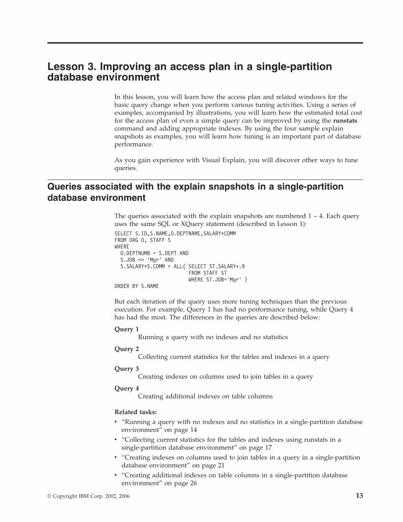
1. Do current statistics exist for each table in the query?
To check if current statistics exist for each table in the query, double-click each
table node in the access plan graph. In the Table Statistics window that opens,
the STATS_TIME row under the Explained column contains the words
″Statistics not updated″ if no statistics had been collected at the time when the
snapshot was created.
If current statistics do not exist, the optimizer uses default statistics, which
might differ from the actual statistics. Default statistics are identified by the
word ″default″ under the Explained column in the Table Statistics window.
According to the information in the Table Statistics window for the ORG table,
the optimizer used default statistics (as indicated next to the explained values).
Default statistics were used because actual statistics were not available when
the snapshot was created (as indicated in the STATS_TIME row).
Lesson 3. Improving an access plan in a single-partition database environment 15
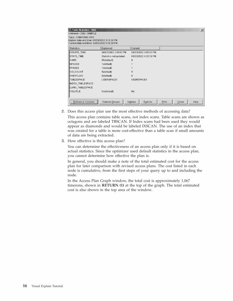
2. Does this access plan use the most effective methods of accessing data?
This access plan contains table scans, not index scans. Table scans are shown as
octagons and are labeled TBSCAN. If Index scans had been used they would
appear as diamonds and would be labeled IXSCAN. The use of an index that
was created for a table is more cost-effective than a table scan if small amounts
of data are being extracted.
3. How effective is this access plan?
You can determine the effectiveness of an access plan only if it is based on
actual statistics. Since the optimizer used default statistics in the access plan,
you cannot determine how effective the plan is.
In general, you should make a note of the total estimated cost for the access
plan for later comparison with revised access plans. The cost listed in each
node is cumulative, from the first steps of your query up to and including the
node.
In the Access Plan Graph window, the total cost is approximately 1,067
timerons, shown in RETURN (1) at the top of the graph. The total estimated
cost is also shown in the top area of the window.
16 Visual Explain Tutorial

4. What’s next?
Query 2 looks at an access plan for the basic query after runstats has been run.
Using the runstats command provides the optimizer with current statistics on
all tables accessed by the query.
Related concepts:
v “Access plan graph node” on page 49
v “Cost” on page 50
Related reference:
v “TBSCAN operator” on page 69
v “IXSCAN operator” on page 65
Collecting current statistics for the tables and indexes using runstats
in a single-partition database environment
This example builds on the access plan described in Query 1 by collecting current
statistics with the runstats command.
It is highly recommended that you use the runstats command to collect current
statistics on tables and indexes, especially if significant update activity has
occurred or new indexes have been created since the last time the runstats
command was executed. This provides the optimizer with the most accurate
Lesson 3. Improving an access plan in a single-partition database environment 17
information with which to determine the best access plan. If current statistics are
not available, the optimizer can choose an inefficient access plan based on
inaccurate default statistics.
Be sure to use runstats after making your table updates; otherwise, the table might
appear to the optimizer to be empty. This problem is evident if cardinality on the
Operator Details window equals zero. In this case, complete your table updates,
rerun the runstats command, and recreate the explain snapshots for affected tables.
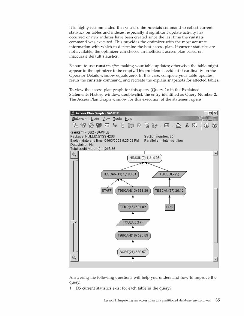
To view the access plan graph for this query (Query 2): in the Explained
Statements History window, double-click on the entry identified as Query Number
2. The Access Plan Graph window for this execution of the statement opens.
Answering the following questions will help you understand how to improve the
query.
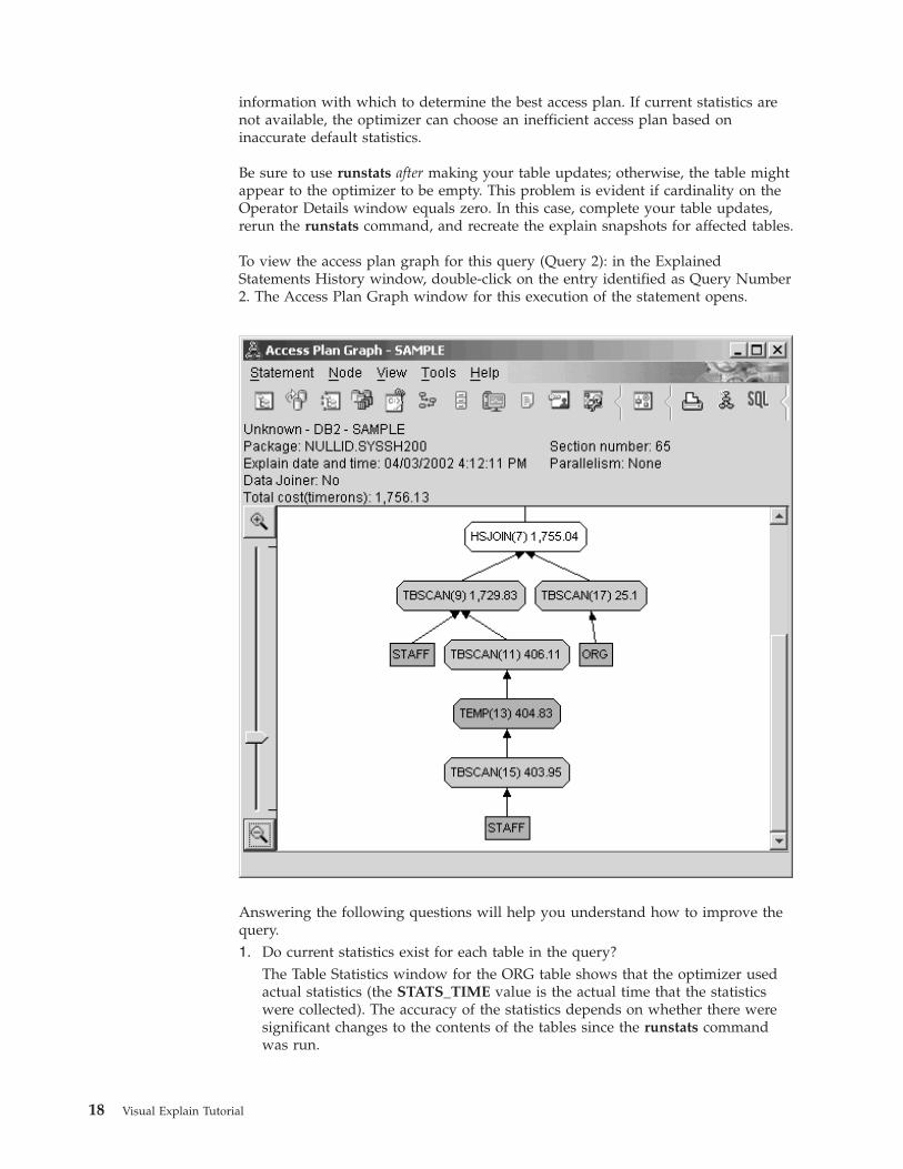
1. Do current statistics exist for each table in the query?
The Table Statistics window for the ORG table shows that the optimizer used
actual statistics (the STATS_TIME value is the actual time that the statistics
were collected). The accuracy of the statistics depends on whether there were
significant changes to the contents of the tables since the runstats command
was run.
18 Visual Explain Tutorial
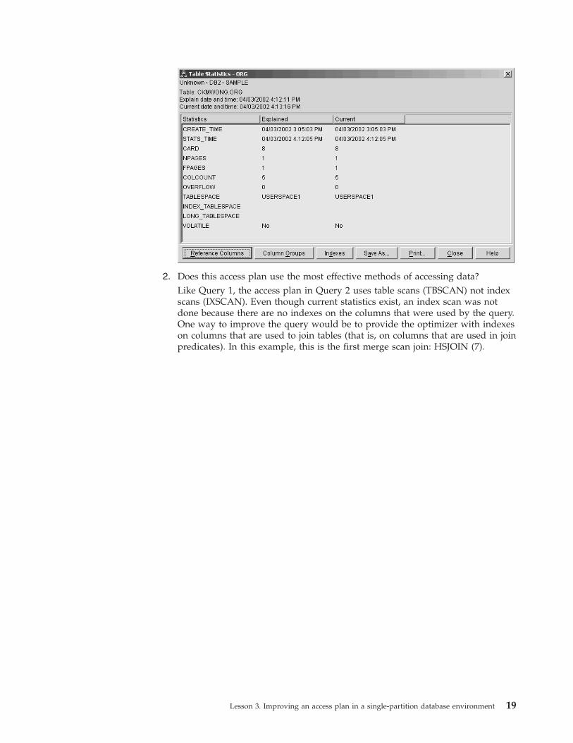
2. Does this access plan use the most effective methods of accessing data?
Like Query 1, the access plan in Query 2 uses table scans (TBSCAN) not index
scans (IXSCAN). Even though current statistics exist, an index scan was not
done because there are no indexes on the columns that were used by the query.
One way to improve the query would be to provide the optimizer with indexes
on columns that are used to join tables (that is, on columns that are used in join
predicates). In this example, this is the first merge scan join: HSJOIN (7).
Lesson 3. Improving an access plan in a single-partition database environment 19
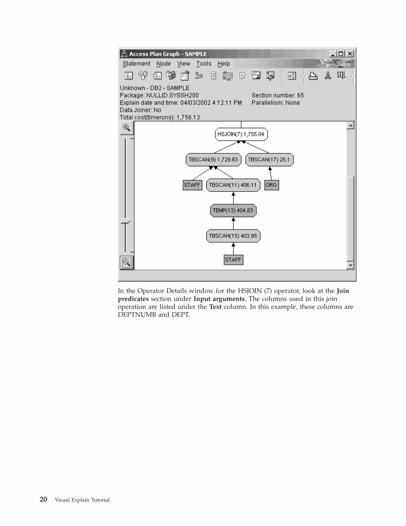
In the Operator Details window for the HSJOIN (7) operator, look at the Join
predicates section under Input arguments. The columns used in this join
operation are listed under the Text column. In this example, these columns are
DEPTNUMB and DEPT.
20 Visual Explain Tutorial

3. How effective is this access plan?
Access plans based on up-to-date statistics always produce a realistic estimated
cost (measured in timerons). Because the estimated cost in Query 1 was based
on default statistics, the cost of the two access plan graphs cannot be compared
in order to determine which one is more effective. Whether the cost is higher or
lower is not relevant. You must compare the cost of access plans that are based
on actual statistics to get a valid measurement of effectiveness.
4. What’s next?
Query 3 looks at the effects of adding indexes on the DEPTNUMB and DEPT
columns. Adding indexes on the columns that are used in join predicates can
improve performance.
Related concepts:
v “Predicate” on page 55
Related reference:
v “TBSCAN operator” on page 69
v “IXSCAN operator” on page 65
Creating indexes on columns used to join tables in a query in a
single-partition database environment
This example builds on the access plan described in Query 2 by creating indexes
on the DEPT column on the STAFF table and on the DEPTNUMB column on the
ORG table. Recommended indexes can be created using the Design Advisor.
To view the access plan graph for this query (Query 3): in the Explained
Statements History window, double-click the entry identified as Query Number 3.
The Access Plan Graph window for this execution of the statement opens.
Lesson 3. Improving an access plan in a single-partition database environment 21

Note: Even though an index was created for DEPTNUM, the optimizer did not use
it.
Answering the following questions will help you understand how to improve the
query.
1. What has changed in the access plan with indexes?
A nested loop join, NLJOIN (7), has replaced the merge scan join HSJOIN (7)
that was used in Query 2. Using a nested loop join resulted in a lower
estimated cost than a merge scan join because this type of join does not require
any sort or temporary tables.
A new diamond-shaped node, I_DEPT, has been added just above the STAFF
table. This node represents the index that was created on DEPT, and it shows
that the optimizer used an index scan instead of a table scan to determine
which rows to retrieve.
22 Visual Explain Tutorial
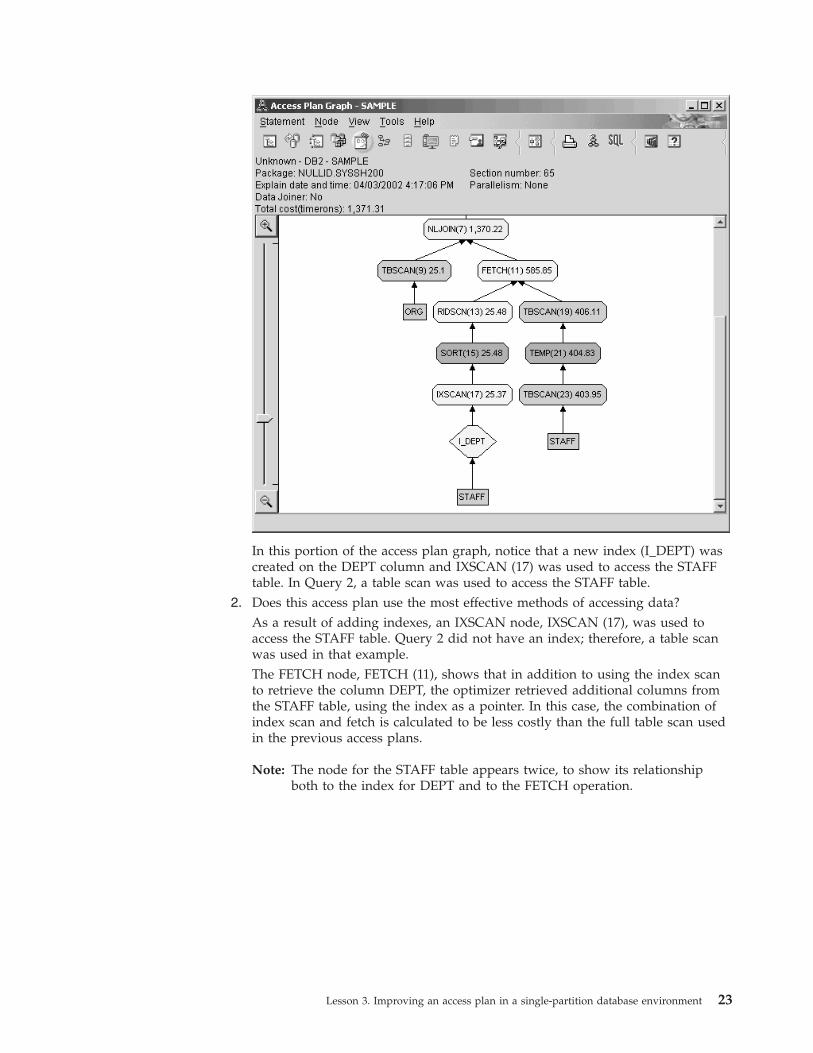
In this portion of the access plan graph, notice that a new index (I_DEPT) was
created on the DEPT column and IXSCAN (17) was used to access the STAFF
table. In Query 2, a table scan was used to access the STAFF table.
2. Does this access plan use the most effective methods of accessing data?
As a result of adding indexes, an IXSCAN node, IXSCAN (17), was used to
access the STAFF table. Query 2 did not have an index; therefore, a table scan
was used in that example.
The FETCH node, FETCH (11), shows that in addition to using the index scan
to retrieve the column DEPT, the optimizer retrieved additional columns from
the STAFF table, using the index as a pointer. In this case, the combination of
index scan and fetch is calculated to be less costly than the full table scan used
in the previous access plans.
Note: The node for the STAFF table appears twice, to show its relationship
both to the index for DEPT and to the FETCH operation.
Lesson 3. Improving an access plan in a single-partition database environment 23

The access plan for this query shows the effect of creating indexes on columns
involved in join predicates. Indexes can also speed up the application of local
predicates. Let’s look at the local predicates for each table in this query to see
how adding indexes to columns referenced in local predicates might affect the
access plan.
In the Operator Details window for the FETCH (11) operator, look at the
columns under Cumulative Properties. The column used in the predicate for
this fetch operation is JOB, as shown in the Predicates section.
Note: The selectivity of this predicate is .69. This means that with this
predicate, 69% of the rows will be selected for further processing.
24 Visual Explain Tutorial
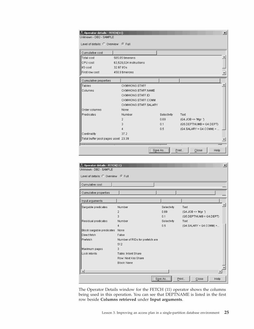
The Operator Details window for the FETCH (11) operator shows the columns
being used in this operation. You can see that DEPTNAME is listed in the first
row beside Columns retrieved under Input arguments.
Lesson 3. Improving an access plan in a single-partition database environment 25

3. How effective is this access plan?
This access plan is more cost effective than the one from the previous example.
The cumulative cost has been reduced from approximately 1,755 timerons in
Query 2 to approximately 959 timerons in Query 3.
However, the access plan for Query 3 shows an index scan IXSCAN (17) and a
FETCH (11) for the STAFF table. While an index scan combined with a fetch
operation is less costly than a full table scan, it means that for each row
retrieved, the table is accessed once and the index is accessed once. Let’s try to
reduce this double access on the STAFF table.
4. What’s next?
Query 4 reduces the fetch and index scan to a single index scan without a
fetch. Creating additional indexes might reduce the estimated cost for the
access plan.
Related concepts:
v “Access plan graph node” on page 49
v “Predicate” on page 55
Related reference:
v “NLJOIN operator” on page 66
v “IXSCAN operator” on page 65
v “FETCH operator” on page 62
Creating additional indexes on table columns in a single-partition
database environment
This example builds on the access plan described in Query 3 by creating an index
on the JOB column in the STAFF table, and adding DEPTNAME to the existing
index in the ORG table.(Adding a separate index could cause an additional access.)
To view the access plan graph for this query (Query 4): in the Explained
Statements History window, double-click the entry identified as Query Number 4.
The Access Plan Graph window for this execution of the statement opens.
26 Visual Explain Tutorial

Lesson 3. Improving an access plan in a single-partition database environment 27

Answering the following questions will help you understand how to improve the
query.
1. What changed in this access plan as a result of creating additional indexes?
The optimizer has taken advantage of the index created on the JOB column in
the STAFF table (represented by a diamond labeled I_JOB) to further refine this
access plan.
28 Visual Explain Tutorial
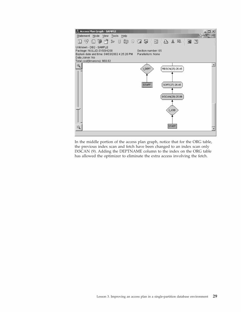
In the middle portion of the access plan graph, notice that for the ORG table,
the previous index scan and fetch have been changed to an index scan only
IXSCAN (9). Adding the DEPTNAME column to the index on the ORG table
has allowed the optimizer to eliminate the extra access involving the fetch.
Lesson 3. Improving an access plan in a single-partition database environment 29

2. How effective is this access plan?
This access plan is more cost effective than the one from the previous example.
The cumulative cost has been reduced from approximately 1,370 timerons in
Query 3 to approximately 959 timerons in Query 4.
30 Visual Explain Tutorial

Lesson 4. Improving an access plan in a partitioned database
environment
In this lesson, you will learn how the access plan and related windows for the
basic query change when you perform various tuning activities. Using a series of
examples, accompanied by illustrations, you will learn how the estimated total cost
for the access plan of even a simple query can be improved by using the runstats
command and adding appropriate indexes. By using the four sample explain
snapshots as examples, you will learn how tuning is an important part of database
performance.
As you gain experience with Visual Explain, you will discover other ways to tune
queries.
Queries associated with the explain snapshots in a partitioned
database environment
The queries associated with the explain snapshots are numbered 1 – 4. Each query
uses the same SQL or XQuery statement (described in Lesson 1):
SELECT S.ID,S.NAME,O.DEPTNAME,SALARY+COMM
FROM ORG O, STAFF S
WHERE
O.DEPTNUMB = S.DEPT AND
S.JOB <> ’Mgr’ AND
S.SALARY+S.COMM > ALL( SELECT ST.SALARY*.9
FROM STAFF ST
WHERE ST.JOB=’Mgr’ )
ORDER BY S.NAME
But each iteration of the query uses more tuning techniques than the previous
execution. For example, Query 1 has had no performance tuning, while Query 4
has had the most. The differences in the queries are described below:
Query 1
Running a query with no indexes and no statistics
Query 2
Collecting current statistics for the tables and indexes in a query
Query 3
Creating indexes on columns used to join tables in a query
Query 4
Creating additional indexes on table columns
These examples were produced on a DB2 Enterprise Extended Edition NT 2000
machine with 7 physical nodes using inter-partition parallelism.
Related tasks:
v “Running a query with no indexes and no statistics in a partitioned database
environment” on page 32
v “Collecting current statistics for the tables and indexes using runstats in a
partitioned database environment” on page 34
© Copyright IBM Corp. 2002, 2006 31

v “Creating indexes on columns used to join tables in a query in a partitioned
database environment” on page 38
v “Creating additional indexes on table columns in a partitioned database
environment” on page 42
Running a query with no indexes and no statistics in a partitioned
database environment
In this example the access plan was created for the SQL query with no indexes and
no statistics.
To view the access plan graph for this query (Query 1):
1. In the Control Center, expand the object tree until you find the SAMPLE
database.
2. Right-click the database and select Show explained statements history from
the pop-up menu. The Explained Statements History window opens.
3. Double-click the entry identified as Query Number 1 (you might need to scroll
to the right to find the Query Number column). The Access Plan Graph
window for the statement opens.
Answering the following questions will help you understand how to improve the
query.
1. Do current statistics exist for each table in the query?
32 Visual Explain Tutorial

To check if current statistics exist for each table in the query, double-click on
each table node in the access plan graph. In the corresponding Table Statistics
window that opens, the STATS_TIME row under the Explained column
contains the words ″Statistics not updated″ indicating that no statistics had
been collected at the time when the snapshot was created.
If current statistics do not exist, the optimizer uses default statistics, which
might differ from the actual statistics. Default statistics are identified by the
word ″default″ under the Explained column in the Table Statistics window.
According to the information in the Table Statistics window for the ORG table,
the optimizer used default statistics (as indicated next to the explained values).
Default statistics were used because actual statistics were not available when
the snapshot was created (as indicated in the STATS_TIME row).
2. Does this access plan use the most effective methods of accessing data?
This access plan contains table scans, not index scans. Table scans are shown as
octagons and are labeled TBSCAN. If Index scans had been used they would
appear as diamonds and be labeled IXSCAN. The use of an index that was
created for a table is more cost-effective than a table scan if small amounts of
data are being extracted.
3. How effective is this access plan?
You can determine the effectiveness of an access plan only if it is based on
actual statistics. Since the optimizer used default statistics in the access plan,
you cannot determine how effective the plan is.
In general, you should make a note of the total estimated cost for the access
plan for later comparison with revised access plans. The cost listed in each
node is cumulative, from the first steps of your query up to and including the
node.
Note: For partitioned databases, this is the cumulative cost for the node that
uses the most resources.
Lesson 4. Improving an access plan in a partitioned database environment 33

In the Access Plan Graph window, the total cost is approximately 1,234
timerons, shown in RETURN (1) at the top of the graph. The total estimated
cost is also shown in the top area of the window.
4. What’s next?
Query 2 looks at an access plan for the basic query after runstats has been run.
Using the runstats command provides the optimizer with current statistics on
all tables accessed by the query.
Related concepts:
v “Access plan graph node” on page 49
v “Cost” on page 50
Related reference:
v “TBSCAN operator” on page 69
v “IXSCAN operator” on page 65
Collecting current statistics for the tables and indexes using runstats
in a partitioned database environment
This example builds on the access plan described in Query 1 by collecting current
statistics with the runstats command.
34 Visual Explain Tutorial
It is highly recommended that you use the runstats command to collect current
statistics on tables and indexes, especially if significant update activity has
occurred or new indexes have been created since the last time the runstats
command was executed. This provides the optimizer with the most accurate
information with which to determine the best access plan. If current statistics are
not available, the optimizer can choose an inefficient access plan based on
inaccurate default statistics.
Be sure to use runstats after making your table updates; otherwise, the table might
appear to the optimizer to be empty. This problem is evident if cardinality on the
Operator Details window equals zero. In this case, complete your table updates,
rerun the runstats command, and recreate the explain snapshots for affected tables.
To view the access plan graph for this query (Query 2): in the Explained
Statements History window, double-click the entry identified as Query Number 2.
The Access Plan Graph window for this execution of the statement opens.
Answering the following questions will help you understand how to improve the
query.
1. Do current statistics exist for each table in the query?
Lesson 4. Improving an access plan in a partitioned database environment 35

The Table Statistics window for the ORG table shows that the optimizer used
actual statistics (the STATS_TIME value is the actual time that the statistics
were collected). The accuracy of the statistics depends on whether there were
significant changes to the contents of the tables since the runstats command
was run.
2. Does this access plan use the most effective methods of accessing data?
Like Query 1, the access plan in Query 2 uses table scans (TBSCAN) not index
scans (IXSCAN). Even though current statistics exist, an index scan was not
done because there are no indexes on the columns that were used by the query.
One way to improve the query would be to provide the optimizer with indexes
on columns that are used to join tables (that is, on columns that are used in join
predicates). In this example, this is the first merge scan join: HSJOIN (9).
36 Visual Explain Tutorial

In the Operator Details window for the HSJOIN (9) operator, look at the Join
predicates section under Input arguments. The columns used in this join
operation are listed under the Text column. In this example, these columns are
DEPTNUMB and DEPT.
Lesson 4. Improving an access plan in a partitioned database environment 37
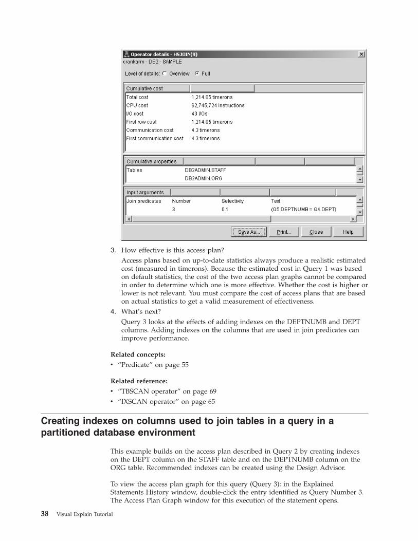
3. How effective is this access plan?
Access plans based on up-to-date statistics always produce a realistic estimated
cost (measured in timerons). Because the estimated cost in Query 1 was based
on default statistics, the cost of the two access plan graphs cannot be compared
in order to determine which one is more effective. Whether the cost is higher or
lower is not relevant. You must compare the cost of access plans that are based
on actual statistics to get a valid measurement of effectiveness.
4. What’s next?
Query 3 looks at the effects of adding indexes on the DEPTNUMB and DEPT
columns. Adding indexes on the columns that are used in join predicates can
improve performance.
Related concepts:
v “Predicate” on page 55
Related reference:
v “TBSCAN operator” on page 69
v “IXSCAN operator” on page 65
Creating indexes on columns used to join tables in a query in a
partitioned database environment
This example builds on the access plan described in Query 2 by creating indexes
on the DEPT column on the STAFF table and on the DEPTNUMB column on the
ORG table. Recommended indexes can be created using the Design Advisor.
To view the access plan graph for this query (Query 3): in the Explained
Statements History window, double-click the entry identified as Query Number 3.
The Access Plan Graph window for this execution of the statement opens.
38 Visual Explain Tutorial

Note: Even though an index was created for DEPTNUM, the optimizer did not use
it.
Answering the following questions will help you understand how to improve the
query.
1. What has changed in the access plan with indexes?
A new diamond-shaped node, I_DEPT, has been added just above the STAFF
table. This node represents the index that was created on DEPT, and it shows
that the optimizer used an index scan instead of a table scan to determine
which rows to retrieve.
Lesson 4. Improving an access plan in a partitioned database environment 39

2. Does this access plan use the most effective methods of accessing data?
The access plan for this query shows the effect of creating indexes on the
DEPTNUMB column of the ORG table, resulting in FETCH (15) and IXSCAN
(21) and on the DEPT column of the STAFF table. Query 2 did not have this
index; therefore, a table scan was used in that example.
40 Visual Explain Tutorial

The Operator Details window for the FETCH(15) operator shows the columns
being used in this operation.
Lesson 4. Improving an access plan in a partitioned database environment 41
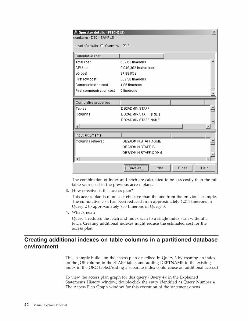
The combination of index and fetch are calculated to be less costly than the full
table scan used in the previous access plans.
3. How effective is this access plan?
This access plan is more cost effective than the one from the previous example.
The cumulative cost has been reduced from approximately 1,214 timerons in
Query 2 to approximately 755 timerons in Query 3.
4. What’s next?
Query 4 reduces the fetch and index scan to a single index scan without a
fetch. Creating additional indexes might reduce the estimated cost for the
access plan.
Creating additional indexes on table columns in a partitioned database
environment
This example builds on the access plan described in Query 3 by creating an index
on the JOB column in the STAFF table, and adding DEPTNAME to the existing
index in the ORG table.(Adding a separate index could cause an additional access.)
To view the access plan graph for this query (Query 4): in the Explained
Statements History window, double-click the entry identified as Query Number 4.
The Access Plan Graph window for this execution of the statement opens.
42 Visual Explain Tutorial

Answering the following questions will help you understand how to improve the
query.
1. What changed in this access plan as a result of creating additional indexes?
In the middle portion of the access plan graph, notice that for the ORG table,
the previous table scan has been changed to an index scan, IXSCAN (7).
Adding the DEPTNAME column to the index on the ORG table has allowed
the optimizer to refine the access involving the table scan.
Lesson 4. Improving an access plan in a partitioned database environment 43
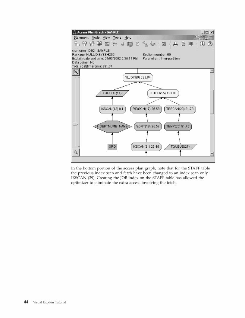
In the bottom portion of the access plan graph, note that for the STAFF table
the previous index scan and fetch have been changed to an index scan only
IXSCAN (39). Creating the JOB index on the STAFF table has allowed the
optimizer to eliminate the extra access involving the fetch.
44 Visual Explain Tutorial
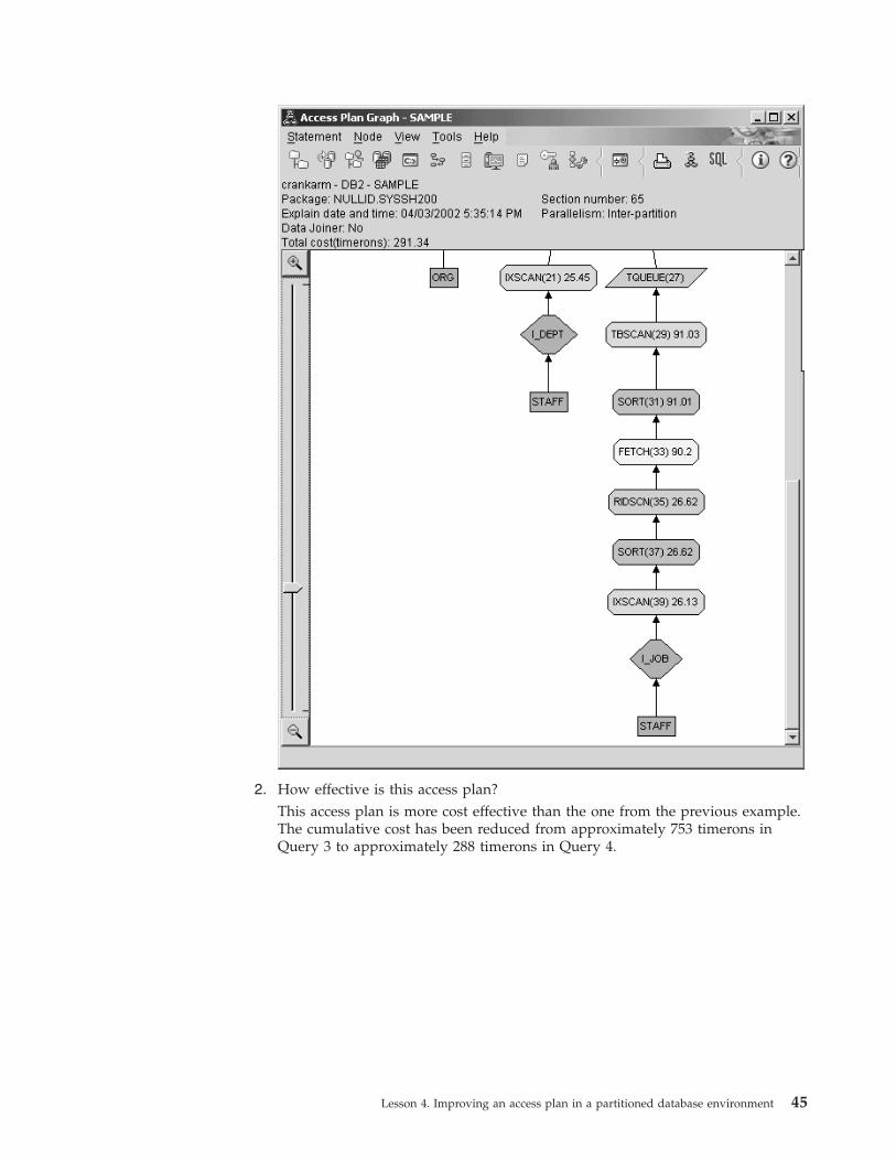
2. How effective is this access plan?
This access plan is more cost effective than the one from the previous example.
The cumulative cost has been reduced from approximately 753 timerons in
Query 3 to approximately 288 timerons in Query 4.
Lesson 4. Improving an access plan in a partitioned database environment 45

46 Visual Explain Tutorial

Appendix A. Visual Explain concepts
v Access plan
v Access plan graph
v Access plan graph node
v Clustering
v Container
v Cost
v Cursor blocking
v Database-managed table space
v Dynamic SQL or XQuery
v Explain snapshot
v Explainable statement
v Explained statement
v Operand
v Operator
v Optimizer
v Package
v Predicate
v Query optimization class
v Selectivity of predicates
v Star join
v Static SQL or XQuery
v System-managed table space
v Table spaces
v Timerons
v Visual Explain
Access plan
Certain data is necessary to resolve an explainable SQL or XQuery statement. An
access plan specifies an order of operations for accessing this data. An access plan
lets you view statistics for selected tables, indexes, or columns; properties for
operators; global information such as table space and function statistics; and
configuration parameters relevant to optimization. With Visual Explain, you can
view the access plan for an SQL or XQuery statement in graphical form.
The optimizer produces an access plan whenever you compile an explainable SQL
or XQuery statement. This happens at prep/bind time for static statements, and at
run time for dynamic statements.
It is important to understand that an access plan is an estimate based on the
information that is available. The optimizer bases its estimations on information
such as the following:
v Statistics in system catalog tables (if statistics are not current, update them using
the RUNSTATS command.)
v Configuration parameters
© Copyright IBM Corp. 2002, 2006 47

v Bind options
v The query optimization class
Cost information associated with an access plan is the optimizer’s best estimate of
the resource usage for a query. The actual elapsed time for a query might vary
depending on factors outside the scope of DB2 (for example, the number of other
applications running at the same time). Actual elapsed time can be measured while
running the query, by using performance monitoring.
Related concepts:
v “Access plan graph” on page 48
v “Visual Explain overview” in Administration Guide: Implementation
Related tasks:
v “Dynamically explaining an SQL or an XQuery statement” in Administration
Guide: Implementation
v “Viewing a graphical representation of an access plan” in Administration Guide:
Implementation
v “Viewing explainable statements for a package” in Administration Guide:
Implementation
v “Viewing the history of previously explained query statements” in Administration
Guide: Implementation
Access plan graph
Visual Explain uses information from a number of sources in order to produce an
access plan graph, as shown in the illustration below. Based on various inputs, the
optimizer chooses an access plan, and Visual Explain displays it in an access plan
graph. The nodes in the graph represent tables and indexes and each operation on
them. The links between the nodes represent the flow of data.
Related concepts:
v “Access plan” on page 47
48 Visual Explain Tutorial

v “Visual Explain overview” in Administration Guide: Implementation
Related tasks:
v “Viewing the history of previously explained query statements” in Administration
Guide: Implementation
v “Dynamically explaining an SQL or an XQuery statement” in Administration
Guide: Implementation
v “Viewing a graphical representation of an access plan” in Administration Guide:
Implementation
v “Viewing explainable statements for a package” in Administration Guide:
Implementation
Access plan graph node
The access plan graph consists of a tree displaying nodes. These nodes represent:
v Tables, shown as rectangles
v Indexes, shown as diamonds
v Operators, shown as octagons (8 sides). TQUEUE operators, shown as
parallelograms
v Table functions, shown as hexagons(6 sides).
Related concepts:
v “Access plan” on page 47
v “Access plan graph” on page 48
Clustering
Over time, updates may cause rows on data pages to change location lowering the
degree of clustering that exists between an index and the data pages. Reorganizing
a table with respect to a chosen index reclusters the data. A clustered index is most
useful for columns that have range predicates because it allows better sequential
access of data in the base table. This results in fewer page fetches, since like values
are on the same data page.
In general, only one of the indexes in a table can have a high degree of clustering.
To check the degree of clustering for an index, double-click on its node to display
the Index Statistics window. The cluster ratio or cluster factor values are shown in
this window. If the value is low, consider reorganizing the table’s data.
Related reference:
v “Guidelines for creating indexes” on page 79
Container
A container is a physical storage location of the data. It is associated with a table
space, and can be a file or a directory or a device.
Related concepts:
v “Table spaces” on page 58
Appendix A. Visual Explain concepts 49

Cost
Cost, in the context of Visual Explain, is the estimated total resource usage
necessary to execute the access plan for a statement (or the elements of a
statement). Cost is derived from a combination of CPU cost (in number of
instructions) and I/O (in numbers of seeks and page transfers).
The unit of cost is the timeron. A timeron does not directly equate to any actual
elapsed time, but gives a rough relative estimate of the resources (cost) required by
the database manager to execute two plans for the same query.
The cost shown in each operator node of an access plan graph is the cumulative
cost, from the start of access plan execution up to and including the execution of
that particular operator. It does not reflect factors such as the workload on the
system or the cost of returning rows of data to the user.
Related concepts:
v “Timerons” on page 59
Cursor blocking
Cursor blocking is a technique that reduces overhead by having the database
manager retrieve a block of rows in a single operation. These rows are stored in a
cache while they are processed. The cache is allocated when an application issues
an OPEN CURSOR request, and is de-allocated when the cursor is closed. When
all the rows have been processed, another block of rows is retrieved.
Use the BLOCKING option on the PREP or BIND commands along with the
following parameters to specify the type of cursor blocking:
UNAMBIG
Only unambiguous cursors are blocked (the default).
ALL Both ambiguous and unambiguous cursors are blocked.
NO Cursors are not blocked.
Related tasks:
v “Specifying row blocking to reduce overhead” in Performance Guide
Related reference:
v “BIND command” in Command Reference
v “PRECOMPILE command” in Command Reference
Database-managed table space
There are two types of table spaces that can exist in a database: Database-managed
space (DMS), and system-managed space (SMS).
DMS table spaces are managed by the database manager. and are designed and
tuned to meet its requirements.
The DMS table space definition includes a list of files (or devices) into which the
database data is stored in its DMS table space format.
50 Visual Explain Tutorial

You can add pre-allocated files (or devices) to an existing DMS table space in order
to increase its storage capacity. The database manager automatically rebalances
existing data in all the containers belonging to that table space.
DMS and SMS table spaces can coexist in the same database.
Related concepts:
v “System-managed table space” on page 58
Dynamic SQL or XQuery
Dynamic SQL or XQuery statements are SQL or XQuery statements that are prepared
and executed within an application program while the program is running. In
dynamic SQL or XQuery, either:
v You issue the SQL or XQuery statement interactively, using CLI or CLP
v The SQL or XQuery source is contained in host language variables that are
embedded in an application program.
When DB2 runs a dynamic SQL or XQuery statement, it creates an access plan that
is based on current catalog statistics and configuration parameters. This access plan
might change from one execution of the statements application program to the
next.
The alternative to dynamic SQL or XQuery is static SQL or XQuery.
Related concepts:
v “Static SQL or XQuery” on page 58
Explain snapshot
With Visual Explain, you can examine the contents of an explain snapshot.
An explain snapshot is compressed information that is collected when an SQL
statement is explained. It is stored as a binary large object (BLOB) in the
EXPLAIN_STATEMENT table, and contains the following information:
v The internal representation of the access plan, including its operators and the
tables and indexes accessed
v The decision criteria used by the optimizer, including statistics for database
objects and the cumulative cost for each operation.
An explain snapshot is required if you want to display the graphical representation
of an SQL statement’s access plan. To ensure that an explain snapshot is created:
1. Explain tables must exist in the database manager to store the explain
snapshots. For information on how to create these tables, see Creating explain
tables in the online help.
2. For a package containing static SQL or XQuery statements, set the EXPLSNAP
option to ALL or YES when you bind or prep the package. You will get an
explain snapshot for each explainable SQL statement in the package. For more
information on the BIND and PREP commands, see the Command Reference.
3. For dynamic SQL statements, set the EXPLSNAP option to ALL when you bind
the application that issues them, or set the CURRENT EXPLAIN SNAPSHOT
Appendix A. Visual Explain concepts 51

special register to YES or EXPLAIN before you issue them interactively. For
more information, see the section on current explain snapshots in the SQL
Reference.
Related tasks:
v “Using explain snapshots” on page 3
Related reference:
v “BIND command” in Command Reference
v “PRECOMPILE command” in Command Reference
Explainable statement
An explainable statement is an SQL or XQuery statement for which an explain
operation can be performed.
Explainable SQL or XQuery statements are:
v SELECT
v INSERT
v UPDATE
v DELETE
v VALUES
Related concepts:
v “Explained statement” on page 52
Explained statement
An explained statement is an SQL or XQuery statement for which an explain
operation has been performed. Explained statements are shown in the Explained
Statements History window.
Related concepts:
v “Explainable statement” on page 52
Operand
An operand is an entity on which an operation is performed. For example, a table
or an index is an operand of various operators such as TBSCAN and IXSCAN.
Related concepts:
v “Operator” on page 52
Operator
An operator is either an action that must be performed on data, or the output from
a table or an index, when the access plan for an SQL or XQuery statement is
executed.
The following operators can appear in the access plan graph:
52 Visual Explain Tutorial
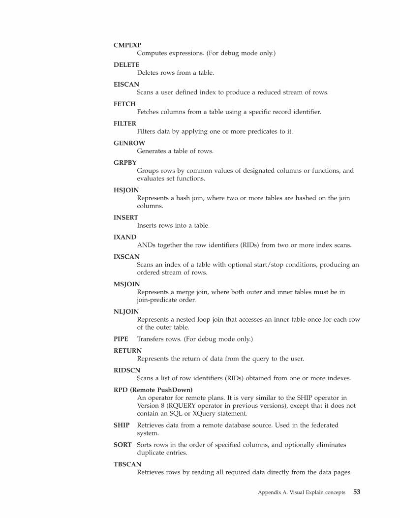
CMPEXP
Computes expressions. (For debug mode only.)
DELETE
Deletes rows from a table.
EISCAN
Scans a user defined index to produce a reduced stream of rows.
FETCH
Fetches columns from a table using a specific record identifier.
FILTER
Filters data by applying one or more predicates to it.
GENROW
Generates a table of rows.
GRPBY
Groups rows by common values of designated columns or functions, and
evaluates set functions.
HSJOIN
Represents a hash join, where two or more tables are hashed on the join
columns.
INSERT
Inserts rows into a table.
IXAND
ANDs together the row identifiers (RIDs) from two or more index scans.
IXSCAN
Scans an index of a table with optional start/stop conditions, producing an
ordered stream of rows.
MSJOIN
Represents a merge join, where both outer and inner tables must be in
join-predicate order.
NLJOIN
Represents a nested loop join that accesses an inner table once for each row
of the outer table.
PIPE Transfers rows. (For debug mode only.)
RETURN
Represents the return of data from the query to the user.
RIDSCN
Scans a list of row identifiers (RIDs) obtained from one or more indexes.
RPD (Remote PushDown)
An operator for remote plans. It is very similar to the SHIP operator in
Version 8 (RQUERY operator in previous versions), except that it does not
contain an SQL or XQuery statement.
SHIP Retrieves data from a remote database source. Used in the federated
system.
SORT Sorts rows in the order of specified columns, and optionally eliminates
duplicate entries.
TBSCAN
Retrieves rows by reading all required data directly from the data pages.
Appendix A. Visual Explain concepts 53

TEMP Stores data in a temporary table to be read back out (possibly multiple
times).
TQUEUE
Transfers table data between database agents.
UNION
Concatenates streams of rows from multiple tables.
UNIQUE
Eliminates rows with duplicate values, for specified columns.
UPDATE
Updates rows in a table.
XISCAN
Scans an index of an XML table.
XSCAN
Navigates an XML document node subtrees.
XANDOR
Allows ANDed and ORed predicates to be applied to multiple XML
indexes.
Related concepts:
v “Operand” on page 52
Optimizer
The optimizer is the component of the SQL compiler that chooses an access plan for
a data manipulation language (DML) SQL statement. It does this by modeling the
execution cost of many alternative access plans, and choosing the one with the
minimal estimated cost.
Related concepts:
v “Query optimization class” on page 55
Package
A package is an object stored in the database that includes the information needed
to process the SQL statements associated with one source file of an application
program. It is generated by either:
v Precompiling a source file with the PREP command
v Binding a bind file that was generated by the precompiler with the BIND
command.
Related reference:
v “BIND command” in Command Reference
v “PRECOMPILE command” in Command Reference
54 Visual Explain Tutorial
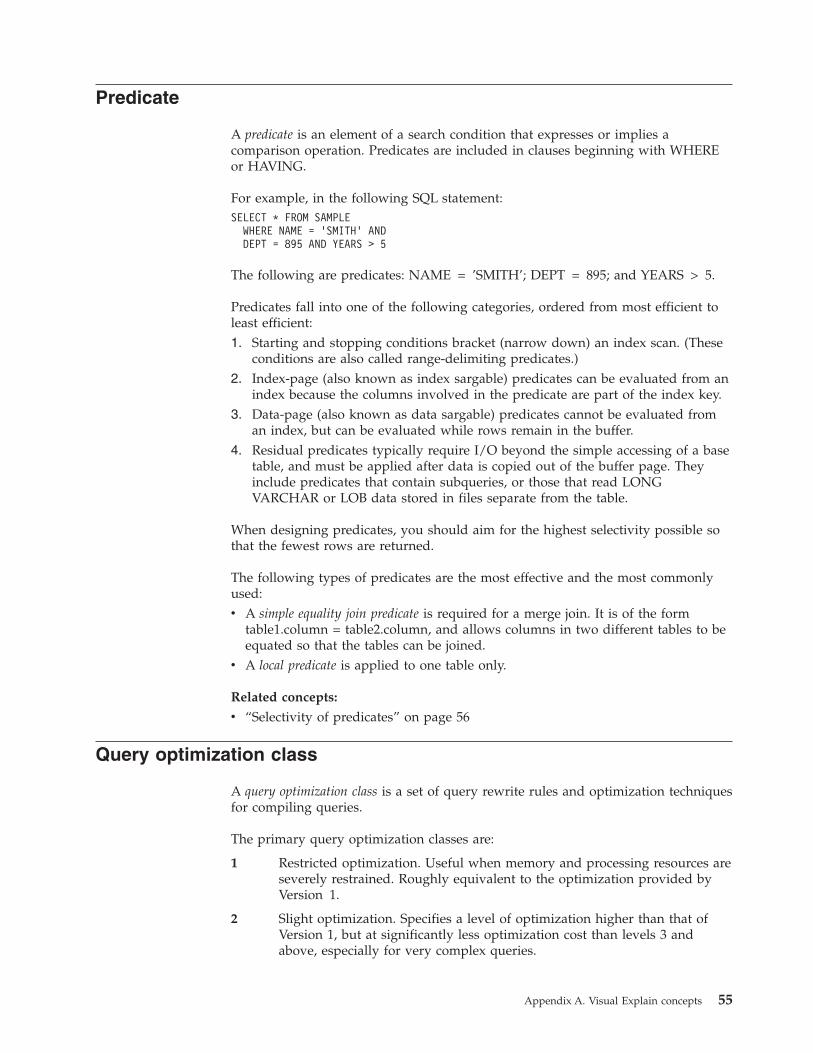
Predicate
A predicate is an element of a search condition that expresses or implies a
comparison operation. Predicates are included in clauses beginning with WHERE
or HAVING.
For example, in the following SQL statement:
SELECT * FROM SAMPLE
WHERE NAME = ’SMITH’ AND
DEPT = 895 AND YEARS > 5
The following are predicates: NAME = ’SMITH’; DEPT = 895; and YEARS > 5.
Predicates fall into one of the following categories, ordered from most efficient to
least efficient:
1. Starting and stopping conditions bracket (narrow down) an index scan. (These
conditions are also called range-delimiting predicates.)
2. Index-page (also known as index sargable) predicates can be evaluated from an
index because the columns involved in the predicate are part of the index key.
3. Data-page (also known as data sargable) predicates cannot be evaluated from
an index, but can be evaluated while rows remain in the buffer.
4. Residual predicates typically require I/O beyond the simple accessing of a base
table, and must be applied after data is copied out of the buffer page. They
include predicates that contain subqueries, or those that read LONG
VARCHAR or LOB data stored in files separate from the table.
When designing predicates, you should aim for the highest selectivity possible so
that the fewest rows are returned.
The following types of predicates are the most effective and the most commonly
used:
v A simple equality join predicate is required for a merge join. It is of the form
table1.column = table2.column, and allows columns in two different tables to be
equated so that the tables can be joined.
v A local predicate is applied to one table only.
Related concepts:
v “Selectivity of predicates” on page 56
Query optimization class
A query optimization class is a set of query rewrite rules and optimization techniques
for compiling queries.
The primary query optimization classes are:
1 Restricted optimization. Useful when memory and processing resources are
severely restrained. Roughly equivalent to the optimization provided by
Version 1.
2 Slight optimization. Specifies a level of optimization higher than that of
Version 1, but at significantly less optimization cost than levels 3 and
above, especially for very complex queries.
Appendix A. Visual Explain concepts 55

3 Moderate optimization. Comes closest to matching the query optimization
characteristics of DB2 for MVS™/ESA.
5 Normal optimization. Recommended for a mixed environment using both
simple transactions and complex queries.
7 Normal optimization. The same as query optimization 5 except that it does
not reduce the amount of query optimization for complex dynamic queries.
Other query optimization classes, to be used only under special circumstances, are:
0 Minimal optimization. Use only when little or no optimization is required
(that is, for very simple queries on well-indexed tables).
9 Maximum optimization. Uses substantial memory and processing
resources. Use only if class 5 is insufficient (that is, for very complex and
long-running queries that do not perform well at class 5).
In general, use a higher optimization class for static queries and for queries that
you anticipate will take a long time to execute, and a lower optimization class for
simple queries that are submitted dynamically or that are run only a few times.
To set the query optimization for dynamic SQL or XQuery statements, enter the
following command in the command line processor:
SET CURRENT QUERY OPTIMIZATION = n;
where ’n’ is the desired query optimization class.
To set the query optimization for static SQL or XQuery statements, use the
QUERYOPT option on the BIND or PREP commands.
Related concepts:
v “Optimizer” on page 54
Related reference:
v “BIND command” in Command Reference
v “PRECOMPILE command” in Command Reference
Selectivity of predicates
Selectivity refers to the probability that any row will satisfy a predicate (that is, be
true).
For example, a selectivity of 0.01 (1%) for a predicate operating on a table with
1,000,000 rows means that the predicate returns an estimated 10,000 rows (1% of
1,000,000), and discards an estimated 990,000 rows.
A highly selective predicate (one with a selectivity of 0.10 or less) is desirable. Such
predicates return fewer rows for future operators to work on, thereby requiring
less CPU and I/O to satisfy the query.
Example
Suppose that you have a table of 1,000,000 rows, and that the original query
contains an ’ORDER BY’ clause requiring an additional sorting step. With a
predicate that has a selectivity of 0.01, the sort would have to be done on an
56 Visual Explain Tutorial

estimated 10,000 rows. However, with a less selective predicate of 0.50, the sort
would have to be done on an estimated 500,000 rows, thus requiring more CPU
and I/O time.
Related concepts:
v “Predicate” on page 55
Star join
A set of joins are considered to be a star join when a fact table (large central table)
is joined to two or more dimension tables (smaller tables containing descriptions of
the column values in the fact table).
A Star join is comprised of 3 main parts:
v Semijoins
v Index ANDing of the results of the Semijoins
v Completing the semijoins.
It shows up as two or more joins feeding an IXAND operator.
A Semijoin is a special form of join in which the result of the join is only the Row
Identifier (RID) of the inner table, instead of the joining of the inner and outer
table columns.
Star joins use Semijoins to supply Row Identifiers to an Index ANDing operator.
The Index ANDing operator accumulates the filtering affect of the various joins.
The output from the Index ANDing operator is fed into an Index ORing operator,
which orders the Row Identifiers, and eliminates any duplicate rows that may have
resulted from the joins feeding the Index ANDing operator. The rows from the fact
table are then fetched, using a Fetch operator. Finally, the reduced fact table is
joined to all of the dimension tables, to complete the joins.
Performance suggestions:
v Create indexes on the fact table for each of the dimension table joins.
v Ensure the sort heap threshold is high enough to allow allocating the Index
ANDing operator’s bit filter. For star joins, this could require as much as 12MB,
or 3000 4K pages. For Intra-partition parallelism, the bit filter is allocated from
the same shared memory segment as the shared sort heap, and it is bounded by
the sortheap database configuration parameter and the sheapthres_shr database
configuration parameter.
v Apply filtering predicates against the dimension tables. If statistics are not
current, update them using the runstats command.
Related reference:
v “IXAND operator” on page 65
v “RUNSTATS command” in Command Reference
v “Using RUNSTATS” on page 80
Appendix A. Visual Explain concepts 57

Static SQL or XQuery
A static SQL or XQuery statement is embedded within an application program. All
these embedded statements must be precompiled and bound into a package before
the application can be executed. To execute XQuery expressions in static SQL, use
the XMLQUERY function.
When DB2 compiles these statements, it creates an access plan for each one that is
based on the catalog statistics and configuration parameters at the time that the
statements were precompiled and bound.
These access plans are always used when the application is run; they do not
change until the package is bound again.
The alternative to static SQL or XQuery is dynamic SQL or XQuery.
Related tasks:
v “Executing XQuery expressions in embedded SQL applications” in Developing
Embedded SQL Applications
System-managed table space
There are two types of table spaces that can exist in a database: system-managed
space (SMS) and database-managed space (DMS).
An SMS table space is managed by the operating system, which stores the
database data into a space that is assigned when a table space is created. The table
space definition includes a list of one or more of the directory paths where this
data is stored.
The file system manages the allocation and management of media storage.
SMS and DMS table spaces can coexist in the same database.
Related concepts:
v “Database-managed table space” on page 50
Table spaces
It is easier to manage very large databases if you partition them into separately
managed parts called table spaces.
A table space lets you assign the location of data to particular logical devices or
portions thereof. For example, when creating a table you can specify that its
indexes or its long columns with long or large object (LOB) data be kept away
from the rest of the table data.
A table space can be spread over one or more physical storage devices (containers)
for increased performance. However, it is recommended that all the devices or
containers within a table space have similar performance characteristics.
A table space can be managed in two different ways: as a system-managed space
(SMS) or as a database-managed space (DMS).
58 Visual Explain Tutorial
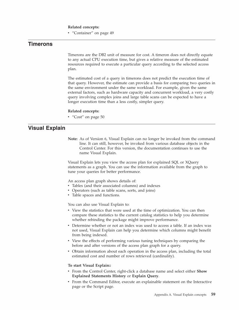
Related concepts:
v “Container” on page 49
Timerons
Timerons are the DB2 unit of measure for cost. A timeron does not directly equate
to any actual CPU execution time, but gives a relative measure of the estimated
resources required to execute a particular query according to the selected access
plan.
The estimated cost of a query in timerons does not predict the execution time of
that query. However, the estimate can provide a basis for comparing two queries in
the same environment under the same workload. For example, given the same
external factors, such as hardware capacity and concurrent workload, a very costly
query involving complex joins and large table scans can be expected to have a
longer execution time than a less costly, simpler query.
Related concepts:
v “Cost” on page 50
Visual Explain
Note: As of Version 6, Visual Explain can no longer be invoked from the command
line. It can still, however, be invoked from various database objects in the
Control Center. For this version, the documentation continues to use the
name Visual Explain.
Visual Explain lets you view the access plan for explained SQL or XQuery
statements as a graph. You can use the information available from the graph to
tune your queries for better performance.
An access plan graph shows details of:
v Tables (and their associated columns) and indexes
v Operators (such as table scans, sorts, and joins)
v Table spaces and functions.
You can also use Visual Explain to:
v View the statistics that were used at the time of optimization. You can then
compare these statistics to the current catalog statistics to help you determine
whether rebinding the package might improve performance.
v Determine whether or not an index was used to access a table. If an index was
not used, Visual Explain can help you determine which columns might benefit
from being indexed.
v View the effects of performing various tuning techniques by comparing the
before and after versions of the access plan graph for a query.
v Obtain information about each operation in the access plan, including the total
estimated cost and number of rows retrieved (cardinality).
To start Visual Explain::
v From the Control Center, right-click a database name and select either Show
Explained Statements History or Explain Query.
v From the Command Editor, execute an explainable statement on the Interactive
page or the Script page.
Appendix A. Visual Explain concepts 59

v From the Query Patroller, click Show Access Plan from either the Managed
Queries Properties notebook or from the Historical Queries Properties notebook.
Related concepts:
v “Visual Explain overview” in Administration Guide: Implementation
60 Visual Explain Tutorial
Appendix B. Alphabetical list of Visual Explain operators
v CMPEXP operator
v DELETE operator
v EISCAN operator
v FETCH operator
v FILTER operator
v GENROW operator
v GRPBY operator
v HSJOIN operator
v INSERT operator
v IXAND operator
v IXSCAN operator
v MSJOIN operator
v NLJOIN operator
v PIPE operator
v RETURN operator
v RIDSCN operator
v RPD operator
v SHIP operator
v SORT operator
v TBSCAN operator
v TEMP operator
v TQUEUE operator
v UNION operator
v UNIQUE operator
v UPDATE operator
v XISCAN operator
v XSCAN operator
v XANDOR operator
CMPEXP operator
Operator name: CMPEXP
Represents: The computation of expressions required for intermediate or final
results.
(This operator is for debug mode only.)
Related concepts:
v “Operator” on page 52
© Copyright IBM Corp. 2002, 2006 61

DELETE operator
Operator name: DELETE
Represents: The deletion of rows from a table.
This operator represents a necessary operation. To improve access plan costs,
concentrate on other operators (such as scans and joins) that define the set of rows
to be deleted.
Performance Suggestion:
v If you are deleting all rows from a table, consider using the DROP TABLE
statement or the LOAD REPLACE command.
Related concepts:
v “Operator” on page 52
EISCAN operator
Operator name: EISCAN
Represents: This operator scans a user defined index to produce a reduced stream
of rows. The scanning uses the multiple start/stop conditions from the user
supplied range producer function.
This operation is performed to narrow down the set of qualifying rows before
accessing the base table (based on predicates).
Performance Suggestion:
v Over time, database updates may cause an index to become fragmented,
resulting in more index pages than necessary. This can be corrected by dropping
and recreating the index, or reorganizing the index.
v If statistics are not current, update them using the runstats command.
Related concepts:
v “Operator” on page 52
FETCH operator
Operator name: FETCH
Represents: The fetching of columns from a table using a specific row identifier
(RID).
Performance suggestions:
v Expand index keys to include the fetched columns so that the data pages do not
have to be accessed.
v Find the index related to the fetch, and double-click on its node to display its
statistics window. Ensure that the degree of clustering is high for the index.
v Increase the buffer size if the input/output (I/O) incurred by the fetch is greater
than the number of pages in the table.
v If statistics are not current, update them.
62 Visual Explain Tutorial
The quantile and frequent value statistics provide information on the selectivity
of predicates, which determines when index scans are chosen over table scans.
To update these statistics, use the runstats command on a table with the WITH
DISTRIBUTION clause.
Related concepts:
v “Operator” on page 52
FILTER operator
Operator name: FILTER
Represents: The application of residual predicates so that data is filtered based on
the criteria supplied by the predicates.
Performance suggestions:
v Ensure that you have used predicates that retrieve only the data you need. For
example, ensure that the selectivity value for the predicates represents the
portion of the table that you want returned.
v Ensure that the optimization class is at least 3 so that the optimizer uses a join
instead of a subquery. If this is not possible, try rewriting the SQL query by
hand to eliminate the subquery.
Related concepts:
v “Operator” on page 52
GENROW operator
Operator name: GENROW
Represents: A built-in function that generates a table of rows, using no input from
tables, indexes, or operators.
GENROW may be used by the optimizer to generate rows of data (for example, for
an INSERT statement or for some IN-lists that are transformed into joins).
To view the estimated statistics for the tables generated by the GENROW function,
double-click on its node.
Related concepts:
v “Operator” on page 52
GRPBY operator
Operator name: GRPBY
Represents: The grouping of rows according to common values of designated
columns or functions. This operation is required to produce a group of values, or
to evaluate set functions.
If no GROUP BY columns are specified, the GRPBY operator may still be used if
there are aggregation functions in the SELECT list, indicating that the entire table
is treated as a single group when doing that aggregation.
Appendix B. Alphabetical list of Visual Explain operators 63
Performance suggestions:
v This operator represents a necessary operation. To improve access plan costs,
concentrate on other operators (such as scans and joins) that define the set of
rows to be grouped.
v To improve the performance of a SELECT statement that contains a single
aggregate function but no GROUP BY clause, try the following:
– For a MIN(C) aggregate function, create an ascending index on C.
– For a MAX(C) aggregate function, create a descending index on C.
Related concepts:
v “Operator” on page 52
HSJOIN operator
Operator name: HSJOIN
Represents: A hash join for which the qualified rows from tables are hashed to
allow direct joining, without pre-ordering the content of the tables.
A join is necessary whenever there is more than one table referenced in a FROM
clause. A hash join is possible whenever there is a join predicate that equates
columns from two different tables. The join predicates need to be exactly the same
data type. Hash joins may also arise from a rewritten subquery, as is the case with
NLJOIN .
A hash join does not require the input tables be ordered. The join is performed by
scanning the inner table of the hash join and generating a lookup table by hashing
the join column values. It then reads the outer table, hashing the join column
values, and checking in the lookup table generated for the inner table.
Performance suggestions:
v Use local predicates (that is, predicates that reference one table) to reduce the
number of rows to be joined.
v Increase the size of the sort heap to make it large enough to hold the hash
lookup table in memory.
v If statistics are not current, update them using the RUNSTATS command.
Related concepts:
v “Operator” on page 52
INSERT operator
Operator name: INSERT
Represents: The insertion of rows into a table.
This operator represents a necessary operation. To improve access plan costs,
concentrate on other operators (such as scans and joins) that define the set of rows
to be inserted.
Related concepts:
v “Operator” on page 52
64 Visual Explain Tutorial

IXAND operator
Operator name: IXAND
Represents: The ANDing of the results of multiple index scans using Dynamic
Bitmap techniques. The operator allows ANDed predicates to be applied to
multiple indexes, in order to reduce underlying table accesses to a minimum.
This operator is performed to:
v Narrow down the set of rows before accessing the base table
v AND together predicates applied to multiple indexes
v AND together the results of semijoins, used in star joins.
Performance suggestions:
v Over time, database updates may cause an index to become fragmented,
resulting in more index pages than necessary. This can be corrected by dropping
and recreating the index, or reorganizing the index.
v If statistics are not current, update them using the runstats command .
v In general, index scans are most effective when only a few rows qualify. To
estimate the number of qualifying rows, the optimizer uses the statistics that are
available for the columns referenced in predicates. If some values occur more
frequently than others, it is important to request distribution statistics by using
the WITH DISTRIBUTION clause for the RUNSTATS command. By using the
non-uniform distribution statistics, the optimizer can distinguish among
frequently and infrequently occurring values.
v IXAND can best exploit single column indexes, as start and stop keys are critical
in the use of IXAND.
v For star joins , create single-column indexes for each of the most selective
columns in the fact table and the related dimension tables.
Related concepts:
v “Operator” on page 52
IXSCAN operator
Operator name: IXSCAN
Represents: The scanning of an index to produce a reduced stream of row IDs. The
scanning can use optional start/stop conditions, or may apply to indexable
predicates that reference columns of the index.
This operation is performed to narrow down the set of qualifying row IDs before
accessing the base table (based on predicates).
Performance suggestions:
v Over time, database updates may cause an index to become fragmented,
resulting in more index pages than necessary. This can be corrected by dropping
and recreating the index, or reorganizing the index.
v When two or more tables are being accessed, access to the inner table via an
index may be made more efficient by providing an index on the join column of
the outer table.
For more guidelines about indexes, see the online help for Visual Explain.
Appendix B. Alphabetical list of Visual Explain operators 65

v If statistics are not current, update them using the RUNSTATS command.
v In general, index scans are most effective when only a few row IDs qualify. To
estimate the number of qualifying row IDs, the optimizer uses the statistics that
are available for the columns referenced in predicates. If some values occur more
frequently than others, it is important to request distribution statistics by using
the WITH DISTRIBUTION clause for the runstats command. By using the
non-uniform distribution statistics, the optimizer can distinguish among
frequently and infrequently occurring values.
Related concepts:
v “Operator” on page 52
MSJOIN operator
Operator name: MSJOIN
Represents: A merge join for which the qualified rows from both outer and inner
tables must be in join-predicate order. A merge join is also called a merge scan join
or a sorted merge join .
A join is necessary whenever there is more than one table referenced in a FROM
clause. A merge join is possible whenever there is a join predicate that equates
columns from two different tables. It may also arise from a rewritten subquery.
A merge join requires ordered input on joining columns, since the tables are
typically scanned only once. This ordered input is obtained by accessing an index
or a sorted table.
Performance suggestions:
v Use local predicates (that is, predicates that reference one table) to reduce the
number of rows to be joined.
v If statistics are not current, update them using the RUNSTATS command.
Related concepts:
v “Operator” on page 52
NLJOIN operator
Operator name: NLJOIN
Represents: A nested loop join that scans (usually with an index scan) the inner
table once for each row of the outer table.
A join is necessary whenever there is more than one table referenced in a FROM
clause. A nested loop join does not require a join predicate, but generally performs
better with one.
A nested loop join is performed either:
v By scanning through the inner table for each accessed row of the outer table.
v By performing an index lookup on the inner table for each accessed row of the
outer table.
Performance suggestions:
66 Visual Explain Tutorial

v A nested loop join is likely to be more efficient if there is an index on the
join-predicate columns of the inner table (the table displayed to the right of the
NLJOIN operator). Check to see if the inner table is a TBSCAN rather than an
IXSCAN. If it is, consider adding an index on its join columns.
Another (less important) way to make the join more efficient is to create an
index on the join columns of the outer table so that the outer table is ordered.
v If statistics are not current, update them using the RUNSTATS command.
Related concepts:
v “Operator” on page 52
PIPE operator
Operator name: PIPE
Represents: The transfer of rows to other operators without any change to the
rows.
(This operator is for debug mode only.)
Related concepts:
v “Operator” on page 52
RETURN operator
Operator name: RETURN
Represents: The return of data from a query to the user. This is the final operator
in the access plan graph and shows the total accumulated values and costs for the
access plan.
This operator represents a necessary operation.
Performance Suggestion:
v Ensure that you have used predicates that retrieve only the data you need. For
example, ensure that the selectivity value for the predicates represents the
portion of the table that you want returned.
Related concepts:
v “Operator” on page 52
RIDSCN operator
Operator name: RIDSCN
Represents: The scan of a list of row identifiers (RIDs) obtained from one or more
indexes.
This operator is considered by the optimizer when:
v Predicates are connected by OR keywords, or there is an IN predicate. A
technique called index ORing can be used, which combines results from multiple
index accesses on the same table.
Appendix B. Alphabetical list of Visual Explain operators 67

v It is beneficial to use list prefetch for a single index access, since sorting the row
identifiers before accessing the base rows makes the I/O more efficient.
Related concepts:
v “Operator” on page 52
RPD operator
Operator name: RPD
Represents: An operator used in the federated system to retrieve data from a
remote data source via a non-relational wrapper.
This operator is considered by the optimizer when it contains a remote plan that
will not be inspected by the optimizer. An RPD operator sends a request to a
remote non-relational data source to retrieve the query result. The request is
generated by the non-relational wrapper using the API supported by the data
source.
Related concepts:
v “Operator” on page 52
SHIP operator
Operator name: SHIP
Represents: An operator used in the federated system to retrieve data from a
remote data source. This operator is considered by the optimizer when it contains
a remote plan that will not be inspected by the optimizer. A SHIP operator sends
an SQL or XQuery SELECT statement to a remote data source to retrieve the query
result. The SELECT statement is generated using the SQL or XQuery dialect
supported by the data source, and can contain any valid query as allowed by the
data source.
Related concepts:
v “Operator” on page 52
SORT operator
Operator name: SORT
Represents: The sorting of the rows in a table into the order of one or more of its
columns, optionally eliminating duplicate entries.
Sorting is required when no index exists that satisfies the requested ordering, or
when sorting would be less expensive than an index scan. Sorting is usually
performed as a final operation once the required rows are fetched, or to sort data
prior to a join or a group by.
If the number of rows is high or if the sorted data cannot be piped, the operation
requires the costly generation of temporary tables.
Performance suggestions:
68 Visual Explain Tutorial
v Consider adding an index on the sort columns.
v Ensure that you have used predicates that retrieve only the data you need. For
example, ensure that the selectivity value for the predicates represents the
portion of the table that you want returned.
v Check that the prefetch size of the system temporary table space is adequate,
that is, it is not I/O bound. (To check this, select Statement–>Show
statistics–>Table spaces .)
v If frequent large sorts are required, consider increasing the values of the
following configuration parameters:
– Sort heap size (sortheap). To change this parameter, right-click on the
database in the Control Center, and then select Configure from its pop-up
menu. Select the Performance tab from the notebook that appears.
– Sort heap threshold (sheapthres). To change this parameter, right-click on the
database instance in the Control Center, and then select Configure from its
pop-up menu. Select the Performance tab from the notebook that appears.v If statistics are not current, update them using the RUNSTATS command.
Related concepts:
v “Operator” on page 52
TBSCAN operator
Operator name: TBSCAN
Represents: A table scan (relation scan) that retrieves rows by reading all the
required data directly from the data pages.
This type of scan is chosen by the optimizer over an index scan when:
v The range of values scanned occurs frequently (that is, most of the table must be
accessed)
v The table is small
v Index clustering is low
v An index does not exist
Performance suggestions:
v An index scan is more efficient than a table scan if the table is large, with most
of the table’s rows not being accessed. To increase the possibility that an index
scan will be used by the optimizer for this situation, consider adding indexes on
columns for which there are selective predicates.
v If an index already exists but was not used, check that there are selective
predicates on each of its leading columns. If these predicates do exist, next check
that the degree of clustering is high for the index. (To see this statistic, open the
Table Statistics window for the table beneath the sort, and select its Indexes push
button to bring up the the Index Statistics window.)
v Check that the prefetch size of the table space is adequate that is, it is not I/O
bound. (To check this, select Statement–>Show statistics–>Table spaces.)
v If the statistics are not current, update them using the RUNSTATS command.
The quantile and frequent value statistics provide information on the selectivity
of predicates. For example, these statistics would be used to determine when
index scans are chosen over table scans. To update these values, use the
RUNSTATS command on a table with the WITH DISTRIBUTION clause.
Appendix B. Alphabetical list of Visual Explain operators 69

Related concepts:
v “Operator” on page 52
TEMP operator
Operator name: TEMP
Represents: The action of storing data in a temporary table, to be read back out by
another operator (possibly multiple times). The table is removed after the SQL or
XQuery statement is processed, if not before.
This operator is required to evaluate subqueries or to store intermediate results. In
some situations (such as when the statement can be updated), it may be
mandatory.
Related concepts:
v “Operator” on page 52
TQUEUE operator
Operator name: TQUEUE
Represents: A table queue that is used to pass table data from one database agent
to another when there are multiple database agents processing a query. Multiple
database agents are used to process a query when parallelism is involved.
Table queue types are:
v Local: The table queue is used to pass data between database agents within a
single node. A local table queue is used for intra-partition parallelism.
v Non-Local: The table queue is used to pass data between database agents on
different nodes.
Related concepts:
v “Operator” on page 52
UNION operator
Operator name: UNION
Represents: The concatenation of streams of rows from multiple tables.
This operator represents a necessary operation. To improve access plan costs,
concentrate on other operators (such as scans and joins) that define the set of rows
to be concatenated.
Related concepts:
v “Operator” on page 52
70 Visual Explain Tutorial

UNIQUE operator
Operator name: UNIQUE
Represents: The elimination of rows having duplicate values for specified columns.
Performance Suggestion:
v This operator is not necessary only if a unique index exists on appropriate
columns.
For guidelines about indexes, see Creating appropriate indexes in the online help
for Visual Explain.
Related concepts:
v “Operator” on page 52
UPDATE operator
Operator name: UPDATE
Represents: The updating of data in the rows of a table.
This operator represents a necessary operation. To improve access plan costs,
concentrate on other operators (such as scans and joins) that define the set of rows
to be updated.
Related concepts:
v “Operator” on page 52
XISCAN operator
Operator name: XISCAN
Represents: This operation is performed for a single query predicate. Its evaluation
narrows down the qualifying return set of rows IDs and XML node IDs by range
scanning any associated index over XML data before accessing the base table. The
use of an index can improve the performance of a query because the compiler
determines whether and how to use index information to complete the query. This
typically results in:
v The sorting of nodes by document and the elimination of any duplicates.
v The fetching of each row of the table that contains the qualifying documents.
v An XSCAN operation on the XML document.
For example, if you want to find the first name of all of the people listed in the
sample XML document fragment who have the last name ″Murphy″, a valid
XQuery statement to fetch the correct results is:
db2-fn:column("EMPLOYEE.XMLCOL")/emp//name[last="Murphy"]/first
Assume that you had previously created an index over XML data on all last names
by using the following statement:
CREATE INDEX empname on EMPLOYEE(XMLCOL)
GENERATE KEY USING XMLPATTERN ’//name/last’
AS SQL VARCHAR(50)
Appendix B. Alphabetical list of Visual Explain operators 71

The query compiler may choose an XISCAN operator to evaluate the query, which
will receive the pattern: /emp//name/last, the operator ″=″, and the value
″Murphy″. The index will help to quickly locate the nodes associated with the last
name ″Murphy″. The resulting plan fragment as output by db2exfmt may look like
this:
Rows
RETURN
( 1)
Cost
I/O
|
6454.4
NLJOIN
( 2)
1.53351e+06
189180
/--+-\
6996.81 0.922477
FETCH XSCAN
( 3) ( 7)
4091.76 218.587
266 27
/---+---\
6996.81 210000
RIDSCN TABLE: DB2XML
( 4) TX
3609.39
81
|
6996.81
SORT
( 5)
3609.34
81
|
6996.81
XISCAN
( 6)
3017.54
81
|
210000
XMLIN: DB2XML
TX_IDX
Performance suggestions:
v Over time, database updates may cause an index to become fragmented,
resulting in more index pages than necessary. This can be corrected by dropping
and recreating the index, or reorganizing the index.
v When two or more tables are being accessed, access to the inner table via an
index may be made more efficient by providing an index on the join column of
the outer table.
v If statistics are not current, update them using the RUNSTATS command.
Related reference:
v “XSCAN operator” on page 72
XSCAN operator
Operator name: XSCAN
72 Visual Explain Tutorial
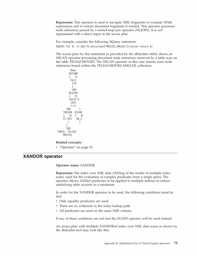
Represents: This operator is used to navigate XML fragments to evaluate XPath
expressions and to extract document fragments if needed. This operator processes
node references passed by a nested-loop join operator (NLJOIN). It is not
represented with a direct input in the access plan.
For example, consider the following XQuery statement:
XQUERY for $i in db2-fn:xmlcolumn("MOVIES.XMLCOL")//actor return $i
The access plan for this statement as provided by the db2exfmt utility shows an
XSCAN operator processing document node references retrieved by a table scan on
the table TELIAZ.MOVIES. The XSCAN operator in this case returns actor node
references found within the TELIAZ.MOVIES.XMLCOL collection.
Rows
RETURN
( 1)
Cost
I/O
|
180
NLJOIN
( 2)
10137.9
1261
/-+\
180 1
TBSCAN XSCAN
( 3) ( 4)
21.931 56.2
1 7
|
180
TABLE: TELIAZ
MOVIES
Related concepts:
v “Operator” on page 52
XANDOR operator
Operator name: XANDOR
Represents: The index over XML data ANDing of the results of multiple index
scans, used for the evaluation of complex predicates from a single query. The
operator allows ANDed predicates to be applied to multiple indexes to reduce
underlying table accesses to a minimum.
In order for the XANDOR operator to be used, the following conditions must be
met:
v Only equality predicates are used.
v There are no wildcards in the index lookup path.
v All predicates are used on the same XML column.
If any of these conditions are not met the IXAND operator will be used instead.
An access plan with multiple XANDORed index over XML data scans as shown by
the db2exfmt tool may look like this:
Appendix B. Alphabetical list of Visual Explain operators 73

Rows
RETURN
( 1)
Cost
I/O
|
0.00915933
NLJOIN
( 2)
985.789
98.9779
/--+--\
2.96215 0.00309213
FETCH XSCAN
( 3) ( 11)
340.113 217.976
19 27
/---+---\
2.96215 210000
RIDSCN TABLE: DB2XML
( 4) TPCHX
332.008
18
|
2.96215
SORT
( 5)
331.957
18
|
2.96215
XANDOR
( 6)
331.784
18
+----------------+--------+-------+----------------+
355.62 6996.81 105000 105000
XISCAN XISCAN XISCAN XISCAN
( 7) ( 8) ( 9) ( 10)
165.892 3017.54 1.6473e+06 851554
9 81 27768 14898
| | | |
210000 210000 210000 210000
XMLIN: DB2XML XMLIN: DB2XML XMLIN: DB2XML XMLIN: DB2XML
TPCHX_IDX TPCHX_IDX TPCHX_IDX TPCHX_IDX
Each XISCAN operator will perform an index scan and feed the XANDOR
operator with the XML node IDs that qualify. The XANDOR operator will apply
the AND and OR predicates and return the XML nodes that satisfy the XML
pattern for the query.
Performance suggestions:
v Over time, database updates may cause an index to become fragmented,
resulting in more index pages than necessary. This can be corrected by dropping
and recreating the index, or by reorganizing it.
v If statistics are not current, update them using the RUNSTATS command.
v In general, index scans are most effective when only a few rows qualify. To
estimate the number of qualifying rows, the optimizer uses the statistics that are
available for the columns referenced in predicates. If some values occur more
frequently than others, it is important to request distribution statistics by using
the WITH DISTRIBUTION clause with the RUNSTATS command. By using
the non-uniform distribution statistics, the optimizer can distinguish among
frequently and infrequently occurring values.
74 Visual Explain Tutorial

Related concepts:
v “Operator” on page 52
Appendix B. Alphabetical list of Visual Explain operators 75

76 Visual Explain Tutorial

Appendix C. DB2 concepts
v Databases
v Schemas
v Tables
Databases
A relational database presents data as a collection of tables. A table consists of a
defined set of columns and any number of rows. The data in each table is logically
related, and relationships can be defined between tables. Data can be viewed and
manipulated based on mathematical principles and operations called relations
(such as, INSERT, SELECT, and UPDATE).
A database is self-describing in that it contains, in addition to data, a description of
its own structure. It includes a set of system catalog tables, which describe the
logical and physical structure of the data; a configuration file, which contains the
parameter values associated with the database; and a recovery log, which records
ongoing transactions and transactions that can be archived.
Databases can be local or remote. A local database is physically located on the
workstation in use, while a database on another machine is considered remote.
Related concepts:
v “Visual Explain overview” in Administration Guide: Implementation
Schemas
A schema is a unique identifier used to group a set of database objects (such as,
tables, views, indexes, and aliases). That is, if you were creating a table named
PAYROLL, it would be tedious to have to search the database to find out whether
some other user has already created a table with the same name. The name of each
object needs to be unique only within its schema.
Most database objects have a two-part object name, the first part being the schema
name and the second part is the name of the object. When an object is created, you
can assign it to a specific schema. If you do not specify a schema, it is assigned to
the default schema, which is usually the user ID of the person who created the
object. For example, a user named Smith might have a table named
SMITH.PAYROLL.
The schema also becomes an object in the database. It is created when the first
object in the schema is created. A schema can be owned by an individual, and the
owner can control access to the data and the objects within it.
Related concepts:
v “Visual Explain overview” in Administration Guide: Implementation
© Copyright IBM Corp. 2002, 2006 77

Tables
A relational database presents data as a collection of tables. A table consists of data
logically arranged in columns and rows (generally known as records).
Each table has a name, and within a table, each column has a name. No particular
ordering is maintained among the rows of a table, but rows can be retrieved in an
order determined by values in their columns. The data in a table is logically
related. All database and table data is assigned to table spaces.
Related concepts:
v “Visual Explain overview” in Administration Guide: Implementation
78 Visual Explain Tutorial

Appendix D. Additional information
v Guidelines for creating indexes
v Out-of-date access plans
v Using runstats
Guidelines for creating indexes
Creating appropriate indexes allows the optimizer to choose an index scan for
those cases where it would be more efficient than a table scan.
Some guidelines for creating indexes include:
v Define primary keys and unique indexes wherever they apply.
v Create an index on any column that the query uses to join tables (join
predicates).
v Create an index on any column from which you search for particular values on a
regular basis.
v Create an index on columns that are commonly used in ORDER BY clauses.
v Ensure that you have used predicates that retrieve only the data you need. For
example, ensure that the selectivity value for the predicates represents the
portion of the table that you want returned.
v When creating a multicolumn index, the first columns of the index should be the
ones that are used most often by the predicates in your query.
v Ensure that the disk and update maintenance overhead an index introduces will
not be too high.
Related concepts:
v “Space requirements for indexes” in Administration Guide: Planning
v “Visual Explain overview” in Administration Guide: Implementation
Related tasks:
v “Estimating space requirements for tables and indexes” in Administration Guide:
Implementation
Out-of-date access plans
Symptom
The STATS_TIME row indicates that the statistics are not updated.
Possible cause
The optimizer used default values. (These default values are displayed
with the keyword ″default″.) This situation can result in an out-of-date
access plan.
Action
It is recommended that you use the runstats command to update the
statistics; then rebind the package.
Related concepts:
v “Access plan” on page 47
v “Visual Explain overview” in Administration Guide: Implementation
© Copyright IBM Corp. 2002, 2006 79
Using RUNSTATS
The optimizer uses the catalog tables from a database to obtain information about
the database, the amount of data in it, and other characteristics, and uses this
information to choose the best way to access the data. If current statistics are not
available, the optimizer might choose an inefficient access plan based on inaccurate
default statistics.
It is highly recommended that you use the RUNSTATS command to collect current
statistics on tables and indexes, especially if significant update activity has
occurred or new indexes have been created since the last time the RUNSTATS
command was executed. This provides the optimizer with the most accurate
information with which to determine the best access plan.
Be sure to use RUNSTATS after making your table updates; otherwise, the table
might appear to the optimizer to be empty. This problem is evident if cardinality
on the Operator Details window equals zero. In this case, complete your table
updates, rerun the RUNSTATS command and recreate the explain snapshots for
affected tables.
Note:
v Use RUNSTATS on all tables and indexes that might be accessed by a query.
v The quantile and frequent value statistics determine when data is unevenly
distributed. To update these values, use RUNSTATS on a table with the WITH
DISTRIBUTION clause.
v In addition to statistics, other factors (such as the ordering of qualifying rows,
table size, and buffer pool size) might influence how an access plan is selected.
v Applications should be rebound (and their statements optionally re-explained)
after you run the RUNSTATS command or change configuration parameters.
The RUNSTATS command (which can be entered from the DB2 CLP prompt) can
provide different levels of statistics as shown in the following syntax:
Basic Statistics
Table:
RUNSTATS ON TABLE tablename
Index:
RUNSTATS ON TABLE tablename FOR INDEXES ALL
Both tables and indexes:
RUNSTATS ON TABLE tablename AND INDEXES ALL
Enhanced Statistics
Table:
RUNSTATS ON TABLE tablename WITH DISTRIBUTION
Index:
RUNSTATS ON TABLE tablename FOR DETAILED INDEXES ALL
Both tables and indexes:
RUNSTATS ON TABLE tablename WITH DISTRIBUTION AND
DETAILED INDEXES ALL
80 Visual Explain Tutorial

Note: In each of the above commands, the tablename must be fully qualified with
the schema name.
Related concepts:
v “Visual Explain overview” in Administration Guide: Implementation
Related reference:
v “RUNSTATS command” in Command Reference
Appendix D. Additional information 81

82 Visual Explain Tutorial

Appendix E. Notices
IBM® may not offer the products, services, or features discussed in this document
in all countries. Consult your local IBM representative for information on the
products and services currently available in your area. Any reference to an IBM
product, program, or service is not intended to state or imply that only that IBM
product, program, or service may be used. Any functionally equivalent product,
program, or service that does not infringe any IBM intellectual property right may
be used instead. However, it is the user’s responsibility to evaluate and verify the
operation of any non-IBM product, program, or service.
IBM may have patents or pending patent applications covering subject matter
described in this document. The furnishing of this document does not give you
any license to these patents. You can send license inquiries, in writing, to:
IBM Director of Licensing
IBM Corporation
North Castle Drive
Armonk, NY 10504-1785
U.S.A.
For license inquiries regarding double-byte (DBCS) information, contact the IBM
Intellectual Property Department in your country/region or send inquiries, in
writing, to:
IBM World Trade Asia Corporation
Licensing
2-31 Roppongi 3-chome, Minato-ku
Tokyo 106, Japan
The following paragraph does not apply to the United Kingdom or any other
country/region where such provisions are inconsistent with local law:
INTERNATIONAL BUSINESS MACHINES CORPORATION PROVIDES THIS
PUBLICATION “AS IS” WITHOUT WARRANTY OF ANY KIND, EITHER
EXPRESS OR IMPLIED, INCLUDING, BUT NOT LIMITED TO, THE IMPLIED
WARRANTIES OF NON-INFRINGEMENT, MERCHANTABILITY, OR FITNESS
FOR A PARTICULAR PURPOSE. Some states do not allow disclaimer of express or
implied warranties in certain transactions; therefore, this statement may not apply
to you.
This information could include technical inaccuracies or typographical errors.
Changes are periodically made to the information herein; these changes will be
incorporated in new editions of the publication. IBM may make improvements
and/or changes in the product(s) and/or the program(s) described in this
publication at any time without notice.
Any references in this information to non-IBM Web sites are provided for
convenience only and do not in any manner serve as an endorsement of those Web
sites. The materials at those Web sites are not part of the materials for this IBM
product, and use of those Web sites is at your own risk.
IBM may use or distribute any of the information you supply in any way it
believes appropriate without incurring any obligation to you.
© Copyright IBM Corp. 2002, 2006 83

Licensees of this program who wish to have information about it for the purpose
of enabling: (i) the exchange of information between independently created
programs and other programs (including this one) and (ii) the mutual use of the
information that has been exchanged, should contact:
IBM Canada Limited
Office of the Lab Director
8200 Warden Avenue
Markham, Ontario
L6G 1C7
CANADA
Such information may be available, subject to appropriate terms and conditions,
including in some cases payment of a fee.
The licensed program described in this document and all licensed material
available for it are provided by IBM under terms of the IBM Customer Agreement,
IBM International Program License Agreement, or any equivalent agreement
between us.
Any performance data contained herein was determined in a controlled
environment. Therefore, the results obtained in other operating environments may
vary significantly. Some measurements may have been made on development-level
systems, and there is no guarantee that these measurements will be the same on
generally available systems. Furthermore, some measurements may have been
estimated through extrapolation. Actual results may vary. Users of this document
should verify the applicable data for their specific environment.
Information concerning non-IBM products was obtained from the suppliers of
those products, their published announcements, or other publicly available sources.
IBM has not tested those products and cannot confirm the accuracy of
performance, compatibility, or any other claims related to non-IBM products.
Questions on the capabilities of non-IBM products should be addressed to the
suppliers of those products.
All statements regarding IBM’s future direction or intent are subject to change or
withdrawal without notice, and represent goals and objectives only.
This information may contain examples of data and reports used in daily business
operations. To illustrate them as completely as possible, the examples include the
names of individuals, companies, brands, and products. All of these names are
fictitious, and any similarity to the names and addresses used by an actual
business enterprise is entirely coincidental.
COPYRIGHT LICENSE:
This information may contain sample application programs, in source language,
which illustrate programming techniques on various operating platforms. You may
copy, modify, and distribute these sample programs in any form without payment
to IBM for the purposes of developing, using, marketing, or distributing
application programs conforming to the application programming interface for the
operating platform for which the sample programs are written. These examples
have not been thoroughly tested under all conditions. IBM, therefore, cannot
guarantee or imply reliability, serviceability, or function of these programs.
Each copy or any portion of these sample programs or any derivative work must
include a copyright notice as follows:
84 Visual Explain Tutorial

© (your company name) (year). Portions of this code are derived from IBM Corp.
Sample Programs. © Copyright IBM Corp. _enter the year or years_. All rights
reserved.
Trademarks
Company, product, or service names identified in the documents of the DB2
Version 9 documentation library may be trademarks or service marks of
International Business Machines Corporation or other companies. Information on
the trademarks of IBM Corporation in the United States, other countries, or both is
located at http://www.ibm.com/legal/copytrade.shtml.
The following terms are trademarks or registered trademarks of other companies
and have been used in at least one of the documents in the DB2 documentation
library:
Microsoft®, Windows®, Windows NT®, and the Windows logo are trademarks of
Microsoft Corporation in the United States, other countries, or both.
Intel®, Itanium®, Pentium®, and Xeon® are trademarks of Intel Corporation in the
United States, other countries, or both.
Java™ and all Java-based trademarks are trademarks of Sun Microsystems, Inc. in
the United States, other countries, or both.
UNIX® is a registered trademark of The Open Group in the United States and
other countries.
Linux® is a trademark of Linus Torvalds in the United States, other countries, or
both.
Other company, product, or service names may be trademarks or service marks of
others.
Appendix E. Notices 85

86 Visual Explain Tutorial

Index
Aaccess plan
collecting current statisticsin a partitioned database
environment 34
in a single-partition database
environment 17
creating additional indexesin a partitioned database
environment 42
in a single-partition database
environment 26
creating indexes on columns used to
join tablesin a partitioned database
environment 38
in a single-partition database
environment 21
improvingin a partitioned database
environment 31
in a single-partition database
environment 13
query with no indexes and no
statisticsin a partitioned database
environment 32
in a single-partition database
environment 14
access plan graph 48
changing appearance 10
for a list of previously explained SQL
or XQuery statements 7
getting more details 9
magnifying 8
reading the symbols 7
access plan graph node 49
access plansout-of-date 79
overview 47
Cclustering
definition 49
CMPEXP operatordescription 61
commandsEXPLAIN.DDL 3
vesampl.ddl 3
contacting IBM 89
containersdefinition 49
costdefinition 50
CREATE INDEX statementoverview 79
creatingindexes 79
cursor blockingdefinition 50
Ddatabase-managed table spaces
definition 50
databasesdefinition 77
DELETE operatordefinition 62
dynamic SQL or XQuery statementsdefinition 51
EEISCAN operator
definition 62
explain snapshotdefinition 51
explain snapshotsfor dynamic SQL or XQuery
statements 5
for static SQL or XQuery
statements 6
for Visual Explain tutorial 3
explain tablescreating 3
EXPLAIN.DDLcommand 3
explainable statementsdefinition 52
explained SQL statementsdefinition 52
explained XQuery statementsdefinition 52
explsnap option 6
FFETCH operator
definition 62
FILTER operatordefinition 63
GGENROW operator
definition 63
GRPBY operatordefinition 63
HHSJOIN operator
definition 64
Iindexes
creation 79
indexes on table columnscreating
in a partitioned database
environment 42
INSERT operatordefinition 64
IXAND operatordefinition 65
IXSCAN operatordefinition 65
MMSJOIN operator
definition 66
NNLJOIN operator
definition 66
notices 83
Ooperand
definition 52
operatorsCMPEXP 61
definition 52
DELETE 62
EISCAN 62
FETCH 62
FILTER 63
GENROW 63
GRPBY 63
HSJOIN 64
INSERT 64
IXAND 65
IXSCAN 65
MSJOIN 66
NLJOIN 66
PIPE 67
RETURN 67
RIDSCN 67
RPD 68
SHIP 68
SORT 68
TBSCAN 69
TEMP 70
TQUEUE 70
UNION 70
UNIQUE 71
UPDATE 71
XANDOR 73
XISCAN 71
XSCAN 72
© Copyright IBM Corp. 2002, 2006 87

optimizerdefinition 54
Ppackages
definition 54
PIPE operatordefinition 67
predicatedefinition 55
Qquery optimization class
definition 55
RRETURN operator
definition 67
RIDSCN operatordefinition 67
row blockingsee cursor blocking 50
RPD operatordefinition 68
runstatsusing 80
Sschemas
definition 77
selectivity of predicatesdefinition 56
SHIP operatordefinition 68
SORT operatordefinition 68
star joinsdefinition 57
static SQL or XQuery statementsdefinition 58
system-managed table spacesdefinition 58
Ttable spaces
definition 58
tablesdefinition 78
TBSCAN operatordefinition 69
TEMP operatordefinition 70
timeronsabout 59
TQUEUE operatordefinition 70
tutorialsVisual Explain 1
UUNION operator
definition 70
UNIQUE operatordefinition 71
UPDATE operatordefinition 71
Vvesampl.ddl command 3
Visual Explainaccess plan graph 48
access plans 47
definition 59
tutorial 1
XXANDOR operator
definition 73
XISCAN operatordefinition 71
XSCAN operatordefinition 72
88 Visual Explain Tutorial

Contacting IBM
To contact IBM in your country or region, check the IBM Directory of Worldwide
Contacts at http://www.ibm.com/planetwide
To learn more about DB2 products, go to
http://www.ibm.com/software/data/db2/.
© Copyright IBM Corp. 2002, 2006 89

90 Visual Explain Tutorial


����
Printed in USA
SC10-4319-00