day 3 prevalence 1. on an average school day, how many hours do you watch tv? a. i do not watch tv...

Day 3

Prevalence

1

On an average school day, how many hours do you watch TV?

A. I do not watch TV on an average school day

B. Less than 1 hour per day

C. 1 hour per day

D. 2 hours per day

E. 3 hours per day

F. 4 hours per day

G. 5 or more hours per day

✔ From questions to answers

✔ From answers to counts

From counts to prevalence

From prevalence to statements

Continuing with Tools for Doing the Study

2

✔What are you curious about?

✔From curiosity to a hypothesis

✔From a hypothesis to questions

✔From questions to answers

✔From answers to counts

From counts to prevalence

From prevalence to statements

Interpretation – Conclusions - Communication

3

Continuing with tools for doing a study

4

Three main tools

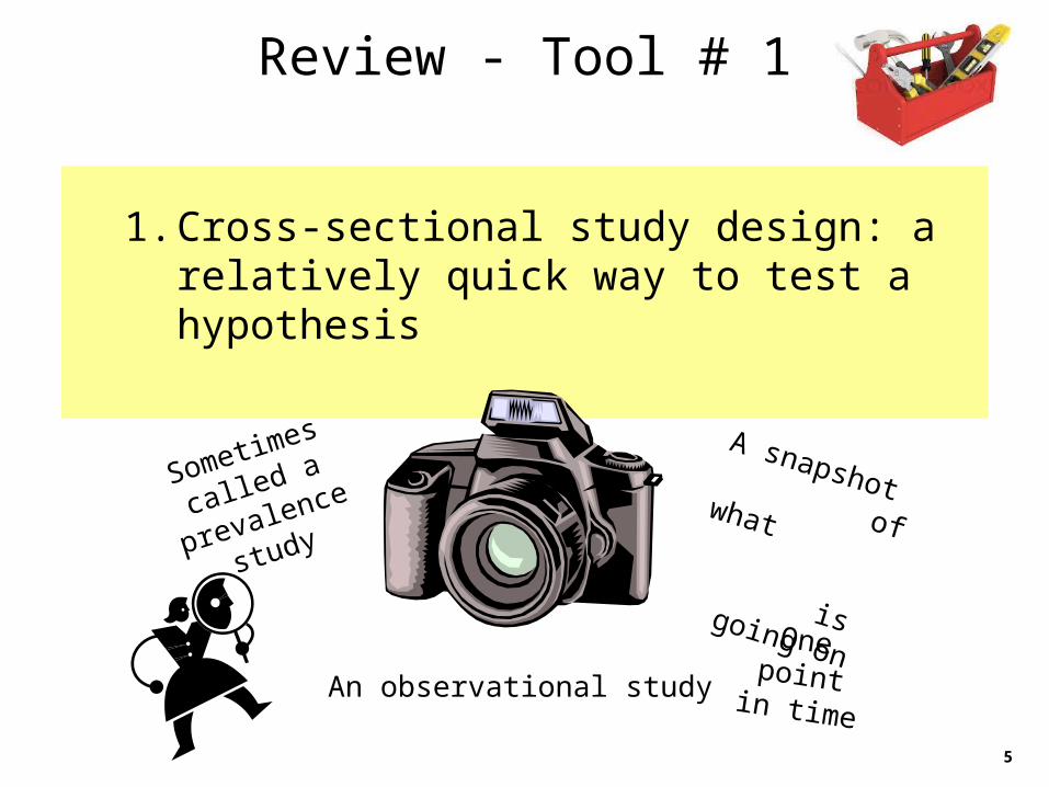
1. Cross-sectional study design: a relatively quick way to test a hypothesis

5

Review - Tool # 1

An observational study

A snapshot of what is going on

Sometimes called a

prevalence study

One point in time

2. Contingency table: puts numbers in a table so we can get from answers to counts

6

Review - Tool # 2

Handy for calculations

The simplest table is the 2x2 table

Shows exposure

and outcome

Everyone is in the table somewhere

3. Prevalence – calculations to quantify outcomes in populations; prevalence ratios (comparisons) provide a measure of association between exposure and outcome

7

Tool # 3

Everyone with the

outcome – recent

and long-term

Calculated as

a fraction or

percentage

Especially used in cross-sectional studies

From Epi Textbooks

The main outcome measure obtained from a cross-sectional study is prevalence.

A cross-sectional study is sometimes called a prevalence study.

8

9

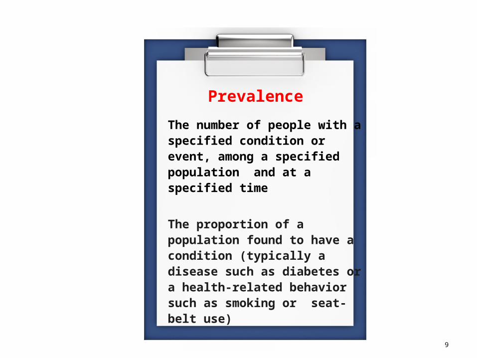
The number of people with a specified condition or event, among a specified population and at a specified time

The proportion of a population found to have a condition (typically a disease such as diabetes or a health-related behavior such as smoking or seat-belt use)

Prevalence

The Numerator is the number of people in the population or sample who experienced the outcome or effect, in this case, wearing blue.

11

Express it in numbers

The Denominator is the total number of people in the population or sample, in this case, total number of students in the class.

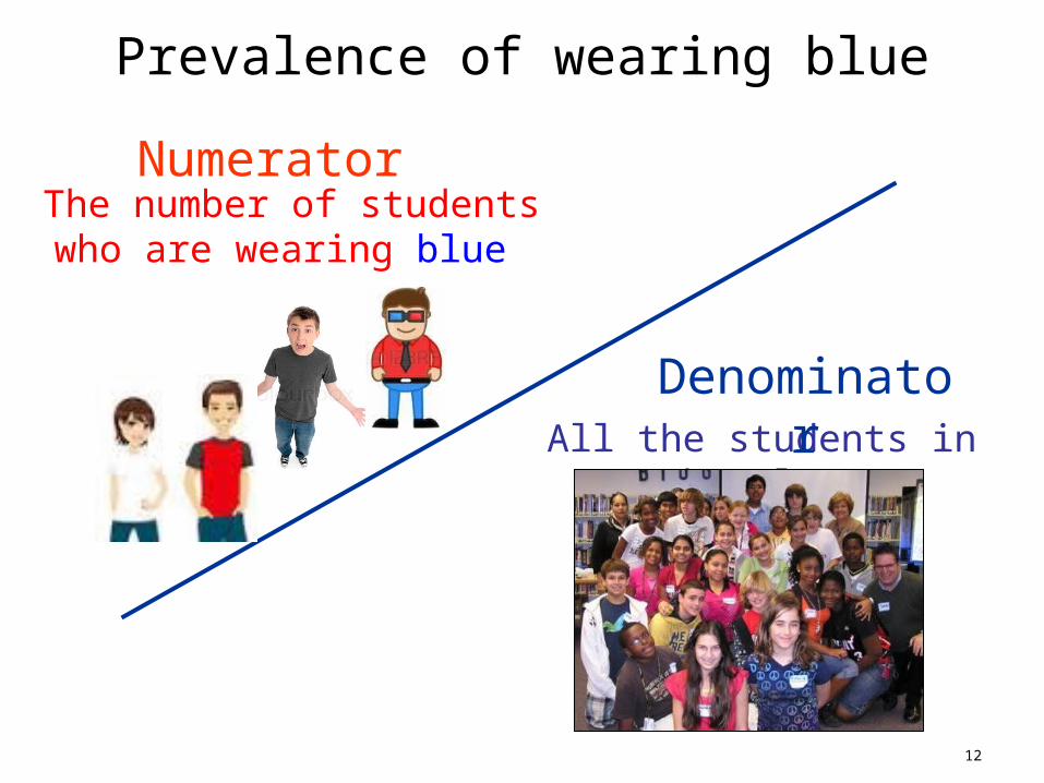
Prevalence of wearing blue

The number of students who are wearing blue

All the students in the class

Numerator

Denominator

12

Prevalence of wearing blue

13

# wearing blue # in class x 100 = % wearing blue

= Prevalence

Prevalence of wearing glasses

All the students in the classDenominator

14

The number of students who are wearing glasses

Numerator

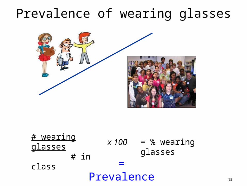
Prevalence of wearing glasses

15

# wearing glasses # in class x 100 = % wearing glasses

= Prevalence

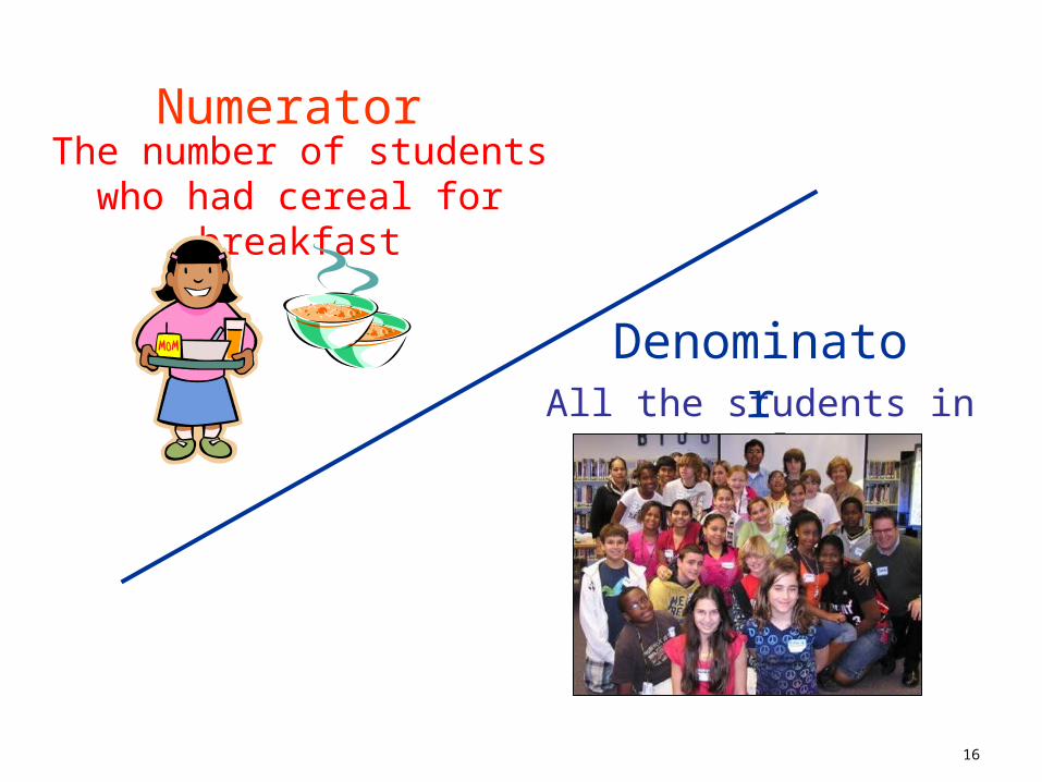
The number of students who had cereal for breakfast


Numerator

Denominator

16

17

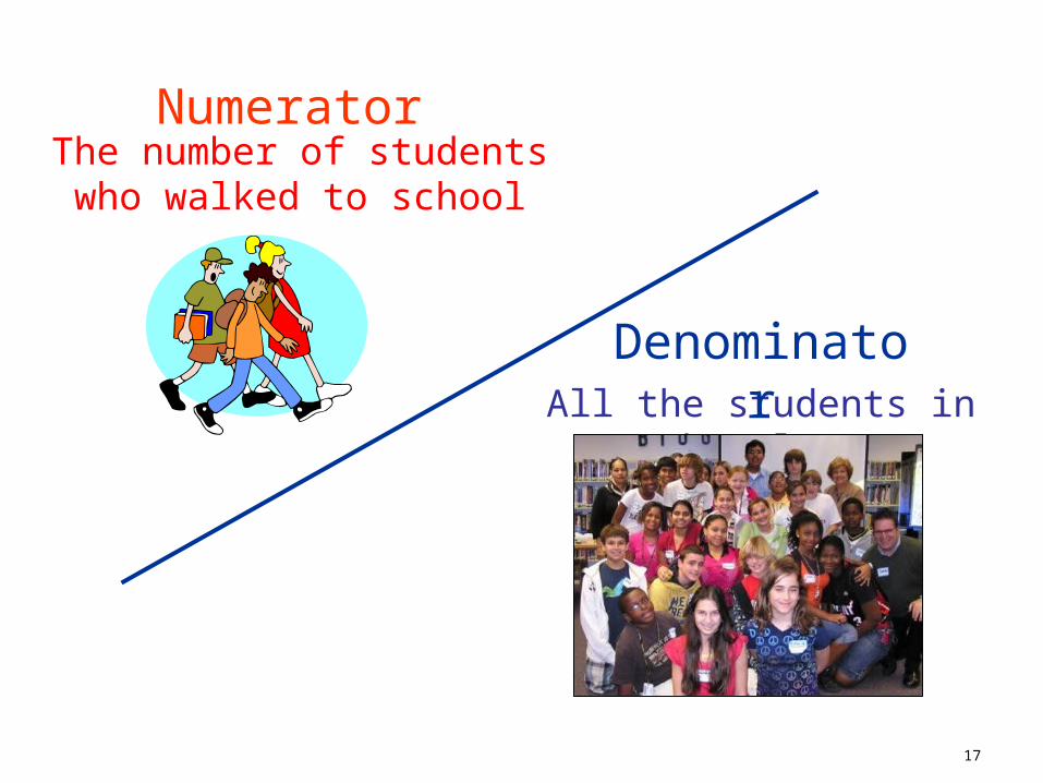
The number of students who walked to school

Numerator


Denominator

18

The number of students who . . . ? Numerator


Denominator

19

Prevalence Ratio

A comparison of two

prevalences

Calculated by dividing the

prevalence of the outcome

in the exposed by the

prevalence of the outcome

in the unexposed

a/(a+b) divided by c/(c+d).

People who ____________________________________________

are ______ times as likely to _______________________________

compared to people who __________________________________ 20

30

100

30 %30 70 100 a b

c d

Hyper-texter

Not a hyper-texter

TotalBinge drinker

Not a binge drinker Prevalence

88

400

22 %88 312 400

Prevalence Ratio

1.4

÷ a a+b

c c + d

High school students who send more text messages/day are more likely to binge drink compared to students who send fewer text messages/day.

21

30

100

30 %30 70 100 a b

c d

Hyper-texter

Not a hyper-texter

TotalBinge drinker

Not a binge drinker Prevalence

88

400

22 %88 312 400

Prevalence Ratio

1.4

High school students who send more text messages/day are more likely to binge drink compared to students who send fewer text messages/day.

Hyper-texters are 1.4 times as likely to binge drink than

those who are not hyper-texters.

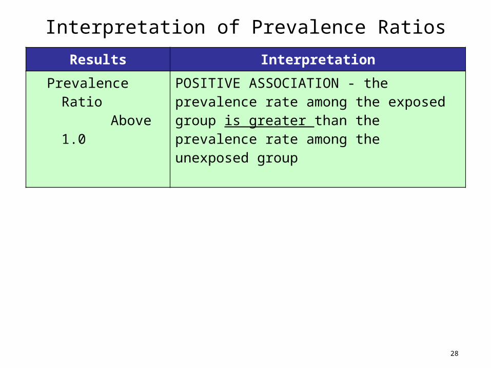
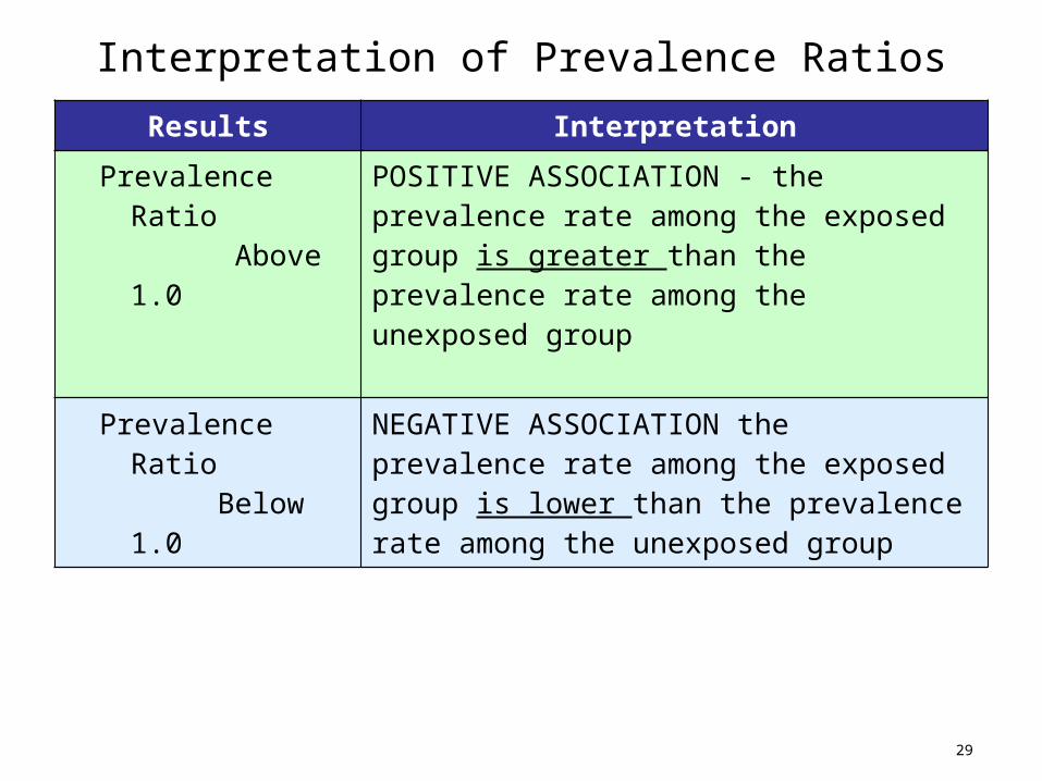
Interpretation of Prevalence Ratios

22

Results Interpretation

Prevalence Ratio Above 1.0

POSITIVE ASSOCIATION - the prevalence rate among the exposed group is greater than the prevalence rate among the unexposed group

People who ____________________________________________



656

1427

46 %656 771 1427 a b

c d

No restriction

Partial or complete restriction

TotalTried smoking

Did not try smoking Prevalence

413

3117

13%413 2704 3117

Prevalence Ratio

3.5

÷ a a+b

c c + d

Teenagers who are not restricted from watching R-rated films are more likely to try smoking compared to teenagers who have restrictions on watching R-rated films.

24

656

1427

46 %656 771 1427 a b

c d

No restriction

Partial or complete restriction

TotalTried smoking

Did not try smoking Prevalence

413

3117

13%413 2704 3117

Prevalence Ratio

3.5

Teenagers who have no restrictions on watching R-rated

films are 3.5 times as likely to try smoking as those who

have restrictions.

Teenagers who are not restricted from watching R-rated films are more likely to try smoking compared to teenagers who have restrictions on watching R-rated films.


25




People who ____________________________________________



95

1000

9.5 %95 905 1000 a b

c d

Urban

Rural

Total

Did Experiment

Did not experiment Prevalence

130

1000

13.0 %130 870 1000

Prevalence Ratio

0.73

÷ a a+b

c c + d

Students living in urban areas engage in more experimenting with prescription drugs than students living in rural areas.

27

95

1000

9.5 %95 905 1000 a b

c d

Urban

Rural

TotalExperiment Did not experiment Prevalence

130

1000

13.0 %130 870 1000

Prevalence Ratio

0.73

Students living in urban areas engage in more experimenting with prescription drugs than students living in rural areas.

Students in urban areas are 0.73 times as likely to experiment

with prescription drugs than students in rural areas.


28





29




Prevalence Ratio Below 1.0

NEGATIVE ASSOCIATION the prevalence rate among the exposed group is lower than the prevalence rate among the unexposed group


30




Prevalence Ratio Below 1.0

NEGATIVE ASSOCIATION the prevalence rate among the exposed group is lower than the prevalence rate among the unexposed group

Prevalence Ratio At or Near 1.0

NO ASSOCIATION – the prevalence rate among the exposed group is similar or the same as the prevalence rate among the unexposed group

• A prevalence ratio of 1.1 is a weak positive association, while a prevalence ratio of 3.1 is a strong positive association

• A prevalence ratio of 0.95 is a weak negative association, while a ratio of 0.45 is a strong negative association

31

Results from some Epi Teams in Paterson NJ

Epi Stars - Drinking at least 2 cans or a 20-ounce bottle of non-diet soda every day leads to a crash (feeling tired) - PR = 2.5

Pop Science – A healthy breakfast is associated with playing in an organized sport - PR = 0.96

Hypertensions – Receiving a daily, weekly, or monthly allowance is related to eating junk food/unhealthy food more than twice a day - PR = 1.6

Dr. Observation – Healthy eating (at least 2 servings of fruit and vegetables a day) results in better grades (“doing well in school”) - PR = 1.0

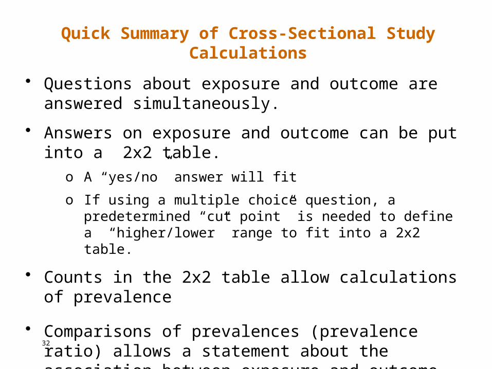
Quick Summary of Cross-Sectional Study Calculations

• Questions about exposure and outcome are answered simultaneously.

• Answers on exposure and outcome can be put into a 2x2 table.

o A “yes/no” answer will fit

o If using a multiple choice question, a predetermined “cut point” is needed to define a “higher/lower” range to fit into a 2x2 table.

• Counts in the 2x2 table allow calculations of prevalence

• Comparisons of prevalences (prevalence ratio) allows a statement about the association between exposure and outcome.

32

The prevalence ratio (PR) is a measure of risk used in cross-sectional studies. It compares prevalence in the exposed to prevalence in the unexposed. A ratio of 1.0 denotes no difference between the two groups.

Measure of Risk E

xam

ple

s

Interpreting SMR and Confidence Intervals

0 1 2 3 4 5 6 7

Low, Statistically Significant

As Expected

High, Not Statistically Significant

High, Statistically Significant

SMRBaselineMortality

in GeneralPopulation

Interpreting PR and Confidence Intervals

Prevalence RatioNo difference between

exposed and unexposed

Breakout Assignment

Prevalence

34

35

Perform a few practice calculations as needed

36

Calculate the prevalence of the outcome – for the exposed group and for the unexposed group.

Calculate the prevalence ratio.

Populate the 2x2 table on page 1 with the above information.

Make a statement that uses the prevalence ratio to describe size of the association.

Deck Worksheet – page 2

37

Study Proposal: Section 6

6. Data Analysis Plan

6a. Contingency Table

6b. Prevalence among exposed

6c. Prevalence among unexposed

6d. Prevalence Ratio

6e. Statement of results

6f. How prevalence ratio will be used in your study

day 3 prevalence 1. on an average school day, how many hours do you watch tv? a. i do not watch tv...

Documents