david michael mohr - usq eprintseprints.usq.edu.au/22590/1/mohr_2011.pdf · irrigation machines and...
TRANSCRIPT

University of Southern Queensland
Faculty of Engineering and Surveying
Performance Characterisation of Pressure Regulation Devices used in
Broad-Acre Irrigation
A dissertation submitted by
David Michael Mohr
In fulfilment of the requirements of
Courses ENG4111 and ENG4112 Research Project
towards the degree of
Bachelor of Engineering (Agricultural)
Submitted: October 2011
Performance Characterisation of Pressure Regulation Devices Used in Broad-Acre Irrigation
Page i
ABSTRACT
Large mobile irrigation machines are becoming a common sight in Australian broad-
acre irrigation, replacing traditional surface methods. These machines give the potential
of irrigating large areas with high efficiency and with a uniformity of above 80% when
designed correctly.
A major component of the large mobile irrigation machine is the sprinkler application
package commissioned with the machine. Pressure regulators are becoming a common
part of the package when large mobile irrigation machines are commissioned.
Pressure regulators are installed upstream of the nozzle and provide a constant output
pressure regardless of the input pressure into the pressure regulator. The device acts as a
variable headloss. Input pressure changes are a common occurrence on large mobile
irrigation machines and typically are from topographic changes as the machines travel
through the field.
The application rate is directly influenced by the output pressure from the pressure
regulator, thus this shows the importance of accurately understanding to performance of
the pressure regulator. Reviewing previous literature it was known that the methodology
development was a crucial part in understanding the pressure regulator performance.
The development of a solid robust methodology was the primary objective of this
dissertation.
Eight stages of testing occurred each with incremental changes to develop the
methodology for testing. The way the testing was undertaking proved to influence the
results of the test.
A statistical analysis in terms of an ANOVA and sample size calculations was
undertaken on a limited set of data. It was found the for the 16 pressure regulators tested

Performance Characterisation of Pressure Regulation Devices Used in Broad-Acre Irrigation
Page ii
the means were not equal. 88 pressure regulators were found to be tested to understand
manufacturing variation based on the normal model.
The methodology by which the test was carried out was found to influence the outcome
of the pressure regulator. Each result needs to be interpreted with reference to the
methodology. Much more testing is needed to fully understand the pressure regulators
performance and how they function on large mobile irrigation machines.
Performance Characterisation of Pressure Regulation Devices Used in Broad-Acre Irrigation
Page iii
University of Southern Queensland
Faculty of Engineering and Surveying
ENG4111 Research Project Part 1 &
ENG4112 Research Project Part 2
LIMITATIONS OF USE
The Council of the University of Southern Queensland, its Faculty of Engineering and Surveying, and the staff of the University of Southern Queensland, do not accept any responsibility for the truth, accuracy or completeness of material contained within or associated with this dissertation.
Persons using all or any part of this material do so at their own risk, and not at the risk of the Council of the University of Southern Queensland, its Faculty of Engineering and Surveying or the staff of the University of Southern Queensland.
This dissertation reports an educational exercise and has no purpose or validity beyond this exercise. The sole purpose of the course pair entitled “Research Project” is to contribute to the overall education within the student's chosen degree program. This document, the associated hardware, software, drawings, and other material set out in the associated appendices should not be used for any other purpose: if they are so used, it is entirely at the risk of the user.
Professor Frank Bullen
Dean
Faculty of Engineering and Surveying

Performance Characterisation of Pressure Regulation Devices Used in Broad-Acre Irrigation
Page iv
CERTIFICATION OF DISSERTATION
I certify that the ideas, designs and experimental work, results, analyses and conclusions set out in this dissertation are entirely my own effort, except where otherwise indicated and acknowledged.
I further certify that the work is original and has not been previously submitted for assessment in any other course or institution, except where specifically stated.
Student Name: DAVID M MOHR
Student Number: 0050086160
____________________________
Signature
____________________________
Date

Performance Characterisation of Pressure Regulation Devices Used in Broad-Acre Irrigation
Page v
ACKNOWLEDGEMENTS
Firstly and above all I must thank the Lord, as without him, all is in vein.
To my project supervisor and the originator of this project, Dr. Joseph Foley. Words
cannot express the thanks I have for your patience, mentoring, support, technical
guidance and ideas over the past 12 months. This project has been an immense learning
experience and for this I thank-you.
To the technical and workshop staff from whom I borrowed countless tools, made
components on short notice and answered the endless questions I had about the
equipment, I thank you. Particular acknowledgement should be given to Dean Beliveau,
Chris Galligan, Brian Aston and Daniel Eising.
I acknowledge the funding which has been provided for this project, by the National
Centre for Engineering in Agriculture.
To my mates, Ben and Tyronne who helped me with the level run survey, thank-you
blokes.
Finally to my Parents, the love, support and encouragement you have given me for this
project and over the last four years to complete this degree, thank-you. I am forever in
debt to you.
Performance Characterisation of Pressure Regulation Devices Used in Broad-Acre Irrigation
Page vi
‘...it is not the quantity of water applied to a crop; it is the quantity
of intelligence applied which determines the results.’
Alfred Deakin 1890
Irrigation Pioneer to Australia

Performance Characterisation of Pressure Regulation Devices Used in Broad-Acre Irrigation
Page vii
TABLE OF CONTENTS
Abstract ......................................................................................................................... i
Limitations of Use ............................................................................................................ iii
Certification of Dissertation ............................................................................................. iv
Acknowledgements ........................................................................................................... v
Table of Contents ............................................................................................................ vii
List of Figures ................................................................................................................. xii
List of Tables................................................................................................................... xv
Chapter 1 Introduction ..................................................................................................... 1
1.1 Background ..................................................................................................... 1
1.2 Types of Irrigation .......................................................................................... 4
1.2.1 Surface Irrigation ................................................................................. 4
1.2.2 Pressurised Irrigation ........................................................................... 5
1.2.3 Large Mobile Irrigation Machines ....................................................... 7
1.2.4 Background to Large Mobile Irrigation Machines .............................. 8
1.2.5 Function of Large Mobile Irrigation Machines ................................. 10
1.3 Irrigation Performance .................................................................................. 11
1.4 Broad Aim..................................................................................................... 14
1.5 Objectives ..................................................................................................... 14
1.6 Structure of this Dissertation ........................................................................ 15
Chapter 2 Literature Review ......................................................................................... 16
2.1 Introduction ................................................................................................... 16
2.2 Flow Measurement ....................................................................................... 16
2.2.1 Flow measurement through pipes ...................................................... 16
2.3 Pressure Measurement .................................................................................. 18
Performance Characterisation of Pressure Regulation Devices Used in Broad-Acre Irrigation
Page viii
2.3.1 Pressure measurement through pipes ................................................. 18
2.4 Pressure Regulators Manufacturers .............................................................. 20
2.4.1 Nelson ................................................................................................ 20
2.4.2 Senninger ........................................................................................... 20
2.4.3 Rain Bird ............................................................................................ 21
2.4.4 Valley ................................................................................................. 21
2.4.5 Netafim .............................................................................................. 21
2.5 Pressure Regulators and Large Mobile Irrigation Machines ........................ 22
2.6 Previous Research ......................................................................................... 23
2.7 Statistical Analysis ........................................................................................ 35
2.7.1 Introduction ........................................................................................ 35
2.7.2 Statistical Methods and Analysis ....................................................... 36
2.7.3 Statistical Analysis described by Literature ....................................... 37
2.7.4 Analysis of Variance (ANOVA)........................................................ 38
2.8 Physical Analysis of Individual Components of Pressure Regulator ........... 41
2.8.1 Introduction ........................................................................................ 41
2.8.2 Spring ................................................................................................. 41
2.8.3 O-ring ................................................................................................. 43
Chapter 3 Materials and Methodology .......................................................................... 46
3.1 Introduction ................................................................................................... 46
3.2 Hydraulics Laboratory Experimental Setup ................................................. 46
3.2.1 Hydraulics Laboratory Constant Supply Header Tanks .................... 46
3.3 Test Rig and Kit ............................................................................................ 48
3.3.1 Introduction ........................................................................................ 48
3.3.2 Experiment Discharge Measurement ................................................. 48
3.3.3 Experiment Pressure Measurement ................................................... 48

Performance Characterisation of Pressure Regulation Devices Used in Broad-Acre Irrigation
Page ix
3.3.4 Experiment Pipes, Fittings and Valves .............................................. 49
3.3.5 Electronic Data Acquisition ............................................................... 50
3.3.6 Labview: The Data Acquisition Software ......................................... 50
3.4 Calibration of Electronic Measurement Devices .......................................... 51
3.4.1 Flowmeter Calibration ....................................................................... 51
3.4.2 Pressure Transducer Calibration ........................................................ 51
3.5 Function of the Nelson 10 PSI Pressure Regulator....................................... 58
3.6 Development of Testing Methodology ......................................................... 61
3.6.1 Introduction ........................................................................................ 61
3.6.2 Stage One – Result Replication from von Bernuth and Baird (1990) 61
3.6.3 Stage Two – Automatic data acquisition ........................................... 63
3.6.4 Stage Three – Automatic data acquisition with higher input heads .. 66
3.6.5 Stage Four – Continuing Valve Movement Test ............................... 68
3.7 Creep test ...................................................................................................... 69
3.8 Friction test ................................................................................................... 70
3.9 Displacement of Tube inside Pressure Regulator ......................................... 71
3.10 Statistical Analysis Testing Methodology ................................................ 76
Chapter 4 Results and Analysis ..................................................................................... 77
4.1 Introduction ................................................................................................... 77
4.2 Result Replication from von Bernuth and Baird (1990) ............................... 77
4.3 Automatic Data Acquisition ......................................................................... 81
4.4 Automatic data acquisition with higher input heads ..................................... 88
4.5 Continuing Hysteresis Tests ......................................................................... 95
4.6 Creep Test ..................................................................................................... 99
4.7 Friction Investigation .................................................................................. 102
4.8 Movement of Tube inside Pressure Regulator ............................................ 106
Performance Characterisation of Pressure Regulation Devices Used in Broad-Acre Irrigation
Page x
4.9 Statistical Analysis ...................................................................................... 111
4.9.1 Introduction ...................................................................................... 111
4.9.2 The ANOVA test ............................................................................. 111
4.9.3 Determination of Sample Size ......................................................... 114
Chapter 5 Discussion ................................................................................................... 115
5.1 Introduction ................................................................................................. 115
5.2 Result Replication from von Bernuth and Baird (1990) ............................. 115
5.2.1 Automatic Data Acquisition Test Results ........................................ 116
5.2.2 Automation Testing with Higher Input Pressures ........................... 117
5.3 Continuing Hysteresis Tests ....................................................................... 119
5.4 Creep Tests ................................................................................................. 121
5.5 Friction Investigation .................................................................................. 123
5.6 Displacement of Tube inside Pressure Regulator ....................................... 126
5.7 Statistical Analysis ...................................................................................... 128
5.7.1 ANOVA ........................................................................................... 128
5.7.2 Sample Size...................................................................................... 129
5.8 The Methodology and Model ..................................................................... 130
Chapter 6 Conclusions ................................................................................................. 131
Chapter 7 Recommendations For Future Work........................................................... 133
7.1 Introduction ................................................................................................. 133
7.2 Recommendations ....................................................................................... 133
Reference List ............................................................................................................... 135
Appendices .................................................................................................................... 140
Appendix A Project Specification .................................................................... 140
Appendix B Internal view of Nelson 10 PSI set pressure, pressure regulator with ¾ threaded female to ¾ square fitting ................................................................. 142

Performance Characterisation of Pressure Regulation Devices Used in Broad-Acre Irrigation
Page xi
Appendix C Table Z – Areas under the standard Normal curve ....................... 144
Appendix D Certificate of Calibration (flowmeter) .......................................... 146
Appendix E Level Run to Low and High Header tanks for pressure calibration 148
Appendix F Certificate of Calibration (Digital Multimeter used for Pressure Transducer Calibration) ....................................................................................... 150
Appendix G Labview output for Stage Two-Automatic data acquisition tests for discharges of 0.3 and 0.5 L/s ............................................................................... 152
Appendix H Matlab code for Stage two – Automatic data acquisition data processing 163
Appendix I Southern Cross Pump Curve HX-C Pump’s performance curve ... 180
Appendix J Labview output for Stage Three-Automatic data acquisition tests with higher heads for discharges of 0.3 and 0.6 L/s ............................................ 182
Appendix K Statistical Table – values of F for 5% significance level ............. 199

Performance Characterisation of Pressure Regulation Devices Used in Broad-Acre Irrigation
Page xii
LIST OF FIGURES
Figure 1.1 – Cotton under surface irrigation in Australia ................................................. 4
Figure 1.2 – Drip irrigation fixed under grape vines ........................................................ 6
Figure 1.3 – Cable tow travelling gun irrigator fed by flexible soft hose ......................... 7
Figure 1.4 – A 1250 metre Lateral Move in New South Wales ........................................ 8
Figure 1.5- The first large mobile irrigation machine ....................................................... 9
Figure 2.1 - Pressure Regulator and a LMIM ................................................................. 22
Figure 2.2 - Schematic of von Bernuth and Baird (1990) pressure regulator testrig ...... 24
Figure 2.3 – Typical pressure regulator performance as described in von Bernuth and Baird ................................................................................................................................ 25
Figure 2.4 – Single test results of Senninger 20 PSI pressure regulator at 0.47 L/s ....... 26
Figure 2.5 – Single test results of Nelson 20 PSI pressure regulator at 0.47 L/s ............ 26
Figure 2.6 – Single test results of Rainbird 20 PSI pressure regulator at 0.47 L/s ......... 27
Figure 2.7 – Performance of Senninger 6, 10, 15 and 20 PSI Pressure Regulators ........ 29
Figure 2.8 – Performance of Nelson 10, 15 and 20 PSI Pressure Regulators ................. 29
Figure 2.9 – Senninger 20 PSI Pressure Regulator at discharges 0.252, 0.504 and 0.756 L/s .................................................................................................................................... 30
Figure 2.10 – Senninger 15 PSI Pressure Regulator at discharges 0.252, 0.504 and 0.756 L/s .................................................................................................................................... 31
Figure 2.11 – Senninger 10 PSI Pressure Regulator at discharges 0.252, 0.504 and 0.756 L/s .................................................................................................................................... 31
Figure 2.13 – The Normal Model ................................................................................... 36
Figure 2.14 – Helical Compression Spring ..................................................................... 42
Figure 2.15 – Coil of a Helical Spring ............................................................................ 42
Figure 2.16 – O-ring Dimensions ................................................................................... 43
Figure 2.17 – Force Diagram .......................................................................................... 44

Performance Characterisation of Pressure Regulation Devices Used in Broad-Acre Irrigation
Page xiii
Figure 3.1 – Dead weight pressure tested calibrating the pressure transducers .............. 52
Figure 3.2 – Relationship between density and temperature for water ........................... 56
Figure 3.3 – Stage one testrig Results replication from von Bernuth and Baird (1990) . 63
Figure 3.4 – Stage two testrig Automatic data acquisition ............................................. 65
Figure 3.5 – Stage two testrig Automatic data acquisition with higher input heads ....... 67
Figure 3.6 – Testrig for Tubes movement ....................................................................... 73
Figure 3.7 - Dial gauge overview used for tubes movement .......................................... 74
Figure 4.1 – VL6-1 Manual Singular Point Test at Q = 0.344L/s .................................. 78
Figure 4.2 - Nelson 10 PSI (NL10-1) Pressure Regulator Hysteresis Performance at Q = 0.344 L/s .......................................................................................................................... 79
Figure 4.3 – NL10-1 automatic acquisition test at 0.05 L/s ............................................ 81
Figure 4.4 – NL10-1 automatic acquisition test at 0.10 L/s ............................................ 82
Figure 4.5 – NL10-1 automatic acquisition test at 0.15 L/s ............................................ 83
Figure 4.6 – NL10-1 automatic acquisition test at 0.20 L/s ........................................... 83
Figure 4.7 – NL10-1 automatic acquisition test at 0.25 L/s ............................................ 84
Figure 4.8– NL10-1 automatic acquisition test at 0.30 L/s ............................................. 85
Figure 4.9– NL10-1 automatic acquisition test at 0.50 L/s ............................................. 85
Figure 4.10– NL10-1 automatic acquisition test with all discharges .............................. 87
Figure 4.11– NL10-1 automatic acquisition test showing discharge distribution .......... 88
Figure 4.12 – NL10-1 automatic acquisition test with increased Hpi at 0.2 L/s ............ 89
Figure 4.13 – NL10-1 automatic acquisition test with increased Hpi at 0.3 L/s ............ 90
Figure 4.14 – NL10-1 automatic acquisition test with increased Hpi at 0.4 L/s ............ 91
Figure 4.15 – NL10-1 automatic acquisition test with increased Hpi at 0.5 L/s ............ 91
Figure 4.16 – NL10-1 automatic acquisition test with increased Hpi at 0.6 L/s ............ 92
Figure 4.17 – NL10-1 automatic acquisition test with increased Hpi at 0.7 L/s ............ 93
Figure 4.18 – NL10- automatic acquisition test with increased Hpi at all discharges .... 93
Performance Characterisation of Pressure Regulation Devices Used in Broad-Acre Irrigation
Page xiv
Figure 4.19 – NL10-1 automatic acquisition test with increased Hpi showing the distribution of discharges ................................................................................................ 94
Figure 4.20 – NL10-1 Continuing hysteresis test at Q = 0.2 L/s @ +/- 8.15% .............. 95
Figure 4.21 - NL10-1 Continuing hysteresis test at Q = 0.4 L/s @ +/- 8.16% ............... 96
Figure 4.22 - NL10-1 Continuing hysteresis test at Q = 0.6 L/s @ +/- 7.93% ............... 97
Figure 4.23 - NL10-1 Continuing hysteresis tests showing discharge variation ............ 98
Figure 4.24 – Rising pressure 24 hour creep test ............................................................ 99
Figure 4.25 – Falling pressure 24 hour creep test ......................................................... 100
Figure 4.26 – NL10-2 Tube friction investigation ........................................................ 102
Figure 4.27 – NL10-2 Tube friction investigation showing discharge variation .......... 103
Figure 4.28 – NL10-3 Tube friction investigation ........................................................ 104
Figure 4.29 – NL10-3 tube friction investigation showing discharge variation ........... 105
Figure 4.30 – NL10-TD Tube upward displacement investigation with 3TN #15 nozzle ....................................................................................................................................... 106
Figure 4.31 - NL10-TD Tube downward displacement investigation with 3TN #15 nozzle ............................................................................................................................ 108
Figure 4.32 - NL10-TD Tube upward displacement investigation with 3TN #28 nozzle ....................................................................................................................................... 109
Figure 4.33 - NL10-TD Tube downward displacement investigation with 3TN #28 nozzle ............................................................................................................................ 110
Performance Characterisation of Pressure Regulation Devices Used in Broad-Acre Irrigation
Page xv
LIST OF TABLES
Table 1.1 - Comparison of the average rainfall totals of selected countries around the world ................................................................................................................................. 2
Table 1.2 – Irrigation 2008/09 in Australia by type .......................................................... 3
Table 2.1 - Typical values for coefficient of static friction ............................................. 45
Table 3.1 – Valves effect on experiment ........................................................................ 61
Table 4.1 – Test rig valve effect on flow and pressure ................................................... 77
Table 4.2 – Comparison of manual singular point tests to published literature .............. 79
Table 4.3 - Data statistics on continuing hysteresis tests ................................................ 98
Table 4.4 – 24 hour creep test temperature measurements ........................................... 100
Table 4.5 – Creep test minimum, maximum and variation values................................ 101

Chapter 1 Introduction
Page 1
Chapter 1 INTRODUCTION
This dissertation focuses on the performance of pressure regulators and their use in
broad-acre pressurised irrigation. This introductory chapter establishes the importance of
irrigation and related systems to agriculture; also provided is a discussion on the
different irrigation application systems. This background discussion, gives the reader a
good understanding about the importance of pressure regulators and their use with
irrigation.
1.1 Background
Irrigation is defined by the Oxford English dictionary as the ‘supply of water to land or
crops to help growth, typically by means of channels’ (Oxford Dictionaries 2011).
Water is an important aspect of life. It is required by all plants and animals for survival.
Making up a large proportion of plant and animal tissue, water is required to carry out
photosynthesis and respiration processes which are required for new cell growth.
Irrigation is not a new technology however as rainfall has become more erratic and
variable it has become under the public spotlight of being a large and wasteful water
user. Irrigation in Australia has a much recent history when compared to other countries
around the world and is an important part of Australian agriculture.
The continent of Australia is one, which is isolated from other countries in the world.
This geographical isolation gives Australia a good position in keeping out pests and
diseases. Consequently Australia has a well-established and diverse agricultural
industry. In 2008-09 the Australian agricultural industry was worth $41.8 billion
(Australian Bureau of Statistics 2010). The industry is a major driver of the country’s
social and economic growth and development particularly in rural and regional areas.
Rainfall is a key input into any primary production. Australia is considered a dry
continent with an erratic and variable rainfall. Table 1.1 shows Australia’s average
rainfall comparatively with other nations.

Chapter 1 Introduction
Page 2
Table 1.1 - Comparison of the average rainfall totals of selected countries around the world
Country Average Rainfall (mm)
Australia 420
United States of America 1740
South America 1350
Africa 710
Europe 610
(Hallows & Thompson 1995)
Australia, due to its later European settlement in 1788 has only a much recent irrigation
history compared to other countries in the world. Since the 19th century, irrigation
development throughout Australia has progressed steadily. This development around the
country has mainly been focused on small schemes by private individuals who wanted
to increase production on their farms. These small schemes continued for a number of
years.
In the early 1900’s Victoria’s agricultural production was rapidly increasing within the
Mildura and Renmark irrigation settlements. With a few exceptions most of the early
information around irrigation technology came through Victoria and filtrated to the rest
of the country from there. The Chaffey Brothers played a major part of the shaping of
the early irrigation industry and its success to Australia. Both brothers were Canadian
born civil engineers who came from California developing major irrigation
infrastructure schemes. The brothers came to Australia bringing with them the technical
expertises in irrigation design, pump design and agricultural irrigation technology
(Hallows & Thompson 1995).
In 2008/09 Australia’s total water usage was 7286 gigalitres. The same period 409.0
million hectares was reported to be being used for agricultural production, of this area
less than 1% was under irrigation. The amount of water used by irrigation in 2008/09

Chapter 1 Introduction
Page 3
was 89% of Australia’s total water consumption, making irrigation Australia’s single
largest user. Irrigated pasture for grazing accounted for the greatest amount of irrigated
land 23.8% and also 20.5% of the total irrigation water applied (Australian Bureau of
Statistics 2010).
Surface irrigation remains the most popular form of irrigation. In 2008/09 45.6% of
irrigation was under surface, with New South Wales and Queensland the two main states
with this type of irrigation. A large proportion of agricultural production is grown on
dark clay soils which have low permeability this makes surface irrigation the ideal
irrigation type in Australia. Table 1.2 shows data extracted from ABS 2008 and reports
the areas under different irrigation types by states (Australian Bureau of Statistics 2010).
Table 1.2 – Irrigation 2008/09 in Australia by type
State NSW VIC Qld SA WA Tas NT Aust.
Per
centa
ge
by A
rea
Surface 61.2 53.1 47.9 8.83 29.1 4.62 8.78 45.6
Above-ground drip 9.00 13.1 4.00 40.5 36.4 3.41 20.1 12.3
Subsurface drip 0.99 1.56 1.93 1.25 2.93 0.05 5.47 1.45
Microspray 2.13 5.93 5.14 7.08 10.4 2.31 48.7 4.81
Portable irrigators 4.51 3.99 4.52 0.70 2.55 18.5 0.31 4.61
Hose irrigators 7.33 5.32 21.6 3.79 0.74 34.6 1.10 12.1
Large Mobile Machines 10.3 11.5 11.4 30.4 12.9 33.5 10.2 14.3
Solid Sets 0.84 4.68 2.94 3.49 8.89 2.27 0.34 2.88
Other 5.75 5.27 4.07 5.89 9.17 9.04 5.78 5.40
(Australian Bureau of Statistics 2010)
Chapter 1 Introduction
Page 4
1.2 Types of Irrigation
Irrigation can be separated under two broad areas, surface and pressurised irrigation.
Surface irrigation was the main type of irrigation to be practised in Australia, and
continues to be the main method used (Smith 2010).
1.2.1 Surface Irrigation
Surface irrigation is the oldest and most commonly used method of irrigation around the
world. Surface irrigation involves the water being conveyed from the source to field via
lined or unlined channels or low head pipelines. Water is then allowed to travel down
the field and infiltrate into the soil, irrigating the crop or pasture. Furrow, border and
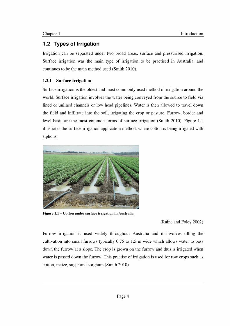
level basin are the most common forms of surface irrigation (Smith 2010). Figure 1.1
illustrates the surface irrigation application method, where cotton is being irrigated with
siphons.
Figure 1.1 – Cotton under surface irrigation in Australia
(Raine and Foley 2002)
Furrow irrigation is used widely throughout Australia and it involves tilling the
cultivation into small furrows typically 0.75 to 1.5 m wide which allows water to pass
down the furrow at a slope. The crop is grown on the furrow and thus is irrigated when
water is passed down the furrow. This practise of irrigation is used for row crops such as
cotton, maize, sugar and sorghum (Smith 2010).
Chapter 1 Introduction
Page 5
Border irrigation is similar to furrow irrigation in that it allows flow in at the top of the
field and it passes down the slope of the field to water the crop. The main difference
however between border and furrow irrigation is that border irrigation has strips
subdivided throughout the field. Typically these can be 10 to 100 m wide and range
from 200 to 1000 m long down the field. There are no distinctive furrows in the stirps or
bays, but small earthen banks. This method of irrigation is used most commonly to
irrigate pastures. While border or bay irrigation is used extensively throughout Australia
much of it is concentrated to the areas of southern New South Wales and Victoria
(Smith 2010).
The third method of surface irrigation is known as level basin irrigation. Again this
method is similar to border irrigation except there is no longitudinal slope down the
length of the field and the lengths may be shorter. This method has been widely adapted
in the United States of America; however it is not broadly practised in Australia (Smith
2010).
1.2.2 Pressurised Irrigation
Pressurised irrigation involves the use of energy to move and apply water in-field. The
water is under pressure and delivered to the field by droplets. There are many different
types of pressurised irrigation application methods which distribute the water in-field.
Depending on the crop, soil, topography, production type and many other parameters
will depend on the most effective pressurised irrigation application method (James
1988). These systems can be portable or fixed; large systems or small. Since the mid19th
century, pressurised irrigation has developed and evolved over the years. Today where
we have reliable, automated, but most importantly efficient and uniform pressurised
irrigation systems
Portable and fixed sprinkler systems cover a wide range of irrigation systems across
different agricultural and horticultural industries. However the main basic theory is
applied to all systems. Water is pressurised to a series of pipes where emitters or
sprinklers are fitted. Depending on the system layout and function will depend on how
the water is discharged from the system to irrigate the crop. Considering a system of

Chapter 1 Introduction
Page 6
portable shift irrigation pipes, sprinklers are attached by riser pipes to a main pipe and
arranged in a pattern throughout the field, coupled together via an easy insert on each
pipe. When the system is operating, the sprinklers, usually the knock impact type travel
around a full arc shooting out a velocity of water. These systems are usually used for
horticultural crops where the area of irrigation is small. A fixed pressurised system
covers a wide range of irrigation systems. Drip irrigation, microspray and handshift
irrigation are examples of this. When in operation these systems do not move, there are
fixed (James 1988). Figure 1.2 shows an example of fixed pressurised irrigation in the
form of drip irrigation. Where small drip tape is fitted underneath the trees of grape
vines and when the system is in operation water will be emitted at a controlled discharge
to the crop.
Figure 1.2 – Drip irrigation fixed under grape vines
(Irrigation 2011)
Mobile irrigation machines are different to fixed pressurised machines, as they move
when in operation. Typically these machines irrigate smaller areas then fixed sprinkler
systems, and once they have irrigated an area need to be shifted to a new area to begin
operation. An example of this is the travelling gun irrigation machine.
A travelling gun irrigator is essentially a big gun irrigator mounted on a heavy duty
chassis which moves across a field. The travel gun irrigators a sector angle as it moves
irrigates when in operation. The irrigator is usually fed from a flexible hose which is
Chapter 1 Introduction
Page 7
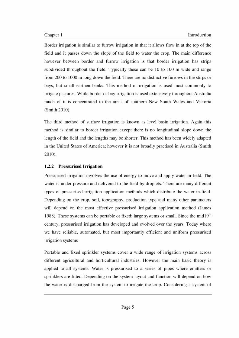
dragged behind the chassis and connected into a mains pipeline on the farm. These
machines are characteristic of operating at high pressures around 500 kPa and can water
a radius of up to 50 m. Travelling gun irrigators are widely used across eastern
Australia, particularly in the dairy, sugar and horticultural industries (Big Gun
Sprinklers n.d.).
Figure 1.3 – Cable tow travelling gun irrigator fed by flexible soft hose
(Irrigation Equipment 2011)
Figure 1.3 shows a cable tow travelling gun irrigation fed by a flexible soft hose which
is shown irrigating a pasture crop.
1.2.3 Large Mobile Irrigation Machines
Large mobile irrigation machines (LMIM’s) refer to irrigation machines which are
pressurised systems and cover broad-acre areas. LMIM’s are different to mobile
irrigation machines purely by the area which these machines are able to cover and not be
needed to be shifted such as the travelling gun irrigator. More commonly these machines
are referred to as Centre Pivots (CP) and Lateral Moves (LM). These two types of
machines are similar in that they are characteristic in operating at high flow rates and at
low pressures. The fundamentally difference between the two machines is the way in

Chapter 1 Introduction
Page 8
which they travel in the field. As the name suggests a CP is fixed on one end and the
machine pivots around this point irrigating the radius of the field at one time. A LM is
not fixed and allowed to move the width of the field and travels down the length of the
field in a linear fashion (James 1988). Figure 1.4 shows a 1250 metre lateral move
irrigation machine in a field in New South Wales.
Figure 1.4 – A 1250 metre Lateral Move in New South Wales
(Center Irrigation 2010)
1.2.4 Background to Large Mobile Irrigation Machines
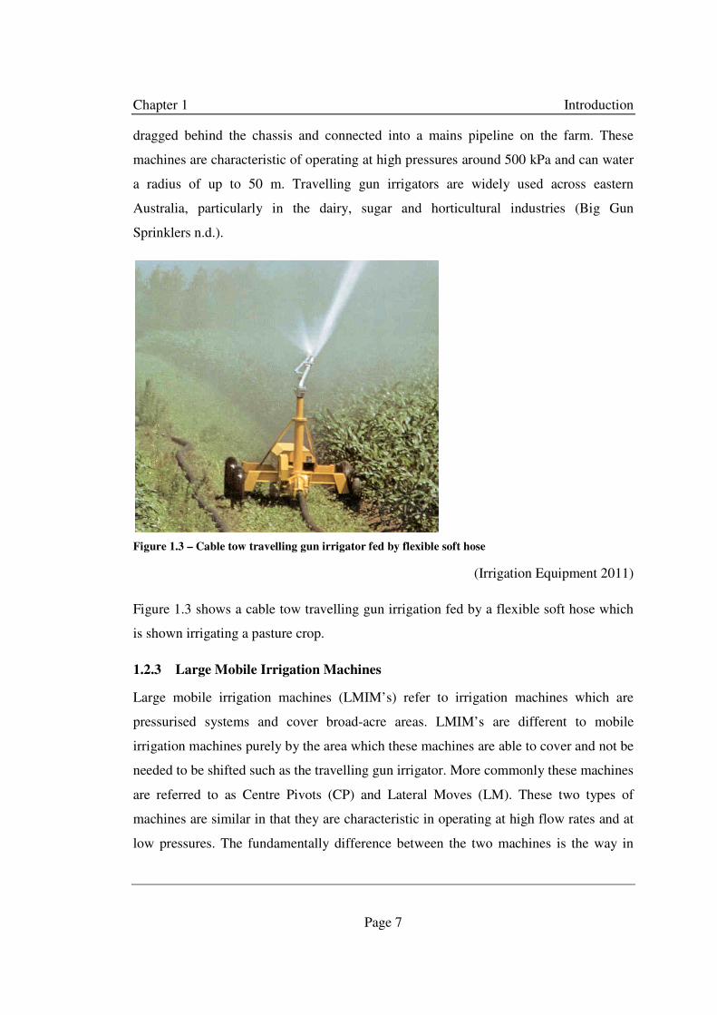
Large mobile irrigation machines were first developed in the 1940’s in Nebraska, USA
where Frank Zybach designed and built the first prototype. This machine involved the
placement of impact sprinklers on a long steel pipe, which moved around the field in a
circle. The system was shifted around the field by water pressure. Figure 1.5 shows
Zybach’s first design (Mander & Hays 2010).
Chapter 1 Introduction
Page 9
Figure 1.5- The first large mobile irrigation machine
Over the years Zybach and his business partners modified the original prototype, raising
the lateral line higher to allow for irrigation of tall crops such as maize. The other
significant change was the sprinkler system; impact sprinklers require a lot of pressure
to operate correctly, which in turn raised the energy requirements for the machine.
During the energy crisis in the 1970’s a new water distribution system was required to
lower running costs of the machine; this introduced low-pressure static plate sprinklers.
These sprinklers were located in droppers under the main lateral line along the length of
the machine (Foley & Raine 2001).
Valley, now known as Valmont Industries was the pioneer company, directed by Robert
Daugherty, which first manufactured commercial large mobile irrigation machines.
Since then more than 60 manufacturing companies realized the potential of these
machines and so started manufacturing; today the manufacturing of all LMIM’s in the
world lies with a handful of companies. Among these are the four main manufacturing
companies which have dominated the world market. These are, Lindsey Zimmatic,
T&L, Valley and Reinke, all four companies have their company headquarters in
Nebraska, USA (Foley & Raine 2001).

Chapter 1 Introduction
Page 10
It has been said that the development of centre pivot irrigation has been the most
important advance in agricultural technology since the replacement of tractors over the
horse-drawn power. Since the invention of the LMIM’s, the area under irrigation in the
US as dramatically increased. Approximately 32% of all irrigation within the US is
under LMIM. Australia was first introduced to LMIM’s in the 1960’s. South Australia
and Victoria were the first states to adopt the technology with interest. In 2008-09
Australia’s irrigation industry had about 15% under LMIM’s (Australian Bureau of
Statistics 2010).
1.2.5 Function of Large Mobile Irrigation Machines
Water is fed into the machine under pressure and travels the length of the machine via
the main lateral pipeline. This lateral pipeline is supported by a series of towers which
are spaced at 24 to 76 metres (James 1988). The length of this lateral pipeline will
depend in its system type. In Australia, centre pivots are usually about 500 metres in
length, commonly though they are around 400 metres long, which irrigates an area of
50.3 hectares. Lateral moves are not commonly used overseas. However their popularity
in the Australia cotton industry has seen lateral moves being installed with a lateral
pipeline of 1000 metres (Foley & Raine 2001). The main lateral pipeline can be
manufactured of different materials depending on the individual’s water quality these
include, aluminium, stainless steel, chromium and nickel and galvanised steel. While the
spans pipe size will vary with the manufacturer the most common internal diameters of
the main lateral pipeline spans range from 135 to 247.8 mm with the most common sizes
being 162, 197 and 213 mm, the typically pipe wall thickness of the span is 2.77 mm
(Foley & Raine 2001).
The towers which support this main lateral pipeline above the crop canopy are powered
either by hydraulic or electric motors. Gearboxes and drive wheels and shafts are also
fitted onto each tower. For a centre pivot the rotational speed of the machine is
controlled by the outermost tower and every other tower is moved with reference to this
tower. A lateral move will travel at the same speed as it moves in a linear fashion down
the length of the field. The water supply into a lateral move will typically be located

Chapter 1 Introduction
Page 11
either in the middle or one end via a cart-tower assembly which will typically also carry
a mobile power plant.
From the main lateral pipeline of the centre pivot or lateral move hydraulic couplings
are used to make a delivery point. Goosenecks are usually used which are installed into
the top of the main lateral pipeline 19 mm plastic droppers are fitted into these either
over boombacks or straight down to deliver the water to the sprinkler application
package.
The sprinkler application package (SAP) is the most important component of the
machine, as it is effectively is carrying this package over the crop. The SAP consists of a
pressure regulator, nozzle and plate. This is a sprinkler type application type, low energy
precision application (LEPA) systems are become more common as they direct the
water into the furrow of the crop, without the traditional droplet method with sprinklers.
There are two main manufacturers who produced the application packages, either
sprinkler or LEPA, and these are fitted on the four manufacturers of the LMIM’s. In
2001 it was reported that 58% of growers surveyed used pressure regulators with their
LMIM’s application packages (Foley and Raine 2001). 10 years later it is estimated that
90% of machines commissioned have pressure regulators installed with their application
packages.
A pressure regulator which is located just upstream of the application package outputs a
constant pressure, despite different input pressures into the pressure regulator along the
length of the main lateral pipeline. This different input pressure may be due to
topography changes along the length of the machine as it operates infield, differing input
pressure due to changes of the pressure of the supply, such as a drawdown profile in a
bore and fluctuations of the pump. However no matter what the changes of the input
pressure the pressure regulator is reported to give a set constant output pressure.
1.3 Irrigation Performance
The performance of an irrigation system can have a different importance to different
irrigators, depending on their operation and irrigation type. In describing the

Chapter 1 Introduction
Page 12
performance, a number of measures are taking into consideration. These measures are
the application efficiency, requirement efficiency and various uniformity efficiencies.
The application efficiency is give below as equation 1.1
�� �%� = ��� ��� � � �� ������ ��� ��� � �� � � � �� �
1.1
The water lost to canopy interception, evaporation and spray drift in pressurised
irrigation, tailwater runoff and deep percolation in surface irrigation can be evaluated
through the application efficiency (Smith 2010).
The requirement efficiency is a measure of how well the irrigation has brought the soil
moisture store back up the required level. Equation 1.2 gives the equation to calculate
the requirement efficiency (Smith 2010).
�� �%� = ��� ��� � � �� ������ ��� ��� � ���� � � � ��� � � �� ������ ���
1.2
The third measure of discussion of irrigation performance is uniformity. Spatial
variability will be present through different applied depths over the irrigated (surface or
pressurised) field if one of the more is present:
• For surface irrigation, variations in applied depth along the furrow or bay as a
result of the surface hydraulics/soil infiltration interaction.
• Variations in performance between furrows due to differences in the inflow rate,
the infiltration characteristic or other hydraulic properties.
• Variations in applied depth in sprinkler irrigation due to the sprinkler pattern,
sprinkler spacing (overlap) or lane spacing in the case of travelling irrigators.
• Effect of wind on the sprinkler pattern.
• Variations in the nozzle or emitter outflows along the length of any sprinkler or
trickle irrigation pipeline.
• The stop-start pattern of movement of “continuously” moving systems, such as
centre pivot or lateral move machines.

Chapter 1 Introduction
Page 13
• For mobile systems (centre pivots and lateral moves) variations in the land
surface and hence pipeline elevation.
• Variations in emitter or pressure regulator performance due to size or other
variations occurring during manufacture of drip irrigation components.
• Other causes such as temperature variations, wear and blockage of emitters, and
fluctuations in pump performance.
(Smith 2010)
The above list shows the importance of correct design and management in order to get
the best out of the irrigation system whatever the system type may be. The Christiansen
Uniformity Coefficient which is given by equation 1.3 below is the mostly widely used
uniformity measure for sprinkler irrigation.
��� = 100 �1 − �����
� = ∑��" − �����#
1.3
where m is the absolute deviation of the applied depth, xbar is the mean applied depth
and n is the number of depth measurements.
Another uniformity measure is the Uniformity Coefficient (UC) which is given by
equation 1.4
�� = 100[1 − 0.8 � '���� ] 1.4
where σ is the standard deviation of the applied depths. If the applied depths are
normally distributed then CUC and UC are equal.
Distribution uniformity is used across both surface and pressurised irrigation, however it
is most popular with surface irrigation.
Chapter 1 Introduction
Page 14
)��%� = * �# � + �� 25% � �..� � � .�ℎ�* �# �..� � � .�ℎ�
1.5
The last uniformity measure is called the emission uniformity which is given below as
equation 1.6.
�� �%� = 100�1 − 1.27 ��1# � �2"1
���� 1.6
where: CVn is the coefficient of variation of the individual emitters due to
manufacturing differences, n is the number of emitters per plant, qmin is the discharge for
an average emitter at minimum pressure and qbar is the average of design discharge for
the emitters. The emission uniformity was developed for drip and trickle irrigation.
The effect of non-uniform irrigation can result in substantial changes in the yield of the
crop being irrigated due to spatial variation. Along with this with the application and
requirement efficiencies will evaluate the overall performance of the farms irrigation
systems and this can give the irrigator a benchmark to improve their operations on farm.
1.4 Broad Aim
This project aims to accurately characterise the hydraulic performance of pressure
regulators used on large mobile irrigation machines by developing a testing
methodology.
1.5 Objectives
The main objectives of this work are to:
1) Review the test methodologies from formal literature in this area of study and to
develop an understanding of the manufacture literature regarding these pressure
regulator devices.
2) Design and develop a testing methodology to accurately determine the
performance of pressure regulators.

Chapter 1 Introduction
Page 15
3) Calculate the sample size and develop and evaluate the testing procedure which
adequately characterises manufacturer’s variation in pressure regulator
manufacture.
4) Analyse gathered data sets and present performance of pressure regulators and
their variation based on the developed testing methodologies.
5) Bed the initial work for the development of a mathematical model which
accurately describes the hydraulic performance of the pressure regulators used in
broad-acre irrigation.
1.6 Structure of this Dissertation
This chapter has provided a brief background to the subject area and has introduced the
objectives of the remaining six chapters of this dissertation. Chapter two provides a
formal literature review of this area of study and a summary of their finding. The
literature review covers previous studies to understand pressure regulator performance
and provides details of the manufacturers of pressure regulators and introduces their
products. Chapter two also discusses basic theories behind pressurised hydraulic
measurement and the introduction of statistical procedures which will be used in later
chapters. Chapter three deals with the methodology taken with each testing stage and
how the testing rig was used to obtain the results and also discusses the process of
calibration of the sensors used in the testing rig. Chapter three also breaks the pressure
regulator down into each individual components and explains the interactions each part
has with each other and how they work together to perform its function.
Chapter four reports the results obtained in each testing stage. Chapter five provides a
detailed discussion on the results presented in chapter four and their outcomes back to
the industry. This chapter also compares the results from chapter four to the results from
the formal literature. Chapter six outlines the key findings of this research and states the
conclusions made on this study. Chapter seven outline recommendations made with
reference to chapters five and six for further research needed in this area.

Chapter 2 Literature Review
Page 16
Chapter 2 LITERATURE REVIEW
2.1 Introduction
This chapter introduces the reader to current and past literature on the topic of
discussion and also establishes basic concepts which are used widely in later chapters
which describe the processes in undertaking different tests.
2.2 Flow Measurement
In any hydraulic setup, whether it is a pipe or open channel the measurement or
evaluation of the discharge of the system is crucial. Many design parameters and
calculations need an accurate value for the systems discharge. The discharge of a system
is made up of two components, velocity of the fluid and the area of which the fluid is
flowing. The flow entry into a system will equal the flow exiting the system. This is
described by the Continuity equation, shown by equation 2.1.
3 = ��
�4�4 = �5�5
2.1
where Q = Flow rate (m3/s), A = Cross sectional area (m2) and V = Velocity (m/s)
Depending the desired accuracy and system type will depend on the type of flow
measurement used.
2.2.1 Flow measurement through pipes
It is through the use of the energy, continuity and momentum equations, where simple
methods can be applied to measure the flow in hydraulic situations.
Following the law of the conservation of energy, energy cannot be created or destroyed.
This provides the basis of Bernoulli’s energy equation given below

Chapter 2 Literature Review
Page 17
.467 + �4
5
27 + 94 = .567 + �5
5
27 + 95 − ℎ: − ℎ2 + ℎ; 2.2
where p = Pressure (kPa), ρ = Density of fluid (kg/m3), g = Local gravitational
acceleration constant (m/s2), v = Velocity (m/s), z = Elevation (m), hf = Friction Loss (m
head), hm = Local Loss (m head) and hp = Addition by pump (m head)
(Moore 2009; Nalluri & Featherstone 1982)
This equation forms the bases of the principle of how to calculate the flow within a
venturi metre. With a venturi the pressure difference is created by from a sudden
constriction in the cross sectional profile of the pipeline. From equation 2.2 when the
fluid enters the smaller diameter pipe the velocity will increase. From the increase in
velocity the pressure will decrease to compensate for the gain of energy in terms of
velocity. It is through this relationship that a discharge can be derived.
A pitot tube is a simple piece of tube which is placed into the flow of a fluid, creating a
‘stagnation point’. Following the same basic principles in section 2.4.1.1 the flow can be
measured. The column of water within this tube will be higher can the height of water
being passed. The difference in height will be the energy created by the velocity of the
fluid (Nalluri & Featherstone 1982).
There are several different flow meters currently on the market, each have their own
measurement techniques. The flow meter used for this dissertation is an electromagnetic
ultrasonic type. This type of flow meter induces a voltage across a magnetic field. The
voltage across this magnetic field will be directly proportional to the velocity of the
fluid. With an accurate cross sectional are known the discharge can be calculated via
equation 2.1.

Chapter 2 Literature Review
Page 18
2.3 Pressure Measurement
Pressure is the unit of measure of force divided by area. The SI unit of pressure is the
Pascal, and follows equation below.
< = =�
2.3
where P= Pressure (Pa), F = Force (N), A = Area (m2)
There are three different meanings of pressures which need to be noted, these include
gauge, absolute and standard atmospheric pressure. The gauge pressure is an arbitrary
pressure measurement which is relative to the local atmospheric pressure. From this the
absolute pressure may be positive or negative depending on the local atmospheric
pressure. The pressure can be measured in two ways;
a) as a force per unit area (Pa)
b) as an equivalent height of column of fluid (Pa or metres head)
From the first pressure measurement, equation 2.3 is used to evaluate the pressure. The
second is evaluated by equation 2.4 below.
< = 6gh 2.4
where P = Pressure (Pa) and h = Column height of fluid (m)
Commonly within the water and hydraulic industries gauge pressure is expressed in
metres head of water. The unit of head is defined as the energy per unit weight of fluid
ℎ = <67
2.5
(Chadwick, Morfett & Borthwick 1986; Nalluri & Featherstone 1982)
2.3.1 Pressure measurement through pipes

Chapter 2 Literature Review
Page 19
Bourdon Gauges
In almost all fluid pressurised systems, gauges would be used to monitor and measure
the pressure in the pipeline or pressurised system. A gauge is a device which is fitted to
a system usually by a threaded fitting. Fluid from the system is allowed to enter into the
gauge via a small opening; the fluid fills a hollow metallic tube called at bourdon tube.
When the pressure is raised this tube flexes and it is this flex movement which is
transferred to a dial and a pressure reading can be read off the gauge (Factory Direct
Pipeline Products 2011). There are many different types and qualities of gauges,
depending on the application and accuracy required.
Electronic Pressure Transducers
A pressure transducer is another method is measure the pressure within a system. When
calibrated and set-up correctly pressure transducers have the ability to give high
accuracy and repeatability and transfer back the information to an automotive or
electronic data collection system. A pressure transducer is effectively a strain gauge.
The device is tapped into a system the same as a gauge and when the pressure in the
fluid is raised a small diaphragm is displaced. This movement is measured and sent as a
signal voltage to be read via some acquisition method (Beliveau 2011). As with pressure
gauges, there are many different types of pressure transducers giving different degrees
of accuracy in their function. Manufactures of Pressure Regulators
There are a number of pressure regulator manufactures currently in operation. Nelson
Irrigation Co and Senninger Irrigation Inc are the two main manufactures of pressure
regulation devices for Large Mobile Irrigation Machines. As well as these companies
there are a number of smaller manufactures which deliver for other agricultural and
horticultural industries.

Chapter 2 Literature Review
Page 20
2.4 Pressure Regulators Manufacturers
2.4.1 Nelson
Nelson Irrigation Co is a global sprinkler and irrigation manufacturing company. There
headquarters are based in Walla Walla, Washington, United States of America. The
company is a major supplier of many different sprinkler and fittings used on Large
Mobile Irrigation Machines and is many other fixed sprinkler systems.
Nelson Irrigation Co manufactures two different models of pressure regulators, a
UNIVERSAL-FLO regulator and a HI-FLO regulator.
The model of Nelson pressure regulators is the main product used on Large Mobile
Irrigation Machines. The UNIVERSAL-FLO pressure regulator come in a range of
different set pressures, these are, 6, 10, 15, 20, 25, 30, 40 and 50 PSI. There are four
different types of connection types available with this model of regulator, depending on
the intended application method. These are, the pipe thread connection, ¾” FNPT x ¾”
FNPT, the 3000 series pivot connection, ¾” FNPT x 3000 ST, the hose thread
connection, ¾” FHT x ¾” MHT, barbed 3000 series pivot connection, ¾” male barb x
3000 ST. The most common pressure regulator used on centre pivots and lateral moves
in Australia is the ¾” male barb x 3000 ST, 10 PSI pressure setting. The flow setting for
this model ranges from 0.0305 – 0.5055 L/s for the 6 Psi pressure setting and 0.0305 –
0.7555 L/s for the other outlet set pressures (Pressure Regulation, n.d.).
The Nelson HI-FLO pressure regulator model is similar to the UNIVERSAL-FLO
model, however just as the name suggest this model allows for a greater discharge
through the device. This is done by increase the area of the tube through the device.
2.4.2 Senninger
Senninger Irrigation Inc was established in 1963 and continues to be a world leader in
the manufacturing and supplier of irrigation sprinkler packages and fittings to irrigation
over many industries across the world. The company’s headquarters are located in
Clermont, Florida, United States of America. Senninger manufacture eight different
models of pressure regulators these include, Pressure Regulator Landscape Grade
Chapter 2 Literature Review
Page 21
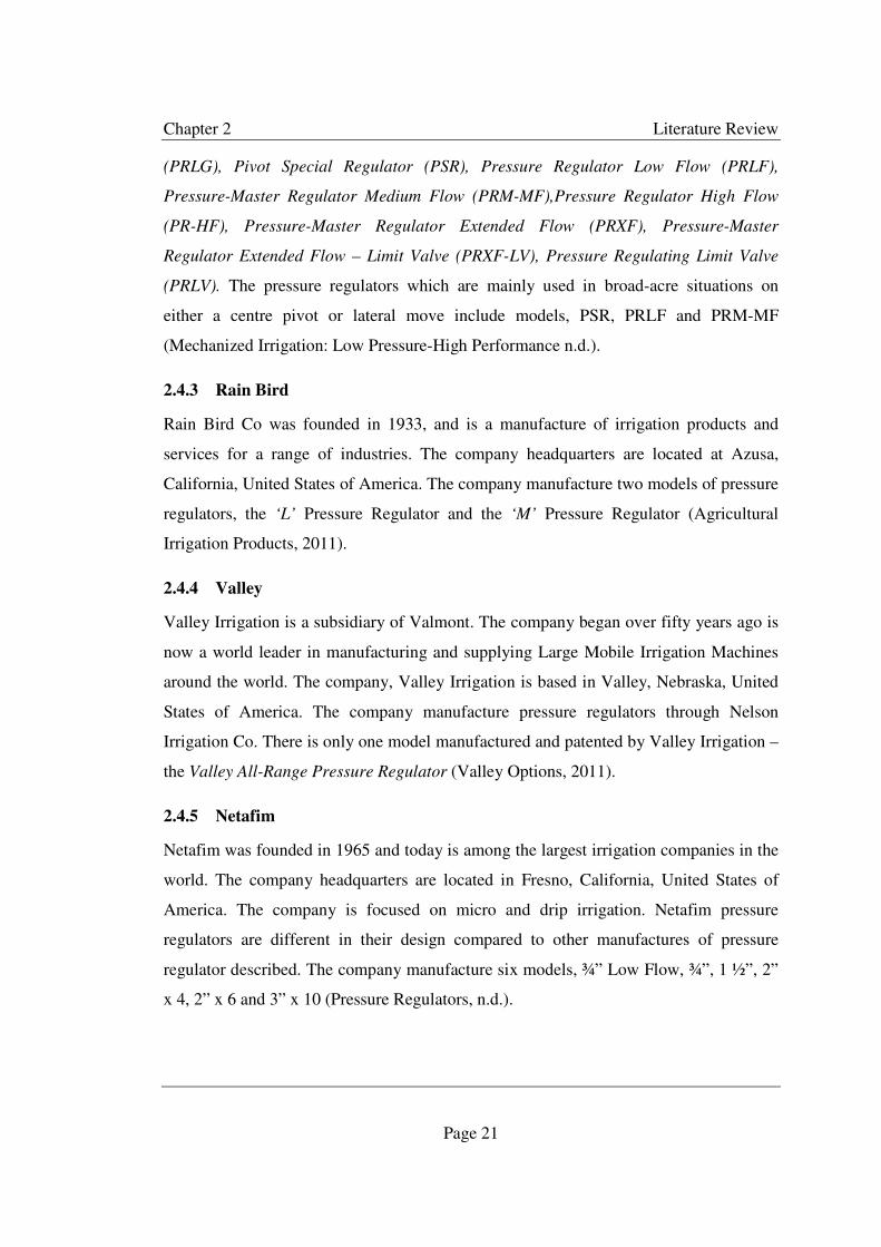
(PRLG), Pivot Special Regulator (PSR), Pressure Regulator Low Flow (PRLF),
Pressure-Master Regulator Medium Flow (PRM-MF),Pressure Regulator High Flow
(PR-HF), Pressure-Master Regulator Extended Flow (PRXF), Pressure-Master
Regulator Extended Flow – Limit Valve (PRXF-LV), Pressure Regulating Limit Valve
(PRLV). The pressure regulators which are mainly used in broad-acre situations on
either a centre pivot or lateral move include models, PSR, PRLF and PRM-MF
(Mechanized Irrigation: Low Pressure-High Performance n.d.).
2.4.3 Rain Bird
Rain Bird Co was founded in 1933, and is a manufacture of irrigation products and
services for a range of industries. The company headquarters are located at Azusa,
California, United States of America. The company manufacture two models of pressure
regulators, the ‘L’ Pressure Regulator and the ‘M’ Pressure Regulator (Agricultural
Irrigation Products, 2011).
2.4.4 Valley
Valley Irrigation is a subsidiary of Valmont. The company began over fifty years ago is
now a world leader in manufacturing and supplying Large Mobile Irrigation Machines
around the world. The company, Valley Irrigation is based in Valley, Nebraska, United
States of America. The company manufacture pressure regulators through Nelson
Irrigation Co. There is only one model manufactured and patented by Valley Irrigation –
the Valley All-Range Pressure Regulator (Valley Options, 2011).
2.4.5 Netafim
Netafim was founded in 1965 and today is among the largest irrigation companies in the
world. The company headquarters are located in Fresno, California, United States of
America. The company is focused on micro and drip irrigation. Netafim pressure
regulators are different in their design compared to other manufactures of pressure
regulator described. The company manufacture six models, ¾” Low Flow, ¾”, 1 ½”, 2”
x 4, 2” x 6 and 3” x 10 (Pressure Regulators, n.d.).

Chapter 2 Literature Review
Page 22
2.5 Pressure Regulators and Large Mobile Irrigation Machines
This research has been set out to investigate and further understand the workings of
pressure regulators, within the irrigation industry, primarily however with the use of
large mobile irrigation machines. As described in section 2.4, they are many
manufacturers and types of pressure regulators. The most commonly used pressure
regulators on LMIM within Australia, are made by Nelson Irrigation Co and Senninger
Irrigation Inc.
On a large mobile irrigation machine a pressure regulator is installed immediately
upstream of the nozzle. There is one pressure regulator to each nozzle of the machine.
Over the length of the machine this equate to a considerable number of pressure
regulator, amounting to a significant cost. The nozzle and sprinkler package is installed
directly downstream ensuring the constant output pressure from the pressure regulator is
passed into the sprinkler and subsequently onto the crop. Figure 2.3 illustrates a typical
installation of a pressure regulator on a LMIM.
Figure 2.1 - Pressure Regulator and a LMIM

Chapter 2 Literature Review
Page 23
2.6 Previous Research
This research work is concerned about determining the performance characteristics of
pressure regulation devices used in broad-acre irrigation. As part of this Literature
Review, previous literature on the performance of these devices was researched. There
has been limited research on this field, with only a few research papers written. Most of
this research has been collated in the 1980’s when large mobile irrigation machines,
particular centre pivots had been expanding rapidly. With soaring energy costs and with
water use efficiency becoming major issues within the irrigation industry, there is a need
to review this research and continue the development and understanding of the
performance of pressure regulators.
In 1990 von Bernuth and Baird published a paper entitled ‘Characterising Pressure
Regulator Performance’. This research involved testing three popular brands of pressure
regulators, Senninger, Nelson and RainBird. This paper is a very comprehensive study
which set out to try to characterise performance of pressure regulators used in
pressurised irrigation systems. The effect from variations of pressure entering nozzles,
sprinklers or emitters within pressurised irrigation systems can lead to serious
distribution uniformity and efficiency effects.
The study began as one which tested and reported the regulators performance and
evolved to developing the testing procedure for testing and characterizing the
performance of regulators. It was found from this study that the variation not only
between pressure regulators but also between test repeats was greater than expected.
Due to this, the methodology is critical in the characterisation of the devices.
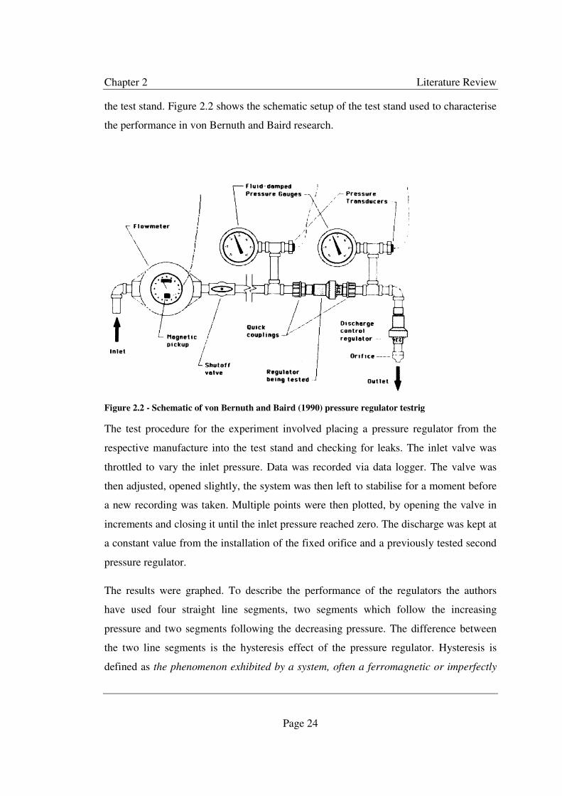
A test stand was developed for testing. The rig incorporated an analogue calibrated
magnetic pickup flowmeter upstream of a shutoff valve. A regulator was placed
downstream of this between two quick couplings used for convenient placement into
and out of the test stand. Fluid-damped pressure gauges and pressure transducers was
used, either side of the quick couplings for inlet and outlet pressure measurement of the
pressure regulator. To control the discharge a previously tested regulator was used and
installed immediately upstream of a precision orifice from which the fluid exited from
Chapter 2 Literature Review
Page 24
the test stand. Figure 2.2 shows the schematic setup of the test stand used to characterise
the performance in von Bernuth and Baird research.
Figure 2.2 - Schematic of von Bernuth and Baird (1990) pressure regulator testrig
The test procedure for the experiment involved placing a pressure regulator from the
respective manufacture into the test stand and checking for leaks. The inlet valve was
throttled to vary the inlet pressure. Data was recorded via data logger. The valve was
then adjusted, opened slightly, the system was then left to stabilise for a moment before
a new recording was taken. Multiple points were then plotted, by opening the valve in
increments and closing it until the inlet pressure reached zero. The discharge was kept at
a constant value from the installation of the fixed orifice and a previously tested second
pressure regulator.
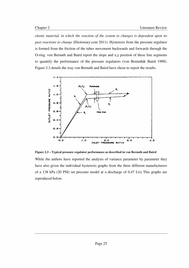
The results were graphed. To describe the performance of the regulators the authors
have used four straight line segments, two segments which follow the increasing
pressure and two segments following the decreasing pressure. The difference between
the two line segments is the hysteresis effect of the pressure regulator. Hysteresis is
defined as the phenomenon exhibited by a system, often a ferromagnetic or imperfectly
Chapter 2 Literature Review
Page 25
elastic material, in which the reaction of the system to changes is dependent upon its
past reactions to change (Dictionary.com 2011). Hysteresis from the pressure regulator
is formed from the friction of the tubes movement backwards and forwards through the
O-ring. von Bernuth and Baird report the slope and x,y position of these line segments
to quantify the performance of the pressure regulators (von Bernuth& Baird 1990).
Figure 2.3 details the way von Bernuth and Baird have chose to report the results.
Figure 2.3 – Typical pressure regulator performance as described in von Bernuth and Baird
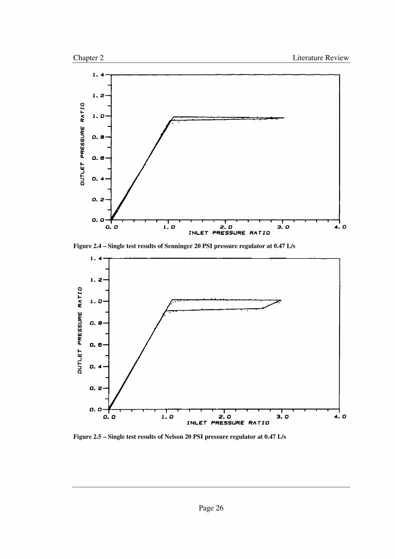
While the authors have reported the analysis of variance parameter by parameter they
have also given the individual hysteresis graphs from the three different manufacturers
of a 138 kPa (20 PSI) set pressure model at a discharge of 0.47 L/s) This graphs are
reproduced below.
Chapter 2 Literature Review
Page 26
Figure 2.4 – Single test results of Senninger 20 PSI pressure regulator at 0.47 L/s
Figure 2.5 – Single test results of Nelson 20 PSI pressure regulator at 0.47 L/s

Chapter 2 Literature Review
Page 27
Figure 2.6 – Single test results of Rainbird 20 PSI pressure regulator at 0.47 L/s
Kincaid et al also reports the pressure regulators hysteresis effect as the performance
characterisation. This study was sponsored by an agency of the United States
Government and the purpose of the study was to evaluate the characteristics of irrigation
components and to evaluate the economics of very low pressure irrigation devices used
on centre pivot irrigation systems. This was a twofold study one side involved as
investigation into the characteristics of pressure regulators and the other side was to
evaluate low pressure devices application methods used in pressurised irrigation. The
two methods investigated were spray nozzles and furrow drops (bubblers). Reservoir
tillage was also evaluated with the use of low pressure devices on centre pivot and
lateral move irrigation to see the effect and if it improved the irrigation. This literature
review will only concentrate on the first stage of the study the characterisation of
pressure regulators.
This study tested pressure regulators in a laboratory setting from two different
manufactures, Nelson and Senninger. The purpose of the study was to evaluate the
pressure regulation accuracy compared to the stated nominal output pressures. Five
devices from each pressure set were tested and the results averaged. For the Nelson

Chapter 2 Literature Review
Page 28
regulators, devices with pressure sets of 10, 15 and 20 psi were tested, and for Senninger
regulators, 6, 10, 15 and 20 psi nominal pressure were tested. The experiment tested
three different discharges, 0.252, 0.504 and 0.756 L/s (4, 8 and 12 US gpm). The
different discharges were obtained by using different sized nozzles. The pressures both
input and output were measured using calibrated pressure gauges.
The authors wanted to simulate the condition experienced to the pressure regulator as it
is in the field on a LMIM. As the machine travels uphill the inlet pressure to the pressure
regulator is decreasing, similarly as the machines travels downhill the inlet pressure is
increasing. To simulate this effect on the lab bench, the outlet pressure was measured as
the inlet pressure was increased from the pressure regulators nominal set pressure up to
551.58 kPa (80 PSI) at 68.94 kPa (10 PSI) increments. Once this limit was reached the
pressure was then decreased back to the starting point. The same nozzle size was used
for each test.
The results of this experiment show the hysteresis curve for different models of each
manufacturer at a medium discharge of 0.504 L/s (8 US gpm).
Chapter 2 Literature Review
Page 29
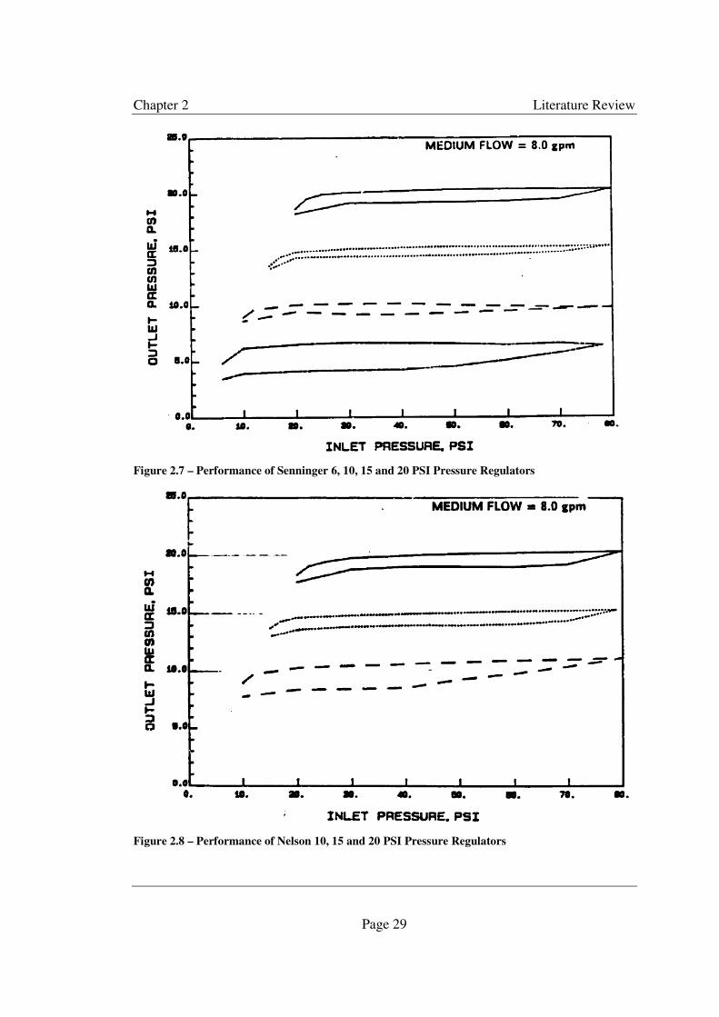
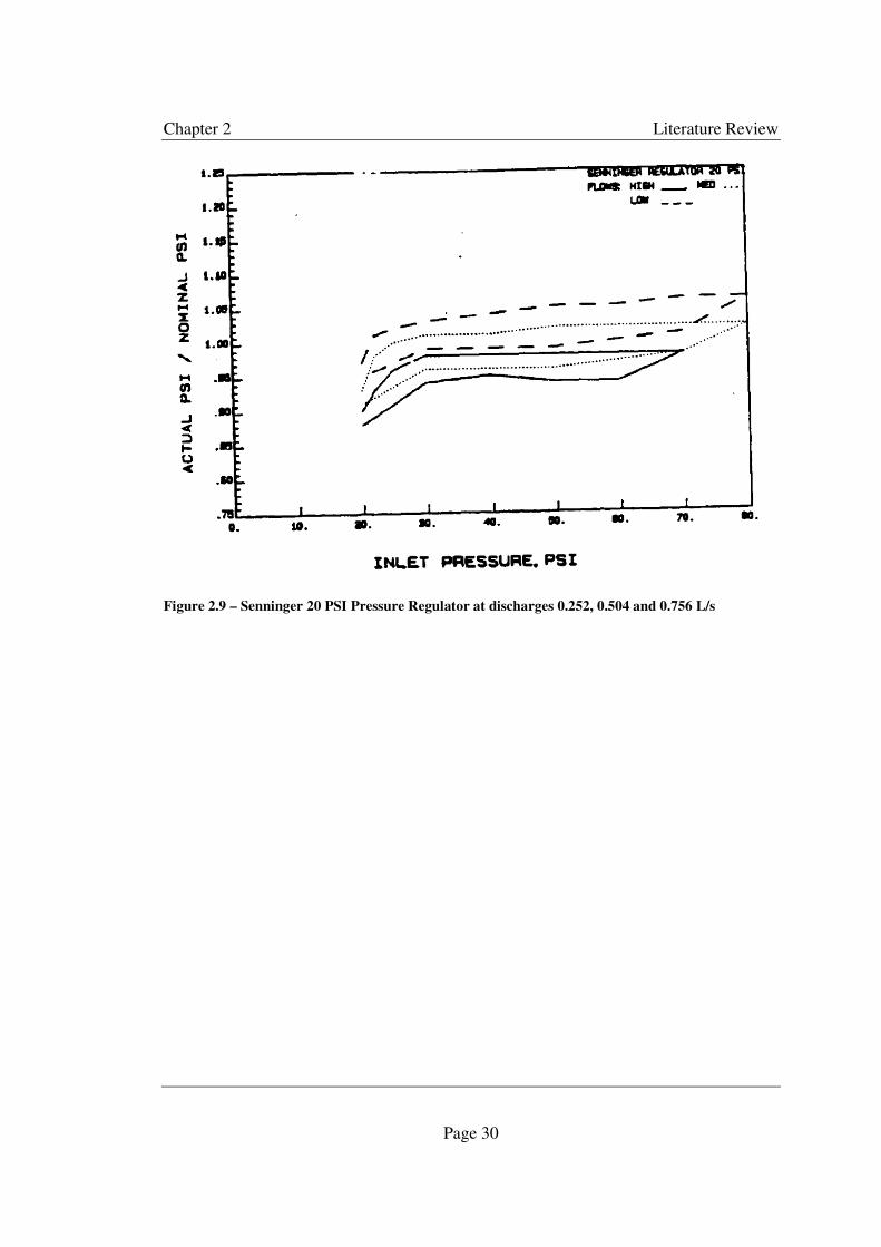
Figure 2.7 – Performance of Senninger 6, 10, 15 and 20 PSI Pressure Regulators
Figure 2.8 – Performance of Nelson 10, 15 and 20 PSI Pressure Regulators
Chapter 2 Literature Review
Page 30
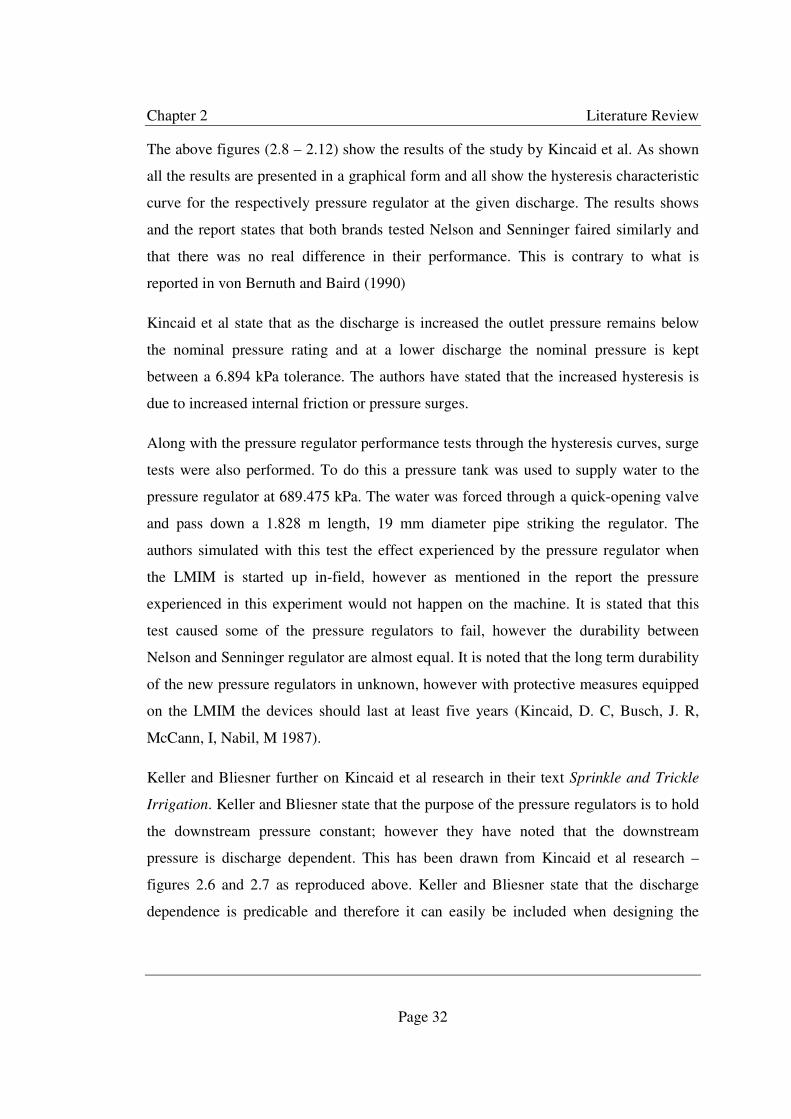
Figure 2.9 – Senninger 20 PSI Pressure Regulator at discharges 0.252, 0.504 and 0.756 L/s

Chapter 2 Literature Review
Page 31
Figure 2.10 – Senninger 15 PSI Pressure Regulator at discharges 0.252, 0.504 and 0.756 L/s
Figure 2.11 – Senninger 10 PSI Pressure Regulator at discharges 0.252, 0.504 and 0.756 L/s
Chapter 2 Literature Review
Page 32
The above figures (2.8 – 2.12) show the results of the study by Kincaid et al. As shown
all the results are presented in a graphical form and all show the hysteresis characteristic
curve for the respectively pressure regulator at the given discharge. The results shows
and the report states that both brands tested Nelson and Senninger faired similarly and
that there was no real difference in their performance. This is contrary to what is
reported in von Bernuth and Baird (1990)
Kincaid et al state that as the discharge is increased the outlet pressure remains below
the nominal pressure rating and at a lower discharge the nominal pressure is kept
between a 6.894 kPa tolerance. The authors have stated that the increased hysteresis is
due to increased internal friction or pressure surges.
Along with the pressure regulator performance tests through the hysteresis curves, surge
tests were also performed. To do this a pressure tank was used to supply water to the
pressure regulator at 689.475 kPa. The water was forced through a quick-opening valve
and pass down a 1.828 m length, 19 mm diameter pipe striking the regulator. The
authors simulated with this test the effect experienced by the pressure regulator when
the LMIM is started up in-field, however as mentioned in the report the pressure
experienced in this experiment would not happen on the machine. It is stated that this
test caused some of the pressure regulators to fail, however the durability between
Nelson and Senninger regulator are almost equal. It is noted that the long term durability
of the new pressure regulators in unknown, however with protective measures equipped
on the LMIM the devices should last at least five years (Kincaid, D. C, Busch, J. R,
McCann, I, Nabil, M 1987).
Keller and Bliesner further on Kincaid et al research in their text Sprinkle and Trickle
Irrigation. Keller and Bliesner state that the purpose of the pressure regulators is to hold
the downstream pressure constant; however they have noted that the downstream
pressure is discharge dependent. This has been drawn from Kincaid et al research –
figures 2.6 and 2.7 as reproduced above. Keller and Bliesner state that the discharge
dependence is predicable and therefore it can easily be included when designing the

Chapter 2 Literature Review
Page 33
sprinkler, nozzle and pressure regulator package, however the authors have not
described this process in detail.
Keller and Bliesner take a difference approach to describe how the hysteresis curves
perform. Caused by mechanical friction within the devices, Keller and Bliesner explain
that when the inlet pressure is rising the discharge (outlet) pressure follows the lower leg
on the hysteresis curve, conversely when it is falling it follows the upper leg. The
explanation is different to von Bernuth and Baird journal paper which is opposite to
what is explain in Keller and Bliesner. Keller and Bliesner say that the average deviation
of the outlet pressure due to varying inlet pressure is about 7 kPa (1 PSI), which for a 10
PSI set pressure regulator is a 10% variation.
In the three literature pieces detailed above, all have explained the importance of
maintaining a 20.684 – 34.473 kPa (3-5 PSI) increase above the nominal set pressure of
the pressure regulator. Keller and Bliesner have incorporated the discharge dependency
through the following equation.
<@ = <;A − �<BC�@ = <;A − D��@E��5 2.6
where Pj = Available sprinkler operating pressure at radius rj (kPa), Ppr = Average outlet
pressure (which is usually the nomial pressure rating of the pressure regulator at low
discharge (kPa), (Pcv) j= Minimum pressure loss across the regulator for qj at the radius r
j, (kPa), qj = Desired outlet discharge at radius rj (L/s), cv = Flow coefficient that is
numerically equal to the discharge when (Pcv)j = 1 kPa and K = Appropriate unit
pressure loss for the specific measurement units used (1 kPa).
Keller and Bliesner report that the ‘better' pressure regulators available for use in centre-
pivots and lateral moves have a high flow coefficient. For a unit pressure loss of 1 kPa
the cv value is approximately 0.24 L/s (unit pressure loss of 1 PSI, cv ~ 10 US GPM). It
is noted the flow coefficient values are usually the same for pressure regulators with the
same casing shape and configuration regardless of the devices set pressure rating. Keller
and Bliesner also report that the weighted average coefficient of discharge variation for
a pressure regulator with a fixed nozzle combination follows the equation,

Chapter 2 Literature Review
Page 34
�F ≈ 1 − �1 − 0.97�4/5 ≈ 0.015 2.7
(Keller, J & Bliesner, R.D 1990)

Chapter 2 Literature Review
Page 35
2.7 Statistical Analysis
2.7.1 Introduction
In our modern world of mechanical and automated control of manufacturing engineering
within factories, statistical variation has become an important factor of control. No two
products produced on the factory floor will perform or behaviour in exactly the same
way. However there needs to be tolerance boundaries put in place to maintain high
degrees of control over the products variation. Depending on the product being
manufactured and its intended use will influence the tolerance boundaries on the
products manufacture. An example of this would be filling bottles of water. Down the
factory line, bottles are placed on a conveyer belt and fed down the production line. No
two bottles filled by the automation production process will be exactly the same volume.
It is due to this reason the production line would need to be calibrated to a particular
tolerances, depending on the accuracy and precision of the volume needed.
Pressure regulators are no different to filling bottles with water to a nominal volume. A
Nelson 10 PSI Uni-Flo pressure regulator is made up of nine different individual
components, a spring, two different sized O-rings, a tube and incorporated skirt seal, an
internal casing, a redistribution plug, two parts of the external casing and six phillips
head screws. Each of these components are made and assembled on the factory floor and
each with their own individual tolerance limits. When all the components are assembled
into their respective position these nine components make up the pressure regulator. The
manufacturer states that the 10 PSI pressure regulator will maintain a constant output
pressure no matter of the input pressure. This 10 PSI pressure rating however is a
nominal value and will change from device to device. To understand this variation an
important question is how many devices need to be tested or evaluated to know the
manufacturing variability of the pressure regulators.
There are many different models of pressure regulator, all which have been described in
section 2.7.1. From this it can be seen the vast number of makes and models of pressure
regulators on the market. Furthermore in trying to quantify the pressure regulators
manufacturing variability the test procedure to do this needs to be repeatable and expose

Chapter 2 Literature Review
Page 36
each device to exactly the same hydraulic conditions to take all bias out of the testing
procedure.
2.7.2 Statistical Methods and Analysis
One objective of this comprehensive study was to determine the number of devices
which need to be tested to fully understand their manufacturing variability. This number
is unknown, and it is not understood weather testing 5 devices or 500 devices would get
a picture of the manufacturing variability.
To mathematical identify the number of pressure regulators which need to be tested to
understand their manufacturing variability is an involved process. To do this initial tests
are run, this data is then processed to determine the number of devices which need to be
tested then the tests are repeated according to the sample size which was calculated
The Normal model or the standard normal distribution is a typical statistical tool used to
describe and analyse datasets. The Normal model comes from the Central Limit
Theorem which states: ‘The mean of a random sample has a sampling distribution
whose shape can be approximated by the Normal model. The larger the sample, the
better the approximation will be’. A distribution which has a shape which is roughly
symmetrical is best suited to the Normal model. Figure 2.12 graphical shows the Normal
model. Under one standard deviation away from the mean contains 68% of the
distribution. Under two standard deviations has 95% and under three contains 99.7%.
This is sometimes referred to as the 68-95-99.7 rule (De Veaux, RD, Velleman, PF &
Bock, DE 2006).
Figure 2.12 – The Normal Model

Chapter 2 Literature Review
Page 37
Modelling the data with the Normal model a z-score can be obtained using equation 2.7.
From this z-score it can be know how many standard deviations away from the mean the
observation is. Appendix C contains the areas under the normal curve by the
corresponding z-score.
9 = J − K' 2.8
where: z is the z-score, y is the observational point, µ is the mean and σ the standard
deviation.
Care must be taken however as every model is not suitable to be described by the
Normal model (De Veaux et al 2006).
From equation 2.8 the sample size is not included. When dealing with sample sizes and
means equation 2.9 can be used and when rearranged becomes 2.10.
9 = ȳ − KM
√1
2.9
# = � 'ȳO P
Q�5 2.10
where: ȳ is the Population or theoretical mean, µ is the mean and n is the sample size.
(Plank 2008)
2.7.3 Statistical Analysis described by Literature
As described in section 2.9 von Bernuth and Baird (1990) have characterised pressure
regulator performance by four straight lined segments at a constant discharge. Figure 2.4
shows typical pressure regulator performance with the key parameters noted. The
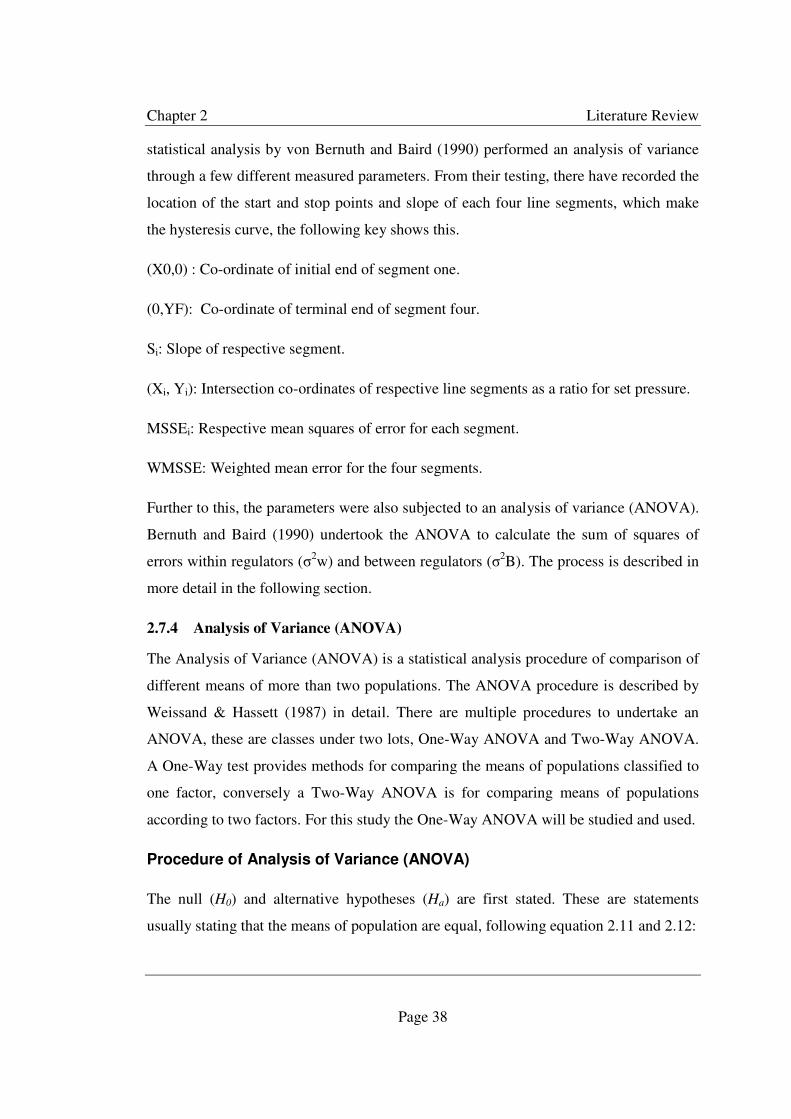
Chapter 2 Literature Review
Page 38
statistical analysis by von Bernuth and Baird (1990) performed an analysis of variance
through a few different measured parameters. From their testing, there have recorded the
location of the start and stop points and slope of each four line segments, which make
the hysteresis curve, the following key shows this.
(X0,0) : Co-ordinate of initial end of segment one.
(0,YF): Co-ordinate of terminal end of segment four.
Si: Slope of respective segment.
(Xi, Yi): Intersection co-ordinates of respective line segments as a ratio for set pressure.
MSSEi: Respective mean squares of error for each segment.
WMSSE: Weighted mean error for the four segments.
Further to this, the parameters were also subjected to an analysis of variance (ANOVA).
Bernuth and Baird (1990) undertook the ANOVA to calculate the sum of squares of
errors within regulators (σ2w) and between regulators (σ2B). The process is described in
more detail in the following section.
2.7.4 Analysis of Variance (ANOVA)
The Analysis of Variance (ANOVA) is a statistical analysis procedure of comparison of
different means of more than two populations. The ANOVA procedure is described by
Weissand & Hassett (1987) in detail. There are multiple procedures to undertake an
ANOVA, these are classes under two lots, One-Way ANOVA and Two-Way ANOVA.
A One-Way test provides methods for comparing the means of populations classified to
one factor, conversely a Two-Way ANOVA is for comparing means of populations
according to two factors. For this study the One-Way ANOVA will be studied and used.
Procedure of Analysis of Variance (ANOVA)
The null (H0) and alternative hypotheses (Ha) are first stated. These are statements
usually stating that the means of population are equal, following equation 2.11 and 2.12:

Chapter 2 Literature Review
Page 39
RS: K4 = K5 = KU
2.11
RF: K4 ≠ K5 ≠ KU
2.12
Next the test statistic in question must be calculated, it is a ratio of variances between
and within treatments. It is calculated as the quotient of the treatment mean square
(MSTR) and error mean square (MSE).
� �� ��������E = *WX�*W�
2.13
where:
*WX� = WWX�Y − 1
2.14
*W� = WW�# − Y
2.15
where:
n is the total number of pieces of sample data and k denotes the population being
sampled and Treatment sum of square (SSTR) is calculated by equation 2.16 and error
mean square (MSE) is calculated by equation 2.17.
WWX� = #4�x1̄ − x̄�5 + #5�x2̄ − x̄�5 + ⋯ + #]�xk̄ − x̄�5 2.16

Chapter 2 Literature Review
Page 40
*W� = �#4 − 1��45 + �#5 − 1��5
5 + ⋯ + �#] − 1��]5 2.17
The next step is to decide on a significance level from this then the critical value (Fα) is
taken from the F-distribution. If the test statistic is greater than the critical value, the null
hypothesis is rejected, and for a test statistic less than the critical value the null
hypothesis is accepted.
(Weiss 1987)

Chapter 2 Literature Review
Page 41
2.8 Physical Analysis of Individual Components of Pressure Regulator
2.8.1 Introduction
A pressure regulator is a device which consists of different individual components
which work in conjunction with each other to perform is designed function – to output a
constant outlet pressure regardless of the input pressure. A physical analysis should be
made of the individual components which contribute to the overall workings of the
pressure regulator. The individual components within the pressure regulator include the
spring and O-ring.
2.8.2 Spring
A mechanical spring is defined has an elastic body whose primary function is to deflect
or distort under load (or to absorb energy) and which recovers its original shape when
released after being distorted (Wahl 1963). Within the pressure regulators the spring is
an important component; it counteracts the force being provided by the back pressure, to
move the tube to its correct position in order to give the variable headloss. There are
many different types of springs, and depending on the application will determine the
specific type needed. The type of spring used in the pressure regulators are a helical
compression or tension spring. These types of springs are the most widely type used and
are made from wire coiled to form a helical shape. The load applied is transformed
along the helical axis of the spring. Figure 2.13 below illustrates a helical spring with
the load and dimensions. Figure 2.14 shows the dimensions from the top view of the
spring.
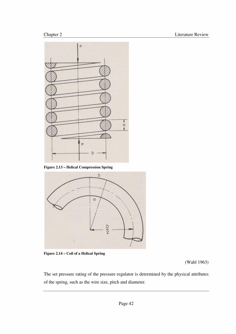
Chapter 2 Literature Review
Page 42
Figure 2.13 – Helical Compression Spring
Figure 2.14 – Coil of a Helical Spring
(Wahl 1963)
The set pressure rating of the pressure regulator is determined by the physical attributes
of the spring, such as the wire size, pitch and diameter.

Chapter 2 Literature Review
Page 43
When a spring is used either in compression or tension the force it exerts is proportional
to its change in length. This phenomena is known as Hooke’s Law which is the
following equation,
= = −Y� 2.18
where: F is the resultant vector force, k is the spring constant and x is the displacement
of the spring (A Hooke’s Law Spring 2008).
2.8.3 O-ring
An O-ring functions as a seal. It seals by physical deformation of the O-ring. An O-ring
is usually made out of an elastic material such as rubber. Figure 2.15 below shows a
typical O-ring and the characteristic dimensions.
Figure 2.15 – O-ring Dimensions
(O-Ring Gland Design Charts 2003)
Within the pressure regulator there are two O-rings, both which are seated on the top of
the internal casing. The larger O-ring seals the internal casing and the redistribution plug
and stops any fluid going outside the area. The second O-ring fits in a moulded seat,
with the tube moving up and down through the O-ring. This area is filled with water
when in operation. As discussed in earlier sections, the hysteresis effect in the pressure
regulator is caused by the mechanical friction of the tubes movement though the O-ring.
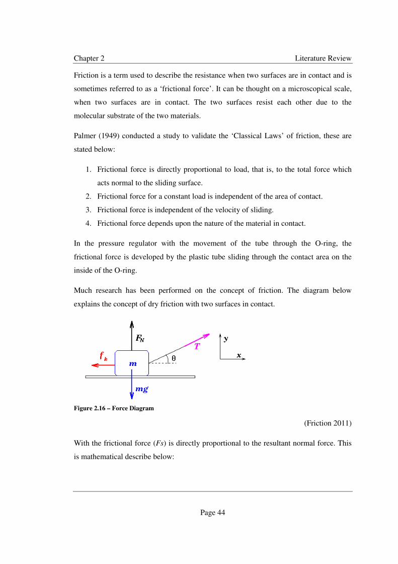
Chapter 2 Literature Review
Page 44
Friction is a term used to describe the resistance when two surfaces are in contact and is
sometimes referred to as a ‘frictional force’. It can be thought on a microscopical scale,
when two surfaces are in contact. The two surfaces resist each other due to the
molecular substrate of the two materials.
Palmer (1949) conducted a study to validate the ‘Classical Laws’ of friction, these are
stated below:
1. Frictional force is directly proportional to load, that is, to the total force which
acts normal to the sliding surface.
2. Frictional force for a constant load is independent of the area of contact.
3. Frictional force is independent of the velocity of sliding.
4. Frictional force depends upon the nature of the material in contact.
In the pressure regulator with the movement of the tube through the O-ring, the
frictional force is developed by the plastic tube sliding through the contact area on the
inside of the O-ring.
Much research has been performed on the concept of friction. The diagram below
explains the concept of dry friction with two surfaces in contact.
Figure 2.16 – Force Diagram
(Friction 2011)
With the frictional force (Fs) is directly proportional to the resultant normal force. This
is mathematical describe below:
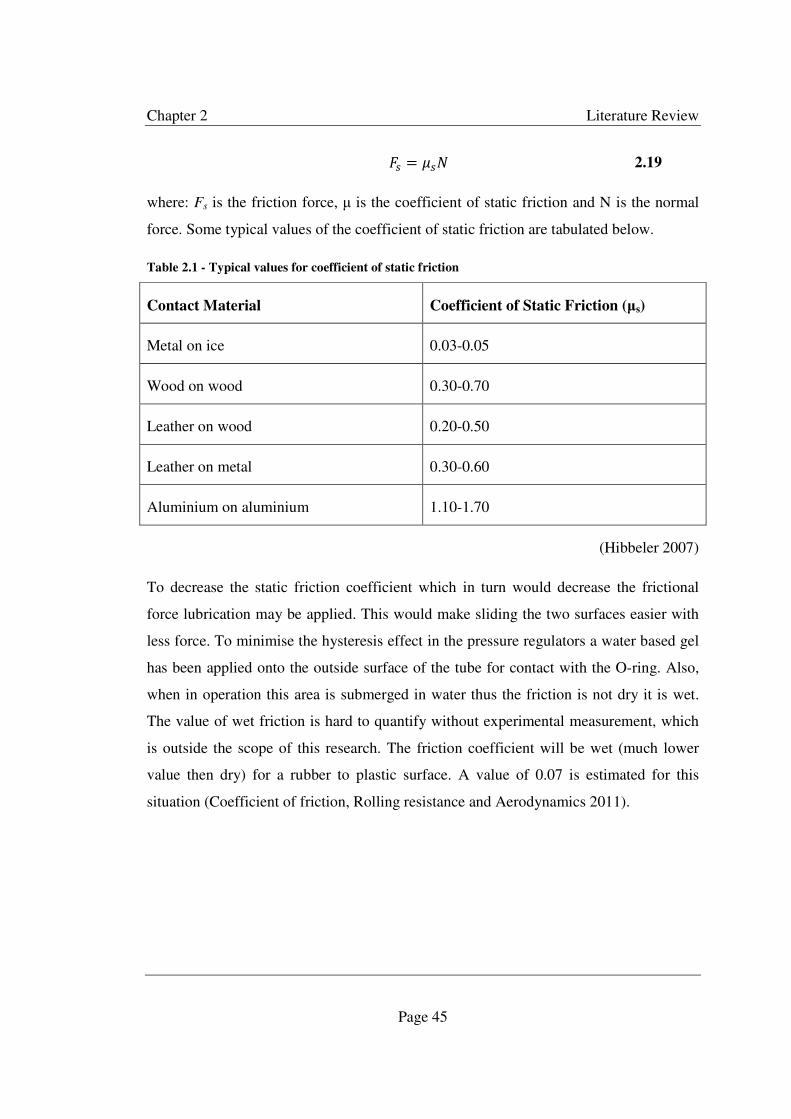
Chapter 2 Literature Review
Page 45
=_ = K_` 2.19
where: Fs is the friction force, µ is the coefficient of static friction and N is the normal
force. Some typical values of the coefficient of static friction are tabulated below.
Table 2.1 - Typical values for coefficient of static friction
Contact Material Coefficient of Static Friction (µs)
Metal on ice 0.03-0.05
Wood on wood 0.30-0.70
Leather on wood 0.20-0.50
Leather on metal 0.30-0.60
Aluminium on aluminium 1.10-1.70
(Hibbeler 2007)
To decrease the static friction coefficient which in turn would decrease the frictional
force lubrication may be applied. This would make sliding the two surfaces easier with
less force. To minimise the hysteresis effect in the pressure regulators a water based gel
has been applied onto the outside surface of the tube for contact with the O-ring. Also,
when in operation this area is submerged in water thus the friction is not dry it is wet.
The value of wet friction is hard to quantify without experimental measurement, which
is outside the scope of this research. The friction coefficient will be wet (much lower
value then dry) for a rubber to plastic surface. A value of 0.07 is estimated for this
situation (Coefficient of friction, Rolling resistance and Aerodynamics 2011).

Chapter 3 Materials and Methodology
Page 46
Chapter 3 MATERIALS AND METHODOLOGY
3.1 Introduction
A crucial component of this research work and perhaps the most important, taking the
majority of the time, was to develop a suitable and appropriate testing methodology
which gave repeatable robust results. There has been no previous research work which
describes a correct testing methodology to characterise the performance of pressure
regulation devices used in broad-acre irrigation. Different approaches were used to try
and achieve the repeatability and to present the raw data in such a way which would
accurately describe the performance characteristics and differentiate between
manufacturing variability, testing procedure and its actually real test bench performance.
To start the testing and to begin the first stage of the methodology the Hydraulics
Laboratory was used to setup the basic materials used in the methodologies.
3.2 Hydraulics Laboratory Experimental Setup
The University of Southern Queensland, Faculty of Engineering and Surveying’s
Hydraulics Laboratory has extensive infrastructure to perform and carry out hydraulic
testing and modelling. It was decided to carry out this projects tests and experimentation
in this laboratory.
3.2.1 Hydraulics Laboratory Constant Supply Header Tanks
Part of the hydraulics laboratory Z113 infrastructure is a low and high constant head
supply header tanks. Both header tanks have the capacity to deliver a constant supply of
head to the laboratory. The tanks are bolted onto the side of Z block. The tank’s design
has two sections, an inner and outer part. Water is pumped up into the inner section of
the tank via a 200 mm diameter polythene pipe. When the inner section of the header
tank fills it overflows into the out section of the tank. There are two more pipes
connected to the header tank, one pipe carries the spilled water in the outer section back
to the reservoir and the other pipe carries the inner section part of the tank to the
laboratory.

Chapter 3 Materials and Methodology
Page 47
The hydraulics laboratory reservoir is a 30, 000 litre tank which is situated underneath
the floor of the laboratory. Water is pumped up to the header tank, providing a constant
head supply to the experiment. The floor of the laboratory has been designed to be
drained, it is in sloped sections and allows water to drain back into the underground
reservoir.
The 200 mm supply line from the high header tank delivers the supply to the back of the
hydraulics laboratory with three outlets. A butterfly valve is connected to each outlet.
This provides the water supply to the experiment setup. There are separate lines each
from the low and high header tanks.
To understand the exact pressure being provided to the experiment it was decided
necessary to perform a level run survey from a fixed point in the laboratory where the
testing was being performed up to both header tanks. This would give millimetre
accuracy on the vertical height of the constant supply level in each header.
To perform this survey a Leica automatic level was borrowed from the surveying
department of the University of Southern Queensland, along with a staff, tripod and
bubble for the level. The Leica automatic level was setup on the tripod and levelled
using the three footscrews, with the help of a staffman, a backsight reading was taken
and recorded. It was made sure that when all readings were taken, the staff was held
perpendicular by the staffman from reference with the bubble. Keeping the distances
between readings similar to minimise error a foresight reading was taken and recorded,
the instrument was then moved to a new location and the points booked. The level run
went from a specified point near the testing rig to the weir lips on both high and low
header tanks. This was done by three different level runs from and back to known
points. Appendix E shows the booking sheet for the three separate surveys, the surveys
have been booked down the page. From the survey it was calculated the elevation
difference between the low and high header tanks and the specified point near the test
rig is 6.390 metres and 16.181 metres respectively with +/- 0.001 metre accuracy.
Chapter 3 Materials and Methodology
Page 48
3.3 Test Rig and Kit
3.3.1 Introduction
As with many research and experimental projects many different components are used
in formulating the kit used in the experiment. This project was no different as it used
many different components in the test rig.
3.3.2 Experiment Discharge Measurement
The flowmeter selected for this experiment was an ABB Instrumentation MagMaster
HA3 Electromagnetic Flowmeter. The flowmeter’s serial number is P/23730/1/1. This
flowmeter has a 15 mm bore size and two flange fittings for the inlet and outlet of the
flowmeter. The flange fittings were specially made to bolt into the flowmeter’s inlet and
outlet with a male 12.7 mm end connecter being able to be threaded into these flanges.
The rated accuracy for this model is +/- 0.15%. This flowmeter was purchased some
years ago, however has not been used. The experiment is the first usage of the meter
since purchase.
3.3.3 Experiment Pressure Measurement
Pressure measurement in this project was both manual and automated. For some stages
of pressure measurement, pressure gauges were used. These gauges are WIKI fluid-
dampening pressure gauges, with a reading accuracy of +/- 0.5 %. The inlet pressure
measurement was taken with a gauge which ranged from 0 to 600 kPa with 10 kPa
increments and the outlet pressure gauge ranged from -100 to 300 kPa with 5 kPa
increments (the negative reading being vacuum pressure, which was not valid in this
experiment, but the gauge still used).
With automation testing, pressure transducers were needed to be included in the test rig.
The pressure transducers used were a Druck PMP 4030 type. Two transducers were used
in the experimental kit, one upstream of the pressure regulator measuring the input
pressure and one downstream of the pressure regulator measuring the output pressure.
Because from these two different positions there would be unregulated pressure and
regulated pressure (upstream and downstream respectively) two different pressure
Chapter 3 Materials and Methodology
Page 49
ranges were used. For the upstream readings a 0 to 400 kPa pressure transducer was
used and for the downstream readings a 0 to 250 kPa pressure transducer was used. The
serial numbers of these Druck PMP 4030 pressure transducers were 1833125 and
1820216 respectively. A 12 volt DC regulated power supply was used to power the
pressure transducers. The specifications give the standard accuracy of these pressure
transducers as +/- 0.08% FS (Full scale) BSL (Best straight line).
3.3.4 Experiment Pipes, Fittings and Valves
The plumbing of the experimental test rig was based on using 19.0 mm polythene pipe.
The reason for this was that the standard size of the pressure regulators being tested was
19.0 mm and also that the pipe fittings for this size were relatively available. For most of
the testing the flowmeter was directly plumbed from the supply, this line then continued
on to the experiment test rig. A specially built table was designed and built for the
testing. This table separated and contained the wet from the dry side of the experiment.
The computer monitor, keyboard, mouse and valve levers were operated from the top
and underneath housed the pressure regulator being tested with the necessary fittings
and valves.
Measuring the pressure, the pressure transducers were tapped into the line via two
tapping saddles one upstream and one downstream of the pressure regulator. 6 mm
barbed fittings were then fitted into these tapping saddles with 6 mm plastic tubing
connected back to the top of the table were the pressure transducers were placed. The
elevation difference between the pressure transducer and the tapping point was always
accounted for in the processing of the raw data.
Two valves were used in this experimental testing rig one upstream and one downstream
of each pressure transducer tapping point. The two valves were used in conjunction with
each other and were an integral part of the testing rig. The valves used were a Belimo
R218 type. These valves had a special insert inside them which meant their headloss
coefficient (K), no matter the stage the valve was turned would always be 1.
Chapter 3 Materials and Methodology
Page 50
3.3.5 Electronic Data Acquisition
As part of the automation process, the flowmeter and the two pressure transducers were
connected to a data acquisition board (DAB). This took the signal being produced by the
three sensors and converted it to a voltage were it was read by the computer software.
The pressure transducers were wired up into the DAB with the power, ground and signal
wires into their specified positions. The signal produced by the pressure transducers was
a signal voltage. The specifications state that for the upstream pressure transducer (0 to
400 kPa) the signal voltage ranges from 0 to 5 volts; whereby if the signal being
received is 5 volts this is 400 kPa being experienced by the sensor in the pressure
transducer. Similarly for the downstream pressure transducer (0 to 250 kPa) its signal
ranges from 0 to 5 volts so at 5 volts the pressure transducer is sensing 250 kPa. These
were the uncalibrated theoretical readings.
The ABB MagMaster flowmeter outputs a similar signal however the signal output is a
current signal not voltage. This signal is a 4 to 20 milliamp output for a 0 to 0.9 L/s flow
range. For the DAB and software to read this the signal needed to be converted to a
voltage signal.
� = a�
where: V = voltage (volts), I = current (ampere) and R = resistance (ohm)
3.1
From equation 3.1 it can be seen the relationship between voltage and current. To obtain
a voltage for a 1 to 5 volt range from the 4 to 20 milliamp current signal from the
flowmeter, a 250 ohm resistor is used. The signal being converted needed to maintain
high precision, thus a special resistor was used for this conversion. The resistor used was
a Vishay ultra high precision Z201 Z-foil 250 ohm resistor, which had a standard
tolerance value of +/- 0.005%.
3.3.6 Labview: The Data Acquisition Software
From the data acquisition board these signals were connected into a computer. The
program Labview was used to write a program which read the signal voltages from the

Chapter 3 Materials and Methodology
Page 51
flowmeter and two pressure transducers and displayed these on an interface. This
program was created by Dean Beliveau of the University of Southern Queensland for
this project. Labview was the program which is loaded and used for the automation
tested. The program has the capacity to output text files where each line being outputted
is an average of 20 readings taken over one second. This is due to the 20 Hz cycle which
the DAQ and labview is setup. Each line (each second) has a discharge, input pressure
and output pressure recorded respectively along with a data and time stamp every time
the program is hit to record.
3.4 Calibration of Electronic Measurement Devices
Undertaking scientific measurements using electronic measurement apparatus, an
understanding of the accuracy, repeatability and limitations of the devices needs to be
known, in order to know the accuracy of the readings. This study is no different in terms
of this need, in fact the understanding of the limitations of the measuring devices help to
understand and interpret the raw data. With this project there are two main
measurements taken, discharge and pressure. High accuracy was needed to understand
the small differences between measurements
3.4.1 Flowmeter Calibration
The flowmeter was calibrated before purchase on the 20th July 2003. The calibration
was taken place at a Narda accredited facility. The certificate of calibration for this
electromagnetic flowmeter is included in Appendix D.
3.4.2 Pressure Transducer Calibration
The pressure transducers did not come with a certified calibration certificate from the
supplier, thus less confidence was placed on its stated accuracy limit. An independent
calibration of the pressure transducers was needed to confirm the accuracy and linearity
of the measurement device.
To begin this calibration process a Dead Weight Pressure Tester (DWPT) was used. The
DWPT consisted of a hydraulic loading cylinder. Within this loaded area there is an
opening to place a tapping point; the pressure transducer (or other pressure device being

Chapter 3 Materials and Methodology
Page 52
calibrated) is placed. Also within the same loaded area another tapping point is fixed,
however this point is closed. Weights are loaded into this rod (which is fixed within a
casing in this point) and it rises up and down depending on the load placed by the
hydraulic cylinder. To load the DWPT a wheel was turned which directly pushed a
piston forward and placed a load on the two tapping points. When the rod was raised
with the weight, it equalled the same pressure applied on the pressure transducer. Figure
3.1 – Dead weight pressure tested calibrating the pressure transducers shows the DWPT
setup.
Figure 3.1 – Dead weight pressure tested calibrating the pressure transducers
This calibration testing took place on the 28th of February 2011. Oil was the fluid being
used to calibrate the pressure transducers, which is fine, however it is a more viscous
fluid compared to water and harder to get all air out of the system. The pressure
transducers, data acquisition board, and computer was taken to the DWPT and set up.
The 4.0 bar pressure transducer was used to be calibrated through the DWPT first. This

Chapter 3 Materials and Methodology
Page 53
transducer was filled with hydraulic fluid with an adaptor fitted; carefully this is
attached to the pressure tapping point on the DWPT making sure no air was entrapped
within the fitting. A ‘5 PSI’ rated weight was placed onto the rod which is lifted when 5
PSI of pressure is applied. The mass of the weight was not known or taken, as it already
has a rating placed on it. With the computer and Labview turned on and the data
acquisition board active the test was began. Slowly a load is placed onto the pressure
transducer by turning the wheel around to push the piston forward. Small movements
were given and when the rod pushed upwards the applied load was stopped. The rod
with the weight on top was spun around to make sure no viscous friction was pulling
back on the rod and that it was only under the influence of the load induced by the
hydraulic cylinder. The pressure displayed by labview was then recorded, as well as the
signal voltage transmitted by the pressure transducer into the data acquisition board
against this rated ‘5 PSI’ weight. A fluke 110 series digital multimeter was used to
measure the signal voltage output. The load was then backed off and an extra 5 PSI load
weight added and the process repeated. Increments of 5 PSI were tested up to 55 PSI for
the 4.0 bar pressure transducer and 35 PSI for the 2.5 bar pressure transducer. The
elevation difference between the pressure transducer sensor and the top of the rod was
measured for both transducers and used in the calculations to get the correct gauge
pressures for calibration.
After discrepancies in the calibration of the pressure transducers with this method using
the DWPT, a second means of calibration for the pressure transducer was needed.
This second calibration used an electronic way of calibration. To do this a Druck DPI
880 multi-function calibrator was used, connected into this was a Druck PV211
Pneumatic pressure and vacuum pump.
To calibrate, the pressure transducer was fitted into the pneumatic pressure pump and
used to pump up to a particular pressure. The fine adjustment was used on the side of the
pump to slightly increase or decrease the pressure. The pressure being produced by this
pump is experienced by both the pressure transducer and the Druck multi-function
calibrator. Making sure that the level of the sensors in both devices were the same, the

Chapter 3 Materials and Methodology
Page 54
pressure read by the Druck multi-function calibrator was recorded and the
corresponding voltage was measured using a fluke 110 series multimeter. The accuracy
for this multimeter for the reading of DC voltage is +/- 0.5%. A number of different
measurements were taken over the 0-5 signal voltage range; five different repeats were
done for the two different pressure transducers.
This electronic calibration while it did give better repeatability results then the DWPT,
the calibration still was not good enough for the level expected. After two methods of
using an electronic and mechanical means to read a corresponding pressure from the
pressure transducer and comparing to the calibration method to calibrate, it was decided
to use the header tank setup as a third very accurate method for calibration.
The theory which stems from this is related to the equation 2.3. If the elevation, density
and gravitational acceleration variables are known or are calculated or measured with
high accuracy then the static pressure would be also accurate. With the existing
infrastructure with the hydraulics laboratory there are two header tanks, a low tank and
high tank. With these two measurements from the header tanks and taking a third
smaller measurement of around 1.5 metres at ground level, this would cover the pressure
transducers operational range and give a highly accurate calibration in the form of a
linear equation which could be inputted into the Labview software which would take the
pressure transducers signal voltage and calculate the ‘real’ pressure and display it
through Labview.
A level survey between the low and high header tanks and the point of calibration in the
laboratory had been performed; this has been explained in section 3.2.1. This gives a
very accurate elevation difference between these two points. With the pressure
transducer sitting on the floor (the point where the level run was taken to) the diameter
of the pressure transducer was measured with a set of verniers with 0.002 mm reading
accuracy. The sensor of the pressure transducer is assumed to be in the centre of the
pressure transducer, so the radius of the pressure transducers was taken away from the
elevation difference between the low and high header tanks for the calibration process.
For the very low head measurement the column of water was measured with a tape
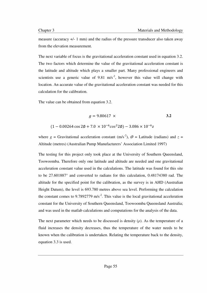
Chapter 3 Materials and Methodology
Page 55
measure (accuracy +/- 1 mm) and the radius of the pressure transducer also taken away
from the elevation measurement.
The next variable of focus is the gravitational acceleration constant used in equation 3.2.
The two factors which determine the value of the gravitational acceleration constant is
the latitude and altitude which plays a smaller part. Many professional engineers and
scientists use a generic value of 9.81 m/s-2, however this value will change with
location. An accurate value of the gravitational acceleration constant was needed for this
calculation for the calibration.
The value can be obtained from equation 3.2.
7 = 9.80617 ×
�1 − 0.00264 cos 2∅ + 7.0 × 10OiE�52∅� − 3.086 × 10Oi9
3.2
where g = Gravitational acceleration constant (m/s-2), Ø = Latitude (radians) and z =
Altitude (metres) (Australian Pump Manufacturers’ Association Limited 1997)
The testing for this project only took place at the University of Southern Queensland,
Toowoomba. Therefore only one latitude and altitude are needed and one gravitational
acceleration constant value used in the calculations. The latitude was found for this site
to be 27.601887° and converted to radians for this calculation, 0.48174380 rad. The
altitude for the specified point for the calibration, as the survey is in AHD (Australian
Height Datum), the level is 693.780 metres above sea level. Performing the calculation
the constant comes to 9.7892779 m/s-2. This value is the local gravitational acceleration
constant for the University of Southern Queensland, Toowoomba Queensland Australia;
and was used in the matlab calculations and computations for the analysis of the data.
The next parameter which needs to be discussed is density (ρ). As the temperature of a
fluid increases the density decreases, thus the temperature of the water needs to be
known when the calibration is undertaken. Relating the temperature back to the density,
equation 3.3 is used.

Chapter 3
) #���J =
This equation is based off a polynomial trend line fit to data.
relationship between the density of water and the temperature of the water, the equation
is seen on this graph.
sourced from The Engineering ToolBox (2011).
Figure 3.2 – Relationship between density and temperature for water
While the load was applied on the pressure transducer the signal voltage g
pressure transducer was measured. Making sure high accuracy reading
digital multimeter with a six digit readout was used. 34401A was the model of this
multimeter used. The calibration certification for this multimeter is
F; it was calibrated on the 21
With high accurate values known, the points for the low level
two header tanks were plotted for both the 2.5 and 4.0
regression line was plotted between these three points and the
the 2.5 and 4.0 bar pressure transducers was found. These equations are given below.
Materials
Page 56
�0.004 c X �. ���� 5 8 0.001 c X �. ����
This equation is based off a polynomial trend line fit to data.
relationship between the density of water and the temperature of the water, the equation
is seen on this graph. The data which has been graphed in figure
sourced from The Engineering ToolBox (2011).
Relationship between density and temperature for water
While the load was applied on the pressure transducer the signal voltage g
pressure transducer was measured. Making sure high accuracy reading
digital multimeter with a six digit readout was used. 34401A was the model of this
used. The calibration certification for this multimeter is
it was calibrated on the 21st April 2011.
With high accurate values known, the points for the low level measurement
two header tanks were plotted for both the 2.5 and 4.0 bar pressure transducers
plotted between these three points and the calibration
the 2.5 and 4.0 bar pressure transducers was found. These equations are given below.
Materials and Methodology
X �. ���� 8 1000 3.3
This equation is based off a polynomial trend line fit to data. Figure 3.2 shows the
relationship between the density of water and the temperature of the water, the equation
The data which has been graphed in figure Figure 3.2 has been
While the load was applied on the pressure transducer the signal voltage given from the
pressure transducer was measured. Making sure high accuracy readings were kept, a
digital multimeter with a six digit readout was used. 34401A was the model of this
used. The calibration certification for this multimeter is included as appendix
measurement and for the
ar pressure transducers. A linear
calibration equations for
the 2.5 and 4.0 bar pressure transducers was found. These equations are given below.
Chapter 3 Materials and Methodology
Page 57
For the 4.0 bar pressure transducer equation 3.4 is shown and equation 3.5 is given for
the 2.5 bar pressure transducer.
<� ���� �Y<�� = 80.107268 c W�7#� ���7 � 1.004808 3.4
<� ���� �Y<�� = 52.891850 c W�7#� ���7 � 6.033053 3.5
These equations were put into Labveiw for a direct calibration and the values output
from labview then only needed the elevation difference accounted for. However for the
early testing the equations were used in matlab to convert the pressures back to real
pressures.

Chapter 3 Materials and Methodology
Page 58
3.5 Function of the Nelson 10 PSI Pressure Regulator
Not much literature has been written on the working of pressure regulators used in
pressurised irrigation. To gain an understanding about the internal workings and
functionality of the pressure regulator, the device was dissembled, measured and drawn
to firstly understand how the device performs its designed function.
The pressure regulators task is to maintain a set output pressure, no matter the change in
input pressure, from this it could be said the device is a variable headloss, in constant
change to keep the set output pressure. A typical device used on LMIM is Nelson UNI-
Flo 10 PSI pressure regulator. To dissemble this device, six phillips head screws were
removed. There are five main components within the device, spring, tube, redistribution
plug, internal casing and two section of the external casing.
Tracking the movement of water through the pressure regulator the function of the
pressure regulator can be understood. Water is entered into the pressure regulator via the
input connection of the device. The first component in the pressure regulator which is
encountered is the redistribution plug. The redistribution plug’s purpose is to break the
streamline flow of the water as experienced through the input of the regulator. In the
Nelson UNI-Flo type regulator the redistribution plug is designed to allow the flow to go
through the plug. There is an obstruction in the centre of the plug; this obstruction is
attached to the edge of the plug. On the underside of this obstruction is a downward lip.
The next component in the pressure regulator past the redistribution plug, is the tube –
the main component in the device. The inlet of this tube is slightly angled outwards,
which draws the flow into the tube. The tube moves upwards and downwards depending
on factors happening at the other end of the tube. The position of the inlet of the tube in
relation to the downward lip of the redistribution plug forms the basis of the variable
pressure loss of variable headloss of the pressure regulator.
Once in the tube the flow passes down the length of the tube and is discharged into the
second half of the external casing of the pressure regulator. Where the outlet of the tube
is inserted into the external casing there is 0.3 mm clearance between the outside

Chapter 3 Materials and Methodology
Page 59
diameter of the tube and the casing. On the end of the tube there is six indentations into
the base of the tube, this allows some the fluid being discharged to be passed around the
outside of the tube and fill the void between it and the external casing. One of the
indentations has an opening cut which goes down the outside edge of the tube towards
the middle and then out bottom side of the base which has the rubber skirt around the
circumference of this base. Once the water enters into this area it pressurises and forms a
force which acts on the tube upwards.
The tube is fixed inside an internal casing. As shown in appendix B inside the internal
casing encases the spring. The two ends of the spring are seated in the internal casing,
the spring chamber, one side of the spring seated on the upstream side of the diaphragm
skirt and the other on the downstream side of the spring chamber. It is this seating of the
spring which provides a good transformation of the forces provided by the spring. When
the device is not in operation the spring pushes the tube in its furthest possible position.
It is then these two forces which form the basis of the resultant force to position the tube
to regulate.
To seal all the parts of the pressure regulator, rubber O-rings are used. As mentioned
above the rubber skirt is one seal which provides a flexible seal between the second part
of the external casing and the bottom of the internal casing. The second seal is a
typically O-ring. This seals fits onto a sit on the top of the internal casing. The
redistribution plug is installed on top of the casing. This stops water going down the
outside of the internal casing and filling the void between it and the external casing. The
third O-ring, is of more interest to knowing the performance of the pressure regulator. It
has a smaller diameter then the second O-ring described. It also fits into a moulded sit
on top of the internal casing. The tube then fits up into it. It provides a stable working
platform for the tube and keeps it parallel to the redistribution plug. As the tube moves,
there is a frictional forces between it and the O-ring. It is this force which gives the
pressure regulator its hysteresis effect. To overcome the hysteresis, the manufacturer has
put lubricant onto the outside of the tube, to lower the frictional force.

Chapter 3 Materials and Methodology
Page 60
When all the components are fitted together and the seals in place, to overcome void
spaces becoming pressurised, vents have been included in the design. To vent the spring
chamber, there is a smaller cut away section within the internal casing. As mentioned
above, on the bottom of the tube, there six segments slightly shorted then the other six
segments. When in a fully open position, air is still able to get into the system. Both of
these incorporated designs allows the pressure regulator to function used atmospheric
pressure conditions and at no stage is the device able to build up pressure which would
affect the workings and functionality of the pressure regulator.
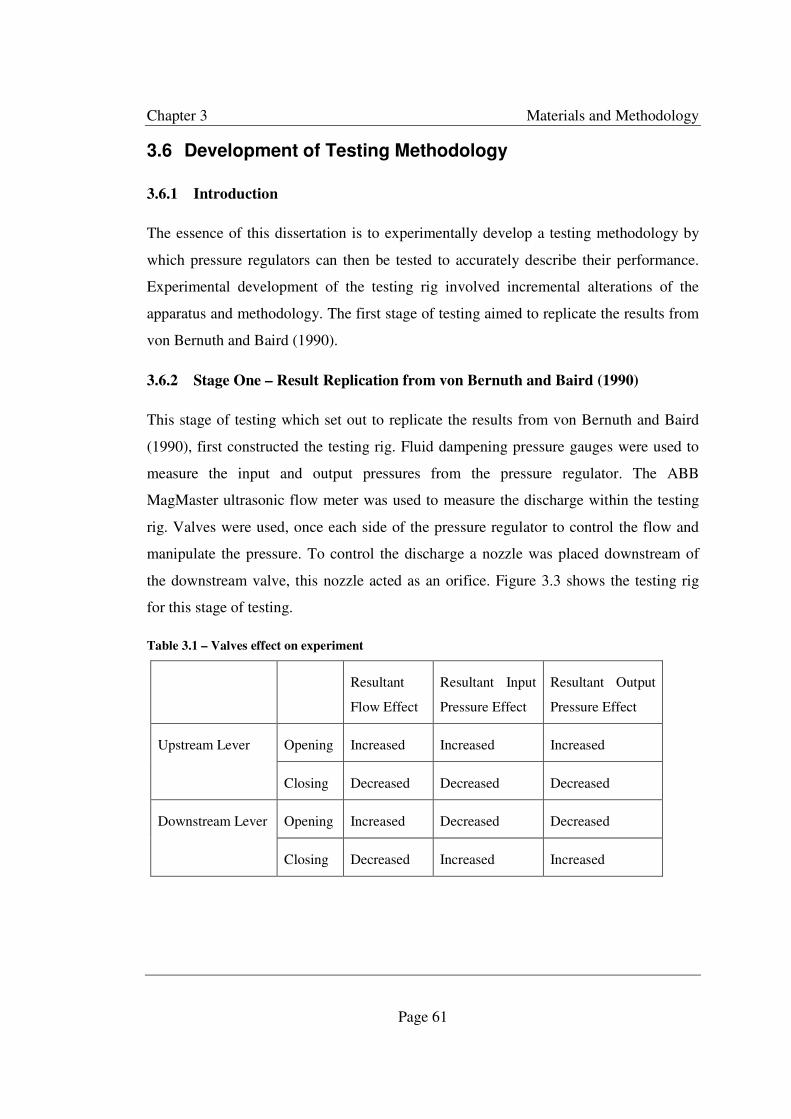
Chapter 3 Materials and Methodology
Page 61
3.6 Development of Testing Methodology
3.6.1 Introduction
The essence of this dissertation is to experimentally develop a testing methodology by
which pressure regulators can then be tested to accurately describe their performance.
Experimental development of the testing rig involved incremental alterations of the
apparatus and methodology. The first stage of testing aimed to replicate the results from
von Bernuth and Baird (1990).
3.6.2 Stage One – Result Replication from von Bernuth and Baird (1990)
This stage of testing which set out to replicate the results from von Bernuth and Baird
(1990), first constructed the testing rig. Fluid dampening pressure gauges were used to
measure the input and output pressures from the pressure regulator. The ABB
MagMaster ultrasonic flow meter was used to measure the discharge within the testing
rig. Valves were used, once each side of the pressure regulator to control the flow and
manipulate the pressure. To control the discharge a nozzle was placed downstream of
the downstream valve, this nozzle acted as an orifice. Figure 3.3 shows the testing rig
for this stage of testing.
Table 3.1 – Valves effect on experiment
Resultant
Flow Effect
Resultant Input
Pressure Effect
Resultant Output
Pressure Effect
Upstream Lever Opening Increased Increased Increased
Closing Decreased Decreased Decreased
Downstream Lever Opening Increased Decreased Decreased
Closing Decreased Increased Increased

Chapter 3 Materials and Methodology
Page 62
Once the test rig was constructed, testing began to try and replicate the results from von
Bernuth and Baird (1990) experiment. This involved getting different input pressure and
recording the output pressure at a constant discharge. Two pressure regulators were
tested a Valley 6 PSI and a Nelson 10 PSI. The pressure regulator was coupled into the
testing rig via two quick coupling fittings. A Nelson 3TN #48 nozzle was fitted at the
end of the pipeline within the test rig to maintain a constant discharge through the
system. The whole testing rig was flooded to ensure the system was free of air. In
replicating the results of von Bernuth and Baird (1990), the ‘hysteresis curve’ was tried
to be produced by obtaining multiple points around this curve. As described in chapter
two, hysteresis within the pressure regulator is due to the frictional force of the O-ring
against the movement of the tube. To get the points on the boundaries of the curve either
a rising or falling input pressure was needed.
With the high header tank system on the butterfly valve was turned on and the static
head was recorded from the fluid-dampened pressure gauge. The upstream and
downstream valves were then turned on allowing, water through the system. The
upstream valve was turned on 90% of the way. The downstream valve was then adjusted
to obtain the constant discharge value. For a rising pressure, being on the upper limb of
the hysteresis curve, it was made sure that the very last movement of either valve was to
get a rising. Similarly for a falling pressure, on the lower limb of the hysteresis curve, it
was made sure the last movement was to obtain a falling pressure. To get an accurate
and precious desired discharge requires very small adjustments on the levers on
upstream and downstream valves. Once the correct discharge was arrived at making sure
that the last movement of the two valves was to either get a rising or falling pressure
from the pressure regulator; the upstream and downstream pressures were read manually
off the WIKI pressure gauges and recorded. The flowmeter also was manually read and
recorded. Once multiple points had been obtained around the hysteresis curve, the
second pressure regulator was placed in the testing rig and tested. The raw data was
processed and graphed in Microsoft Excel. Figure 4.1 andFigure 4.2 show the results for
the result replication from the literature of von Bernuth and Baird (1990).

Chapter 3 Materials and Methodology
Page 63
Figure 3.3 – Stage one testrig Results replication from von Bernuth and Baird (1990)
3.6.3 Stage Two – Automatic data acquisition
Setting up the stage two testing rig took time, as the automation data acquisition needed
to be incorporated into the hydraulic setup. Section 3.3 details the materials used in
stage two testing and how stage one was further with the existing equipment such as the
flowmeter, valves and pipe fittings. Error! Reference source not found. shows the
testrig setup for this automatic data acquisition stage.
Once the testing rig for the automatic data acquisition was assembled, with all pipe Once the testing rig for the automatic data acquisition was assembled, with all pipe
fittings checked for leaks and the high header tank system on, the butterfly valve was
turned on and the experiments allowed to be flooded to allow air to escape from the
system.
Chapter 3 Materials and Methodology
Page 64
With the computer powered, the flowmeter turned on and the data acquisition board
with power, the program Labview was opened. The butterfly valve being opened gives a
constant level water supply to the experiment from the high header tank.
Figure 3.2 shows a red 25.4 mm gate valve attached to a galvanised dropper from the
flange attached to the butterfly valve. With the butterfly valve fully open, the red gate
valve allowed finer adjustment control of the discharge into the experiment. The first
discharge of interest is 0.05 L/s. To vary the input head the upstream lever was moved.
For a rising pressure the upstream lever was opened, this allowed the discharge to go
above the discharge band rate allowed in the labview program. To compensate the
downstream lever was closed very carefully and slowly. This brought the discharge back
into to the discharge of interest, while still the pressure was rising. The system was
allowed to settle for 3-5 seconds. The software was then allowed to record this point and
write it to a textfile. Multiple rising pressure points were obtained at this constant
discharge.
Falling pressure points were then obtained. To do this the upstream valve was adjusted
to get the discharge below its final value. The downstream valve was then opened to
move the discharge to its final value. This process was then repeated to obtain multiple
falling output pressure points. Another discharge value was tested for the rising and
falling pressures. For this stage of testing, automatic data acquisition discharges of 0.05
through to 0.3 L/s at 0.005 L/s increments and 0.5 L/s. At the start and end of each
discharge measurement the temperature of the water was measured by an alcohol filled
thermometer.

Chapter 3 Materials and Methodology
Page 65
Figure 3.4 – Stage two testrig Automatic data acquisition
Appendix G shows two output text files for this stage of testing of 0.30 and 0.50 L/s.
These output files have been taken straight from Labview. After the testing the textfiles
needed to be processed so the raw data can be presented in a way which is easier for
interpretation. To do this process matlab was used and appendix H shows the matlab
code which was used to take each textfile and brought it into matlab and processed the
discharges, input and output pressures.
When the testing was in progress and labview was allowed to recorded, occasionally
two seconds of data would be recorded, meaning two lines of data would be written to
the textfile. When the textfile was input into matlab, both lines of data have been
analysed and the discharge closest to the one of interest is accepted with their
corresponding input and output pressures. After all the data was taken from the textfiles
and put into matlab the pressure calibration was undertaken. Section 3.4.2 describes the
importance of calibration and details the process taken to calibrate the pressure

Chapter 3 Materials and Methodology
Page 66
transducers. When this testing was carried out, labview has the signal voltage for the
pressure transducers as a direct linear relationship, after calibration is was proved not to
be correct. The matlab code takes both the input and output pressures and converts them
back to signal voltages and then takes these signal voltages and runs it through the
respective calibration equation to arrive back to the correct pressures (kPa).
The water temperatures which were measured and recorded at the time of the test, these
were entered into the matlab and the corresponding densities were calculated by the
equation 3.3. The pressure offset from the tapping point into the experiment to the
position of the pressure transducer was also measured accurately and this was entered
into matlab. With all this information and the local gravitational acceleration constant
for Toowoomba was calculated from equation 3.2, and the pressure head was calculated.
Matlab was then used for plotting and its graphical editor feature utilised for easier
formatting of the matlab figures.
3.6.4 Stage Three – Automatic data acquisition with higher input heads
In this stage of testing saw the addition of a pump to the test rig. Figure 3.3 shows the
setup for this stage of testing. The 25.4 mm red gate valve used in stage two testing was
also used in stage three testing to give control over the discharge of the pump and
regulate the flow into the experiment. It is important to monitor the head going into the
experiment due to the pressure transducers. If too higher head was experienced while the
transducers are attached, this would damage the diaphragm in the transducer. Thus
before the pump was started the red gate valve was turned off. Appendix I shows this
Southern Cross HX-C pump’s performance curve. This stage of testing saw extra input
head added to simulate the input head that the pressure regulators experience in the field
on large mobile irrigation machines. A similar methodology was used in stage three has
in stage two tests.
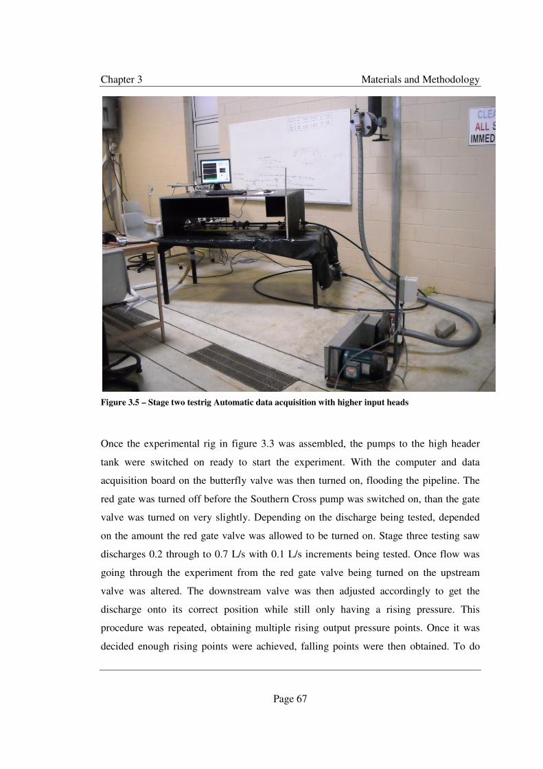
Chapter 3 Materials and Methodology
Page 67
Figure 3.5 – Stage two testrig Automatic data acquisition with higher input heads
Once the experimental rig in figure 3.3 was assembled, the pumps to the high header
tank were switched on ready to start the experiment. With the computer and data
acquisition board on the butterfly valve was then turned on, flooding the pipeline. The
red gate was turned off before the Southern Cross pump was switched on, than the gate
valve was turned on very slightly. Depending on the discharge being tested, depended
on the amount the red gate valve was allowed to be turned on. Stage three testing saw
discharges 0.2 through to 0.7 L/s with 0.1 L/s increments being tested. Once flow was
going through the experiment from the red gate valve being turned on the upstream
valve was altered. The downstream valve was then adjusted accordingly to get the
discharge onto its correct position while still only having a rising pressure. This
procedure was repeated, obtaining multiple rising output pressure points. Once it was
decided enough rising points were achieved, falling points were then obtained. To do
Chapter 3 Materials and Methodology
Page 68
this the upstream valve was adjusted just below the discharge of interest. The
downstream valve was then opened to arrive at the discharge for a falling pressure.
Again as with stage two a textfile is written which outputs the raw data from labview.
Appendix J shows the raw data output for this stage of testing for automatic data
acquisition with higher input heads for discharges of 0.2 and 0.4 L/s. A simular matlab
script as shown in appendix H was used for the analysis and processing of the raw data.
3.6.5 Stage Four – Continuing Valve Movement Test
In this stage of the testing procedure no major changes to the testing rig were seen,
however a different approach in how the testing rig was used to try and further the
understanding in how the pressure regulators function.
Stage four testing started by tracking the input head around the hysteresis curve and
using the two levers, up and downstream of the regulator, simultaneously in order to
keep the discharge in a tight band. Because the reading were continuous and not steady
like stages two and three, this meant that the discharge could not be a set constant. The
levers however provided good control and thus allowed for very small movements
which meant the smallest possible changes in discharge possible.
To begin this stage of testing the testing rig was configured as in stage three. With the
high header tank system turned on the butterfly valve was opened and the system
flooded. The Southern Cross pump was switched on and the red gate valve adjusted
according to the specific discharge being aimed. The first aimed discharge was 0.2 L/s.
With both the upstream and downstream levers which are attached to the corresponding
valves upstream and downstream of the pressure regulator in the fully shut position the
bandrate was entered into the labview software. The bandrate was 10% of the discharge
of interest. The levers were then altered to get the lowest possible input head while
maintaining the discharge. As with previous tests the water temperature was measured
and recorded before the beginning of the test. This began the starting point of the test,
and the software was then hit to record. The upstream lever was slowly opened to allow
extra input head into the system while keeping a close eye on the discharge trace not
Chapter 3 Materials and Methodology
Page 69
letting the flow going outside the specified band rate. The downstream lever was then
closed slightly, this raised the pressure but also increased the discharge which
compensated for the previous change of discharge, again the discharge was kept within
the band rate.
This tedious process continued to the maximum allowable input head which could be
received by the pressure transducer ≈ 400 kPa, this then was the rising pressure. While
the system was still recording the test then was in the falling pressure stage. The
upstream valve was slightly closed; again making sure the discharge did not go outside
the band rate. The downstream valve was then slightly opened which compensated for
the discharge change. The process continued until the input head was at the lowest
possible point for the discharge to be kept in the band rate. This whole process was then
repeated; however instead of going to 400 kPa, at each 50 kPa increment from 400 the
falling pressure was began. The software was allowed to record for this cyclic
measurements around the pressure regulators hysteresis curve.
Once difference approaches were taken from the upper to the lower limb of the
hysteresis for this aimed discharge of 0.2 L/s with the set bandrate of 10%, the test was
repeated for another aimed discharge of 0.4 L/s and 0.6 L/s. Matlab was used for the
processing of this data and analysis.
3.7 Creep test
A different approach was taken with this stage of testing, the creep testing. This stage
investigated the movement of the tube within the pressure regulator with the device is
functioning for a long period of time. To perform this test it was split into two sections,
a rising and falling section. Using the same testing rig and materials as in testing stages
two (automatic acquisition test), the computer and software was started up to begin the
test. As in stage two the high header tank was used as the supply to the experiment,
making sure there was no air in the supply line the butterfly valve was turned on. Using
the two levers simultaneously a rising input head was selected at a specified discharge.
Making sure the last move of the levers was a rising input head, either the upstream
lever was opened or the downstream lever was closed to get to the specified discharge.
Chapter 3 Materials and Methodology
Page 70
Once this point was arrived at the labview software was started to record. Both levers
and the butterfly valve was then not touched or altered. Immediately after the software is
started to record the temperature of the water passing through the experiment is
measured and recorded. The test was left to run for 24 hours. Every three to four hours
over the 24 hour period the temperature was measured and recorded and fed back into
the analysis for use with the raw data. After this 24 hour period the experiment was
stopped and the levers altered to arrive at a falling output pressure. Labview was then
left to record for 24 hours. The temperature of the water was measured every few hours
for both the rising and falling tests for analysis purposes.
3.8 Friction test
The same methodology was taken with this series of tests as the continuing valve
movement tests which is outlined in section 3.6.5. There were three sections to the
friction tests. The first stage, which is called normal lubrication, involved taking the
pressure regulator and testing it using the same procedure as described in section 3.6.5.
The pressure regulator was then dissembled and the lubrication wiped away from the
tube and the O-ring using a soft cloth, the pressure regulator was then resembled very
carefully and retested. This tested is referred to as no lubrication. After a second testing
the pressure regulator was dissembled and a water based lubrication was applied onto
the tube. The device was then retested and this test was referred to as extra lubrication.
Extra care was taken when dissembling and reassembling the pressure regulator and its
components between tests as damaging the tube could affect the performance of the
device.
Two pressure regulators were tested, both Nelson 10 PSI types, NL10-2 and NL10-3.
The NL10-2 was tested without the extra input head of the pump, only the high header
tank was used as the supply for the experiment. NL10-3 testing used the pump for obtain
extra input head for testing.

Chapter 3 Materials and Methodology
Page 71
3.9 Displacement of Tube inside Pressure Regulator
This stage involved tracking the movement of the tube inside the pressure regulator. The
movement of tube is the regulating component of the device, thus if a relationship can
be formed between this tracking movement and the other three parameters, discharge,
input and output pressures; a better understanding can be formed about the function of
the pressure regulator.
The methodology and materials used in stage six testing was different compared to
previous tests. The experiment was connected directly onto the flange connected to the
high header tank. From the 50 mm tee-piece coming off the flange fitting a valve was
fitted. This valve was the same type of valve used in previous experiments, only one
valve was used. The pressure regulator was fitted downstream of the value. To measure
the input and output pressures of the pressure regulator the tapping points were fitted
directly upstream and downstream of the pressure regulator using 19 mm polythene tee-
pieces. 6 mm tube was then connected back from these tapping points to the pressure
transducers and the elevation difference accounted for and recorded.
To measure the discharge a different set up needed to be constructed, as the experiment
needed to exit the pressure regulator via a nozzle which acted as an orifice under free
flowing conditions. The ABB MagMaster Ultrasonic flowmeter was used to measure the
discharge. To pass the flow through the flowmeter a meter length of 90mm PVC pipe
was plumbed into the inlet of the flowmeter with the appropriate reducing fittings to the
flowmeter’s 19.05mm threaded flange fitting. On the outlet side of the flowmeter, the
appropriate fittings were installed to a 90mm PVC pipe reducer. This creates a headloss
across the flowmeter. From the nozzle, the experiment is discharged directly into the 1
metre 90mm length attached to the inlet of the flowmeter. The high velocity being
discharged into the PVC length is dampened by the column of water held in the PVC
pipe. The water is then passed through the flowmeter by the head provided in the PVC
pipe. This forms the basis of the discharge measurement for this stage of testing. Figure
3.6 – shows the test rig for this testing stage.

Chapter 3 Materials and Methodology
Page 72
To track, gauge and measure the tube movements, non stretch was glued to the inside of
the tube with plastics glue. The fishing line used was a braid line, which provided
limited stretch and was a relatively easy material to glue to the tube. The tube is a very
smooth plastic material. To provide the adhesive Selleys Plastics Glue was used, this
was the only glue which could give a good bond to the smooth tubes surface.
The line was taken out of the experiment through the nozzle and threaded via two
pulleys; a weight was loaded on the other end of the line in the form of a bolt which
took the slack out of the line. When the supply to the pressure regulator is turned on and
an increasing input pressure is resulted on the tube moves forward to create a headloss
and regulate. Conversely when the supply is turned off and the input pressure is
decreased the tube moves backwards. Referring to appendix B, this action can be
visualised. When the tube moves either direction the load moves with it, to quantify this
movement a dial gauge is used.
A dial gauge is a measurement device used to determine small distances. The device
used for stage six testing is a Baty 10 mm travel length device with an increment step of
0.002 mm. A bolt is used at the load on the end of the line. On the bolt is a nut, by
holding the nut stationary and screwing the bolt a fine adjustment can be made of
placing the load onto the dial gauge. An indentation has been drilled into the head on the
bolt for the dial gauge to fit into. On the bottom of the bolt, a hole has been drilled and
treaded for an eye hook to screw into it. The line is tied to this eye hook. Two pullies are
used to shift the dial gauge and the load – the bolt away from the path of the jet of water
being discharged into the PVC pipe attached to the flowmeter. Figure 3.5 shows an
overview of stage six testing. Figure 3.6 shows the dial gauge setup in detail.

Chapter 3 Materials and Methodology
Page 73
Figure 3.6 – Testrig for Tubes movement

Chapter 3 Materials and Methodology
Page 74
Figure 3.7 - Dial gauge overview used for tubes movement
Beginning stage six testing, the valve is fully opened; this is to be the starting position
for the test. After the experiment has been assembled, the is valve turned on and the dial
gauge zeroed at this position; a video camera is set up in front of the dial gauge to record
its movement. The software is started and the data recording. A verbal start mark is
made, when the software is started to record. This is so make marrying up the two
separate datasets, the tubes movement and the software text file easier. The valve
situated upstream of the pressure regulator is then slowly turned on, taking at least 90
seconds to do this movement of the valve from fully open to fully shut. This process is
then repeated, however starting shut and going to fully open. This will move the tube
forward, taking load off the dial gauge, thus at time zero the dial gauge is loaded and the
position noted, the valve is then turned on slowly, while the software and camera both
record their corresponding articles. Two sized nozzles are tested, which give two

Chapter 3 Materials and Methodology
Page 75
different final valve discharge values. The nozzles used were the 3TN #15 and the 3TN
#28.

Chapter 3 Materials and Methodology
Page 76
3.10 Statistical Analysis Testing Methodology
This was the first and only series of tests which multiple pressure regulators were tested.
The high header tank was used as the supply for this experiment. The same equipment
setup was used in this series of tests as in automatic acquisition tests explained in
section 3.6.3.
To begin the test the computer and data acquisition board was all switched on. With
pumps running and high header tank system on the butterfly valve was fully opened.
The downstream valve was also fully turned on with the upstream valve fully off. With a
pressure regulator fitted in the test rig and all the air out of the system, Labview was hit
to record the upstream valve was then fully turned on and record stopped. Five repeats
were taken of this process before the pressure regulator was replaced and the process
repeated. 16 Nelson 10 PSI pressure regulators were tested. 5 had connection fittings 19
mm female to square and 11 had barbed to square (inlet to outlet fittings).
The last recorded line of data was used in the analysis process. Excel was for the data
analysis.
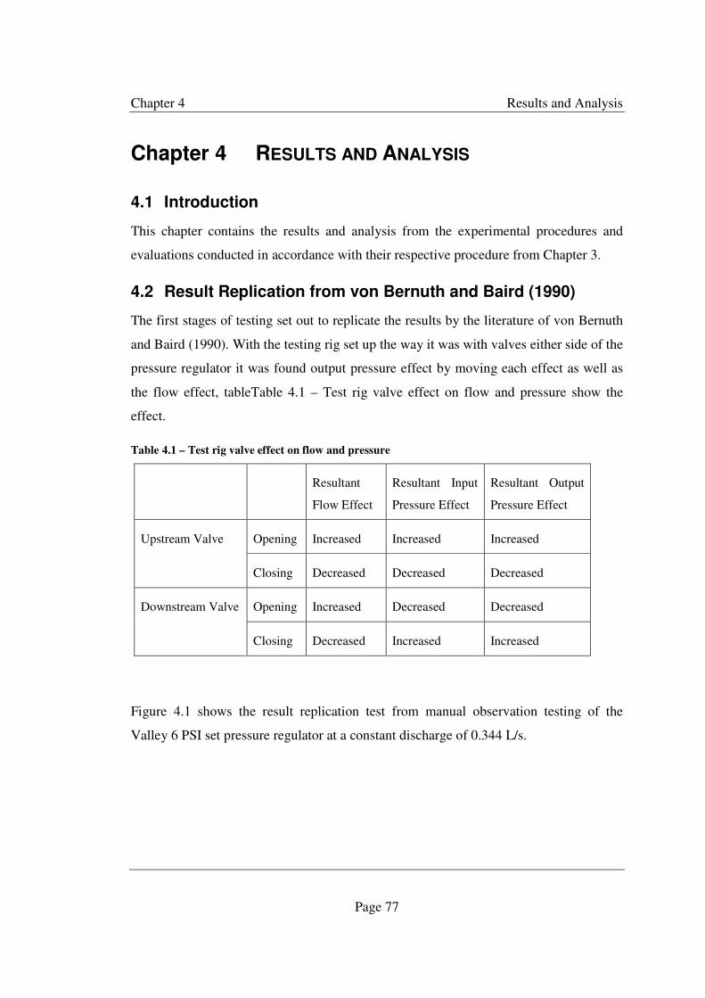
Chapter 4 Results and Analysis
Page 77
Chapter 4 RESULTS AND ANALYSIS
4.1 Introduction
This chapter contains the results and analysis from the experimental procedures and
evaluations conducted in accordance with their respective procedure from Chapter 3.
4.2 Result Replication from von Bernuth and Baird (1990)
The first stages of testing set out to replicate the results by the literature of von Bernuth
and Baird (1990). With the testing rig set up the way it was with valves either side of the
pressure regulator it was found output pressure effect by moving each effect as well as
the flow effect, tableTable 4.1 – Test rig valve effect on flow and pressure show the
effect.
Table 4.1 – Test rig valve effect on flow and pressure
Resultant
Flow Effect
Resultant Input
Pressure Effect
Resultant Output
Pressure Effect
Upstream Valve Opening Increased Increased Increased
Closing Decreased Decreased Decreased
Downstream Valve Opening Increased Decreased Decreased
Closing Decreased Increased Increased
Figure 4.1 shows the result replication test from manual observation testing of the
Valley 6 PSI set pressure regulator at a constant discharge of 0.344 L/s.
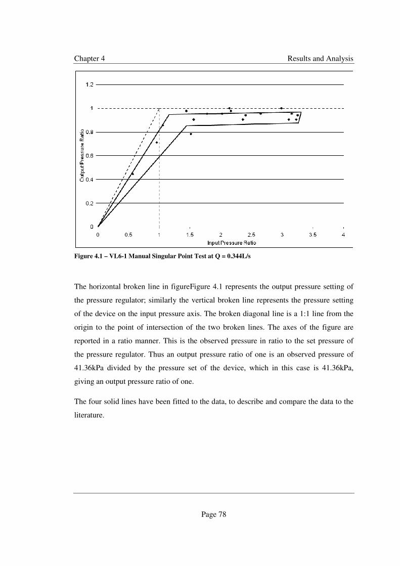
Chapter 4 Results and Analysis
Page 78
Figure 4.1 – VL6-1 Manual Singular Point Test at Q = 0.344L/s
The horizontal broken line in figureFigure 4.1 represents the output pressure setting of
the pressure regulator; similarly the vertical broken line represents the pressure setting
of the device on the input pressure axis. The broken diagonal line is a 1:1 line from the
origin to the point of intersection of the two broken lines. The axes of the figure are
reported in a ratio manner. This is the observed pressure in ratio to the set pressure of
the pressure regulator. Thus an output pressure ratio of one is an observed pressure of
41.36kPa divided by the pressure set of the device, which in this case is 41.36kPa,
giving an output pressure ratio of one.
The four solid lines have been fitted to the data, to describe and compare the data to the
literature.

Chapter 4 Results and Analysis
Page 79
Figure 4.2 - Nelson 10 PSI (NL10-1) Pressure Regulator Hysteresis Performance at Q = 0.344 L/s
Figure 4.2 shows a repeat of the testing, however with another pressure regulator, the
Nelson 10 PSI set pressure device with connection fittings threaded female to female.
The test was done at the same constant discharge as for the VL6-1 pressure regulator,
0.344 L/s. The unbroken lines represent the set pressure rating of the device and the axes
are pressure ratios. A different approach was taken with this test that the rising and
falling output pressure points have been plotted separately. The four solid line segments
were fitted to the rising and falling points. By doing this the four segments could be
better fitted to the data and a truer understanding be made of the hysteresis effect caused
by the internal friction of the tube on the O-ring. Without having the separation of the
rising or falling pressures the four segments were fitted manually for the Valley pressure
regulator test.
Table 4.2 – Comparison of manual singular point tests to published literature
S1 X0 S2 X0 Y2 S3 Y4 S4 YF

Chapter 4 Results and Analysis
Page 80
Literature
Ideal Value
1.000 0.000 0.00 1.0000 1.000 0.000 1.000 1.000 0.000
VL6-1 0.816 0.000 0.011 1.159 0.946 0.013 0.851 0.590 0.000
NL10-1 0.852 0.000 0.031 1.108 0.947 0.035 0.858 0.746 0.000
Table 4.2 show a comparison of the two pressure regulator tested, VL6-1 and NL10-1.
These values have been compared to the ideal values published from the literature of
von Bernuth and Baird (1990). It must be remembered that while both pressure
regulators were tested at the same constant discharge of 0.344 L/s, each pressure
regulator is of a different set pressure rating and different model. The compassion gives
an indication that the methodology of the testing does replicate the results to what the
literature describes as the ideal values for particular parameters. However the table does
show the NL10-1 performed truer to the literature ideal valves for most parameters. This
does not mean it necessarily has a better performance than the VL6-1 pressure regulator.
The parameters in the table refer to the slopes and start and end values of the four line
segments fitted to the data. FigureFigure 2.3 – Typical pressure regulator performance
as described in von Bernuth and Baird describes these parameters. From tableTable 4.2
it does seem that both the Valley and Nelson pressure regulators perform fair, with the
Valley device slightly better in terms of the parameter values being closest to the
literature ideal values. However the lines in the data were manually fitted and there was
no differentiation between a rising or falling pressure. It does prove that the testrig used
from this testing does reproduce data from the literature Bernuth and Baird (1990).

Chapter 4 Results and Analysis
Page 81
4.3 Automatic Data Acquisition
Following the improvements of the testing rig and procedure the automation testing
began with obtaining singular points around the output pressure range of the pressure
regulator. The methodology used for this test is outlined in section 3.6.3. The following
figures show the results from these tests with each graph representing a set discharge.
One pressure regulator was used for these tests and it was a Nelson 10 PSI pressure set
type with female to female thread as its connection fitting, this pressure regulator was
given the code NL10-1 for designating purposes. This was the same device used for the
manual singular point test which set out to replicate the results from Bernuth and Baird
(1990).
Figure 4.3 – NL10-1 automatic acquisition test at 0.05 L/s
Figure 4.3 shows singular points which represent a rising or falling input pressure at a
constant discharge of 0.05 L/s. The solid dotted lines represent the set pressure of the
pressure regulator in metres head. The diagonal solid dotted line represents a 1:1 line
from the origin to the incept point of the vertical and horizontal lines which are the input
and output set pressures of the pressure regulator respectively. The observed input and
output pressures in this figure have been presented, unlike the presentation of
figuresFigure 4.1Figure 4.2 which reported the ratio of pressure to set pressure. Figures

Chapter 4 Results and Analysis
Page 82
Figure 4.3 through toFigure 4.9 show the multiple points for different constant
discharges of 0.05 through to 0.30 L/s with 0.05 increments and 0.5 L/s with the rising
and falling input pressures.
While it is clear that generally in figure Figure 4.3 the rising point are above the falling
points, the difference between the lines is hard to differentiate. The difference between
the maximum and minimum output pressure of figure Figure 4.3 is 1.2 metres head
which equates to a variation of 11.75 kPa. No points were obtained for this discharge at
lower input pressure because of the limitations imposed by the testrig and effects of the
movement of the valves have on the discharge and input and output pressures.
Figure 4.4 – NL10-1 automatic acquisition test at 0.10 L/s
Figure 4.4 shows the test results for a discharge of 0.10 L/s. From this graph the rising
and falling points appear to be on the one output pressure, around 6.0 metres head.
However at high input pressures, both the rising and falling point increase and the
hysteresis difference appears. The hysteresis band is more distinct in figure Figure 4.5,
where the discharge tested is 0.15 L/s. While the falling pressures above the set pressure
are positioned about the same output pressure the rising pressure points do not. Figure
4.6 which shows the discharge of 0.20 L/s again has all the falling pressures about the

Chapter 4 Results and Analysis
Page 83
same output pressure. Not as many rising pressure points have been taken for this
discharge a comparatively large variation is seen.
Figure 4.5 – NL10-1 automatic acquisition test at 0.15 L/s
Figure 4.6 – NL10-1 automatic acquisition test at 0.20 L/s
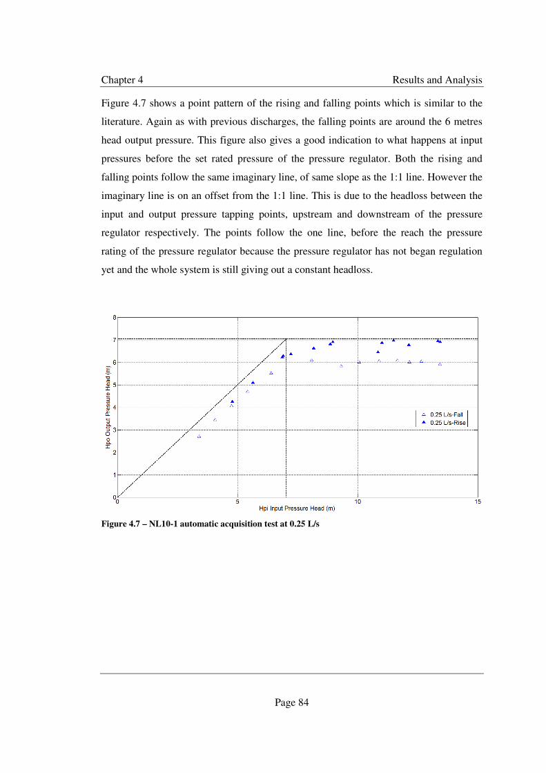
Chapter 4 Results and Analysis
Page 84
Figure 4.7 shows a point pattern of the rising and falling points which is similar to the
literature. Again as with previous discharges, the falling points are around the 6 metres
head output pressure. This figure also gives a good indication to what happens at input
pressures before the set rated pressure of the pressure regulator. Both the rising and
falling points follow the same imaginary line, of same slope as the 1:1 line. However the
imaginary line is on an offset from the 1:1 line. This is due to the headloss between the
input and output pressure tapping points, upstream and downstream of the pressure
regulator respectively. The points follow the one line, before the reach the pressure
rating of the pressure regulator because the pressure regulator has not began regulation
yet and the whole system is still giving out a constant headloss.
Figure 4.7 – NL10-1 automatic acquisition test at 0.25 L/s

Chapter 4 Results and Analysis
Page 85
Figure 4.8– NL10-1 automatic acquisition test at 0.30 L/s
Figure 4.8 like figure Figure 4.7shows a good point pattern, with both the rising and
falling points below the pressure regulators set pressure value following an imaginary
constant sloped line, before the variable regulation kicks in and the rising points separate
from the falling points.
Figure 4.9– NL10-1 automatic acquisition test at 0.50 L/s
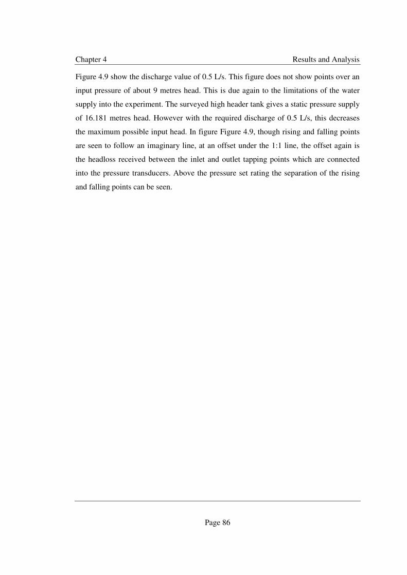
Chapter 4 Results and Analysis
Page 86
Figure 4.9 show the discharge value of 0.5 L/s. This figure does not show points over an
input pressure of about 9 metres head. This is due again to the limitations of the water
supply into the experiment. The surveyed high header tank gives a static pressure supply
of 16.181 metres head. However with the required discharge of 0.5 L/s, this decreases
the maximum possible input head. In figure Figure 4.9, though rising and falling points
are seen to follow an imaginary line, at an offset under the 1:1 line, the offset again is
the headloss received between the inlet and outlet tapping points which are connected
into the pressure transducers. Above the pressure set rating the separation of the rising
and falling points can be seen.
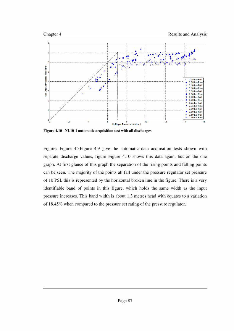
Chapter 4 Results and Analysis
Page 87
Figure 4.10– NL10-1 automatic acquisition test with all discharges
Figures Figure 4.3Figure 4.9 give the automatic data acquisition tests shown with
separate discharge values, figure Figure 4.10 shows this data again, but on the one
graph. At first glance of this graph the separation of the rising points and falling points
can be seen. The majority of the points all fall under the pressure regulator set pressure
of 10 PSI, this is represented by the horizontal broken line in the figure. There is a very
identifiable band of points in this figure, which holds the same width as the input
pressure increases. This band width is about 1.3 metres head with equates to a variation
of 18.45% when compared to the pressure set rating of the pressure regulator.

Chapter 4 Results and Analysis
Page 88
Figure 4.11– NL10-1 automatic acquisition test showing discharge distribution
To compare the output pressure and discharges, figure Figure 4.10 is reproduced with
the discharge in the z axis, figure Figure 4.11 shows this distribution. This figure shows
that each point was plotted with a constant discharge, with a different input and output
pressure. A general trend can also be seen that with an increasing discharge the
maximum output pressure decreased.
4.4 Automatic data acquisition with higher input heads
The automation testing with their figures shown above used the supply for the
experiment from the high header tank which had a surveyed constant water supply level
of 16.181 metres. This gave maximum input pressures of around 150 kPa when losses
are taken into consideration.
Analysis of the results from the automation testing showed that at high discharges
obtained singular points at increased input pressures was not possible. This is due to the
required movement of the valves to get the correct discharge value. However at this
position of the valves the pressure is too low. To overcome this higher input pressure
into the supply of the experiment is needed, for this a pump is included.

Chapter 4 Results and Analysis
Page 89
Figure 4.12 – NL10-1 automatic acquisition test with increased Hpi at 0.2 L/s
Figure 4.12 shows the first figure for automatic data acquisition tests with increased
input head. Like with the stage two tests the rising and falling points are differentiated.
The horizontal broken line represents the set regulation pressure of the pressure
regulator and the vertical broken line also representing the set regulation pressure but on
the x axis. The diagonal line is a 1:1 line from the origin to the interception of these
lines. The figure shows most of the rising output pressure points to be above the
horizontal broken line, which is the pressure regulators set constant output pressure. All
of the falling points are positioned below this line and there does seem that is scatter
amongst the falling points. All the points on this figure are for a constant discharge of
0.2 L/s.
Figure 4.13 shows the figure for the automatic data acquisition test with higher input
pressures for a constant discharge of 0.3 L/s. Like figureFigure 4.12 the rising pressure
points are generally positioned just above the pressure regulators set constant output
pressure. The falling points have more scatter the deviate about 1 metre output pressure
head.

Chapter 4 Results and Analysis
Page 90
Figure 4.13 – NL10-1 automatic acquisition test with increased Hpi at 0.3 L/s
Figure 4.14 shows the graph for a constant discharge of 0.4 L/s. This is the first graph of
this stage of testing where points are shown on the offset from the 1:1 line leading up to
regulation. This figure reports about the same amount of deviation of scatter for both the
rising and falling points of about 0.5 and 0.9 metres head respectively.
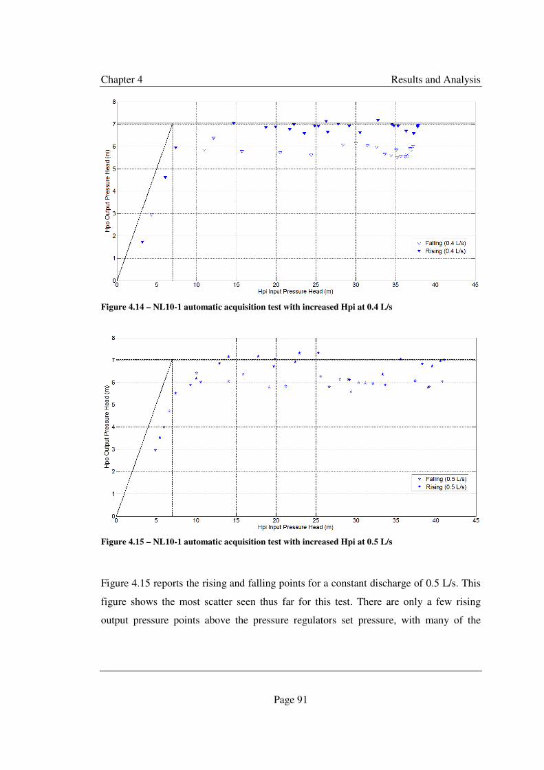
Chapter 4 Results and Analysis
Page 91
Figure 4.14 – NL10-1 automatic acquisition test with increased Hpi at 0.4 L/s
Figure 4.15 – NL10-1 automatic acquisition test with increased Hpi at 0.5 L/s
Figure 4.15 reports the rising and falling points for a constant discharge of 0.5 L/s. This
figure shows the most scatter seen thus far for this test. There are only a few rising
output pressure points above the pressure regulators set pressure, with many of the
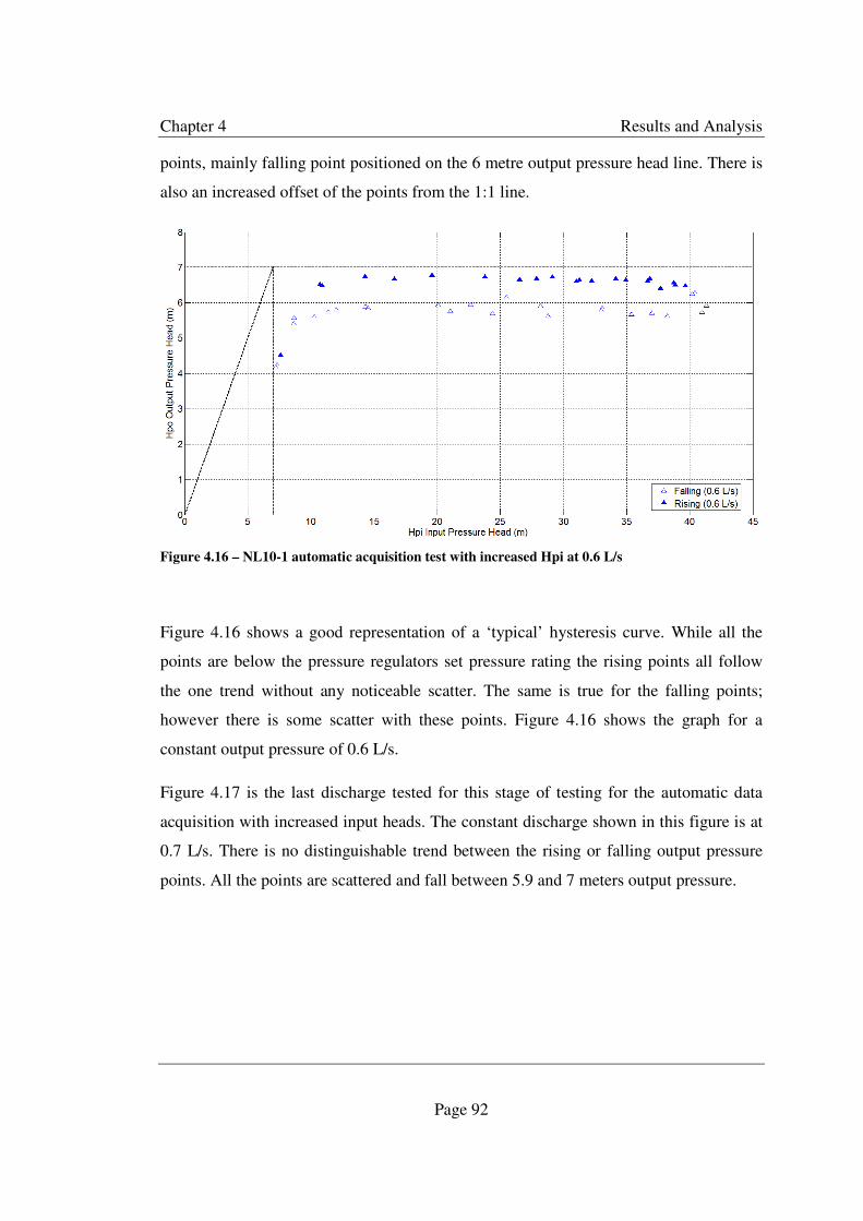
Chapter 4 Results and Analysis
Page 92
points, mainly falling point positioned on the 6 metre output pressure head line. There is
also an increased offset of the points from the 1:1 line.
Figure 4.16 – NL10-1 automatic acquisition test with increased Hpi at 0.6 L/s
Figure 4.16 shows a good representation of a ‘typical’ hysteresis curve. While all the
points are below the pressure regulators set pressure rating the rising points all follow
the one trend without any noticeable scatter. The same is true for the falling points;
however there is some scatter with these points. Figure 4.16 shows the graph for a
constant output pressure of 0.6 L/s.
Figure 4.17 is the last discharge tested for this stage of testing for the automatic data
acquisition with increased input heads. The constant discharge shown in this figure is at
0.7 L/s. There is no distinguishable trend between the rising or falling output pressure
points. All the points are scattered and fall between 5.9 and 7 meters output pressure.

Chapter 4 Results and Analysis
Page 93
Figure 4.17 – NL10-1 automatic acquisition test with increased Hpi at 0.7 L/s
Figure 4.18 – NL10- automatic acquisition test with increased Hpi at all discharges
Figure 4.18 shows all the discharges for this stage of testing; this graph needs to be
interpreted carefully as there is a lot of information portrayed on this graph. At higher
input pressures there seems to be a higher variation of output pressure points. From
inspection of the graph there also seems to be about a third of the rising pressure points
above the pressure regulators set pressure rating.
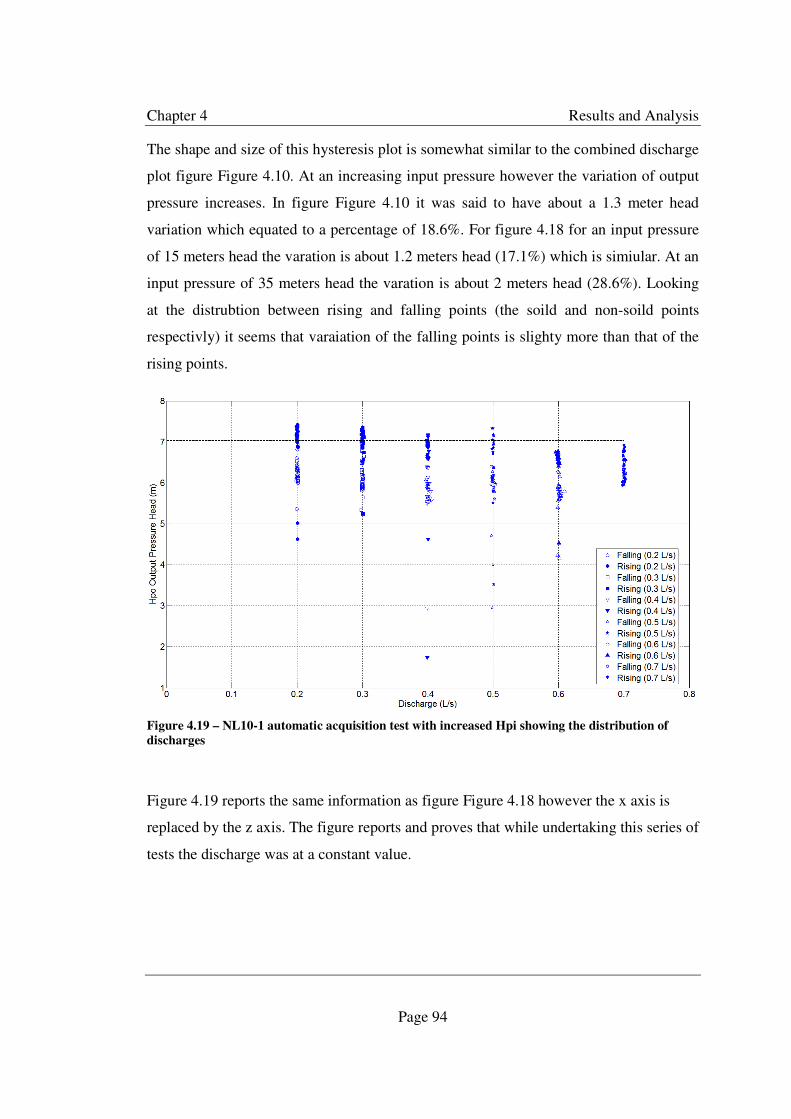
Chapter 4 Results and Analysis
Page 94
The shape and size of this hysteresis plot is somewhat similar to the combined discharge
plot figure Figure 4.10. At an increasing input pressure however the variation of output
pressure increases. In figure Figure 4.10 it was said to have about a 1.3 meter head
variation which equated to a percentage of 18.6%. For figure 4.18 for an input pressure
of 15 meters head the varation is about 1.2 meters head (17.1%) which is simiular. At an
input pressure of 35 meters head the varation is about 2 meters head (28.6%). Looking
at the distrubtion between rising and falling points (the soild and non-soild points
respectivly) it seems that varaiation of the falling points is slighty more than that of the
rising points.
Figure 4.19 – NL10-1 automatic acquisition test with increased Hpi showing the distribution of
discharges
Figure 4.19 reports the same information as figure Figure 4.18 however the x axis is
replaced by the z axis. The figure reports and proves that while undertaking this series of
tests the discharge was at a constant value.
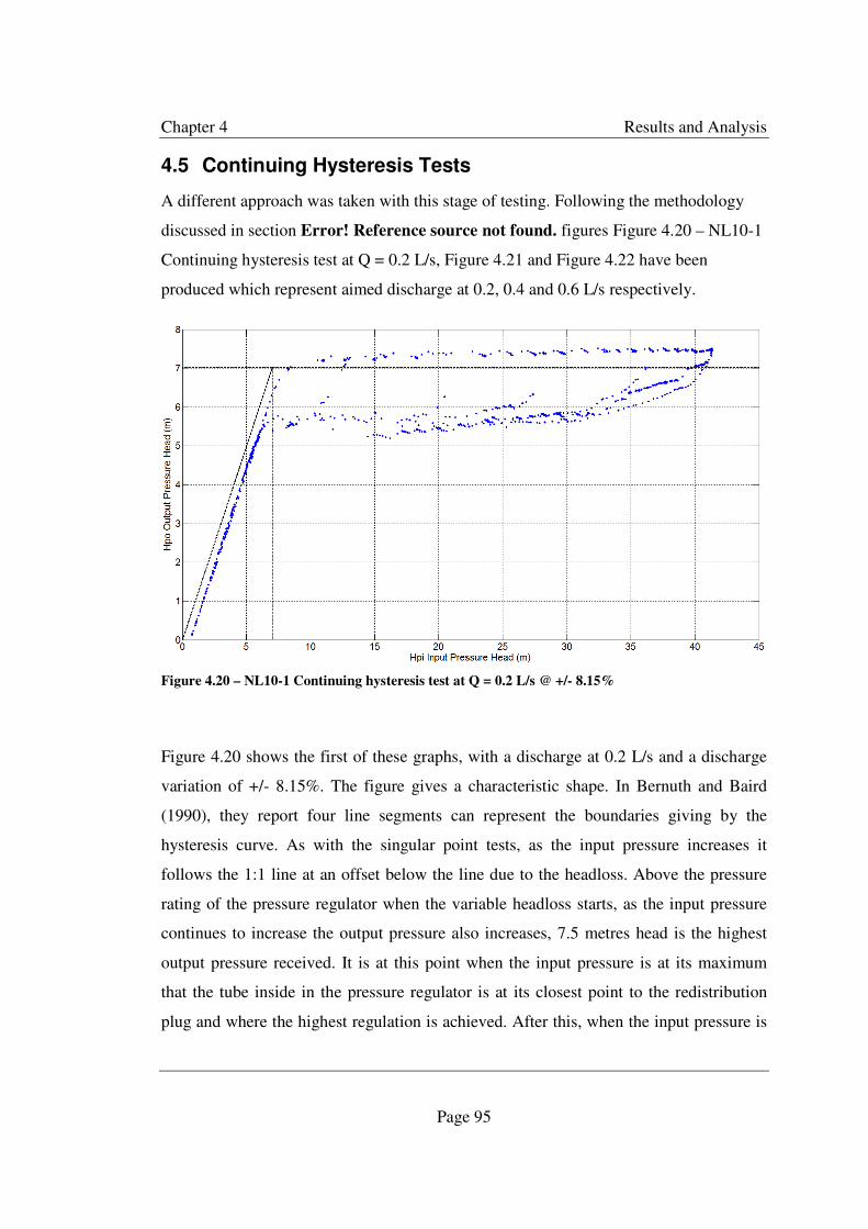
Chapter 4 Results and Analysis
Page 95
4.5 Continuing Hysteresis Tests
A different approach was taken with this stage of testing. Following the methodology
discussed in section Error! Reference source not found. figures Figure 4.20 – NL10-1
Continuing hysteresis test at Q = 0.2 L/s, Figure 4.21 and Figure 4.22 have been
produced which represent aimed discharge at 0.2, 0.4 and 0.6 L/s respectively.
Figure 4.20 – NL10-1 Continuing hysteresis test at Q = 0.2 L/s @ +/- 8.15%
Figure 4.20 shows the first of these graphs, with a discharge at 0.2 L/s and a discharge
variation of +/- 8.15%. The figure gives a characteristic shape. In Bernuth and Baird
(1990), they report four line segments can represent the boundaries giving by the
hysteresis curve. As with the singular point tests, as the input pressure increases it
follows the 1:1 line at an offset below the line due to the headloss. Above the pressure
rating of the pressure regulator when the variable headloss starts, as the input pressure
continues to increase the output pressure also increases, 7.5 metres head is the highest
output pressure received. It is at this point when the input pressure is at its maximum
that the tube inside in the pressure regulator is at its closest point to the redistribution
plug and where the highest regulation is achieved. After this, when the input pressure is
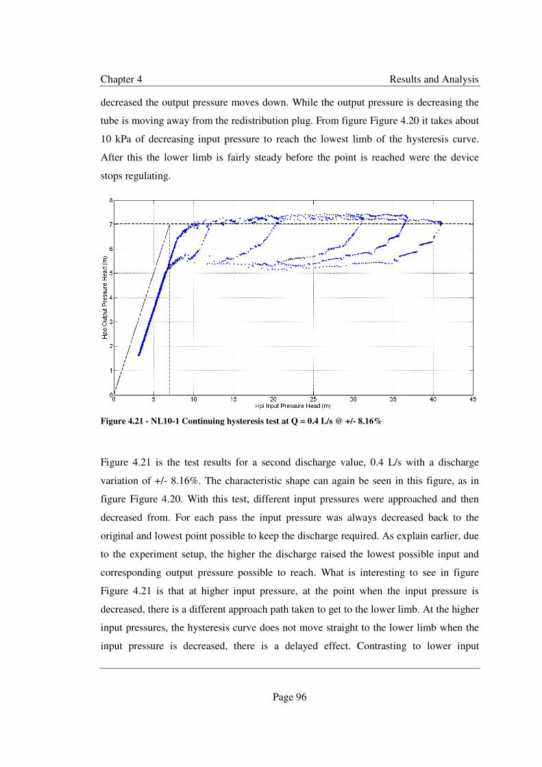
Chapter 4 Results and Analysis
Page 96
decreased the output pressure moves down. While the output pressure is decreasing the
tube is moving away from the redistribution plug. From figure Figure 4.20 it takes about
10 kPa of decreasing input pressure to reach the lowest limb of the hysteresis curve.
After this the lower limb is fairly steady before the point is reached were the device
stops regulating.
Figure 4.21 - NL10-1 Continuing hysteresis test at Q = 0.4 L/s @ +/- 8.16%
Figure 4.21 is the test results for a second discharge value, 0.4 L/s with a discharge
variation of +/- 8.16%. The characteristic shape can again be seen in this figure, as in
figure Figure 4.20. With this test, different input pressures were approached and then
decreased from. For each pass the input pressure was always decreased back to the
original and lowest point possible to keep the discharge required. As explain earlier, due
to the experiment setup, the higher the discharge raised the lowest possible input and
corresponding output pressure possible to reach. What is interesting to see in figure
Figure 4.21 is that at higher input pressure, at the point when the input pressure is
decreased, there is a different approach path taken to get to the lower limb. At the higher
input pressures, the hysteresis curve does not move straight to the lower limb when the
input pressure is decreased, there is a delayed effect. Contrasting to lower input
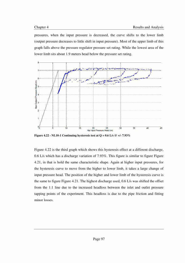
Chapter 4 Results and Analysis
Page 97
pressures, when the input pressure is decreased, the curve shifts to the lower limb
(output pressure decreases to little shift in input pressure). Most of the upper limb of this
graph falls above the pressure regulator pressure set rating. While the lowest area of the
lower limb sits about 1.9 meters head below the pressure set rating.
Figure 4.22 - NL10-1 Continuing hysteresis test at Q = 0.6 L/s @ +/- 7.93%
Figure 4.22 is the third graph which shows this hysteresis effect at a different discharge,
0.6 L/s which has a discharge variation of 7.93%. This figure is similar to figure Figure
4.21, in that is hold the same characteristic shape. Again at higher input pressures, for
the hysteresis curve to move from the higher to lower limb, it takes a large change of
input pressure head. The position of the higher and lower limb of the hysteresis curve is
the same to figure Figure 4.21. The highest discharge used, 0.6 L/s was shifted the offset
from the 1:1 line due to the increased headloss between the inlet and outlet pressure
tapping points of the experiment. This headloss is due to the pipe friction and fitting
minor losses.
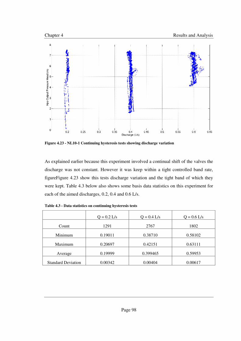
Chapter 4 Results and Analysis
Page 98
Figure 4.23 - NL10-1 Continuing hysteresis tests showing discharge variation
As explained earlier because this experiment involved a continual shift of the valves the
discharge was not constant. However it was keep within a tight controlled band rate,
figureFigure 4.23 show this tests discharge variation and the tight band of which they
were kept. Table 4.3 below also shows some basis data statistics on this experiment for
each of the aimed discharges, 0.2, 0.4 and 0.6 L/s.
Table 4.3 - Data statistics on continuing hysteresis tests
Q = 0.2 L/s Q = 0.4 L/s Q = 0.6 L/s
Count 1291 2767 1802
Minimum 0.19011 0.38710 0.58102
Maximum 0.20697 0.42151 0.63111
Average 0.19999 0.399465 0.59953
Standard Deviation 0.00342 0.00404 0.00617

Chapter 4 Results and Analysis
Page 99
4.6 Creep Test
Section 3.7 outlines the methodology undertaken for this stage of tests. The creep tests
investigates the movement of tube and thus the shift of regulation of the pressure
regulator when in operation for a long period of time.
Figure 4.24 – Rising pressure 24 hour creep test
Figure 4.24 – Rising pressure 24 hour creep test shows a graph for this creep tests for a
rising output pressure. The test was run for a 24 hour period and each point of data
represents one second of this period of time. Similarly figureFigure 4.25 – Falling
pressure 24 hour creep testshows the graph for a falling output pressure. This test was
run straight after the test of the rising pressures and it was run for the same amount of
time, 24 hours.
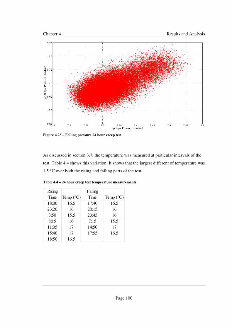
Chapter 4 Results and Analysis
Page 100
Figure 4.25 – Falling pressure 24 hour creep test
As discussed in section 3.7, the temperature was measured at particular intervals of the
test. Table 4.4 shows this variation. It shows that the largest different of temperature was
1.5 °C over both the rising and falling parts of the test.
Table 4.4 – 24 hour creep test temperature measurements
Rising Falling
Time Temp (°C) Time Temp (°C)
18:00 16.5 17:40 16.5
23:20 16 20:15 16
3:50 15.5 23:45 16
8:15 16 7:15 15.5
11:05 17 14:50 17
15:40 17 17:55 16.5
18:50 16.5

Chapter 4 Results and Analysis
Page 101
Table 4.5 – Creep test minimum, maximum and variation values.
Minimum Maximum Variation (%)
Rising Input Pressure 13.045 13.256 1.59
Rising Output Pressure 6.7388 6.9701 3.31
Falling Input Pressure 7.1783 7.5981 5.52
Falling Output Pressure 5.5665 5.8452 4.76
Following on from the temperature variation, the variation in the graphs are analysed.
Table 4.5 reports these variations of the input and output pressures for both the rising
and falling tests. It shows that move variation is reported with the falling test, than the
rising tests.
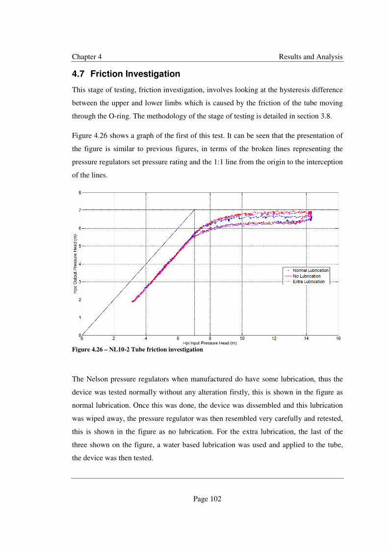
Chapter 4 Results and Analysis
Page 102
4.7 Friction Investigation
This stage of testing, friction investigation, involves looking at the hysteresis difference
between the upper and lower limbs which is caused by the friction of the tube moving
through the O-ring. The methodology of the stage of testing is detailed in section 3.8.
Figure 4.26 shows a graph of the first of this test. It can be seen that the presentation of
the figure is similar to previous figures, in terms of the broken lines representing the
pressure regulators set pressure rating and the 1:1 line from the origin to the interception
of the lines.
Figure 4.26 – NL10-2 Tube friction investigation
The Nelson pressure regulators when manufactured do have some lubrication, thus the
device was tested normally without any alteration firstly, this is shown in the figure as
normal lubrication. Once this was done, the device was dissembled and this lubrication
was wiped away, the pressure regulator was then resembled very carefully and retested,
this is shown in the figure as no lubrication. For the extra lubrication, the last of the
three shown on the figure, a water based lubrication was used and applied to the tube,
the device was then tested.

Chapter 4 Results and Analysis
Page 103
All three tests fit together as they approach regulation, under the 1:1 line. As the upper
limb of the graph is approached the three tests separate out. While no points go above
the pressure regulators set pressure rating the extra lubrication test is the closest to this
line. Just underneath the extra lubrication test is the no lubrication test. The upper limb
of the normal test is below the no lubrication. On the lower limb, all three tests follow
the same path back to the constant approach line. Like with previous tests an
understanding of the discharge variation is important and is shown for this test in
figureFigure 4.27. This point plot shows all the discharges for the three tests. From this
plot a 6.6% variation of discharge is shown.
Figure 4.27 – NL10-2 Tube friction investigation showing discharge variation

Chapter 4 Results and Analysis
Page 104
Figure 4.28 – NL10-3 Tube friction investigation
Figure 4.28 shows the second plot for the friction investigation. For this test extra input
head was used. The upper limb of this graph shows the normal and extra lubrication to
be at about the same output pressure, following the pressure regulators pressure set line
for the increase input pressure. The no lubrication for the upper limb is above the
pressure set line at about 0.2 metres output head. Like with the continuing hysteresis test
different input pressures where the experiment shifted from rising to falling pressures.
On the lower limb the normal lubrication test has the lowest output pressure. The extra
and no lubrication tests follow the same path however at the lower input pressures the
extra lubrication output pressure raises slightly. The test with the smallest distance
between the upper and lower limbs is the extra lubrication test. Figure 4.29 shows the
discharge variation for the three tests, normal, no and extra lubrication. The aimed
discharge for this test was 0.3 L/s and the variation was 14.2%.
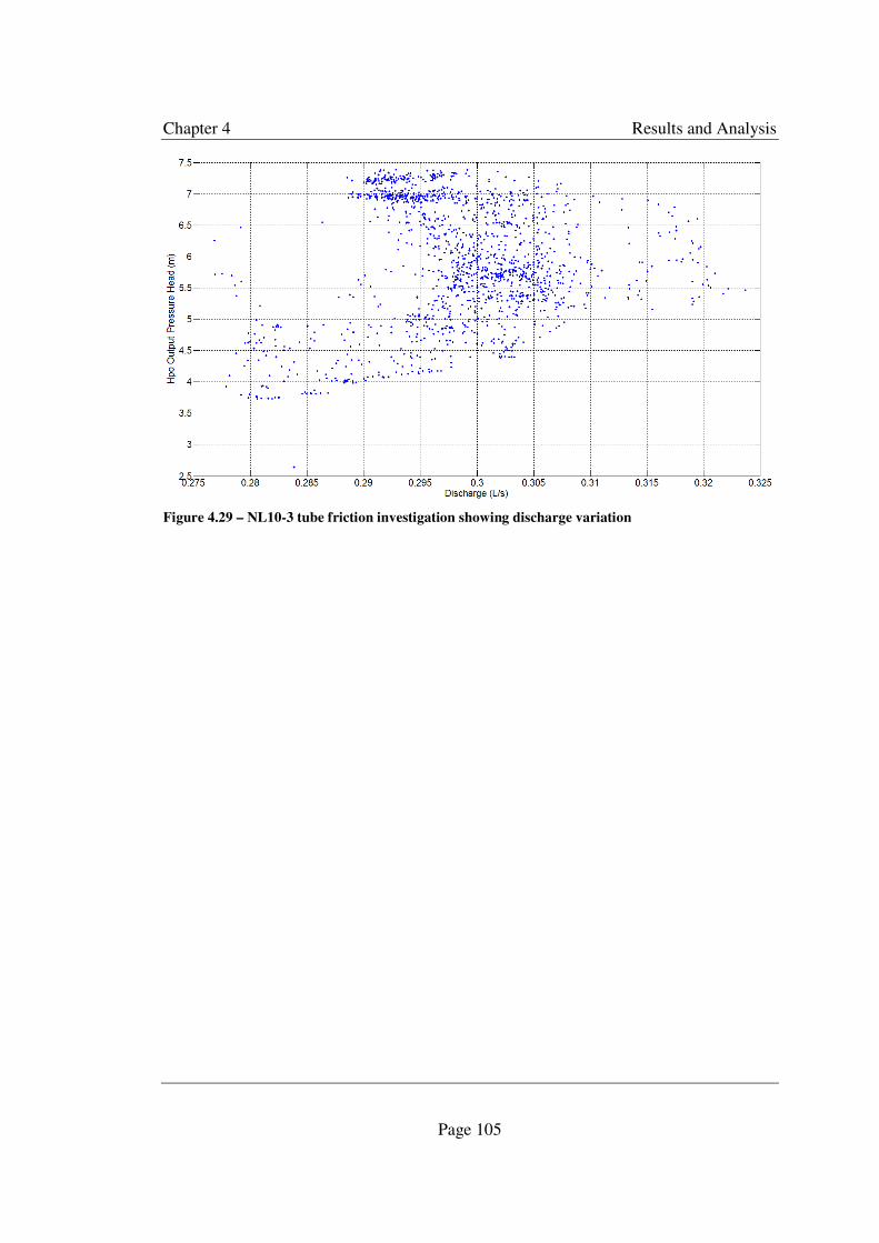
Chapter 4 Results and Analysis
Page 105
Figure 4.29 – NL10-3 tube friction investigation showing discharge variation
Chapter 4
4.8 Movement of Tube inside Pressure Regulator
The regulation part of the pressure regulator is controlled by the tubes displacement.
This stage of tests was investigated to study this displacement and the rate of
displacement of the tube inside the pressure regulator. Section
not found. explains how the materials were used for this experiment and the
methodology undertaken.
Figure 4.30 – NL10-TD Tube up
Figure 4.30 shows the first of the graphs for this stage of testing. The graph sh
parameters. The input and output pressure are displayed and read from the secondary y
axis, on the right hand side of the graph. Both the input and output pressures units are in
metres head. The discharge is displayed on the primary y axis along w
distance.
Page 106
Movement of Tube inside Pressure Regulator
The regulation part of the pressure regulator is controlled by the tubes displacement.
This stage of tests was investigated to study this displacement and the rate of
displacement of the tube inside the pressure regulator. Section Error! Reference source
explains how the materials were used for this experiment and the
methodology undertaken.
TD Tube upward displacement investigation with 3TN #15 nozzle
shows the first of the graphs for this stage of testing. The graph sh
parameters. The input and output pressure are displayed and read from the secondary y
axis, on the right hand side of the graph. Both the input and output pressures units are in
metres head. The discharge is displayed on the primary y axis along w
Results and Analysis
Movement of Tube inside Pressure Regulator
The regulation part of the pressure regulator is controlled by the tubes displacement.
This stage of tests was investigated to study this displacement and the rate of
Error! Reference source
explains how the materials were used for this experiment and the
ward displacement investigation with 3TN #15 nozzle
shows the first of the graphs for this stage of testing. The graph shows four
parameters. The input and output pressure are displayed and read from the secondary y
axis, on the right hand side of the graph. Both the input and output pressures units are in
metres head. The discharge is displayed on the primary y axis along with the opening
Chapter 4 Results and Analysis
Page 107
The opening distance is the distance between the tube and the lip on the redistribution
plug. Appendix B shows a schematic diagram of the pressure regulator which shows this
distance. This distance by the circumference around the tube is the area which the fluid
is allowed to enter into the tube for its regulation and where the variable headloss
occurs. The x axis on figure Figure 4.30 shows the time which test was carried out for.
The discharge shows an exponential increase as the valve is turned on, this is what is
expected to be seen for the discharge. For the discharge to be included on the figure the
display is very small as the experimental setup restricted large discharges to be tested. A
3TN #15 nozzle was used for this test, replicating a small discharge.
As the valve was turned on and the input pressure increased, figure Figure 4.30 shows
the time taken to get to full pressure to be about 8-10 seconds. It is expected once the
input pressure was above the pressure regulators set output pressure the regulation
would begin and the output pressure would level out. However the output pressure was
seen to increase at a fairly steady and constant rate until the test stopped, it finished at
about 7.2 metres head.
At the start of this test the tube was in its furthest position from the lip of the
redistribution plug of 4.7 mm. The tubes displacement was measured which moved
closer to this lip and finished at 3.066 mm from the lip. The tube move towards the lip
1.634 mm. The rate of this displacement also is important. With reference to figure
Figure 4.30 the tube as moved back slightly, which means the spring has had a force
causing it to displace the tube. The tube then does not move from this position before it
suddenly moves forward, which is where most of the displacement occurs. For another
minute of testing, the tube continues to move forward at different increments before the
end of the test. The sudden movement forward of the tube occurs when the input
pressure is increased the most, which what would be expected to be seen.

Chapter 4
Figure 4.31 - NL10-TD Tube down
Figure 4.31 shows a graph for the closing of the valve with the same nozzle, 3TN #15.
The same presentation of the graph is seen as figure
the secondary y axis and the opening distance and discharge displayed on the primary y
axis. Time is on the x axis.
This test starts with the valve fully on and the discharge at its maximum point. As the
tests is continued and the valve tur
the valve is fully turned on the pressure regulator is regulating the pressure, this is seen
as the output pressure stays constant. However when the input pressure is decreasing
and above the pressure reg
to decrease slightly.
The tubes movement for this test
incremental movements, the major movement away from the lip was at the point when
the valve was about 90% shut and the input and output pressure dropped. The tube then
displaced back to its origin of 4.7 mm away from the lip.
Page 108
TD Tube downward displacement investigation with 3TN #15 nozzle
shows a graph for the closing of the valve with the same nozzle, 3TN #15.
The same presentation of the graph is seen as figure Figure 4.30, with t
the secondary y axis and the opening distance and discharge displayed on the primary y
on the x axis.
This test starts with the valve fully on and the discharge at its maximum point. As the
tests is continued and the valve turned off, the discharge is exponential decreased. As
the valve is fully turned on the pressure regulator is regulating the pressure, this is seen
as the output pressure stays constant. However when the input pressure is decreasing
and above the pressure regulators set constant output pressure the output pressure is seen
The tubes movement for this test saw no major change, apart from a few small
incremental movements, the major movement away from the lip was at the point when
was about 90% shut and the input and output pressure dropped. The tube then
displaced back to its origin of 4.7 mm away from the lip.
Results and Analysis
ward displacement investigation with 3TN #15 nozzle
shows a graph for the closing of the valve with the same nozzle, 3TN #15.
, with the pressures on
the secondary y axis and the opening distance and discharge displayed on the primary y
This test starts with the valve fully on and the discharge at its maximum point. As the
ned off, the discharge is exponential decreased. As
the valve is fully turned on the pressure regulator is regulating the pressure, this is seen
as the output pressure stays constant. However when the input pressure is decreasing
ulators set constant output pressure the output pressure is seen
saw no major change, apart from a few small
incremental movements, the major movement away from the lip was at the point when
was about 90% shut and the input and output pressure dropped. The tube then

Chapter 4
Figure 4.32 - NL10-TD Tube upward displacement investigation with 3TN
Figure 4.32 shows the first of the second part for this test using a larger sized nozzle.
Due to the limitations of the testing rig a medium sized nozzle was used which gave a
maximum discharge of 0.28 L/s. In this figure, with the valve fully shut and opened
slowly the discharge is seen to have a more
on. The pressure difference between the input and output pressures are more to be
expected in figure Figure
rising, the difference between the lines is increasing, this is due to the increased velocity
and the increased headloss between the input and output fittings. The output pressu
then levels off at the regulation pressure, while the input pressure continues to increase.
Again however the output pressure getting to regulating is gradual and it is not as quick
as expected.
The tubes movement again begins by slightly moving backwar
nearly 2 minutes into the test the tube takes a few incremental steps forward. There is a
small sudden movement forward before the
Page 109
TD Tube upward displacement investigation with 3TN
shows the first of the second part for this test using a larger sized nozzle.
Due to the limitations of the testing rig a medium sized nozzle was used which gave a
maximum discharge of 0.28 L/s. In this figure, with the valve fully shut and opened
the discharge is seen to have a more characteristic curve as the valve is turned
The pressure difference between the input and output pressures are more to be
Figure 4.32. On the approach with the input and output pressure
rising, the difference between the lines is increasing, this is due to the increased velocity
and the increased headloss between the input and output fittings. The output pressu
then levels off at the regulation pressure, while the input pressure continues to increase.
Again however the output pressure getting to regulating is gradual and it is not as quick
The tubes movement again begins by slightly moving backward away from the lip. At
nearly 2 minutes into the test the tube takes a few incremental steps forward. There is a
small sudden movement forward before the tube stops it movement.
Results and Analysis
#28 nozzle
shows the first of the second part for this test using a larger sized nozzle.
Due to the limitations of the testing rig a medium sized nozzle was used which gave a
maximum discharge of 0.28 L/s. In this figure, with the valve fully shut and opened
curve as the valve is turned
The pressure difference between the input and output pressures are more to be
. On the approach with the input and output pressure
rising, the difference between the lines is increasing, this is due to the increased velocity
and the increased headloss between the input and output fittings. The output pressure
then levels off at the regulation pressure, while the input pressure continues to increase.
Again however the output pressure getting to regulating is gradual and it is not as quick
d away from the lip. At
nearly 2 minutes into the test the tube takes a few incremental steps forward. There is a
tube stops it movement.

Chapter 4
Figure 4.33 - NL10-TD Tube
Figure 4.33 shows the last of the graphs for this test. The tube is displaced down and the
3TN #28 nozzle is used. The exponential shape of the discharge can be seen again. With
the valve fully open and the pressure regulator functioning the large difference between
the input and output pressures can be seen. As the input pressure is decreased, so too
does the output pressure, before it theoretical should
the set rating pressure of the pressure regulator
point the difference closes and the pressure decrease.
seen again as a generalised S
back suddenly and then steadies off. Again the point where the tube moves its most is
when the valve is about 90% shut off and the pressure drop back to zero.
Page 110
TD Tube downward displacement investigation with 3TN #28 nozzle
shows the last of the graphs for this test. The tube is displaced down and the
used. The exponential shape of the discharge can be seen again. With
the valve fully open and the pressure regulator functioning the large difference between
the input and output pressures can be seen. As the input pressure is decreased, so too
tput pressure, before it theoretical should, as the input pressure is still above
the set rating pressure of the pressure regulator. When the input pressure does get to this
point the difference closes and the pressure decrease. The displacement of the tub
seen again as a generalised S-curve; where it slowly moves back from the lip, shifts
back suddenly and then steadies off. Again the point where the tube moves its most is
when the valve is about 90% shut off and the pressure drop back to zero.
Results and Analysis
downward displacement investigation with 3TN #28 nozzle
shows the last of the graphs for this test. The tube is displaced down and the
used. The exponential shape of the discharge can be seen again. With
the valve fully open and the pressure regulator functioning the large difference between
the input and output pressures can be seen. As the input pressure is decreased, so too
, as the input pressure is still above
When the input pressure does get to this
The displacement of the tube is
curve; where it slowly moves back from the lip, shifts
back suddenly and then steadies off. Again the point where the tube moves its most is
when the valve is about 90% shut off and the pressure drop back to zero.
Chapter 4 Results and Analysis
Page 111
4.9 Statistical Analysis
4.9.1 Introduction
Following variation differences seen in the performance of the pressure regulator. A
statistical analysis is performed to understand the variation and to also calculate to
sample size of pressure regulators which are needed to adequately characterise
manufacturers’ variation in their manufacturing of pressure regulators. Section 4.9
outlines the methodology which has been used for this statistical analysis. An ANOVA
(analysis of variation) has been performed for two discharges. The normal model theory
has been applied to calculate the sample size of the number of pressure regulators which
need to be tested.
4.9.2 The ANOVA test
Nelson Nozzle 3TN #28
The null hypotheses is stated the all the means of the five tests of each pressure regulator
are equal.
RS : K4 = K5 = KU 4.1
The treatment sum of squares is calculated;
WWX� = #4�x4̄ − x̄�5 + #5�x5̄ − x̄�5 + ⋯ + #]�xk̄ − x̄�5 4.2
The number of tests for each pressure regulator was 5, thus nk = 5, x̄ is the pressure
regulators set pressure rating in metres head = 7.04321, x4̄ is the mean of the 5 tests for
each pressure regulator.
WWX� = 1.0375 4.3
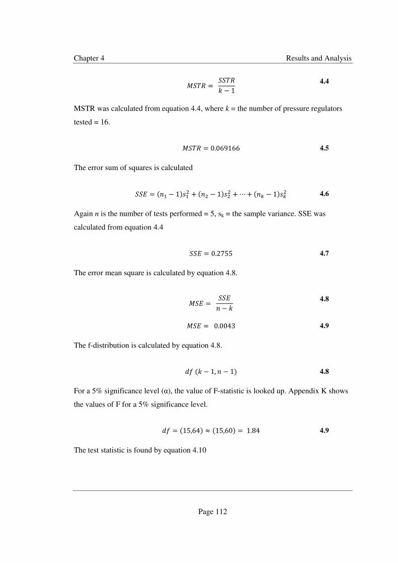
Chapter 4 Results and Analysis
Page 112
*WX� = WWX�Y − 1
4.4
MSTR was calculated from equation 4.4, where k = the number of pressure regulators
tested = 16.
*WX� = 0.069166 4.5
The error sum of squares is calculated
WW� = �#4 − 1��45 + �#5 − 1��55 + ⋯ + �#] − 1��]5 4.6
Again n is the number of tests performed = 5, sk = the sample variance. SSE was
calculated from equation 4.4
WW� = 0.2755 4.7
The error mean square is calculated by equation 4.8.
*W� = WW�# − Y
4.8
*W� = 0.0043 4.9
The f-distribution is calculated by equation 4.8.
�� �Y − 1, # − 1� 4.8
For a 5% significance level (α), the value of F-statistic is looked up. Appendix K shows
the values of F for a 5% significance level.
�� = �15,64� ≈ �15,60� = 1.84 4.9
The test statistic is found by equation 4.10
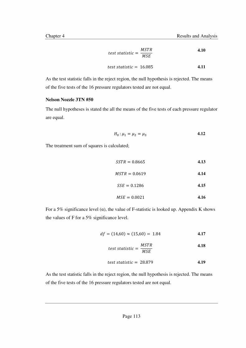
Chapter 4 Results and Analysis
Page 113
� �� ��������E = *WX�*W�
4.10
� �� ��������E = 16.085 4.11
As the test statistic falls in the reject region, the null hypothesis is rejected. The means
of the five tests of the 16 pressure regulators tested are not equal.
Nelson Nozzle 3TN #50
The null hypotheses is stated the all the means of the five tests of each pressure regulator
are equal.
RS : K4 = K5 = KU 4.12
The treatment sum of squares is calculated;
WWX� = 0.8665 4.13
*WX� = 0.0619 4.14
WW� = 0.1286 4.15
*W� = 0.0021 4.16
For a 5% significance level (α), the value of F-statistic is looked up. Appendix K shows
the values of F for a 5% significance level.
�� = �14,60� ≈ �15,60� = 1.84 4.17
� �� ��������E = *WX�*W�
4.18
� �� ��������E = 28.879 4.19
As the test statistic falls in the reject region, the null hypothesis is rejected. The means
of the five tests of the 16 pressure regulators tested are not equal.

Chapter 4 Results and Analysis
Page 114
4.9.3 Determination of Sample Size
The normal model was used to calculate the sample size for the number of pressure
regulators which needed to be tested. Equation 4.20 was used for this process.
# = � 'ȳO P
Q�5 4.20
where σ is the standard deviation, ȳ is the theoretical mean, µ is the mean, z is the z-
score and n is the sample size.
Nelson Nozzle 3TN #28
# = � 0.1288m.SnU54O m.S4i4m
4.oi�5 = 87.16 = 88
4.21
88 pressure regulators are needed to be tested, as 16 devices have already been tested,
72 more tests need to be carried out.
Nelson Nozzle 3TN #50
# = � 0.1065m.SnU54O p.5Sip
4.oi�5 = 0.0129 = 1
4.22
From the calculation is equation 4.22 the number of devices needed to be tested is
rounded up to 1. This calculation is unreasonable; this is due to the mean of the tests
carried out. At the higher discharge the output pressure is lower and the difference
between the pressure regulators set pressure rating and the mean of the tests of the 16
Nelson pressure regulators is large due to the higher discharge, from a larger nozzle size
used.
Chapter 5 Discussion
Page 115
Chapter 5 DISCUSSION
5.1 Introduction
This chapter provides a discussion on the results and analysis provided in the previous
chapter. Each series of tests will be discussed, the first being the tests set out to replicate
the results from the literature.
5.2 Result Replication from von Bernuth and Baird (1990)
The first stages of testing were to try and replicate the results from von Bernuth and
Baird (1990). In replicating the results from this literature a similar test rig was
constructed, however they were some major differences. To obtain a constant discharge
for the test Bernuth and Baird used a discharge controlled regulator (with a set pressure
of 68.9 kPa) and a precision orifice. This discharge control regulator was a previously
tested pressure regulator. Figure 2.2 shows the schematic used by von Bernuth and
Baird (1990).
The test rig which was constructed to replicate the results, consisted of valves placed
both sides of the pressure regulator being tested and each one manipulated, a nozzle was
used to control the discharge from the experiment. Two pressure regulators were used in
this manual test. The first was a Valley 6 PSI pressure set pressure regulator with a ¾
female to ¾ female connection fitting and the second was a Nelson 10 PSI pressure set
pressure regulator with a ¾ female to ¾ female connection fittings.
This early testing in replicating the results from von Bernuth and Baird (1990) clearly
established the importance of using the upstream and downstream valves and how their
use, influenced the discharge and input and output pressure in the testing rig. Table 4.1
shows this influence. In contrast to von Bernuth and Baird (1990) testing rig, where one
valve was used and a second discharge controlled regulator was used. There is no real
discharge control with their experimental methodology. To obtain multiple points
around the hysteresis curve for stage one testing is time consuming because of the slight
movement of the valves required to achieve a constant discharge. Levers were

Chapter 5 Discussion
Page 116
connected to these valves; however they were short levers which had limited control
over the valves.
From the result replication test from von Bernuth and Baird it was thought to keep the
same hydraulic setup of the testing rig. However better control over the levers was
needed to get to the accuracy of the discharges values. To do this longer extension levers
were designed and made which gave the movement of the valve from a smaller
increment change of the lever.
It was found that many points were needed to get enough data around the hysteresis
curve to understand what was happening. More points were tried to be sourced for
subsequence tests.
5.2.1 Automatic Data Acquisition Test Results
After the literature replication tests were analysed the testrig was further developed to
allow for automation data acquisition. The second major change also was the
introduction of long levers controlling the movement over the two valves. This allowed
getting minute movements of the valves and thus achieving higher precision on the
discharge of the experiment. Seven different discharge values were tested of the one
pressure regulator. A Nelson 10 PSI pressure set pressure regulator, the same device
used in the literature replication tests.
Generally these tests saw the upper and lower bounds of the hysteresis curve. However
there was scatter of the values, particularly with the rising points of the tests. In contrast
it seems that the falling points do not deviate much on the output pressure axis. The
difference between this series of tests and the tests by Bernuth and Baird (1990), there
is not a clear differentiation with this tests, however with Bernuth and Baird (1990)
there is a clear difference, which makes the line fitting to their data and analysis easier.
The water supply for this experiment was from the high header tank which gave much
lower input heads for the different discharges when compared to Bernuth and Baird
(1990). It is believed that due to the force equilibrium in the pressure regulators is why
the scatter is experienced for the rising input pressure. Appendix B shows a schematic

Chapter 5 Discussion
Page 117
diagram for a Nelson 10 PSI pressure regulator, the same one tested for this test,
however appendixAppendix B shows a different connection fitting. When in operation
the force of the spring is pushing the tube down. Counteracting this force is the pressure
of water behind the rubber skirt, which acts as a force up. Together these make up the
two main forces which result in the regulation action of the pressure regulator. When a
rising pressure is being tested, the tube is in a forward movement towards the
redistribution plug, when a falling pressure is being tested the tube is in a backward
movement away from the redistribution plug. There is a third force induced while the
tube is moving, and this is the frictional force when the tube moves through the O-ring.
It is though due to the low input heads which have been tested in this stage of testing,
automatic data acquisition, the force equilibrium which is needed for the tube to be
moved for regulation, particularly the force behind the rubber skirt which is pressurised
by the input pressure is not great enough to overcome the normal forces required and the
frictional force which is why scatter is seen for the rising pressures in the test stage
figures.
For the falling figures because the tube is moving away from the redistribution plug, by
the force of the spring, as the force under the rubber skirt is reduced the falling output
pressure points are generally positioned on the same output pressure.
When pressure regulators are installed on large mobile irrigation machines and in
operation their input pressures are going to much higher, typically in the order of 200 –
400 kPa. Due to this higher input pressures are needed in the experimental testing rig to
understand what these devices do at higher input pressures and what the performance of
their regulation is at these higher input pressures.
5.2.2 Automation Testing with Higher Input Pressures
The same methodology was taken with this stage of testing as with stage previous to
this. It was wanted to saw the effect with high input pressures on the singular point
graph and to see if it followed the same trend as without the introduction of the pump.
To understand the effect the high input pressures would have on the pressure regulators,

Chapter 5 Discussion
Page 118
such as they would be operation on large mobile irrigation machines. Six different
discharges were tested for the automation testing with higher input pressures; these are
0.2 L/s through to 0.7 L/s at 0.1 L/s increments.
It was found with this test that the regulation of the pressure regulator does function at
higher input pressures, the performance of this regulation needs to be looked at. Large
degrees of scatter were found with this test, particularly with the falling output pressure
points. This is conversely different to what was found in the previous stage tests, as the
scatter was generally present for the rising output pressure points. It is believed that this
is again due to the force equilibrium. With the higher input pressures, this gave the
pressure regulator higher forces behind the rubber skirt. These higher forces gave a
better and more defined counteraction on the force induced by the spring; the results
from this moved the tube in a more definitive displacement. This is why the rising points
do not have much scatter in this test, because the higher input pressure induced a large
force which gave a better force equilibrium.
The falling points have more scatter directly for the reason given above, which keep the
rising points from have no scatter. The larger forces behind the rubber skirt do not
resolve completely with the spring to move the tube away from the redistribution plug.
When the frictional force is brought into this equation the scatter is made worse due to
the rubbing of the tube on the O-ring.
What is seen also with this stage of testing is as the discharge increase the rising output
pressures decrease. The same effect can be said for the falling output pressure points,
however the shift is not to the same degree. As the discharge increases then, the
hysteresis pattern migrates downwards.
In figureFigure 4.17 the discharge of 0.7 L/s is reported, the points of this discharge do
not have a distinguishable different between the rising and falling points. The Nelson
manufacturer’s literature on this product report that the flow range for the Nelson 10 PSI
pressure regulator is 0.0315 to 0.6309 L/s. This means that the highest discharge tested
falls outside this range.

Chapter 5 Discussion
Page 119
Bernuth and Baird (1990) did not test high range discharges, so the effect this has on
pressure regulator remains unknown. Australian irrigators have installed large mobile
irrigation machines which have a system capacity to irrigate with higher discharges. A
higher discharge results in the velocity through the pressure regulator being increased.
This speeds up the function of pressure regulator, because the fluid is being passed
through the device at a quicker rate and the pressure response through the device is
quicker because of the increase velocity through the tube.
The water inside the tube when in operation has a friction loss, due to the fluid being
forced against the plastic tube. At a high discharge, the increased velocity creates
another force in the tube. As the water is displaced around the redistribution plug and
into the tube it pulls the tube down, away from the redistribution plug. This force acts in
the same direction as the spring, and in opposite direction to the force under the rubber
skirt and the friction force through the O-ring.
For this test to really be definitive more tests need to be repeated, on this pressure
regulator but also different pressure regulators of the same model and type.
This stage of testing as with the previous stage looked at obtaining multiple rising and
falling output pressure points around the hysteresis curve. Each point was not obtained
in chronological order, thus a stage of testing was looked at where is was true and the
tube was on a continual movement.
5.3 Continuing Hysteresis Tests
These tests saw the first major changes in the way the experiment testrig was used in the
tests. Instead of getting multiple points at a constant discharge, the valves were
continual altered in sequence. Three different discharges were tested these being 0.2, 0.4
and 0.6 L/s. Section Error! Reference source not found. describes the methodology
taken with this test. Section 4.5 presents the figure and analysis the data for the
continuing hysteresis tests.
In interpretation of the results of the hysteresis tests, thought needs to put back to the
physical components of the pressure regulator. The continuing hysteresis tests involved
Chapter 5 Discussion
Page 120
continually moving the valves allowing the input pressure to be increased and
decreased. The effect this has on the pressure regulators is that the tube is moving
towards the redistribution plug and away from the redistribution plug for the regulation
of the input pressure which was continually changing. An increasing input pressure
means that once the pressure gets above the pressure regulators set pressure rating the
device needs to start regulating so the tube moves forwards. The distance it moves and
the rate of movement depends on the nature of the input pressure being fed into the
device. This is due to the pressure behind the tube and counteracting the spring to arrive
at the correct position for the tube to be from the correct pressure regulation.
When this theory is applied back to figuresFigure 4.20, Figure 4.21 and Figure 4.22 and
in their interpretation, we can see this. In figure Figure 4.21 at higher input pressure,
when they are decreased, there are patterns where the tube on its new positioning
downwards is lagged. It will not move or move slightly then suddenly move. At lower
input pressure it seems to move with less resistance. It is believed this is due to the
lower forces acting on the tubes movement at the lower input pressures.
Each test of the different discharges gives a characteristic curve. With mostly all of the
upper limb values above the pressure regulators pressure set rating. This upper limb is
also slightly curved upwards. With the middle valued input pressures giving higher
output pressure then the two lower and higher input pressures which give a
comparatively smaller output pressure. On the lower limb of the hysteresis curve this
effect can also be seen to some extent. Middle input pressure on the lower limb of the
curve give out the lowest output pressure and higher input pressure on the lower limb
give out the higher output pressures. However at about 15 meters head input pressure
the output pressure increases about 0.5 meters head and settles back down to its value
before it spiked. This effect is seen more in figure Figure 4.22 with a discharge of 0.6
L/s, but is also seen in the lower two discharges. The cause of this is due to the tube
suddenly moving while the input pressure is decreased at a constant rate. It is seen more
so at a higher discharge because of the extra volume of water passing though the device
and from this the extra physical forces when the pressure regulator is in operation.

Chapter 5 Discussion
Page 121
The continuing hysteresis tests are different to the singular points tests in such that the
valves were in constant movement. This meant that the discharge could not be recorded
as a constant value, they is variation. Control could however be placed on the amount of
variation of the discharge throughout the test. A narrow band rate was selected and the
discharge was not allowed to go above or below that value. This band rate was selected
to be 10% of the discharge being examined. Figure 4.23 shows this discharge variation
for the continuing hysteresis tests. Table 4.3 - Data statistics on continuing hysteresis
tests also shows some basis data statistics on the discharge variation. For all three tests
discharges the variation is about 8% under the set 10% selected.
5.4 Creep Tests
LMIM when in operation will typically run for hours at a time irrigating the field. When
pressure regulators are installed on LMIM, they too will be in constant operation for
hours at a time. As a development from the singular point tests it was hypothesised that
after long term operation the pressure regulator will shift its tube position which in turn
would move either decrease or increase the output pressure. Both a rising and falling
pressure was considered and tested for 24 hours.
Figure 4.24 displays a point plot of the input and output pressures from the pressure
regulator over the 24 hour period. Each point represents one second of the test. From the
figure it can be seen that there is some variation. This variation needs to be taken into
context and with reference to the axis. Table 4.5 shows the test’s minimum and
maximum values as well as the calculated variation. From this table and from figures
Figure 4.24 and Figure 4.25 it can be seen that there is more variation over the 24 hour
period from the falling pressure than the rising pressure. The variation comparison
between the rising and falling pressure states that the higher variation for the rising test
was for the output pressure but for the falling pressure there was a higher variation for
the input pressure.
The temperature of the water exiting the experiment was measured every few hours to
see the variation. A temperature change of the water will alter the density and viscosity
of the water, which influences the friction and minor losses in the experiment. The rising
Chapter 5 Discussion
Page 122
test was done first and the falling test completed the day after. The temperature
difference for both tests was 1.5 °C.
Only one test was done for this creep investigation and no real definite answer can be
placed on this test because of the limited testing. From this test though the major
movement from the upper to the lower limb of the hysteresis curve did not happen but
there is variation when pressure regulators are in operation for a long period of time.

Chapter 5 Discussion
Page 123
5.5 Friction Investigation
The hysteresis effect of the pressure regulator is caused by the movement of the tube
through the O-ring. As with any two surface which are in contact there is a friction
produced by sliding of the two materials. This stage of testing investigated this friction
and to see if using lubrication lowered this friction and in turn lowered the hysteresis.
Two different pressure regulators were used in this investigation, one without extra
input head and one with extra input head. NL10-2 is a Nelson 10 PSI set pressure
regulator with connection fittings of 19 mm female for both the inlet and outlet and was
the first device tested. The same testing methodology was used as with the continuing
hysteresis tests. For this test the high header tank was used as the supply into the
experiment. Figure 4.26 shows the first of the two tests. The Nelson pressure regulators
when manufactured do have some lubrication, thus the device was tested normally
without any alteration firstly, this is shown in the figure as normal lubrication. Once this
was done, the device was dissembled and this lubrication was wiped away, the pressure
regulator was then resembled very carefully and retested; this is shown in the figure as
no lubrication. For the extra lubrication, the last of the three shown on the figure, a
water based lubrication was used and applied to the tube, the device was then tested.
All three tests fit together as they approach regulation, under the 1:1 line. As the upper
limb of the graph is approached the three tests separate out. While no points go above
the pressure regulators set pressure rating the extra lubrication test is the closest to this
line. Just underneath the extra lubrication test is the no lubrication test. The upper limb
of the normal test is below the no lubrication. On the lower limb, all three tests follow
the same path back to the constant approach line. Like with previous tests an
understanding of the discharge variation is important and is shown for this test in figure
Figure 4.27. This point plot shows all the discharges for the three tests. From this plot a
6.6% variation of discharge is shown.

Chapter 5 Discussion
Page 124
Figure 4.28 shows the second plot for the friction investigation. For this test extra input
head was used. The upper limb of this graph shows the normal and extra lubrication to
be at about the same output pressure, following the pressure regulators pressure set line
for the increase input pressure. The no lubrication for the upper limb is above the
pressure set line at about 0.2 metres output head. Like with the continuing hysteresis test
different input pressures where the experiment shifted from rising to falling pressures.
On the lower limb the normal lubrication test has the lowest output pressure. The extra
and no lubrication tests follow the same path however at the lower input pressures the
extra lubrication output pressure raises slightly. The test with the smallest distance
between the upper and lower limbs is the extra lubrication test. Figure 4.29 shows the
discharge variation for the three tests, normal, no and extra lubrication. The aimed
discharge for this test was 0.3 L/s and the variation was 14.2%.
While no concrete comparisons can be made from the two tests, because they were from
two different pressure regulators and two different discharges. However it was observed
that for the no lubrication test it was more jerked between points, than the extra or no
lubrication. This is believed to be due to no lubrication and such the increased friction of
the tube sliding against the o-ring.
Another interesting point to make of the size difference of the hysteresis between
pressure regulators NL10-2 and NL10-3, while different input heads were experienced
for each of the two tests there is a noticeable change in hysteresis. Pressure regulator
NL10-2 had about 0.8 meters output head at its maximum input pressure and pressure
regulator NL10-3 1.8 metres output head for the same input head. It is considered that
the reason for this is due to the increased input pressure influences the force equilibrium
inside the pressure regulator. The input pressure which when travels down the length of
the tube and into the void space which gets pressurised, this pressure creates the force
against the spring which with a few other forces such as gravity and friction displaces
the tube. Appendix B illustrates this effect. It is thought that this increased input head
changes the dynamics of how the pressured void space relates its force on the spring and
that the overall equilibrium will be overdone, thus resulting in the increased hysteresis.
Chapter 5 Discussion
Page 125
However because only one test has been performed no real conclusion can be made
about this theory and further testing should be performed.
Chapter 5 Discussion
Page 126
5.6 Displacement of Tube inside Pressure Regulator
This series of test investigated a fourth parameter along with the discharge, input and
output pressures, the tubes displacement were measured. Section 3.9 outlines the
methodology undertaken for this series of tests. Section 4.8 reports the results received
for this series of tests.
The movement of the tube and the resultant distance between the inlet of the tube and
the lip on the underside of the redistribution plug makes up the variable headloss, which
is the basic function of the pressure regulator. In tracking the displacement of the tube
and relating it back to the other parameters, discharge, input pressure and output
pressure a relationship can be formed of the pressure regulators function. While
mathematical determining this relationship is beyond this dissertation, the theory about
how it can be gone about it discussed.
If a force equilibrium is performed on the pressure regulator, analysing the forces which
shift the tube when the pressure regulator is functioning. The rate of the displacement
can be calculated by differentiating the displacement with respect to time, this will be
the velocity of the tube. If the velocity of the tube is also differentiated with respect to
time, this will be calculated as the acceleration of the tube. Using Newtons second law
detailed in equation 5.1, the acceleration of the tube together with the mass of the tube
can be equated back to the other forces present when the pressure regulator is
functioning, to obtain the mathematical model between the tubes movement and the
regulating headloss.
= = �� 5.1
where F = force (Newtons), m = mass (kg) and a = acceleration (m/s2)
From section 4.8, figures Figure 4.30 and Figure 4.32 show the figures for the tubes
movement up, moving towards the lip. The displacement and the rate of displacement
was different then what was seen for the downward movement of the tube, where its
movement was more sudden and the tube travelled further. It is believed the string glued

Chapter 5 Discussion
Page 127
onto the tube with the bolt as a weight which transferred the displacement onto the dial
gauge, dragged the tube. The weight of the bolt was to great and it interfered in the
function of the tube free movement. For this experiment to be repeated a lower weighted
object is needed to get the correct balance between not interfering in the movement of
the tube by not dragging it and creating an extra drag force but also for the weight to
take the slack out of the line and transfer the displacement to the dial gauge.

Chapter 5 Discussion
Page 128
5.7 Statistical Analysis
5.7.1 ANOVA
Pressure regulators are produced via modern manufacturing techniques and procedures,
which introduces variation into their performance from the manufacturing process. In
understanding this variation a statistical analysis is performed to test their deviation.
Described in section 3.10 is the testing methodology performed for the statistical
analysis. 16 Nelson 10 PSI pressure regulators were tested, with three difference
connection fittings, 19 mm female to female, 19 mm female to 19 mm 3TN square and
barbed to 3TN square. Section 4.9 outlines the results for this statistical analysis. Two
statistical analysis procedures were undertaken, an ANOVA test and a sample size
calculation. The ANOVA test found that for both nozzle sizes tested, the 3TN #28 and
3TN #50 the means of each pressure regulators were not equal.
This test assumes the means are normally distributed under the normal model. The
parameter of interest is the output pressure from the pressure regulator; this was the
parameter of which the test was undertaking. With the test saying the means are not
equal, the question needs to raised, why?
Each component of the pressure regulator is manufactured separately and then
assembled to make up the device of the pressure regulator. The manufacturing processes
has particular tolerances on separate components and if the process exceeds this
tolerance then a recalibration of the machine manufacturing the component needs to take
place.
The spring inside each pressure regulator is made from wire, which is coiled by a
machine. The function of this spring inside the pressure regulator is to provide a force to
counteract other forces and to move the tube to its desired position for pressure
regulation. For the spring to do this the length of the spring is critical, to long and it
provides a larger force, to short and the force is not great enough. The Nelson
manufacturer’s literature reports a 6% variation. While this was not part the study, it is
advised that future work should investigate the spring variation between pressure
Chapter 5 Discussion
Page 129
regulators, as it is this component which gives the most variation for the small change is
manufacture specifications of the product.
5.7.2 Sample Size
In understanding the manufacturing variation the number of devices or sample size
which need to be tested are to be calculated. For this calculation the normal model has
been used. Section 4.9 shows the results for this calculation. The point of discussion is
the large difference between the sample sizes of the test for the 3TN #28 and #50
nozzles, 88 and 1 respectively. The reason that for the #50 test the number is so
unreasonable is due to the high discharge associated with this nozzle. The discharge was
above what was recommended from the manufacture, which decreased the output
pressure considerably. The difference between the theoretical and real means is a
comparatively large difference.
The calculation for the 3TN #28 nozzle should then be used. With 16 devices already
tested, 72 more Nelson 10 PSI pressure regulators need to be tested in order to
understand the manufacture variation.
This sample size calculation is based on the normal model, which assumes statistical the
devices are distributed evenly. In the ANOVA test, this was proved not to be the case a
further statistical analysis needs to be undertaken to determine to true number of devices
which needs to be tested, if not under the normal model.
Chapter 5 Discussion
Page 130
5.8 The Methodology and Model
The major aim of this dissertation has to develop a suitable testing methodology. This
discussion had been broken up to the different approaches taken for the testing
methodologies each one discussed.
In terms of the best methodology to test the pressure regulators which give repeatable,
robust results the continuing movement test fits this criterion. However the tube is being
continual shifted due to the rising and falling input pressure by the two valves begin
altered. It is believed that the automatic acquisition test is the most robust test, as each
point is a new movement of the tube is some arbitrary point. More data points are
needed for these tests then what was taken in the automatic acquisition test to fully
understand the performance at the set discharge.
Both these series of tests are time consuming and tedious. Losing focus is easy with
these tests due to the high concentration needed to move the levers in small increments.
A further downside the time required to test one pressure regulator.
Another test rig needs to be designed which has the potential to test multiple devices at
once accurately. Thought also needs to be devoted to how these devices operate in the
field. Pressure regulators on large mobile irrigation machines are going to have varying
discharges with respect to time and with respect to positioning on the machine. Tests
need on be conducted in the field to understand the variations experienced. This also
would allow multiply pressure regulators to be tested at the one time.
The variation of the output pressure which was seen with this project, on average about
1 metre head raises questions about how well these devices perform in the field and how
well they regulator the pressure on large mobile irrigation machines to give a uniform
irrigation. While there is no doubt, they would be needed in areas of large elevation
difference where the input pressure is changing; is there a need for pressure regulators
when there is no input pressure change.

Chapter 6 Conclusions
Page 131
Chapter 6 CONCLUSIONS
Different testing methodologies were undertaking with this dissertation. Depending on
the methodology approach taken influences the result of the test. Each test result needs
to be interpreted with reference to the methodology undertaken. This is the most
significant conclusion of the experimental results.
It was found that the discharge range stated by the pressure regulators manufacturer
needs to be followed, particularly for higher discharges. At higher discharges above the
specifications recommended by the manufacturer the performance of the pressure
regulators in terms of a definable upper and lower limb of the hysteresis curve
decreases. The location of the output pressure is unknown; however it is under the set
pressure rating of the pressure regulator.
The effect different discharges have on performance of the pressure regulator was
investigated. It was discovered at an increased discharge the upper limb of the hysteresis
curve decreases in output pressure. It is recommended that using a mid-range discharge
of 0.3 - 0.4 L/s would be the optimum operational range for the pressure regulators as
the upper limb would be above the pressure set rating for the pressure regulator.
Conversely, when beginning an irrigation with a large mobile irrigation machine which
has pressure regulators installed it is recommended to have the delivery valve shut off
and when the pump is up to the correct speed, to open the delivery valve, thus increasing
the input pressure and discharge to the machine. Once the correct input pressure is
reached no further adjustments to the valve is recommended. This would make sure the
output pressure of the pressure regulator is on the upper limb of the hysteresis curve.
This project set out to develop a methodology to test pressure regulators. Much more
work is required to achieve the required outcome of this area to obtain a mathematical
model for better modelling and design of pressurised irrigation systems when used with
pressure regulators. The testing methodology needs to be taken further and tried with
different models of pressure regulator and with difference pressure sets. Presently there

Chapter 6 Conclusions
Page 132
are a number of different pressure regulators, with different pressure sets, different
connection fittings and configured is different ways. While the testing of one type of
pressure regulator is a starting point by defining the methodology much more testing is
required to fully understand the variation associated with these devices.

Chapter 7 Recommendations For Future Work
Page 133
Chapter 7 RECOMMENDATIONS FOR FUTURE WORK
7.1 Introduction
The work that has been conducted for this project highlights the importance for a
number of areas which needs to be investigated further. This future development will
help in fully understanding the performance of pressure regulators for the correct
modelling of the devices in future pressurised irrigation simulation and computational
programs.
7.2 Recommendations
This dissertation has large focused on different methodologies for testing pressure
regulators. For the majority of the test one pressure regulator was used at one pressure
rating, however with the proposed methodology more pressure regulators need to be
tested. Not only do more device need to be tested by also different pressure sets to see if
one performs more ideally then another. It is expected that the different pressure sets
would perform differently due to the variation in the forces involved from the difference
sized springs and resultant forces.
The water supply for this experiment was a clean cool supply free from any
containment. When these devices are installed on large mobile irrigation machines the
water supply will contain containments, which may take the form of grains of sand to
water pollutants. The effect this water would have on the performance of the pressure
regulators needs to be investigated.
Testing the pressure regulators in the field an understanding can also made about their
field performance when operating on large mobile irrigation machines and if the
laboratory test match up.
A further statistical analysis needs to be undertaken to understand the pressure
regulators manufacturing variation. This dissertation assumed the devices fit under a
normal model, this was proved to be incorrect. Further investigation is necessary to

Chapter 7 Recommendations For Future Work
Page 134
understand the number of devices which need to be tested to understand manufacturing
variation.
The pressure regulator functions because of the components which make up the device.
This dissertation has not investigated in detail, the functionality of particular
components of the pressure regulator such as the spring, O-ring and tube and studies
their mechanical behaviour. This study has mainly focused on the hydraulic workings of
the device, however to fully understand and mathematically model the pressure
regulator, the physical, mechanical and hydraulic behaviour of the pressure regulator
need to be discussed.

Reference List
Page 135
REFERENCE LIST
Australian Bureau of Statistics 2010, Water use on Australian farms 2008-09, cat no.
4618.0, ABS, Canberra.
Australian Pump Manufacturers’ Association Limited 1997, Pipe Friction Handbook,
Australian Pump Manufacturers’ Association Limited, Canberra.
Agricultural Irrigation Products 2011, 2011-2012 Catalog, Rain Bird, Azusa California
USA, Accessed 15 May 2011,
http://www.rainbird.com/documents/ag/AgCatalog2011-2012.pdf.
A Hooke’s Law Spring 2008, 4Physics,
http://www.4physics.com/phy_demo/HookesLaw/HookesLawLab.html
Accessed 9th September 2011.
Ali, MH 2010, Fundamentals of Irrigation and On-farm Water Management: Volume 1,
Springer, New York.
Al-Ghathian, Faisal, MM & Tarawneh, MS 2005 Friction Forces in O-ring Sealing,
American Journal of Applied Sciences, Vol 2 No. 3 pp 626-632.
Australian Bureau of Statistics 2010, Value of Agricultural Commodities Produced,
Australian Government, Canberra,
http://www.ausstats.abs.gov.au/Ausstats/subscriber.nsf/0/E9078B9FD8A7D7
30CA2577450012BED4/$File/75030_2008-09.pdf Accessed 23rd April 2011
Beliveau D 4th May 2011, Personal Communication.
Big Gun Sprinklers n.d., Product Brochure, Nelson Irrigation Corp, Walla Walla
Washington, USA, http://www.nelsonirrigation.com/data/products/.pdf
Accessed 15 May 2011

Reference List
Page 136
Boundy, AW 2010, MEC3204: Production Engineering: study book 1, University of
Southern Queensland, Toowoomba.
Bowtell L 4th May 2011, Personal Communication.
Center Irrigation 2010 http://centerirrigation.com.au/ Accessed 23rd October 2011.
Centre Pivot Irrigation – Pressure Regulators n.d., Product Information Sheet, Irrigation
for Profit – Rural Water Use Efficiency Initiative.
Chadwick, A, Morfett, J & Borthwick, M 1986, Hydraulics in Civil and Environmental
Engineering, 4thedn, Spon Press, London.
Chironis, NP (ed.) 1961, Spring Design and Application, McGraw-Hill Book Company,
New York.
Coefficient of friction, Rolling resistance and Aerodynamics 2011,
http://www.tribology-abc.com/abc/cof.htm#mu_friction Accessed 9th
September 2011.
De Veaux, RD, Velleman, PF & Bock, DE, 2006, Intro Stats, 2ndedn, Person Education,
Boston.
Dictionary.com, 2011, http://dictionary.reference.com/browse/hysteresis, Accessed 29th
May 2011.
Factory Direct Pipeline Products, 2011, Pressure Gauges,
http://www.fdpp.com/gauges.htm Accessed 15 May 2011.
Foley, JP & Raine, SR 2001, Centre pivot and lateral move machines in the Australian
cotton industry, National Centre for Engineering in Agriculture Publication
1000176/1, USQ, Toowoomba.
Friction 2011,
http://dept.physics.upenn.edu/courses/gladney/phys150/lectures/lecture_oct_0
1_1999.html, Accessed 8th September 2011.

Reference List
Page 137
Hallows, PJ & Thompson, DG 1995 The History of Irrigation in Australia, Australian
National Committee on Irrigation and Drainage, Mildura, Victoria.
Hibbeler RC 2007, ‘Engineering Mechanics: Statics’, Prentice Hall, Singapore.
Hughes S, 3rd August 2011, Personal Communication.
Irrigation, 2011, Australian Government,
http://www.environment.gov.au/water/topics/irrigation.html Accessed 23rd
October 2011.
Irrigation Equipment 2011 Clemson Extension
http://www.clemson.edu/irrig/Equip/Trav.htm Accessed 23rd October 2011.
James, LG 1988, Principles of Farm Irrigation System Design, John Wiley and Sons,
New York.
Keller, J & Bliesner, RD 1990, Sprinkler and Trickle Irrigation, The Blackburn Press,
New Jersey.
Kelly, N, 3rd August 2011, Personal Communication.
Kincaid, DC, Busch, JR, McCann, I & Nabil, M 1987, Evaluation of very low pressure
sprinkler irrigation and reservoir tillage for efficient use of water and energy,
Final Report, U.S. Department of Energy, Contract DE-A179-86BP62961.
Mander, S & Hays, K 2010, Centre pivot irrigation revolutionizes agriculture, The
Fence Post, 25th May 2010.
Mechanized Irrigation: Low Pressure-High Performance n.d., Product Brochure,
Senninger Irrigation Inc, Clermont, Florida USA, www.senninger.com
Accessed 15th May 2011
Moore, K 2009, ENV2103 Hydraulics I: study book, University of Southern
Queensland, Toowoomba.
Reference List
Page 138
Nalluri, C & Featherstone, RE 1982, Civil Engineering Hydraulics, 4thedn, Blackwell
Publishing, Oxford.
O-Ring Gland Design Chart 2003, http://www.allorings.com/oring_groove_design.htm,
Accessed 8th September 2011.
Oxford Dictionaries 2011, Oxford University Press,
http://oxforddictionaries.com/definition/irrigate#m_en_gb0422460.010
Accessed 16th October 2011.
Palmer, F 1949, What about Friction?, American Journal of Physics, vol. 17, no. 6.
Pressure Regulation, n.d., Product Brochure, Nelson Irrigation Corp, Walla Walla
Washington, USA,
http://www.nelsonirrigation.com/data/products/ACF173.pdf Accessed 15
May 2011.
Plank, A 2008, STA2300: Data Analysis: study book, University of Southern
Queensland, Toowoomba.
Pressure Regulators, n.d., Product Brochure, Netafim, Fresno, California USA,
http://www.netafimusa.com/files/literature/agriculture/air-vents-check-valves-
pressure-regulators/A044-Pressure-Regulator.pdf Accessed 15 May 2011
Raine, S & Foley J 2002 Comparing systems for cotton irrigation National Centre for
Engineering in Agriculture, vol. 23, no. 4, pg 30,
http://www.usq.edu.au/users/raine/index_files/Comparing%20systems%20for
%20cotton%20irrigation.htm Accessed 23rd October 2011.
Smith, R 2010, ENV4106: Irrigation Science: study book, University of Southern
Queensland, Toowoomba.
Valley Options, 2011, Valmont Industries, Valley, Nebraska USA,
http://www.valleyirrigation.com/page.aspx?&id=74 Accessed 15 May 2011.
Reference List
Page 139
von Bernuth, RD & Baird, D 1990, Characterising Pressure Regulator Performance,
American Society of Agricultural Engineers, Vol 33 No. 1 pp 145-150.
Wahl, AW 1963, Mechanical Springs, McGraw-Hill Book Company, New York.
The Engineering ToolBox 2011, Water – Thermal Properties,
http://www.engineeringtoolbox.com/water-thermal-properties-d_162.html
Accessed 29th August 2011.
Weiss, NA 1987, Introductory Statistics, Addison-Wesley Publishing Company,
Reading, Massachusetts.
Figure 2.14 - http://www.wkbradford.com/posters/normmodA_lg.jpg

Appendices
Page 140
APPENDICES
Appendix A Project Specification

Appendices
Page 141

Appendices
Page 142
Appendix B Internal view of Nelson 10 PSI set pressure, pressure regulator with ¾ threaded female to ¾ square fitting

Appendices
Page 143

Appendices
Page 144
Appendix C Table Z – Areas under the standard Normal curve

Appendices
Page 145

Appendices
Page 146
Appendix D Certificate of Calibration (flowmeter)
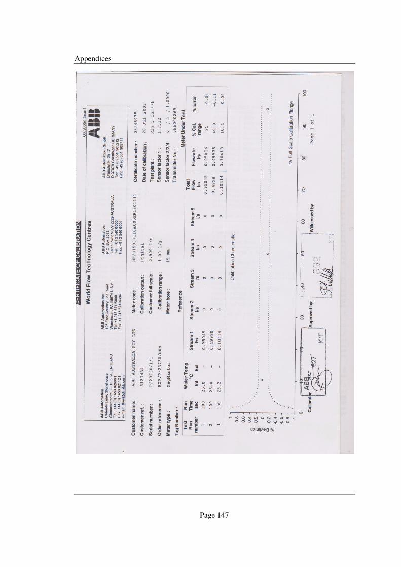
Appendices
Page 147

Appendices
Page 148
Appendix E Level Run to Low and High Header tanks for pressure calibration

Appendices
Page 149
Survey
One
Backsight Foresight Int Rise Fall
RL
(AHD) Comment
1.444 693.809 DW - On door sill 1.665 1.467 0.023 693.786 P1 1.605 1.661 1.652 (Cross at flange) 0.004 693.79 Cross on floor
1.499 1.608 0.003 693.787 P1 1.476 0.023 NA DW - On door sill
Ʃ 6.213 6.212 0.027 0.026
Survey
Two
Backsight Foresight Int Rise Fall
RL
(AHD) Comment
3.328 697.654 Level floor 2-stairwall-arrow 0.786 0.802 2.526 700.18 Lower Header Tank-long edge
3.313 2.527 697.653 Level floor 2-stairwall-arrow Ʃ 4.114 4.115 2.526 2.527 NA
Survey
Three
Backsight Foresight Int Rise Fall
RL
(AHD) Comment
1.534 704.934 Point 'Duff' Level 4 Z block 1.955 0.679 0.855 705.789 P2 1.647 0.128 1.827 707.616 P3 1.874 0.662 0.985 708.601 P4 0.536 0.504 1.37 709.971 High Header Tank-long edge
0.323 1.906 1.37 708.601 P4 0.157 1.308 0.985 707.616 P3 0.584 1.983 1.826 705.79 P2
1.439 0.855 704.935 Point 'Duff' Level 4 Z block Ʃ 8.61 8.609 5.037 5.036 NA
Appendices
Page 150
Appendix F Certificate of Calibration (Digital Multimeter used for Pressure Transducer Calibration)
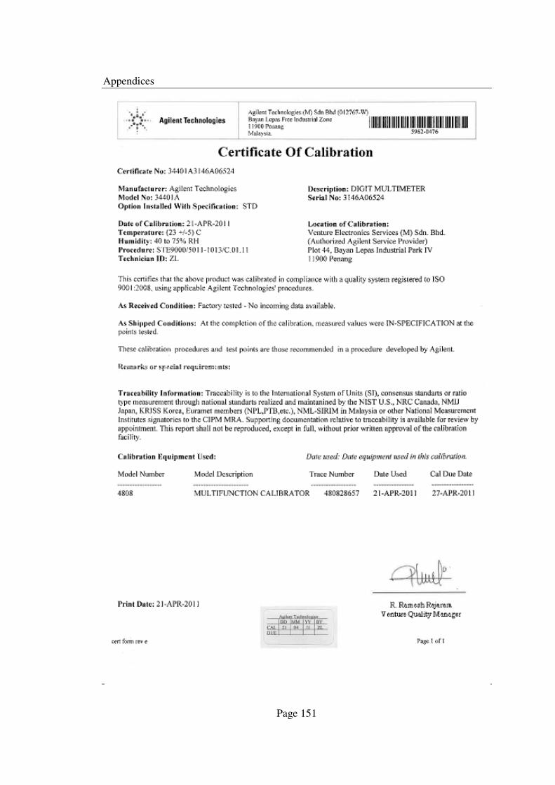
Appendices
Page 151
Appendices
Page 152
Appendix G Labview output for Stage Two-Automatic data acquisition tests for discharges of 0.3 and 0.5 L/s
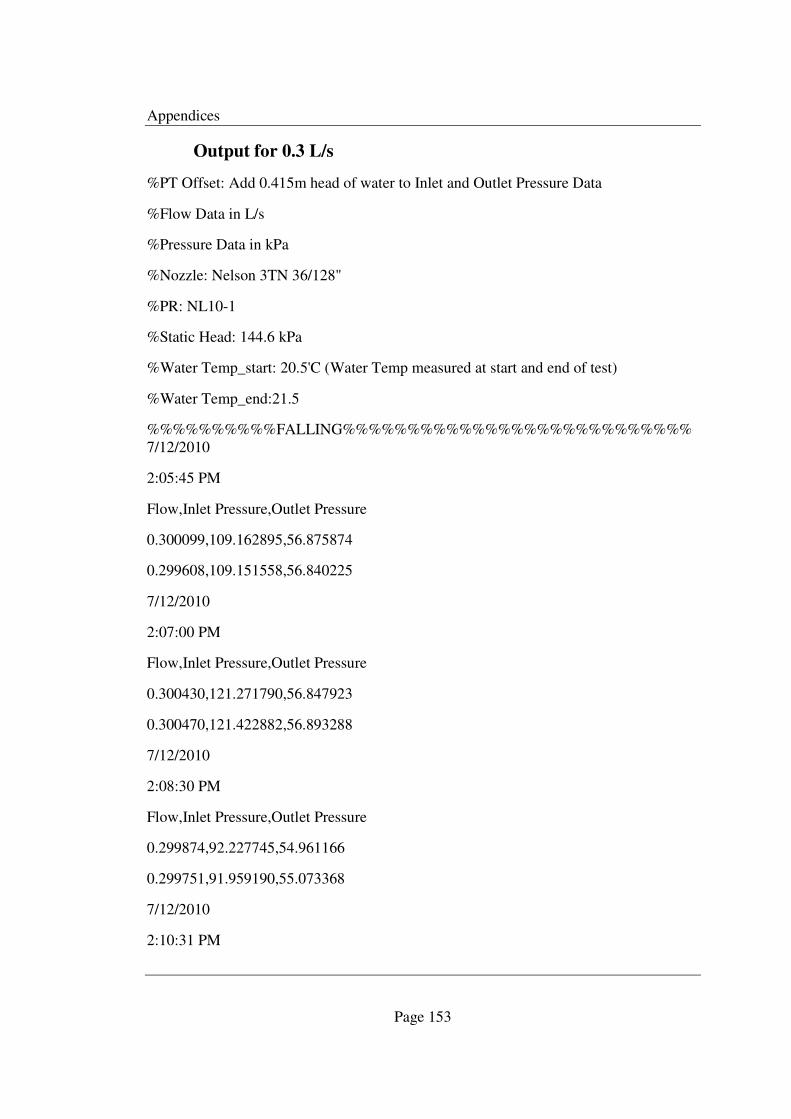
Appendices
Page 153
Output for 0.3 L/s
%PT Offset: Add 0.415m head of water to Inlet and Outlet Pressure Data
%Flow Data in L/s
%Pressure Data in kPa
%Nozzle: Nelson 3TN 36/128"
%PR: NL10-1
%Static Head: 144.6 kPa
%Water Temp_start: 20.5'C (Water Temp measured at start and end of test)
%Water Temp_end:21.5
%%%%%%%%%%FALLING%%%%%%%%%%%%%%%%%%%%%%%%%%%7/12/2010
2:05:45 PM
Flow,Inlet Pressure,Outlet Pressure
0.300099,109.162895,56.875874
0.299608,109.151558,56.840225
7/12/2010
2:07:00 PM
Flow,Inlet Pressure,Outlet Pressure
0.300430,121.271790,56.847923
0.300470,121.422882,56.893288
7/12/2010
2:08:30 PM
Flow,Inlet Pressure,Outlet Pressure
0.299874,92.227745,54.961166
0.299751,91.959190,55.073368
7/12/2010
2:10:31 PM
Appendices
Page 154
Flow,Inlet Pressure,Outlet Pressure
0.299893,63.464939,52.609406
7/12/2010
2:10:36 PM
Flow,Inlet Pressure,Outlet Pressure
0.299989,63.368134,52.642216
0.299591,63.508282,52.594418
7/12/2010
2:12:05 PM
Flow,Inlet Pressure,Outlet Pressure
0.300441,38.028992,32.010265
0.300481,38.063015,32.079124
7/12/2010
2:16:09 PM
Flow,Inlet Pressure,Outlet Pressure
0.300328,112.204498,56.395069
7/12/2010
2:17:36 PM
Flow,Inlet Pressure,Outlet Pressure
0.299841,103.765060,57.059364
0.299845,103.805969,57.257839
7/12/2010
2:17:43 PM
Flow,Inlet Pressure,Outlet Pressure
0.300317,103.867950,57.237183
0.299644,103.980148,57.144020
7/12/2010

Appendices
Page 155
2:18:59 PM
Flow,Inlet Pressure,Outlet Pressure
0.299265,83.174263,57.131058
0.299140,83.151985,57.168728
7/12/2010
2:20:17 PM
Flow,Inlet Pressure,Outlet Pressure
0.299813,78.036903,55.982315
0.300067,78.135338,56.003784
7/12/2010
2:20:26 PM
Flow,Inlet Pressure,Outlet Pressure
0.299417,78.234573,56.043884
7/12/2010
2:21:37 PM
Flow,Inlet Pressure,Outlet Pressure
0.300874,71.221802,54.095558
7/12/2010
2:21:43 PM
Flow,Inlet Pressure,Outlet Pressure
0.299757,71.156181,54.056271
0.300603,71.359924,54.016171
7/12/2010
2:23:19 PM
Flow,Inlet Pressure,Outlet Pressure
0.299973,121.532249,58.519188
0.300626,121.524956,58.587238

Appendices
Page 156
%%%%%%%%%%%%%%RISING%%%%%%%%%%%%%%%%%%%%
7/12/2010
3:09:48 PM
Flow,Inlet Pressure,Outlet Pressure
0.300411,121.422073,65.102180
0.300422,121.510780,64.972160
7/12/2010
3:10:20 PM
Flow,Inlet Pressure,Outlet Pressure
0.299787,118.362640,64.887505
7/12/2010
3:11:33 PM
Flow,Inlet Pressure,Outlet Pressure
0.300283,111.498886,64.824318
7/12/2010
3:12:41 PM
Flow,Inlet Pressure,Outlet Pressure
0.300157,98.707481,64.631508
7/12/2010
3:13:24 PM
Flow,Inlet Pressure,Outlet Pressure
0.299750,85.762589,63.457245
7/12/2010
3:14:14 PM
Flow,Inlet Pressure,Outlet Pressure
0.299462,71.475769,61.352566
7/12/2010
Appendices
Page 157
3:14:16 PM
Flow,Inlet Pressure,Outlet Pressure
0.299411,71.258659,61.380516
7/12/2010
3:15:20 PM
Flow,Inlet Pressure,Outlet Pressure
0.300605,61.266693,54.992355
7/12/2010
3:16:14 PM
Flow,Inlet Pressure,Outlet Pressure
0.299821,48.035099,42.576557
7/12/2010
3:17:20 PM
Flow,Inlet Pressure,Outlet Pressure
0.300609,44.251869,38.970745

Appendices
Page 158
Output for 0.5 L/s
%PT Offset: Add 0.415m head of water to Inlet and Outlet Pressure Data
%Flow Data in L/s
%Pressure Data in kPa
%Nozzle: Nelson 3TN 48/128"
%PR: NL10-1
%Static Head: 144.6 kPa
%Water Temp_start: 20.0'C (Water Temp measured at start and end of test)
%Water Temp_end: 21.5'C
%%%%%%%%%%%%%FALLING%%%%%%%%%%%%%%%
8/12/2010
11:37:38 AM
Flow,Inlet Pressure,Outlet Pressure
0.499983,57.534496,40.564236
0.499899,57.865021,40.364544
8/12/2010
11:41:03 AM
Flow,Inlet Pressure,Outlet Pressure
0.500038,49.300900,32.653088
8/12/2010
11:44:42 AM
Flow,Inlet Pressure,Outlet Pressure
0.500994,55.296959,37.907475
8/12/2010
11:46:45 AM
Flow,Inlet Pressure,Outlet Pressure
0.500072,51.880707,34.978516
Appendices
Page 159
8/12/2010
11:48:17 AM
Flow,Inlet Pressure,Outlet Pressure
0.500300,55.910622,38.423111
0.500518,56.125301,38.529236
8/12/2010
11:49:22 AM
Flow,Inlet Pressure,Outlet Pressure
0.500588,62.419083,44.623306
0.499876,62.552345,44.551613
8/12/2010
11:50:06 AM
Flow,Inlet Pressure,Outlet Pressure
0.500336,65.820755,47.685535
8/12/2010
11:51:34 AM
Flow,Inlet Pressure,Outlet Pressure
0.499843,69.774124,50.658245
8/12/2010
11:52:26 AM
Flow,Inlet Pressure,Outlet Pressure
0.499486,73.780960,51.884758
8/12/2010
11:53:22 AM
Flow,Inlet Pressure,Outlet Pressure
0.500769,77.517212,52.232704
8/12/2010
Appendices
Page 160
11:55:06 AM
Flow,Inlet Pressure,Outlet Pressure
0.500434,84.762093,54.025486
%%%%%%%%%%%%RISING%%%%%%%%%%%%%%%%%%%%%
8/12/2010
11:57:22 AM
Flow,Inlet Pressure,Outlet Pressure
0.499225,83.898506,60.081497
0.499713,84.424683,60.025192
8/12/2010
11:57:26 AM
Flow,Inlet Pressure,Outlet Pressure
0.500278,84.281693,60.034912
0.499560,83.807373,60.384075
8/12/2010
11:58:21 AM
Flow,Inlet Pressure,Outlet Pressure
0.499544,83.347633,60.346405
0.499318,83.399879,60.163319
8/12/2010
12:00:29 PM
Flow,Inlet Pressure,Outlet Pressure
0.500786,81.791801,59.258823
8/12/2010
12:02:15 PM
Flow,Inlet Pressure,Outlet Pressure
0.499751,80.764168,59.315937
Appendices
Page 161
0.499527,80.559204,59.334568
8/12/2010
12:03:31 PM
Flow,Inlet Pressure,Outlet Pressure
0.499598,77.964401,58.216610
0.499316,77.783340,58.145321
8/12/2010
12:04:31 PM
Flow,Inlet Pressure,Outlet Pressure
0.499690,72.385124,53.311775
8/12/2010
12:05:06 PM
Flow,Inlet Pressure,Outlet Pressure
0.499580,65.296616,46.888382
8/12/2010
12:06:13 PM
Flow,Inlet Pressure,Outlet Pressure
0.501185,56.785141,38.746346
8/12/2010
12:06:34 PM
Flow,Inlet Pressure,Outlet Pressure
0.499838,51.375198,33.819244
0.500199,51.150391,33.975189
8/12/2010
12:07:16 PM
Flow,Inlet Pressure,Outlet Pressure
0.500705,48.338486,30.706795
Appendices
Page 162
8/12/2010
12:07:58 PM
Flow,Inlet Pressure,Outlet Pressure
0.500574,48.434486,31.117928
0.500325,48.284615,30.997219
8/12/2010
12:09:22 PM
Flow,Inlet Pressure,Outlet Pressure
0.500188,47.663258,30.058706

Appendices
Page 163
Appendix H Matlab code for Stage two – Automatic data acquisition data processing

Appendices
Page 164
%David Mohr
%0050086160
%ENG4111/ENG4112 Research Project
%Performance Characterization of Pressure Regulation Devices used
%in Broad-acre Irrigation
%Stage Two Script - Automatic data acquisition
%This script inputs the raw textfile produced from the software and
puts
%the flow (L/s), input pressure (kPa) and output pressure (kPa) into
%matlab. Each group is taken individually and kept separate. The
pressure
%transducer offsets are also added in this script and the pressures
%converted from kPa to metres head.
%Clears the associated variables, matlab command window, and closes all
%figures respectively.
clear
clc
close all
%A datafile from the 'Labview' software is inputted into matlab via
matlabs
%textread function. From the output Labview textfile each time the
software
%outputs a time, date and file structure was stamped to each read. The
%textread function takes these stamps and converts this to a value of 0
in
%matlab. This is going to be a standard format. The values of flow,
input

Appendices
Page 165
%and output pressure from the textfile are taken and grouped.
%Value of gravitational acceleration is calculated and used for matlab
%analysis (units = m/s^-2)
g = 9.789278;
%All textfiles on folder are ordered to be brought into script and
named in
%an appropriate way for further analysis.
textfiles = dir('*.txt');
var = 1;
txtnum = length(textfiles);
while var <=txtnum
a = double(textfiles(var).name);
fid = fopen(textfiles(var).name);
%From the called textfile, the matlab function textscan is used to read
the
%file in an appropriate format. Labview outputs the textfile in a
particular
%format and this matlab script has been written to work with that
%particular format and take out the necessary information.
file = textscan(fid, '%f %f %f', 'commentStyle', '%', 'delimiter',...
'/ : , ','treatasempty', {'AM', 'PM',...
'Flow,Inlet Pressure,Outlet Pressure'});
fclose(fid);

Appendices
Page 166
r = length(a)-4;
s = a(12:r);
t = double('Data_PP_');
u = [t s];
name = char(u);
raw_data = cell2mat(file);
b = length(raw_data);
d = 6;
%This loop takes the data extracted from the textfile, and selects and
%writes to a new variable the appropriate information needed and
discards
%the information or gaps through the extracted data.
i = 1; % raw data counter
j = 0; % resolved data counter (Flow, Pressure In, Pressure Out)
k = 1; % used for storage in cases with 2 lines of data.
while i <=b
if raw_data(i,3) > 2000
i = i + 4;
k = 1;
j = j + 1;
if i > b
break
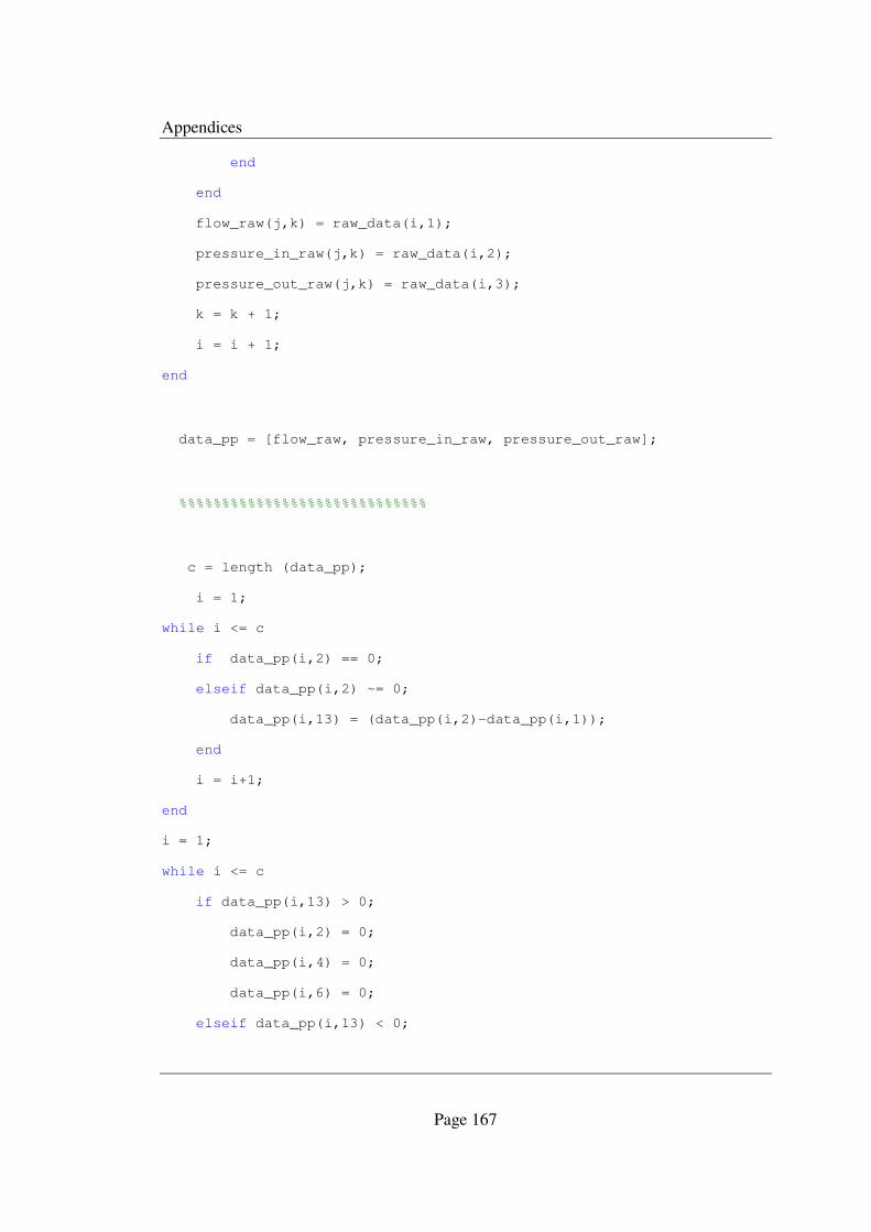
Appendices
Page 167
end
end
flow_raw(j,k) = raw_data(i,1);
pressure_in_raw(j,k) = raw_data(i,2);
pressure_out_raw(j,k) = raw_data(i,3);
k = k + 1;
i = i + 1;
end
data_pp = [flow_raw, pressure_in_raw, pressure_out_raw];
%%%%%%%%%%%%%%%%%%%%%%%%%%%%%
c = length (data_pp);
i = 1;
while i <= c
if data_pp(i,2) == 0;
elseif data_pp(i,2) ~= 0;
data_pp(i,13) = (data_pp(i,2)-data_pp(i,1));
end
i = i+1;
end
i = 1;
while i <= c
if data_pp(i,13) > 0;
data_pp(i,2) = 0;
data_pp(i,4) = 0;
data_pp(i,6) = 0;
elseif data_pp(i,13) < 0;
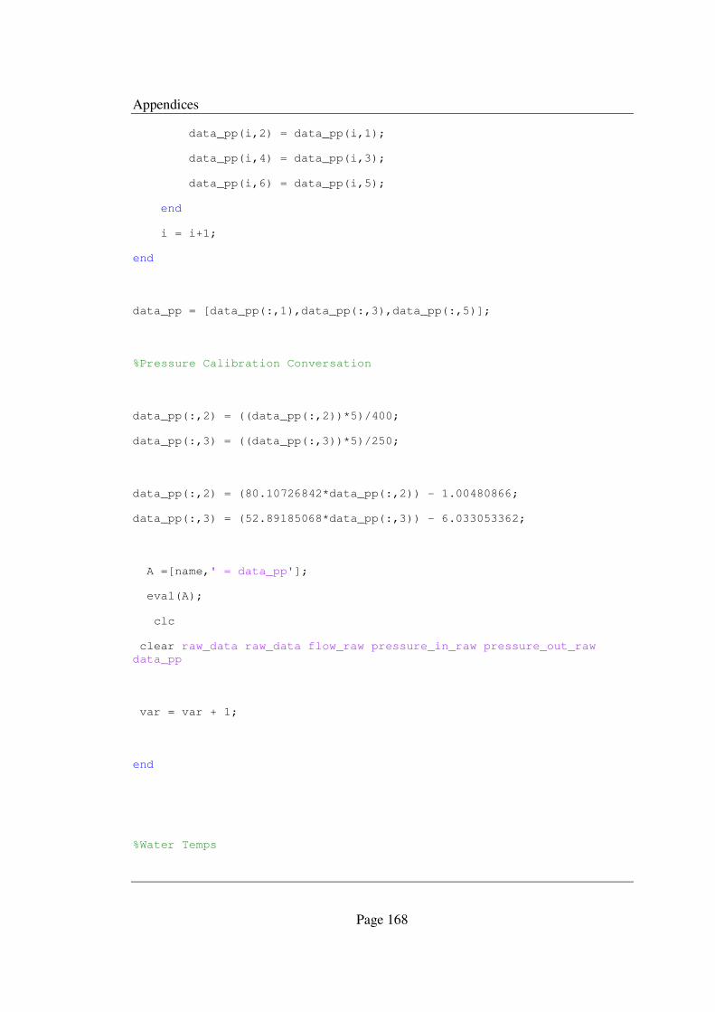
Appendices
Page 168
data_pp(i,2) = data_pp(i,1);
data_pp(i,4) = data_pp(i,3);
data_pp(i,6) = data_pp(i,5);
end
i = i+1;
end
data_pp = [data_pp(:,1),data_pp(:,3),data_pp(:,5)];
%Pressure Calibration Conversation
data_pp(:,2) = ((data_pp(:,2))*5)/400;
data_pp(:,3) = ((data_pp(:,3))*5)/250;
data_pp(:,2) = (80.10726842*data_pp(:,2)) - 1.00480866;
data_pp(:,3) = (52.89185068*data_pp(:,3)) - 6.033053362;
A =[name,' = data_pp'];
eval(A);
clc
clear raw_data raw_data flow_raw pressure_in_raw pressure_out_raw
data_pp
var = var + 1;
end
%Water Temps
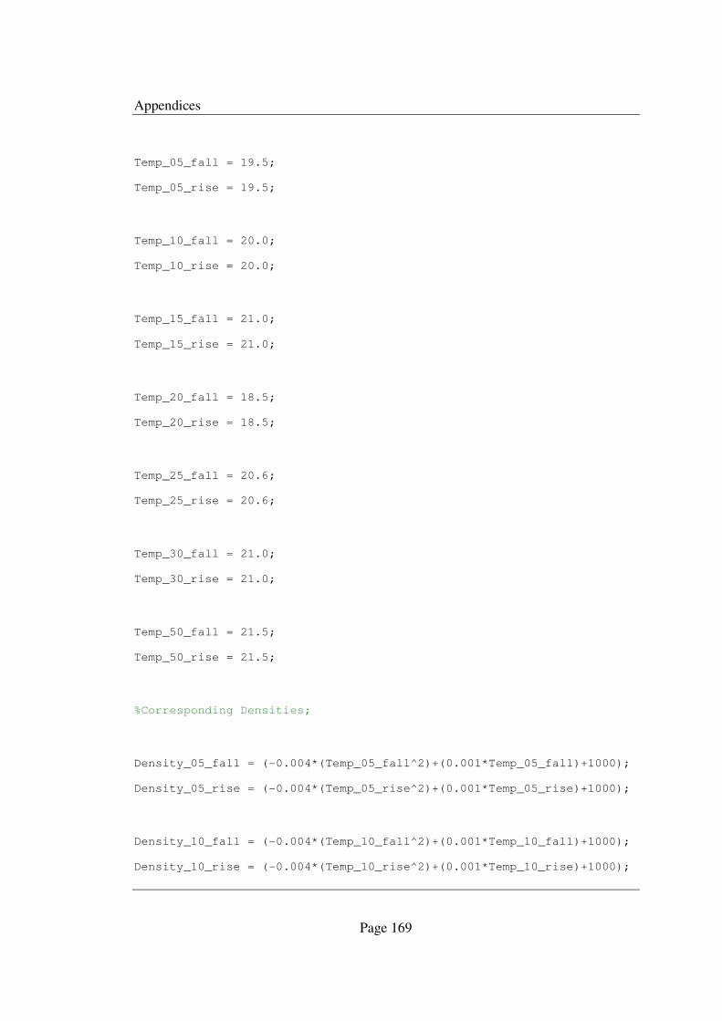
Appendices
Page 169
Temp_05_fall = 19.5;
Temp_05_rise = 19.5;
Temp_10_fall = 20.0;
Temp_10_rise = 20.0;
Temp_15_fall = 21.0;
Temp_15_rise = 21.0;
Temp_20_fall = 18.5;
Temp_20_rise = 18.5;
Temp_25_fall = 20.6;
Temp_25_rise = 20.6;
Temp_30_fall = 21.0;
Temp_30_rise = 21.0;
Temp_50_fall = 21.5;
Temp_50_rise = 21.5;
%Corresponding Densities;
Density_05_fall = (-0.004*(Temp_05_fall^2)+(0.001*Temp_05_fall)+1000);
Density_05_rise = (-0.004*(Temp_05_rise^2)+(0.001*Temp_05_rise)+1000);
Density_10_fall = (-0.004*(Temp_10_fall^2)+(0.001*Temp_10_fall)+1000);
Density_10_rise = (-0.004*(Temp_10_rise^2)+(0.001*Temp_10_rise)+1000);
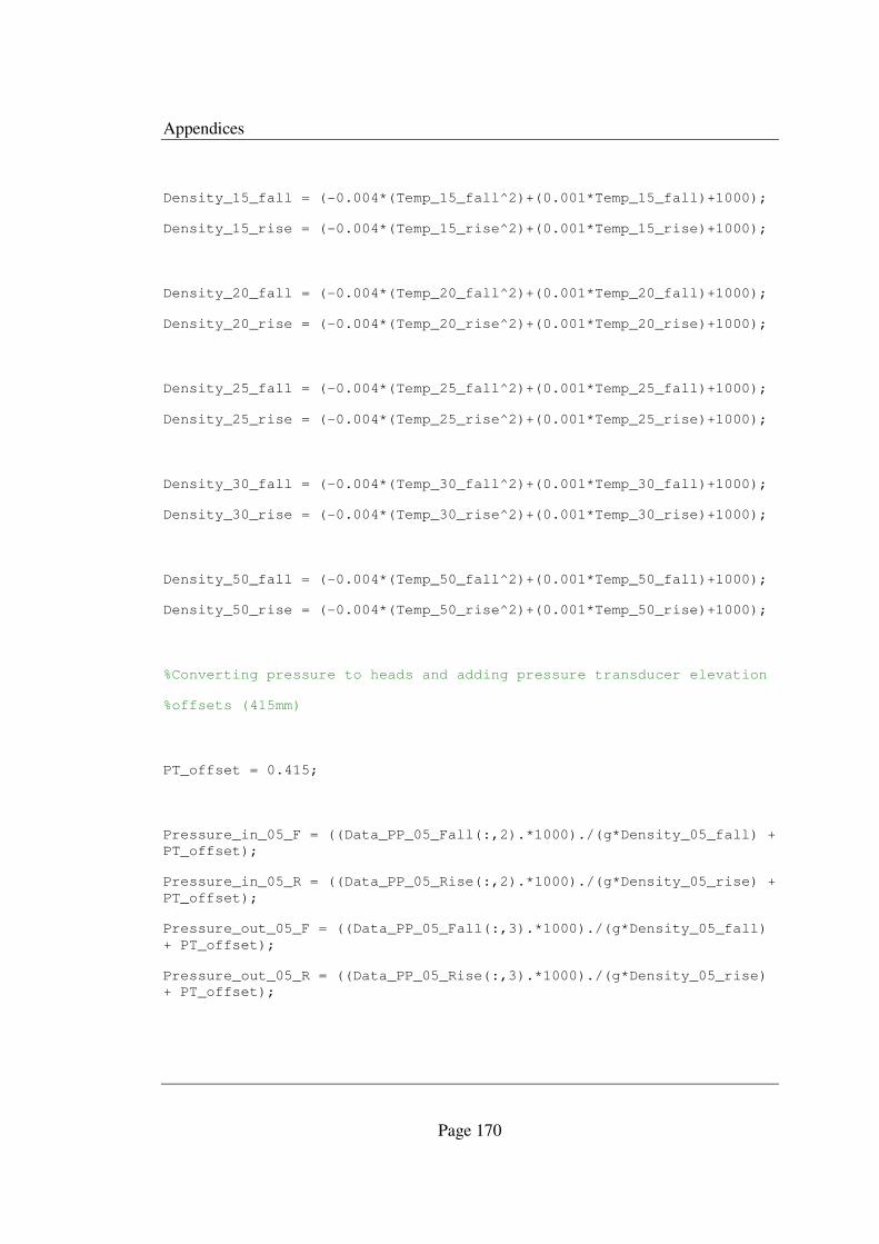
Appendices
Page 170
Density_15_fall = (-0.004*(Temp_15_fall^2)+(0.001*Temp_15_fall)+1000);
Density_15_rise = (-0.004*(Temp_15_rise^2)+(0.001*Temp_15_rise)+1000);
Density_20_fall = (-0.004*(Temp_20_fall^2)+(0.001*Temp_20_fall)+1000);
Density_20_rise = (-0.004*(Temp_20_rise^2)+(0.001*Temp_20_rise)+1000);
Density_25_fall = (-0.004*(Temp_25_fall^2)+(0.001*Temp_25_fall)+1000);
Density_25_rise = (-0.004*(Temp_25_rise^2)+(0.001*Temp_25_rise)+1000);
Density_30_fall = (-0.004*(Temp_30_fall^2)+(0.001*Temp_30_fall)+1000);
Density_30_rise = (-0.004*(Temp_30_rise^2)+(0.001*Temp_30_rise)+1000);
Density_50_fall = (-0.004*(Temp_50_fall^2)+(0.001*Temp_50_fall)+1000);
Density_50_rise = (-0.004*(Temp_50_rise^2)+(0.001*Temp_50_rise)+1000);
%Converting pressure to heads and adding pressure transducer elevation
%offsets (415mm)
PT_offset = 0.415;
Pressure_in_05_F = ((Data_PP_05_Fall(:,2).*1000)./(g*Density_05_fall) +
PT_offset);
Pressure_in_05_R = ((Data_PP_05_Rise(:,2).*1000)./(g*Density_05_rise) +
PT_offset);
Pressure_out_05_F = ((Data_PP_05_Fall(:,3).*1000)./(g*Density_05_fall)
+ PT_offset);
Pressure_out_05_R = ((Data_PP_05_Rise(:,3).*1000)./(g*Density_05_rise)
+ PT_offset);
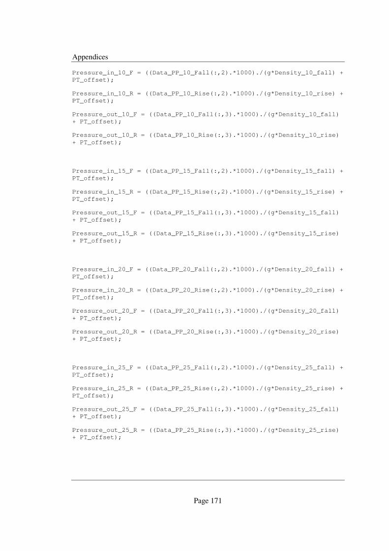
Appendices
Page 171
Pressure_in_10_F = ((Data_PP_10_Fall(:,2).*1000)./(g*Density_10_fall) +
PT_offset);
Pressure_in_10_R = ((Data_PP_10_Rise(:,2).*1000)./(g*Density_10_rise) +
PT_offset);
Pressure_out_10_F = ((Data_PP_10_Fall(:,3).*1000)./(g*Density_10_fall)
+ PT_offset);
Pressure_out_10_R = ((Data_PP_10_Rise(:,3).*1000)./(g*Density_10_rise)
+ PT_offset);
Pressure_in_15_F = ((Data_PP_15_Fall(:,2).*1000)./(g*Density_15_fall) +
PT_offset);
Pressure_in_15_R = ((Data_PP_15_Rise(:,2).*1000)./(g*Density_15_rise) +
PT_offset);
Pressure_out_15_F = ((Data_PP_15_Fall(:,3).*1000)./(g*Density_15_fall)
+ PT_offset);
Pressure_out_15_R = ((Data_PP_15_Rise(:,3).*1000)./(g*Density_15_rise)
+ PT_offset);
Pressure_in_20_F = ((Data_PP_20_Fall(:,2).*1000)./(g*Density_20_fall) +
PT_offset);
Pressure_in_20_R = ((Data_PP_20_Rise(:,2).*1000)./(g*Density_20_rise) +
PT_offset);
Pressure_out_20_F = ((Data_PP_20_Fall(:,3).*1000)./(g*Density_20_fall)
+ PT_offset);
Pressure_out_20_R = ((Data_PP_20_Rise(:,3).*1000)./(g*Density_20_rise)
+ PT_offset);
Pressure_in_25_F = ((Data_PP_25_Fall(:,2).*1000)./(g*Density_25_fall) +
PT_offset);
Pressure_in_25_R = ((Data_PP_25_Rise(:,2).*1000)./(g*Density_25_rise) +
PT_offset);
Pressure_out_25_F = ((Data_PP_25_Fall(:,3).*1000)./(g*Density_25_fall)
+ PT_offset);
Pressure_out_25_R = ((Data_PP_25_Rise(:,3).*1000)./(g*Density_25_rise)
+ PT_offset);
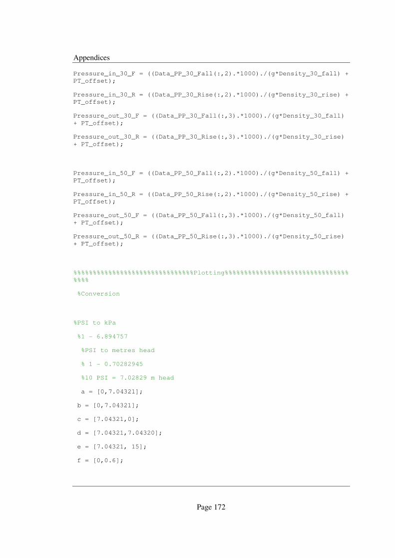
Appendices
Page 172
Pressure_in_30_F = ((Data_PP_30_Fall(:,2).*1000)./(g*Density_30_fall) +
PT_offset);
Pressure_in_30_R = ((Data_PP_30_Rise(:,2).*1000)./(g*Density_30_rise) +
PT_offset);
Pressure_out_30_F = ((Data_PP_30_Fall(:,3).*1000)./(g*Density_30_fall)
+ PT_offset);
Pressure_out_30_R = ((Data_PP_30_Rise(:,3).*1000)./(g*Density_30_rise)
+ PT_offset);
Pressure_in_50_F = ((Data_PP_50_Fall(:,2).*1000)./(g*Density_50_fall) +
PT_offset);
Pressure_in_50_R = ((Data_PP_50_Rise(:,2).*1000)./(g*Density_50_rise) +
PT_offset);
Pressure_out_50_F = ((Data_PP_50_Fall(:,3).*1000)./(g*Density_50_fall)
+ PT_offset);
Pressure_out_50_R = ((Data_PP_50_Rise(:,3).*1000)./(g*Density_50_rise)
+ PT_offset);
%%%%%%%%%%%%%%%%%%%%%%%%%%%%%%%Plotting%%%%%%%%%%%%%%%%%%%%%%%%%%%%%%%%
%%%%
%Conversion
%PSI to kPa
%1 - 6.894757
%PSI to metres head
% 1 - 0.70282945
%10 PSI = 7.02829 m head
a = [0,7.04321];
b = [0,7.04321];
c = [7.04321,0];
d = [7.04321,7.04320];
e = [7.04321, 15];
f = [0,0.6];
Appendices
Page 173
plot( Pressure_in_05_F(:,1), Pressure_out_05_F(:,1), 'red +',
Pressure_in_05_R(:,1), Pressure_out_05_R(:,1), 'bl +', a, b, 'k --',
c, d, 'k --', d, c, 'k --', e, d, 'k --');
xlabel('Hpi Input Pressure Head (m)');
ylabel('Hpo Output Pressure Head (m)');
title('Flow - 0.05 L/s')
legend('0.05 L/s-Fall', '0.05 L/s-Rise')
grid on
figure
plot( Pressure_in_10_F(:,1), Pressure_out_10_F(:,1), 'red +',
Pressure_in_10_R(:,1), Pressure_out_10_R(:,1), 'bl +', a, b, 'k --',
c, d, 'k --', d, c, 'k --', e, d, 'k --');
xlabel('Hpi Input Pressure Head (m)');
ylabel('Hpo Output Pressure Head (m)');
title('Flow - 0.10 L/s')
legend('0.10 L/s-Fall', '0.10 L/s-Rise')
grid on
figure
plot( Pressure_in_15_F(:,1), Pressure_out_15_F(:,1), 'red +',
Pressure_in_15_R(:,1), Pressure_out_15_R(:,1), 'bl +', a, b, 'k --',
c, d, 'k --', d, c, 'k --', e, d, 'k --');
xlabel('Hpi Input Pressure Head (m)');
ylabel('Hpo Output Pressure Head (m)');
title('Flow - 0.15 L/s')
legend('0.15 L/s-Fall', '0.15 L/s-Rise')
grid on
figure
plot( Pressure_in_20_F(:,1), Pressure_out_20_F(:,1), 'red +',
Pressure_in_20_R(:,1), Pressure_out_20_R(:,1), 'bl +', a, b, 'k --',
c, d, 'k --', d, c, 'k --', e, d, 'k --');
xlabel('Hpi Input Pressure Head (m)');
ylabel('Hpo Output Pressure Head (m)');
title('Flow - 0.20 L/s')
Appendices
Page 174
legend('0.20 L/s-Fall', '0.20 L/s-Rise')
grid on
figure
plot( Pressure_in_25_F(:,1), Pressure_out_25_F(:,1), 'red +',
Pressure_in_25_R(:,1), Pressure_out_25_R(:,1), 'bl +', a, b, 'k --',
c, d, 'k --', d, c, 'k --', e, d, 'k --');
xlabel('Hpi Input Pressure Head (m)');
ylabel('Hpo Output Pressure Head (m)');
title('Flow - 0.25 L/s')
legend('0.25 L/s-Fall', '0.25 L/s-Rise')
grid on
figure
plot( Pressure_in_30_F(:,1), Pressure_out_30_F(:,1), 'red +',
Pressure_in_30_R(:,1), Pressure_out_30_R(:,1), 'bl +', a, b, 'k --',
c, d, 'k --', d, c, 'k --', e, d, 'k --');
xlabel('Hpi Input Pressure Head (m)');
ylabel('Hpo Output Pressure Head (m)');
title('Flow - 0.30 L/s')
legend('0.30 L/s-Fall', '0.30 L/s-Rise')
grid on
figure
plot( Pressure_in_50_F(:,1), Pressure_out_50_F(:,1), 'red +',
Pressure_in_50_R(:,1), Pressure_out_50_R(:,1), 'bl +', a, b, 'k --',
c, d, 'k --', d, c, 'k --', e, d, 'k --');
xlabel('Hpi Input Pressure Head (m)');
ylabel('Hpo Output Pressure Head (m)');
title('Flow - 0.50 L/s')
legend('0.50 L/s-Fall', '0.50 L/s-Rise')
grid on
% Rising Falling 2D Plot
figure
plot(Pressure_in_05_F(:,1), Pressure_out_05_F(:,1), 'red +',...
Pressure_in_05_R(:,1), Pressure_out_05_R(:,1), 'bl +',...
Appendices
Page 175
Pressure_in_10_F(:,1), Pressure_out_10_F(:,1), 'red o',...
Pressure_in_10_R(:,1), Pressure_out_10_R(:,1), 'bl o',...
Pressure_in_15_F(:,1), Pressure_out_15_F(:,1), 'red *',...
Pressure_in_15_R(:,1), Pressure_out_15_R(:,1), 'bl *',...
Pressure_in_20_F(:,1), Pressure_out_20_F(:,1), 'red d',...
Pressure_in_20_R(:,1), Pressure_out_20_R(:,1), 'bl d', ...
Pressure_in_25_F(:,1), Pressure_out_25_F(:,1), 'red s',...
Pressure_in_25_R(:,1), Pressure_out_25_R(:,1), 'bl s',...
Pressure_in_30_F(:,1), Pressure_out_30_F(:,1), 'red >',...
Pressure_in_30_R(:,1), Pressure_out_30_R(:,1), 'bl >',...
Pressure_in_50_F(:,1), Pressure_out_50_F(:,1), 'red p',...
Pressure_in_50_R(:,1), Pressure_out_50_R(:,1), 'bl p',...
a, b, 'k --', c, d, 'k --', d, c, 'k --', e, d, 'k --');
xlabel('Hpi Input Pressure Head (m)');
ylabel('Hpo Output Pressure Head (m)');
%title('All Discharges');
grid on
legend('0.05 L/s-Fall', '0.05 L/s-Rise', '0.10 L/s-Fall',...
'0.10 L/s-Rise','0.15 L/s-Fall', '0.15 L/s-Rise','0.20 L/s-
Fall',...
'0.20 L/s-Rise','0.25 L/s-Fall', '0.25 L/s-Rise','0.30 L/s-
Fall',...
'0.30 L/s-Rise', '0.50 L/s-Fall', '0.50 L/s-Rise',...
'Location', 'SouthEast');
%%%%%%%%%%%%%%Three Dimensional Plot%%%%%%%%%%%%%%%%%%%
figure
plot3 (Pressure_in_05_F(:,1),Data_PP_05_Fall(:,1) ,
Pressure_out_05_F(:,1), 'red +')

Appendices
Page 176
hold on
plot3 (Pressure_in_05_R(:,1),Data_PP_05_Rise(:,1) ,
Pressure_out_05_R(:,1), 'bl +')
hold on
plot3 (Pressure_in_10_F(:,1),Data_PP_10_Fall(:,1) ,
Pressure_out_10_F(:,1), 'red x')
hold on
plot3 (Pressure_in_10_R(:,1),Data_PP_10_Rise(:,1) ,
Pressure_out_10_R(:,1), 'bl x')
hold on
plot3 (Pressure_in_15_F(:,1),Data_PP_15_Fall(:,1) ,
Pressure_out_15_F(:,1), 'red o')
hold on
plot3 (Pressure_in_15_R(:,1),Data_PP_15_Rise(:,1) ,
Pressure_out_15_R(:,1), 'bl o')
hold on
plot3 (Pressure_in_20_F(:,1),Data_PP_20_Fall(:,1) ,
Pressure_out_20_F(:,1), 'red s')
hold on
plot3 (Pressure_in_20_R(:,1),Data_PP_20_Rise(:,1) ,
Pressure_out_20_R(:,1), 'bl s')
hold on
plot3 (Pressure_in_25_F(:,1),Data_PP_25_Fall(:,1) ,
Pressure_out_25_F(:,1), 'red *')
hold on
plot3 (Pressure_in_25_R(:,1),Data_PP_25_Rise(:,1) ,
Pressure_out_25_R(:,1), 'bl *')
hold on
plot3 (Pressure_in_30_F(:,1),Data_PP_30_Fall(:,1) ,
Pressure_out_30_F(:,1), 'red d')
hold on
plot3 (Pressure_in_30_R(:,1),Data_PP_30_Rise(:,1) ,
Pressure_out_30_R(:,1), 'bl d')
hold on
Appendices
Page 177
plot3 (Pressure_in_50_F(:,1),Data_PP_50_Fall(:,1) ,
Pressure_out_50_F(:,1), 'red o')
hold on
plot3 (Pressure_in_50_R(:,1),Data_PP_50_Rise(:,1) ,
Pressure_out_50_R(:,1), 'bl o')
grid on
xlabel('Hpi Input Pressure Head (m)');
zlabel('Hpo Output Pressure Head (m)');
ylabel('Flow Rate (L/s)');
%title('All Discharges 3D plot');
grid on
legend('0.05 L/s-Fall', '0.05 L/s-Rise', '0.10 L/s-Fall',...
'0.10 L/s-Rise','0.15 L/s-Fall', '0.15 L/s-Rise','0.20 L/s-
Fall',...
'0.20 L/s-Rise','0.25 L/s-Fall', '0.25 L/s-Rise','0.30 L/s-
Fall',...
'0.30 L/s-Rise', '0.50 L/s-Fall', '0.50 L/s-Rise',...
'Location', 'SouthEast');
%legend('Falling (0.3 L/s)','Rising (0.3 L/s)','Falling (0.5 L/s)',
'Rising
%(0.5 L/s)');
%%%%%%%%%%%%%%%%%%%%%%%%%%%%%%%%%%%%%%%%%%%%%%%%%%%%%%%
figure
plot (Data_PP_05_Fall(:,1) , Pressure_out_05_F(:,1), 'red +')
hold on
plot (Data_PP_05_Rise(:,1) , Pressure_out_05_R(:,1), 'bl +')
hold on
plot (Data_PP_10_Fall(:,1) , Pressure_out_10_F(:,1), 'red x')
hold on
plot (Data_PP_10_Rise(:,1) , Pressure_out_10_R(:,1), 'bl x')
hold on
plot (Data_PP_15_Fall(:,1) , Pressure_out_15_F(:,1), 'red o')
Appendices
Page 178
hold on
plot (Data_PP_15_Rise(:,1) , Pressure_out_15_R(:,1), 'bl o')
hold on
plot (Data_PP_20_Fall(:,1) , Pressure_out_20_F(:,1), 'red s')
hold on
plot (Data_PP_20_Rise(:,1) , Pressure_out_20_R(:,1), 'bl s')
hold on
plot (Data_PP_25_Fall(:,1) , Pressure_out_25_F(:,1), 'red *')
hold on
plot (Data_PP_25_Rise(:,1) , Pressure_out_25_R(:,1), 'bl *')
hold on
plot (Data_PP_30_Fall(:,1) , Pressure_out_30_F(:,1), 'red d')
hold on
plot (Data_PP_30_Rise(:,1) , Pressure_out_30_R(:,1), 'bl d')
hold on
plot (Data_PP_50_Fall(:,1) , Pressure_out_50_F(:,1), 'red o')
hold on
plot (Data_PP_50_Rise(:,1) , Pressure_out_50_R(:,1), 'bl o')
%plot (c, d, 'k --', f, d, 'k --');
plot (f, d, 'k --', 'LineWidth',2);
grid on
ylabel('Hpo Output Pressure Head (m)','FontSize',14);
xlabel('Flow Rate (L/s)','FontSize',14);
%title('All Discharges 3D plot');
grid on
legend('0.05 L/s-Fall', '0.05 L/s-Rise', '0.10 L/s-Fall',...
'0.10 L/s-Rise','0.15 L/s-Fall', '0.15 L/s-Rise','0.20 L/s-
Fall',...
'0.20 L/s-Rise','0.25 L/s-Fall', '0.25 L/s-Rise','0.30 L/s-
Fall',...

Appendices
Page 179
'0.30 L/s-Rise', '0.50 L/s-Fall', '0.50 L/s-Rise',...
'Location', 'SouthEast');
%EOF

Appendices
Page 180
Appendix I Southern Cross Pump Curve HX-C Pump’s performance curve
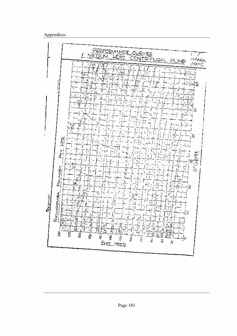
Appendices
Page 181

Appendices
Page 182
Appendix J Labview output for Stage Three-Automatic data acquisition tests with higher heads for discharges of 0.3 and 0.6 L/s
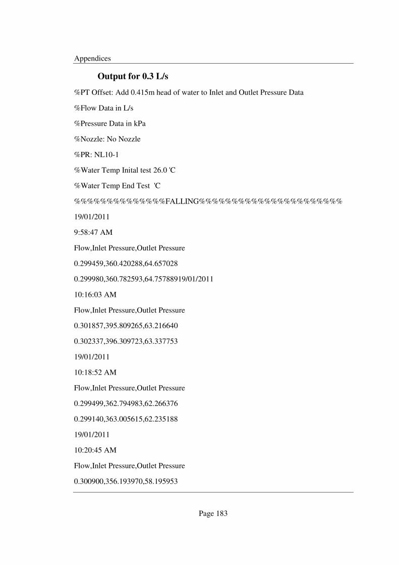
Appendices
Page 183
Output for 0.3 L/s
%PT Offset: Add 0.415m head of water to Inlet and Outlet Pressure Data
%Flow Data in L/s
%Pressure Data in kPa
%Nozzle: No Nozzle
%PR: NL10-1
%Water Temp Inital test 26.0 'C
%Water Temp End Test 'C
%%%%%%%%%%%%%%FALLING%%%%%%%%%%%%%%%%%%%%%%
19/01/2011
9:58:47 AM
Flow,Inlet Pressure,Outlet Pressure
0.299459,360.420288,64.657028
0.299980,360.782593,64.75788919/01/2011
10:16:03 AM
Flow,Inlet Pressure,Outlet Pressure
0.301857,395.809265,63.216640
0.302337,396.309723,63.337753
19/01/2011
10:18:52 AM
Flow,Inlet Pressure,Outlet Pressure
0.299499,362.794983,62.266376
0.299140,363.005615,62.235188
19/01/2011
10:20:45 AM
Flow,Inlet Pressure,Outlet Pressure
0.300900,356.193970,58.195953

Appendices
Page 184
0.300948,355.074036,57.629280
19/01/2011
10:21:25 AM
Flow,Inlet Pressure,Outlet Pressure
0.299716,350.880096,57.412979
0.299953,351.520416,57.622799
19/01/2011
10:22:03 AM
Flow,Inlet Pressure,Outlet Pressure
0.300521,333.616364,56.607723
19/01/2011
10:22:45 AM
Flow,Inlet Pressure,Outlet Pressure
0.300508,321.338593,55.927227
19/01/2011
10:23:50 AM
Flow,Inlet Pressure,Outlet Pressure
0.300109,311.003845,57.688416
19/01/2011
10:24:27 AM
Flow,Inlet Pressure,Outlet Pressure
0.299169,297.082520,56.001759
0.299014,296.503113,55.648548
19/01/2011
10:25:14 AM
Flow,Inlet Pressure,Outlet Pressure
0.299993,278.201233,57.435257
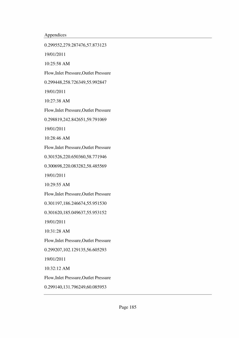
Appendices
Page 185
0.299552,279.287476,57.873123
19/01/2011
10:25:58 AM
Flow,Inlet Pressure,Outlet Pressure
0.299448,258.726349,55.992847
19/01/2011
10:27:38 AM
Flow,Inlet Pressure,Outlet Pressure
0.298819,242.842651,59.791069
19/01/2011
10:28:46 AM
Flow,Inlet Pressure,Outlet Pressure
0.301526,220.650360,58.771946
0.300698,220.083282,58.485569
19/01/2011
10:29:55 AM
Flow,Inlet Pressure,Outlet Pressure
0.301197,186.246674,55.951530
0.301620,185.049637,55.953152
19/01/2011
10:31:28 AM
Flow,Inlet Pressure,Outlet Pressure
0.299207,102.129135,56.605293
19/01/2011
10:32:12 AM
Flow,Inlet Pressure,Outlet Pressure
0.299140,131.796249,60.085953
Appendices
Page 186
19/01/2011
10:33:06 AM
Flow,Inlet Pressure,Outlet Pressure
0.299526,112.342422,55.606827
0.299774,113.083839,56.254108
19/01/2011
10:34:37 AM
Flow,Inlet Pressure,Outlet Pressure
0.298830,152.301956,61.707397
0.298529,152.704437,61.993771
19/01/2011
10:35:26 AM
Flow,Inlet Pressure,Outlet Pressure
0.299311,179.973083,64.462601
19/01/2011
10:36:08 AM
Flow,Inlet Pressure,Outlet Pressure
0.300631,190.758728,56.233452
19/01/2011
10:37:22 AM
Flow,Inlet Pressure,Outlet Pressure
0.299495,126.505203,56.817947
0.299521,126.130608,57.179665
19/01/2011
10:37:53 AM
Flow,Inlet Pressure,Outlet Pressure
0.300244,61.474384,53.942448

Appendices
Page 187
19/01/2011
10:38:22 AM
Flow,Inlet Pressure,Outlet Pressure
0.298669,121.909576,58.906017
19/01/2011
10:39:19 AM
Flow,Inlet Pressure,Outlet Pressure
0.300153,90.471260,58.569012
19/01/2011
10:39:49 AM
Flow,Inlet Pressure,Outlet Pressure
0.298469,57.222267,51.161732
0.298859,57.243008,51.237885
%%%%%%%%%%%RISING%%%%%%%%%%%%
19/01/2011
9:29:57 AM
Flow,Inlet Pressure,Outlet Pressure
0.302131,79.617676,64.120728
0.302364,80.188644,64.603966
19/01/2011
9:30:54 AM
Flow,Inlet Pressure,Outlet Pressure
0.300714,56.623432,50.300175
0.300024,56.701851,50.181496
19/01/2011
9:33:32 AM
Flow,Inlet Pressure,Outlet Pressure
Appendices
Page 188
0.300220,71.999367,62.025772
0.300685,72.125099,61.922482
19/01/2011
9:34:24 AM
Flow,Inlet Pressure,Outlet Pressure
0.299535,93.576912,65.567192
0.300186,93.427200,65.063705
19/01/2011
9:35:08 AM
Flow,Inlet Pressure,Outlet Pressure
0.298354,122.407959,66.527580
19/01/2011
9:36:17 AM
Flow,Inlet Pressure,Outlet Pressure
0.300007,137.412628,67.595718
0.299397,138.260330,67.878853
19/01/2011
9:37:37 AM
Flow,Inlet Pressure,Outlet Pressure
0.299830,145.046539,67.269241
0.299229,145.217636,66.990562
19/01/2011
9:39:28 AM
Flow,Inlet Pressure,Outlet Pressure
0.301992,150.664871,67.505394
0.302348,150.158707,67.191071
19/01/2011

Appendices
Page 189
9:41:11 AM
Flow,Inlet Pressure,Outlet Pressure
0.301502,160.460846,66.434013
0.301276,160.828964,66.314926
19/01/2011
9:42:44 AM
Flow,Inlet Pressure,Outlet Pressure
0.298407,176.658066,68.146599
19/01/2011
9:43:54 AM
Flow,Inlet Pressure,Outlet Pressure
0.301376,175.387146,62.551132
19/01/2011
9:44:19 AM
Flow,Inlet Pressure,Outlet Pressure
0.301300,185.128052,66.207588
0.300339,185.107315,65.924454
19/01/2011
9:46:45 AM
Flow,Inlet Pressure,Outlet Pressure
0.299900,227.194885,65.262589
19/01/2011
9:47:22 AM
Flow,Inlet Pressure,Outlet Pressure
0.299892,248.917313,68.724617
19/01/2011
9:48:55 AM

Appendices
Page 190
Flow,Inlet Pressure,Outlet Pressure
0.299987,276.878448,68.046547
19/01/2011
9:50:38 AM
Flow,Inlet Pressure,Outlet Pressure
0.301389,305.087280,68.629829
19/01/2011
9:51:08 AM
Flow,Inlet Pressure,Outlet Pressure
0.298842,333.538605,69.175850
0.298485,334.144592,69.286026
19/01/2011
9:52:40 AM
Flow,Inlet Pressure,Outlet Pressure
0.300778,338.276917,67.850906
0.300279,337.613251,67.639870
19/01/2011
9:53:08 AM
Flow,Inlet Pressure,Outlet Pressure
0.300430,349.855438,69.602783
0.300951,350.250793,69.855942
19/01/2011
9:53:46 AM
Flow,Inlet Pressure,Outlet Pressure
0.300771,369.961823,68.746490
0.300809,369.644897,68.771606

Appendices
Page 191
Output for 0.6 L/s
%PT Offset: Add 0.415m head of water to Inlet and Outlet Pressure Data
%Flow Data in L/s
%Pressure Data in kPa
%Nozzle: No Nozzle
%PR: NL10-1
%Water Temp Inital test 23.0 'C
%Water Temp End Test 25.0 'C
%%%%%%%%%%%%%FALLING%%%%%%%%%%%%%%%%
16/12/2010
8:16:23 AM
Flow,Inlet Pressure,Outlet Pressure
0.600000,319.580261,55.777763
0.600003,318.547821,55.883076
16/12/2010
8:17:44 AM
Flow,Inlet Pressure,Outlet Pressure
0.602484,271.770081,56.374413
0.602943,270.617126,55.926823
16/12/2010
8:19:01 AM
Flow,Inlet Pressure,Outlet Pressure
0.601781,245.468109,58.678783
0.602240,245.757812,58.424404
16/12/2010
8:19:47 AM
Flow,Inlet Pressure,Outlet Pressure

Appendices
Page 192
0.600144,217.824005,56.753139
16/12/2010
8:20:53 AM
Flow,Inlet Pressure,Outlet Pressure
0.600692,192.913666,56.656330
0.601287,192.998566,56.706558
16/12/2010
8:21:56 AM
Flow,Inlet Pressure,Outlet Pressure
0.599285,136.677689,56.273552
16/12/2010
8:22:31 AM
Flow,Inlet Pressure,Outlet Pressure
0.599014,81.209381,51.763645
16/12/2010
8:23:16 AM
Flow,Inlet Pressure,Outlet Pressure
0.598667,68.444595,40.966053
16/12/2010
8:24:27 AM
Flow,Inlet Pressure,Outlet Pressure
0.599267,81.610550,53.263573
16/12/2010
8:28:26 AM
Flow,Inlet Pressure,Outlet Pressure
0.599910,399.979797,56.551422
0.599974,399.914337,56.250465
Appendices
Page 193
16/12/2010
8:31:20 AM
Flow,Inlet Pressure,Outlet Pressure
0.600463,396.638794,54.823448
16/12/2010
8:33:36 AM
Flow,Inlet Pressure,Outlet Pressure
0.600568,389.032593,59.580845
16/12/2010
8:35:41 AM
Flow,Inlet Pressure,Outlet Pressure
0.600619,369.782928,53.767868
16/12/2010
8:36:49 AM
Flow,Inlet Pressure,Outlet Pressure
0.601225,358.014496,54.582844
0.602074,357.942566,54.651299
16/12/2010
8:37:37 AM
Flow,Inlet Pressure,Outlet Pressure
0.602865,342.188263,54.238544
16/12/2010
8:40:05 AM
Flow,Inlet Pressure,Outlet Pressure
0.603392,318.682648,55.251999
16/12/2010
8:41:45 AM
Appendices
Page 194
Flow,Inlet Pressure,Outlet Pressure
0.601904,277.623779,53.717236
16/12/2010
8:43:05 AM
Flow,Inlet Pressure,Outlet Pressure
0.603241,234.732300,54.459705
16/12/2010
8:44:18 AM
Flow,Inlet Pressure,Outlet Pressure
0.600379,202.068054,55.052303
16/12/2010
8:45:16 AM
Flow,Inlet Pressure,Outlet Pressure
0.602595,138.605118,55.856747
16/12/2010
8:45:37 AM
Flow,Inlet Pressure,Outlet Pressure
0.600346,97.270386,53.578709
16/12/2010
8:46:43 AM
Flow,Inlet Pressure,Outlet Pressure
0.609371,114.103943,55.466679
16/12/2010
8:48:01 AM
Flow,Inlet Pressure,Outlet Pressure
0.603035,108.009277,54.926331
16/12/2010
Appendices
Page 195
8:48:35 AM
Flow,Inlet Pressure,Outlet Pressure
0.601090,67.545692,40.377911
16/12/2010
8:51:15 AM
Flow,Inlet Pressure,Outlet Pressure
0.598705,391.251740,59.823071
%%%%%%%%%%%%%%%%%%%%%%RISING%%%%%%%%%%%%%%%%%%%%%%%%%%
16/12/2010
8:57:05 AM
Flow,Inlet Pressure,Outlet Pressure
0.599256,383.763397,61.786381
16/12/2010
8:57:40 AM
Flow,Inlet Pressure,Outlet Pressure
0.599398,375.866791,61.924911
16/12/2010
8:59:28 AM
Flow,Inlet Pressure,Outlet Pressure
0.599017,374.680725,62.527637
16/12/2010
9:00:40 AM
Flow,Inlet Pressure,Outlet Pressure
0.600191,364.478149,61.016369
16/12/2010
9:01:18 AM

Appendices
Page 196
Flow,Inlet Pressure,Outlet Pressure
0.598811,354.396088,63.030315
16/12/2010
9:02:45 AM
Flow,Inlet Pressure,Outlet Pressure
0.599294,337.568542,63.215832
16/12/2010
9:04:41 AM
Flow,Inlet Pressure,Outlet Pressure
0.600029,311.274109,63.027477
16/12/2010
9:05:22 AM
Flow,Inlet Pressure,Outlet Pressure
0.599781,299.593933,62.849659
0.598563,298.543335,62.736244
16/12/2010
9:05:52 AM
Flow,Inlet Pressure,Outlet Pressure
0.599108,280.987457,64.066452
16/12/2010
9:06:46 AM
Flow,Inlet Pressure,Outlet Pressure
0.599174,255.431396,63.392029
16/12/2010
9:08:20 AM
Flow,Inlet Pressure,Outlet Pressure
0.600053,228.974579,64.039719

Appendices
Page 197
16/12/2010
9:09:31 AM
Flow,Inlet Pressure,Outlet Pressure
0.599189,187.829971,64.484879
16/12/2010
9:10:10 AM
Flow,Inlet Pressure,Outlet Pressure
0.601112,103.313194,61.712662
16/12/2010
9:11:13 AM
Flow,Inlet Pressure,Outlet Pressure
0.595778,136.428818,64.167313
16/12/2010
9:11:35 AM
Flow,Inlet Pressure,Outlet Pressure
0.600568,71.136108,43.639423
16/12/2010
9:13:13 AM
Flow,Inlet Pressure,Outlet Pressure
0.600523,101.627510,62.115696
16/12/2010
9:14:12 AM
Flow,Inlet Pressure,Outlet Pressure
0.599048,159.005859,63.413094
16/12/2010
9:15:57 AM
Flow,Inlet Pressure,Outlet Pressure
Appendices
Page 198
0.596781,268.638458,63.596180
16/12/2010
9:17:18 AM
Flow,Inlet Pressure,Outlet Pressure
0.598988,301.804626,63.197601
0.597923,295.660553,59.954716
16/12/2010
9:17:49 AM
Flow,Inlet Pressure,Outlet Pressure
0.597962,329.889740,63.551220
16/12/2010
9:18:23 AM
Flow,Inlet Pressure,Outlet Pressure
0.600085,356.397461,63.596584

Appendices
Page 199
Appendix K Statistical Table – values of F for 5% significance level

Appendices
Page 200

Appendices
Page 201