david j. bajek mphil thesis - connecting repositories · david j. bajek university of st ......
TRANSCRIPT

MICROLENSING FOR EXTRASOLAR PLANETS:IMPROVING THE PHOTOMETRY
David J. Bajek
A Thesis Submitted for the Degree of MPhilat the
University of St. Andrews
2012
Full metadata for this item is available inResearch@StAndrews:FullText
at:http://research-repository.st-andrews.ac.uk/
Please use this identifier to cite or link to this item:http://hdl.handle.net/10023/3372
This item is protected by original copyright
This item is licensed under aCreative Commons License

DAVID J. BAJEK University of St Andrews
Physics and Astronomy Submitted September 2012
Microlensing for Extrasolar Planets:
Improving the Photometry
MPhil
Supervisor: Professor Keith Horne Gravitational Microlensing, as a technique for detecting Extrasolar Planets, is recognised for
its potential in discovering small-mass planets similar to Earth, at a distance of a few
Astronomical Units from their host stars. However, analysing the data from microlensing
events (which statistically rarely reveal planets) is complex and requires continued and
intensive use of various networks of telescopes working together in order to observe the
phenomenon. As such the techniques are constantly being developed and refined; this
project outlines some steps of the careful analysis required to model an event and ensure
the best quality data is used in the fitting. A quantitative investigation into increasing the
quality of the original photometric data available from any microlensing event demonstrates
that 'lucky imaging' can lead to a marked improvement in the signal to noise ratio of images
over standard imaging techniques, which could result in more accurate models and thus the
calculation of more accurate planetary parameters. In addition, a simulation illustrating the
effects of atmospheric turbulence on exposures was created, and expanded upon to give an
approximation of the lucky imaging technique. This further demonstrated the advantages of
lucky images which are shown to potentially approach the quality of those expected from
diffraction limited photometry. The simulation may be further developed for potential
future use as a 'theoretical lucky imager' in our research group, capable of producing and
analysing synthetic exposures through customisable conditions.


David Bajek - Microlensing for Extrasolar Planets: Improving the Photometry 2
Foreword & Acknowledgements
Since beginning my astronomy project in Extrasolar Planets detected by Gravitational
Microlensing at St Andrews University, I have developed many essential and transferable
skills, as well as gained immense and invaluable knowledge in a wide and fascinating field. In
particular I have succeeded in Professor Keith Horne's Astronomical Data Analysis course, a
SUPA Advanced Data Analysis course, and a Statistics Workshop, all of which have greatly
developed my understanding of statistics, computing and modelling in several coding
languages. I have also taken part in the group's annual RoboNet microlensing workshop in
Pasadena, California, which introduced me to members of the global team and their
individual roles in the group. I have since attended several conferences, including "Science
with a Wide-Field Infrared Telescope in Space", and "The 16th International Conference on
Gravitational Microlensing", which have furthered my communal contacts in the field,
reinforced my understanding of the subject and provided great insight into its future, some
of which is discussed herein. On top of some collaborative publications, I am also pleased to
have been invited to work directly with my supervisor in a paper which is currently in
development, "Photometric Potential of Lucky Imaging", some of which is outlined within
this thesis.
As well as acknowledging the STFC for the scholarship which made this project possible, I
also wish to sincerely thank both Professor Keith Horne and Dr Markus Hundertmark for
their constant support and encouragement since joining the research group.

David Bajek - Microlensing for Extrasolar Planets: Improving the Photometry 3
Table of Contents LITERATURE REVIEW
1.0 Extrasolar Planets 4
- 1.1 'Exoplanets', An Introduction 4
- 1.2 Detection Methods 5
2.0 Gravitational Microlensing Overview 7
- 2.1 History 7
- 2.2 Potential 7
- 2.3 Theoretical Summary 10
- 2.4 Recent Developments & Further Potential 15 2.4.1 Mesolensing 15 2.4.2 Unbound Planets 17 2.4.3 A Cosmic Double-Slit Experiment 20
RESEARCH
3.0 Microlensing: Fitting, Improving & Simulating 21
- 3.1 Fitting Microlensing Data 21 3.1.1 Raw Data, Errors and Suitable Models 21
- 3.2 Optimising the Data Selection 26 3.2.1 The Reductions Pipeline 26 3.2.2 Further & Future Improvements 29
- 3.3 Microlensing Photometry: Improvements from Theory 30 3.3.1 Lucky Imaging Sound to Noise Ratio 30 3.3.2 Considering a Moffat PSF 43 3.3.3 Simulating Seeing-Limited Exposures 49 3.3.4 Limitations & Future Expansion of the Simulation 63 4.0 Conclusions 64
5.0 Future Work 65
- 5.1 Constraints on Microlensed Systems using Lucky Imaging 65
- 5.2 Observing 65
6.0 Publications 66
7.0 References 67

David Bajek - Microlensing for Extrasolar Planets: Improving the Photometry 4
1.0 Extrasolar Planets
1.1 'Exoplanets', An Introduction
Though speculated upon for millennia and hypothesised for centuries, the existence of extra
solar planets was not confirmed until the latter part of the 20th century, when in 1992
Wolszczan and Frail[1] (using what would come to be recognised as the ‘Pulsar Timing
Method’) discovered ‘PSR B1257+12B’; a planet orbiting a pulsar star 980 lightyears away
and widely considered to be the first definitively confirmed extrasolar planet. Since then,
the number of extrasolar planets discovered has risen exponentially each year, with over
760 ‘exoplanets’ confirmed as of 2012[2], see Figure 1.
Figure 1 - The number of extra solar planets discovered each year has increased rapidly as new methods are developed and observing and survey techniques are finessed. Note that the '1989' entry predates the Wolszczan and Frail definitive 'first discovery' of 1992, as the candidate was not officially verified until several years later. Custom-Generated from the Extrasolar Planets Encylopedia
[2]
Note: The Extrasolar Planets Encyclopedia[2] is an important resource which works closely
with many collaborating research groups in their respective fields in order to make available
to the public the details of confirmed extrasolar planets and their host stars.
By searching for and analysing trends in discovered exoplanets based on their astronomical
environments, and categorising their characteristics, we learn more about the formation,
present state and future of Earth and our own solar system, and can over time rely less on
hypotheses and theory and instead make direct correlations.

David Bajek - Microlensing for Extrasolar Planets: Improving the Photometry 5
We then begin to understand the astronomical environments which are potentially capable
of developing life (at least, 'as we know it'), and in turn begin to estimate the abundance of
habitable planets, and perhaps even the likelihood of any which may already be inhabited.
In essence, to study extrasolar planets is to gain insight into what we already understand to
be true about our solar system, to reduce misnomers and determine whether we as a 'living
planet' are either an extremely rare case of random coincidences in the Universe, or are
indeed merely a footnote in a plethora of abundant and diverse Universal life.
1.2 Detection Methods
As well as gravitational microlensing, several extra solar planet detection methods have
been developed and improved since the first detection, each adopted to suit a particular
investigatory niche or constrain a specific star or planetary parameter, whereby there is a
need for various research groups to collaborate in order to confirm their findings by the use
of one or several combinations of these methods[3]:
Pulsar timing:[1] Pulsar stars ‘pulse’ in radio waves at regular intervals with variations on the
order of around 10-12 seconds per year, and thus when a planet is in orbit, it causes a
detectable discrepancy in the timing of these pulses. For a planet of mass MP in a circular
orbit with semi-major axis ap and inclination i around a star of mass M*, the maximum
amplitude of the delay time may be given by
The immense sensitivity of this method allows for the detection of very low mass planets,
however the relative rarity of pulsar stars makes finding many extrasolar planets by this
method fairly difficult. As such, by extension the method may be adopted to suit studies
involving eclipsing binaries, or indeed for investigating single star systems, as their intrinsic
pulsations may also be timed.
Imaging:[4] Though observing extrasolar planets by imaging them directly does occur, the
method is difficult due to the extremely low light output from distant planets as compared
to their bright host stars, whose glare can effectively saturate over the contribution from
the planet. The important factor is the ratio of brightness (luminosity L) between the host
star and the planet of radius Rp and semi-major axis ap given for a planetary atmosphere
which is the product of the geometric albedo A and the particle phase function p( :

David Bajek - Microlensing for Extrasolar Planets: Improving the Photometry 6
As such, those exoplanets discovered by direct imaging tend to be both very large and at
wide separations from their host stars. However, the brightness saturation issue may be
overcome by the use of specialised coronagraphs, which may be adapted to effectively
block the light from the source. In 2004, '2M1207b' was the first extrasolar planet
discovered using this method[50].
Gravitational Microlensing: The phenomenon whereby light from a distant background star
is deviated and magnified by the gravitational influences of a foreground star. If a planet is
present in the star system, there is a chance that its own gravitational field will also lead to
an additional detectable magnification in the resulting lightcurve; see section 2.0
Radial Velocity:[5] A system with a planet and its host star have a common centre of mass,
about which they both orbit. Discrepancies in the star's radial velocity may be detected due
to the Doppler Effect as a result of perturbations in the star's spectral lines. This method is
applicable to a wide variety of stars and thus to date has proved the most productive
method. The radial velocity method however is not capable of finding a planet's actual
mass, but may simply place a lower limit on the mass. This can in some cases be overcome
by using this method in combination with the 'transiting method'.
Transiting:[6] An effect which occurs when a planet travels directly in front of its host star's
disk, both in line with the observer, causing the measured brightness of the star to drop
proportionally, depending on the relative area of the planet as compared to the star. As
such this method is particularly capable of determining the extrasolar planet's radius. A
disadvantage of this method is the requirement for observer-planet-star alignment, and
thus the greatest probability for detection is for planets with small orbital separations (and
preferably of relatively large radius); that is to say this method is best suited to finding
candidates such as 'hot Jupiters'.
Astrometry:[7] This technique involves the precise measurement of a star's position followed
by observing the position change over time, where it is possible to observe the motion of
such a star due to the gravitation of a planet orbiting it. Such a small motion is very difficult
to measure, and so aside from a number of disputed detections, the method has not been
very fruitful. However, it is still a highly important procedure to develop, as it has great
potential in following up confirmed planets and examining their properties where the
detection method is not capable of doing so. The Global Astrometric Interferometer for
Astrophysics (GAIA) space mission[8] (due to be launched in 2013) will be utilising
astrometric techniques to catalogue over 1 billion stars.

David Bajek - Microlensing for Extrasolar Planets: Improving the Photometry 7
2.0 Gravitational Microlensing Overview
2.1 History
The phenomenon which occurs in relativity when the gravitational field of a massive object
such as a star (the 'lens'), acts in principle like that of the stem of a wine glass; magnifying
the light of a distant star (the 'source') behind it. As the lens star approaches and crosses the
source star, the gravitation causes the light from the source star to be redirected and bend
around the lens star towards the observer (in the case of perfect observer-lens-source
alignment, this gives rise to the source image appearing as an Einstein Ring encircling the
lens in the centre), leading to a characteristic light magnification curve. If a planet is orbiting
the lens star, this can cause detectable perturbations in the curve. Though comparatively
few planets have been discovered using this method, it is sensitive to planets up to fairly
wide separations from their host stars, and particularly for planets close to the Einstein
Radius (the radius of an Einstein Ring), and varying over a wide range of planetary masses.
The original basis of the phenomenon is buried in historical legacy, from Isaac Newton's
suggestion as early as 1704 that gravity may be able to bend light rays, to the highly
important introduction of relativity to the concept in 1936, when Albert Einstein published
his calculations on the "Lens-Like Action of a Star by the Deviation of Light in the
Gravitational Field"[9]. Einstein described this is a "most curious effect", though ironically
remarked in the paper that "there is no great chance of observing this phenomenon". This
remark was finally to be proven wrong in 1993, when the first microlensing event was
detected and reported on by C. Alcock and the MACHO collaboration (Massive Astrophysical
Compact Halo Object) in their publication "Possible Gravitational Microlensing of a Star in
the Large Magellanic Cloud"[10]. Finally, in 2004 the first extrasolar planet to be detected by
gravitational microlensing, 'OGLE-2003-BLG-235Lb / MOA-2003-BLG-53Lb', was discovered
by Bond et al[57] and characterised as a 1.5 Jupiter-Mass Gas Giant.
2.2 Potential
Gravitational Microlensing is one of the few detection methods that is capable of finding
cold, rocky planets around very distant stars. Unlike transit or radial velocity methods,
microlensing has the benefit of being fairly sensitive to planetary candidates near the
habitable zone. Along with radial velocimetry, it is also one of few methods which could
realistically detect Earth-mass planets from the ground. Unlike, for example the transit
method, microlensing is not confined or limited just towards finding large Jupiter-like
planets at small semi-major axes, and therefore could give rise to a far fairer overall census
of extrasolar planetary systems. The microlensing effect also has the added benefit of being
wavelength-independent, as it relies only on the relative magnification of the signal, thus
allowing the study of objects radiating in any wavelength. It has come under the spotlight in
recent years and is of particular interest as it is also capable of detecting 'free floating' or
'rogue' planets, particularly in conjunction with direct imaging surveys.

David Bajek - Microlensing for Extrasolar Planets: Improving the Photometry 8
The major disadvantage however, is that specific systems cannot be selected for study due
to the one-time nature of any microlensing event (any given event will not occur again,
unlike the calculable and repeated nature of a transiting event), and in addition the
probability of alignment between earth and any given lens and source stars is very low and
unpredictable. And so instead microlensing events involve targets of opportunity and must
be viewed by several observers at the same time for maximum collaboration on the results,
and thus the issue is overcome by large survey teams (such as MOA and OGLE) constantly
looking at large starfields and reporting on opportune magnifications to follow up teams,
who may then model the light curves and collaborate to determine possible planetary
candidates which may be examined further. Since the duration of events is typically from
hours to days, it is necessary to have coordinated observations from many observatories
around the globe in order to overcome the Earth rotating one telescope's view away from
the target.
Finally, given that the candidate planet's star is so distant, detailed studies of the host are
very difficult, and thus gaining precise orbital parameters of the planet is only possible for a
select few events, and in addition the resultant light curves are complex and require in-
depth analysis. As such, to date only 15 out of the hundreds of confirmed extra solar planets
have been discovered by the microlensing method (April 17th 2012), and are summarised
below in order of increasing Jovian mass, see figure 2[2].
"Planet Name Planet Mass Mj
Semi-Major Axis AU
Star Distance pc
Star Mass" Mʘ
MOA-2007-BLG-192-L b 0.01 0.66 700 0.06
OGLE-2005-BLG-390L b 0.017 2.1 6500 0.22
MOA-2009-BLG-266L b 0.0327 3.2 3040 0.56
OGLE-2005-BLG-169L b 0.04 2.8 2700 0.49
OGLE-2007-BLG-368L b 0.0694 3.3 5900 0.64
MOA-2009-BLG-319 b 0.157 2 6100 0.38
MOA-2008-BLG-310-L b 0.23 1.25 6000 0.67
OGLE2-2006-BLG-109L c 0.271 4.5 1510 0.51
OGLE-2006-BLG-109L b 0.727 2.3 1510 0.51
MOA-2007-BLG-400-L b 0.9 0.85 6000 0.35
MOA-2011-BLG-293L b 2.4 1 7150 0.44
MOA-2009-BLG-387L b 2.6 1.8 5700 0.19
OGLE235-MOA53 b 2.6 5.1 5200 0.63
OGLE-2005-BLG-071L b 3.5 3.6 3300 0.46
MOA-bin-1 b 3.7 8.3 5100 0.75
Figure 2[2] - A summary of the planets in the interactive extrasolar planet catalogue whose discoveries are attributed to gravitational microlensing, ordered by increasing Jovian Mass. Note the naming convention for planets tends to include which survey team was responsible (e.g. MOA, OGLE), the year of discovery, the location (e.g. the galactic bulge, BLG), and the event number and system specifics.

David Bajek - Microlensing for Extrasolar Planets: Improving the Photometry 9
Note that for 'microlensed' planets, a large proportion of which are both low mass and at
wide separations from their host stars which are located at large distances from Earth, may
be contrasted with those discovered by, for example, the planets discovered by the
transiting method.
The contribution of planets discovered by gravitational microlensing to the overall catalogue
of all discovery methods can be seen in a compiled extrasolar planet summary diagram, see
figure 3. The planets are plotted firstly for each detection method, and then for the
parameters of Planet Mass, Orbital Radius and Orbital Period, where our local solar planets
(yellow initials) mark comparable references, with Earth (E) at the centre for normalisation.
Figure 3 - A summary of all extrasolar planets discovered as of this year (data taken from The Extrasolar Planets Encyclopaedia), where Earth is a central reference point and the detection methods are highlighted by colour. The zones (i.e. parameters) down to which each method is potentially sensitive are illustrated by the highlighted region (lines) in their respective colour.
The parameters down to which each detection method is potentially sensitive are also
highlighted, and reveal the niche of each type. As can be seen, the vast majority of the
planets which have been discovered to date are located in the upper left quadrant of the
diagram with respect to Earth, which is not surprising given that most of the method's
sensitivities are confined to around this region; for example as discussed in section 1.2, the
transiting method is most sensitive to large mass (i.e. large radius) planets, which are at low
orbital separations from their host stars, and ideally with short orbital periods (i.e. the disk
Exoplanets

David Bajek - Microlensing for Extrasolar Planets: Improving the Photometry 10
of the planet is large in the plane of the host star, leading to a maximum dip in the light
curve). Another method whose unique sensitivity is well illustrated is that of the direct
imaging method; the discovered planets tend to be found in the upper right quadrant of the
diagram, which exemplifies the need for planets to be of high mass (i.e. large radius) and at
wide separations from their host star in order to maximise the detected light output from it
as compared with the significantly brighter output of its host star.
However, looking at the sensitivity region of microlensing[51],[52] which (from ground-based
operations) extends into larger orbital radii and smaller masses in the lower right quadrant
of the diagram, it is clear to see the potential and unique niche of this detection method.
Further highlighted is the significant improvement which may be gained from microlensing
in space-based operations, where observations are diffraction limited. This serves to
accentuate the importance of imaging without the problems which arise as a result of
atmospheric seeing (such as the photometric improvements of lucky imaging, see section
3.3.1), and further illustrates that whilst gravitational microlensing is perhaps not as fruitful
as other detection methods, its sensitivity to otherwise undetectable parameters makes it
an essential phenomenon to develop upon. WFIRST[11] (Wide-Field Infrared Survey
Telescope) is a proposed space observatory due for launch in 2020, one of whose missions is
a space-based gravitational microlensing search for extrasolar planets.
2.3 Theoretical Summary
One of the most crucial and intensive aspects of Gravitational Microlensing is modelling the
event based on observations in order to ascertain whether or not the system is host to a
planet, and then constrain its parameters. As such many research groups dedicate time and
resources utilising and designing complex software to fit the models and compare the
results with collaborators for best results. The basic mathematics of the general light curve
are outlined here (similarly as is described both by Gould[12] and Horne[13]), and used
subsequently in the modelling aspects, see section 3.1.1
The light curve is fit to an event’s data points by making the assumptions that the source
star is a point, and that the lens star is a single point mass moving linearly, that is to say the
'point source-point lens approximation' (PSPL). The bend or deflection angle α formula of
the light path may be given in terms of the Schwarzschild Radius SL of the lens star with
mass ML and impact parameter r given the gravitational constant G:
(1)
and
. (2)

David Bajek - Microlensing for Extrasolar Planets: Improving the Photometry 11
The nature of the light ray being deflected from the background star by the gravitational
field of the lens star may be conveyed analogously with the standard lens equation; a 'focal
length' f with respect to an observer, where ds is now the distance from an observer (i.e. at
Earth) to the source star, and dL is the distance from an observer to the lens star in between;
. (3)
See figure 4 for a representation of the relative positions of the observer, source star and
lens star for a microlensing event in this regime.
Figure 4 - An illustration of light from a source star bending around a lens star due to gravitational microlensing, resulting in the source star's image being viewed from Earth at some deviated position which will depend on the overall alignment.
It follows trigonometrically that the radius of the Einstein Ring rE may be determined from
the bend angle, such that
, (4)
and thus
, (5)

David Bajek - Microlensing for Extrasolar Planets: Improving the Photometry 12
Where the Einstein radius may be represented alternatively as the angular radius θE of the
Einstein ring; in the event of perfect alignment between the source and lens stars
(6)
For illustrative purposes it is worth noting that for a lens star of mass approximately equal
to the mass of the Sun, a typical Galactic Bulge microlensing event has dL = 5 kpc, and dS = 10
kpc, giving RE on the order of 4 AU, corresponding to θE on the order of 0.8
milliarcseconds[13].
The magnification factor A is the relative proportion by which the brightness measured from
the source star is increased, and depends on the closeness of the alignment of the observer,
the lens star and the source star
(7)
Where u is the separation between the lens and source stars, conveniently in units of the
angular Einstein Radius. The magnification increases as u decreases, such that when the
source/lens separation u approaches 0, the images converge on an Einstein Ring.
Conversely, at particularly wide separations, as expected there is no detectable
magnification. However, in the typical intermediate separation case which is observed, two
images (major and minor) of the source star are produced at positions which vary over time
with the varying alignment (i.e. the relative motion of the two stars during the event), see
figure 5.

David Bajek - Microlensing for Extrasolar Planets: Improving the Photometry 13
Figure 5 - A diagram of how a microlensing event may appear to an observer as compared with looking down the stem of a wine glass, where the gravitational field of the lens star L causes light from the source star S to be magnified and redirected. In the case of near alignment, two images I1 and I2 of the source star are formed; a major image outside and a minor image within the theoretical Einstein Ring. Note, the actual position of the source star is not technically seen, only the resultant images. Image adapted from Paczyński et al, 1996[14].
The most relevant time scale during the event is the Einstein time tE, and is the relative time
needed for the lens star to traverse an angular distance θE relative to the source star. The
function u(t) may be acquired by simple use of Pythagoras, where
(8)
The minimum separation between the source and lens stars is umin, and as per the
magnification light curve described by Paczyński et al, 1996[14], determines the peak
(maximum) brightness of the event, defined as occurring at time t0, see figure 6.
Minor Image
Major Image

David Bajek - Microlensing for Extrasolar Planets: Improving the Photometry 14
Figure 6 - A typical light magnification curve from a microlensing event, where the peak magnification occurs at time t0 (the closest alignment between the observer, source star and lens star) and the overall event is seen to occur over the duration of the Einstein Time tE. Note, the magnification is relative to a baseline 'unmagnified' level, and is thus normalised to a magnification of 1.
If during the alignment a planet is present in the system, its mass too will cause a detectable
magnification in the light curve, distinctive from that caused between the two stars, and
appears as an additional artefact, see figure 7. The shape of this artefact will depend greatly
on the planet's characteristics (such as mass and semi-major axis), but also on the relative
position of the planet on the course of the alignment.
Figure 7 - An additional peak in the regular light curve of a microlensing event is caused by the mass of a planet in the system magnifying the light from the source star for a second time, and may be analysed to determine the characteristics of the planet.
Time (days)
Time (days)
t0
tE
Star-Star Alignment
Star-Planet Alignment

David Bajek - Microlensing for Extrasolar Planets: Improving the Photometry 15
Careful mathematical modelling and computer simulations of the event will reveal these
planetary characteristics (or indeed whether the event represents some type of binary star
system rather than a planet) and is one of the most complex and labour-intensive aspects of
the Gravitational Microlensing hunt for extrasolar planets.
2.4 Recent Developments & Further Potential
As with any branch of science, Gravitational Microlensing is constantly being developed and
the methodologies improved and expanded upon for use in various avenues of research. It
is widely recognised as an important scientific tool with massive potential, of which some of
the most recent breakthroughs are outlined herein.
2.4.1 Mesolensing
A relatively recently considered phenomenon in the field of microlensing which is attracting
great interest is mesolensing; essentially, microlensing by lens stars which are very close to
our own solar system, rather than distant stars towards the Galactic Bulge.
The need for the lens and source stars to be in alignment with earth in microlensing events
renders the occurrence to be very rare, to the extent that for alignment with an observer on
Earth, fewer than one in a million stars in the Galactic Bulge are expected to be microlensed
at any given time (that is to say, at least one million stars would have to be carefully
observed in order to detect a microlensing event).
As well as the rarity of alignments between a lens and source star separated by massive
distances (for typical microlensing events many thousands of lightyears), the majority of
them occur between stars which are both also very distant from us (often over halfway
between earth and the galactic centre). At these enormous distances, the possibility is lost
of immediately measuring with ease the motion of the lens star relative to others (until,
depending on the relative velocity, several years later), and so there is no way to accurately
predict when any lens and any source star will be aligned; problems which may be
overcome by so-called mesolensing. The effect has been extensively investigated by R. Di
Stefano, some of whose work and collaborations are outlined herein.
The 2005 publication "Mesolensing Explorations of Nearby Masses: From Planets to Black
Holes"[15] explores the many cosmological applications and the overall potential of
mesolensing, including the study of forms of matter which remain 'undiscovered', from
intermediate-mass black holes, to galactic dark matter. The implications were further
examined in 2009[16], including the potential of mesolensing to determine realistic limits on
the proportion of dark matter which consists of MACHOs, as well as investigating the
population of binary systems in galaxies.

David Bajek - Microlensing for Extrasolar Planets: Improving the Photometry 16
In terms of extra solar planets, Di Stefano highlights that mesolensing is especially sensitive
to finding those with an orbital distance equal to that of the Einstein radius, which itself is
typically particularly close to that of the habitable zone (that is, the zone around a star in
which the stellar circumstances could maintain liquid water on a planet, and thus may be
capable of sustaining Earth-like life). The mesolensing Angular Einstein Radius and proper
motions tend to be larger than typical for microlenses[17], producing a larger probability that
a system nearby our own will serve as a lens, thus widening the potential for new modes of
observational study. The higher predictability of the relative positions and likelihood of a
lensing event also leads to the ability to calculate the proper motion using astrometry; the
larger lensing angle of mesolensing could lead to a directly measurable shift in the observed
apparent brightness of the source star, and in its position.
If there happen to be planets orbiting the star, the greater lensing angle also offers the
ability to study the effect of planets with low orbital separations; thus if one can extrapolate
the trajectory of a nearby star, then mesolensing can be predicted in advance based on the
proximity of background sources along the path, leading to the development of a new type
of mesolensing survey.
Di Stefano outlines that mesolensing would in fact have "all the potential for detecting
exoplanets" as in conventional microlensing, "with the added bonus that the lens system
would be much more amenable to follow-up observations"[18]. This is particularly of interest
given that for ideal circumstances, the planet could conceivably be confirmed with
additional detection methods, and more information on such a planet and its host-star may
be gained, as well as focussed (and prioritised) selection for those which are lensing in the
habitable zone.
More recently, in 2012 Di Stefano investigated a particular case, object VB 10[19]; a low-mass
star less than 20 lightyears away, with a rapid (but measurable) angular shift per year.
Previously, HST images had revealed a faint object in its mapped path, a distant background
star which is both dimmer and bluer than the lens, and was predicted to arrive in the lensing
zone of VB 10 in early 2012. Though the potential is exciting, the mesolensing by VB 10 is
not entirely an ideal case, given that such a close star moving so quickly with a high relative
brightness does not provide the best suited set of experimental conditions.
Di Stefano's investigation involved the study of the lensing signatures associated with
hypothetical planets orbiting nearby high proper-motion stars at widely varied separations
to provide a guide for observers on this event, as well as future predicted ones. In the case
of VB 10 they determine that an observing plan which involved targeting the star several
times per night at each of several longitudes will either detect planets, or else at least place
weak limits on possible parameters.

David Bajek - Microlensing for Extrasolar Planets: Improving the Photometry 17
The continued work of Lépine and Di Stefano in 2012[18] regarding VB 10 most recently
estimated a 50% probability that the closest approach between the lens and host stars will
be less than 100 milliarcseconds, a 20% probability of less than 50 milliarcseconds, and a
10% probability of a separation of less than 20 milliarcseconds. At 20 milliarcseconds of
separation they calculate the resultant microlensing effect would give rise to an increased
relative magnification from the source star of 6%, and corresponding with a 3.3
milliarcsecond astrometric shift. They note that the best possibility of observing such an
event would be in the blue optical band, given this is the lowest brightness ratio between
the lens and source stars.
The exciting indication is that if their star is indeed host to a Jupiter-mass planet at a semi-
major axis approximately between 0.18 and 0.84 astronomical units, there is a reasonable
probability that this will result in a higher magnification secondary event, that is to say the
first mesolensing event to reveal a planet.
2.4.2 Unbound Planets
The existence of unbound or rogue planets (defined as free-floating objects of planetary
mass by IAU[53]), a low-mass object which is not gravitationally bound to any host star[20], is
neither historically unanticipated, nor scientifically unexpected; they have been predicted
from simulated models of solar-system formation, where the process is the same as for
bound planets but they are scattered from the system by gravitational interactions between
each other. Planet-formation theory suggests that systems with multiple giant planets (such
as Jupiter) could scatter smaller planets into particularly wide separations, and potentially
far enough to even become entirely unbound from the host star and allowed to orbit the
galaxy directly.
Some of the greatest work and most promising future studies in this area have come about
from gravitational microlensing. In 2011, Takahiro Sumi et al from the MOA and OGLE
collaborations published a study which they had carried out of past microlensing events[21].
They observed 50 million stars using the 1.8m telescope located at Mount John
Observatory, along with the 1.3m Warsaw University Telescope which is based at Las
Campanas Observatory. Out of 474 confirmed microlensing events, 10 were reported to
have lasted for very short durations (less than 48 hours, suggesting very low mass objects), 7
of which were later definitively confirmed by data from their OGLE counterpart
collaborators.
The candidates are estimated to be unbound planets of approximately Jovian-mass, with no
stars having been observed within 10 astronomical units of the event. Such unbound planets
are estimated by Sumi to be in the region of two times as frequent as main-sequence stars.

David Bajek - Microlensing for Extrasolar Planets: Improving the Photometry 18
The distinction is made between these candidates and, for example, stars and brown dwarfs
due to the abrupt change (at Jupiter mass) in the mass function in their measurements. The
possibility is still recognised that these planets may perhaps have a host star at very wide
separations, however direct imaging of extrasolar planets by other teams suggests that such
widely separated planets are very rare.
However, the implied rarity of planets at wide orbital separations of their stars, and thus the
calculation of the abundance of free-floating unbound planets, was recently contested in
part by Quanz et al in 2012[22], who's team investigated the constraints which the direct
imaging detection method may place on the estimated abundance of unbound planets,
namely involving the calculation of upper limits for the frequency of stars which are host to
extrasolar planets at particularly wide orbital separations.
The suggestion is that the upper limits currently applied in context of the microlensing
results may be underestimated, implying that planets at wide separations from their stars
are actually more frequently-occurring than is commonly considered. This seems a
reasonable consideration, as Sumi's search limit of 10AU for a host star would (in relative
solar terms) approximately be only as far as Saturn, whereas Neptune exists in orbit around
our sun at approximately 30AU. It would follow that a higher upper limit implies that more
of the planets detected in the relevant microlensing studies may potentially be bound to
stars at wider orbital separations, thus reducing the overall Sumi estimations of unbound
planets roaming the galaxy.
An additional argument into the formation and thus population of unbound planets which
may contend with these investigations comes from Veras et al[23] (also in 2012) regarding
the mechanism for generating the unbound planet population, questioning the planet-
planet scattering and subsequent ejection of planets in main sequence planetary systems.
D. J. Stevenson[24] outlines that during planet formation, Earth-mass objects consisting of
rock and ice may be ejected from the system as they are scattered due to the gravitational
influences surrounding the more giant neighbouring planets. Veras et al demonstrate that
the planet-planet interaction process of ejection may not represent the only method by
which the population of unbound planets may have arisen, the overall implication being
that other potential sources of unbound planets, such as 'planetary stripping' in stellar
clusters, may also contribute.
Regardless the formation process, the question is almost automatically raised as to the
significance of an unbound planet in terms of one of the main goals of the overall extrasolar
planet search; the question of habitability.

David Bajek - Microlensing for Extrasolar Planets: Improving the Photometry 19
Stevenson[24] had theorized several years earlier in 1998 that some planet-sized objects
which drift within the galaxy (unbound to the heat and energy of a host star) could possibly
maintain a dense enough atmosphere which would not suffer from heat loss in space. For
example, Lissauer et al (1987) [25] state that during the formation of planets, small-massed
objects may be ejected from the system, and the resultant minimal exposure to their host's
UV could allow a planet's hydrogen and helium rich atmosphere to be contained.
Stevenson calculates that for an approximately Earth-type object, geothermal energy from
residual planetary core radioactivity would be capable of heating its surface to above the
melting point of water, and so interstellar planetary bodies with oceans may well exist and
even remain geologically active for long periods, where oceanic volcanism could provide
sufficient energy for life.
Though Stevenson suggested a general disagreement at the time of his publication, the
recent research of Abbot & Switzer[26] (2011) indicated that an unbound planet with such an
atmosphere may in fact be detectable, as they calculate in the case of Earth that reflected
solar radiation could be detected up to a distance of 1000 astronomical units from our
planet. And so for Abbot there is a concurrence with Stevenson on the possibility of life
forming on an unbound planet (whether or not life previously or continued to exist at an
earlier stage in the planet's existence) on the basis of underwater volcanic action, where
they call on the work of Baross and Hoffman[27] (1985) on the potential origins of life on
Earth, which may have in fact developed in the vicinity of hydrothermal vents.
A further aspect of the habitability of unbound planets (the detection of which was
predicted to be assisted by gravitational microlensing) was raised by Debes and
Sigurdsson[28] in 2007. They investigated the planet-planet scattering process to include not
just the interactions between gas giants and Earth-sized planets, but also such earth-sized
planets which were orbited by natural satellites similar to our own moon. Their simulations
indicate that 5% of such planets with satellite companions will likely be ejected into
interstellar space with the companion still gravitationally bound to the planet. On the
question of habitability, the satellite is said to be capable of providing heating for the planet
in the form of geological tidal heating, and could play as important a role as our own moon
does to Earth.
As with many questions in the vast nature of astronomy, one is bound to the paradigm that
given sufficient time, if enough (or all) of these outlined factors are in the ideal
circumstances, life on an unbound planet is a curious concept, and a fascinating possibility.

David Bajek - Microlensing for Extrasolar Planets: Improving the Photometry 20
2.4.3 A Cosmic Double Split Experiment
It is important to consider that microlensing is not by any means a tool which is limited to
the detection of extrasolar planets; the phenomena of light being deviated by graviational
influences on a cosmic scale may hold the answers to a great many questions - both
fundamental and abstract.
One speculative, yet possible cosmological application of gravitational microlensing is the
intriguing notion of a massively scaled up testing of a variation upon "Young's double slit
experiment", such that the gravitational microlensing effect between two stellar objects
(such as a quasar and a galaxy) aligned with Earth will bend the rays of light around the lens-
object towards the observer having been split into multiple trajectories, much like that seen
in an interferometer. John Wheeler's[29] thought experiment "delayed choice variation" of
the double slit experiment states that the arrival of a photon at an observer has a choice of
paths, which can lead to the determination (via measurement by half silvered mirrors) of
which path the photon has travelled, or whether it travelled both rays as a wave.
In the example of a quasar which could be many millions of light years away, there is still the
suggestion that with sensitive enough equipment, the photon may be forced to choose its
path to earth from hundreds of millions of years into the past. Presently, groups at SETI (The
Search for Extra Terrestrial Intelligence) are developing a conceivable test of the theory
(Doyle, 2005[30]). In 2007 Jacques et al[31] proved that the act of observation itself in the
experiment essentially determines whether the photon behaves as a particle or as a wave,
thus verifying Wheeler's original thought experiment.
Furthermore, the concept lays the possibility of measuring the minimum time which is
required for a light wave to emerge instead as a particle, supposing it is not (as is widely
assumed) instantaneous. The example is considered whereby a distant quasar producing an
interference pattern which is formed by a probability wave traversing two paths. Increasing
the band-pass until the wave is seen as a photon would allow the rate of 'transition' from
wave to particle to be calculated as proportional to the distance of the quasar per unit of
time of band-pass increase.
This type of experiment represents important implications for the future applications of
gravitational microlensing. For example, for lenses which do not cause a large variation in
brightness, measuring the time delay in the light paths could be used to more accurately
and directly measure the Hubble constant (that is, the Universe's rate of expansion).

David Bajek - Microlensing for Extrasolar Planets: Improving the Photometry 21
3.0 Microlensing: Fitting, Improving & Simulating
The following sections discuss key aspects of researching gravitational microlensing events;
gathering raw data by observation, fitting suitable models to the event data, and simulating
theoretical data (such as event scenarios or photometry) in order to test various
parameters. The investigations of these aspects demonstrate in a cyclical fashion how firstly,
the raw data must be of the best quality, which may be achieved by improving the imaging
techniques themselves. Secondly, the model fitted to the raw data must be accurate and
dynamic in order to obtain the most precise event parameters such as planetary
characteristics (of course, the model will improve with improved quality in raw data). In
addition, theoretical simulations of improved imaging techniques will demonstrate in detail
to what extent the raw data quality may be improved.
3.1 Fitting Microlensing Data
As previously indicated, an important task for any microlenser to undertake is to firstly demonstrate an understanding of the mathematical (and overall) theory, before learning the essentials of statistical analysis and computational simulations in order to be able to quickly and effectively model a microlensing event's lightcurve from raw data. The following steps illustrate an example of this procedure using the theory outlined in section 2.3 above. 3.1.1 Data, Errors and Suitable Models The raw data points of a microlensing event light curve produced by observations made by
OGLE are shown with errors, exemplifying the typical magnification seen when a source and
lens star are aligned with the observer. In order to characterise the data points and establish
relevant parameters, a basic magnification model was drawn purely for comparison, see
figure 8.

David Bajek - Microlensing for Extrasolar Planets: Improving the Photometry 22
Figure 8 - Top: OGLE raw data points with error bars for a typical microlensing event, note that there are often significant gaps in the data due to the unpredictable nature of events and disturbances in observing, however it is the nature of model-fitting which overcomes such problems. Bottom: A basic PSPL model generated in full using the timescale and other parameters provided by the observational data.
In order to fit the data to the model correctly, firstly a conversion must be made given that
the model is given as a magnification factor A, whereas the data points are given in
magnitudes m with regard to some offset m0, and thus it is more appropriate to work in
units of flux, F
(9)
Given that the error bars of the data σm are also reported in magnitudes, it is also necessary
to carry out error propagation in order to determine the error bars in terms of flux, σF
(10)
In order to fit the data in (units of flux F(t)) to the model (in units of magnification A(t)), the
relationship must be made which becomes more accurate when incorporating the source
flux FS and the blend flux FB (the flux of non-lensing stars which are unresolved on the
image) into the more suitable model

David Bajek - Microlensing for Extrasolar Planets: Improving the Photometry 23
(11)
The values of the model's magnification were plotted against the observed OGLE flux data
values in order to determine their dependence, see figure 9.
Figure 9 - The fluxes F of the raw OGLE data are plotted against the magnification factor A produced by the model, where linear regression equates the model equation with the equation of a linear fit (gradient m and intercept c)
Linear regression analysis was performed on the resulting trends, whereby in a linear fit, the
intercept is now the blend flux and the slope is the source flux. Applying this for linear
regression, the dependency of A on F is related through the newly propagated flux errors σF
in order to give the blend and source fluxes[32]
(12)
(13)

David Bajek - Microlensing for Extrasolar Planets: Improving the Photometry 24
These newly determined values are then used to complete the fitting of the data to the
model, which may now be expressed in preferred units of flux (or by simple conversion,
magnitude). The results of this fit may be compared with the fit given independently by the
OGLE team, see figures 10 and 11.
Figure 10 - The newly constructed computational model is fitted to the original OGLE data points for comparison with the OGLE team's own fit, see figure 11, and is in-keeping with the typical Paczyński light curve outlined in section 2.4

David Bajek - Microlensing for Extrasolar Planets: Improving the Photometry 25
Figure 11 - The original OGLE data which has been fitted using OGLE's own fitting methods, in comparison with the newly fitted model found in figure 10. Taken from the OGLE project pages[41]
As can be seen, the computational modelling process has successfully improved what was
originally a very general and rough lightcurve to the data (figure 8), to a dynamic fit which
follows the data points more suitably (figure 10). This has given rise to a marked
improvement in the scatter of the data points, as in the case of OGLE's own fitting regime
(figure 11), and thus this has served as a consistency check in the methodology of event-
fitting.
The subroutines for this process may now be applied relatively universally to any dataset for
a given microlensing event, and thus members of various global teams may now compare
and contrast their findings, as is essential in this area of research.

David Bajek - Microlensing for Extrasolar Planets: Improving the Photometry 26
3.2 Optimising the Data Selection
3.2.1 The Reductions Pipeline
Given that raw data from the various observatories may now be locally modelled both
quickly and effectively, it is important to be able to monitor the quality of the data and the
fitting of a microlensing event as it enters the automated pipeline system in the RoboNet
project pages, namely the reductions section of the pipeline[54]. As such this section
describes systems which may be put in place to ensure only the highest quality data is used
in computing event light curves, ultimately determining planetary candidates and their
characteristics. That is to say, the ability to fit a model to data is predicated on the data
being sound and of good quality, and as such careful steps must be taken to ensure this.
The reductions pipeline is set up such that as exposures are taken of a reported
microlensing event, the images of the target and their accompanying photometric data are
stored in a stack, which may originate from any of three telescopes using the webPLOP
Observation Prioritisation System[55]; the Liverpool Telescope (LT) on La Palma in the Canary
Islands, the Faulkes Telescope North (FTN) on Haleakela in Hawaii and the Faulkes Telescope
South (FTS), at Siding Springs in Australia.
In order to accurately determine the relative change in magnification during a microlensing
event, the system uses an inbuilt algorithm to select the most ideal (typically the sharpest)
'template image' based on the available photometric data[56]. The model fitted to all images
is a sky background (accounting for changes in sky brightness due to clouds, the phase of
the moon etc.) plus the template, which is shifted (accounting for the change in telescope
pointing; moving the target from one pixel to another on the CCD), blurred (accounting for
changes in the seeing), and scaled (accounts for changes in transparency of atmosphere).
Subtracting the fitted model gives a difference image for each original image, which has
effectively removed all constant stars, leaving only the PSFs (point-spread function) of
variable stars, in particular the target event. The change in flux is estimated here by optimal
scaling of the PSF model to fit these residuals, and essentially the light curve of the event
may be drawn.
However in order to select the 'ideal' template image, several important primary and
secondary selection factors must be considered, which are listed alongside each image in
the pipeline.
Primary Factors include:
- A low FWHM (full-width at half-maximum) is the primary factor for selection as a template
image; the lower the FWHM, the sharper the image, and therefore the more effectively it
can be blurred to match the images.
- A predefined Sky Brightness threshold which may not be exceeded

David Bajek - Microlensing for Extrasolar Planets: Improving the Photometry 27
Secondary factors include:
- A generally low sky background, which may increase due to clouds or moonlight.
- A high photometric scale factor, which is the ratio of star signal of one image to that in the
reference image. This depends on the air-mass and the clouds through which the image was
taken.
- A low Air-mass, which is the number of atmospheres of air through which the target is
observed (i.e. 1.0 for looking at the zenith)
- Round images, given that distorted images in the template will lead to poorer reductions.
- A faint target, as this results in less photon noise near the target, and thus ideally there
should be no saturated images near the target either, see section 3.3.1
However, the system is set up such that the template image is selected based on the images
available at the time of reduction, and given that events may occur over many days, many
factors (such as those outlined above, as well as rare technical glitches) may lead to a less
than ideal image being selected. As such, over one hundred microlensing events under-
going automatic reduction were carefully monitored, and the software's choice of template
was scrutinised manually for each. This is an important consideration, as the choice of
template image ultimately decides the accuracy of the reduction, and hence the quality of
the final light curve.
Typically this would involve cross-referencing the automatically chosen template with other
available images (anywhere from a few to several dozen per observing telescope) which
have made up the light curve, cross-referencing the image parameter values, and
considering whether there are any with better numerical characteristics, or indeed any with
targets in better circumstances (i.e. fainter, with rounder images or without nearby
saturated objects). If a better image exists, a basic reset of the reduction pipeline is
initiated, which will simply repeat the same process in the hope of recognising the better
choice (which may have been missed if it was a very recent exposure for example). If this
does not improve the light curve, this action may be undone, and the preferred template
image is selected manually for use during the reduction reset.
An example of this may be seen for "MOA-2011-BLG-0093_FTS" (i.e. MOA event #0093 from
2011, with images taken by the FTS towards the Galactic Bulge). Initially a template was
automatically chosen with FWHM = 1.549 to produce the light curve, see figure 12, when
several significantly sharper images existed.

David Bajek - Microlensing for Extrasolar Planets: Improving the Photometry 28
Figure 12 - This light curve was created using a poor template image chosen by the software, resulting in highly skewed magnitude data points on the light curve, which would be difficult to fit a model to.
Following a reset, the re-reduction resulted in the choice of a far sharper template image, in
this case with lower sky and far improved (59.2%) lower FWHM = 0.973, see figure 13.
Figure 13 - Post 're-reduction', the light curve for the same event's newly produced data points has vastly improved, exhibiting the typical shape with a microlensing t0 peak at closest alignment, converging on a baseline, as per a Paczyński curve, as seen in section 2.4

David Bajek - Microlensing for Extrasolar Planets: Improving the Photometry 29
This has resulted in a far more accurate light curve whose data points agreed with and
contributed more realistically to the rest of the collaborators who were observing the event.
It is important to note that in extreme and critical cases, this type of attention to detail
could mean the difference between detecting a planet, accurately determining its
characteristics, or overlooking one entirely.
3.2.2 Further & Future Improvements
A number of adjustments and enhancements may be made to the working pipeline in order
to improve its choice of template image for reductions. A model which definitively
prioritises the characteristics of the ideal template image with respect to all images would
be the first step. The early stages of an investigation into the selection habits of the
software was begun, whereby any of the listed factors may be compared. For example, the
FWHM and sky of each image in an event were plotted against each-other, see figure 14.
The original automatically selected template image A was then highlighted, followed by the
preferred manually selected template image M, and repeated for a number of events.
Figure 14 - A first look at the consistency of the automatic (A) selection of the template image shows that typically there are sharper images with lower sky backgrounds available, which were manually (M) selected for each event.
Further investigation may cross-reference all selection criteria and determine a simple
change required in the reduction pipeline's algorithms.

David Bajek - Microlensing for Extrasolar Planets: Improving the Photometry 30
Another improvement would be to formulate an appropriate metric and use it to implement
a code which automatically produces a ranked list of candidate template images from those
available, and then trigger appropriate reprocessing when significantly better candidate
template images become available. This would significantly simplify the workload and
potentially remove the need for extensive human monitoring outlined above, in order to
keep the real-time reductions up to date.
Finally, the pipeline is currently run separately both for each telescope and each filter
combination. Essentially this means usually there are at least three stacks of data being
separately reduced for each event and applied to the model. As such it would be beneficial
to investigate the option of setting up the pipeline to combine data in the same filter from
different telescopes, meaning the best overall template image could be selected regardless
of which telescope it was taken from, and used to analyse the data from all feeds as a
whole, leading to more realistic data points for the light curve.
In order to investigate and implement such improvements, a version of the pipeline may be
taken offline and events and their reduction algorithms can be safely analysed without
affecting their current status.
3.3 Microlensing Photometry: Improvements from Theory
Whilst ensuring that the best quality of available exposures is selected for analysis, and
fitting a high quality and realistic model to the data points are both essential steps in these
types of investigations, another important aspect to improve upon is the gathering of that
original raw data itself; that is, ensuring that the imaging process results in original
exposures which will give rise to the best photometric data.
Lucky imaging as an astronomical imaging technique has been developed since the mid
twentieth century, and is a somewhat counter-intuitive method of stacking very short-
exposure images to form a final image with markedly improved quality, due to the reduction
in unwanted exposure of astronomical seeing conditions such as the Earth's turbulent
atmosphere. Recently in 2007, the method was combined with adaptive optics at Caltech
and Cambridge University to achieve up to 0.025 arcseconds resolution, which was close to
the theoretical limit of their 200-inch Hale Telescope and at the time was the greatest
resolution obtained by direct imaging from Earth, even out-performing the Hubble Space
Telescope. Essentially, lucky imaging has the potential to reduce the need to send
telescopes into space in order to overcome atmospheric seeing-effects, saving great time
and expense.

David Bajek - Microlensing for Extrasolar Planets: Improving the Photometry 31
3.3.1 Lucky Imaging Signal to Noise Ratio Astronomical Seeing Conditions are those which perturb and deviate the course of a
wavefront en-route to a detector on Earth[34]. These include clouds, light pollution and
atmospheric turbulence, which is the natural motion of the layers of the Earth's atmosphere
due to the heat exchanges caused by the weather. As the signal from space passes through
the turbulence, the signal itself becomes perturbed and turbulent, see figure 15, leading to
an image such as a star breaking up into various speckles which vary over time; this is the
scintillation (commonly known as the 'twinkling') of stars. See Section 3.3.3 which includes a
simulation of this effect.
Figure 15 - An illustration of how plane waves from a point source (such as a star) in space enter Earth's turbulent atmosphere, and become perturbed as a result of the changes in refractive index before detection at the surface. Diagram adapted from R. N. Tubbs' thesis, 2003
[35]
Lucky imaging[36] is a type of speckle imaging[37] which uses a high-speed camera to take a
large number of extremely short exposures, so that the effects of changes in the Earth's
atmosphere over time are avoided. This results in the typically seeing-limited photometry of
standard imaging effectively converging on diffraction-limited photometry, and thus with
sufficient precision and technology is potentially comparable with photometry directly from
space.
The sub-second exposures are sorted by their quality (such as their Strehl Ratio[38]; the peak
value of the PSF compared with that of purely diffraction-limited imaging), of which some
percentage (typically 1%-10%) of those least affected by the atmosphere (i.e. the sharpest)
are selected for combination into one single image by 'shifting and adding', yielding much
higher resolution than would be possible with standard images taken with long exposure
Source

David Bajek - Microlensing for Extrasolar Planets: Improving the Photometry 32
times, because the star images in the short exposures are effectively aligned to the brightest
speckle before co-adding. Using this method, the resulting lucky point-spread function is
comprised of a diffraction-limited 'core' (depending on the quality of the primary mirror) to
which some fraction f of the total photons contributes, and a seeing-limited 'halo'
contributed to by the remainder (1-f), where the halo corresponds to the superposition of
the un-aligned sub-dominant speckles. The core fraction f thus increases as the percentage
of exposures used in the stack decreases; more exposures in the stack leads to more
variation in the final image and thus more contribution to the halo, and as such the ideal
number of exposures is very low and all must be of very high quality in order to converge on
the idealised value f = 1; an exposure comprised entirely of the sharp core, with no halo. The
objective of this study was to determine how much improvement in the photometry can be
gained with lucky imaging over standard imaging, namely in terms of the potential increase
in signal to noise ratio (S/N).
Though typically Gaussian (or Moffat) functions are used for more realistic PSF
constructions, in order to obtain very basic analytical results, boxcar (uniform) PSFs were
first adopted to approximate that of standard imaging techniques, and also for that of lucky
imaging with a core-halo structure, see figure 16, with a fraction f of the photons in the core
and fraction (1-f) in the halo. In this regime it follows that f=0 for standard imaging (i.e. all
light is distributed in the typical seeing-limited halo, and thus the lucky PSF would be
equivalent to the standard PSF), and f=1 for diffraction-limited imaging (i.e. all light is
concentrated in the core, as can be expected in photometry from space). As such we expect
0<f<1 for lucky imaging, and set out to investigate the consequences of various scenarios.
Figure 16 - For basic analysis, a boxcar (uniform) PSF shape was chosen for the lucky PSF, where the more intense 'core' has a fraction f of the photons, giving way at the marked boundaries to the outlying 'halo' which has a remaining fraction 1-f of the photons. For comparison, a standard-imaging (boxcar) PSF is assumed to be equivalent to the lucky halo PSF alone (i.e. when f = 0, full photon contribution to the halo)

David Bajek - Microlensing for Extrasolar Planets: Improving the Photometry 33
For a typical diffraction-limited (d) telescope of diameter D = 1.0m observing light of
wavelength λ = 800nm, the resolution is given by the standard deviation
= 0.165
arcsec. The typical seeing-limited (s) standard imaging has FWHM = 1 arcsec seeing,
corresponding to = 0.424. The ratio of seeing-limited to diffraction-limited imaging is
therefore usefully defined by the parameter
= 0.39, such that x=0 for very bad
seeing, and x=1 for 'perfect' seeing conditions.
In order to determine the improvement in S/N, data µi and noise σi models were adopted
for data Di, with RMS readout noise σ0, gain G and background flux B for some PSF, P
(14)
(15)
Optimal photometry determines the flux f* of a star by optimal scaling of the PSF P to fit the
data, given by the following dot product ratio
(16)
Where some general dot product may be defined as
(17)
And where the variance of the flux may now be defined according to the inverse PSF dot-
product
(17)
Generally the S/N is defined as the ratio of useful or meaningful information, the signal, to
that of the unwanted background noise. That is the mean of the signal, i.e. the mean of the
flux, to its standard deviation (the square root of the variance), such that (S/N)2 may now be
defined as
(18)
And thus we have an expression for the general S/N improvement of photometry with some
defined PSF P, where all factors are considered for an accurate representation

David Bajek - Microlensing for Extrasolar Planets: Improving the Photometry 34
(19)
It is convenient to break this expression down into two simplified cases; In the case of very
bright stars, i.e. very high flux with respect to background noise, the minor background
factors may be neglected, and thus the expression reduces
(20)
Conversely, in the case of very faint stars, i.e. very low flux with respect to the background
noise, the expression reduces such that these factors dominate
(21)
An interesting point of note is the point at which the flux of both the faint and bright S/N are
equal, defined as a transitional point in either regime in order to account for the cut-off
definition of each:
(22)
The faint and bright S/N cases are plotted with increasing flux, along with that of the general
S/N expression, see figure 17, where the S/N when considering bright and faint limits
separately can be seen to meet at the marked transition point. This is a reasonable
approximation of the behaviour of S/N with increasing flux, however the general
expression's curve shows more realistically how the trend would rise similarly with the faint
limit at lower fluxes, before diminishing to converge with the bright limit after the marked
point of transition towards brighter fluxes.

David Bajek - Microlensing for Extrasolar Planets: Improving the Photometry 35
Figure 17 - The bright (red) and faint (blue) limits of the S/N are seen to be reasonable approximations to the general (but complex) expression for S/N with increasing flux, while the marked transition point serves as an estimate for the theoretical changeover in regimes.
When taking into account the nature of the bright and faint limit expressions, it is seen that
on a logarithmic plot the S/N improvement will have double the slope in the faint limit, and
so after the transition point this becomes an unreasonable approximation by comparison.
However, taking the faint limit prior to the transition point and the bright limit after the
transition point is an overall reasonable approximation to the more complicated general
case.
The improvement factor of lucky photometry (L) over standard photometry (S) may now
be defined as the ratio of their respective S/N
(23)
And so in the bright-star limit there is no improvement, given that for exceptionally bright
targets the noise levels are rendered insignificant, whereas in the faint-star limit the S/N
improvement factor will depend on the PSF, and hence on both the factors f and x.

David Bajek - Microlensing for Extrasolar Planets: Improving the Photometry 36
An estimate for the relationship between f and x would assume that all speckles have equal
brightness, and thus if the number N of speckles as previously defined is given by
, and each speckle has a certain fraction of the light
, then equating this
with photon fraction f above reveals a proportional variation .
Taking the faint limit of S/N into consideration for simplicity, and using a boxcar PSF shape
for standard imaging PS, and boxcar PSF shape for lucky imaging PL with respect to its radius
from centre r, we have
(24)
Where PC and PH are the PSF's of the individual core and halo components respectively,
which contribute towards the overall lucky PSF depending on the photon contribution to the
core, f.
Synthesising datasets and their plot of varying with increasing x2 shows a peak in
improvement at , thus the improvement factor is
in lucky imaging over standard imaging for boxcar PSF shapes, see figure 18.
Figure 18 - The improvement factor of lucky to standard imaging varies as a parabola with the core to halo width ratio x, such that a peak improvement is found at , and at

David Bajek - Microlensing for Extrasolar Planets: Improving the Photometry 37
Though 11% improvement is a fairly modest initial result, it is based only on a highly
rudimentary PSF shape (boxcar). It has however outlined the essential analysis required,
which was then adapted for a more realistic PSF shape.
The standard seeing-limited PSF PS is now instead considered a symmetrically circular 2D
Gaussian (as is often adopted as an accurate construction of typical PSFs) with standard
deviation σS = 0.424 for 1 arcsec of seeing, as previously defined
,
(25)
Where is the normalisation factor for the PSF at peak intensity (radius r = 0). This is now
comparable with a "lucky Gaussian PSF" PL, once again of the core and halo form
(26)
Where PSFs PC (the lucky core) and PH (the lucky halo) are now also symmetrically circular
2D Gaussians whose contributions to the overall PSF are determined by the fraction of
photons in the core f, and are given for fullness in terms of their respective standard
deviations; σH = 0.424 comparable to seeing-limited imaging, and σC = 0.165 comparable to
diffraction-limited imaging
,
(27)
,
(28)
The more realistic Gaussian profile of the lucky PSF was plotted for comparison with the
Gaussian standard imaging PSF for varied f, see figure 19, where f = 1 gives full photon
contribution to the lucky core, giving the greatest intensity (the sharpness that may be
expected from diffraction-limited photometry such as that from space), f = 0.5 gives equal
contribution to both the core and halo, and f = 0 gives full contribution to the halo alone,
and as can be seen is equivalent to the profile of a standard imaging PSF.

David Bajek - Microlensing for Extrasolar Planets: Improving the Photometry 38
Figure 19 - The changing profile shape of the lucky PSF due to increasing photon contribution to the core f. The vertical boundary marks a useful definition of where the theoretical boundary between the core and halo may occur. When all photons are contained in the core, the PSF is at its sharpest with rapidly diminishing wings typical of diffraction-limited photometry, whereas full photon contribution to the halo results in a far less sharp PSF, typical of seeing-limited photometry.
When considering the boundary between the core and halo, a more theoretical approach
was taken in comparison with the boxcar PSFs' simplified abrupt 'edges'. The boundary rb is
defined as occurring at the meeting point of the intensities of the extreme cases of the core
and halo PSFs, conveniently in terms of their standard deviations, σH and σC
(29)

David Bajek - Microlensing for Extrasolar Planets: Improving the Photometry 39
The S/N of lucky imaging was then plotted in a similar fashion for varied values of f and
compared with a standard imaging PSF, see figure 20. In order to carry this out
computationally given the complicated nature of the general S/N expression, the integral
which included both the PSF P and P2 must be calculated for each value of flux. Given the
further complicated nature of the Gaussian PSF, this could only be achieved numerically as
part of the computer simulation, which coded the area under the distribution before
plotting.
Figure 20 - As the fraction f of photons in the core increases to 1, the relative improvement in S/N for lucky PSFs increases, particularly in the faint limit, with less improvement for brighter stars. As expected, a value of f = 0 in a lucky image's S/N results in an identical trend to that of a standard image's S/N.

David Bajek - Microlensing for Extrasolar Planets: Improving the Photometry 40
As the fraction f of photons in the core increases to 1, the improvement in S/N for lucky PSFs
increases, particularly in the faint limit, with less improvement for brighter stars. This is
particularly highlighted when the lucky PSF S/N is normalised with respect to the standard
imaging PSF, see figure 21.
Figure 21 - The normalised plot shows how the lucky (Gaussian) PSF S/N is improved over standard imaging for varied fractions of photons in the core, particularly in the faint limit, with no improvement seen for higher magnitude stars; as expected from the outlined theory in the case of full photon contribution to the halo f = 0, the lucky imaging S/N is equivalent to standard imaging.
At the faintest limit, the lucky imaging regimes show a distinct improvement in S/N over the
standard imaging; a maximum 60% when f = 1, 25% when f = 0.5 and as expected 0%
when f = 0, however as the brightness increases and renders the noise components
negligible, all regimes converge on the S/N improvement of that of standard imaging.
Depending on the realistic value of f>0, the improvement in the faint limit of a Gaussian
lucky image is significantly higher in comparison with the 11% increase found with the
boxcar lucky image regime.

David Bajek - Microlensing for Extrasolar Planets: Improving the Photometry 41
As with the simplified boxcar version of the PSF, the lucky Gaussian regime was also
investigated to determine how the S/N improvement factor ε would vary with the core to
halo width ratio x (where x = 0 represents very bad seeing, and x = 1 represents very good
seeing) see figure 22. Given that the relationship between f and x is not clearly defined and
sparsely alluded to in theory, a first step considered the relationship as f = xP where P is the
unknown power dependency to be investigated, initially estimated between 1 and 2 as
previously outlined above.
Figure 22 - The potential improvement of lucky imaging over standard imaging is illustrated for a range of possible f = x
P relationships when a Gaussian PSF is adopted in the faint S/N limit. The peaks are identified
with a lower limit of 20% improvement when f = x2 (as was stipulated in the case of the simplified boxcar
PSF model) and an upper limit of 51% improvement when f = x
A constraint of the improvement factor of lucky imaging over standard imaging may now be
placed, indicating a lower limit of 20% improvement when f = x2, and an upper limit of 51%
improvement when f = x. The slight discrepancies found in the 25% and 60% values obtained
above are a result of simplifying the case in figure 22 to only include the faint limit of S/N in
order to illustrate the maximum benefit, as opposed to the more realistic general case S/N.
Therefore to extend the analysis of the dependence of f on x, three possible relationships
were considered; f = 0 for a standard seeing-limited PSF, and f = x and f = x2 (that is for P = 1
and P = 2) for lucky PSFs, demonstrating the extremes in upper and lower limits identified
above.

David Bajek - Microlensing for Extrasolar Planets: Improving the Photometry 42
A useful measure of the quality of a PSF is the Strehl Ratio S; the peak value of the PSF in
relation to that expected from theoretical purely diffraction-limited imaging. In our case this
is the peak value of the lucky PSF PL relative to the peak value of the diffraction-limited core
PSF PC at radius r = 0
(30)
Replacing for x, this gives
(31)
The Strehl Ratio may now be parameterised as S(x,f), see figure 23. In this regime,
f = 0, x and x2 are overlaid with contours of S with values ranging from 0 to 1.
Figure 23 - In the f-x plane the Strehl Ratio contours S are seen to increase from values of 0 to 1 in steps of 0.1 as both f and x ratios increase towards 1. Overlaid are the three considered relationships; f = x (solid), f = x
2 (dashed) and f = 0 (dot-dash, value 0).

David Bajek - Microlensing for Extrasolar Planets: Improving the Photometry 43
Further investigation shows that these three defined relationships between f and x are also
useful when plotting them with increasing Strehl Ratio against increasing core to width ratio
x, see figure 24.
Figure 24 - Strehl Ratio S as a function of core to halo width ratio x as demonstrated for three considered relationships of f = 0, x and x2, with the greatest improvement in Strehl Ratio occurring for the regime of f = x, as can be verified by the plot of improvement factor ε versus core to halo width x, see figure 22 above.
The greatest Strehl Ratio is seen to occur for the f = x relationship, that is the upper limit
which is in agreement with the plot of improvement factor ε versus core to halo width ratio
x, see figure 22 above, which had the greatest improvement factor.
3.3.2 Considering a Moffat PSF
Though Gaussians are often the most popular choice of PSF shape, the Moffat function[39]
may be adopted as an alternative in cases where the wings (of the halo) may not be
accurately portrayed by Gaussian functions. The Moffat has general form
(31)

David Bajek - Microlensing for Extrasolar Planets: Improving the Photometry 44
Where is the normalisation factor at peak intensity and r is the radial distance from
the peak (i.e. the star's central position r=0). The parameter B depends on the power-law
exponent in the spectrum of the atmospheric turbulence and determines the overall PSF
shape, whilst the parameter a is a scale factor, essentially giving the seeing-limited halo size.
For our purposes, the parameter B is adopted from Baldwin et al[40] at a value of B = 5/3
which is appropriate for Kolmagorov turbulence, see section 3.3.3 for further discussion.
The normalisation factor was found by integrating the Moffat function for a radial PSF
area of (2πr)dr, giving the general result
(32)
The Moffat may be adopted to fit a more realistic PSF shape due to the broader diminishing
of the wings as compared to a Gaussian, see figure 25 for a visualisation where both
functions are plotted for having assumed equal peak intensities, i.e. when =
Figure 25 - A Gaussian (red) and Moffat (black) function are compared by having equal peak intensity for their PSF shape, where the Moffat is shown to diminish more gradually in the 'wings', i.e. the halo

David Bajek - Microlensing for Extrasolar Planets: Improving the Photometry 45
In this regime, the Moffat may be used as the lucky PSF (or part of one), in a similar fashion
to the Gaussian, where the seeing parameter a may be adopted separately for the core aC
and for the halo aH (comparable to the difference in Gaussian standard deviations σC and
σH), and still essentially make up the f-dependant lucky PSF.
For our purposes we consider that a more realistic PSF may in fact have a combination of
both PSF types; the broader peak of a Gaussian (i.e. in the core), and the broader wings of a
Moffat (i.e. in the halo), that is
(33)
This raises the question of how to fairly equate two radically different distributions in the
same regime. As well as their peak intensity, the two functions may also be compared and
equated by their FWHM, and by their PSF2, where the Moffat seeing parameter aC,H for the
core or halo may now be related through the Gaussian's seeing parameter σC,H
Peaks: (34)
FWHM:
(35)
PSF2:
(36)
For the purposes of this study, the equivalence of the two functions' PSF2 was used. For
fullness of comparison, the use of the Moffat function was examined in three main
scenarios with respect to the standard imaging PSF of strictly Gaussian shape:
1) As previously outlined, a lucky PSF with a Gaussian Core and a Gaussian Halo (a "Lucky Gaussian") 2) A lucky PSF with a Moffat Core and a Moffat Halo (a "Lucky Moffat") 3) Our scenario of interest outlined above; A lucky PSF with a Gaussian Core and a Moffat Halo (a "Lucky MofGau")
A sensible visualisation is to examine the PSF profiles of each scenario, with varied fraction f
of photons in the core, see figure 26.

David Bajek - Microlensing for Extrasolar Planets: Improving the Photometry 46
Figure 26 - Three regimes are plotted for comparison of the profiles of the PSFs with varied fraction f of photons in the core: Red - The original lucky Gaussians, Black - the newly generated lucky Moffats, Blue - The lucky MofGau, with 50/50 photon contribution to the Moffat halo and the Gaussian core. The boundary markers of core to halo indicate that the Gaussian transition occurs further out from the peak intensity than that of the Moffat transition. Note therefore that logically in the case of the lucky MofGau, its f = 1 regime will be exactly equal to the Gaussian f = 1, and the f = 0 MofGau regime will be exactly equal to the Moffat f = 0
Note that as with the lucky Gaussian PSF profiles, the theoretical boundary point rb of
Moffat distributions from core to halo (with varied f) is given in terms of the seeing
parameter a by
(37)
These three scenarios may now be numerically compared through the same analysis applied
to the lucky Gaussians in the case of a S/N versus magnitude plot, see figure 27.

David Bajek - Microlensing for Extrasolar Planets: Improving the Photometry 47
Figure 27 - Three regimes are plotted for comparison with varied fraction f of photons in the core: Red - The original lucky Gaussians, Black - the newly generated lucky Moffats, Blue - The lucky MofGau, with 50/50 photon contribution to the Moffat halo and the Gaussian core. Note therefore that in the lucky MofGau regime, the greatest S/N will be exactly equal to the Gaussian f = 1, and the poorest S/N will be exactly equal to the Moffat f = 0
For a greater detailed comparison, a further plot was then drawn, normalising each regime
to that of the standard-imaging (Gaussian) PSF (which happens to be equal to the Lucky
Gaussian regime with f = 0), see figure 28.
Gau_C f = 0.5 & Mof_H f = 0.5

David Bajek - Microlensing for Extrasolar Planets: Improving the Photometry 48
Figure 28 - Plots of the various S/N regimes above, normalised to that of a standard imaging Gaussian PSF. Note that lucky Moffats (black) generally have lesser S/N improvement than lucky Gaussians (red) regardless of the fraction f of photons in the core (though they are in proportion). However, in the case of the lucky MofGau (blue) for f = 0.5, there is slightly greater improvement in the extremely fainter star limits than that of the lucky Gaussians with f = 0.5
As can be seen, in the case of the lucky MofGau (blue) for f = 0.5, there is a slightly greater
improvement in the extremely fainter star limits than that of the lucky Gaussians or Moffats
with f = 0.5, however the improvement is overtaken by the Gaussian PSF for brighter star
limits.
In conclusion, theoretically there does not appear to be a significant improvement in S/N
when assuming any variation of Moffat (namely MofGau) shape for lucky imaging PSFs; they
appear to give poorer or fairly equivalent improvements in comparison with that which is
found with Gaussian cores and Gaussian halos - between 25% and 60% improvement in S/N
over standard imaging, compared with an 11% improvement for a boxcar model. As the
foundations of the theoretical study are now in place for future use and step by step
alteration for various factors, any PSF shape may now be tested against the theoretical lucky
Gaussian. An investigation which is running in parallel at this institution will determine
which of the above PSF shapes are more realistic based on genuine lucky images which are
being analysed.

David Bajek - Microlensing for Extrasolar Planets: Improving the Photometry 49
3.3.3 Simulating Seeing-Limited Exposures
In order to gain a theoretical basis from which to analyse exposures taken through the
Earth's atmosphere, a simulation was designed which could generate synthetic images and
build an understanding of the range of quality seen from seeing-limited through to
diffraction-limited photometry.
The objective of the simulation is to provide synthetic images which may themselves have
the potential to be analysed for their resultant PSFs, and thus gain insight into the nature of
the realistic lucky core/halo shape, and therefore also the most likely relationship between
the parameters f and x outlined above. In addition, this will also allow the potential for an
investigation into the improvement gained for combinations of varied image stack
percentages (e.g. 1% through to 10%) of the highest quality synthetic images sorted by
Strehl Ratio, and thus determine the optimum stack combination percentage.
This simulation involves monochromatic light of wavelength λ incident upon a telescope
'pupil plane', producing a resultant image on the 'image plane', before then taking into
account the noise and speckles generated by turbulence in the atmosphere. A
monochromatic diffraction-limited PSF is the square of the Fourier Transform of the
complex amplitude of the light arriving at the pupil of the telescope, where each point on
the pupil has a complex number with an amplitude A and a phase φ, where the square of
the amplitude is the light intensity at that point. The phase varies across the pupil due to the
light ray passing through turbulence in the atmosphere, where the variations in index of
refraction cause the light to arrive at the pupil with a time delay resulting in speckled
images, as discussed in section 3.3.1, above.
In order to gain insight into the 2-dimensional simulation required to represent the pixel
grid of a pupil plane and image plane, a preliminary investigation into a 1-dimensional case
was carried out, thus providing a basis of the computational analysis which would later be
required; not unlike first considering the lucky PSF as a boxcar model, before expanding to a
more realistic 2-Dimensional Gaussian model.
Firstly a complex rectangular function was set up, with both real and imaginary parts. The
surface of the rectangle was given an initial value of 1 representing the telescope pupil,
whilst the space outside the rectangle was given an initial value of 0, see figure 29.

David Bajek - Microlensing for Extrasolar Planets: Improving the Photometry 50
Figure 29 - A complex rectangle function of height 1 on a 1-dimensional grid of 'pixels' represents a simplified aperture surface of a telescope made up of a complex plane.
A Fourier Transform of the function was carried out as an integration over the rectangular
function, which according to theory should give rise to the well known sinc function[41],
where
(38)
The results of carrying out the equivalent Discrete Fourier Transform over the 1-dimensional
rectangular pupil grid may be seen in the corresponding 1-dimensional image plane, see
figure 30.
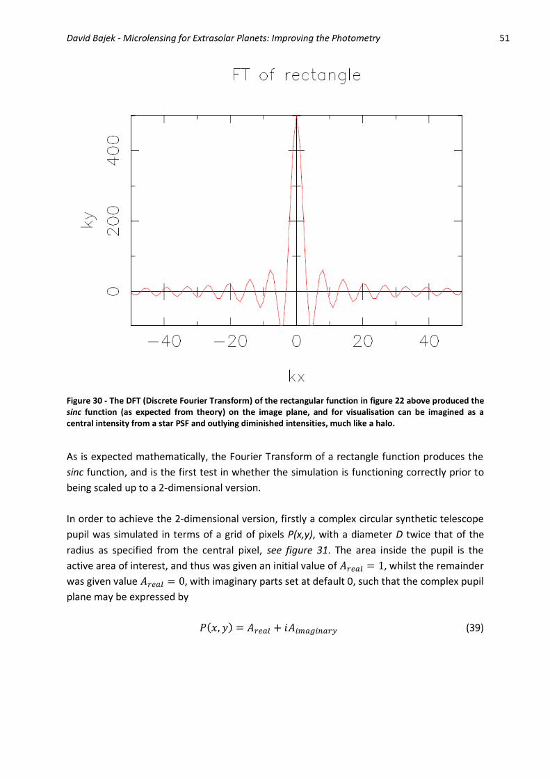
David Bajek - Microlensing for Extrasolar Planets: Improving the Photometry 51
Figure 30 - The DFT (Discrete Fourier Transform) of the rectangular function in figure 22 above produced the sinc function (as expected from theory) on the image plane, and for visualisation can be imagined as a central intensity from a star PSF and outlying diminished intensities, much like a halo.
As is expected mathematically, the Fourier Transform of a rectangle function produces the
sinc function, and is the first test in whether the simulation is functioning correctly prior to
being scaled up to a 2-dimensional version.
In order to achieve the 2-dimensional version, firstly a complex circular synthetic telescope
pupil was simulated in terms of a grid of pixels P(x,y), with a diameter D twice that of the
radius as specified from the central pixel, see figure 31. The area inside the pupil is the
active area of interest, and thus was given an initial value of , whilst the remainder
was given value , with imaginary parts set at default 0, such that the complex pupil
plane may be expressed by
(39)

David Bajek - Microlensing for Extrasolar Planets: Improving the Photometry 52
Figure 31 - The original complex 2-dimensional simulation of a telescope Pupil set up as a grid P(x,y) of pixels. The circular pupil is given an initial 'intensity' value of 1 to represent the light incoming from a distant star (black), whilst the remainder is set to 0 (ie where light is not gathered by the pupil, white).
A Fourier Transform was then carried out over the entire pupil grid A(x,y) similarly to that of
the rectangular function, to produce the resultant image on the new corresponding image
plane with brightness B(kx,ky) such that in general,
(40)
The image plane was then plotted similarly in an image pixel grid, see figure 32, where
highlighted profile slices were taken at several intervals from the radius in order to
investigate the nature of the resultant function.

David Bajek - Microlensing for Extrasolar Planets: Improving the Photometry 53
Figure 32 - The Fourier Transform from the circular aperture results in an Airy Function with a bright centre and airy rings of diminishing intensity. Three profiles slices are highlighted from the centre in order to investigate the function, see figure 33. Note, the greyscale colours of the PSF have been inverted and enhanced in order to emphasise the repeating Airy pattern.
As demonstrated, for monochromatic light of wavelength λ incident on a circular pupil of
diameter D, the 'perfect' PSF is an Airy function with a width λ/D shown as rings of
diminishing intensity from the central peak. The profile slices at the highlighted positions
were then plotted for confirmation into the varying intensity, see figure 33, indicating that
as with the 1-dimensional case, the simulation is indeed functioning correctly, and ready to
be developed further given sound theoretical foundations. Note that the profile slices from
the 2D Fourier Transform are mathematically equivalent to the square of the sinc function
produced by the 1D Fourier Transform.

David Bajek - Microlensing for Extrasolar Planets: Improving the Photometry 54
Figure 33 - The 1-dimensional Profile slices of the Fourier Transform reveal that the radial intensities
diminish as expected in a typical Airy Pattern, with a peak intensity at the centre, and is theoretically
comparable to the square of the sinc function generated from the DFT of the rectangular function.
Given that the aim of the simulation is to recreate a realistic image as seen by a true
telescope, another addition to the process is to consider another limitation of a typical
reflecting telescope - that is the effect of the secondary mirror, see figure 34, on the
resultant PSF.
Figure 34 - Diagram of a typical Newtonian Reflecting Telescope, where a secondary mirror redirects the light into the eyepiece, however it also serves as an obscuration as it blocks the initial incoming light in its path, leading to deviations in the resultant image. Diagram adapted from LCOGT.net[42]
Light Rays Entering the Telescope
Eyepiece
Profile Slices from Fourier Transform

David Bajek - Microlensing for Extrasolar Planets: Improving the Photometry 55
In order to simulate this effect, an exaggerated (for illustrative purposes) circular
obscuration representing the secondary mirror was placed in the pupil grid prior to the
Fourier Transform to result in the new image. A further implementation was to include
physical 'supports' for the mirror in the form of thin beams representing typical wires which
hold the mirror in place, once again greatly exaggerated for demonstrative effect of the
resultant PSF. See figures 35 - 37.
Figure 35 - Left, the original Pupil grid is Fourier Transformed to result in the PSF on the image grid, right, which is a centrally intense Airy Disk (this greyscale has not been altered).
Figure 36 - Left, an exaggerated obscuration representing the secondary reflecting mirror of the telescope is placed in the pupil plane, whose Fourier Transform results in the more pronounced Airy Pattern, right, with a notable ring shape outside of the central intensity.

David Bajek - Microlensing for Extrasolar Planets: Improving the Photometry 56
Figure 37 - Left, in addition to the secondary mirror, further obscurations representing the mirror's physical supports are added, the result of which is a further disrupted PSF, right, due to the square shape of the supports.
In addition to the obscuration, a single-case linear phase ramp was introduced across the
pupil, which occurs because the time-dependent change of arrival position for speckles will
cause a shift in the pattern, and thus the offset is the first basic approximation for a one-
time atmospheric shift. That is to say the star is not statically at the same position, but
rather changes its effective position with respect to the pupil, due to seeing factors.
For the complex amplitude A of the pupil plane, the Fourier Transform to the image plane
with brightness B has a phase such that
Where the linear phase ramp may be written as the dot product of the wavevector k in the
pupil plane and the position vector x in the pupil plane
The PSF will then shift in the image plane (without further distortion) proportionally to the
wavevector k, see figure 38.

David Bajek - Microlensing for Extrasolar Planets: Improving the Photometry 57
Figure 38 - Including a phase ramp in the simulation results in a shift in the PSF's position without affecting the overall shape, owing to the time-dependant change of the arrival position for the speckles.
Given the inherently random nature of atmospheric turbulence, the next step of the
simulation is to scale up the above effect and randomise the phase ramp (leading to a
random position of the PSF), as well as to include the speckling effect that results in the
constant changes of refractive index throughout the atmosphere. Following the
reconstruction of the obscuration of the secondary mirror to a more realistic (smaller) one,
this is achieved by applying a further 2-dimensional grid to the Fourier Transform from the
pupil plane of randomised Gaussian numbers.
The brightness level B of the image may now be given by the Fourier Transform of the pupil
P with respect to some amplitude A and some phase
Where the phase is given by
And where
Where C and S represent the 2D Random Gaussian grids required for the phase component,
with mean µ = 0 and variance σ2, giving
,

David Bajek - Microlensing for Extrasolar Planets: Improving the Photometry 58
And similarly, the Amplitude A may now be defined as
Where
And where CA and SA represent the 2D Random Gaussian grids required for the Amplitude
component, also with mean µ = 0 and variance σ2, giving
,
These random numbers govern a random change to the intensity of each pixel, resulting in
distortion of the entire image, the extent of which is dependent on the standard deviation in
the Gaussian distribution - that is, the spread and extent of the speckling will increase with
increasing standard deviation, see figure 39.

David Bajek - Microlensing for Extrasolar Planets: Improving the Photometry 59
Figure 39 - From a to d: Demonstrating the effects on the resulting image plane of increasing the standard deviation of the Gaussian Random Numbers which represent the atmospheric changes; increasing the standard deviation (spread) of the numbers increases the randomised changes in intensity, and results in increased speckling of the image.
a b
c d

David Bajek - Microlensing for Extrasolar Planets: Improving the Photometry 60
Note therefore that the image of figure 39a represents that which would be expected with
no randomised atmospheric turbulence at all, i.e. when the standard deviation in the
random Gaussian numbers is 0, or equivalent to purely diffraction-limited photometry.
The most realistic standard deviation σ (or variance, σ2) of the Gaussian distribution is
adapted from the work on the so-called Kolmogorov Model which was developed by
Tatarski[44] based on the initial investigations on turbulence by Kolmogorov[43]. The model
includes the power exponent 5/3 which is determined as the typical value for the
Kolmogorov model of typical atmospheric conditions[35] as discussed in section 3.3.2 above.
(41)
Where r0 is the Fried Seeing Parameter[44], which is a measure of the optical quality of the
atmosphere given in centimetres. This is to correspond directly with the aperture diameter
D of the telescope, and thus gives a measure of the extent of turbulence and whether this
will be comparable with seeing-limited or diffraction-limited observations; typical values of
the Fried parameter are 10cm for average seeing (as used in this simulation) and 20-40cm
for very good seeing conditions.
An approximate lucky imaging technique may now be adopted whereby for each image, the
random turbulence changes slightly, representing the sub-second exposure time typical of
each lucky image. The next step after taking several exposures is to stack them on the
brightest pixel, where increasing the number of original exposures in the stack will gradually
converge on an image which could potentially appear to have not been affected by
atmospheric turbulence, see figures 40 and 41.

David Bajek - Microlensing for Extrasolar Planets: Improving the Photometry 61
Figure 40 - From a to d: The effects of increasing the number of exposures (5, 20, 100 and 1000 respectively) which are stacked to produce the resultant images. The new PSFs are visibly smoother, and the speckling effect has been reduced as a result of stacking the randomised raised and lowered intensities of the turbulence effects. This has effectively reconstructed an approximation to the 'true' PSF which may be expected in diffraction-limited photometry (i.e. photometry from space) and is comparable to the original image produced in figure 39a before adding the turbulence effects. The red lines represent the profile slice taken for use in figure 41.
c
a b
d
5-image Stack
1000-image Stack 100-image Stack
20-image Stack

David Bajek - Microlensing for Extrasolar Planets: Improving the Photometry 62
Figure 41 - From a to d: The profile slices of the respective simulated images produced in figure 40 illustrate that an increase in exposures used in the stack converge on a reasonable approximation to that of a diffraction-limited image, such as that seen in the airy profile in figure 33.
The results clearly indicate that very short exposures which are stacked in this way can
reduce the effects of atmospheric turbulence, and with an increase of stacked images
converge on an approximation of diffraction-limited photometry. As a result, the simulation
is now primed to accept and process the Fourier Transform from any type of pupil plane to
an image plane, with customisable seeing conditions (i.e. ranging from very good to very
poor seeing), as well as stacking a custom number of exposures to lead to the final lucky
image.
d c
a b 5-image Stack
1000-image Stack 100-image Stack
20-image Stack

David Bajek - Microlensing for Extrasolar Planets: Improving the Photometry 63
3.3.4 Limitations & Future Expansion of the Simulation
Whilst the basis of the simulation is operational and the functions are customisable, a
number of improvements should be considered for its future use.
Firstly, as outlined in the theory above, the stacking process of lucky images does not
typically involve all exposures produced, only the highest 1-10% quality, where the quality is
selected based on the Strehl Ratio, which may be measured based on the resultant point-
spread functions.
Secondly, a mathematical analysis of the simulated lucky images should be carried out,
whereby simulated 2-dimensional lucky PSFs outlined in section 3.3.2 may be constructed
and compared with the simulated lucky exposures. This would involve developing pixel grids
of 2-dimensional PSFs with various core and halo distributions, such as Gaussian, Moffat or
as studied, the Lucky MofGau with a Moffat halo and a Gaussian core.
An MCMC algorithm may compare the simulated lucky images for example by a Chi-Squared
fit, and answer definitively which type of core/halo arrangement is realistic. Finally, using
real lucky images, the same analysis may be carried out, and further compared with the
synthetic lucky images in order to have both a practical and theoretical basis of the potential
improvements of lucky imaging.

David Bajek - Microlensing for Extrasolar Planets: Improving the Photometry 64
4.0 Conclusions
Whilst constantly developing upon the modelling techniques used for gravitational
microlensing events is vital, so too is selecting the highest quality subset of the available
data (magnification images) for reduction before being used in the modelling process.
Subsequently, even more important is the gathering of the raw data itself. There is huge
potential in adapting the lucky imaging technique in microlensing photometry in order to
ensure the best models are fit to the best selection of quality data, and thus analyse more
precisely the characteristics of detected extrasolar planets. The mathematical results
indicate a significant improvement in lucky imaging Signal to Noise Ratio over standard
imaging, and is therefore worth further continued analysis and exploration in order to
determine precisely the realistic improvement.
This is further confirmed by an early-stage simulation of the lucky imaging process, which
has illustrated that stacking sub-second lucky exposures is capable of reducing the speckling
effect which occurs due to atmospheric turbulence, essentially producing images which are
indeed potentially comparable to diffraction-limited photometry.
In conclusion, a quantitative investigation into increasing the quality of the original
photometric data available from any gravitational microlensing event demonstrates that
'lucky imaging' can lead to a marked improvement in the signal to noise ratio over that of
standard imaging techniques. The improvement to the original images obtained by lucky
imaging, together with critical sub-selection of images in the reductions process, leading to
improved simulations and model-fitting has the potential of resulting in more accurate
analysis, and thus may lead to the calculation of more accurate planetary parameters, as
well as the detection and confirmation of otherwise more difficult planetary candidates.

David Bajek - Microlensing for Extrasolar Planets: Improving the Photometry 65
5.0 Future Work
5.1 Constraints on Microlensed Systems using Lucky Imaging
Several important constraints may be placed on a microlensed system such as the planet
and star mass, by high resolution imaging several years after the event in order to detect
the star flux, colour and proper motion. There is immense interest in continuing some
themes outlined above, including testing the lucky imaging technique on appropriate
events, where an astrometric colour shift may be seen after several years. This could then
extend to looking at all planets discovered so far and making the relevant calculations when
revisiting them; given that lens and source stars come from different populations and
different masses, they inherently have different colours, and so taking images of the
microlensing events several years later with lucky imaging using two filters, one may expect
to see the change in position and investigate important constraints for the system which
could begin with estimates from the FTS/FTN lucky imagers in the very near future. Lucky
imaging would be essential here given the precise and delicate nature of the calculations
required for astrometry, where lucky imaging gives the best chance of high quality
photometry with minimal atmospheric interference.
5.2 Observing
One highly anticipated and beneficial aspect of undertaking a project in microlensing is the
invitation to take part in observing runs during each season. Particularly interesting and
unique events such as planetary candidates often feature in typical astronomy theses, and
dependant on their rarity may lead to further, more intensive investigations. I was invited to
complete the following workloads:
- 2 weeks observing with the Danish 1.54m telescope[45] at La Silla, Chile
The Danish telescope is operated in person on site, the first week of which is spent under
the training of an experienced observer, and the following week is spent training the next
observer on site.
- 1 week remote observing with MONET 1.2m telescope[46] at SAAO, South Africa
The MONET telescope is operated remotely in a semi-automatic manner, which requires a
remote observer to start up, monitor the semi-automatic microlensing observations fed to
the telescope via ARTEMiS[47], obtain calibrations, and shut down the telescope following an
observing night.
In addition to the practical knowledge and understanding gained through such intense
astronomical observing at La Silla and SAAO, the work itself also allows membership of the
MiNDSTEp Consortium[48] for that year. Members are entitled to co-author papers which
result from the observations collected during that period, where typically one year of
membership will give rise to co-authorship of 5 or more peer-reviewed scientific papers.

David Bajek - Microlensing for Extrasolar Planets: Improving the Photometry 66
6.0 Publications
This section contains summarised information regarding any publications, having been
submitted or currently in draft, on which I have co-authorship and which have been
completed in connection with Gravitational Microlensing during this Project. Many aspects
of the computational or mathematical theory outlined in this thesis are often used to
complete scientific papers such as these, with many groups around the world collaborating
and sharing data and expertise in order to contribute towards various sections within.
"Microlensing Binaries with Brown Dwarf Companions" (Submitted August 2012); I. -G.
Shin, C. Han, A. Gould and others including D. Bajek[49]
An investigation of microlensing events which have been identified as binary systems
containing brown dwarf companions; objects with masses between that of large gas giant
planets and low-mass stars. Of seven candidate events selected for analysis, two have been
confirmed to contain such brown dwarfs.
"MOA-2010-BLG-073Lb: A Cool, Low Mass Brown Dwarf Orbiting an M-Dwarf" (Accepted
by ApJ November 2012): R.A. Street, J.-Y Choi, Y. Tsapras, C. Han and others including D.
Bajek
This paper also discusses an event which includes a brown dwarf, but was of particular
interest as the source star of the event had previously been known to be photometrically
variable, however the investigation indicates that the source is actually an irregular variable
and is a red giant.
"A Cool Jupiter-Mass Planet in Microlensing Beyond the Snow Line in Event OGLE-2011-
BLG-0251" (Submitted to A&A, October 2012); N. Kains, R. Street, C. Han, A. Udalski and
others including D. Bajek
This paper discusses the discovery of a Jupiter-mass planet in a microlensing event, and
outlines the techniques used to determine its characteristics, and establish the separation
from its host star, which is beyond the snow line. Given the rarity of planets discovered by
the microlensing technique, publications of all occurrences are vital in drawing
collaborations to assist in the complex nature of their analysis.
"Photometric Potential of Lucky Imaging"; (In Draft), K. Horne, D. Bajek, K. Harpsoe
As outlined in section 3.0, a theoretical investigation into the benefit of lucky imaging
photometry over standard imaging photometry. This includes the potential numerical
improvement in the sound to noise under various circumstances, and the results of a
simulation demonstrating the lucky imaging technique.

David Bajek - Microlensing for Extrasolar Planets: Improving the Photometry 67
7.0 References
[1] Wolszczan, A., Frail, D. (1992). "A planetary system around the millisecond pulsar
PSR1257 + 12". Nature 355 (6356): 145–147.
[2] Schneider, Jean "Interactive Extra-solar Planets Catalog". The Extrasolar Planets
Encyclopedia
[3] http://en.wikipedia.org/wiki/Extrasolar_planet
[4] G. Chauvin; A.M. Lagrange; C. Dumas; B. Zuckerman; D. Mouillet; I. Song; J.-L. Beuzit; P.
Lowrance (2004). "A giant planet candidate near a young brown dwarf". Astronomy &
Astrophysics 425 (2): L29 – L32
[5] D.J. Erskine, J. Edelstein, D. Harbeck and J. Lloyd (2005). "Externally Dispersed
Interferometry for Planetary Studies". In Daniel R. Coulter. Proceedings of SPIE: Techniques
and Instrumentation for Detection of Exoplanets II. 5905. pp. 249–2
[6] Hidas, M. G.; Ashley, M. C. B.; Webb, et al. (2005). "The University of New South Wales
Extrasolar Planet Search: methods and first results from a field centred on NGC 6633".
Monthly Notices of the Royal Astronomical Society 360 (2): 703–717
[7] Benedict et al.; McArthur, B. E.; Forveille, T.; Delfosse, X.; Nelan, E.; Butler, R. P.;
Spiesman, W.; Marcy, G. et al. (2002). "A Mass for the Extrasolar Planet Gliese 876b
Determined from Hubble Space Telescope Fine Guidance Sensor 3 Astrometry and High-
Precision Radial Velocities". The Astrophysical Journal Letters 581 (2): L115–L118
[8] http://www.esa.int/SPECIALS/Operations/SEMK5HZTIVE_0.html
[9] Einstein, Albert (1936). "Lens-like Action of a Star by the Deviation of Light in the
Gravitational Field". Science 84 (2188): 506–507
[10] Alcock, C. et al. (1993). "Possible gravitational microlensing of a star in the Large
Magellanic Cloud". Nature 365 (6447): 621–623
[11] http://wfirst.gsfc.nasa.gov/about
[12] Gould, A., 2000 "A Natural Formalism for Microlensing". The Astrophysical Journal 542
[13] Horne, K. et al (2009) "A metric and optimization scheme for microlens planet
searches" Monthly Notices of the Royal Astronomical Society, Vol. 396, No. 4., pp. 2087-
2102
[14] Paczyński, Bohdan (1996) "Gravitational microlensing in the Local Group", Annual
Review of Astronomy and Astrophysics, 34: 419
[15] Di Stefano, R. (2005) "Mesolensing Explorations of Nearby Masses: From Planets to
Black Holes", The Astrophysical Journal, V684, Issue 1: 59-67.
[16] Di Stefano, R. (2009) "New opportunities in microlensing and mesolensing" The
Astronomy and Astrophysics Decadal Survey, Science White Papers, no. 65
[17] Di Stefano, R., & Night, C. (2008) "Discovery and Study of Nearby Habitable Planets
with Mesolensing" Harvard-Smithsonian Center for Astrophysics.
[18] Lepine, S. & Di Stefano, R. (2012) "On the detectability of a predicted mesolensing even
associated with the high proper motion star VB 10" ApJ 749 L6

David Bajek - Microlensing for Extrasolar Planets: Improving the Photometry 68
[19] Di Stefano, R. et al (2012) "Searching for Planets During Predicted Mesolensing Events:
Theory, and the Case of VB 10" arXiv:1202.5314v1
[20] http://en.wikipedia.org/wiki/Rogue_planet
[21] Sumi, T., Kamiya, K., Bennett, D. P., et al. (2011) "Unbound or distant planetary mass
population detected by Gravitational Microlensing" 2011, Nature, 473, 349
[22] Quanz, S. P. et al (2012) "Direct imaging constraints on planet populations detected by
microlensing" arXiv:1203.3647v1
[23] Veras, D., & Raymond, S. N. (2012), "Planet-planet scattering alone cannot explain the
free-floating planet population" arXiv:1201.2175
[24] Stevenson, D.J. (1998) "Possibility of Life-sustaining Planets in Interstellar Space"
Nature 400, 32
[25] Lissauer, J.J., (1987) "Timescales for Planetary Accretion and the Structure of the Proto-
planetary disk" Icarus 69: 249–265
[26] Abbot, D.S. & Switzer, E.R (2011) "The Steppenwolf: A proposal for a habitable planet in
interstellar space"arXiv:1102.1108v2
[27] Baross, J. A., and Hoffman, S. E. 1985, Origin of Life, 15, 327
[28] Debes, J.H & Sigurdson, S. (2007) "The Survival Rate of Ejected Terrestrial Planets with
Moons" arXiv:0709.0945v1
[29] John Archibald Wheeler, "The 'Past' and the 'Delayed-Choice' Double-Slit Experiment",
in Mathematical Foundations of Quantum Theory, edited by A.R. Marlow, p. 13
[30] http://www.space.com/529-quantum-astronomy-double-slit-experiment.html
[31] Jacques, Vincent; et al. (2007). "Experimental Realization of Wheeler's Delayed-Choice
Gedanken Experiment". Science 315: 966–968
[32] Dominik, M., et al. 2007, MNRAS, 380, 792
[33] http://ogle.astrouw.edu.pl/ogle4/ews/2011/ews.html
[34] TATARSKI, V. I. (1961). "Wave Propagation in a Turbulent Medium", McGraw-Hill Books
[35] Tubbs, R. N., (2003) "Lucky Exposures: Diffraction limited astronomical imaging through
the atmosphere", Cambridge University
[36] Fried, D. (1978). "Probability of getting a lucky short-exposure image through
turbulence". Optical Society of America 68 (12): 1651–1658
[37] Fried, D. (1966). "Optical Resolution Through a Randomly Inhomogeneous Medium for
Very Long and Very Short Exposures". Optical Society of America Journal 56 (10): 1372
[38] Strehl, K. (1895),"Aplanatische und fehlerhafte Abbildung im Fernrohr", Zeitschrift für
Instrumentenkunde, 362-370
[39] Moffat, A.F.J. (1969) "A Theoretical Investigation of Focal Stellar Images in the
Photographic Emulsion and Application to Photographic Photometry" Astronomy and
Astrophysics, Vol. 3, p. 455 (1969)
[40] Baldwin, J.E. (2008) "The point spread function in Lucky Imaging and variations in seeing
on short timescales" A&A 480, p589–597

David Bajek - Microlensing for Extrasolar Planets: Improving the Photometry 69
[41] Woodward, P. M.; Davies, I. L. (1952). "Information theory and inverse probability in
telecommunication". Proceedings of the IEE - Part III: Radio and Communication Engineering
99 (58): 37–44
[42] http://lcogt.net/spacebook/reflecting-telescopes
[43] Kolmogorov, A. N. (1941) "The local structure of turbulence in incompressible viscous
fluid for very large Reynolds numbers". Proceedings of the USSR Academy of Sciences 30:
299–303
[44] Fried, D. L. (1966). "Optical Resolution Through a Randomly Inhomogeneous Medium
for Very Long and Very Short Exposures". Journal of the Optical Society of America 56 (10):
1372–1379
[45] http://www.eso.org/public/teles-instr/lasilla/danish154.html
[46] http://monet.uni-goettingen.de/foswiki
[47] http://www.artemis-uk.org/
[48] http://www.mindstep-science.org/
[49] "Microlensing Binaries with Brown Dwarf Companions" (2012); I. -G. Shin, C. Han, A.
Gould et al, arXiv:1208.2323v1
[50] G. Chauvin, A.-M. Lagrange, C. Dumas, B. Zuckerman, D. Mouillet, I. Song, J.-L. Beuzit, P.
Lowrance (2004) “A giant planet candidate near a young brown dwarf” Direct VLT/NACO
observations using IR wavefront sensing, Astronomy and Astrophysics 425, pp. L29–L32
[51] D. Bennett, I. Bond et al (2004), “The Microlensing Planet Finder: Completing the
Census of Extrasolar Planets in the Milky Way”, Proceedings of the SPIE Astronomical
Telescopes and Instrumentation Symposium
[52] D. Bennet, J. Anderson et al (2010) “Completing the Census of Exoplanets with
Microlensing Planet Finder (MPF)”, arXiv:1012.4486v1
[53] http://www.iau.org
[54] Y. Tsapras, R. Street, K. Horne et al (2009), “RoboNet-II: Follow-up observations of
microlensing events with a robotic network of telescopes” Astronomische Nachrichten,
Vol.330, Issue 1, p.4
[55] C. Snodgrass, Y. Tsapras, R. Street et al (2008), “The web-PLOP observation
prioritisation system”, PoS(GMC8)056
[56] D. M. Bramich (2008), “A New Algorithm for Difference Image Analysis”,
arXiv:0802.1273v1
[57] Bond, I. A. et al. (2004). "OGLE 2003-BLG-235/MOA 2003-BLG-53: A Planetary Microlensing Event". The Astrophysical Journal Letters 606 (2): L155–L158. arXiv:astro-ph/0404309