dating the timeline of financial bubbles during the subprime...
TRANSCRIPT

DATING THE TIMELINE OF FINANCIAL BUBBLES DURING THE SUBPRIME CRISIS
BY
Peter C.B. Phillips and Jun Yu
COWLES FOUNDATION PAPER NO. 1348
COWLES FOUNDATION FOR RESEARCH IN ECONOMICS YALE UNIVERSITY
Box 208281 New Haven, Connecticut 06520-8281
2012
http://cowles.econ.yale.edu/

Quantitative Economics 2 (2011), 455–491 1759-7331/20110455
Dating the timeline of financial bubbles during thesubprime crisis
Peter C. B. PhillipsYale University, University of Auckland, University of Southampton, and
Singapore Management University
Jun YuSingapore Management University
A new recursive regression methodology is introduced to analyze the bubble char-acteristics of various financial time series during the subprime crisis. The meth-ods modify a technique proposed in Phillips, Wu, and Yu (2011) and provide atechnology for identifying bubble behavior with consistent dating of their origi-nation and collapse. The tests serve as an early warning diagnostic of bubble ac-tivity and a new procedure is introduced for testing bubble migration across mar-kets. Three relevant financial series are investigated, including a financial assetprice (a house price index), a commodity price (the crude oil price), and one bondprice (the spread between Baa and Aaa). Statistically significant bubble character-istics are found in all of these series. The empirical estimates of the originationand collapse dates suggest a migration mechanism among the financial variables.A bubble emerged in the real estate market in February 2002. After the subprimecrisis erupted in 2007, the phenomenon migrated selectively into the commoditymarket and the bond market, creating bubbles which subsequently burst at theend of 2008, just as the effects on the real economy and economic growth becamemanifest. Our empirical estimates of the origination and collapse dates and testsof migration across markets match well with the general dateline of the crisis putforward in the recent study by Caballero, Farhi, and Gourinchas (2008a).
Keywords. Financial bubbles, crashes, date stamping, explosive behavior, migra-tion, mildly explosive process, subprime crisis, timeline.
JEL classification. C15, G01, G12.
Peter C. B. Phillips: [email protected] Yu: [email protected] acknowledges support from the NSF under Grants SES 06-47086 and SES 09-56687. Yu acknowl-edges support from the Singapore Ministry of Education AcRF Tier 2 fund under Grant T206B4301-RS. Wewish to thank a co-editor, three anonymous referees, seminar participants in many universities, the 2010International Symposium on Econometric Theory and Applications held at Singapore Management Uni-versity, the World Congress of the Econometric Society in Shanghai, the second Singapore Conference onQuantitative Finance at Saw Centre for Quantitative Finance, the Workshop on Econometric and FinancialStudies After Crisis at Academia Sinica, the 2011 Shanghai Econometrics Workshop, and the Frontiers inFinancial Econometrics Workshop for helpful comments.
Copyright © 2011 Peter C. B. Phillips and Jun Yu. Licensed under the Creative Commons Attribution-NonCommercial License 3.0. Available at http://www.qeconomics.org.DOI: 10.3982/QE82

456 Phillips and Yu Quantitative Economics 2 (2011)
There is a very real danger, fellow citizens, that the Icelandic economy in the worst casecould be sucked into the whirlpool, and the result could be national bankruptcy (PrimeMinister Geir Haarde, televised address to Icelandic Nation, October 8, 2008).
Between 40 and 45 percent of the world’s wealth has been destroyed in little less than a yearand a half (Stephen Schwarzman, March 11, 2009).
Federal Reserve policymakers should deepen their understanding about how to combatspeculative bubbles to reduce the chances of another financial crisis (Donald Kohn, Fed-eral Reserve Board Vice Chairman, March 24, 2010).
1. Introduction
Financial bubbles have been a longstanding topic of interest for economists, involv-ing both theorists and empirical researchers. Some of the main issues have focused onmechanisms for modeling bubbles, reconciling bubble-like behavior in the context ofrational expectations of future earnings, mechanisms for detecting bubbles and mea-suring their extent, exploring causes and the psychology of investor behavior, and con-sidering suitable policy responses. While there is general agreement that financial bub-bles give rise to misallocation of resources and can have serious effects on real economicactivity, as yet there has been little consensus among economists and policy makers onhow to address the many issues raised above.
The global financial turmoil over 2008–2009, triggered by the subprime crisis in theUnited States and its subsequent effect on commodity markets, exchange rates, and realeconomic activity, has led to renewed interest among economists in financial bubblesand their potential global consequences. There is now widespread recognition amongpolicy makers as well as economists that changes in the global economy over the lastdecade, far from decoupling economic activity as was earlier believed, have led to pow-erful latent financial linkages that have increased risks in the event of a large commonshock. The magnitude of the crisis is so large, the mechanism so complex, and the con-sequences so important to the real economy that understanding the phenomenon, ex-ploring its causes, and mapping its evolution have presented major challenges to theeconomics profession. As the quotations that preface this article indicate, a substan-tial percentage of the world’s accrued wealth was destroyed within 18 months of thesubprime crisis, with manifold effects ranging from the collapse of major financial in-stitutions to the near bankruptcy of national economies. There is also recognition thatnew empirical methods are needed to improve understanding of speculative phenom-ena and to provide early warning diagnostics of financial bubbles.
The recent background of financial exuberance and collapse with concatenatingeffects across markets and nations provides a rich new environment for empirical re-search. The most urgent ongoing questions relate to matters of fiscal, monetary, andregulatory policies for securing financial stability and buttressing real economic activ-ity. Beyond these immediate policy issues are underlying questions relating to the emer-gence of the phenomenon and its evolutionary course through the financial and eco-nomic systems. It is these latter issues that form the focus of interest of the present pa-per.

Quantitative Economics 2 (2011) Timeline of financial bubbles 457
The subprime crisis is not an isolated empirical event. In a recent article, Caballero,Farhi, and Gourinchas (CFG) (2008a) argued that the Internet bubble in the 1990s, theasset bubbles over 2005–2006, the subprime crisis in 2007, and the commodity bubblesof 2008 are all closely related. CFG go further and put forward a sequential hypothesisconcerning bubble creation and collapse that accounts for the course of the financialturmoil in the U.S. economy using a simple general equilibrium model without mone-tary factors, but with goods that may be partially securitized. Date-stamping the time-line of the origination and collapse of the various bubbles is a critical element in thevalidity of this sequential hypothesis. Empirical evaluation further requires some econo-metric technology for testing the presence of bubble migration across markets.
The present paper uses econometric methodology to test if and when bubblesemerged and collapsed in the real estate market, the commodity market, and the bondmarket over the period surrounding the subprime crisis. New econometric methods areintroduced for testing bubble migration across markets. Several series are studied. Inparticular, we investigate the bubble characteristics in the U.S. house price index fromJanuary 1990 to January 2009, the price of crude oil from January 1999 to January 2009,and the spread between Baa and Aaa bond rates from January 3, 2006 to July 2, 2009.Figure 1 shows time series plots of the three series. Our methods enable us to determinewhether a bubble emerged in each series, to date-stamp the origination in that event,and correspondingly to assess whether the bubble collapsed and the date of that col-lapse. The empirical date stamps so determined are then matched against the hypothe-sized sequence of events described in the model of CFG.
The econometric methods used here are closely related to those proposed in Phillips,Wu, and Yu (2011; PWY hereafter). In particular, the methods rely on forward recursiveregressions coupled with sequential right-sided unit root tests. The sequential tests as-sess period by period evidence for unit root behavior against mildly explosive alterna-tives. Mildly explosive behavior can be modeled by an autoregressive process with a root(ρ) that exceeds unity but that is still in the general vicinity of unity. Phillips and Mag-dalinos (PM) (2007a, 2007b) showed that this “mildly explosive” vicinity of unity can besuccessfully modeled in terms of deviations of the form ρ − 1 = c/kn > 0, where c is apositive constant and kn is a sequence that passes to infinity with, but more slowly than,the sample size n, so that ρ → 1. These processes therefore involve only mild depar-tures from strict (rational) martingale behavior in markets. They include submartingaleprocesses of the type that have been used to model rational bubble behavior in finance(Evans (1991), Campbell, Lo, and McKinley (1997)). PM (2007a, 2007b) have investigatedthis class of process, developed a large sample asymptotic theory, and shown that thesemodels are amenable to econometric inference, unlike purely explosive processes forwhich no central limit theory is applicable.
PWY applied forward recursive regression methods to Nasdaq stock prices duringthe 1990s, and using sequential tests against mildly explosive alternatives were able todate-stamp the origination of financial exuberance in the Nasdaq market to mid-1995,prior to the famous remark of Alan Greenspan in December 1996 about irrational ex-uberance in financial markets. This test therefore revealed that there was anticipatoryempirical evidence supporting mildly explosive behavior in stock prices over a year prior

458 Phillips and Yu Quantitative Economics 2 (2011)
(a) House Prices (b) Oil Price
(c) Bond Price
Figure 1. Time series plots of real prices for three financial assets: (a) monthly observations ofthe house price index from January 1990 to January 2009 adjusted by rental; (b) monthly obser-vations of crude oil prices adjusted by supply; and (c) daily observations of the spread betweenBaa bond rates and Aaa bond rates from January 3, 2006 to July 2, 2009. The estimated bubbleorigination and collapse dates are also shown on the figures.
to Greenspan’s remarks. In ongoing work, Phillips and Yu (2009) and Phillips, Shi, andYu (2011) developed a limit theory for this date stamping technology, explored multiplebubble detection, and checked the finite sample capability of the procedure to identifyand date bubble behavior. The date stamp estimators were shown to be consistent forthe origination and collapse of bubble behavior and the dating mechanism was shownto work well in finite samples.
We use this methodology to explore the sequential pattern of events of the currentfinancial crisis. Dating helps to characterize the phenomenon by identifying the individ-ual events and by fixing their extent and sequencing. It may be viewed as a first step inunderstanding the phenomenon and in searching for causes of the behavioral changesinvolved in bubble origination and collapse. Date stamping in conjunction with migra-tion analysis assists in evaluating hypotheses about the concatenation of bubble activityover time and across markets, such as those developed by CFG. The forward recursiveregression approach used here enables early identification of the appearance of mildlyexplosive behavior in asset prices, thereby providing anticipatory evidence of a (local)

Quantitative Economics 2 (2011) Timeline of financial bubbles 459
move away from martingale behavior. This evidence can be used as an early warning di-agnostic of (financial) exuberance, and thereby can assist policy makers in surveillanceand regulatory actions, as urged by Fed Vice Chairman Donald Kohn in one of the open-ing quotes of this article. Similarly, the approach helps to identify a subsequent switchback to martingale behavior as explosive sentiment collapses.
Empirical evidence of emergent mildly explosive behavior is found in all of the timeseries studied here, and in all of them that manifest mildly explosive behavior, there isfurther evidence of subsequent collapse. Figure 1 shows the origination and collapsedates for the bubbles identified in the three financial time series mentioned earlier.For the real estate market, the bubbles emerged prior to the subprime crisis. For theother series, the bubbles all emerged after the subprime crisis. These findings reveal asequence of mildly explosive events, each followed by a financial collapse that corrobo-rates the sequential hypothesis given by CFG. Consideration of a wider group of relatedfinancial series following the eruption of the subprime crisis indicates that bubbles ofthe type found in the series in Figure 1 are not always evident in other commodities. Ac-cordingly, the empirical evidence supports a selective migration of the bubble activitythrough financial markets as the subprime crisis evolved and liquid funds searched forsafe havens.
The present paper differs from PWY in three aspects. The first difference involves thetreatment of initialization. In PWY, the initial condition is fixed to be the first observa-tion in the full sample, whereas in this paper, the initial observation is selected basedon an information criterion. The use of information criteria in the selection of the initialobservation allows for sharper identification of the bubble origination date. As a result,when a long series is available, the new method may not necessarily use all the obser-vations to identify the most recent bubble episode. Second, in this paper, a method fortesting bubble migration is developed, a limit theory for the new procedure is obtained,and the migration test is implemented in the empirical application. Finally, the empiri-cal focus of this paper is the subprime crisis and some of the events unfolding over theperiod 2002–2009.
The plan of the paper is as follows. Section 2 reviews the econometric methodologyfor dating bubble characteristics, discusses rational bubble and variable discount ratesources of financial exuberance, outlines some of the relevant facts concerning the sub-prime crisis, and relates the timeline implications of the theoretical results obtained inCFG (2008a). Section 3 describes the data that are used in the present empirical study.Section 4 presents the empirical findings and matches the estimates to the theory ofCFG (2008a). Section 5 concludes. New limit theory for the migration test is developedin the Appendix.
2. Bubbles, the subprime crisis, econometric dating, and bubble migration
2.1 Bubbles and crashes
In the popular press, the term “financial bubble” refers to a situation where the price of afinancial asset rapidly increases and does so in a speculative manner that is distinct fromwhat is considered to be the asset’s intrinsic value. The term carries the innuendo that

460 Phillips and Yu Quantitative Economics 2 (2011)
the increase is not justified by economic fundamentals and that there is, accordingly,risk of a subsequent collapse in which the asset price falls precipitously. In such cases,the bubble phenomenon is typically confirmed in retrospect.
A common definition that makes this usage precise is that bubble conditions arisewhen the price of an asset significantly exceeds the fundamental value that is deter-mined by the discounted expected value of the cash flows that ownership of the assetcan generate. However, discount rates may be variable and, as demonstrated below, thetime profile of the discount rate can have important effects on the characteristics of thefundamental price and may even propagate explosive price behavior.
An important secondary characteristic of the bubble phenomenon is that duringboth the run-up and run-down periods, the asset is subject to high volume trading inwhich the direction of change is widely anticipated (and relied upon), as distinct fromnormal market conditions in which the asset price follows a near martingale. It is thisdeviation from martingale behavior that provides a mechanism for identifying both theemergence of the boom phase of a bubble behavior and its subsequent crash.
This distinction is recognized in the rational bubble literature, which characterizesthe boom phase of a bubble in terms of explosive dynamics or submartingale behav-ior. This property contrasts with the efficient market martingale property, which impliesunit root time series dynamic behavior. To explain the difference in terms of the com-monly used present value model, let Pt be the stock price at time t before the dividendpayout, let Dt be the dividend payoff from the asset at time t, and let r be the discountrate (r > 0). The standard no arbitrage condition implies that
Pt = 11 + r
Et(Pt+1 +Dt+1) (1)
and recursive substitution yields
Pt = Ft +Bt� (2)
where Ft =∑∞i=1 (1 + r)−iEt(Dt+i) and
Et(Bt+1)= (1 + r)Bt� (3)
Hence, the asset price is decomposed into two components: a “fundamental” compo-nent, Ft , that is determined by expected future dividends, and a supplementary solutionthat corresponds to the “bubble” component, Bt .1 In the absence of bubble conditions,Pt = Ft . Otherwise, Pt = Ft +Bt and price embodies the explosive component Bt , whichsatisfies the submartingale property (3). Consequently, under bubble conditions, Pt willmanifest the explosive behavior inherent in Bt . This explosive property is very differentfrom the random wandering (or unit root) behavior that is present in Ft when Dt is amartingale and that is commonly found for asset prices in the empirical literature.
Over long periods of time, some asset prices like equities also tend to manifest em-pirical evidence of a drift component. Unit root time series with a drift can generate
1Extensions of the framework (1)–(3) to log linear approximations such as those in Campbell and Shiller(1988) and the validity of these approximations are considered in Lee and Phillips (2011).

Quantitative Economics 2 (2011) Timeline of financial bubbles 461
periods of run-up if the variance of the martingale component is small and the drift isstrong enough. But accumulated gains in such cases are at most of O(n) for sample sizen. In practice, of course, the drift component is usually small and is generally negligibleover short periods, so the unit root behavior is the dominant characteristic and clear ev-idence of gains only shows up over long horizons. On the other hand, the run-up ratein an explosive process is O((1 + r)n) for some r > 0, as in (3), and is therefore muchgreater. This difference between linear and exponential growth combined with the non-linear curvature in an explosive process are testable properties that distinguish the twoprocesses. In terms of model (1) and its solution (2), both Bt and Pt increase rapidlyduring the boom phase of the bubble according to Et(Bt+h) = (1 + r)hBt and the ini-tialization B0 > 0. But when the bubble conditions collapse and the particular solutiondisappears, then Pt = Ft , which corresponds to a sudden collapse in the asset price. Ifthe dividend process Dt follows a martingale, reflecting market conditions that gener-ate cash flows, then Ft is similarly a martingale and is cointegrated with Dt . Under suchconditions, the presence of an additional “rational bubble” submartingale componentBt in Pt can account for an explosive run-up in the asset price Pt .
Importantly, making the discount factor rt either stationary or integrated of order 1does not change our analysis qualitatively because the implications for the statisticalproperties of Ft , Bt , and Pt are the same as with the constant r. For example, if rt isstationary, (3) becomes
Et(Bt+1) = (1 + rt)Bt� (4)
Then if (3) is fitted, r = (∏T
t=1(1 + rt))1/T > 1, implying an explosive process for Bt and
hence Pt , even if Ft itself is not explosive.
2.2 The effects of a time varying discount rate
This paper interprets explosiveness in price as sufficient evidence for bubbles and thisinterpretation holds true under a variety of assumptions on the discount rate. As in-dicated above, certain time profiles for the discount rate can have an important effecton the characteristics of the fundamental price. The present section illustrates this pos-sibility by developing a simple propagating mechanism for explosive behavior in thefundamental price under a time varying discount rate.
If dividends grow at a constant rate rD with rD < r in (1),2 the fundamental value ofthe stock price is
Ft = Dt
r − rD� (5)
This is the well known Gordon growth model. It is evident that in this case the funda-mental value can be very sensitive to changes in r when r is close to rD. In fact, thefundamental value diverges as r ↘ rD, so that a price run-up is evidently possible under
2This assumption obviously violates the assumption we adopted earlier, namely, constancy, stationarity,or integration of order 1.
462 Phillips and Yu Quantitative Economics 2 (2011)
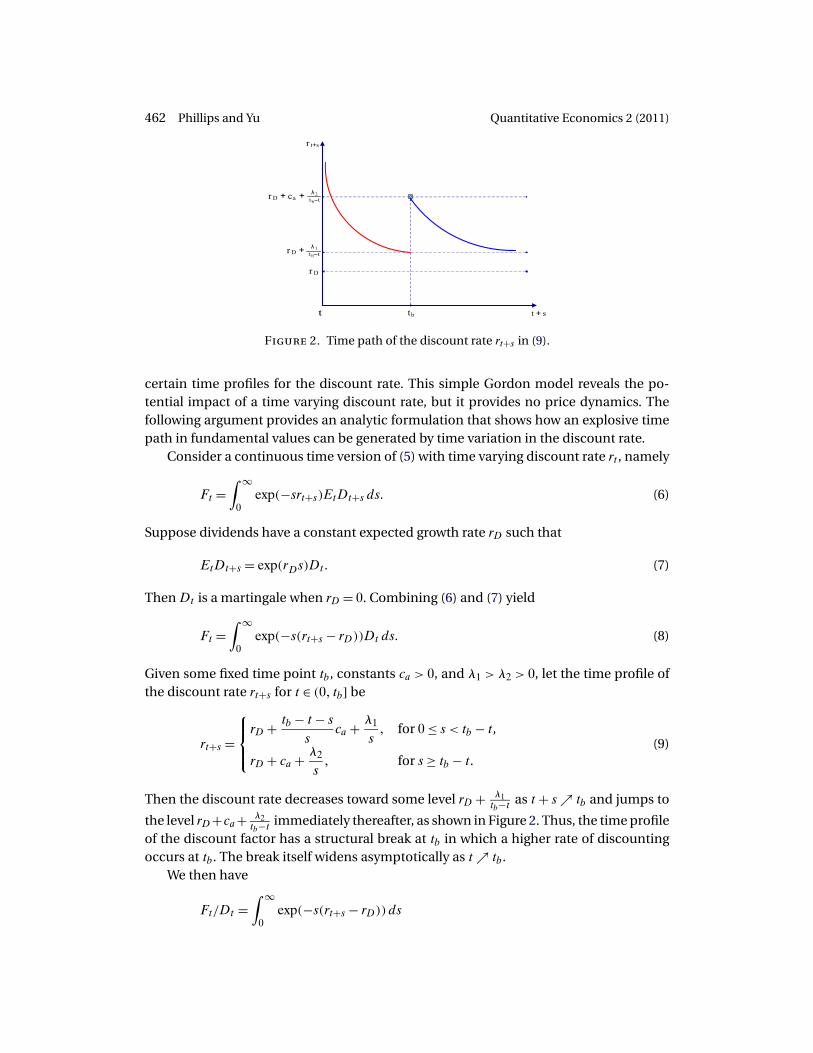
Figure 2. Time path of the discount rate rt+s in (9).
certain time profiles for the discount rate. This simple Gordon model reveals the po-tential impact of a time varying discount rate, but it provides no price dynamics. Thefollowing argument provides an analytic formulation that shows how an explosive timepath in fundamental values can be generated by time variation in the discount rate.
Consider a continuous time version of (5) with time varying discount rate rt , namely
Ft =∫ ∞
0exp(−srt+s)EtDt+s ds� (6)
Suppose dividends have a constant expected growth rate rD such that
EtDt+s = exp(rDs)Dt� (7)
Then Dt is a martingale when rD = 0. Combining (6) and (7) yield
Ft =∫ ∞
0exp(−s(rt+s − rD))Dt ds� (8)
Given some fixed time point tb, constants ca > 0, and λ1 > λ2 > 0, let the time profile ofthe discount rate rt+s for t ∈ (0� tb] be
rt+s =
⎧⎪⎨⎪⎩rD + tb − t − s
sca + λ1
s� for 0 ≤ s < tb − t,
rD + ca + λ2
s� for s ≥ tb − t.
(9)
Then the discount rate decreases toward some level rD + λ1tb−t as t + s ↗ tb and jumps to
the level rD+ca+ λ2tb−t immediately thereafter, as shown in Figure 2. Thus, the time profile
of the discount factor has a structural break at tb in which a higher rate of discountingoccurs at tb. The break itself widens asymptotically as t ↗ tb.
We then have
Ft/Dt =∫ ∞
0exp(−s(rt+s − rD))ds

Quantitative Economics 2 (2011) Timeline of financial bubbles 463
=∫ tb−t
0exp(−ca(tb − t − s)− λ1)ds +
∫ ∞
tb−texp(−cas − λ2)ds
= e−λ1
[e−ca(tb−t−s)
ca
]tb−t
0+ e−λ2
[e−cas
−ca
]∞
tb−t
= e−λ1
ca
[1 − e−ca(tb−t)
]+ e−λ2
cae−ca(tb−t)
= e−λ1
ca+ (e−λ2 − e−λ1)
cae−ca(tb−t) := σt
and the time path of Ft/Dt is explosive over t ∈ (0� tb]. Over this interval, Ft evolves ac-cording to the differential equation
dFt = (e−λ2 − e−λ1)e−ca(tb−t)Dt dt + σt dDt�
Since caFt/Dt = e−λ1 + (e−λ2 − e−λ1)e−ca(tb−t), we have
dFt = (e−λ2 − e−λ1)e−ca(tb−t)
e−λ1 + (e−λ2 − e−λ1)e−ca(tb−t)caFt dt + σt dDt for t ∈ (0� tb]�
For t close to tb, the generating mechanism for Ft is approximately
dFt = (e−λ2 − e−λ1)
e−λ1 + (e−λ2 − e−λ1)caFt dt + σt dDt
= {1 − e−(λ1−λ2)
}caFt dt + σt dDt�
which is an explosive diffusion because
cb = {1 − e−(λ1−λ2)
}ca > 0�
since ca > 0 and e−(λ1−λ2) < 1. The discrete time path of Ft in this neighborhood is there-fore propagated by an explosive autoregressive process with coefficient ρ = ecb > 1.
The heuristic explanation of this behavior is as follows. As t ↗ tb there is growing an-ticipation that the discount factor will soon increase. Under such conditions, investorsanticipate the present to become more important in valuing assets. This anticipationin turn leads to an inflation of current valuations and price fundamentals Ft becomeexplosive as this process continues.
On the other hand, for t > tb, we have
rt+s = rD + ca + λ2
sfor s > 0
and then
Ft
Dt=∫ ∞
0exp(−s(rt+s − rD))ds
=∫ ∞
0exp(−cas − λ2)ds
464 Phillips and Yu Quantitative Economics 2 (2011)
= e−λ2
[e−cas
−ca
]∞
0= e−λ2
ca�
So Ft = e−λ2ca
Dt for t > tb and price fundamentals are collinear with Dt . When Dt is aBrownian motion or an integrated process in discrete time, Ft and Dt are cointegrated.Thus, after time tb, price fundamentals comove with Dt .
It follows that the time profile (9) for the discount rate rt induces a subinterval ofexplosive behavior in Ft before tb. In this deterministic setting, it is known as time tbapproaches that there will be an upward shift in the discount factor that makes presentvaluations more important. A more realistic model might allow for uncertainty in thistime profile and for a stochastic trajectory for rt that accommodates potential upwardshifts of this type.
Econometric dating procedures of the type described below may be used to assessevidence for subperiods of explosive price behavior that are induced by such time vari-ation in the discount factor, just as for other potential sources of financial exuberance.
2.3 Subprime crisis and event timeline
The subprime mortgage crisis is generally regarded as an important triggering elementin the ongoing global financial crisis. The subprime event began with a dramatic rise inmortgage delinquencies and foreclosures that started in late 2006 in the United States,as easy initial adjustment rate mortgage terms began to expire and refinancing becamemore difficult at the same time that house prices were falling. The event had widerand, soon, global consequences because of the huge scale of mortgage backed securi-ties (MBS) in the financial system, extending the impact of mortgage failure to the assetpositions of investment and commercial banks. The crisis became apparent in the lastweek of July 2007 when German bank regulators and government officials organized a$5 billion bailout of IKB, a small bank in Germany. We may therefore treat the beginningof August 2007 as the public onset date of the subprime crisis, although the realities interms of rising mortgage delinquencies commenced earlier.
Much has already been written about the causes of this crisis and a host of factorshave been suggested, including poor appreciation of the risks associated with MBS,weak underwriting standards and risk assessment practices in general, increasinglycomplex financial products, high levels of financial leverage with associated vulnera-bilities, shortfalls in understanding the impact of large common shocks on the finan-cial system, and inadequate monitoring by policy makers and regulators of the accumu-lating risk exposure in the financial markets. We refer readers to Brunnermeier (2009),Greenlaw, Hatzius, Kashyap, and Shin (2008), and Hull (2008) for detailed discussions ofthe subprime crisis and its manifold implications. The concern of the present work isthe crisis timeline and, more specifically, the issues of empirically dating the originationand collapse of the various financial bubbles that occurred as the crisis events unfolded.
Prior to the subprime crisis and following the collapse in dot.com stocks in 2000–2001, the housing market in many states of the United States sustained rapid increasesin valuations fueled by a period of low interest rates, large foreign capital inflows, and

Quantitative Economics 2 (2011) Timeline of financial bubbles 465
high-risk lending practices of financial institutions. In the resulting boom, home own-ership in the United States increased to 69.2% in 2004 from 64% in 1994 (Callis and Ca-vanaugh (2007)) and nominal house prices increased by more than 180% over the period1997–2006. Household debt, as a percentage of disposable income, increased from 77%to 127% over the period 1990–2007 (Economist, November 22, 2008). At the same time,the MBS market, derived from residential mortgages, mushroomed, and major banksand financial institutions around the world invested in securities that were ultimatelyfounded on the U.S. housing market. For example, the nominal outstanding amount ofasset backed commercial paper (ABCP) increased by more than 80% over the period July2004 to July 2007.
The concatenation of events that occurred after the housing market peaked in 2005and went into decline, followed by the subprime mortgage crisis and subsequent reper-cussions on financial institutions over 2007–2008 and finally the impact on world tradeand real economic activity, is now well known. Securities backed by subprime mort-gages lost most of their value, investors lost confidence, and liquidity dried up as moneyflowed to assets which appeared to have inherently lower risk, such as Treasury bonds,and to other assets like commodities and currencies such as the U.S. dollar and theJapanese yen (mainly through the unwinding of the carry trade industry), generating aso-called flight to quality. In consequence, commodity prices soared. As the crisis deep-ened, stock markets around the world fell, and commercial banks, mortgage lenders,and insurance companies failed. Consumption and investment expenditures dropped,many Organization for Economic Cooperation and Development (OECD) economieswent into serious recession, export driven economies in Asia sustained double digit per-centage declines in exports, growth slowed significantly in China, and world trade de-clined. Concomitant with these real economic effects, global demand for commoditiesdeclined and commodity prices fell.
In a recent study, CFG (2008a) proposed a model which seeks to explain the mainfeatures of this sequence of complex interlinked financial crises. The CFG model linkstogether global financial asset scarcity, global imbalances, the real estate bubble, thesubprime crisis, and the commodity bubble in a general equilibrium macroeconomicenvironment without monetary factors. The model is based on CFG (2008b); it assumesthat the economy has two countries (U and M) and features two goods (X and Z). A keypart of the CFG framework is a sequence of hypotheses involving successive bubble cre-ations and collapses, which we briefly review as follows.
Country U is interpreted as the United States and country M as the emerging mar-ket economies and commodity producers. Good X is a nonstorable good, a fraction ofwhich can be capitalized, and is produced by both countries. Good Z is a storable com-modity and is produced only by country M . A presumption in the model is that thereexists a global imbalance at period t0. The imbalance can be interpreted as arising fromcontinuing capital flows from emerging markets to the United States as the United Statesruns a growing trade deficit with emergent economies, which in turn rely more heavilyon export driven growth.
To allow country U to have both a large current account deficit and low interest rates,a fundamental assumption that CFG made is that a bubble developed initially in coun-try U . In practical terms, this may be viewed as a bubble in the equity, housing, and
466 Phillips and Yu Quantitative Economics 2 (2011)
mortgage markets in the United States, the latter providing financial assets that offersufficient rewards to be attractive to the rest of the world. Another fundamental assump-tion is that the bubble bursts at t = 0, leaving investors (both local and foreign) to look foralternative stores of value. In the first stage, a flight-to-quality reaction migrates the bub-ble to “good” assets and so the price of commodities (notably Z) jumps, which resultsin a significant wealth transfer from U to M . In the second stage, under the assumptionthat the financial asset crisis and wealth transfer precipitates a severe growth slowdown,the excess demand for the good asset is destroyed, leading to a decrease in inventory ofthe good Z, and the bubble in commodity prices collapses.
Accordingly, this model can describe events in which asset bubbles emerged andsubsequently collapsed, creating a sequence of bubble effects in one market after an-other. When the real estate bubble crashed and the value of MBS securities fell substan-tially, liquidity flowed into other markets, creating bubbles in commodities and oil mar-kets as investors transferred financial assets. The deepening financial crisis then sharplyslowed down economic growth, which in turn destroyed the commodity bubbles. Ob-viously, this story makes strong predictions concerning the timing of the originationand the collapse of various bubble phenomena in different markets. To evaluate the evi-dence in support of such interpretations of the events, consistent date stamping of thoseevents is critical.
2.4 Econometric dating of the timeline
Bubbles can be definitively identified only in hindsight after a market correction (Economist,June 18, 2005).
The time path of Pt in the rational bubble model (with bubble component Bt ) is ex-plosive. Similarly, in the run-up phase of a financial bubble, a pattern of stochasticallyexplosive or mildly explosive behavior is a characteristic feature. The econometric de-termination of bubble behavior therefore relies on a test procedure having power to dis-criminate between unit root (or martingale like) local behavior in a process and mildlyexplosive stochastic alternatives. The same distinction in reverse is required during abubble collapse. Phillips and Magdalinos (PM) (2007a, 2007b) analyzed the propertiesof mildly explosive stochastic processes and developed a limit theory for autoregressivecoefficient estimation and inference in that context.
PWY (2011) used forward recursive regression techniques and PM asymptotics totest for the presence of mildly explosive behavior in 1990s Nasdaq data and to date-stamp the origination and collapse of the Nasdaq bubble. It was shown that a sup unitroot test against a mildly explosive alternative obtained from forward recursive regres-sions has the power to detect periodically collapsing bubbles. To improve the power andsharpen date detection, this paper modifies the sup test of PWY by selecting the initialcondition based on an information criterion. The new methods are used in combinationwith the limit theory in Phillips and Yu (2009) and Phillips, Shi, and Yu (2011), which es-tablishes consistency of the dating estimators.
The key idea of PWY is simple to implement and relies on recursively calculatedright-sided unit root tests to assess evidence for mildly explosive behavior in the data.

Quantitative Economics 2 (2011) Timeline of financial bubbles 467
In particular, for time series {Xt}nt=1, we apply standard unit root tests (such as the co-efficient test or the Dickey–Fuller t test) with usual unit root asymptotics under the nullagainst the alternative of an explosive or mildly explosive root. The test is a right-sidedtest and therefore differs from the usual left-sided tests for stationarity. Contrary to thequotation that heads this section, it is possible by means of these tests to identify theemergence of mildly explosive behavior as it occurs, thereby presaging bubble condi-tions. It is not necessary to wait for a market correction to identify bubble conditions inhindsight.
More specifically, by recursive least squares, we estimate the autoregressive specifi-cation
Xt = μ+ δXt−1 + εt� εt ∼ iid(0�σ2)� (10)
allowing for the fact that the independent and identically distributed (iid) assumptionmay be relaxed to serially dependent errors with martingale difference primitives mak-ing the usual (possibly semiparametric) adjustments to the tests that are now standardpractice in left-sided unit root tests. The null hypothesis is H0 :δ = 1 and the right-tailedalternative hypothesis is H1 :δ > 1, which allows for mildly explosive autoregressionswith δ= 1 + c/kn, where kn → ∞ and kn/n → 0. The latter requirement ensures that theprocess Xt is mildly explosive in the sense of PM (2007a). If kn = O(n) and δ = 1 + c/n,then the alternative is local to unity, and Xt has random wandering behavior and is nolonger mildly explosive. In that event, consistent dating of periods of exuberance (c > 0)is not possible.
The regression in the first recursion uses τ0 = nr0� observations for some fractionr0 of the total sample, where ·� denotes the integer part of its argument. Subsequentregressions employ this originating data set supplemented by successive observationsgiving a sample of size τ = nr� for r0 ≤ r ≤ 1. Denote the corresponding coefficient teststatistic and the Dickey–Fuller t statistic by DFδ
r and DF tr , namely
DFδr := τ(δ̂τ − 1)� DF t
r :=
⎛⎜⎜⎜⎜⎜⎝
τ∑j=1
X̃2j−1
σ̂2τ
⎞⎟⎟⎟⎟⎟⎠
1/2
(δ̂τ − 1)� (11)
where δ̂τ is the least squares estimate of δ based on the first τ = nr� observations, σ̂2τ
is the corresponding estimate of σ2, and X̃j−1 = Xj−1 − τ−1∑τj=1 Xj−1. Obviously, DFδ
1and DF t
1 correspond to the full sample test statistics. Under the null hypothesis of pureunit root dynamics and using standard weak convergence methods (Phillips (1987)), wehave, as τ = nr� → ∞ for all r ∈ [r0�1], the limit theory
DFδr ⇒
r
∫ r
0W̃r(s)dW (s)∫ r
0W̃ 2
r (s)
� DF tr ⇒
∫ r
0W̃r(s)dW (s)
(∫ r
0W̃ 2
r (s)
)1/2 � (12)

468 Phillips and Yu Quantitative Economics 2 (2011)
where W is standard Brownian motion and W̃r(s) = W (s)− 1r
∫ r0 W is demeaned Brown-
ian motion.3
If model (10) is the true data generating process for all t, then recursive regressionsare unnecessary. In this case, a right-sided unit root test based on the full sample is ableto distinguish a unit root null from an explosive alternative. In practice, of course, em-pirical bubble characteristics are much more complicated than model (10) and involvesome regime change(s) between unit root (martingale) behavior with δ = 1 and mildlyexplosive behavior with δ > 1, and potential reinitialization as market temperature shiftsfrom normal to exuberant sentiment and back again. A distinguishing empirical featureof bubble behavior is that market correction typically occurs as sentiment reverts backand mildly explosive behavior collapses. A model to capture this type of reversion wasfirst constructed by Evans (1991), who argued that conventional unit root tests had littlepower to detect periodically collapsing bubbles generated in this manner. As shown inPhillips and Yu (2009), such a model which mixes a unit root process with a collapsedexplosive process actually behaves like a unit root process over the full sample (in fact,with some bias toward stationarity as explained below), thereby invalidating the stan-dard unit root test as a discriminating criterion when it is applied to the full sample.
To find evidence for the presence of a bubble in the full sample, PWY (2011) sug-gested using a sup statistic based on the recursive regression. This involves compar-ing supr DF t
r with the right-tailed critical values from the limit distribution based on
supr∈[r0�1]∫ r
0 W̃ dW /(∫ r
0 W̃ 2)1/2. Similarly, for the coefficient test, one can compare the
sup statistic supr DFδr with the right tailed critical values from the limit distribution
based on supr∈[r0�1] r∫ r
0 W̃ dW /∫ r
0 W̃ 2.Our approach to finding the timeline of the bubble dynamics also makes use of
forward recursive regressions. We date the origination of the bubble by the estimateτ̂e = nr̂e�, where
r̂e = infs≥r0
{s : DFδ
s > cvδβn
}or r̂e = inf
s≥r0
{s : DF t
s > cvdfβn
}(13)
cvδβn(cvdfβn
) is the right-side 100βn% critical value of the limit distribution of the DFδr
(DF tr ) statistic based on τs = ns� observations, and βn is the size of the one-sided test.
Conditional on finding some originating date r̂e for (mildly) explosive behavior, we datethe collapse of the bubble by τ̂f = nr̂f �, where
r̂f = infs≥r̂e+γ ln(n)/n
{s : DFδ
s < cvδβn
}or r̂f = inf
s≥r̂e+γ ln(n)/n
{s : DF t
s < cvdfβn
}� (14)
This dating rule for τ̂f requires that the duration of the bubble is nonnegligible — atleast a small infinity as measured by the quantity γ lnn so that episodes of smaller orderthan γ lnn are not considered significant in the dating algorithm for τf . The parameter
3Note that r∫ r
0 W̃r(s)dW (s)/∫ r
0 W̃r(s)2 =d
∫ 10 W̃1(s)dW (s)/
∫ 10 W̃1(s)
2 and∫ r
0 W̃r(s)dW (s)/(∫ r
0 W̃r(s)2)1/2 =d∫ 1
0 W̃1(s)dW (s)/(∫ 1
0 W̃1(s)2)1/2 so that the recursive limit distributions in (12) are all equivalent to those
based on a full sample of size n.
Quantitative Economics 2 (2011) Timeline of financial bubbles 469
γ can be set so that the minimum duration is tuned to the sampling interval. This min-imal duration requirement helps to reduce the type I error in the unit root test, so thatfalse detections are controlled, without affecting the consistency property of the estima-tor.
The consistent estimation of re and rf requires a slow divergence rate of criticalvalues so that test size tends to zero as n → ∞. For practical implementation, we setthe critical value sequences {cvδβn
� cvdfβn
} according to an expansion rule such as cvδβn=
−0�44 + ln(nr�)/C and cvdfβn
= −0�08 + ln(nr�)/C. Both these critical values diverge at a
slowly varying rate with cvdfβn
< cvδβn. For practically reasonable sample sizes, these criti-
cal values are close to the 5% critical values for DFδ1 and DF t
1 if the constant C is chosento be large, say 100. For example, when n = 100, cvδβn
= −0�44 + ln(nr�)/C = −0�394 and
cvdfβn
= −0�08 + ln(nr�)/C = −0�034. The 5% critical values for DFδ1 and DF t
1 are −0.44and −0.08, respectively. Similar critical value expansion rates have been trialed in ex-tensive simulations in Phillips and Yu (2009) and found to give very satisfactory resultsin terms of small size and high discriminatory power. More conversative rules for thesecritical values are obtained by choosing smaller values of the constant C, as in the appli-cation reported later in the paper.
Under the mildly explosive bubble model,
Xt = Xt−11{t < τe} + δnXt−11{τe ≤ t ≤ τf }
+(
t∑k=τf+1
εk +X∗τf
)1{t > τf } + εt1{t ≤ τf }� (15)
δn = 1 + c
nα� c > 0�α ∈ (0�1)�
Phillips and Yu (2009) showed that r̂ep→ re and r̂f
p→ rf under some general regularityconditions. Model (15) mixes together two processes, a unit root process and a mildlyexplosive process with a root above 1 taking the form δn = 1 + c
nα . This type of mildlyexplosive process over τe ≤ t ≤ τf was originally proposed and analyzed by PM (2007a,2007b). The above system is more complex because it involves regime switches from unitroot to mildly explosive behavior at τe and from the mildly explosive root back to a unitroot at τf . At τf , the switch also involves a reinitialization of the process and Xt collapsesto X∗
τf, corresponding to a bubble collapse back to fundamental values prevailing prior
to the emergence of the bubble. We may, for instance, set X∗τf
= Xτe +X∗ for some Op(1)random quantity X∗, so that X∗
τfis within an Op(1) realization of the pre-bubble value
of Xt .Under this model specification (15), Phillips and Yu (2009) showed that when τ =
[nr] ∈ [τe� τf ),
DFδr = τ(δ̂n(τ)− 1) = n1−αrc + op(1) → +∞

470 Phillips and Yu Quantitative Economics 2 (2011)
and
DF tr =
⎛⎜⎜⎜⎜⎜⎝
τ∑j=1
X̃2j−1
σ̂2τ
⎞⎟⎟⎟⎟⎟⎠
1/2
(δ̂n(τ)− 1) = n1−α/2 c3/2r3/2
21/2r1/2e
{1 + op(1)} → +∞�
Hence, provided that cvδβngoes to infinity at a slower rate than n1−α and that cv
dfβn(r)
goes to infinity at a slower rate than n1−α/2, DFδr and DF t
r both consistently estimate re.Moreover, when τ = [nr]> τf ,
DFδr = τ(δ̂n(τ)− 1) = −n1−αrc → −∞ (16)
and
DF tr =
⎛⎜⎜⎜⎜⎜⎝
τ∑j=1
X̃2j−1
σ̂2τ
⎞⎟⎟⎟⎟⎟⎠
1/2
(δ̂n(τ)− 1) = −n(1+α)/2 c1/2r1/2
21/2 {1 + op(1)} → −∞� (17)
Hence, DFδr and DF t
r both consistently estimate rf . Importantly, (16) diverges to nega-tive infinity, so it is apparent that in the post-bubble period τ > τf the autoregressive
coefficient δ̂n(τ) is biased downward, which in this case means biased toward stationar-ity. This bias is explained by the fact that the collapse of the bubble is sharp following τfin model (15) and produces a mean reverting effect in the data, which manifests in thelimit theory as a slight bias toward stationarity in the estimated unit root.
We now provide some heuristic discussion about the capacity of these forward re-cursive regression tests to capture the timeline of bubble activity. The tests have dis-criminatory power because they are sensitive to the changes that occur when a processundergoes a change from a unit root to a mildly explosive root or vice versa. This sen-sitivity is much greater than in left-sided unit root tests against stationary alternatives,due to the downward bias and long left tail in the distribution of the autoregressive co-efficient in unit root and near stationary cases. By contrast, as is apparent ex post inthe data when there has been a bubble, the trajectories implied by unit root and mildlyexplosive processes differ in important ways. Although a unit root process can generatesuccessive upward movements, these movements still have a random wandering qualityunlike those of a stochastically explosive process where there is a distinct nonlinearity inmovement and little bias in the estimation of the autoregressive coefficient. Forward re-cursive regressions are sensitive to the changes implied by this nonlinearity. When datafrom the explosive (bubble) period are included in estimating the autoregressive coeffi-cient, these observations quickly influence the estimate and its asymptotic behavior dueto the dominating effect of the signal from mildly explosive data. This difference in sig-nal between the two periods provides identifying information and explains why the two
Quantitative Economics 2 (2011) Timeline of financial bubbles 471
test procedures consistently estimate the origination date. When the bubble bursts andthe system switches back to unit root behavior, the signal from the explosive period con-tinues to dominate that of the unit root period. This domination, which at this point iseffectively a domination by initial conditions, is analogous to the domination by distantinitializations that can occur in unit root limit theory, as shown recently by PM (2009).More than this, the crash and reinitialization give the appearance in the data of a formof mean reversion to an earlier state, so that the estimated autoregressive coefficient issmaller than unity and the classical unit root test statistics diverge to minus infinity, asshown in (16) and (17) above.
2.5 Initialization
To improve the power of the PWY procedure, we modify the methods by selecting the ini-tial condition based on the Schwarz (1978) Bayesian information criterion (BIC). In PWY,the initial observation in each recursive regression was fixed to the first observation ofthe full sample. While this choice is convenient, when time series mix a nonexplosiveregime with an explosive regime, a more powerful test is obtained if the recursive statis-tics are calculated using sample data from a single regime for bubble detection. This ob-servation motivates us to use the data to choose the initialization. The method followsan approach to endogenous initialization in time series regression that was suggested inPhillips (1996).
Suppose an origination date τ̂e has been identified by the procedure of PWY.4 Letnmin be the number of observations in a base sample of the observations {Xτe−nmin+1� � � � �
Xτe}. The base sample may be constructed by taking some percentage of the samplebefore τ̂e. In our applications below, we use 10%. For the base sample, we compare theBIC value of two competing models: a unit root model and an autoregressive model. Ifthe BIC value of the unit root model is smaller and the point estimate of δ is larger than 1,we reset the initial condition to τe − nmin + 1. Otherwise, we expand the base sample to{Xτe−nmin� � � � �Xτe}, so that another observation is added to the beginning of the sample.Based on the new sample, we again compare the BIC value of the competing models.If the BIC value of the unit root model is smaller and the point estimate of δ is largerthan 1, we reset the initial condition to τe − nmin. This exercise is repeated until the BICvalue of the unit root model is smaller. If the sample eventually becomes {X1� � � � �Xτe}and the BIC value of the unit root model is still larger, we set the initial condition tot = 1, which is the same as that used in PWY. If the initialization emerging from thisprocedure is τ̂0, then the recursive testing methodology of PWY is applied from τ̂0. Withthis initialization, denote the estimate of the origination date τ̂e(τ̂0) and the estimateof the collapse date τ̂f (τ̂0). Obviously, τ̂e(1) = τ̂e and τ̂f (1) = τ̂f . However, if τ̂0 > 1, it ispossible that τ̂e(τ̂0) �= τ̂e and τ̂f (τ̂0) �= τ̂f . In general, it is expected that τ̂e(τ̂0) ≤ τ̂e sincethe backward recursion to locate the initialization τ̂0 begins from τ̂e.
4In case no bubble is found, no change in the PWY procedure is required. However, a flexible movingwindow recursive approach is also possible, which allows for variable initializations and may be more ef-fective in assessing evidence for multiple bubbles. See Phillips, Shi, and Yu (2011).

472 Phillips and Yu Quantitative Economics 2 (2011)
Assume the sample is {Xτe−nmin−nk+1� � � � �Xτe}. The BIC value of the unit root modelis
ln
⎛⎜⎜⎜⎜⎜⎝
τe∑t=τe−nmin−nk
( Xt −X)2
nk + nmin
⎞⎟⎟⎟⎟⎟⎠+ ln(nk + nmin)
nk + nmin�
whereas the BIC value of the autoregression is
ln
⎛⎜⎜⎜⎜⎜⎝
τe∑t=τe−nmin−nk
(Xt − μ̂− δ̂Xt−1)2
nk + nmin
⎞⎟⎟⎟⎟⎟⎠+ 2 ln(nk + nmin)
nk + nmin�
where X = 1nmin+nk
∑τet=τe−nmin−nk+1 Xt , and δ̂ and μ̂ are the ordinary least squares (OLS)
estimators of δ and μ from the autoregressive model
Xt = μ+ δXt−1 + εt�
It is known that when the criterion is applied in this way, BIC can consistently (i.e.,almost surely as n → ∞) distinguish a unit root model from a stationary model with-out specifying transient dynamics (see Phillips (2008)). Using similar methods, it can beshown that BIC consistently distinguishes a unit root model from a model with an ex-plosive root. In essence, the use of BIC to select the initialization is equivalent to the useof BIC to choose a break point, although in the present case, it is not necessary to specifytransient behavior.
2.6 Testing bubble migration
As discussed earlier, the CFG model links together bubbles from different markets in amigration mechanism. Using the econometric dating algorithm, bubble periods in dif-ferent markets can be formally dated as we described above. Then, with recursive statis-tics that measure the existence and intensity of bubble phenomena in different markets,we may empirically test whether a bubble migrates from one market to another market.This section outlines a new reduced form procedure for testing such bubble migrationfrom one series Xt to another series Yt .
To fix ideas, let θX(τ) be the coefficient in an autoregression characterizing thetime series {Xt}τ=nr�
t=1 , which may be recursively estimated by least squares regressionas θ̂X(τ). We explicitly allow for the coefficient θX(τ) to be time dependent so that itcaptures any structural changes in the coefficient arising from exuberance and collapse.The goal is to explain potential migrationary effects of these changes on the behavior ofa second time series Yt .

Quantitative Economics 2 (2011) Timeline of financial bubbles 473
Suppose our dating mechanism identifies a bubble in Xt at τeX = nreX� and the au-toregressive estimate θ̂X(τ) peaks at τpX = nrpX�. In a similar way, define θY (τ), θ̂Y (τ),
reY , and rpY for the time series {Yt}τ=nr�t=1 . It is assumed that rpY > rpX and that this in-
equality is confirmed by the dating algorithm. In practice, we will be working with dateestimators obtained by recursive regression.
Let m = τpY − τpX = nrpY � − nrpX� be the number of observations in the interval(τpX�τpY ]. We consider formulating over the interval (τpX�τpY ] an empirical model inwhich the null generating mechanism of Yt involves an autoregressive coefficient θYthat transitions from a unit root to a mildly explosive root at τeY = nreY � for some reY ∈(rpX� rpY ), namely
θY = θY (τ) ={
1� τ < τeY = nreY �,
1 + cYnα
� τ ≥ τeY = nreY �.
In this model, θY (τ) has a structural break that produces exuberance at τ = τeY and thelocalizing coefficient cY of the mildly explosive root is constant. The alternative hypoth-esis of interest is that the autoregressive coefficient θY transitions to a mildly explosiveroot whose recursive value, θY (τ), depends on the corresponding recursive autoregres-sive coefficient, θX(τ) for the series Xt . In this event, the value of θY is in part deter-mined by changes in θX , so that as the bubble in the series Xt collapses and θX(τ) falls,the bubble migrates to the series Yt and manifests in an increasing coefficient θY (τ) thatexceeds unity. In effect, the bubble collapse in Xt influences and possibly augments ex-uberance in Yt .
We allow the autoregressive coefficient for Xt to be local to unity upon the collapseof the bubble in Xt , namely θX(τ) = 1 + cX(
τ−τpXm )/n for τ > τpX , which introduces a
nonzero and possibly negative localizing coefficient function so that cX(·) < 0 to delivera mean reverting effect during the collapse in Xt over τ ∈ (τpX�τpY ). Note that for τ =nr�, we have
cX
(τ − τpX
m
)= cX
(τ − τpX
n
n
m
)= cX
(r − rpX
rpY − rpX{1 +O(n−1)}
)
∼ cX
(r − rpX
rpY − rpX
)�
The dependence of θY on the changing behavior of θX(τ) can be captured through thelocalizing coefficients as
θY (τ) = 1 +cY + dcX
(τ − τpX
m
)nα
� τ = nr�� r ≥ reY � (18)
so that exuberance in Yt , which is measured by the second term of (18), is influencedby the evolving pattern of the autoregressive behavior in Xt , represented by the lo-calizing coefficient function cX(·) of Xt . Thus, as the bubble in Xt collapses and Xt
returns to near martingale behavior, the localizing coefficient cX impacts the autore-gressive parameter θY that determines the behavior of Yt . The simplest version of (18)

474 Phillips and Yu Quantitative Economics 2 (2011)
involves a linear relation for θX in which cX is constant and negative (cX < 0). ThenθY (τ) = 1 + cY
nα + d cXnα (
τ−τpXm )2 and this specification is useful in what follows.
The null hypothesis is no migration (d = 0) and the alternative hypothesis is bub-ble migration (d �= 0). When interest focuses, as here, on the possibility of a collapse inXt inducing or increasing subsequent exuberance in Yt , the alternative may be signed(d < 0) so that dcX > 0. Based on (18), we formulate the interactive model
θY (τ)− 1 = β0n +β1n(θX(τ)− 1)τ − τpX
m+ error�
(19)τ = nrpX� + 1� � � � � nrpY ��
for data over the time interval (nrpY �� nrpY �) of length m = nrpX� − nrpY � whichcovers the period of collapse of Xt and the emergence of exuberance in Yt . The null andalternative hypotheses in (19) are
H0 :β1n = 0� H1 :β1n < 0� (20)
The coefficients (β0n�β1n) in (19) may be fitted by linear regression (using recursive es-timates (θ̂Y (τ)� θ̂X(τ)) of the autoregressive coefficients), giving (β̂0n� β̂1n). The fittedcoefficient β̂1n is then tested for significance. The limit behavior of β̂1n under the nullcan be used to construct a suitable test.
The empirical regression form of (19) involves recursive estimates of the variablesθY (τ)− 1 and θX(τ)− 1. The fitted slope coefficient is then
β̂1n =
nrpY �∑τ=nrpX�
Z̃Y (τ)Z̃X(τ)
nrpY �∑τ=nrpX�
Z̃X(τ)2
�
where
ZY(τ)= θ̂Y (τ)− 1� ZX(τ) = (θ̂X(τ)− 1)τ − τpX
m�
and
Z̃a(τ) =Za(τ)− 1m
nrpY �∑s=nrpX�
Za(s) for a =X�Y�
The limit theory for β̂1n can be obtained using methods similar to those in Phillips, Shi,and Yu (2011). Under H0 as n → ∞, we find that β̂1n = Op(1). An explicit expression forthe limiting form of β̂1n has been obtained and the limit depends on cX and the formof the generating mechanism for Xt during the collapse period. Under H1 as n → ∞,we find that β̂1n =Op(n
1−α) and is divergent. Details of these results are provided in theAppendix.
Quantitative Economics 2 (2011) Timeline of financial bubbles 475
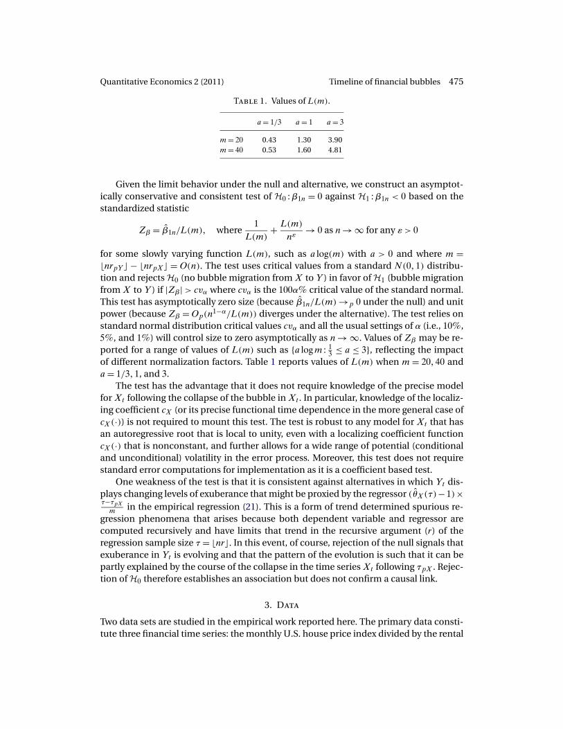
Table 1. Values of L(m).
a= 1/3 a= 1 a= 3
m= 20 0.43 1.30 3.90m= 40 0.53 1.60 4.81
Given the limit behavior under the null and alternative, we construct an asymptot-ically conservative and consistent test of H0 :β1n = 0 against H1 :β1n < 0 based on thestandardized statistic
Zβ = β̂1n/L(m)� where1
L(m)+ L(m)
nε→ 0 as n → ∞ for any ε > 0
for some slowly varying function L(m), such as a log(m) with a > 0 and where m =nrpY � − nrpX� = O(n). The test uses critical values from a standard N(0�1) distribu-tion and rejects H0 (no bubble migration from X to Y ) in favor of H1 (bubble migrationfrom X to Y ) if |Zβ| > cvα where cvα is the 100α% critical value of the standard normal.This test has asymptotically zero size (because β̂1n/L(m) →p 0 under the null) and unitpower (because Zβ = Op(n
1−α/L(m)) diverges under the alternative). The test relies onstandard normal distribution critical values cvα and all the usual settings of α (i.e., 10%,5%, and 1%) will control size to zero asymptotically as n → ∞. Values of Zβ may be re-ported for a range of values of L(m) such as {a logm : 1
3 ≤ a ≤ 3}, reflecting the impactof different normalization factors. Table 1 reports values of L(m) when m = 20�40 anda = 1/3�1, and 3.
The test has the advantage that it does not require knowledge of the precise modelfor Xt following the collapse of the bubble in Xt . In particular, knowledge of the localiz-ing coefficient cX (or its precise functional time dependence in the more general case ofcX(·)) is not required to mount this test. The test is robust to any model for Xt that hasan autoregressive root that is local to unity, even with a localizing coefficient functioncX(·) that is nonconstant, and further allows for a wide range of potential (conditionaland unconditional) volatility in the error process. Moreover, this test does not requirestandard error computations for implementation as it is a coefficient based test.
One weakness of the test is that it is consistent against alternatives in which Yt dis-plays changing levels of exuberance that might be proxied by the regressor (θ̂X(τ)−1)×τ−τpX
m in the empirical regression (21). This is a form of trend determined spurious re-gression phenomena that arises because both dependent variable and regressor arecomputed recursively and have limits that trend in the recursive argument (r) of theregression sample size τ = nr�. In this event, of course, rejection of the null signals thatexuberance in Yt is evolving and that the pattern of the evolution is such that it can bepartly explained by the course of the collapse in the time series Xt following τpX . Rejec-tion of H0 therefore establishes an association but does not confirm a causal link.
3. Data
Two data sets are studied in the empirical work reported here. The primary data consti-tute three financial time series: the monthly U.S. house price index divided by the rental

476 Phillips and Yu Quantitative Economics 2 (2011)
measure from January 1990 to January 2009; monthly crude oil prices (in U.S. dollars)normalized by the oil supply that is approximated by the U.S. inventory from January1999 to January 2009; and the daily spread between the Baa and Aaa bond rates fromJanuary 3, 2006 to July 2, 2009.
A secondary data set is studied to check whether the empirical bubble characteris-tics found in the primary series apply to other commodities. The secondary data includesome commodity prices such as monthly heating oil, coffee, cotton, cocoa, sugar, andfeeder cattle prices, all measured in U.S. dollars, from January 1999 to January 2009.
The choice of the sampling periods is guided by CFG (2008a) because we aim tomatch the empirical analysis with predictions they made. The CFG story begins with theInternet bubble in the Nasdaq in the 1990s (see p. 7 in CFG (2008a)) and ends with thecollapse of all financial bubbles when the economy goes seriously into recession. For theBaa bond rates, it is well known that a relevant event that signaled the effects of the creditcrunch is the failure of Lehman Brothers on September 15, 2008. The sampling periodis chosen so that we have enough observations before September 15 for the bubble testto have good power. Similar arguments apply to the choice of the sampling period forthe exchange rates. Longer sampling intervals, all covering the subprime crisis period,have been used and the empirical findings reported here are robust to the choice ofthe sample period. This is because earlier observations are discarded by the proposedprocedure of selecting the initial observation.
The house price index is the S&P Case–Shiller Composite-10 index obtained fromShiller’s website. We measure fundamental values by standardizing the use of rentaldata. The quarterly rental data are imputed using the method of Davis, Lehnert, andMartin (2008) and are linearly interpolated to a monthly frequency.5 The ratio betweenthe two series is the first time series we use. The crude oil price series is based on WTI–Cushing, Oklahoma spot prices obtained from the Energy Information Administrationwebsite. We measure fundamental values using a measure of the oil supply based onthe inventory of crude oil in the United States.6 The ratio between the two series is thesecond time series we use. The Baa (Aaa) bond rates are averages of Baa (Aaa) industrialbond rates and are obtained from the Federal Reserve Board. The Baa bond rates mea-sure the credit risk level and are particularly relevant because, as the crisis unfolded,the drop in the prices and market liquidity of all mortgage-backed securities led a sharpincreases in the price of risk and in spreads. Unsurprisingly, mistrust among financialcounterparties surged and bond rates jumped. While the same argument may apply tothe Aaa bond rate, the effect is believed to be much less serious for this bond grade. Asa result, the spread between the Baa and Aaa bond rates is a measure of the credit risklevel.
For the secondary data set, all the commodity prices are downloaded from EconStatsat http://www.econstats.com/index.htm and deflated using the Consumer Price Index
5The rental data can be downloaded from http://www.lincolninst.edu/subcenters/land-values/rent-price-ratio.asp.
6The inventory data can be downloaded from the Department of Energy, Monthly Energy Review, U.S.crude oil ending stocks non-SPR (thousands of barrels).

Quantitative Economics 2 (2011) Timeline of financial bubbles 477
Table 2. Summary statistics.
Sample Date DateData Size Freq Min (min) Max (max) DF t
1
House 229 M 0�5405 Sep 1996 1�1418 Feb 2006 −0�3024Oil 121 M 12�086 Feb 1999 146�188 June 2008 −1�5152Baa/Aaa 878 D 0�75 May/2/06 3�50 Dec/3/08 −0�6694
(CPI) obtained from the Department of Labor. Figure 1 plots the three series in the pri-mary data set. Table 2 reports some summary descriptive statistics for these three timeseries, including sample size, sample frequency, sample minimum, date of the mini-mum, sample maximum, date of the maximum, as well as the DF t statistic (DF t
1) basedon the entire sample.
The rental-adjusted house price index troughed in September 1996 and peakedin February 2006. The supply-adjusted crude oil price has its minimum and wandersaround in the early part of the sample, reaching its maximum in mid-2008. The spreadbetween Baa and Aaa moves within a narrow range (between 0.75 and 1.0) in the firsthalf of the sample and reaches its highest point (3.5) on December 3, 2008, shortly afterthe failure of Lehman Brothers on September 15. At the 5% level, in all cases the unitroot null cannot be rejected in favor of an explosive alternative for the full sample (the5% asymptotic critical value is −0.08 for the unit root test statistic DF t
1). That is, the fullsample analysis indicates that no bubble can be found in any of the three time series.
4. Empirical findings
Three phases have been identified in connection with the subprime crisis. Accordingto CFG (2008a), each phase involves a specific hypothesis that concerns related bubbleactivity. In the first phase (A), before the subprime crisis publicly erupted, bubbles hademerged and burst in the stock market, the housing market, and the mortgage market.These bubbles all played a role in global imbalances. The following hypothesis is central.
Hypothesis A. A price bubble arises in the housing market. The property price bubbleoriginated before the subprime crisis surfaced in August 2007 and collapsed as the sub-prime crisis broke.
During the second phase (B), the subprime crisis erupted and funds flowed selec-tively to assets in other markets with lower perceived risk or greater opportunity. In con-sequence, bubbles emerged in certain commodity markets and credit risk perceptionsrapidly elevated, leading to the following hypothesis:
Hypothesis B. Following the public eruption of the subprime crisis, new bubblesemerged in (i) selected commodity price markets and (ii) bond markets.
In the third phase (C), perceptions increased that the financial crisis and associatedcredit crunch might seriously impact real economic activity both in the United States
478 Phillips and Yu Quantitative Economics 2 (2011)
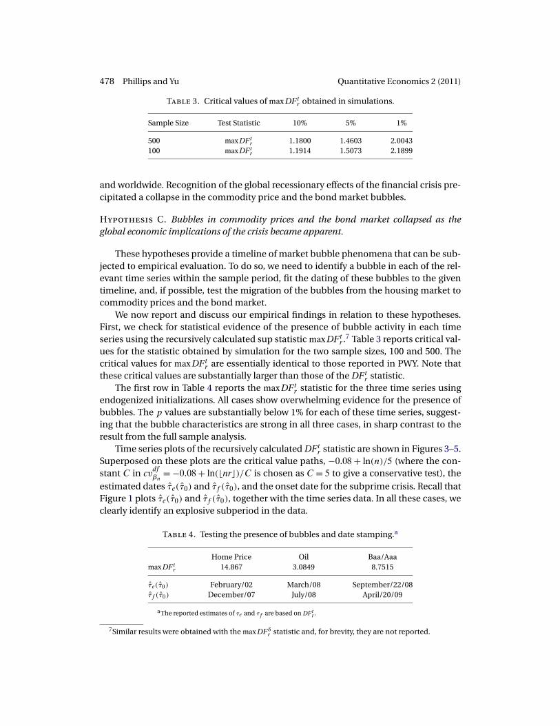
Table 3. Critical values of max DF tr obtained in simulations.
Sample Size Test Statistic 10% 5% 1%
500 max DF tr 1.1800 1.4603 2.0043
100 max DF tr 1.1914 1.5073 2.1899
and worldwide. Recognition of the global recessionary effects of the financial crisis pre-cipitated a collapse in the commodity price and the bond market bubbles.
Hypothesis C. Bubbles in commodity prices and the bond market collapsed as theglobal economic implications of the crisis became apparent.
These hypotheses provide a timeline of market bubble phenomena that can be sub-jected to empirical evaluation. To do so, we need to identify a bubble in each of the rel-evant time series within the sample period, fit the dating of these bubbles to the giventimeline, and, if possible, test the migration of the bubbles from the housing market tocommodity prices and the bond market.
We now report and discuss our empirical findings in relation to these hypotheses.First, we check for statistical evidence of the presence of bubble activity in each timeseries using the recursively calculated sup statistic max DF t
r .7 Table 3 reports critical val-ues for the statistic obtained by simulation for the two sample sizes, 100 and 500. Thecritical values for max DF t
r are essentially identical to those reported in PWY. Note thatthese critical values are substantially larger than those of the DF t
r statistic.The first row in Table 4 reports the max DF t
r statistic for the three time series usingendogenized initializations. All cases show overwhelming evidence for the presence ofbubbles. The p values are substantially below 1% for each of these time series, suggest-ing that the bubble characteristics are strong in all three cases, in sharp contrast to theresult from the full sample analysis.
Time series plots of the recursively calculated DF tr statistic are shown in Figures 3–5.
Superposed on these plots are the critical value paths, −0�08 + ln(n)/5 (where the con-stant C in cv
dfβn
= −0�08 + ln(nr�)/C is chosen as C = 5 to give a conservative test), theestimated dates τ̂e(τ̂0) and τ̂f (τ̂0), and the onset date for the subprime crisis. Recall thatFigure 1 plots τ̂e(τ̂0) and τ̂f (τ̂0), together with the time series data. In all these cases, weclearly identify an explosive subperiod in the data.
Table 4. Testing the presence of bubbles and date stamping.a
Home Price Oil Baa/Aaamax DF t
r 14.867 3.0849 8.7515
τ̂e(τ̂0) February/02 March/08 September/22/08τ̂f (τ̂0) December/07 July/08 April/20/09
aThe reported estimates of τe and τf are based on DF tt .
7Similar results were obtained with the max DFδr statistic and, for brevity, they are not reported.
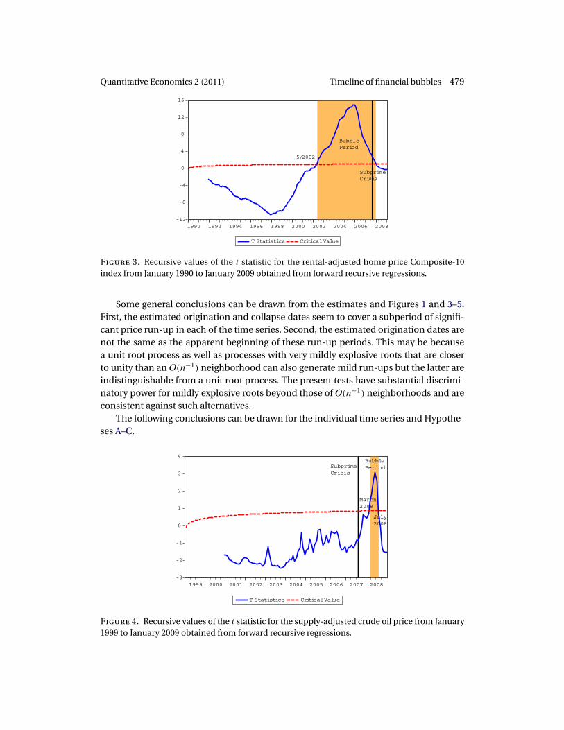
Quantitative Economics 2 (2011) Timeline of financial bubbles 479
Figure 3. Recursive values of the t statistic for the rental-adjusted home price Composite-10index from January 1990 to January 2009 obtained from forward recursive regressions.
Some general conclusions can be drawn from the estimates and Figures 1 and 3–5.First, the estimated origination and collapse dates seem to cover a subperiod of signifi-cant price run-up in each of the time series. Second, the estimated origination dates arenot the same as the apparent beginning of these run-up periods. This may be becausea unit root process as well as processes with very mildly explosive roots that are closerto unity than an O(n−1) neighborhood can also generate mild run-ups but the latter areindistinguishable from a unit root process. The present tests have substantial discrimi-natory power for mildly explosive roots beyond those of O(n−1) neighborhoods and areconsistent against such alternatives.
The following conclusions can be drawn for the individual time series and Hypothe-ses A–C.
Figure 4. Recursive values of the t statistic for the supply-adjusted crude oil price from January1999 to January 2009 obtained from forward recursive regressions.

480 Phillips and Yu Quantitative Economics 2 (2011)
Figure 5. Recursive calculation of the t statistic for the spread between Baa and Aaa bond ratesfrom January 3, 2006 to July 2, 2009, obtained from forward recursive regressions.
• For the rental-adjusted house price series, a significant bubble is found by the DF tr
statistic during the early part of 2000. Our estimate of the bubble origination datein May 2002 strongly supports the argument by Baker (2002), who claimed thatthere was a housing bubble at that time. In addition, according to DF t
r , the bub-ble collapsed in December 2007, soon after the subprime crisis erupted, which isconsistent with Hypothesis A.
• For the supply-adjusted crude oil price, DF tr does not identify a bubble before the
subprime crisis broke. However, a significant bubble is found by DF tr from March
to July 2008. In the left panel of Figure 6, we plot (θ̂X(τ)− 1)τ−τpXm , where θ̂X(τ) is
obtained from the property market, and θ̂Y (τ) − 1, where θ̂Y (τ) is obtained fromthe crude oil market. To test bubble migration from house prices to oil prices, we
(a) Migration from Housing to Oil (b) Migration from Housing to Bonds
Figure 6. Bubble migration between markets. Panel (a) plots (θ̂X(τ)− 1) τ−τpXm for the housing
market and (θ̂Y (τ) − 1) from the oil market between November 2005 and June 2008. Panel (b)plots (θ̂X(τ)−1) τ−τpX
m for the house market and (θ̂Y (τ)−1) from the bond market between May2006 and October 2008.

Quantitative Economics 2 (2011) Timeline of financial bubbles 481
Table 5. Values of Zβ to test migration from thehousing market to the oil market.
a= 1/3 a= 1 a= 3
m= 32 −20.85 −6.95 −2.33
ran the empirical regression (19) with rp being selected by the t statistic. The pointestimate of β1 is −10.46. Table 5 shows the values of Zβ for L(m) = a log(m) witha= 1/3�1, and 3. These values are all significant at the 1% level. The results suggestvery strong evidence of bubble migration from the housing market to the oil pricemarket, consistent with Hypothesis B(i).
• For the time series spread between the Baa and Aaa bond rates, the DF tr statistic
suggests random wandering behavior in the series for much of the period but re-veals a significant bubble from September 22, 2008 to April 20, 2009. This periodcorresponds to the rapid acceleration of financial distress in the weeks followingthe Lehman Brothers bankruptcy on September 15, 2008. To test bubble migrationfrom house prices to bond prices, we ran the empirical regression (19) with rp be-ing selected by the t statistic. In the right panel of Figure 6, we plot (θ̂X(τ) − 1) τn ,where θ̂X(τ) relates to the house market, and θ̂Y (τ)− 1, where θ̂Y (τ) relates to thebond market. The point estimate of β1 is −12.00. Table 6 shows the values of Zβ
for L(m) = a log(m) with a = 1/3�1, and 3. These values are all significant at the1% level. The results suggest very strong evidence of bubble migration from thehousing market to the bond market, consistent with Hypothesis B(ii).
• The bubble in the oil price market collapsed in July 2008 and the bubble in thebond market collapsed on April 20, 2009. Both findings are consistent with Hy-pothesis C.
In sum, the tests reveal bubble characteristics in the data that are consistent withHypotheses A–C. The empirical estimates of the crisis timeline broadly support the pre-dictions made in the CFG (2008a) model. Figure 7 shows the complete timeline of thebubble phenomena in a profile using the recursive tests. The timeline shows how bub-bles migrated from the property market following the subprime crisis to certain goodsin the commodity markets and then to the bond market.
To assess whether these bubble characteristics were generic or specific features ofcommodity and financial markets during the subprime crisis and its aftermath, we ap-plied the methods more broadly to many series in a secondary data set. To preserve
Table 6. Values of Zβ to test migration from thehousing market to the bond market.
a= 1/3 a= 1 a= 3
m= 30 −24.37 −8.12 −2.71

482 Phillips and Yu Quantitative Economics 2 (2011)
Figure 7. Timeline of financial bubbles in the real estate, commodity, and bond markets. Thepanels show recursive calculations of the DF t statistic and critical values highlighting the suc-cessive bubble episodes.
space, we present only summary empirical results of these findings in Table 7 withoutplotting the recursive test statistics.
Although it is clear from the empirical results obtained earlier that funds movedacross markets during the crisis period for flight-to-quality and flight-to-liquidity rea-sons, the results in Table 7 suggest that investors were selective in transferring assets.For example, in the commodity market, we identify a bubble in heating oil prices, withsimilar origination and collapsing dates as those for crude oil prices. However, we findno evidence of bubbles in coffee, cotton, sugar, and feeder cattle prices.
5. Conclusions
This paper provides an empirical study of the bubble characteristics in several key fi-nancial variables over an historical time period that includes the subprime crisis and its
Table 7. Test results for the presence of bubbles and date stamps.
max DF tr τ̂e τ̂f
Heating oil 2�2416 March/08 August/08Coffee −0�7002 NA NACotton −0�0866 NA NACocoa 0�9872 NA NASugar −0�2220 NA NAFeeder cattle 0�4327 NA NA
Quantitative Economics 2 (2011) Timeline of financial bubbles 483
sequel, including global effects. The econometric methods employed are based on re-cursive regression, right-sided unit root tests, and a newly developed dating technologyand associated limit theory from Phillips and Yu (2009) and Phillips, Shi, and Yu (2011).The methods are complemented by a mechanism for testing potential migration acrossmarkets. The dating techniques enable us to track the timeline of the crisis in terms ofthe individual series by empirically determining the origination and collapse of eachof the bubbles. The dates are matched against the onset date for the subprime crisis aswell as a specific sequential hypothesis concerning bubble migrations that are predictedin the theoretical model proposed by CFG (2008a). Our estimates suggest that bubblesemerged in the housing market before the subprime crisis and collapsed with the sub-prime crisis. The bubble then migrated from the housing market to selected commoditymarkets and the bond market after the crisis erupted into the public arena. All thesebubbles collapsed as the financial crisis impacted real economic activity. The estimatedsequence of the bubble migration phenomenon is broadly consistent with the predic-tions of CFG (2008a).
The methods used here can be used to provide early warning diagnostics for marketexuberance as they provide consistent tests for mildly explosive behavior. Such diag-nostics may assist policy makers in framing early monetary policy responses or otherregulatory actions or interventions to combat speculative bubbles in financial markets.
Appendix: Limit theory for the bubble migration test
Consistent with the notion of bubble migration and to fix ideas, it is subsequently as-sumed that the period of bubble collapse in Xt is relatively short prior to the emer-gence of exuberance in Yt . We therefore set τpX = τeY + o(n). Then τpX = nrpX� =nreY �{1 + o(1)} and we define m = nrpY � − nrpX�.
The empirical regression version of (19) has the form
θ̂Y (τ)− 1 = β̂0n + β̂1n(θ̂X(τ)− 1)τ − τpX
m+ error (21)
over the interval τ ∈ (τpX�τpY ]. Our first interest is in the null behavior of the fitted slopecoefficient
β̂1n =
nrpY �∑τ=nrpX�
Z̃Y (τ)Z̃X(τ)
nrpY �∑τ=nrpX�
Z̃X(τ)2
�
where
ZY(τ) = θ̂Y (τ)− 1� ZX(τ) = (θ̂X(τ)− 1)τ − τpX
m
484 Phillips and Yu Quantitative Economics 2 (2011)
and
Z̃a(τ) =Za(τ)−m−1nrpY �∑
s=nrpX�Za(s) for a=X�Y�
Under the null hypothesis θY (τ) = 1 + cYnα , the estimation error θ̂Y (τ) − θY (τ) has the
asymptotic behavior (as shown in Phillips, Shi, and Yu (2011))
nαθτ−τeYn
2cY(θ̂Y (τ)− θY (τ)) ⇒
1r
∫ reY
0BY(s)ds
BY (re)=: 1
rC say. (22)
Here C = ∫ reY0 BY(s)ds/BY (re) is a Cauchy-like random variable, being a ratio of corre-
lated normal variables, and BY(s) is the Brownian motion (or more general Gaussianprocess) corresponding to the limit under weak convergence of the standardized seriesn−1/2Yns� prior to exuberance in Yt (i.e., for s < reY ). Then
nZY (nr�) = n(θ̂Y (τ)− 1) = n(θY (τ)− 1)+ n(θ̂Y (τ)− θY (τ))(23)
= n1−αcY + n1−α2cYrθ
τ−τeYY
C{1 + op(1)} for r > reY �
It follows that
nZ̃Y (τ) = nZY (τ)− n
nrpY �∑k=nrpX�
ZY(k)
nrpY � − nrpX�
= n1−α2cYC
⎧⎪⎪⎪⎪⎪⎪⎨⎪⎪⎪⎪⎪⎪⎩
1
rθτ−τeYY
−
τpY∑k=τeY
1
θk−τeYY (k/n)
nrpY � − nrpX�
⎫⎪⎪⎪⎪⎪⎪⎬⎪⎪⎪⎪⎪⎪⎭
{1 + op(1)}
= n1−α2cYC
{1
rθτ−τeYY
− 1(rpY − reY )
∫ rpY
reY
e−cY (s−reY )n1−α
s
}(24)
× {1 + op(1)}
∼ n1−α2cYC
{1
rθτ−τeYY
− 1n1−α(rpY − reY )reY cY
}�
since as n → ∞,
1n
τpY∑k=τeY
1
θk−τeYY (k/n)
=∫ rpY
reY
e−cY (s−reY )n1−α
sds{1 + o(1)}
Quantitative Economics 2 (2011) Timeline of financial bubbles 485
=∫ rpY−reY
0
e−cYpn1−α
p+ reYdp{1 + o(1)}
(25)
= 1n1−α
∫ (rpY−reY )n1−α
0
e−cY q
reY + q/n1−αdq{1 + o(1)}
= 1n1−αreY cY
{1 + o(1)}�
A more general version of this type of asymptotic approximation is developed in (28)below.
To obtain the corresponding limit theory for θ̂X(τ), we assume that from the bubblepeak τ = nrpX�, the autoregressive coefficient θX(τ) falls rapidly during the collapseperiod to the immediate vicinity of unity. We use data from [τpX�τpY ] to compute θ̂X(τ)
recursively for τ = nr� by least squares regression, giving data for the regressor in (21),namely
nZX(nr�) = n(θ̂X(τ)− 1)τ − τpX
m
= n(θ̂X(τ)− θX(τ))τ − τpX
m+ n(θX(τ)− 1)
τ − τpX
m(26)
∼
r − rpX
rpY − rpX
∫ r
rpX
W̃X(s)dWX(s)
∫ r
rpX
W̃ 2X(s)
+ r − rpX
rpY − rpXcX
=: r − rpX
rpY − rpXhX(r)+ r − rpX
rpY − rpXcX =: gX(r)�
where W̃X(s) = WX(s) − 1r
∫ r0 WX(p)dp for s ∈ [0� r] is a Gaussian process (a demeaned
Brownian motion if θX(τ) = 1 and a demeaned diffusion if θX = 1 + cX/n for some con-stant localizing coefficient cX ). Since the regressor in (21) is ZX(τ) = (θ̂X(τ) − 1)τ−τpX
m ,we define the demeaned and scaled variable for τ = nr� over the sample period(τpX�τpY ] as
nZ̃X(τ) = nZX(τ)− n
nrpY �∑k=nrpX�
ZX(k)
nrpY � − nrpX�
∼ gX(r)− 1rpY − rpX
∫ rpY
rpX
gX(s)ds =: g̃X(r)�
An important aspect of the migration test is that it does not require explicit characteriza-tion of the limit process W̃X(s) or the demeaned process g̃X(r), thereby accommodatingany value of θX that is local to unity and various forms of unconditional and conditionalheterogeneity in the Xt error process. The null hypothesis is therefore highly compositein terms of potential generating mechanisms leading to the limit process W̃X .
486 Phillips and Yu Quantitative Economics 2 (2011)
Under the null, we have
β̂1n =
nrpY �∑τ=nrpX�
Z̃Y (τ)Z̃X(τ)
nrpY �∑τ=nrpX�
Z̃X(τ)2
=
1n
nrpY �∑τ=nrpX�
{nZ̃Y (τ)}{nZ̃X(τ)}
1n
nrpY �∑τ=nrpX�
{nZ̃X(τ)}2
∼n1−α2cYC
1n
nrpY �∑τ=nrpX�
{nZ̃X(τ)}{
1
θτ−τeY τ/n
− 1n1−α(rpY − reY )reY cY
}∫ rpY
rpX
g̃X(s)2 ds
=n1−α2cYC
∫ rpY
reY
g̃X(s)s−1e−cY n1−α(s−reY ) ds∫ rpY
rpX
g̃X(s)2 ds
(27)
∼ n1−α2cYC∫ rpY
rpX
g̃X(s)2 ds
g̃X(reY )
n1−αcY reY
∼ 2Cg̃X(reY )
reY
∫ rpY
rpX
g̃X(s)2 ds
�
Here we use the fact that
1/θτ−τeY = 1
/(1 + cY
nα
)τ−τe
∼ e−cY n1−α(r−reY )
and employ the asymptotic approximation
∫ b
af (s)e−cnγ(s−a) ds =
∫ b−a
0f (p+ a)e−cnγp dp
=∫ (b−a)nγ
0f
(a+ q
nγ
)e−cq dq/nγ (28)
∼ f (a)
nγ
∫ ∞
0e−cq dq = f (a)
nγc�
to the integral in the numerator of (27), of which (25) above is a special case and forwhich there are other uses. It follows that
β̂1n ⇒ 2Cg̃X(reY )
reY∫ rpYrpX
g̃X(s)2 ds� (29)
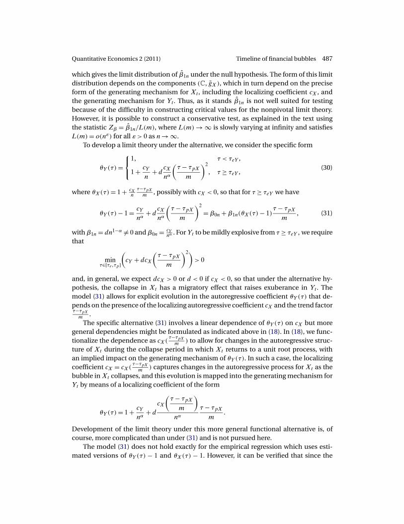
Quantitative Economics 2 (2011) Timeline of financial bubbles 487
which gives the limit distribution of β̂1n under the null hypothesis. The form of this limitdistribution depends on the components (C� g̃X), which in turn depend on the preciseform of the generating mechanism for Xt , including the localizing coefficient cX , andthe generating mechanism for Yt . Thus, as it stands β̂1n is not well suited for testingbecause of the difficulty in constructing critical values for the nonpivotal limit theory.However, it is possible to construct a conservative test, as explained in the text usingthe statistic Zβ = β̂1n/L(m), where L(m) → ∞ is slowly varying at infinity and satisfiesL(m) = o(nε) for all ε > 0 as n→ ∞.
To develop a limit theory under the alternative, we consider the specific form
θY (τ) =⎧⎨⎩
1� τ < τeY ,
1 + cYn
+ dcXnα
(τ − τpX
m
)2
� τ ≥ τeY ,(30)
where θX(τ) = 1 + cXn
τ−τpXm , possibly with cX < 0, so that for τ ≥ τeY we have
θY (τ)− 1 = cYnα
+ dcXnα
(τ − τpX
m
)2
= β0n +β1n(θX(τ)− 1)τ − τpX
m� (31)
with β1n = dn1−α �= 0 and β0n = cYnα . For Yt to be mildly explosive from τ ≥ τeY � we require
that
minτ∈[τe�τp]
(cY + dcX
(τ − τpX
m
)2)> 0
and, in general, we expect dcX > 0 or d < 0 if cX < 0, so that under the alternative hy-pothesis, the collapse in Xt has a migratory effect that raises exuberance in Yt . Themodel (31) allows for explicit evolution in the autoregressive coefficient θY (τ) that de-pends on the presence of the localizing autoregressive coefficient cX and the trend factorτ−τpX
m .The specific alternative (31) involves a linear dependence of θY (τ) on cX but more
general dependencies might be formulated as indicated above in (18). In (18), we func-tionalize the dependence as cX(
τ−τpXm ) to allow for changes in the autoregressive struc-
ture of Xt during the collapse period in which Xt returns to a unit root process, withan implied impact on the generating mechanism of θY (τ). In such a case, the localizingcoefficient cX = cX(
τ−τpXm ) captures changes in the autoregressive process for Xt as the
bubble in Xt collapses, and this evolution is mapped into the generating mechanism forYt by means of a localizing coefficient of the form
θY (τ) = 1 + cYnα
+ d
cX
(τ − τpX
m
)nα
τ − τpX
m�
Development of the limit theory under this more general functional alternative is, ofcourse, more complicated than under (31) and is not pursued here.
The model (31) does not hold exactly for the empirical regression which uses esti-mated versions of θY (τ) − 1 and θX(τ) − 1. However, it can be verified that since the

488 Phillips and Yu Quantitative Economics 2 (2011)
formulation given in (31) still produces a mildly explosive process in Yt , we have the
relationship, (just as in the basic case (22) where β1n = 0 and θY (τ) = 1 + cYnα )
θ̂Y (τ)− 1 = θY (τ)− 1 + (θ̂Y (τ)− θY (τ))
= θY (τ)− 1 +Op
(1
nαθτ−τeYn�min
)�
with
θn�min = 1 +min
τ∈[τe�τp]
{cY + dcX
(τ − τpX
m
)2}nα
�
which involves a negligible estimation error. The estimation error in θ̂X(τ) is, as before,
θ̂X(τ)− 1 = (θX(τ)− 1)+ (θ̂X(τ)− θX(τ)) ∼ (θX(τ)− 1)+ 1nhX
(τ
n
)�
since from (26) we have n(θ̂X(τ)− θX(τ)) ⇒ hX(r) for τ = nr�. So the fitted model can
be written in the form
θ̂Y (τ)− 1 = cYnα
+ dn(θX(τ)− 1)
nατ − τpX
m+Op
(1
nαθτ−τeYn�min
)
= cYnα
+ dn(θ̂X(τ)− 1)
nατ − τpX
m+ d
(θX(τ)− θ̂X(τ))n
nατ − τpX
m
+Op
(1
nαθτ−τeYn�min
)
∼ cYnα
+ dn(θ̂X(τ)− 1)
nατ − τpX
m− d
nαhX
(τ
n
)τ − τpX
m
= β0n +β1n
{(θ̂X(τ)− 1)
τ − τpX
m− 1
nhX
(τ
n
)τ − τpX
m
}�
If d = 0, then β1n = 0 and null behavior is the same as that described above. If d �= 0, then
the limit behavior under the alternative is
β̂1n =
nrpY �∑τ=nrpX�
Z̃Y (τ)Z̃X(τ)
nrpY �∑τ=nrpX�
Z̃X(τ)2

Quantitative Economics 2 (2011) Timeline of financial bubbles 489
= β1n
⎧⎪⎪⎪⎪⎪⎪⎨⎪⎪⎪⎪⎪⎪⎩
nrpY �∑τ=nrpX�
Z̃X(τ)2
nrpY �∑τ=nrpX�
Z̃X(τ)2
−
1n
nrpY �∑τ=nrpX�
Z̃X(τ)hX
(τ
n
)τ − τpX
m
nrpY �∑τ=nrpX�
Z̃X(τ)2
⎫⎪⎪⎪⎪⎪⎪⎬⎪⎪⎪⎪⎪⎪⎭
= β1n
⎧⎪⎪⎪⎪⎪⎪⎨⎪⎪⎪⎪⎪⎪⎩
1 −
1n
nrpY �∑τ=nrpX�
(nZ̃X(τ))hX
(τ
n
)τ − τpX
m
1n
nrpY �∑τ=nrpX�
(nZ̃X(τ))2
⎫⎪⎪⎪⎪⎪⎪⎬⎪⎪⎪⎪⎪⎪⎭
∼ dn1−α
⎧⎪⎪⎪⎨⎪⎪⎪⎩
∫ rpY
rpX
g̃X(s)
(g̃x(s)− hX(s)
s − rpX
rpY − rpX
)ds
∫ rpY
rpX
g̃X(s)2 ds
⎫⎪⎪⎪⎬⎪⎪⎪⎭�
From (26), we have hX(s)s−rpX
rpY−rpX+ cX
s−rpXrpY−rpX
= gX(s). Then
∫ rpY
rpX
g̃X(s)
(g̃X(s)− hX(s)
s − rpX
rpY − rpX
)ds = cX
∫ rpY
rpX
g̃X(s)s − rpX
rpY − rpXds �= 0�
provided that∫ reYrpX
g̃X(s)s−rpX
rpY−rpXds �= 0 and cX �= 0. It follows that the statistic β̂1n =
Op(n1−α) and is divergent under the alternative hypothesis H1 :β1n �= 0. We deduce that
the test statistic Zβ = β̂1n/L(m) leads to an asymptotically conservative test under thenull when a fixed critical value from the standard normal distribution is used becauseZβ →p 0 and the test is consistent under the alternative H1 : β1n �= 0, provided thatcX �= 0.
Figures 8 and 9 show densities of Zβ = β̂1n/ ln(m) under H0 and H1 for varioussample sizes for a model with localizing coefficients cX = −2 (for the period of col-lapse for the Xt series), cY = 1, α = 0�85, and d = −3 for the mildly explosive au-
Figure 8. Densities of Zβ under the null.
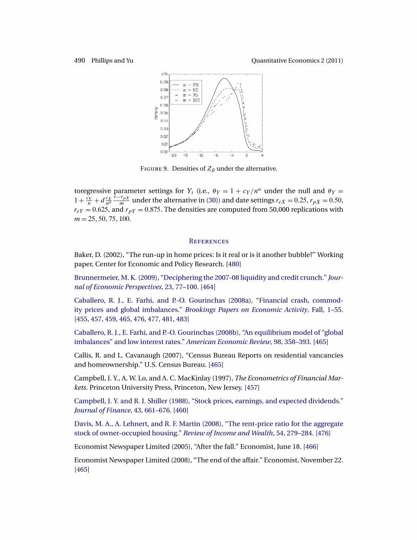
490 Phillips and Yu Quantitative Economics 2 (2011)
Figure 9. Densities of Zβ under the alternative.
toregressive parameter settings for Yt (i.e., θY = 1 + cY /nα under the null and θY =
1 + cYn + d cX
nατ−τpX
m under the alternative in (30)) and date settings reX = 0�25, rpX = 0�50,reY = 0�625, and rpY = 0�875. The densities are computed from 50,000 replications withm= 25�50�75�100.
References
Baker, D. (2002), “The run-up in home prices: Is it real or is it another bubble?” Workingpaper, Center for Economic and Policy Research. [480]
Brunnermeier, M. K. (2009), “Deciphering the 2007-08 liquidity and credit crunch.” Jour-nal of Economic Perspectives, 23, 77–100. [464]
Caballero, R. J., E. Farhi, and P.-O. Gourinchas (2008a), “Financial crash, commod-ity prices and global imbalances.” Brookings Papers on Economic Activity, Fall, 1–55.[455, 457, 459, 465, 476, 477, 481, 483]
Caballero, R. J., E. Farhi, and P.-O. Gourinchas (2008b), “An equilibrium model of “globalimbalances” and low interest rates.” American Economic Review, 98, 358–393. [465]
Callis, R. and L. Cavanaugh (2007), “Census Bureau Reports on residential vancanciesand homeownership.” U.S. Census Bureau. [465]
Campbell, J. Y., A. W. Lo, and A. C. MacKinlay (1997), The Econometrics of Financial Mar-kets. Princeton University Press, Princeton, New Jersey. [457]
Campbell, J. Y. and R. J. Shiller (1988), “Stock prices, earnings, and expected dividends.”Journal of Finance, 43, 661–676. [460]
Davis, M. A., A. Lehnert, and R. F. Martin (2008), “The rent-price ratio for the aggregatestock of owner-occupied housing.” Review of Income and Wealth, 54, 279–284. [476]
Economist Newspaper Limited (2005), “After the fall.” Economist, June 18. [466]
Economist Newspaper Limited (2008), “The end of the affair.” Economist, November 22.[465]
Quantitative Economics 2 (2011) Timeline of financial bubbles 491
Evans, G. W. (1991), “Pitfalls in testing for explosive bubbles in asset prices.” AmericanEconomic Review, 81, 922–930. [457, 468]
Greenlaw, D., J. Hatzius, A. Kashyap, and H. S. Shin (2008), “Leveraged losses: Lessonsfrom the mortgage market meltdown.” U.S. Monetary Policy Forum Report 2. [464]
Hull, J. (2008), “The credit crunch of 2007: What went wrong? Why? What lessons can belearned?” Working paper, Rotman School of Management, University of Toronto. [464]
Lee, J.-H. and P. C. B. Phillips (2011), “Asset pricing with financial bubble risk.” Workingpaper, Yale University. [460]
Phillips, P. C. B. (1987), “Time series regression with a unit root.” Econometrica, 55,277–301. [467]
Phillips, P. C. B. (1996), “Econometric model determination.” Econometrica, 64, 763–812.[471]
Phillips, P. C. B. (2008), “Unit root model selection.” Journal of the Japan Statistical Soci-ety, 38, 65–74. [472]
Phillips, P. C. B. and T. Magdalinos (2007a), “Limit theory for moderate deviations froma unit root.” Journal of Econometrics, 136, 115–130. [457, 466, 467, 469]
Phillips, P. C. B. and T. Magdalinos (2007b), “Limit theory for moderate deviations fromunity under weak dependence.” In The Refinement of Econometric Estimation and TestProcedures: Finite Sample and Asymptotic Analysis (G. D. A. Phillips and E. Tzavalis, eds.)123–162. Cambridge University Press, Cambridge. [457, 466, 469]
Phillips, P. C. B. and T. Magdalinos (2009), “Unit root and cointegrating limit theory wheninitialization is in the infinite past.” Econometric Theory, 25, 1682–1715. [471]
Phillips, P. C. B., S. Shi, and J. Yu (2011), “Testing for multiple bubbles.” Working paper,Yale University. [458, 466, 471, 474, 483, 484]
Phillips, P. C. B., Y. Wu, and J. Yu (2011), “Explosive behavior in the 1990s Nasdaq: Whendid exuberance escalate asset values?” International Economic Review, 52, 201–226.[455, 457, 466, 468]
Phillips, P. C. B. and J. Yu (2009), “Limit theory for dating the origination and collapse ofmildly explosive periods in time series data.” Unpublished manuscrip, Sim Kee Boon In-stitute for Financial Economics, Singapore Management University. [458, 466, 468, 469,483]
Schwarz, G. (1978), “Estimating the dimension of a model.” Annals of Statistics, 6,461–464. [471]
Submitted May, 2010. Final version accepted July, 2011.