dataflow interchange format and a … interchange format and a framework for processing dataflow...
TRANSCRIPT
DATAFLOW INTERCHANGE FORMAT AND A FRAMEWORK FORPROCESSING DATAFLOW GRAPHS
by
Fuat Keceli
Thesis submitted to the Faculty of the Graduate School of theUniversity of Maryland, College Park in partial fulfillment
of the requirement for the degree ofMaster of Science
2004
Advisory Committee:
Dr. Shuvra S. Bhattacharyya, ChairDr. Ankur SrivastavaDr. Gang Qu

DEDICATION
To my mother, father and brother.
Report Documentation Page Form ApprovedOMB No. 0704-0188
Public reporting burden for the collection of information is estimated to average 1 hour per response, including the time for reviewing instructions, searching existing data sources, gathering andmaintaining the data needed, and completing and reviewing the collection of information. Send comments regarding this burden estimate or any other aspect of this collection of information,including suggestions for reducing this burden, to Washington Headquarters Services, Directorate for Information Operations and Reports, 1215 Jefferson Davis Highway, Suite 1204, ArlingtonVA 22202-4302. Respondents should be aware that notwithstanding any other provision of law, no person shall be subject to a penalty for failing to comply with a collection of information if itdoes not display a currently valid OMB control number.
1. REPORT DATE 2004 2. REPORT TYPE
3. DATES COVERED 00-00-2004 to 00-00-2004
4. TITLE AND SUBTITLE Dataflow Interchange Format and a Framework for Processing DataflowGraphs
5a. CONTRACT NUMBER
5b. GRANT NUMBER
5c. PROGRAM ELEMENT NUMBER
6. AUTHOR(S) 5d. PROJECT NUMBER
5e. TASK NUMBER
5f. WORK UNIT NUMBER
7. PERFORMING ORGANIZATION NAME(S) AND ADDRESS(ES) University of Maryland,Department of Electrical and ComputerEngineering,Institute for Advanced Computer Studies,College Park,MD,20742
8. PERFORMING ORGANIZATIONREPORT NUMBER
9. SPONSORING/MONITORING AGENCY NAME(S) AND ADDRESS(ES) 10. SPONSOR/MONITOR’S ACRONYM(S)
11. SPONSOR/MONITOR’S REPORT NUMBER(S)
12. DISTRIBUTION/AVAILABILITY STATEMENT Approved for public release; distribution unlimited
13. SUPPLEMENTARY NOTES
14. ABSTRACT
15. SUBJECT TERMS
16. SECURITY CLASSIFICATION OF: 17. LIMITATION OF ABSTRACT
18. NUMBEROF PAGES
129
19a. NAME OFRESPONSIBLE PERSON
a. REPORT unclassified
b. ABSTRACT unclassified
c. THIS PAGE unclassified
Standard Form 298 (Rev. 8-98) Prescribed by ANSI Std Z39-18
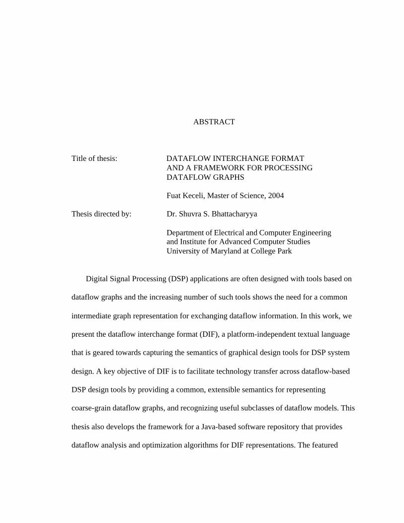
ABSTRACT
Title of thesis: DATAFLOW INTERCHANGE FORMAT AND A FRAMEWORK FOR PROCESSING DATAFLOW GRAPHS
Fuat Keceli, Master of Science, 2004
Thesis directed by: Dr. Shuvra S. Bhattacharyya
Department of Electrical and Computer Engineering and Institute for Advanced Computer Studies University of Maryland at College Park
Digital Signal Processing (DSP) applications are often designed with tools based on
dataflow graphs and the increasing number of such tools shows the need for a common
intermediate graph representation for exchanging dataflow information. In this work, we
present the dataflow interchange format (DIF), a platform-independent textual language
that is geared towards capturing the semantics of graphical design tools for DSP system
design. A key objective of DIF is to facilitate technology transfer across dataflow-based
DSP design tools by providing a common, extensible semantics for representing
coarse-grain dataflow graphs, and recognizing useful subclasses of dataflow models. This
thesis also develops the framework for a Java-based software repository that provides
dataflow analysis and optimization algorithms for DIF representations. The featured

framework is accompanied by toolboxes for hierarchical design support and visualization
of graphs.

ACKNOWLEDGEMENTS
I would like to acknowledge the patient help and guidance given to me by my advisor,
Dr. Shuvra S. Bhattacharyya, throughout the course of developing this thesis. I would also
like to thank Shahrooz Shahparnia, Ming-Yung Ko and the members of the DSP-CAD
group for their assistance, support and friendship.
This research was sponsored in part by the Defense Advanced Research Projects
Agency (Contract number F30602-01-C-0171, through the University of Southern
California Information Sciences Institute).
iv
TABLE OF CONTENTS
List of Figures................................................................................................................... vi
Chapter 1: Introduction................................................................................................1
1.1. DIF Package..........................................................................................21.2. Organization of Thesis ..........................................................................21.3. Notation ................................................................................................3
Chapter 2: Background ................................................................................................4
2.1. Graphs ...................................................................................................42.2. Dataflow Graphs ...................................................................................82.3. Defining Formal Languages .................................................................92.4. The Java Programming Language ......................................................13
Chapter 3: Dataflow Interchange Format ................................................................16
3.1. The Language .....................................................................................183.1.1. Lexical Conventions ............................................................183.1.2. The Body of a DIF Specification .........................................193.1.3. Defining the Topology of a Graph.......................................203.1.4. Hierarchical Graphs .............................................................223.1.5. User-defined and Built-in Attributes ...................................253.1.6. Parameters............................................................................263.1.7. The basedon Feature............................................................273.1.8. Preprocessor Support ...........................................................283.1.9. Scope of a Graph..................................................................283.1.10. Summary of Keywords ......................................................30
3.2. Supported Graph Types ......................................................................303.2.1. DIF Graphs ..........................................................................313.2.2. CSDF Graphs .......................................................................313.2.3. SDF Graphs..........................................................................323.2.4. Single Rate and HSDF Graphs ............................................32
3.3. A Complete DIFGraph Definition Example.......................................33
Chapter 4: DIF Package .............................................................................................36
4.1. Organization of Classes ......................................................................374.2. Generic Graphs ...................................................................................39
4.2.1. Overview of Elementary Classes.........................................404.2.2. Cloning and Mirroring Graphs ............................................43
4.3. The DIFGraph Class and mapss.dif Package......................................44
v
The Attribute Mechanism ..................................................44Parametrization of Attributes .............................................45
4.3.1. DIF Language Conversion from DIFGraph Objects ...........464.3.2. Dataflow Graph Classes.......................................................47
4.4. The Hierarchy Package .......................................................................494.4.1. Overview of Classes ............................................................514.4.2. Hierarchy Related Functions ...............................................544.4.3. Extending the Hierarchy Class ............................................584.4.4. DIF Language Conversion from DIFHierarchy Objects .....58
4.5. The DIF Compiler ...............................................................................584.5.1. SableCC ...............................................................................59
DIF Parser Design with SableCC ......................................60The Language Specification File .......................................60The Compiler .....................................................................64
4.5.2. The Language Analysis Class ..............................................644.5.3. Extending the DIF Language For A New Graph Type ........654.5.4. The Reader Class – The Front-End Compiler .....................66
4.6. The DIF Writer ...................................................................................674.7. Graph Visualization ............................................................................684.8. Summary of DIF API Packages and Classes ......................................69
Chapter 5: Application Examples and Tutorials......................................................71
5.1. Applications ........................................................................................715.1.1. Ptolemy ................................................................................715.1.2. MCCI Autocoding Toolset ..................................................725.1.3. Benchmark Generation ........................................................74
5.2. Tutorials ..............................................................................................765.2.1. A Tutorial Example for the Visualization Tool ...................765.2.2. Tutorial Examples for the Hierarchy Mechanism................79
Hierarchy Example ............................................................80Directed Hierarchy Example .............................................87
5.2.3. A Tutorial Example for the DIF Compiler ..........................91
Chapter 6: Conclusion ................................................................................................95
Appendix A: The Complete DIF Language..................................................................96
Appendix B: SableCC Language Specification Input ...............................................101
Appendix C: Class Designs in the Unified Modeling Language ...............................105
Appendix D: DIF Graph and Hierarchy Specification Examples............................111
vi
LIST OF FIGURES
Figure 2-1. Examples of graph types. ..................................................................................6
Figure 2-2. Illustration of a depth first tree walk. ................................................................7
Figure 2-3. A dataflow graph example and firing of a dataflow graph. ..............................8
Figure 2-4. Parse tree and the AST for the string y=2*3-5+6........................................14
Figure 3-1. A sketch of a dataflow graph definition in DIF. .............................................17
Figure 3-2. An example of a graph and its topology definition specified in DIF..............21
Figure 3-3. Definition of DIF graphs with interfaces and super nodes. ............................24
Figure 3-4. Definition of a high level graph with two subgraphs. .....................................33
Figure 3-5. Definitions for Graphs 2, 3 and 4....................................................................34
Figure 4-1. DIF package design.........................................................................................39
Figure 4-2. An example of defining a basic graph. ...........................................................42
Figure 4-3. Source DIF specification used in Figure4-4. .................................................47
Figure 4-4. A conversion from a DIF specification to Java code with the DIF package API.48
Figure 4-5. A summary of connection schemes for a port.................................................50
Figure 4-6. The Java code that defines and flattens the nested hierarchy 2. .....................53
Figure 4-7. DIF parser design flow....................................................................................61
Figure 4-8. A simple SableCC generated compiler front-end. ..........................................64
vii
Figure 5-1. Ptolemy II model of a pulse amplitude modulation system that is exported to DIF. ..................................................................................................................71
Figure 5-2. The top-level partitioned application graph of a SAR application and a range processing graph in the MCCI Autocoding Toolset. .......................................72
Figure 5-3. Range processing and range processing instantiation in SAR. .......................73
Figure 5-4. A synthetic DIFGraph generated by the DIF package and dot generator output for the graph. ....................................................................................................75
Figure 5-5. Undirected and directed layouts of the same graph with false and true options set in DotGenerator.toFile method................................................................76
Figure 5-6. A customized graph with circular and colored nodes. ....................................77
Figure 5-7. A clustered graph example..............................................................................80
Figure 5-8. Dot output for hierarchy 0. .............................................................................81
Figure 5-9. Dot outputs for hierarchy 1 before and after it is flattened.............................83
Figure 5-10. Dot outputs for hierarchy 2 before and after it is flattened...........................84
Figure 5-11. Dot outputs for hierarchy 3 before and after it is flattened...........................86
Figure 5-12. Dot outputs for hierarchy tree graph. ............................................................87
Figure 5-13. Hierarchy 3 with its first level subgraphs. ....................................................89
Figure 5-14. Hierarchy 3 after the deep-flatten command.................................................90
Figure C-1. UML diagram for the basic classes of mapss.dif........................................106
Figure C-2. UML diagram for the utility classes of mapss.dif. .....................................107
Figure C-3. UML diagram for the classes of mapss.dif.language. ..............................108
viii
Figure C-4. UML diagram for the classes of mapss.graph.hierarchy. ........................109
Figure C-5. UML diagram for the classes of mapss.graph. ..........................................110
Figure D-1. GraphViz outputs for the hierarchies defined in this appendix - all hierarchies are flattened one level. ...................................................................................117
1
CHAPTER 1
Introduction
Modeling of DSP applications based on coarse-grain dataflow graphs is widespread in
the DSP design community, and a large and growing set of DSP design tools support such
dataflow semantics [3]. Since a variety of dataflow modeling styles and accompanying
semantic constructs have been developed for DSP design tools (e.g., see [2,5,6,8,12,13]), a
critical problem in the process of technology transfer to, from, and across such tools is a
common, vendor-independent language and associated suite of intermediate
representations and algorithms for DSP-oriented dataflow modeling.
As motivated above, DIF is not centered around any particular form of dataflow, and
is designed instead to express different kinds of dataflow semantics. The present version of
DIF includes built-in support for synchronous dataflow (SDF) semantics [12], which have
emerged as an important common denominator across many DSP design tools and support
powerful algorithms for analysis and software synthesis [4]. DIF also includes support for
the closely related cyclo-static dataflow (CSDF) model [5], and has specialized support for
various restricted versions of SDF, in particular, homogeneous and single-rate dataflow,
which are often used in multiprocessor scheduling and hardware synthesis. Additionally,
support for dynamic, variable-parameter dataflow quantities (production rates,
consumption rates, and delays) is provided in DIF. DIF also captures hierarchy, and
arbitrary non-dataflow attributes that can be associated with dataflow graph nodes (also
called actors), edges, and graphs.
2
1.1 DIF Package
The DIF package is a Java-based software package for DIF that is being developed
along with the DIF language. Associated with each of the supported dataflow graph types
is an intermediate representation within the DIF package that provides an extensible set of
data structures and algorithms for analyzing, manipulating, and optimizing DIF
representations. In addition, conversion algorithms between compatible graph types (such
as CSDF to SDF or SDF to single-rate conversion) are provided. Presently, the collection
of dataflow graph algorithms is based primarily on well-known algorithms (e.g., algorithms
for iteration period computation [9], consistency validation [12], and loop scheduling [4]),
and the contribution of DIF in this regard is to provide a common repository and front-end
through which different DSP tools can have efficient access to these algorithms. This
repository is being actively extended with additional dataflow modeling features and
additional algorithms, including, for example, more experimental algorithms for data
partitioning and hardware synthesis.
1.2 Organization of Thesis
This thesis is organized in six chapters. Chapter2 provides the background on graphs,
formal language definitions and the Java programming language. In Chapter3, the formal
language definition of DIF is established and a list of supported dataflow graph models is
introduced. Chapter 4 describes the DIF software package with code examples. Chapter5
presents a set of applications and examples for DIF and the DIF package. This thesis ends
in Chapter 6, with conclusions and recent work.
3
1.3 Notation
In the notation used in through this thesis, code examples and DIF language keywords
are indicated by Arial font. Italic Arial font is used for replaceable parts of code examples
or in-code comments and Italic Times New Roman font is used for examples, definitions,
emphasis or terms used for the first time. The special syntax notation of formal language
definitions is explained in Section2.3.
4
CHAPTER 2
Background
2.1 Graphs
Mathematical graphs have been studied for years in many fields of science including
computer science. Computer scientists have formulated numerous interesting problems in
terms of graphs, including dataflow programming models which are formulated in terms of
a special case of graphs called directed graphs. This section reviews types of graphs that
will be used throughout this thesis and graph representations in computers.
Definition 2-1 A simple graph G consists of a finite set V(G) of objects called vertices
together with a set E(G) of unordered pairs of vertices; the elements of E(G) are called
edges. In an edge definition e=(vi ,vj), vi and vj are called the endpoints. Two vertices
connected with an edge are called adjacent vertices.
Graphs are usually represented by diagrams, in which a vertex is drawn as a small
circle and an edge e=(vi ,vj) is shown as a line from vertex vi to vj. Vertices are also referred
as nodes.
Definition 2-2 A directed simple graph G consists of a finite set V(G) of vertices and a set
E(G) of ordered pairs of vertices. In an edge definition e=(vi ,vj), vi and vj are called the
source and the sink respectively.
Multigraphs are defined in the same way as simple graphs except there may be more
than one edge corresponding to the same pair of vertices. Pseudo graph definition adds
self-loop edges to this definition. A self-loop edge is an edge of the form (v,v), where both
nodes of the pair are the same.
5
Definition 2-3 Two graphs G and H are said to be isomorphic if there exists a one-to-one
map from V(G) to V(H) with the property that a and b are adjacent vertices in G if and only
if maps of a and b are adjacent in H.
For directed multigraphs, this definition should be extended to include matching edge
directions and equal number of edges between mapping nodes. Pseudographs should have
the same number of self-loop edges on mapping nodes as well.
Definition 2-4 A graph H is called a subgraph of a graph G, if and only if
and .
The term subgraph is also used in hierarchical designs for indicating a module that is
logically associated with a node. This usage is different than the above definition.
Definition 2-5 Let G be a directed or undirected graph with a vertex set {1, 2, ... , v} and
an edge set {(1, 2), (2, 3), ... , (v-1, v), (v, 1)} where . Any graph that has an
isomorphism of G as a subgraph is called a cyclic graph. Any graph that is not cyclic is
called acyclic.
Note that this definition states that pseudographs are always cyclic.
Directed acyclic graphs (DAG) are especially important in picturing hierarchical
relations.
Definition 2-6 A walk in a graph is a finite sequence of vertices v0, v1, . . . , vn and edges
e1, e2, . . . , en of the form v0, e1, v1, e2, . . . , en, vn where the endpoints of each ei are v i-1 and
vi.
A walk does not consider the edge directions even in a directed graph. The type of walk
that considers the edge directions is called a path from v0 to vn. Given the definition of path,
V H( ) V G( )⊆
E H( ) E G( )⊆
v 1≥
6
a cyclic directed graph can also be defined as a graph with a path that starts and ends at the
same node.
Definition 2-7 If a there exists a walk for graph G that covers all vertices in V(G), G is said
to be a connected graph.
Definition 2-8 A tree is a connected DAG in which all nodes except one are connected to
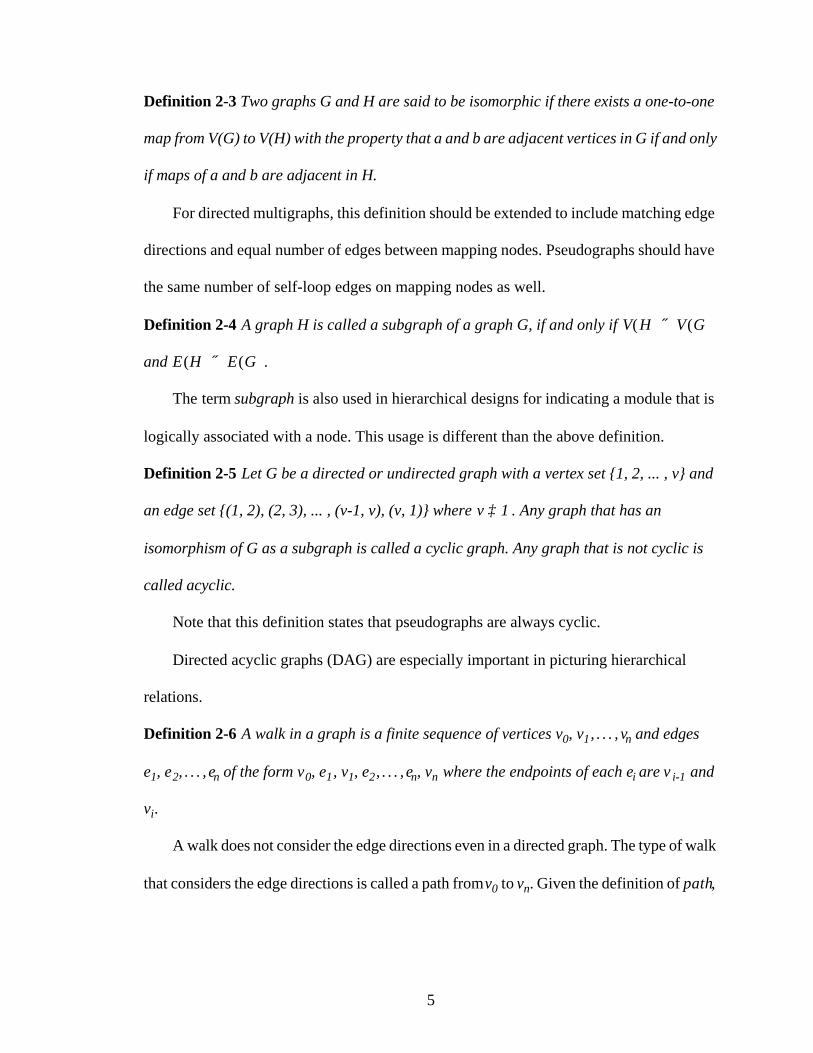
only one incoming edge. The one node with no incoming edge is called the root of the tree.
In a tree, the sink of an edge is called the child of the source. Vertices with no children are
called leaves of the tree.
Figure2-1 demonstrates examples graph types that are commonly mentioned in this
thesis: (a) A DAG (b) A directed cyclic graph (c) A tree.
There exist various ways to represent a graph in terms of a programming data structure.
The chosen structure often effects the efficiency of algorithms. Two commonly used data
structures for this purpose are adjacency lists and adjacency matrices. Both representations
only maintain references that contain the adjacency information of nodes. While this is a
very efficient method for basic graph algorithms, no compact data structure is provided for
Figure 2-1. Examples of graph types.
(a) (b) (c)
7
additional information that might be associated with nodes or edges. An alternative graph
representation in object-oriented languages is to assign an object to each node and edge, by
which all node and edge information can be stored in the hierarchy of objects.
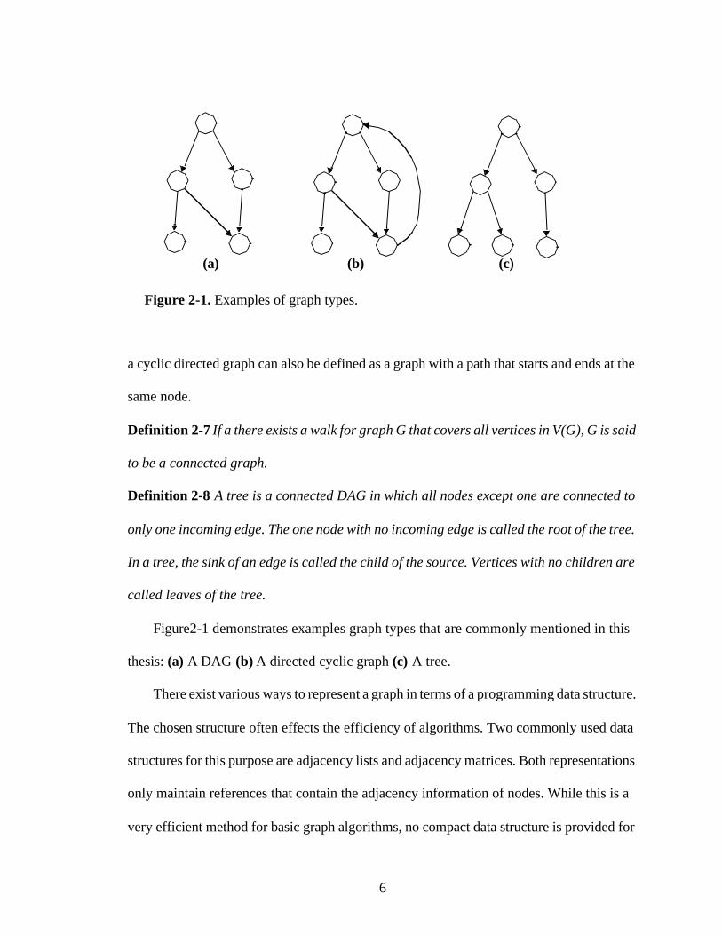
Depth First Tree Walk — Many applications, such as compilers, create a tree
representation of the input data and then process the nodes in the tree. The order of visiting
the nodes of a tree during the process is called a tree walk or a tree traversal. One of the
common tree traversals is the depth-first walk. In a depth-first walk, nodes are visited
following the edges. Starting from the root, the walk starts by going down to one of the
children and recursively continues, until a leaf is reached. After a leaf is reached the
algorithm walks back one step and checks if there are any unvisited nodes. If there are, the
walk continues down the unvisited new path, otherwise algorithm walks back until a node
with an unvisited child is found. The walk ends at the tree root when all the children of the
root are visited. Every node is visited twice during a depth-first walk: first during the down-
walk and second on the walk back. The tree-walks we will consider in this thesis will
Figure 2-2. Illustration of a depth first tree walk.
8
assume that always the leftmost unvisited child is selected as the next path to continue from.
Figure 2-2 illustrates a such tree-walk.
2.2 Dataflow Graphs
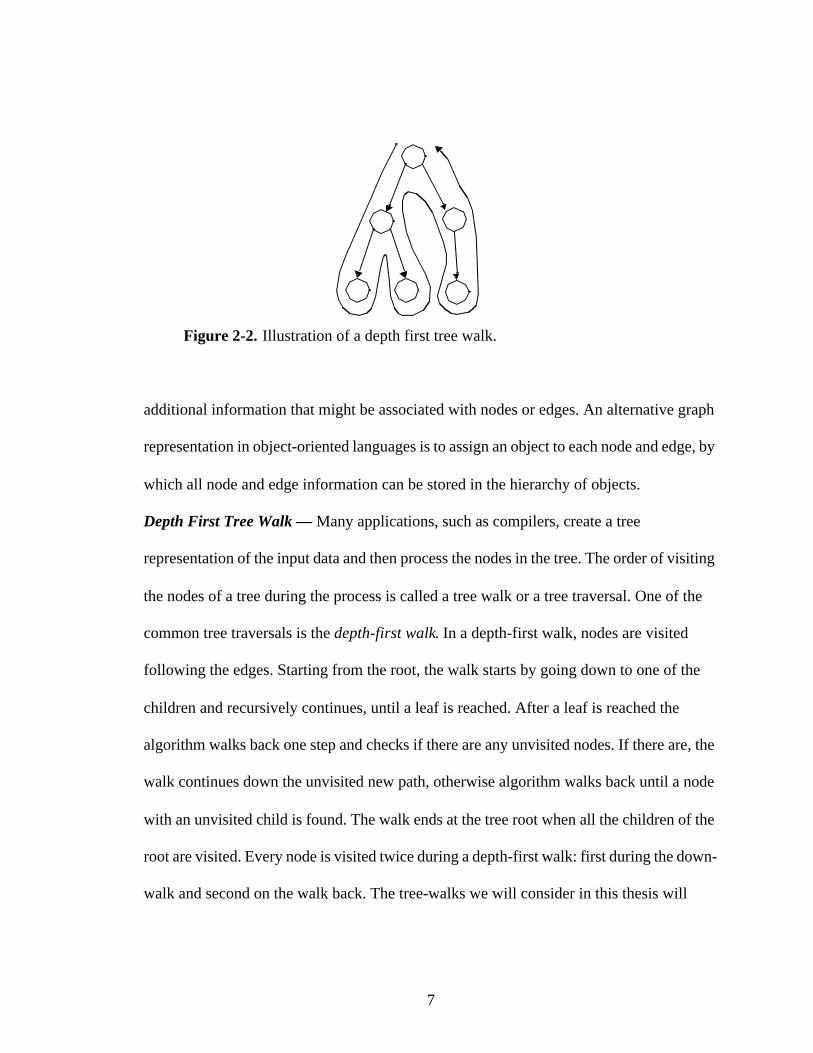
In dataflow programming model, a program is represented as a set of tasks with data
precedences. A dataflow graph consists of actors as nodes and unidirectional FIFO
channels as edges. In the semantics of dataflow graphs, actors consume, process (fire) and
produce data (tokens). The firing of actors is controlled by the actor firing rules. These rules
determine when enough data tokens are available to enable the actor. When firing rules are
satisfied, the actor fires, consumes a finite number of tokens and produces a finite number
of output tokens. Figure2-3 shows a dataflow graph in (a) and a firing example on (b).
Differences between dataflow graph types often involve production and consumption
rates. In the cyclo-static dataflow model [5], the numbers of tokens produced and consumed
by an actor can vary from one firing to the next in a cyclic pattern. In the synchronous
1 2
3
4
1 2
3
4
1 2
3
4
(a)
(b)
Figure 2-3. A dataflow graph example and firing of a dataflow graph.
9
dataflow model [12] the rates stay constant. Even more constrained cases are single rate
graphs [4] and homogeneous synchronous dataflow graphs (HSDF). Single rate graph
actors fire at the same average rate: production and consumption rates on an edge are equal.
In HSDF, this rate is set to unity.
2.3 Defining Formal Languages
A formal language is a set of finite length “strings”, over some finite alphabet. The
grammar of a formal language is a quadruple (N,T,R,S), where N is a finite set of
non-terminals, T is a finite set of terminal symbols, R is a finite set of productions, and
is the start symbol.
The set T of terminal symbols is also called the language alphabet. These symbols
both include the language keywords (see Section3.1.10 for a summary of DIF keywords),
operators and other separators. Non-terminals are symbols representing language
constructs. The set N should be disjoint from set T.
For context-free grammars, which DIF is a part of, productions are rules of the form
, where α is a non-terminal symbol and β is a string consisting of terminals or
non-terminals. The term context-free comes from the feature that α can always be replaced
by β, in no matter what context it occurs. The same α might appear at the left-hand side of
more than one production. The notational shortcut for this case is to use the | (pipe)
character to combine all such productions.
S N∈
α β→
10
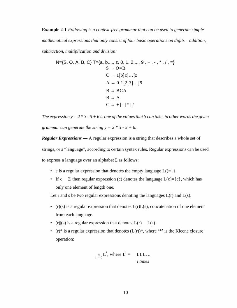
Example 2-1 Following is a context-free grammar that can be used to generate simple
mathematical expressions that only consist of four basic operations on digits – addition,
subtraction, multiplication and division:
N={S, O, A, B, C} T={a, b,..., z, 0, 1, 2,..., 9 , + , - , * , / , =}
The expression y = 2 * 3 - 5 + 6 is one of the values that S can take, in other words the given
grammar can generate the string y = 2 * 3 - 5 + 6.
Regular Expressions — A regular expression is a string that describes a whole set of
strings, or a “language”, according to certain syntax rules. Regular expressions can be used
to express a language over an alphabet Σ as follows:
• ε is a regular expression that denotes the empty language L()={}.
• If then regular expression (c) denotes the language L(c)={c}, which has
only one element of length one.
Let r and s be two regular expressions denoting the languages L(r) and L(s).
• (r)(s) is a regular expression that denotes L(r)L(s), concatenation of one element
from each language.
• (r)|(s) is a regular expression that denotes .
• (r)* is a regular expression that denotes (L(r))*, where ‘*’ is the Kleene closure
operation:
S O=B→O a b c … z→
A 0 1 2 3 … 9→
B BCA→B A→C + | - | * | /→
c Σ∈
L(r) L(s)∪
L i, where Li LLL…=i 0=
∞∪
i times
11
Frequently, regular expressions are extended with the following two operators.
• (r)+ is a regular expression that denotes L(r)L(r)*.
• (r)? is a regular expression that denotes .
Some additional rules are used in this thesis for conveniently expressing sets of ASCII
characters. Let x and y be two integers and a and b be two ASCII characters.
• R = x implies that R is the character with the ASCII code ‘x’.
• R = [x .. y] implies that R is the list of all characters with ASCII values starting
from x, up to and including y.
• R = [‘a’ .. ‘b’] (with single quotes around a and b) implies that R is the list of
ASCII characters starting from a, up to and including b, assuming that characters
are ordered according to their ASCII values.
• + and - characters, with no single quotes around, are used as the union and
exclusion operators on sets.
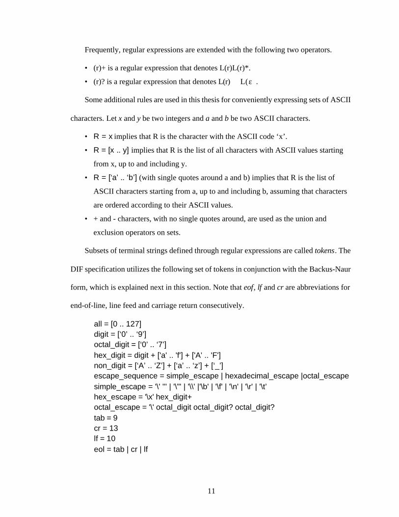
Subsets of terminal strings defined through regular expressions are called tokens. The
DIF specification utilizes the following set of tokens in conjunction with the Backus-Naur
form, which is explained next in this section. Note that eof, lf and cr are abbreviations for
end-of-line, line feed and carriage return consecutively.
all = [0 .. 127]digit = [‘0’ .. ‘9’]octal_digit = [‘0’ .. ‘7’]hex_digit = digit + ['a' .. 'f'] + ['A' .. 'F']non_digit = [‘A’ .. ‘Z’] + [‘a’ .. ‘z’] + [‘_’]escape_sequence = simple_escape | hexadecimal_escape |octal_escapesimple_escape = '\' ''' | '\"' | '\\' |'\b' | '\f' | '\n' | '\r' | '\t’hex_escape = '\x' hex_digit+octal_escape = '\' octal_digit octal_digit? octal_digit?tab = 9cr = 13lf = 10eol = tab | cr | lf
L(r) L(ε)∪
12
string = ‘”’ ([all - [‘”’ + ‘\’ + ‘cr’ + ‘lf’]] | escape_sequence)* ‘”’string_tail = '+' (' ' | eol | tab)* string
Backus-Naur Form (BNF) — BNF is a widely used syntax for defining languages with
context-free grammars. It was introduced by John Backus and was first used to describe the
syntax of the ALGOL 60 programming language [1]. BNF syntax is very similar to the
notation used in the formal languages part of this section. There are many variants and
extensions of BNF, one of which is the Extended BNF (EBNF). EBNF is enhanced with
regular expressions. In the DIF specification, regular expressions are integrated in EBNF
through tokens.
The following EBNF notation will be used for the formal definition of DIF:
• Language specific terminals, that are language keywords, operators and other
separators, will be printed in boldface. If the terminal is a single character, it will
appear between double quotes.
• Tokens, including strings, identifiers or numbers – see Section3.1.1 – are printed
as lightface plain text labels.
• Non-terminals will be expressed with a label enclosed between ‘<’and ‘>’
characters.
• The = character will be used to express a production.
• The | character will be used to combine alternative productions with the same left
hand side.
• The ‘+’, ‘*’ and ‘?’ operators of regular expressions can also be used with
non-terminals.
• The ‘[label]:’ notation may be used before terminals for descriptive purposes.
• The ‘{label}’ notation may be used before non-terminals for descriptive purposes.
The last two rules are not standard in BNF and they do not contribute to the language
definition. They are mainly defined for the reader’s convenience and compiler
compatibility, which will be described in Chapter4).
13
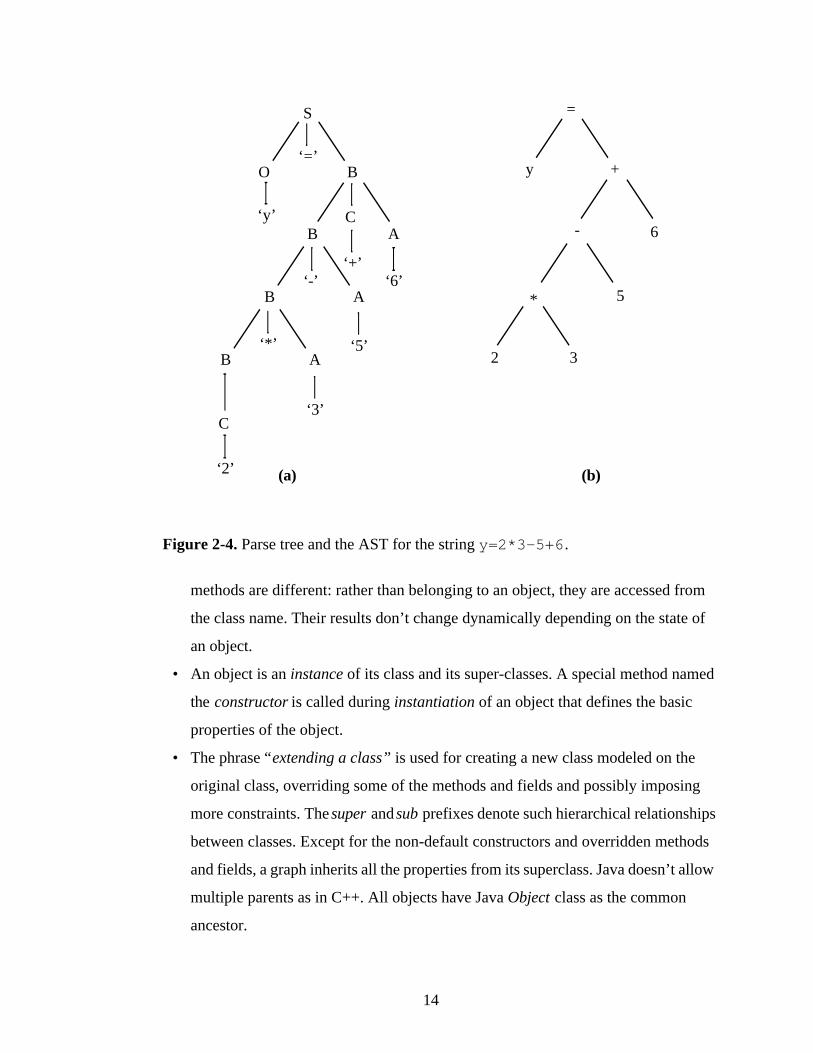
Syntax Trees — A parse tree pictorially shows how the start symbol of a grammar derives
a particular string in the language. Given a context-free grammar, a parse tree has the
following properties:
• The root is the start symbol.
• Each leaf is labeled by a token or by the empty string symbol ε.
• Each interior node is labeled by a non-terminal.
• If A is a non-terminal and X1, X2, ..., Xn are the children of node A (terminal or
non-terminal) ordered from left to right, this implies the production:
A slightly different version of parse trees is the Abstract Syntax Tree (AST), which
eliminates the non-terminals from the tree by replacing them with operators.
Example2-4 shows the (a) parse tree and the (b) AST for the string y=2*3-5+6
generated by the language in Example2-1.
Parse trees are often generated by the parser stage of compilers for processing the
tokens passed from lexer stage. The parse tree can be traversed in various ways depending
on the implementation and the desired transformation. The most common tree traversal is
the depth-first walk.
2.4 The Java Programming Language
Java [17] is a platform-independent, object-oriented programming language. The DIF
package is developed with Java. The following is a list of Java terminology that is used in
the subsequent chapters:
• In Java, object types are also named as classes. Functions are called methods and
variables are sometimes referred to as fields. Member methods and fields belong to
the instance of a class (or object) and they produce object specific results. Static
A X1X2…Xn→
14
methods are different: rather than belonging to an object, they are accessed from
the class name. Their results don’t change dynamically depending on the state of
an object.
• An object is an instance of its class and its super-classes. A special method named
the constructor is called during instantiation of an object that defines the basic
properties of the object.
• The phrase “extending a class” is used for creating a new class modeled on the
original class, overriding some of the methods and fields and possibly imposing
more constraints. The super and sub prefixes denote such hierarchical relationships
between classes. Except for the non-default constructors and overridden methods
and fields, a graph inherits all the properties from its superclass. Java doesn’t allow
multiple parents as in C++. All objects have Java Object class as the common
ancestor.
S
O B
BC
A
‘=’
‘y’
B A‘-’
B A‘*’
C
‘2’
‘3’
‘5’
‘+’
+
=
y
-
*
2 3
5
6
‘6’
(a)
Figure 2-4. Parse tree and the AST for the string y=2*3-5+6.
(b)
15
• A public method or a member can be accessed anywhere unlike protected methods
and members, which can only be accessed by package classes and subclasses. The
software convention used in this thesis enforces prefixing underscore “_” character
to protected method and member names.
• Errors are reported through classes called an exceptions. Usually, different kinds of
exceptions are thrown for different kinds of errors.
• Logically related classes can be collected in a single directory which is called a
Java package. The sub-packages of a Java package are physically stored in
sub-directories of the parent package. A full class name is represented in
package.sub-package.sub-sub-package...Class_Name
format. Packages do not impose any constraints other than a logical relationship
between classes, for example, classes of a sub-package do not necessarily extend
the classes of its super package.
• The period “.” operator in Java is used for accessing member fields and methods of
an object or static methods of a class. It is also used as the separator character in
full class names.
16
CHAPTER 3
Dataflow Interchange Format
DIF captures essential modeling information that is required in dataflow-based
analysis and optimization techniques, such as algorithms for consistency analysis,
scheduling, memory management, and block processing, while optionally hiding
proprietary details such as the actual code that implements the dataflow blocks.
DIF is designed to be exported and imported automatically by tools. However, unlike
other interchange formats, DIF is also designed to be read and written by designers who
wish to understand the dataflow structure of applications or the dataflow semantics of a
particular design tool, or who wish to specify an application model for one or more design
tools using the features of DIF. Indeed, DIF provides the programmer a unique, integrated
set of semantic features that are relevant to dataflow modeling. As a result, DIF is not based
on XML, which is more for pure data exchange applications, and is not well-suited for
being read or written by humans. Due to the emphasis on readability, DIF supports C and
Java-style comments, allows specifications to be modularized across multiple files
(through integration with the standard C preprocessor), and is based on a block-structured
syntax.
A dataflow graph definition in DIF consists in general of six blocks of code: topology,
interface, refinement, user-defined and built-in attributes, and parameters. These code
blocks are contained in a main block defining the dataflow graph. Using the basedon
keyword, a graph can inherit the same topology as another graph while overriding arbitrary
17
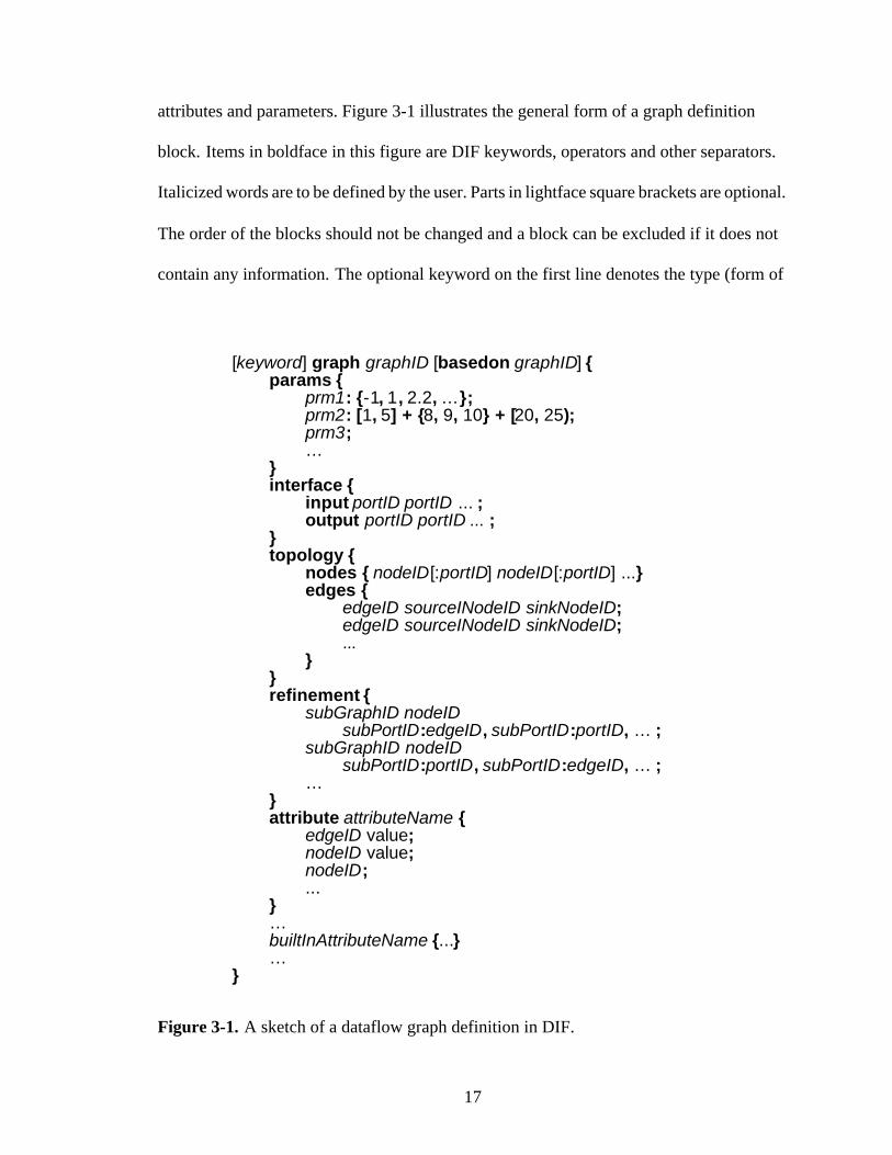
attributes and parameters. Figure 3-1 illustrates the general form of a graph definition
block. Items in boldface in this figure are DIF keywords, operators and other separators.
Italicized words are to be defined by the user. Parts in lightface square brackets are optional.
The order of the blocks should not be changed and a block can be excluded if it does not
contain any information. The optional keyword on the first line denotes the type (form of
[keyword] graph graphID [basedon graphID] {params {
prm1: {-1, 1, 2.2, …};prm2: [1, 5] + {8, 9, 10} + [20, 25);prm3;…
}interface {
input portID portID ... ;output portID portID ... ;
}topology {
nodes { nodeID[:portID] nodeID[:portID] ...}edges {
edgeID sourceINodeID sinkNodeID;edgeID sourceINodeID sinkNodeID;...
}}refinement {
subGraphID nodeID subPortID:edgeID, subPortID:portID, … ;
subGraphID nodeID subPortID:portID, subPortID:edgeID, … ;
…}attribute attributeName {
edgeID value;nodeID value;nodeID;...
}…builtInAttributeName {...}…
}
Figure 3-1. A sketch of a dataflow graph definition in DIF.
18
dataflow). Further details on the different graph types available are described in
Section3.2.
3.1 The Language
This section focuses on formally defining DIF in the context of programming
languages, providing detailed information on the syntax of the language. It also intends to
determine specifications of the required parsing functionality. An implementation of such
a parser is explained in Chapter 4.
3.1.1 Lexical Conventions
Syntactical basics of DIF are kept consistent with the syntax of popular programming
languages such as C and Java. Identifiers and numbers are defined in the same way as C.
Both block comments and line comments are supported.
DIF is a case sensitive language. Not using the correct type case for a language
keyword is a syntactical error. Literals with the same spelling but different type cases are
considered to represent different entities. White space characters, which are tabs, new lines
and form feeds, are ignored except when they separate identifiers, keywords and constants.
The tokens defined in this section are added to the tokens that were previously defined
for EBNF.
Numbers — Two types of numbers are used in DIF, signed integers or signed numbers
with decimal point (double). 1, 1.0, +0.7, -.9 are the examples of valid values.
double = (‘+’ | ‘-’)? (digit*) ‘.’ (digit+)integer = (‘+’ | ‘-’)? (digit*)number = double | integer
Identifiers — An identifier is a sequence of letters and digits. The first character must be a
letter or underscore. The maximum length of identifiers is not defined and usually bound
19
by the compiler implementation. Edge, node and attribute names in DIF are defined as
identifiers.
identifier = non_digit ( digit | non_digit )*
Comments — The characters /* introduce a block (long) comment, which terminates
with the characters */. The characters // introduce a line (short) comment, which
terminates with an end-of-line or end-of-file, whichever comes first. Comments do not nest,
and they do not occur within string or character literals.
not_cr_lf = all - [ cr + lf ]not_star = all - '*'not_star_slash = not_star -'/'short_comment = '//' not_cr_lf* eollong_comment = '/*' not_star* '*'+ (not_star_slash not_star* '*'+)* '/'comment = long_comment | short_comment
3.1.2 The Body of a DIF Specification
A DIF specification begins with an optional type keyword. Presently, the type
keywords include dif, sdf, csdf, singleRate and hsdf. This list is tentative and will be
updated with more keywords as the development on DIF advances.
A graph defaults to type dif if the type keyword is not specified. As a type, the dif
keyword implies the most generic type of dataflow graph supported by DIF. Using a
different type keyword usually requires supplying additional information via built-in
attributes or accepting the default values for those attributes.
Following the graph type and the graph keyword comes an optional basedon
statement. A basedon statement is used for inheriting base features from another graph and
in some ways it is analogous to the inheritance operator “:” in C++ or “extends” keyword
in Java.
20
A graph specification can have six types of blocks: parameter definitions, interface
declaration, topology definition, refinements and attribute definitions. Blocks should have
the same order as in this list. If a block does not contain any information, it can be excluded.
Two types of attribute definitions exist: built-in and user-defined. Multiple built-in and
user-defined attribute blocks in a graph are allowed.
Edge, node and port identifiers should be unique, for example it is erroneous to define
a node label that is already defined as an edge, node or port label. Likewise, an attribute
identifier should not be duplicated for using with another attribute.
Following is the EBNF for the highest level definition for a DIF object. The
non-terminals at the right hand side of block production will be defined in the subsequent
sections.
<graph_list> = <graph_block>*
<graph_block> =[type]:identifier? graph [name]:identifier <basedon>? “{” <block>* “}”
<basedon> = basedon identifier
<block> =
{params} params <params_body> |{interface} interface <interface_body> |{topology} topology <topology_body> |{refinement} refinement <refinement_body> |{fixed_attribute} identifier <attribute_body> |{attribute} attribute identifier <attribute_body>
3.1.3 Defining the Topology of a Graph
The topology definition of a graph consists of node and edge definition blocks, marked
by nodes and edges keywords. These define the sets of nodes and edges, and associate a
21
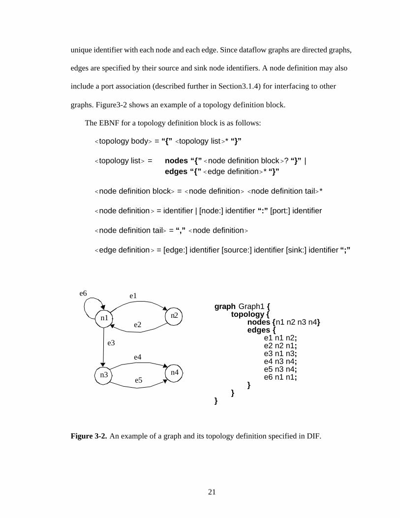
unique identifier with each node and each edge. Since dataflow graphs are directed graphs,
edges are specified by their source and sink node identifiers. A node definition may also
include a port association (described further in Section3.1.4) for interfacing to other
graphs. Figure3-2 shows an example of a topology definition block.
The EBNF for a topology definition block is as follows:
<topology body> = “{” <topology list>* “}”
<topology list> = nodes “{” <node definition block>? “}” |edges “{” <edge definition>* “}”
<node definition block> = <node definition> <node definition tail>*
<node definition> = identifier | [node:] identifier “:” [port:] identifier
<node definition tail> = “,” <node definition>
<edge definition> = [edge:] identifier [source:] identifier [sink:] identifier “;”
n3 n4
n1 n2
e1
e2
e3
e4
e5
graph Graph1 {topology {
nodes {n1 n2 n3 n4}edges {
e1 n1 n2;e2 n2 n1;e3 n1 n3;e4 n3 n4;e5 n3 n4;e6 n1 n1;
}}
}
Figure 3-2. An example of a graph and its topology definition specified in DIF.
e6
22
3.1.4 Hierarchical Graphs
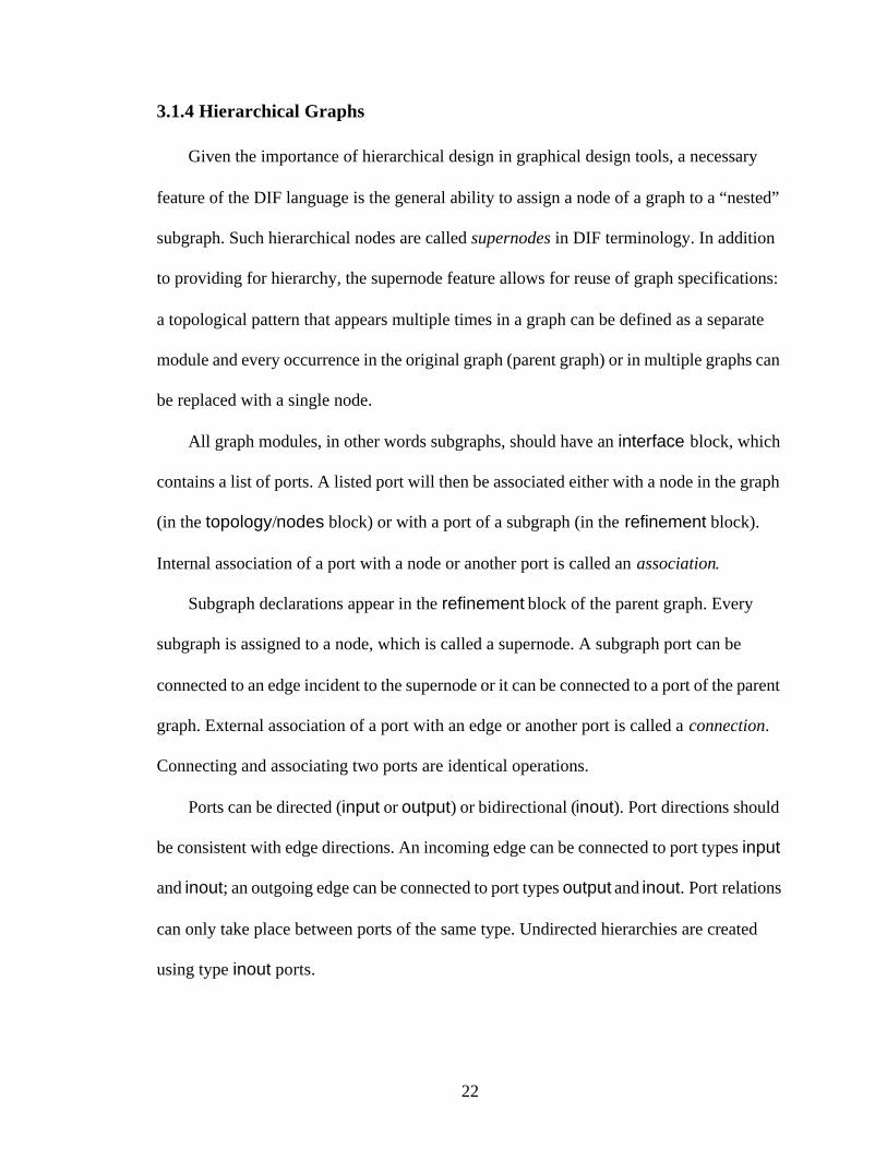
Given the importance of hierarchical design in graphical design tools, a necessary
feature of the DIF language is the general ability to assign a node of a graph to a “nested”
subgraph. Such hierarchical nodes are called supernodes in DIF terminology. In addition
to providing for hierarchy, the supernode feature allows for reuse of graph specifications:
a topological pattern that appears multiple times in a graph can be defined as a separate
module and every occurrence in the original graph (parent graph) or in multiple graphs can
be replaced with a single node.
All graph modules, in other words subgraphs, should have an interface block, which
contains a list of ports. A listed port will then be associated either with a node in the graph
(in the topology/nodes block) or with a port of a subgraph (in the refinement block).
Internal association of a port with a node or another port is called an association.
Subgraph declarations appear in the refinement block of the parent graph. Every
subgraph is assigned to a node, which is called a supernode. A subgraph port can be
connected to an edge incident to the supernode or it can be connected to a port of the parent
graph. External association of a port with an edge or another port is called a connection.
Connecting and associating two ports are identical operations.
Ports can be directed (input or output) or bidirectional (inout). Port directions should
be consistent with edge directions. An incoming edge can be connected to port types input
and inout; an outgoing edge can be connected to port types output and inout. Port relations
can only take place between ports of the same type. Undirected hierarchies are created
using type inout ports.
23
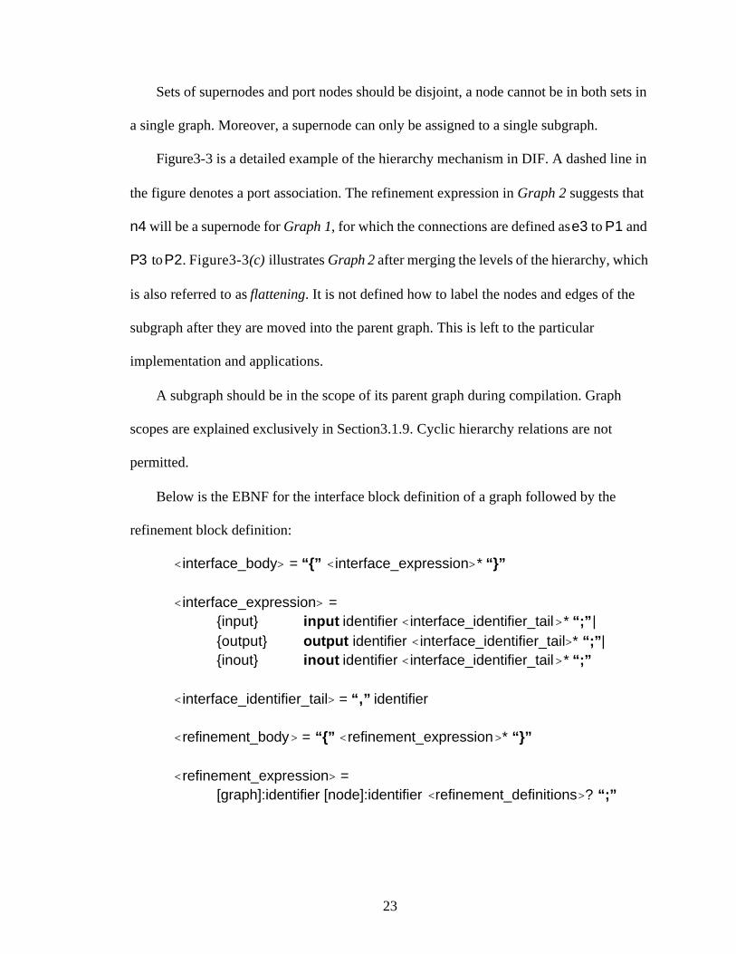
Sets of supernodes and port nodes should be disjoint, a node cannot be in both sets in
a single graph. Moreover, a supernode can only be assigned to a single subgraph.
Figure3-3 is a detailed example of the hierarchy mechanism in DIF. A dashed line in
the figure denotes a port association. The refinement expression in Graph 2 suggests that
n4 will be a supernode for Graph 1, for which the connections are defined as e3 to P1 and
P3 to P2. Figure3-3(c) illustrates Graph 2 after merging the levels of the hierarchy, which
is also referred to as flattening. It is not defined how to label the nodes and edges of the
subgraph after they are moved into the parent graph. This is left to the particular
implementation and applications.
A subgraph should be in the scope of its parent graph during compilation. Graph
scopes are explained exclusively in Section3.1.9. Cyclic hierarchy relations are not
permitted.
Below is the EBNF for the interface block definition of a graph followed by the
refinement block definition:
<interface_body> = “{” <interface_expression>* “}”
<interface_expression> ={input} input identifier <interface_identifier_tail>* “;”|{output} output identifier <interface_identifier_tail>* “;”|{inout} inout identifier <interface_identifier_tail>* “;”
<interface_identifier_tail> = “,” identifier
<refinement_body> = “{” <refinement_expression>* “}”
<refinement_expression> =[graph]:identifier [node]:identifier <refinement_definitions>? “;”
24
<refinement_definitions> =<refinement_connection> <refinement_connection_tail>*
<refinement_connection> = [port]:identifier “:” [element]:identifier
<refinement_connection_tail> = “,” [port]:identifier “:” [element]:identifier
n1 n2
P1 P2graph Graph1 {
…interface {
input P1, P2;}topology {
nodes {n1:P1 n2:P2}}…
}
n4
n3graph Graph2 {
…refinement {
Graph1 n4 P1:e2 P2:P3;}…
}
n1
n3P3
n2e1e2
(a)
(c)
Figure 3-3. Definition of DIF graphs with interfaces and super nodes.
e1
e2
P3
P1
P2
Graph1
Graph 2
(b)
Graph 2 after flattening
25
3.1.5 User-defined and Built-in Attributes
DIF supports assigning attributes to nodes, edges, and graphs. There are two types of
attributes: user-defined and built-in. User-defined attributes bear arbitrary names and can
take on any value assigned by the user. Built-in attributes are pre-defined with associated
keywords in the DIF language. They are usually handled in a special way by the compiler
and have default values even if they are not defined in the graph specification. Depending
on the particular semantics of a design tool and the type of the graph, a compiler might read
built-in attribute values into special fields of the edge-related data structures and it may
perform checks on the value to see if it is acceptable (e.g. positive-valued). An example of
a built-in attribute is the delay attribute of graph edges.
DIF supports four basic types of attribute values. Attribute types are not required to be
consistent within a single attribute block.
• Number An attribute value can be a signed integer or a signed double.
• 2-D Number Array This type is intended for defining matrices. However,
comparing rows for matching lengths is not a context-free language operation,
therefore the matrix property is not enforced in the formal language definition.
Instead, it is handled by the semantics analysis part following the parser. The syntax
of 2-D number array is rows of numbers separated by commas. An example is
(1 2 3, 4 5 6).
• List List is a very flexible type. Elements of a list can be of any type and types are
not required to match among elements. Even though the list type is defined to be
one dimensional, its elements can be other lists, which in effect enables lists of any
dimension. A list example is [[1, 2], [3, (4 5 6)], 7, 8].
• String C-language style strings are allowed in attributes. The concatenation
operator + can be used to collect multiple lines in a single string.
26
An attribute can also be parametrized, refer to Section3.1.6 for parametrization. The
EBNF for the attribute block definition is as follows:
<attribute_body> = “{” <attribute_expression>* “}”
<attribute_expression> ={element} identifier <value>? “;” |{graph} this <value>? “;”
<value> ={number} number |{param} identifier |{concat_string} string string_tail* |{array} “(” number* <array_row>* “)” |{list} “[” value+ “]”
<array_row> = “,” number*
If a value is not defined in an attribute expression, the particular attribute is undefined
for that element or graph. This is a feature that applies to graphs that are based on other
graphs. If the graph definition does not have a basedon statement, a empty-valued
attribute expression has no effect.
3.1.6 Parameters
Parameterization of attribute values is possible in DIF with the params block. The
capability of defining a possible set of values (domain) for an attribute instead of a specific
value provides useful support for analyzing dynamic and reconfigurable dataflow graphs.
The domain of a parameter can be an enumerated set of values, an interval, or a composition
of both forms. A parameter can be defined only once and the + character should be used for
combining different intervals. An example is prm1: {1, 2, 3.5} + [4, 5).
27
Parameters are defined in EBNF as follows:
<params_body> = “{”<params_expression>* “}”
<params_expression> ={normal} identifier “:” <range_block> “;” |{blank} identifier “;”
<range_block> = <range> <range_tail>*
<range> ={closed_closed} “[” [left]:number “,” [right]:number “]” |{open_closed} “(” [left]:number “,” [right]:number “]” |{closed_open} “[” [left]:number “,” [right]:number “)” |{open_open} “)” [left]:number “,” [right]:number “)” |{discrete} “}” number <discrete_range_number_tail>* “}”
<discrete_range_number_tail> = “,” number
<range_tail> = “+” <range>
3.1.7 The basedon Feature
DIF supports extending a graph definition to create a new graph object that inherits its
basic structure from the original model graph. This is a general property of object-oriented
languages and it is also suitable to DIF, which essentially defines objects, graphs, nodes and
edges, and defines their properties, attributes and parameters. The extended graph inherits
its final topology, interface, refinements and type from the model graph. It also inherits all
the parameters and attributes, however, overriding and extending these blocks with new
values and types are permitted.
Attributes can be undefined by leaving the value blank in a definition, which has no
effect if the attribute is not defined or the graph does not have a basedon statement. For
example, assume that Graph2 is based-on Graph1 and the user-defined size attribute is
28
assigned to node1 in Graph1. The following code will result in erasing the user-defined
size attribute from node1 of Graph2.
attribute size {node1;
}
A basedon graph should have its model graph in its scope. Section3.1.9 explains graph
scopes in detail. Cyclic basedon relations between graphs are not permitted.
3.1.8 Preprocessor Support
The DIF preprocessor is defined to be the same as the ANSI-C preprocessor as
specified in [16]. The include command of the preprocessor is particularly useful in
conjunction with the hierarchy and basedon mechanisms since it can be used to
conveniently add graphs to the scope of the current graph.
3.1.9 Scope of a Graph
Two cases in DIF require a graph to be present in the scope of another graph. The first
case occurs when a graph is basedon a model graph definition, requiring the model graph
to be in the scope of the extended graph . The second case is caused by the refinement
block. A subgraph should be in the scope of its parent.
There are two methods for including graph H in the scope of a graph G:
• Define H in the same text file following G,
• Use the include statement of the preprocessor.
29
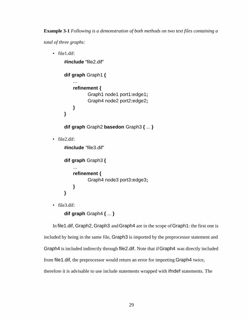
Example 3-1 Following is a demonstration of both methods on two text files containing a
total of three graphs:
• file1.dif:
#include “file2.dif”
dif graph Graph1 {...refinement {
Graph1 node1 port1:edge1;Graph4 node2 port2:edge2;
}}
dif graph Graph2 basedon Graph3 { ... }
• file2.dif:
#include “file3.dif”
dif graph Graph3 {...refinement {
Graph4 node3 port3:edge3;}
}
• file3.dif:
dif graph Graph4 { ... }
In file1.dif, Graph2, Graph3 and Graph4 are in the scope of Graph1: the first one is
included by being in the same file, Graph3 is imported by the preprocessor statement and
Graph4 is included indirectly through file2.dif. Note that if Graph4 was directly included
from file1.dif, the preprocessor would return an error for importing Graph4 twice,
therefore it is advisable to use include statements wrapped with ifndef statements. The
30
scope of Graph3 only includes Graph4, simply because graphs 1 and 2 are not referred to
from inside file2.dif, Graph4 does not have any graphs in its scope.
What paths to search and the order to search them for include statements are left to be
specified by the particular compiler implementation.
3.1.10 Summary of Keywords
Following is a list of keywords that are used in DIF grouped according to the places
they are used. The DIF language is case sensitive, therefore, special attention should be
paid to using the keywords with correct case.
• Top level definition: graph, dif, sdf, csdf, singleRate, hsdf.
• Topology definition: topology, nodes, edges.
• Interface declaration: interface, input, output, inout.
• Subgraph declarations: refinement.
• Parameter definitions: params.
• Attribute definitions: this
• User-defined: attribute
• Built-in: production, consumption, delay, transfer.
3.2 Supported Graph Types
The DIF language evolves in parallel with an accompanying the software package, the
DIF package, that is developed in University of Maryland. Even though this chapter deals
with language constructs that are implementation independent, many of the language rules
are shaped according to needs that arise during the development of the DIF package.
Especially, the supported graph types are open to such development, therefore this section
is dedicated to graph types with associated keywords and built-in attributes and
compatibility issues of graphs with other graphs for refinement definitions. All graph types
31
are assumed to be compatible with itself, meaning a graph can be a subgraph of another if
their types are the same.
3.2.1 DIF Graphs
DIF graphs are the default and most general class of dataflow graphs supported by
DIF. DIF graphs can be specified explicitly using the dif keyword. In DIF graphs, no
restriction is made on the rate at which data is produced and consumed on dataflow edges,
and other types of specialized assumptions, such as statically-known delay attributes, are
avoided as well. Hence an arbitrary attribute type can be attached to each node/edge
incidence to represent the associated dataflow properties. In the inheritance hierarchy of the
DIF intermediate representations, DIF graphs are the base class of all other forms of
dataflow. In this sense, all dataflow graphs modeled in DIF are instances of DIF graph.
Furthermore, if a tool cannot export to any of the more specialized versions of dataflow
supported by DIF, it should export to DIF graph. Naturally, a DIF graph can have all kinds
of graphs as subgraphs in its refinement definition.
3.2.2 CSDF Graphs
In restricted versions of the DIF graph model that are recognized in DIF, the numbers
of data values (tokens) produced and consumed by each node may be known statically and
edge delays may be fixed integers. For example, CSDF graphs, based on the cyclo-static
dataflow model [5], are specified by annotating DIF graph definitions with the csdf
keyword. In CSDF graphs, production and consumption rates can vary between node
executions, as long as the variation forms a certain type of periodic pattern. Consequently,
32
values of these rates are integer vectors. These vectors are associated with CSDF graph
edges using the production and consumption keywords. For example, the code fragment
production { e1 [1 1 2 4]; e2 [2 2 3]; }
associates the periodic production patterns
1, 1, 2, 4, 1, 1, 2, 4, ... and 2, 2, 3, 2, 2, 3, ...
with edges e1, and e2. If production, consumption and delay values are not defined for a
CSDF graph, default values are [1], [1], and 0 respectively. CSDF Graphs are compatible
with SDF, single rate and HSDF graphs in refinement definitions.
3.2.3 SDF Graphs
Similar to CSDF graphs, token production and consumption rates of synchronous
dataflow (SDF) graphs [12] are known at compile time, but they are fixed rather than
periodic integer values. SDF graphs are specified using the sdf keyword, and the arguments
of production and consumption specifiers in SDF graphs are required to be integers, as in:
production { e1 4; e2 3 ; }consumption { e1 5 ; e2 2 ; }delay { e1 1; e2 2; }
The last statement, which is permissible in other DIF graph types as well, associates
integer-valued delays to the specified edges. If production, consumption and delay values
are not defined for an SDF graph, default values are 1, 1, and 0 respectively. SDF graphs
can have single rate and HSDF graphs as their subgraphs.
3.2.4 Single Rate and HSDF Graphs
Single rate graphs are a special case of SDF graphs where the production and
consumption values on each edge are identical. In single rate graphs, nodes execute (“fire”)
at the same average rate. In the slightly more restricted case of homogeneous SDF (HSDF)
33
graphs, production and consumption values are equal to one for all edges. Instead of
production and consumption attributes, DIF uses the transfer keyword for edges in
single rate graphs. DIF does not associate an attribute for token transfer volume in HSDF
since it is not variable. The default transfer rate for single rate graphs is 1 and the default
delay for both single rate and HSDF graphs is 0. HSDF graphs can be defined as subgraphs
of single rate graphs.
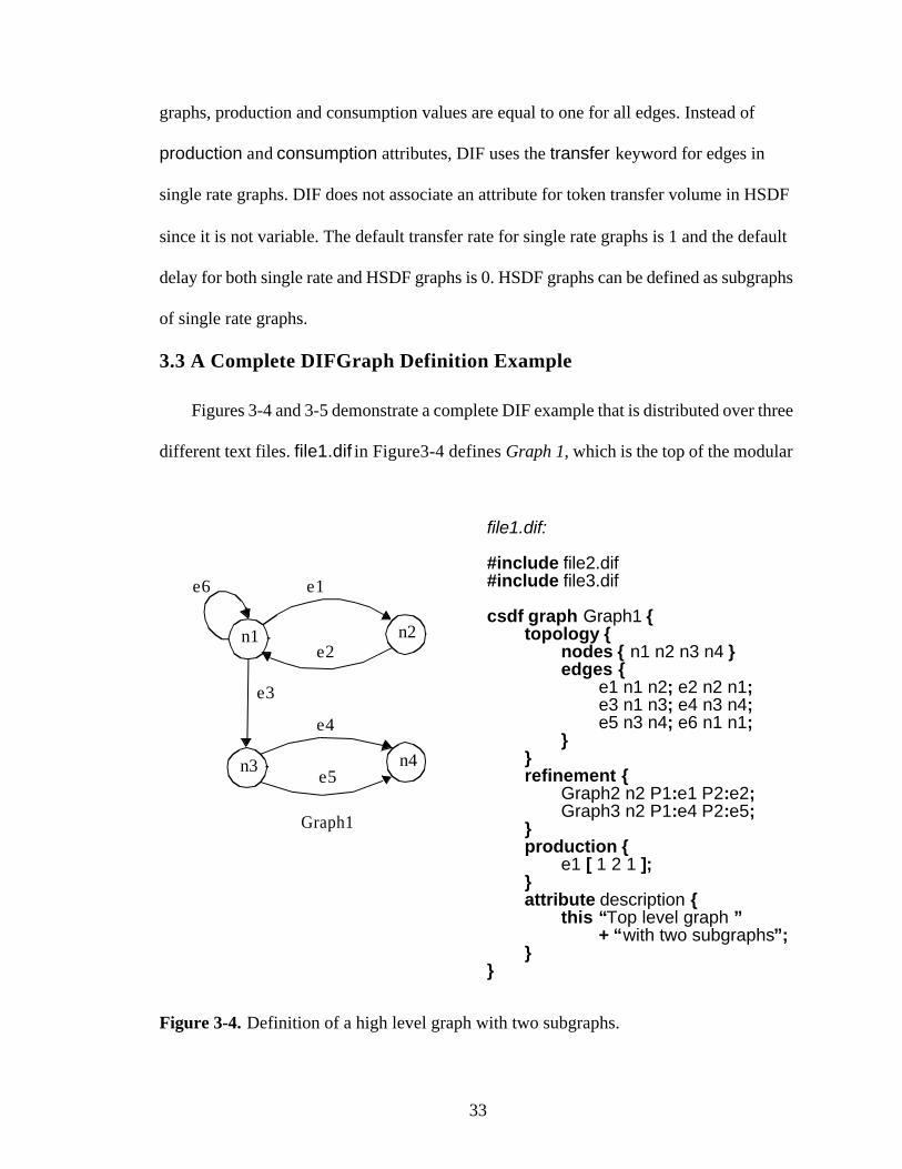
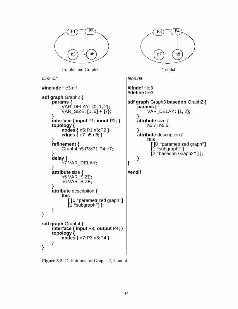
3.3 A Complete DIFGraph Definition Example
Figures 3-4 and 3-5 demonstrate a complete DIF example that is distributed over three
different text files. file1.dif in Figure3-4 defines Graph 1, which is the top of the modular
Figure 3-4. Definition of a high level graph with two subgraphs.
n3 n4
n1 n2
e1
e2
e3
e4
e5
e6
Graph1
file1.dif:
#include file2.dif#include file3.dif
csdf graph Graph1 {topology {
nodes { n1 n2 n3 n4 }edges {
e1 n1 n2; e2 n2 n1;e3 n1 n3; e4 n3 n4;e5 n3 n4; e6 n1 n1;
}}refinement {
Graph2 n2 P1:e1 P2:e2;Graph3 n2 P1:e4 P2:e5;
}production {
e1 [ 1 2 1 ];}attribute description {
this “Top level graph ”+ “with two subgraphs”;
}}
34
Figure 3-5. Definitions for Graphs 2, 3 and 4.
n5 n6
P1 P2
e7
Graph2 and Graph3
file2.dif:
#include file3.dif
sdf graph Graph2 {params {
VAR_DELAY: {0, 1, 2};VAR_SIZE: [1, 5] + {7};
}interface { input P1; inout P2; }topology {
nodes { n5:P1 n6:P2 }edges { e7 n5 n6; }
}refinement {
Graph4 n5 P3:P1 P4:e7;}delay {
e7 VAR_DELAY;}attribute size {
n5 VAR_SIZE;n6 VAR_SIZE;
}attribute description {
this [ [0 “parametrized graph”][1 “subgraph”] ];
}}
sdf graph Graph4 {interface { input P3; output P4; }topology {
nodes { n7:P3 n8:P4 }}
}
file3.dif:
#ifndef file3#define file3
sdf graph Graph3 basedon Graph2 {params {
VAR_DELAY: {1, 2};}attribute size {
n5 7; n6 5;}attribute description {
this[ [0 “parametrized graph”][1 “subgraph” ][2 “basedon Graph2” ] ];
}}
#endif
n7 n8
P3 P4
Graph4
35
hierarchy. Graph 1 requires Graphs 2 and 4 to be in its scope, therefore file2.dif and
file3.dif are imported within file1.dif. Graphs 2 and 4 are defined in file2.dif, which
automatically puts Graph 4 in the scope of Graph 2. Finally, Graph 3, which is based-on
Graph 2, is defined in file3.dif and file2.dif is imported to add Graph 2 to its scope. Note
that text in file3.dif is wrapped around by an ifndef preprocessor statement. Without this
statement Graph 4 would be imported twice in file1.dif: first, directly by the include
statement and then indirectly through file2.dif.
All edge production and consumption rates of Graph 1 are set to [1] by default, except
for the production rate of e1, which is set to the array [1 2 1]. A string attribute named
description is also defined for Graph 1. Two parameters are defined and used in Graph2,
one of which is overridden in Graph3.
36
CHAPTER 4
DIF Package
This chapter introduces the framework in which graph-based algorithms are developed
and presents the graph support tools in this framework. In Sections 4.2 and 4.4, internal
representations of topologies and hierarchies are discussed in detail, including low level
programming considerations. This discussion is followed by the introduction of the DIF
parser and writer in Sections 4.5 and 4.6, a front-end for converting DIF files to DIF API
objects and a writer for performing the reverse operation. In conclusion, an additional tool
for visualizing DIF graphs is explained and discussion about the content of the DIF package
is completed (Sections 4.7 and 4.8).
The software explained in this chapter is a subset of an infrastructure for system
synthesis research that is being developed by the DSP-CAD Research Group in the
University of Maryland at College Park. Generic graph representations used by this
package is maintained as a part of Ptolemy II, a set of Java packages supporting
heterogeneous, concurrent modeling and design. Ptolemy II is a part of the Ptolemy project
[11] conducted in University of California at Berkeley. The rest of the representations and
tools reside in the Maryland Package for System Synthesis (MAPSS).
The documentation in this chapter targets two kinds of users: developers and
non-developers. Non-developer users typically utilize the provided tools on supported
graphs but are not particularly interested in extending the DIF package for any purpose. On
the other hand, developers might heed to extend classes for unsupported graph types and
other features.
37
The DIF package is developed using the Java programming language. Extensibility of
classes and interface definitions of Java fit well to the layered software design of the DIF
package. Platform independence and inherent compatibility with graph notation through
object oriented programming are some of the other advantages of Java.
4.1 Organization of Classes
The inheritance hierarchy of dataflow graph types in the DIF API mimics the dataflow
graph type-hierarchy explained in Chapter 3 (e.g. CSDF graph is a constrained version of
directed graph and SDF graph is derived from CSDF graph with additional constraints, etc).
The careful design of the most generic graph type greatly facilitates the inheritance
hierarchy chain.
An example is the validNodeWeight method in the Graph class, which checks if a
weight object (see node in Section4.2.1) associated with a node is an acceptable type while
adding the node to a given graph.
public boolean validNodeWeight(Object object) {return true;
}
Clearly, this method will identify all node weights as valid. However, a graph type
such as DIFGraph that extends Graph, overrides the validNodeWeight method to require
a weight type, DIFNodeWeight, which is specifically defined for DIF graphs.
public boolean validNodeWeight(Object object) {return object instanceof DIFNodeWeight;
}
This is a top-down design methodology equipped by the detailed understanding of
similarities and differences of the class types that root from the generic graph. All segments
that might possibly deviate from the base class are modeled as methods that can be
38
overridden. The advantage of a thorough high level definition is the reduction in the
complexity of all extending classes and prevention of code duplication in many cases, for
example addNode methods do not need to be defined repeatedly in all subclasses since the
differences are captured in validNodeWeight method.
The convention used in the DIF package enforces a uniform use of protected and
public methods. Public methods are the complete set of functions that are needed by a
non-developer user, whereas protected methods are typically used for generic modeling
purposes as described above. Protected methods are occasionally used for communication
between closely coupled classes in the same Java package as well. Some modeling methods
may be defined as public for general convenience. The validNodeWeight method is one
such example: it is used internally for node verification and it is also set public so a user
can check and filter a set of node weights before adding them to a graph. The combined set
of public and protected methods form the developer API.
The logical structure of the Java packages in the DIF package generally follow the
hierarchy of the dataflow graph types. Different dataflow graph types are packaged
separately and placed into the package hierarchy according to their types. One addition to
the dataflow graph types is the DIFGraph which was explained in Chapter 3. The
DIFGraph class is developed with the purpose of enhancing the representation capabilities
of Graph objects for dataflow support, without changing the topological properties of basic
mathematical graphs. It is defined to be the most generic type of dataflow graph in the DIF
API. The DIFGraph class is equipped with an advanced data structure for storing dataflow
related parameters and attributes.
39
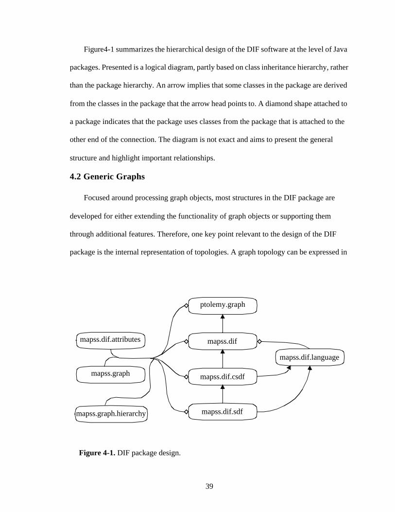
Figure4-1 summarizes the hierarchical design of the DIF software at the level of Java
packages. Presented is a logical diagram, partly based on class inheritance hierarchy, rather
than the package hierarchy. An arrow implies that some classes in the package are derived
from the classes in the package that the arrow head points to. A diamond shape attached to
a package indicates that the package uses classes from the package that is attached to the
other end of the connection. The diagram is not exact and aims to present the general
structure and highlight important relationships.
4.2 Generic Graphs
Focused around processing graph objects, most structures in the DIF package are
developed for either extending the functionality of graph objects or supporting them
through additional features. Therefore, one key point relevant to the design of the DIF
package is the internal representation of topologies. A graph topology can be expressed in
Figure 4-1. DIF package design.
ptolemy.graph
mapss.dif
mapss.dif.csdf
mapss.dif.sdf
mapss.dif.attributes
mapss.graph
mapss.dif.language
mapss.graph.hierarchy
40
more than one way as described in Section2.1 and the decision on how to represent graphs
directly affects the design of algorithms and procedures that operate on graphs.
For many of its representations and manipulations pertaining to generic graphs, DIF
employs the ptolemy.graph package from Ptolemy II [11].
4.2.1 Overview of Elementary Classes
This section gives an overview of major features from ptolemy.graph that are used in
DIF.
Following are the classes that are used for constructing basic directed and undirected
graphs. For the complete package documentation of the base graph package, refer to
Ptolemy II documentation.
Element — Element is a base class for the nodes and edges of a graph. Each node and edge
in a graph can optionally have a weight object associated with it. While element weights
are arbitrary objects in the base graph type, they are typically restricted for the classes that
extend Graph class. An element said to be weighted if it is assigned a weight and it is
referred to as unweighted otherwise.
Node — All vertices in a graph are instances of this simple class independent of directed
and undirected graph contexts.
Edge — All edges in a graph are instances of the Edge class. The connectivity of edges is
specified by source nodes and sink nodes. The graph model does not differentiate between
edge types of directed and undirected graphs. In the context of a directed graph, an edge is
directed from its source node to its sink node. In case of an undirected graph, there exists
no difference between source and sink nodes. This convenient notation simplifies the
logical conversion between directed and undirected graph types.
41
In support of pseudographs, self-loop edges and multiple edges between the same set
of nodes are allowed. Source and sink nodes of an edge are immutable: they cannot be
changed after being set.
Graph — This class models a graph with optionally-weighted edges and nodes, all of
which are instances of the Element class. A collection of edges and nodes does not form a
graph until all of them are added to a graph object, which inherently requires the edges and
the nodes of a graph to be unique. Both directed and undirected graphs can be implemented
using this class due to the combined support in the Edge class.
Each node (edge) is associated with a unique, integer label in a graph. These labels can
be used, for example, to index arrays and matrices whose rows/columns correspond to
nodes (edges).
A node or an edge can exist as an element in multiple graphs, but any given graph can
contain only one instance of the node. Node (or edge) labels, however, are local to
individual graphs. Thus, the same node may have different labels in different graphs.
Furthermore, the label assigned in a given graph to a node may change if the set of nodes
in the graph changes over time. As opposed to elements, weights of graph elements do not
need to be distinct. In other words, only one instance of an element can exist in a graph, but
distinct elements can share the same weight object.
If an edge will be removed from a graph and be re-added later, it can be hidden instead
of being removed from the graph. This method is more efficient than removing edges, in
terms of algorithm complexity and allows the same label to be used if the edge is restored
later.
42
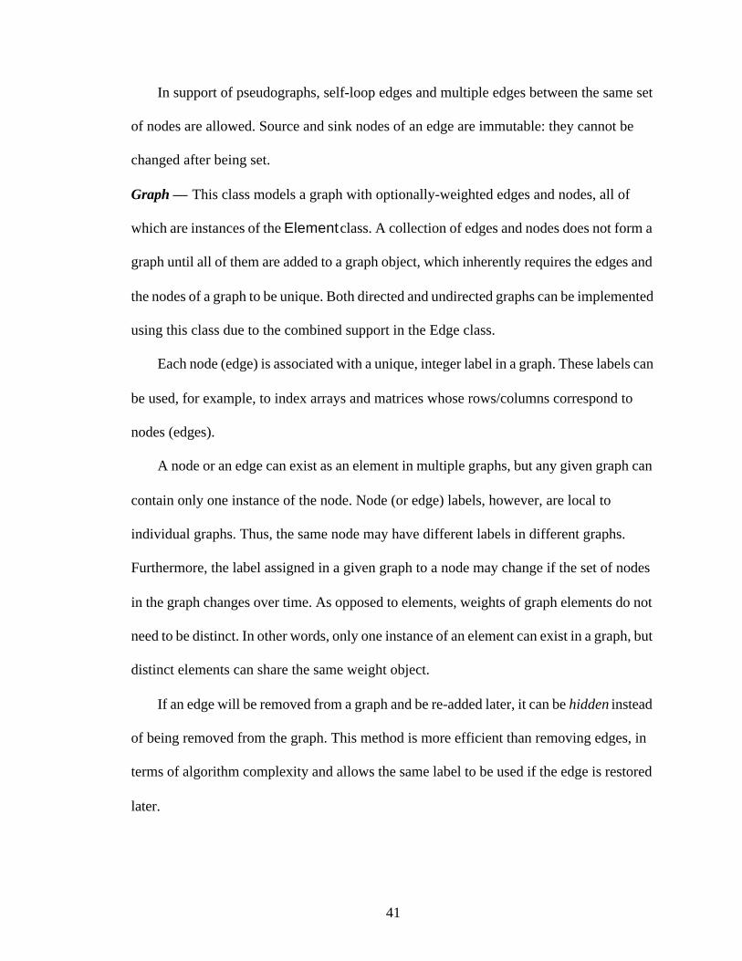
Directed Graph — The DirectedGraph class implements a transitive closure matrix,
which efficiently supports operations such as strongly connected component
decomposition, or finding reachable nodes. The transitive closure matrix is a boolean
matrix, whose indexes correspond to node labels. The entry is (i, j) true if and only if there
exists a path from the node with label i to the node with label j.
n3 n4
n1 n2
e1
e2
e3
e4
e5
e6
import ptolemy.graph.Graph;import ptolemy.graph.DirectedGraph;import ptolemy.graph.Edge;import ptolemy.graph.Node;
public class Example {
public Example ( ) {
// Construct the graph object.Graph graph = new Graph( );Node n1 = graph.addNode( );
...Node n2 = graph.addNode( );Edge e1 = addEdge(n1, n2);Edge e2 = addEdge(n2, n1);
...Edge e6 = addEdge(n1, n1);
// Convert to DirectedGraph and find transitive closure.DirectedGraph graph2 = grap.cloneAs(new DirectedGraph( ));boolean[ ][ ] matrix = graph2.transitiveClosure( );
}}
Transitive Closure=
1 1 1 01 0 0 00 0 0 10 0 0 0
Figure 4-2. An example of defining a basic graph.
43
Figure4-2 presents simple Java code that constructs the graph shown in the figure.
addNode and addEdge methods are shortcuts for instantiating weightless elements and
adding them to the graph. The graph is then copied into a DirectedGraph object which
provides a method to find the transitive closure matrix. Note that the cloneAs method
requires an empty graph of the desired type as a parameter to clone the current graph. Nodes
(and edges) are assigned integer labels starting from 0, in the order they are added to the
graph, which are used in the transitive closure matrix.
4.2.2 Cloning and Mirroring Graphs
Graphs can be copied by two methods: cloning and mirroring. Both methods produce
an isomorphic graph, however, they differ in the degree to which information is replicated.
Cloning — The clone of a graph uses the exact same element objects as the original graph,
thus original and clone graphs share the same node and edge objects. On the other hand, the
data structure that records the nodes and edges contained in the graph is copied.
Consequently, the Graph.equals method will return true for the clone and the original
graphs, unless the clone graph object is modified by adding, removing, hiding or restoring
elements.
The clone method has an extension that can be used to transform a graph into a
different type. The Graph.cloneAs method can clone a graph into a subtype of the original
graph. For instance, assume that a graph object is of type Graph,
DirectedGraph cloneGraph = graph.cloneAs(new DirectedGraph( ))
clones the graph object into a new object of type Directed Graph. The parameter in the
cloneAs method determines the graph type to clone as.
44
Mirroring — Mirroring a graph is effectively copying the complete data structure as
opposed to only copying the lists that record the edge and node objects in a graph. As a
result, the obtained graph object is not equal to the original graph when compared with the
Graph.equals method. The MirrorTransformerStrategy class of the
ptolemy.graph.analysis.strategy package should be used to mirror graphs. The same
class provides a method to search for a particular element that is mirrored from the original
class. The following is an example of mirroring a graph. Assume that graph is an object of
type Graph and e is an edge in graph.
MirrorTransformerStrategy transformer = new MirrorTransformerStrategy(graph);
Graph mirror = transformer.mirror( );Edge mirrorEdge = (Edge)transformer.transformedVersionOf(e);
It is optional to copy or share the weights between the elements of the original and the
mirror graphs. The default behavior is to share, which can partly be viewed as a protection
against non-cloneable weights.
4.3 The DIFGraph Class and mapss.dif Package
The DIFGraph class caches frequently-used data associated with generic dataflow
graphs and acts as the base class of an intermediate representation for performing dataflow
graph transformations , analyses, and optimizations.
The Attribute Mechanism
The attribute mechanism of the DIFGraph class can be used to bind arbitrary attributes
to elements or to the graph object itself. An attribute is an arbitrary object with a label
assigned to it. The object remains arbitrary even in sub-types of DIFGraph unlike weight
objects. There is no limit to the number of attributes an element or graph can possess.
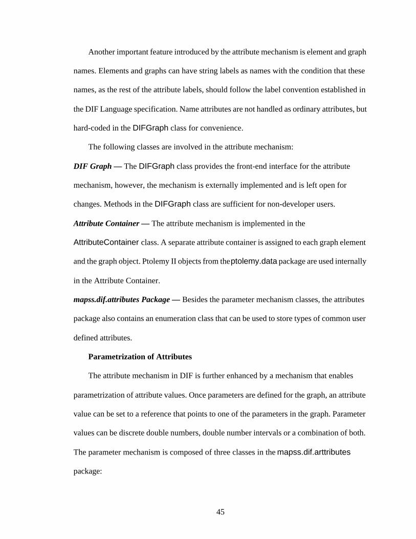
45
Another important feature introduced by the attribute mechanism is element and graph
names. Elements and graphs can have string labels as names with the condition that these
names, as the rest of the attribute labels, should follow the label convention established in
the DIF Language specification. Name attributes are not handled as ordinary attributes, but
hard-coded in the DIFGraph class for convenience.
The following classes are involved in the attribute mechanism:
DIF Graph — The DIFGraph class provides the front-end interface for the attribute
mechanism, however, the mechanism is externally implemented and is left open for
changes. Methods in the DIFGraph class are sufficient for non-developer users.
Attribute Container — The attribute mechanism is implemented in the
AttributeContainer class. A separate attribute container is assigned to each graph element
and the graph object. Ptolemy II objects from the ptolemy.data package are used internally
in the Attribute Container.
mapss.dif.attributes Package — Besides the parameter mechanism classes, the attributes
package also contains an enumeration class that can be used to store types of common user
defined attributes.
Parametrization of Attributes
The attribute mechanism in DIF is further enhanced by a mechanism that enables
parametrization of attribute values. Once parameters are defined for the graph, an attribute
value can be set to a reference that points to one of the parameters in the graph. Parameter
values can be discrete double numbers, double number intervals or a combination of both.
The parameter mechanism is composed of three classes in the mapss.dif.arttributes
package:
46
Parameter — Parameter is an inner class that serves as the parameter reference. A
parametrized attribute value is required to instantiate of this class.
Interval — This class represents a double number or a single interval with double number
boundaries. Each boundary can be defined to be inclusive or exclusive.
Interval Collection — The domain of a parameter value is modeled as a set of intervals.
All Intervals defined for a parameter are collected under a named IntervalCollection
object after going through some simple transformations such as merging with neighboring
intervals.
4.3.1 DIF Language Conversion from DIFGraph Objects
The DIFGraph class and other classes previously described in this section form the
infrastructure that is capable of importing the topology, parameter and attribute information
from a DIF specification without any data loss. An example of how a DIF specification can
be coded with the DIF package API is presented in Figures 4-3 and 4-4.
The DIF compiler and writer (see Sections 4.5 and 4.6) resolve some of the conversion
issues as follows:
• Element, graph, parameter and attribute names should be consistent with the DIF
specification of labels as explained in Section3.1.1. All such names in the DIF
package are checked by the mapss.util.Conventions class for errors. The default
check is consistent with the DIF specification, therefore no ambiguity exists during
conversions.
• User-defined attribute value types in the DIF language map to the following Java
objects in the DIF API: String, Double, 2-D double matrix – double[][] and List for
object arrays.
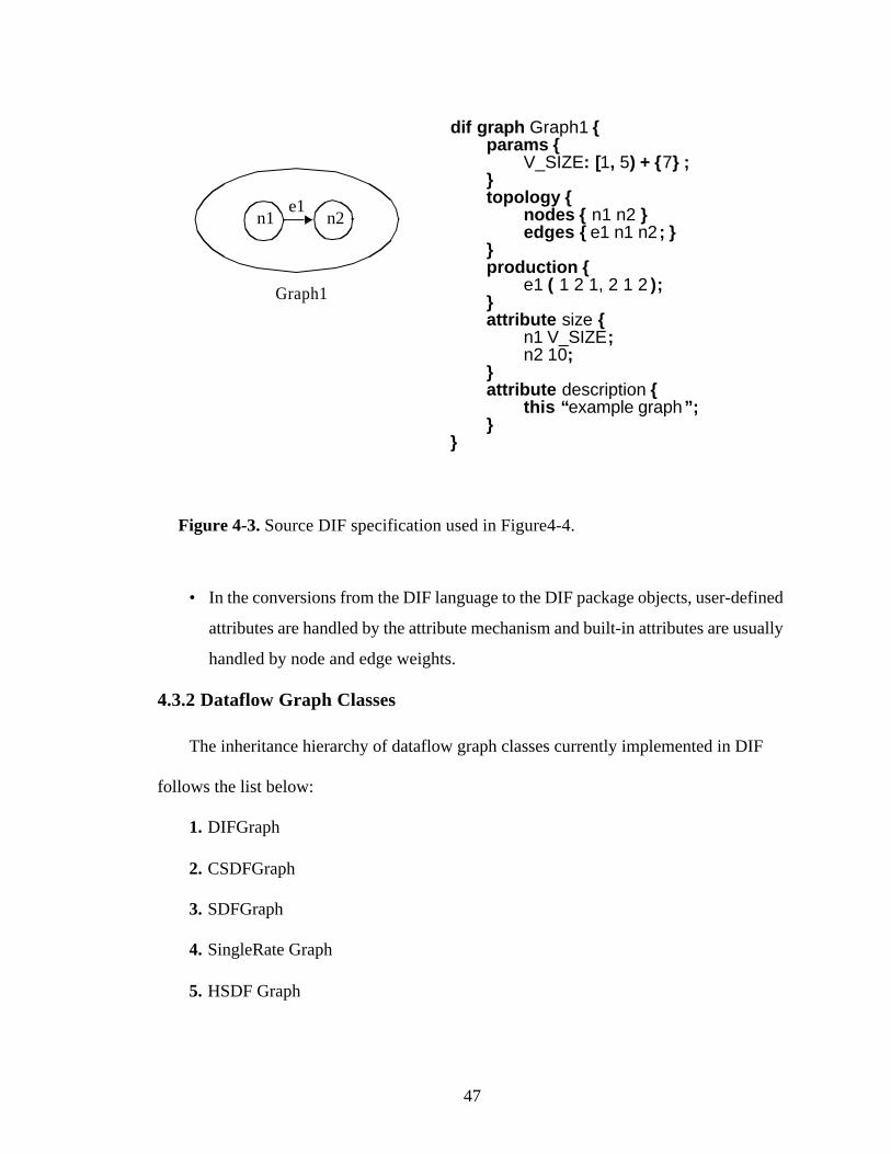
47
• In the conversions from the DIF language to the DIF package objects, user-defined
attributes are handled by the attribute mechanism and built-in attributes are usually
handled by node and edge weights.
4.3.2 Dataflow Graph Classes
The inheritance hierarchy of dataflow graph classes currently implemented in DIF
follows the list below:
1. DIFGraph
2. CSDFGraph
3. SDFGraph
4. SingleRate Graph
5. HSDF Graph
dif graph Graph1 {params {
V_SIZE: [1, 5) + {7} ;}topology {
nodes { n1 n2 }edges { e1 n1 n2 ; }
}production {
e1 ( 1 2 1, 2 1 2 );}attribute size {
n1 V_SIZE;n2 10;
}attribute description {
this “example graph”;}
}
n1 n2e1
Graph1
Figure 4-3. Source DIF specification used in Figure4-4.
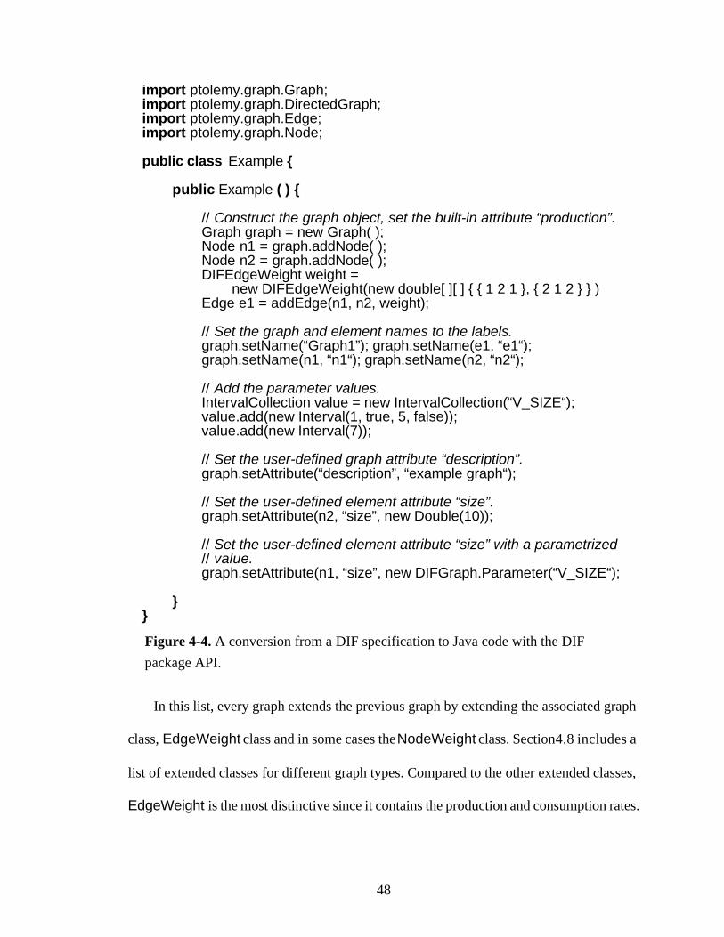
48
In this list, every graph extends the previous graph by extending the associated graph
class, EdgeWeight class and in some cases the NodeWeight class. Section4.8 includes a
list of extended classes for different graph types. Compared to the other extended classes,
EdgeWeight is the most distinctive since it contains the production and consumption rates.
Figure 4-4. A conversion from a DIF specification to Java code with the DIF package API.
import ptolemy.graph.Graph;import ptolemy.graph.DirectedGraph;import ptolemy.graph.Edge;import ptolemy.graph.Node;
public class Example {
public Example ( ) {
// Construct the graph object, set the built-in attribute “production”.Graph graph = new Graph( );Node n1 = graph.addNode( );Node n2 = graph.addNode( );DIFEdgeWeight weight =
new DIFEdgeWeight(new double[ ][ ] { { 1 2 1 }, { 2 1 2 } } )Edge e1 = addEdge(n1, n2, weight);
// Set the graph and element names to the labels.graph.setName(“Graph1”); graph.setName(e1, “e1“); graph.setName(n1, “n1“); graph.setName(n2, “n2“);
// Add the parameter values.IntervalCollection value = new IntervalCollection(“V_SIZE“);value.add(new Interval(1, true, 5, false));value.add(new Interval(7));
// Set the user-defined graph attribute “description”.graph.setAttribute(“description”, “example graph“);
// Set the user-defined element attribute “size”.graph.setAttribute(n2, “size”, new Double(10));
// Set the user-defined element attribute “size” with a parametrized// value.graph.setAttribute(n1, “size”, new DIFGraph.Parameter(“V_SIZE“);
}}
49
4.4 The Hierarchy Package
Modular design support is not provided directly through the Graph class. Instead,
subgraph information and hierarchical relations between graphs are captured in the classes
of the mapss.graph.hierarchy package, preserving the simplicity of the basic graph type.
The purpose of the Hierarchy package is to form a wrapper around Graph objects to
implement hierarchical graphs. Using this package, subgraphs can be defined within
graphs, nodes of a subgraph can be connected to its parent graph via ports and supernodes
(nodes that contain subgraphs) can be flattened to merge different levels of the hierarchy.
A hierarchy-enabled graph is called a hierarchy for brevity. The term subgraph is used
interchangeably with subhierarchy.
Defining a hierarchy requires two steps:
• Constructing a hierarchy object that contains the graph.
• Constructing the ports of the hierarchy object.
Once graphs are hierarchy enabled, they can be modularized. Following are the steps
for adding a subgraph to a graph:
• Assigning a node, called a super node of the super-graph, to the subgraph,
• Connecting the ports of the subgraph to edges or ports of the super-graph. Ports
can be directed or undirected. Undirected ports can be used as bidirectional ports.
A port can be connected to an edge or a port of its parent graph. It can also be
associated with a node or a subgraph port inside the graph. Figure 4-5 shows all the
schemes for port connections. Two possible connections, labeled as 1 and 2 in the figure,
and two possible associations, labeled as a and b, exist for a port. Connection 1 and
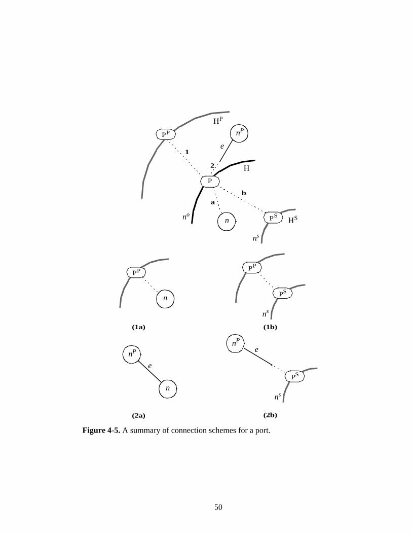
50
nP
e
n
P
PS
PP
2
1
ba
no
ns
nP
e
n
PP
n
PP
PS
ns
PS
ns
nP
e
(1a) (1b)
(2a) (2b)
Figure 4-5. A summary of connection schemes for a port.
H
HP
HS
51
association b are, in fact, identical, i.e. connection 1 is an association to port Pp and
association b is a connection to port PS.
Flatten methods are provided in the Hierarchy class for replacing super nodes with
their assigned subgraphs. This method places a mirror of the graph object into the parent
graph and removes the super node. Port connections are handled as shown in Figure4-5.
The top of the figure demonstrates all possible connections and relations on port P. Thick
lines denote graph boundaries. The letters P, n and e are used for ports, nodes and edges
respectively. Superscripts p and s are abbreviations for parent (outermost) graph and
subgraph (innermost graph), no is the label of the super-node that contains the graph
outlined by the dark contour and ns is the label of the super-node that contains the innermost
subgraph. Dotted lines represent port connections on the outside and port relations on the
inside. The sub-figures show how the connection and relations are resolved after flattening
the intermediate graph for different cases.
4.4.1 Overview of Classes
The hierarchy package contains six classes:
Hierarchy — Hierarchy is the wrapper class that stores the target graph in its data structure.
It provides methods to create, delete and flatten super-nodes among other methods, such as
clone and mirror.
Port — A hierarchy object interfaces with other hierarchies through Port objects. A port
belongs to the hierarchy object that is passed in its constructor. The port-hierarchy
association is immutable, meaning a port cannot be used as a port of another hierarchy after
it is created. The port class contains (dis)connect and (un)relate methods to handle
52
connections and a dispose method to remove it from the hierarchy. A disposed port cannot
be used any further.
Port List — PortList is an internal class that maintains the list of ports in a hierarchy. It
provides methods to check if a port label is previously defined or if an edge is connected to
another port prior to a connection. Unused port labels can safely be obtained through the
newName method. The order that the ports are added to this list is preserved in getAll and
iterator methods.
A port can be of types in, out or inout. Types in and out should be consistent with
directions of edges and ports that they are connected and related to. Type inout is
compatible with all directions, except that it can only be related to an inout type port.
Super Node Map — Super node map is another class internal to the hierarchy class. It
stores supernode/subhierarchy object pairs in a doubly-linked, ordered map. Due to the
double-link property both super-nodes and sub-hierarchies can be used as keys to obtain the
other pair from the map. The isDefined method is provided to check if a hierarchy name is
previously defined. Unused hierarchy names can safely be obtained through the newName
method. The order in which the pairs are added to this map is preserved in the getAll and
iterator methods.
Cyclic Hierarchy Exception — A cyclic hierarchy exception occurs if a nested hierarchy
definition is found to be cyclic, for instance a hierarchy cannot have itself as a subgraph. In
addition to being an exception type, this class provides a method to check if a subgraph
definition will create a cyclic relationship.
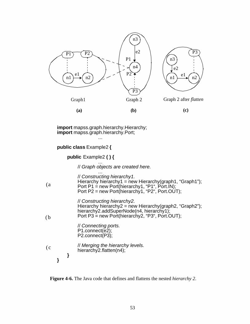
53
import mapss.graph.hierarchy.Hierarchy;import mapss.graph.hierarchy.Port;
...
public class Example2 {
public Example2 ( ) {...
// Graph objects are created here....
// Constructing hierarchy1.Hierarchy hierarchy1 = new Hierarchy(graph1, “Graph1”);Port P1 = new Port(hierarchy1, “P1“, Port.IN);Port P2 = new Port(hierarchy1, “P2“, Port.OUT);
// Constructing hierarchy2.Hierarchy hierarchy2 = new Hierarchy(graph2, “Graph2”);hierarchy2.addSuperNode(n4, hierarchy1);Port P3 = new Port(hierarchy2, “P3“, Port.OUT);
// Connecting ports.P1.connect(e2);P2.connect(P3);
// Merging the hierarchy levels.hierarchy2.flatten(n4);
}}
n1 n2
P1 P2
n4
n3
n1
n3P3
n2e1e2
(a)
e1
e2
P3
P1
P2
Graph1 Graph 2
(b)
Figure 4-6. The Java code that defines and flattens the nested hierarchy 2.
(c)
Graph 2 after flatten
b( )
c( )
a( )
54
Hierarchy Exception — All hierarchy related errors except the cyclic hierarchy error will
cause a hierarchy exception. Most of the error checking methods of the Hierarchy package
are defined in this class.
4.4.2 Hierarchy Related Functions
Hierarchical and topological structures of modular graphs are distributed over several
classes: Graph, Hierarchy, Port, etc. Consistency across these objects can be provided in
a strict or loose fashion. Strict consistency is accomplished by continuous verification. The
advantage of strict consistency is a persistently valid state, and the trade-off is close
coupling between all classes. This conflicts with the philosophy of the Hierarchy package,
which is to keep the hierarchy mechanism related code separate from the Graph class since
the latter is to be used purely for representing generic mathematical graphs. Therefore, the
loose-consistency scheme is found more suitable for DIF hierarchies. In the loose
approach, consistency verification is performed less frequently rather than with each
operation. In particular, graph operations, such as edge/node addition and removals are not
subject to any hierarchy related checks since there is no communication from the Graph
class to the Hierarchy class.
This section aims to describe how several functions in the Hierarchy package are
achieved while maintaining the desired loose consistency.
Adding a supernode to a hierarchy — Adding a supernode to a hierarchy only assigns a
subhierarchy with a node in the hierarchy. No connections or relations are defined at this
stage. The subhierarchy is removed from its previous parent, if it exists. The potential
supernode is unassigned from its previous subhierarchy as well. Then the supernode-
subhierarchy pair is added to the SuperNodeMap object in the Hierarchy and the parent
55
reference in the subhierarchy object is set. Before this procedure the following checks are
performed:
• The parent hierarchy does not contain another subhierarchy with the same name.
• The new supernode definition does not cause a cyclic relationship, i.e. the new
subhierarchy is not already an ancestor of the parent hierarchy.
Both of these properties cannot be violated once they are avoided at this step. Note that
the supernode is not checked to verify that it is a node in the parent graph, which is not an
essential check at this point since the node can later be removed from the graph.
The reverse of this process, called disconnecting, removes the parent reference in a
subhierarchy, removes the corresponding entry from the SuperNodeMap of the parent and
disconnects all the subhierarchy ports.
Defining a Port — A Port object is added to a Hierarchy through its constructor. In the
port constructor, the hierarchy reference and the name of the port is set and the port is added
to the PortList of the Hierarchy object. The hierarchy reference and the name field of the
Port class are immutable after they are created; a port can be removed from its hierarchy
but it cannot be used again (Port.dispose method). Also the port name is checked against
other port names in the hierarchy for uniqueness, a property that retains validity since port
names are immutable.
The Port.dispose method disconnects all connections and removes the PortList entry
in its hierarchy. Any attempt to use the member methods of a disposed port will result in an
error.
Connecting a port to an edge — The Port class provides a member method for
connecting an edge to a port object. It simply sets the connection field in the port,
56
overriding it if another connection is defined. When connecting e to P (see Figure4-5), the
following properties are verified.
• e is incident to n0
• If e is not a self-loop edge, it is not connected to another port of n0.
• If e is a self-loop edge, it is not connected to two other ports of n0.
• The direction of e matches the port direction: if n0 is the source of e, P should be of
type out, otherwise P should be of type in. If P is type inout both connections are
valid.
• If e is a self-loop edge and it is connected to two ports, both ports cannot be of type
in or type out at the same time.
Source and sink nodes of Edge objects are immutable, therefore the checks will
remain valid after the connection.
Associating a port to a node — Associate method in Port class first removes any previous
associations and then sets the node field in the Port object. No checks are performed in this
method.
Associating/connecting a port to another port — The port class contains both connect
and associate methods for ports. These methods are identical, for example, P.connect(PP)
has the same effect as PP.associate(P) where P is a port in the subhierarchy and PP is a
port in the parent hierarchy. During this connection, associatedPort and node fields of
PP and the connection field of P are set, overriding all previous field values. All ports in
overridden connections and associations are also disconnected/disassociated. Considering
the port connection (1) in Figure4-5, following statements are verified.
• H is a subhierarchy of HP.
• P and PP have the same directions or P is type inout.
Note that type inout ports cannot be related to type in or type out ports.
57
Flattening a supernode — Following is the algorithm for the Hierarchy.flatten function.
It is assumed that n0 in Figure4-5 is being flattened.
1. For all P store PSand n0.2. Add all edges and nodes in H to HP.3. Add all supernodes of H to HP:
Prefix all HS names with the name of H followed by a period “.”For all HS, store all port-edge connection pairs.Add all HS - ns pairs to the superNodeMap of HP.Restore edge connections for all HS.
4. For all P (ports of H) handle the connection/relation:connection = P.connectionN = P.nodeif connection is a Port
PP.unrelate( )if P is related to a node
PS.disconnect( )PS.connect(PP)
elsePP.relate(n)
else// Means connection is an edge.If relation is a node
Connect the edge to nelse
Connect the edge to ns
PS.connect(e)5. HP.disconnectSuperNode(n0)6. HP.removeNode(n0)
The steps labeled “Connect edge to ...” are not realizable in the Hierarchy API because
edges are immutable. The actual steps include instantiating new edges and replacing the old
edges with the new ones. Self-loop edges require special attention during this process.
Before the algorithm is run, the graph and the hierarchy objects are verified for
consistency. If an error is found, they are returned with no modification. An alternative is
calling the Hierarchy.purge method in advance to remove all faulty connections and
58
associations. After the purge method is run the Hierarchy object is guaranteed to be free of
errors. Below are the conditions that should be verified before flattening.
• n0 is a node in the graph of HP and n0 is a supernode in HP .
• All ports P of H are connected and related. All related nodes n or nS are elements
in the graph of H. All connected edges e are edges in the graph of HP.
4.4.3 Extending the Hierarchy Class
The Hierarchy class can be extended for handling different kind of graphs. Even
though most methods do not depend on the type of the backing graph object, mirror and
flatten methods require graph specific information. All extending classes should provide at
least one constructor with exactly two parameters: the graph and the name of the graph. The
_copyEdge method should be overridden to return an edge with the correct weight object
type, the _mirrorGraph method should return a MirrorTransformerStrategy object that
mirrors the backing graph in the desired way and the _graphType method should return
an empty graph with the graph type supported by this hierarchy.
4.4.4 DIF Language Conversion from DIFHierarchy Objects
The mapss.dif.language.Writer class can be used to write a DIFHierarchy object
into a DIF text file. This class is discussed in Section4.6. All port labels and the hierarchy
name are kept consistent with the DIF conventions. If the hierarchy name is different than
the graph name, the graph name is ignored.
4.5 The DIF Compiler
The DIF API provides a complete parser that translates DIF language text into graph
and hierarchy objects. This parser is automatically generated by the SableCC [7], a
compiler-compiler for building compilers in the Java programming language.
59
Parser related classes and packages are managed under mapss.dif.language. The list
of these classes are is follows:
• SableCC/compiler.Grammar SableCC language specification file for DIF.
• SableCC subpackages node, lexer, parser and analysis packages compose the
SableCC generated compiler framework.
• Language Analysis Contains the action code for compiling default DIF graphs.
New graph types are added to the compiler API by extending this class. This will be
covered in Section 4.5.3.
• analyzers.txt Contains the list of full names of default language analysis classes.
All default graph types in DIF are associated with an entry in this list. If a class is
not found in the JVM path or if an error occurs during initialization of a language
analysis, the corresponding graph type will be ignored from subsequent
compilations. Whitespaces and line or block comments in analyzers.txt are
ignored.
• Reader Front-end compiler interface. Accommodates the preprocessor, lexer and
parser functions. Compiled objects are accessed through getGraphs and
getHierarchies methods of this class.
• Graph Modifier A mini-compiler for reduced DIF language files. A reduced DIF
graph definition contains only a params block and attributes. It is very similar to
the basedon feature in regular DIF files except the graph to be modified is externally
loaded in the GraphModifier class.
• DIF Language Exception Thrown in case of language related errors.
4.5.1 SableCC
This section is a tutorial on SableCC features that were used in the design of the DIF
parser. As opposed to being a complementary guide, some features of SableCC are
deliberately ignored for brevity purposes. Refer to [7] for an complete tutorial.
SableCC employs the Visitor Design Pattern and takes advantage of the Java type
system to deliver modular, abstract syntax tree (AST) based, object-oriented compilers.
60
SableCC does not require any action code in specification files, rather it builds the
framework, in which actions can be added as Java code. Aside from ease of debugging, this
approach benefits from another major advantage: More than one compilers for the same
language can share a common framework. For example, the DIF package contains a
mini-compiler for reduced DIF, GraphModifier, in addition to the main compiler class.
DIF Parser Design with SableCC
The DIF parser was designed in five major steps:
1. The lexicon and the grammar of the language was defined in a SableCC
specification file.
2. The framework was generated by SableCC.
3. Action code was defined in the working-class, LanguageAnalysis, utilizing the
SableCC generated AST objects.
4. The main compiler class, Reader, was created to activate the lexer, the parser and
the analysis functions.
5. The parser was compiled with Java.
The steps of the design flow with the files or subpackages involved are illustrated in
Figure 4-7. Each step in the figure is numbered according to the list above.
The Language Specification File
SableCC language specification input is written in EBNF. As a result, the specification
file given in AppendixB is almost identical to the language specification in AppendixA.
The only major difference is that the specification file of SableCC contains another section,
that is helpers. Helpers are logical macros for using in the tokens section. Unlike text
macros, regular expressions in helpers are evaluated before substitution.
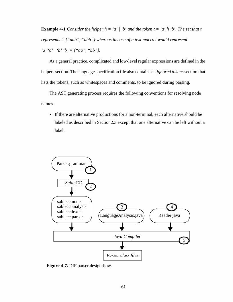
61
Example 4-1 Consider the helper h = ‘a’ | ‘b’ and the token t = ‘a’ h ‘b’. The set that t
represents is {“aab”, “abb”} whereas in case of a text macro t would represent
‘a’ ‘a’ | ‘b’ ‘b’ = {“aa”, “bb”}.
As a general practice, complicated and low-level regular expressions are defined in the
helpers section. The language specification file also contains an ignored tokens section that
lists the tokens, such as whitespaces and comments, to be ignored during parsing.
The AST generating process requires the following conventions for resolving node
names.
• If there are alternative productions for a non-terminal, each alternative should be
labeled as described in Section2.3 except that one alternative can be left without a
label.
Parser.grammar
SableCC
sablecc.nodesablecc.analysissablecc.lexersablecc.parser LanguageAnalysis.java Reader.java
Java Compiler
Parser class files
Figure 4-7. DIF parser design flow.
1
2
3 4
5
62
• If the same token is used more than once in a production, each token should be
labeled as described in Section2.3, except that only one token can be left
unlabeled.
SableCC generates four subpackages to build the compiler framework in the second
step of compiler design: lexer, parser, nodes and analysis. Among these, nodes and
analysis packages are used in the action code definition.
• nodes package This package contains the classes that represent the nodes of the
AST. Naming conventions for the parse tree are as follows
– A node representing an unnamed alternative of a production, is named by the
production name, prefixed with an uppercase “A”, first letter replaced by an
uppercase, each letter following an underscore replaced with an uppercase and
all underscores removed.
– Named alternatives translate into similar node names except, the alternative
label is placed between the “A” and the production name after the alternative
label goes through the same underscore conversion process.
– Named and unnamed tokens follow the preceding two rules with a minor
difference that “T” is used as the first letter.
AST noes are also equipped with accessor methods that return their children
tokens in the tree.
• analysis package The analysis package provides the tree traversal classes for
implementing the action code. The LanguageAnalysis class extends
analysis.DepthFirstAdapter for a depth first traversal on the AST. It also inherits
a list of node visitor methods, two for each node, which are called by the parser
during the first visit and the second visit of a node. These methods are overridden
by LanguageAnalysis to implement the action code for nodes. Node objects are
passed to the corresponding visitor methods as parameters, this is how the
LanguageAnalysis class interacts with the nodes package and accesses the token
strings. Visitor method names are obtained from the name of the corresponding
node object by adding one of the suffixes in (for the first visit) and out (for the
second visit).
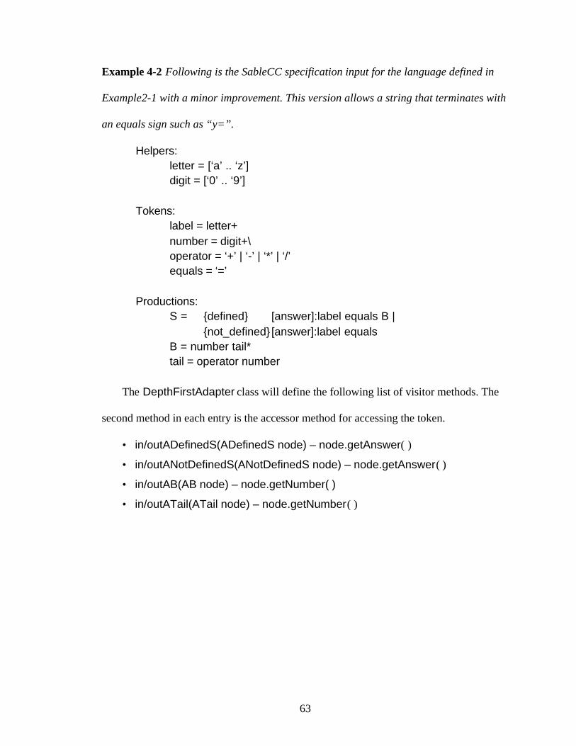
63
Example 4-2 Following is the SableCC specification input for the language defined in
Example2-1 with a minor improvement. This version allows a string that terminates with
an equals sign such as “y=”.
Helpers:letter = [‘a’ .. ‘z’]digit = [‘0’ .. ‘9’]
Tokens:label = letter+number = digit+\operator = ‘+’ | ‘-’ | ‘*’ | ‘/’equals = ‘=’
Productions:S = {defined} [answer]:label equals B |
{not_defined} [answer]:label equalsB = number tail*tail = operator number
The DepthFirstAdapter class will define the following list of visitor methods. The
second method in each entry is the accessor method for accessing the token.
• in/outADefinedS(ADefinedS node) – node.getAnswer( )
• in/outANotDefinedS(ANotDefinedS node) – node.getAnswer( )
• in/outAB(AB node) – node.getNumber( )
• in/outATail(ATail node) – node.getNumber( )
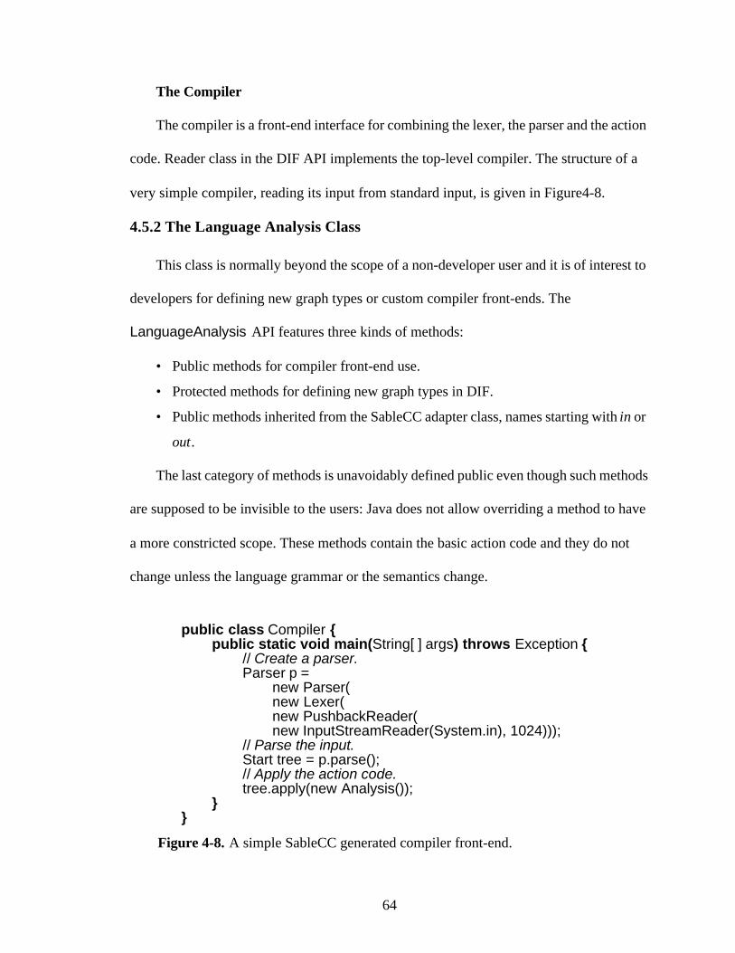
64
The Compiler
The compiler is a front-end interface for combining the lexer, the parser and the action
code. Reader class in the DIF API implements the top-level compiler. The structure of a
very simple compiler, reading its input from standard input, is given in Figure4-8.
4.5.2 The Language Analysis Class
This class is normally beyond the scope of a non-developer user and it is of interest to
developers for defining new graph types or custom compiler front-ends. The
LanguageAnalysis API features three kinds of methods:
• Public methods for compiler front-end use.
• Protected methods for defining new graph types in DIF.
• Public methods inherited from the SableCC adapter class, names starting with in or
out.
The last category of methods is unavoidably defined public even though such methods
are supposed to be invisible to the users: Java does not allow overriding a method to have
a more constricted scope. These methods contain the basic action code and they do not
change unless the language grammar or the semantics change.
public class Compiler {public static void main(String[ ] args) throws Exception {
// Create a parser.Parser p =
new Parser(new Lexer(new PushbackReader(new InputStreamReader(System.in), 1024)));
// Parse the input.Start tree = p.parse();// Apply the action code.tree.apply(new Analysis());
}}
Figure 4-8. A simple SableCC generated compiler front-end.
65
The remainder of the public methods, externalHierarchies, getHierarchy and
getKeyword are utilized by the compiler front-end. The compiler provides previously read
graphs to the parser through the externalHierarchies method. These graphs build the
scope of the graph being parsed.
Protected methods in LanguageAnalysis constitute a generic API for defining new
graph types in DIF. This is covered in detail in the next section.
4.5.3 Extending the DIF Language For A New Graph Type
In DIF, the differences between graph types typically arise from built-in attributes.
Therefore a new graph type definition mainly consists of new built-in attribute definitions.
A new graph type is introduced in two steps:
1. Extending the LanguageAnalysis class and overriding the following list of
methods:
– getEmptyXXX methods return an empty graph/edge/node that is of the type
that the input topology will be converted to.
– getKeyword returns the keyword for the new graph type.
– acceptableSubHierarchy(DIFHiearchy hierarchy) returns true if
hierarchy can semantically be a subhierarchy of the parsed graph.
2. Writing the action code to process fixed attributes. _processFixedAttributes
method should be overridden with appropriate code for each for each type of built-
in attribute. This method returns false if the attribute cannot be processed, which
will induce an error thrown by compiler.
3. Adding the full name of the new analysis to analyzers.txt.
66
4.5.4 The Reader Class – The Front-End Compiler
The reader class of the DIF compiler is more advanced than the front-end in Figure4-
8. Default graph analyzers listed by analyzers.txt are initialized by Reader. If desired,
custom analyzers can be added through the compile method. The Reader class also
contains the preprocessor mechanism of DIF, which is implemented through a system call
to the GNU C preprocessor.
A DIF file is compiled by passing the input file name in the constructor, running the
compile method and calling the getGraphs or getHierarchies methods for the output.
Following is an informal pseudocode that explains the compile method of Reader. It
is assumed that all analyzers are read into a list analyzers during initialization and also cpp
is a function that runs the preprocessor on the input. The cpp function reads all the files
indicated by the include statements and creates an ordered map of the file names to the DIF
file texts. The keys are ordered from the most dependent file to the files with no include
statements. This means that given any entry on the list; the scope of the file in the entry
consists of the subsequent entries in the list. For this reason, the list is compiled in reverse
order.
FUNCTION: Reader Main FunctionINPUTS: analyzers: LanguageAnalysisList, fileName: StringRETURNS: hierarchies: DIFHierarchyList
files = cpp fileName// Start reading files from the least dependent one.for (name, text) in files following reverse order
// Pass each text through lexer & parser for error check.// If error check is performed later, file names and line // numbers will be lost and errors will be harder to// track by the user.parser lexer text
←
← ←
67
for graphText in test following orderif graphText.keyword == null then
graphText. keyword = difanalyzer = analyzers.find(keyword)if “basedon modelName” exists in graphText
if modelName == graphText.name thenthrow "Graph cannot be based on itself"
modelObj = hierarchies.find(modelName)if modelObj == null then
throw "Model graph not found"mirrorObj = modelObj.mirror( )GraphModifier.modify(mirrorObj, graphText)hierarchies.add(mirrorObj)
else// All semantic checks on the input is performed// by the analyzer in the action-code.graphObj = analyzer parser lexer texthieracrchies.add(graphObj)
return hierarchies
4.6 The DIF Writer
DIF conversion considerations involving DIFGraph and Hierarchy objects were
discussed in Sections 4.3.1 and Section4.4.4. The DIFWriter class follows the guidelines
provided in those sections. Following is a partial list of DIF Language constructs in
Figure 3-1 and the methods they are obtained from in DIFWriter. Types of the values
returned by some of the methods are indicated in italic font.
keyword DIFWriter._graphType( )graphID DIFGraph.getName( )prmi List DIFGraph.getParameterNames( )parameter values
IntervalCollection DIFGraph._getParameterValue(prmi)IntervalCollection.toString( )
← ← ←
→ →
→ →
68
portID PortList Hierarchy.getPorts( ) and Port class methodsnode/edgeID DIFGraph.getName(node/edge)refinement block SuperNodeMap Hierarchy.getSuperNodes( )
and SuperNodeMap class methodsattribute name and values AttributeContainer class methods
The AttributeContainer.objectToString method defines which attribute values are
convertible to the DIF language. Built-in attributes, such as EdgeWeight information are
handled in the DIFWriter._readBuiltInAttributes method.
A new graph writer class can be defined by extending the DIFWriter class and
overriding the following methods:
• A new type keyword should be added to the isKeyword method.
• _getEmptyGraph should return an empty graph for type-checking the input
graphs.
• _graphType should return the type keyword.
• _readBuiltInAttributes should be overridden to process the built-in attributes in
the graph.
4.7 Graph Visualization
DIF specifications and hierarchy/graph objects of the DIF API can also be converted
automatically into the input format of dot [10], a well known graph-visualization tool. dot
is distributed by AT&T Research Labs as a part of GraphViz - open source graph drawing
software.
The mapss.graph package provides default dot generators for Graph objects and
Hierarchy objects. These classes can be extended to define type specific dot generators.
A tutorial example of dot generator classes can be found in Section5.2.1.
→ →
→
→
69
4.8 Summary of DIF API Packages and Classes
• Graph Classes Graph classes for dataflow models presently supported in DIF are
collected under three packages.
– mapss.dif DIF graph classes.
– mapss.csdf CSDF graph classes.
– mapss.sdf SDF graph, single rate graph, and hsdf graph classes
Every graph type may consist of up to nine kinds of classes at its core:
1. xxxGraph
2. xxxEdgeWeight
3. xxxNodeWeight
4. xxxHierarchy
5. xxxToDot
6. xxxHierarchyToDot
7. xxxMirrorTransformation
8. xxxLanguageAnalysis
9. xxxToDIFWriter
“xxx” in these class names is replaced by the specific graph type name. Following is a
list of graph types with defined classes, ordered according to the type hierarchy. Numbers
denote classes according to the previous list.
– DIF 1, 2, 3, 4, 5, 6, 7
– CSDF 1, 2, 3, 5, 8, 9
– SDF 1, 2, 3, 5, 8, 9
– SingleRate 1, 2, 8, 9
– HSDF 1, 2, 8, 9
For CSDF, SDF, SingleRate and HSDF, the classes that are not present are used from
the closest parent in the hierarchy that owns that class type. For example, HSDF does not
possess a HSDFNodeWeight class, instead SDFNodeWeight class is used.
70
LanguageAnalysis and ToDIFWriter classes for DIF graph are placed under
mapss.dif.language.
• Attribute Mechanism mapss.dif.attributes package and
mapss.dif.AttributeContainer class.
• Hierarchy Mechanism mapss.graph.hierarchy package.
• DIF Compiler and Writer mapss.dif.language package and
mapss.dif.language.sablecc package.
• Graph Visualization Base Classes mapss.graph package.
• DIF Naming Conventions mapss.util.Conventions class.
• Demo Utilities mapss.util.demo package.
• Demos mapss.graph.demo, mapss.graph.hierarchy.demo,
mapss.dif.attributes.demo, mapss.dif.language.demo packages.
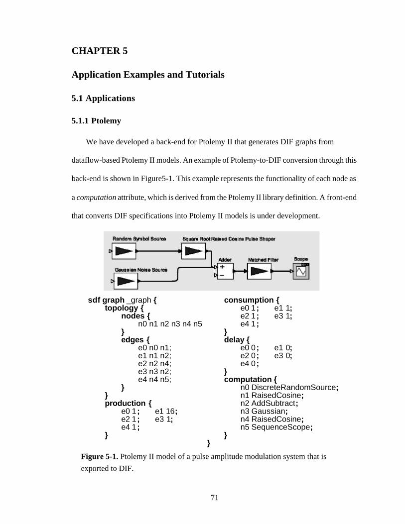
71
CHAPTER 5
Application Examples and Tutorials
5.1 Applications
5.1.1 Ptolemy
We have developed a back-end for Ptolemy II that generates DIF graphs from
dataflow-based Ptolemy II models. An example of Ptolemy-to-DIF conversion through this
back-end is shown in Figure5-1. This example represents the functionality of each node as
a computation attribute, which is derived from the Ptolemy II library definition. A front-end
that converts DIF specifications into Ptolemy II models is under development.
Figure 5-1. Ptolemy II model of a pulse amplitude modulation system that is exported to DIF.
sdf graph _graph {topology {
nodes {n0 n1 n2 n3 n4 n5
}edges {
e0 n0 n1;e1 n1 n2;e2 n2 n4;e3 n3 n2;e4 n4 n5;
}}production {
e0 1 ; e1 16;e2 1 ; e3 1;e4 1 ;
}
consumption {e0 1 ; e1 1;e2 1 ; e3 1;e4 1 ;
}delay {
e0 0 ; e1 0;e2 0 ; e3 0;e4 0 ;
}computation {
n0 DiscreteRandomSource;n1 RaisedCosine;n2 AddSubtract;n3 Gaussian;n4 RaisedCosine;n5 SequenceScope;
}}
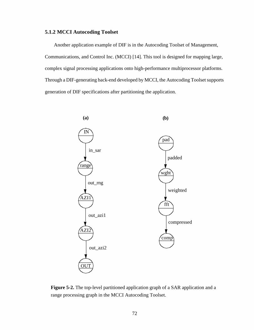
72
5.1.2 MCCI Autocoding Toolset
Another application example of DIF is in the Autocoding Toolset of Management,
Communications, and Control Inc. (MCCI) [14]. This tool is designed for mapping large,
complex signal processing applications onto high-performance multiprocessor platforms.
Through a DIF-generating back-end developed by MCCI, the Autocoding Toolset supports
generation of DIF specifications after partitioning the application.
OUT
AZI1
AZI2
range
in_sar
out_rng
out_azi1
out_azi2
fft
pad
wght
comp
padded
weighted
compressed
(a) (b)
IN
Figure 5-2. The top-level partitioned application graph of a SAR application and a range processing graph in the MCCI Autocoding Toolset.
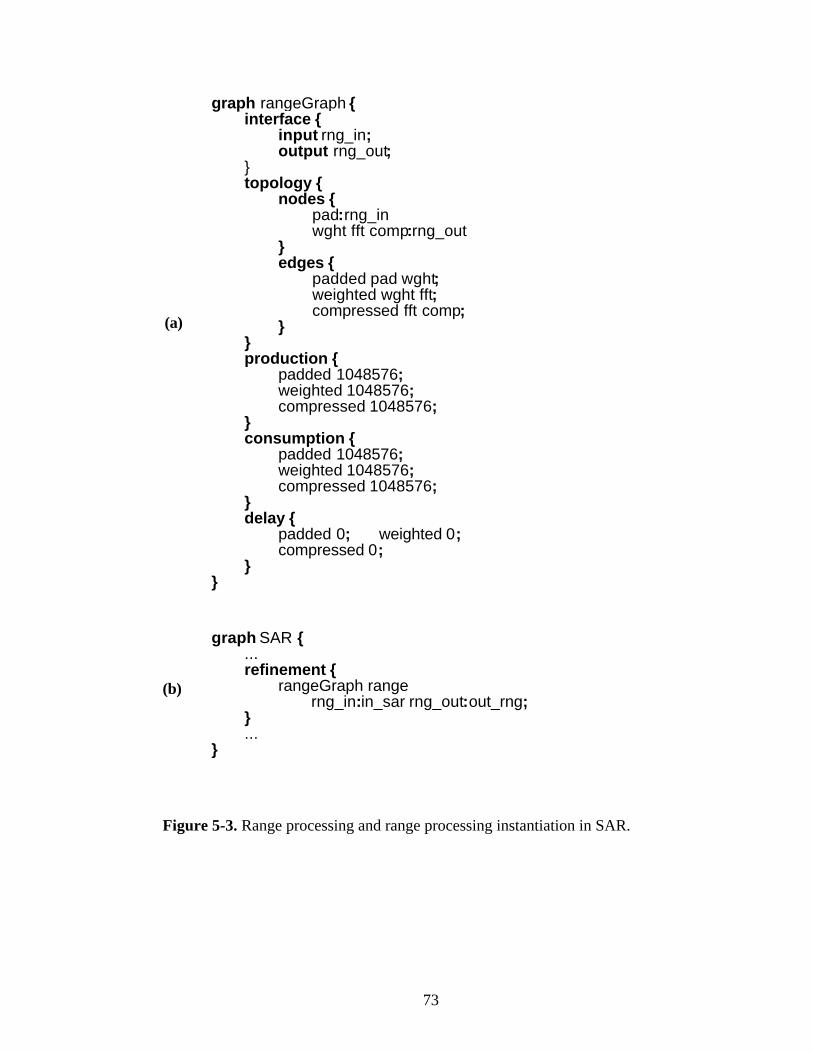
73
graph rangeGraph {interface {
input rng_in;output rng_out;
}topology {
nodes {pad:rng_in wght fft comp:rng_out
}edges {
padded pad wght;weighted wght fft;compressed fft comp;
}}production {
padded 1048576;weighted 1048576;compressed 1048576;
}consumption {
padded 1048576;weighted 1048576;compressed 1048576;
}delay {
padded 0; weighted 0;compressed 0;
}}
graph SAR {...refinement {
rangeGraph range rng_in:in_sar rng_out:out_rng;
}...
}
Figure 5-3. Range processing and range processing instantiation in SAR.
(a)
(b)
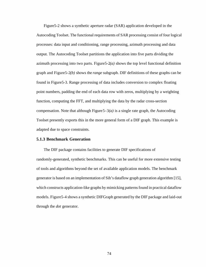
74
Figure5-2 shows a synthetic aperture radar (SAR) application developed in the
Autocoding Toolset. The functional requirements of SAR processing consist of four logical
processes: data input and conditioning, range processing, azimuth processing and data
output. The Autocoding Toolset partitions the application into five parts dividing the
azimuth processing into two parts. Figure5-2(a) shows the top level functional definition
graph and Figure5-2(b) shows the range subgraph. DIF definitions of these graphs can be
found in Figure5-3. Range processing of data includes conversion to complex floating
point numbers, padding the end of each data row with zeros, multiplying by a weighting
function, computing the FFT, and multiplying the data by the radar cross-section
compensation. Note that although Figure5-3(a) is a single rate graph, the Autocoding
Toolset presently exports this in the more general form of a DIF graph. This example is
adapted due to space constraints.
5.1.3 Benchmark Generation
The DIF package contains facilities to generate DIF specifications of
randomly-generated, synthetic benchmarks. This can be useful for more extensive testing
of tools and algorithms beyond the set of available application models. The benchmark
generator is based on an implementation of Sih’s dataflow graph generation algorithm [15],
which constructs application-like graphs by mimicking patterns found in practical dataflow
models. Figure5-4 shows a synthetic DIFGraph generated by the DIF package and laid-out
through the dot generator.
75
sdf graph _graph {topology {
nodes {n0 n1 n2 n3 n4 n5n6 n7 n8n9 n10 n11n12 n13 n14n15 n16 n17n18 n19 n20
}edges {
e0 n0 n1;e1 n0 n2;e2 n1 n3;e3 n2 n5;e4 n5 n4;...e31 n20 n13;
}}
production {e0 1;...e31 1;
}consumption {
e0 1;...e31 1;
}delay {
e0 0;...e31 0;
}}
Figure 5-4. A synthetic DIFGraph generated by the DIF package and dot generator output for the graph.
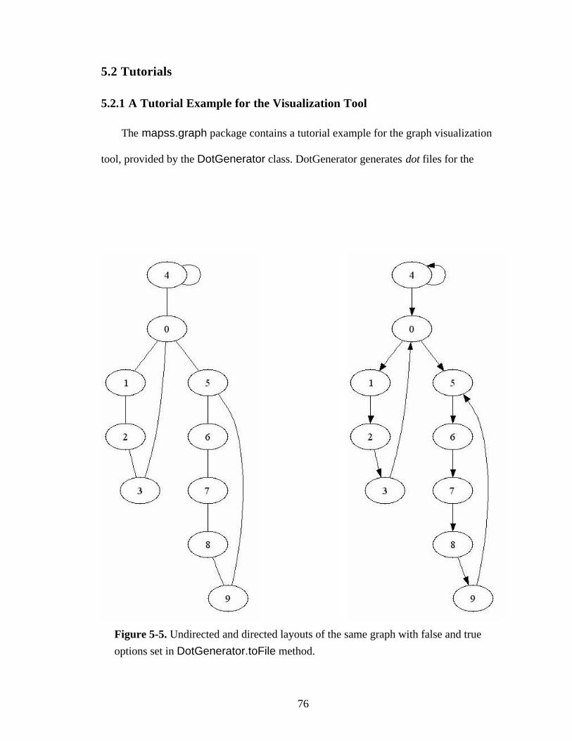
76
5.2 Tutorials
5.2.1 A Tutorial Example for the Visualization Tool
The mapss.graph package contains a tutorial example for the graph visualization
tool, provided by the DotGenerator class. DotGenerator generates dot files for the
Figure 5-5. Undirected and directed layouts of the same graph with false and true options set in DotGenerator.toFile method.
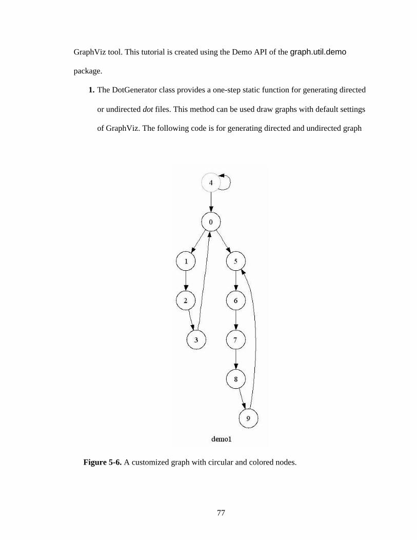
77
GraphViz tool. This tutorial is created using the Demo API of the graph.util.demo
package.
1. The DotGenerator class provides a one-step static function for generating directed
or undirected dot files. This method can be used draw graphs with default settings
of GraphViz. The following code is for generating directed and undirected graph
Figure 5-6. A customized graph with circular and colored nodes.
78
visualization files for a hypothetical Graph object named graph0. The last
parameter should be set to true for a directed output.
DotGenerator.toFile(graph0, fileName, true or false);
2. DotGenerator can be configured for a customized look. For changing default
options of the tool, a DotGenerator object is required to be created instead of
using the static function. The following is the code that generates the look in
Figure5-6.
// Create the DotGenerator object.DotGenerator dot = new DotGenerator(myGraph);
// Add some attributes to the graph to make it look nicer.// Note that attributes that belong to the graph (not specific// to an edge or a node) should be added with addLine method.dot.setGraphName("demo1");dot.addLine("node[shape = circle];");dot.addLine("center = true;");
// Add an attribute to a node in the graph.dot.setAttribute(node4, "color", "red");
// Set the graph as directed.dot.setAsDirected(true);
// Call toFile function to create the file.dot.toFile(path + "demo1");
3. GraphViz can also cluster graph nodes. Invisible nodes can be used to fine-tune the
alignment of nodes in clusters. In the graph of Figure5-7, invisible edges connect
79
nodes 2 and 5 to an invisible node at the bottom of the figure, which helps
GraphViz to place cluster nodes in two rows.
// Add a dummy node and two dummy edges to the graph for alignment// purposes.myGraph2.addNode(node7);Edge edge2_7 = myGraph2.addEdge(node2, node7);Edge edge5_7 = myGraph2.addEdge(node5, node7);
// Cluster the nodes after creating the DotGenerator object.DotGenerator dot2 = new DotGenerator(myGraph2);Collection cluster1 =Arrays.asList(new Node[] {node0, node1, node2});Collection cluster2 =Arrays.asList(new Node[] {node3, node4, node5});dot2.setCluster(cluster1);dot2.setCluster(cluster2);
// Set some attributes for a nice look.dot2.setAttribute(cluster1, "label = \"cluster1\"");dot2.setAttribute(cluster1, "color = blue");dot2.setAttribute(cluster2, "label = \"cluster2\"");dot2.setAttribute(cluster2, "color = red");
// Use this part of the graph for alignment purposes so set it// invisible.dot2.setAttribute(node7, "style", "\"invis\"");dot2.setAttribute(edge2_7, "style", "\"invis\"");dot2.setAttribute(edge5_7, "style", "\"invis\"");
// Set as directed.dot2.setAsDirected(true);
// Call toFile function to create the file.dot2.toFile(path + "clusterExample");
5.2.2 Tutorial Examples for the Hierarchy Mechanism
The mapss.graph.hierarchy package contains a tutorial example for the hierarchy
mechanism. This tutorial is created using the Demo API of the graph.util.demo package.
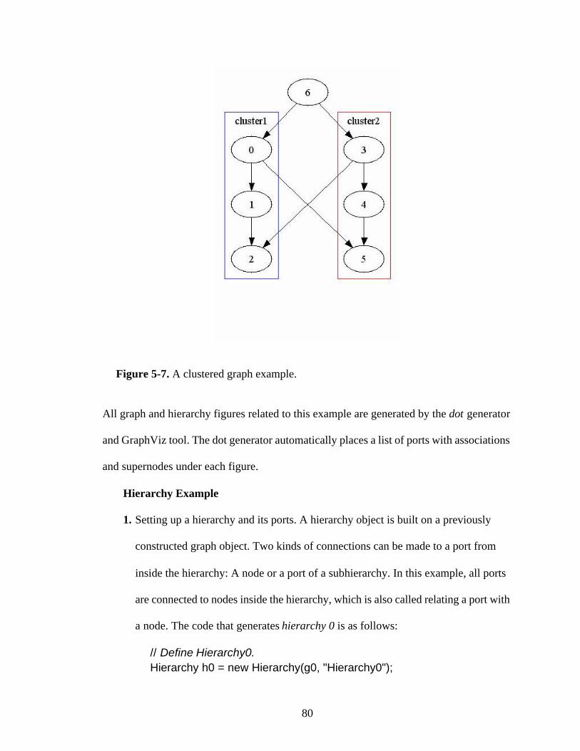
80
All graph and hierarchy figures related to this example are generated by the dot generator
and GraphViz tool. The dot generator automatically places a list of ports with associations
and supernodes under each figure.
Hierarchy Example
1. Setting up a hierarchy and its ports. A hierarchy object is built on a previously
constructed graph object. Two kinds of connections can be made to a port from
inside the hierarchy: A node or a port of a subhierarchy. In this example, all ports
are connected to nodes inside the hierarchy, which is also called relating a port with
a node. The code that generates hierarchy 0 is as follows:
// Define Hierarchy0.Hierarchy h0 = new Hierarchy(g0, "Hierarchy0");
Figure 5-7. A clustered graph example.
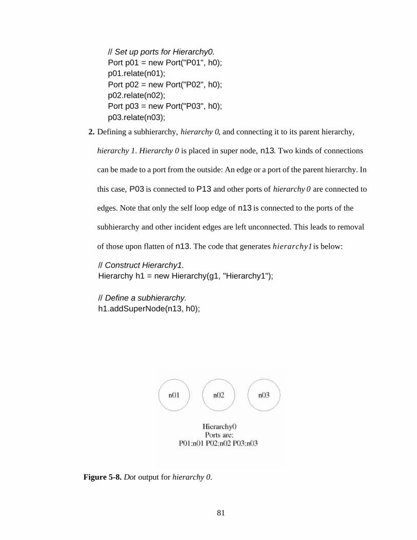
81
// Set up ports for Hierarchy0.Port p01 = new Port("P01", h0);p01.relate(n01);Port p02 = new Port("P02", h0);p02.relate(n02);Port p03 = new Port("P03", h0);p03.relate(n03);
2. Defining a subhierarchy, hierarchy 0, and connecting it to its parent hierarchy,
hierarchy 1. Hierarchy 0 is placed in super node, n13. Two kinds of connections
can be made to a port from the outside: An edge or a port of the parent hierarchy. In
this case, P03 is connected to P13 and other ports of hierarchy 0 are connected to
edges. Note that only the self loop edge of n13 is connected to the ports of the
subhierarchy and other incident edges are left unconnected. This leads to removal
of those upon flatten of n13. The code that generates hierarchy1 is below:
// Construct Hierarchy1.Hierarchy h1 = new Hierarchy(g1, "Hierarchy1");
// Define a subhierarchy.h1.addSuperNode(n13, h0);
Figure 5-8. Dot output for hierarchy 0.
82
// Make connections from outside (Hierarchy1) to the subhierarchy// (Hierarchy0).p01.connect(e15);p02.connect(e15);
// Set up ports for Hierarchy1 and connect them with nodes// from the inside.Port p11 = new Port("P11", h1);p11.relate(n11);Port p12 = new Port("P12", h1);p12.relate(n14);
// The following port is connected to a port from a subhierarchy instead// of a node.Port p13 = new Port("P13", h1);p13.relate(p03);
3. This time hierarchy 1 is defined as a subhierarchy of hierarchy 2 in the code
example below.
// Construct Hierarchy2Hierarchy h2 = new Hierarchy(g2, "Hierarchy2");
// Define a subhierarchy.h2.addSuperNode(n23, h1);
// Make connections from outside (Hierarchy2) to the subhierarchy// (Hierarchy1).p11.connect(e22);p12.connect(e23);
// Set up ports for Hierarchy2 and connect them with nodes// from the inside.Port p21 = new Port("P21", h2);p21.relate(n21);Port p22 = new Port("P22", h2);p22.relate(n22);
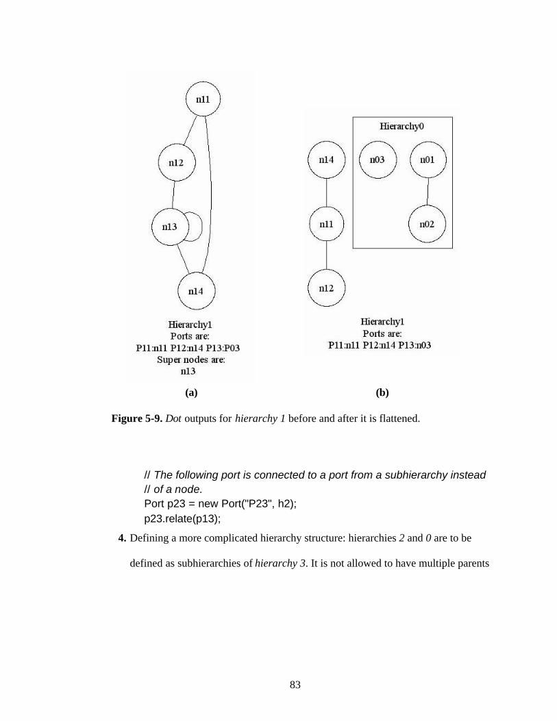
83
// The following port is connected to a port from a subhierarchy instead// of a node.Port p23 = new Port("P23", h2);p23.relate(p13);
4. Defining a more complicated hierarchy structure: hierarchies 2 and 0 are to be
defined as subhierarchies of hierarchy 3. It is not allowed to have multiple parents
Figure 5-9. Dot outputs for hierarchy 1 before and after it is flattened.
(a) (b)
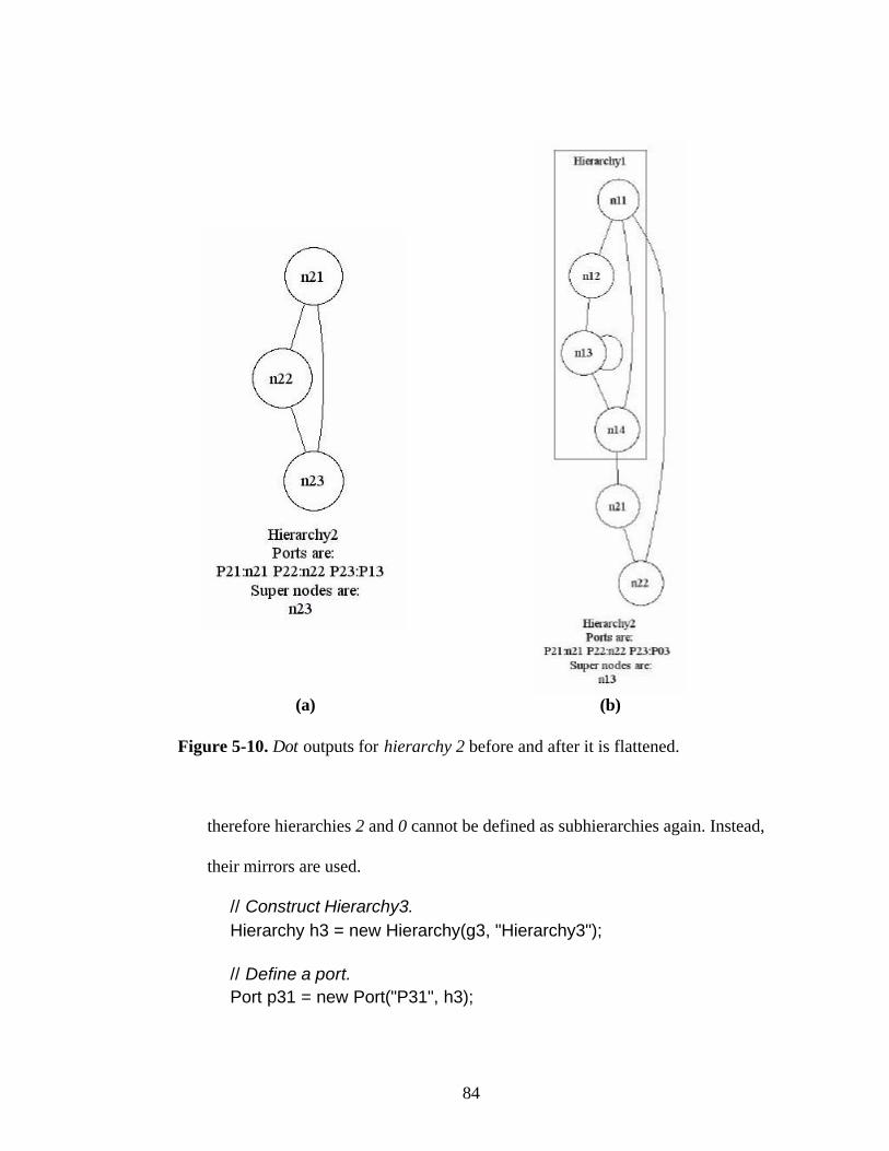
84
therefore hierarchies 2 and 0 cannot be defined as subhierarchies again. Instead,
their mirrors are used.
// Construct Hierarchy3.Hierarchy h3 = new Hierarchy(g3, "Hierarchy3");
// Define a port.Port p31 = new Port("P31", h3);
Figure 5-10. Dot outputs for hierarchy 2 before and after it is flattened.
(a) (b)
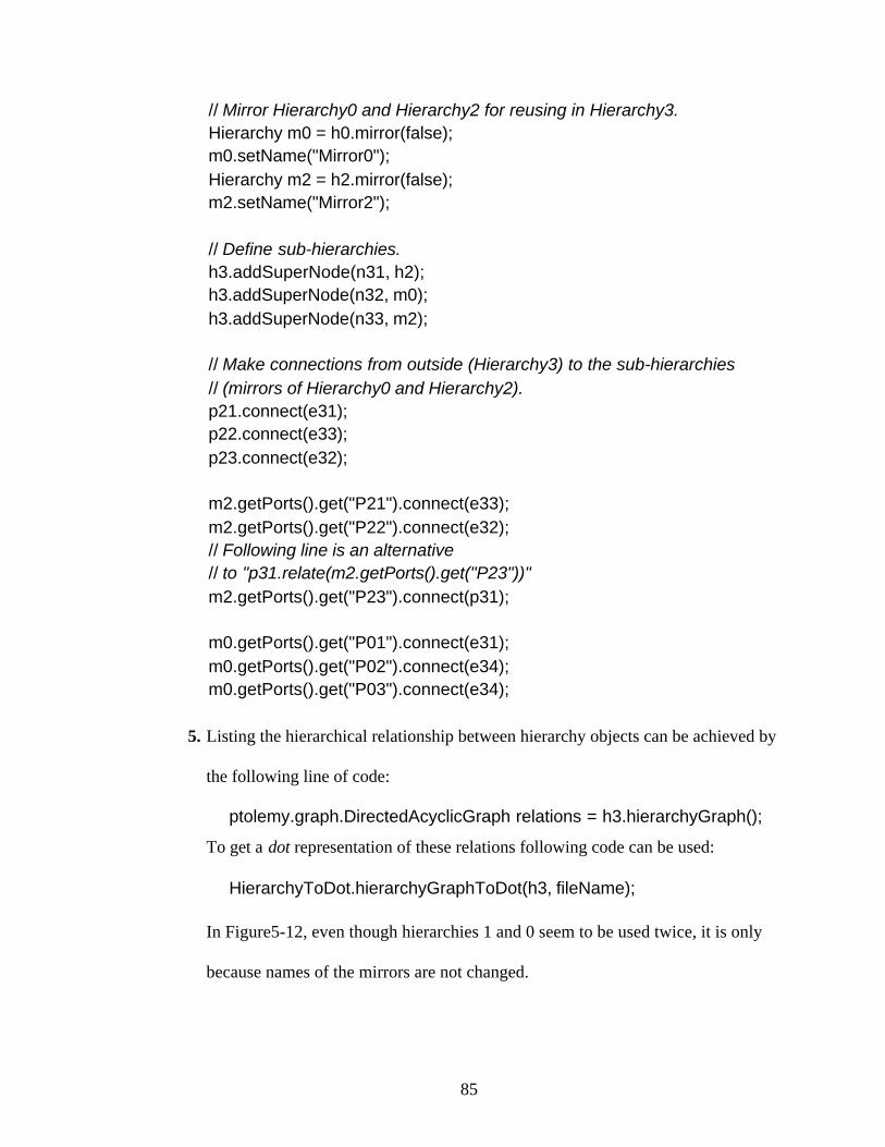
85
// Mirror Hierarchy0 and Hierarchy2 for reusing in Hierarchy3.Hierarchy m0 = h0.mirror(false);m0.setName("Mirror0");Hierarchy m2 = h2.mirror(false);m2.setName("Mirror2");
// Define sub-hierarchies.h3.addSuperNode(n31, h2);h3.addSuperNode(n32, m0);h3.addSuperNode(n33, m2);
// Make connections from outside (Hierarchy3) to the sub-hierarchies// (mirrors of Hierarchy0 and Hierarchy2).p21.connect(e31);p22.connect(e33);p23.connect(e32);
m2.getPorts().get("P21").connect(e33);m2.getPorts().get("P22").connect(e32);// Following line is an alternative// to "p31.relate(m2.getPorts().get("P23"))"m2.getPorts().get("P23").connect(p31);
m0.getPorts().get("P01").connect(e31);m0.getPorts().get("P02").connect(e34);m0.getPorts().get("P03").connect(e34);
5. Listing the hierarchical relationship between hierarchy objects can be achieved by
the following line of code:
ptolemy.graph.DirectedAcyclicGraph relations = h3.hierarchyGraph();
To get a dot representation of these relations following code can be used:
HierarchyToDot.hierarchyGraphToDot(h3, fileName);
In Figure5-12, even though hierarchies 1 and 0 seem to be used twice, it is only
because names of the mirrors are not changed.
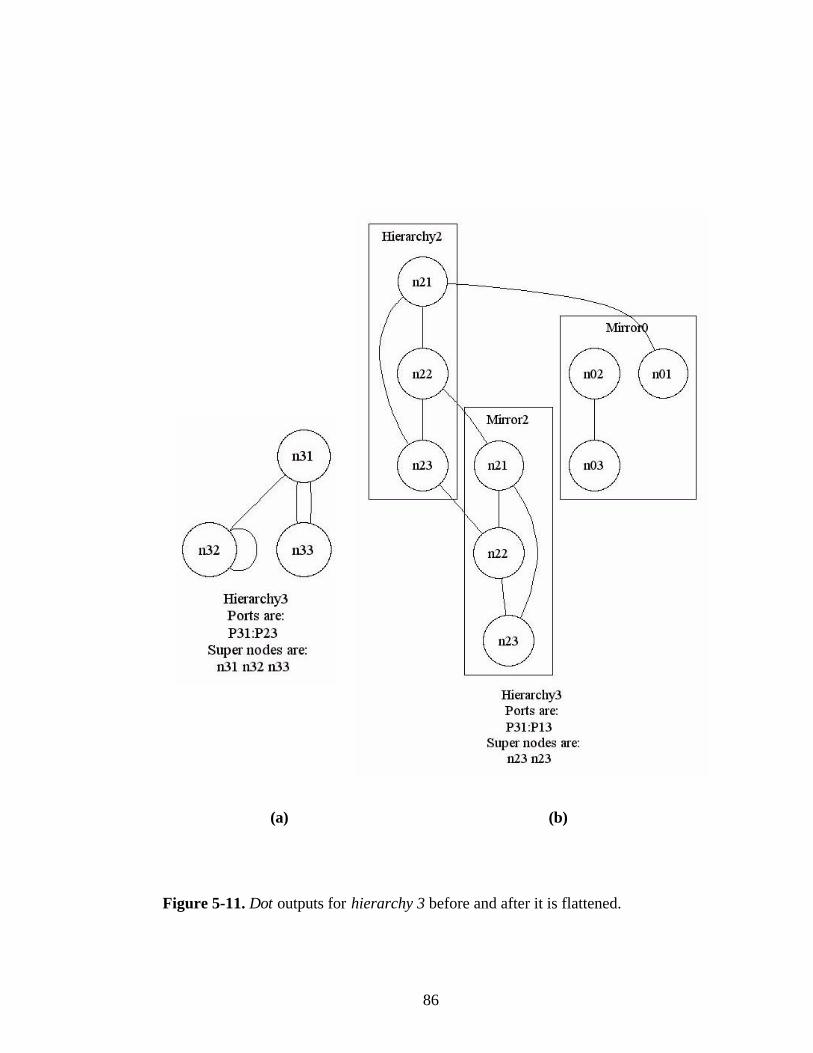
86
Figure 5-11. Dot outputs for hierarchy 3 before and after it is flattened.
(a) (b)
87
Directed Hierarchy Example
1. Directed hierarchies are defined in the same way as hierarchies. The difference is
the additional direction parameter in the Port constructor and also the visualization
tool is configured to show edge directions as well. The code that defines a directed
port is
Port directedPort = new Port("Name", hierarchy, direction);
Figure 5-12. Dot outputs for hierarchy tree graph.
88
where the values that the direction parameter can take are Port.IN are Port.OUT.
An undirected port can be used as a bidirectional port. This example uses the same
graphs as the previous example.
2. Directed hierarchies require extra attention to maintain consistency between
connections and port directions. Trying to connect an incoming edge to an output
port or vice versa will result in an error. Likewise, if ports are connected together,
their directions should be the same, with the exception of undirected ports. A
bidirectional (or undirected) port can be connected to an edge or port regardless of
the direction, however it cannot be related to a directed port. One example of port
direction matching is P01 of hierarchy 0 (Figure 5-13(a)). Despite the fact that P01
is an OUT port in the original hierarchy, the same port in the mirror of hierarchy 0
is connected to an incoming edge of Hierarchy 3. This is only possible by manually
removing that port and defining another port with IN or no direction
(Figure5-13(b)):
// Remove Port 01 in the mirror.Port oldPort = mirror0.getPorts().get("P01");Node relatedNode = oldPort.getNode();oldPort.dispose();
// Replace the old port with a new port with no direction.(new Port("P01", mirror0)).relate(relatedNode);
// Connect the port to the incoming edge.mirror0.getPorts().get("P01").connect(e31);
Finally, hierarchy 3 is deep-flattened, merging all levels of the hierarchy in a single
graph. Note that some of the node labels are duplicated. This is because same node
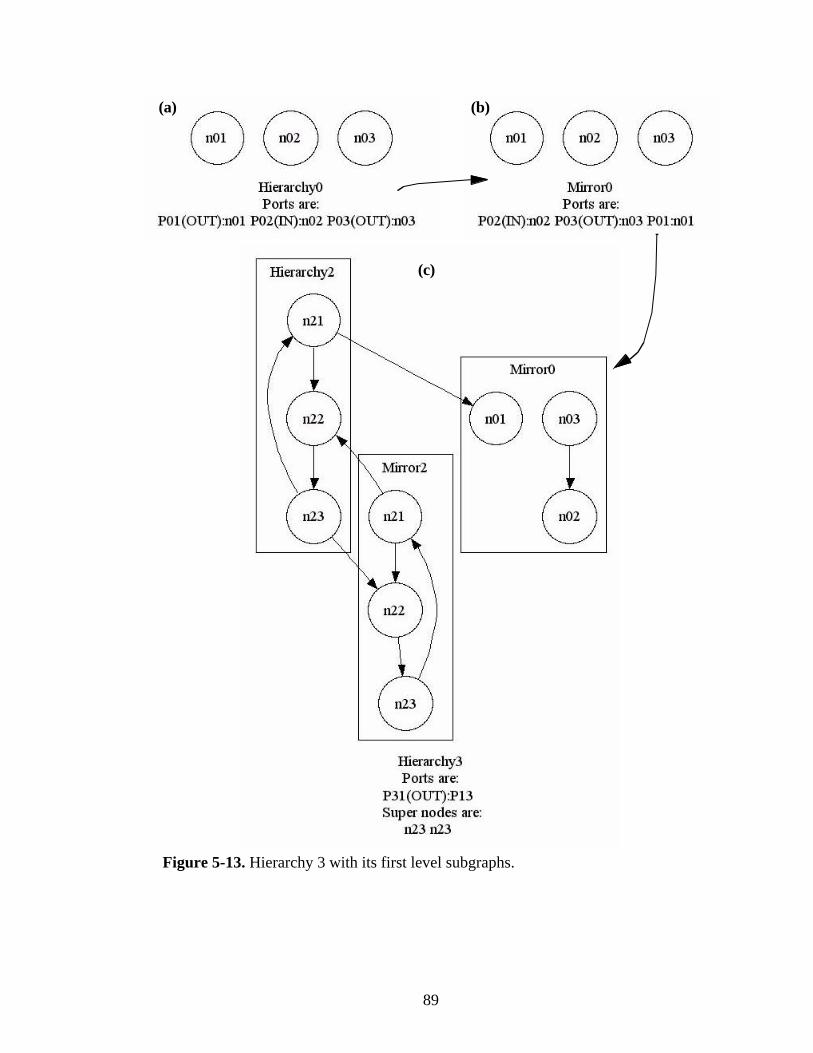
89
Figure 5-13. Hierarchy 3 with its first level subgraphs.
(a) (b)
(c)
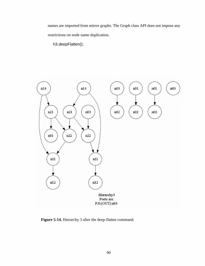
90
names are imported from mirror graphs. The Graph class API does not impose any
restrictions on node name duplication.
h3.deepFlatten();
Figure 5-14. Hierarchy 3 after the deep-flatten command.
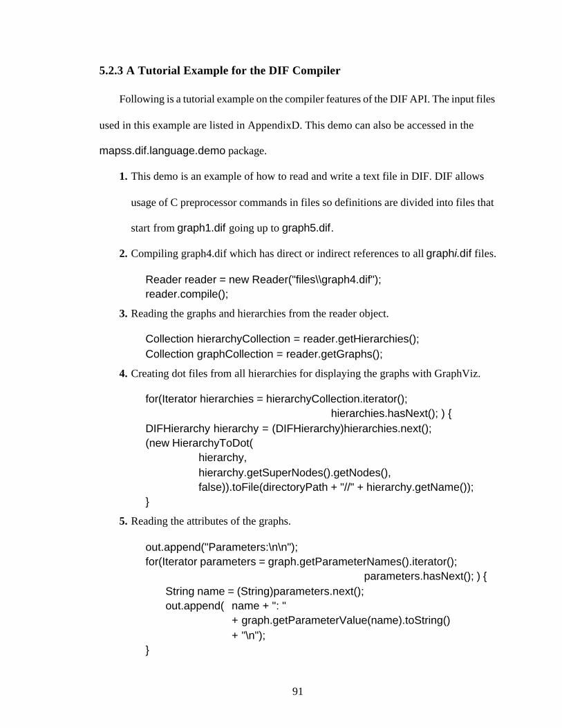
91
5.2.3 A Tutorial Example for the DIF Compiler
Following is a tutorial example on the compiler features of the DIF API. The input files
used in this example are listed in AppendixD. This demo can also be accessed in the
mapss.dif.language.demo package.
1. This demo is an example of how to read and write a text file in DIF. DIF allows
usage of C preprocessor commands in files so definitions are divided into files that
start from graph1.dif going up to graph5.dif.
2. Compiling graph4.dif which has direct or indirect references to all graphi.dif files.
Reader reader = new Reader("files\\graph4.dif");reader.compile();
3. Reading the graphs and hierarchies from the reader object.
Collection hierarchyCollection = reader.getHierarchies();Collection graphCollection = reader.getGraphs();
4. Creating dot files from all hierarchies for displaying the graphs with GraphViz.
for(Iterator hierarchies = hierarchyCollection.iterator();hierarchies.hasNext(); ) {
DIFHierarchy hierarchy = (DIFHierarchy)hierarchies.next();(new HierarchyToDot(
hierarchy,hierarchy.getSuperNodes().getNodes(),false)).toFile(directoryPath + "//" + hierarchy.getName());
}
5. Reading the attributes of the graphs.
out.append("Parameters:\n\n");for(Iterator parameters = graph.getParameterNames().iterator();
parameters.hasNext(); ) {String name = (String)parameters.next();out.append( name + ": "
+ graph.getParameterValue(name).toString()+ "\n");
}
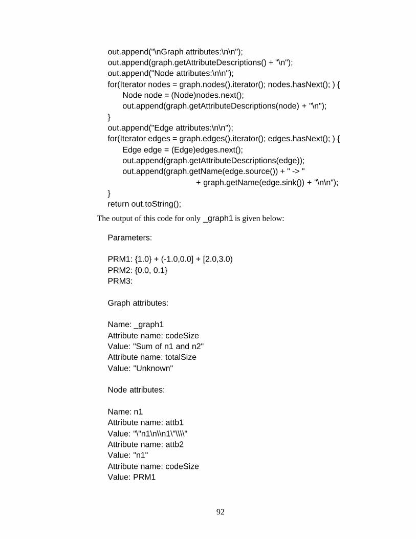
92
out.append("\nGraph attributes:\n\n");out.append(graph.getAttributeDescriptions() + "\n");out.append("Node attributes:\n\n");for(Iterator nodes = graph.nodes().iterator(); nodes.hasNext(); ) {
Node node = (Node)nodes.next();out.append(graph.getAttributeDescriptions(node) + "\n");
}out.append("Edge attributes:\n\n");for(Iterator edges = graph.edges().iterator(); edges.hasNext(); ) {
Edge edge = (Edge)edges.next();out.append(graph.getAttributeDescriptions(edge));out.append(graph.getName(edge.source()) + " -> "
+ graph.getName(edge.sink()) + "\n\n");}return out.toString();
The output of this code for only _graph1 is given below:
Parameters:
PRM1: {1.0} + (-1.0,0.0] + [2.0,3.0)PRM2: {0.0, 0.1}PRM3:
Graph attributes:
Name: _graph1Attribute name: codeSizeValue: "Sum of n1 and n2"Attribute name: totalSizeValue: "Unknown"
Node attributes:
Name: n1Attribute name: attb1Value: "\"n1\n\\n1\"\\\\"Attribute name: attb2Value: "n1"Attribute name: codeSizeValue: PRM1
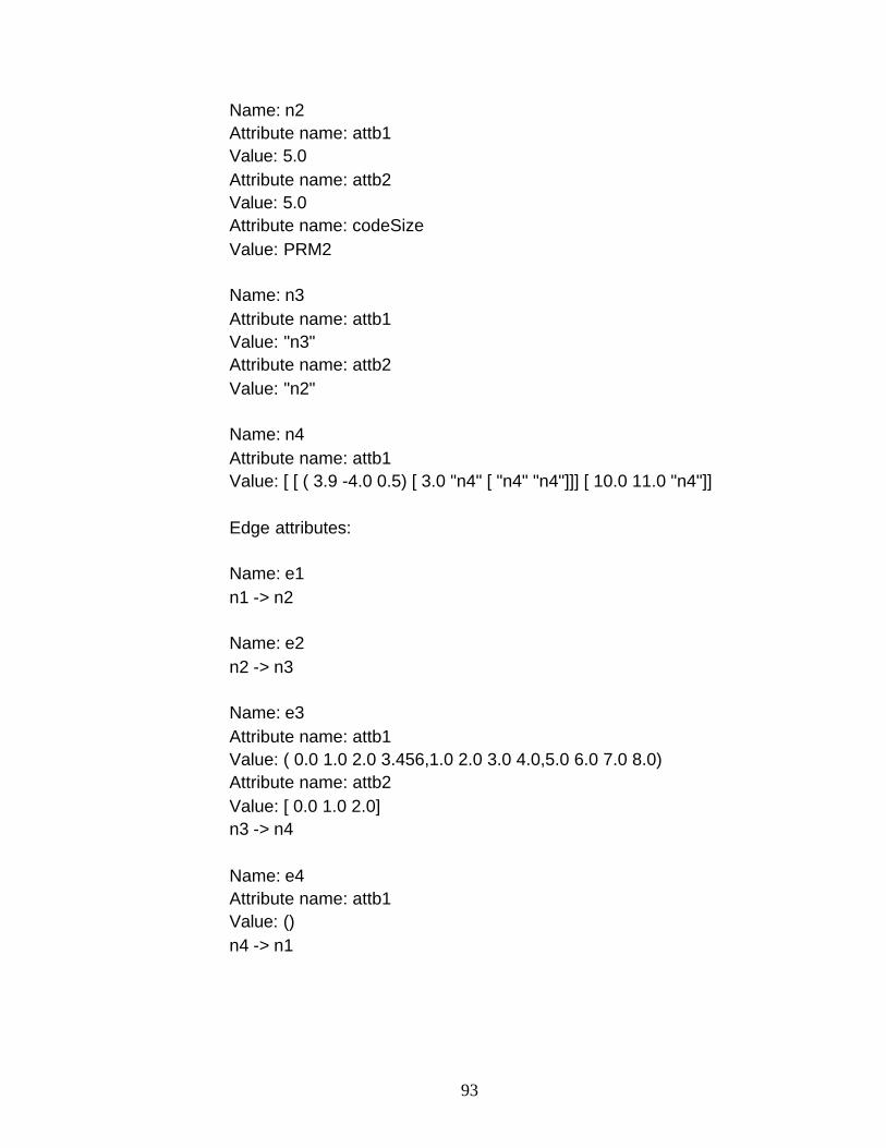
93
Name: n2Attribute name: attb1Value: 5.0Attribute name: attb2Value: 5.0Attribute name: codeSizeValue: PRM2
Name: n3Attribute name: attb1Value: "n3"Attribute name: attb2Value: "n2"
Name: n4Attribute name: attb1Value: [ [ ( 3.9 -4.0 0.5) [ 3.0 "n4" [ "n4" "n4"]]] [ 10.0 11.0 "n4"]]
Edge attributes:
Name: e1n1 -> n2
Name: e2n2 -> n3
Name: e3Attribute name: attb1Value: ( 0.0 1.0 2.0 3.456,1.0 2.0 3.0 4.0,5.0 6.0 7.0 8.0)Attribute name: attb2Value: [ 0.0 1.0 2.0]n3 -> n4
Name: e4Attribute name: attb1Value: ()n4 -> n1
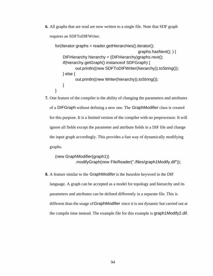
94
6. All graphs that are read are now written to a single file. Note that SDF graph
requires an SDFToDIFWriter.
for(Iterator graphs = reader.getHierarchies().iterator();graphs.hasNext(); ) {
DIFHierarchy hierarchy = (DIFHierarchy)graphs.next();if(hierarchy.getGraph() instanceof SDFGraph) {
out.println((new SDFToDIFWriter(hierarchy)).toString());} else {
out.println((new Writer(hierarchy)).toString());}
}
7. One feature of the compiler is the ability of changing the parameters and attributes
of a DIFGraph without defining a new one. The GraphModifier class is created
for this purpose. It is a limited version of the compiler with no preprocessor. It will
ignore all fields except the parameter and attribute fields in a DIF file and change
the input graph accordingly. This provides a fast way of dynamically modifying
graphs.
(new GraphModifier(graph1)).modifyGraph(new FileReader("./files/graph1Modify.dif"));
8. A feature similar to the GraphModifer is the basedon keyword in the DIF
language. A graph can be accepted as a model for topology and hierarchy and its
parameters and attributes can be defined differently in a separate file. This is
different than the usage of GraphModifier since it is not dynamic but carried out at
the compile time instead. The example file for this example is graph1Modify2.dif.
95
CHAPTER 6
Conclusion
This thesis has presented the first version (version 0.1) of dataflow interchange format
(DIF), a textual language for writing coarse-grain, dataflow-based models of DSP
applications, and for communicating such models between DSP design tools. The
objectives of DIF are to accommodate a variety of dataflow-related modeling constructs,
and to facilitate experimentation with and technology transfer involving such constructs.
The DIF language is actively being extended, including the set of supported dataflow
modeling semantics, language features and repository of intermediate representations and
algorithms. Many of these extensions will be contained in the forthcoming next version,
DIF 0.2. Support for DIF has already been incorporated in an individual dataflow-based
design tool - the MCCI Autocoding Toolset [14].
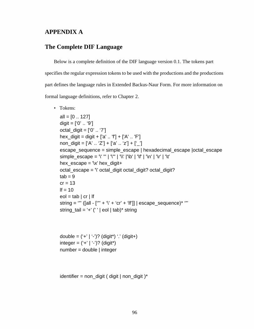
96
APPENDIX A
The Complete DIF Language
Below is a complete definition of the DIF language version 0.1. The tokens part
specifies the regular expression tokens to be used with the productions and the productions
part defines the language rules in Extended Backus-Naur Form. For more information on
formal language definitions, refer to Chapter 2.
• Tokens:
all = [0 .. 127]digit = [‘0’ .. ‘9’]octal_digit = [‘0’ .. ‘7’]hex_digit = digit + ['a' .. 'f'] + ['A' .. 'F']non_digit = [‘A’ .. ‘Z’] + [‘a’ .. ‘z’] + [‘_’]escape_sequence = simple_escape | hexadecimal_escape |octal_escapesimple_escape = '\' ''' | '\"' | '\\' |'\b' | '\f' | '\n' | '\r' | '\t’hex_escape = '\x' hex_digit+octal_escape = '\' octal_digit octal_digit? octal_digit?tab = 9cr = 13lf = 10eol = tab | cr | lfstring = ‘”’ ([all - [‘”’ + ‘\’ + ‘cr’ + ‘lf’]] | escape_sequence)* ‘”’string_tail = '+' (' ' | eol | tab)* string
double = (‘+’ | ‘-’)? (digit*) ‘.’ (digit+)integer = (‘+’ | ‘-’)? (digit*)number = double | integer
identifier = non_digit ( digit | non_digit )*
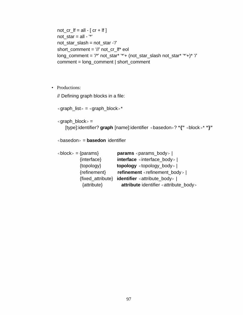
97
not_cr_lf = all - [ cr + lf ]not_star = all - '*'not_star_slash = not_star -'/'short_comment = '//' not_cr_lf* eollong_comment = '/*' not_star* '*'+ (not_star_slash not_star* '*'+)* '/'comment = long_comment | short_comment
• Productions:
// Defining graph blocks in a file:
<graph_list> = <graph_block>*
<graph_block> =[type]:identifier? graph [name]:identifier <basedon>? “{” <block>* “}”
<basedon> = basedon identifier
<block> = {params} params <params_body> |{interface} interface <interface_body> |{topology} topology <topology_body> |{refinement} refinement <refinement_body> |{fixed_attribute} identifier <attribute_body> |{attribute} attribute identifier <attribute_body>
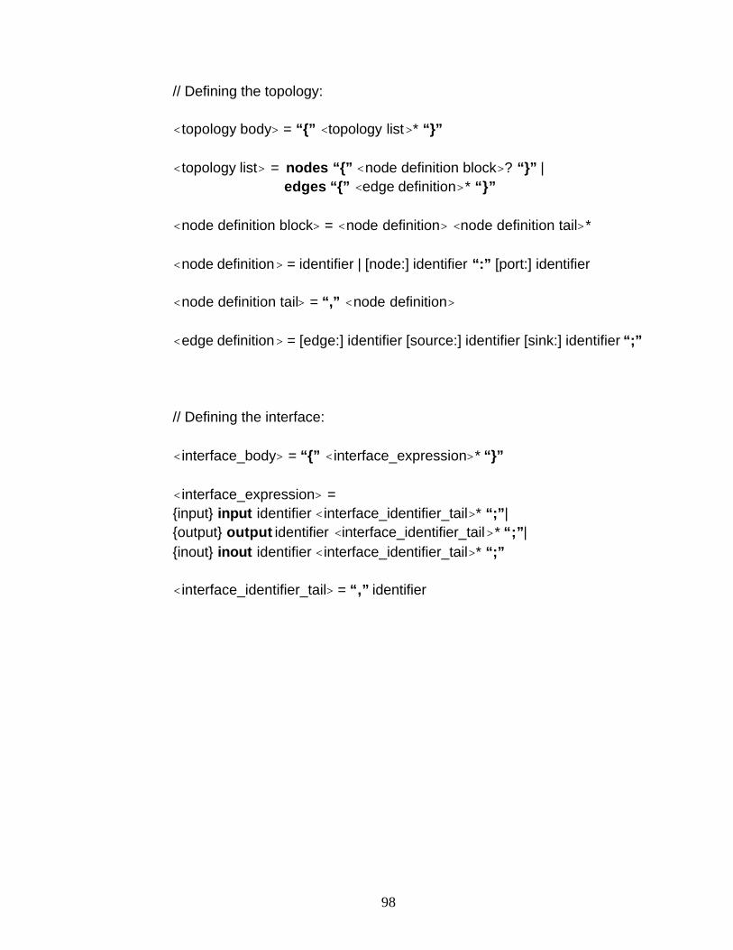
98
// Defining the topology:
<topology body> = “{” <topology list>* “}”
<topology list> = nodes “{” <node definition block>? “}” |edges “{” <edge definition>* “}”
<node definition block> = <node definition> <node definition tail>*
<node definition> = identifier | [node:] identifier “:” [port:] identifier
<node definition tail> = “,” <node definition>
<edge definition> = [edge:] identifier [source:] identifier [sink:] identifier “;”
// Defining the interface:
<interface_body> = “{” <interface_expression>* “}”
<interface_expression> ={input} input identifier <interface_identifier_tail>* “;”|{output} output identifier <interface_identifier_tail>* “;”|{inout} inout identifier <interface_identifier_tail>* “;”
<interface_identifier_tail> = “,” identifier
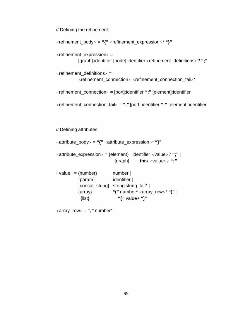
99
// Defining the refinement:
<refinement_body> = “{” <refinement_expression>* “}”
<refinement_expression> =[graph]:identifier [node]:identifier <refinement_definitions>? “;”
<refinement_definitions> =<refinement_connection> <refinement_connection_tail>*
<refinement_connection> = [port]:identifier “:” [element]:identifier
<refinement_connection_tail> = “,” [port]:identifier “:” [element]:identifier
// Defining attributes:
<attribute_body> = “{” <attribute_expression>* “}”
<attribute_expression> = {element} identifier <value>? “;” |{graph} this <value>? “;”
<value> = {number} number |{param} identifier |{concat_string} string string_tail* |{array} “(” number* <array_row>* “)” |{list} “[” value+ “]”
<array_row> = “,” number*
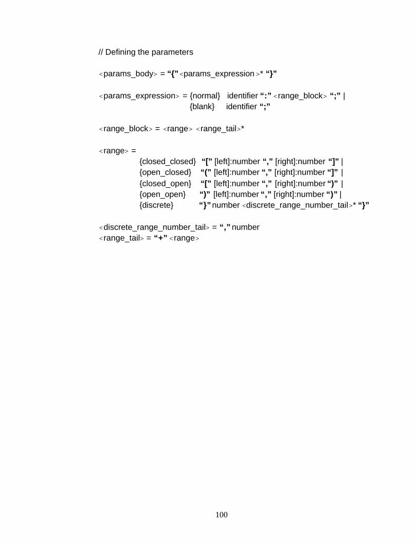
100
// Defining the parameters
<params_body> = “{”<params_expression>* “}”
<params_expression> = {normal} identifier “:” <range_block> “;” |{blank} identifier “;”
<range_block> = <range> <range_tail>*
<range> ={closed_closed} “[” [left]:number “,” [right]:number “]” |{open_closed} “(” [left]:number “,” [right]:number “]” |{closed_open} “[” [left]:number “,” [right]:number “)” |{open_open} “)” [left]:number “,” [right]:number “)” |{discrete} “}” number <discrete_range_number_tail>* “}”
<discrete_range_number_tail> = “,” number<range_tail> = “+” <range>
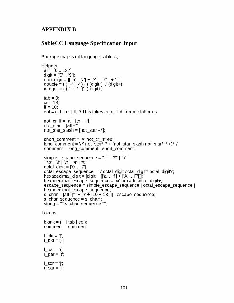
101
APPENDIX B
SableCC Language Specification Input
Package mapss.dif.language.sablecc;
Helpers all = [0 .. 127]; digit = ['0' .. '9']; non_digit = [[['a' .. 'z'] + ['A' .. 'Z']] + '_']; double = ( ( '+' | '-' )? ) (digit*) '.' (digit+); integer = ( ( '+' | '-' )? ) digit+;
tab = 9; cr = 13; lf = 10; eol = cr lf | cr | lf; // This takes care of different platforms
not_cr_lf = [all -[cr + lf]]; not_star = [all -'*']; not_star_slash = [not_star -'/'];
short_comment = '//' not_cr_lf* eol; long_comment = '/*' not_star* '*'+ (not_star_slash not_star* '*'+)* '/'; comment = long_comment | short_comment;
simple_escape_sequence = '\' ''' | '\"' | '\\' | '\b' | '\f' | '\n' | '\r' | '\t'; octal_digit = ['0' .. '7']; octal_escape_sequence = '\' octal_digit octal_digit? octal_digit?; hexadecimal_digit = [digit + [['a' .. 'f'] + ['A' .. 'F']]]; hexadecimal_escape_sequence = '\x' hexadecimal_digit+; escape_sequence = simple_escape_sequence | octal_escape_sequence | hexadecimal_escape_sequence; s_char = [all -['"' + ['\' + [10 + 13]]]] | escape_sequence; s_char_sequence = s_char*; string = '"' s_char_sequence '"';
Tokens
blank = (' ' | tab | eol); comment = comment;
l_bkt = '{'; r_bkt = '}';
l_par = '('; r_par = ')';
l_sqr = '['; r_sqr = ']';
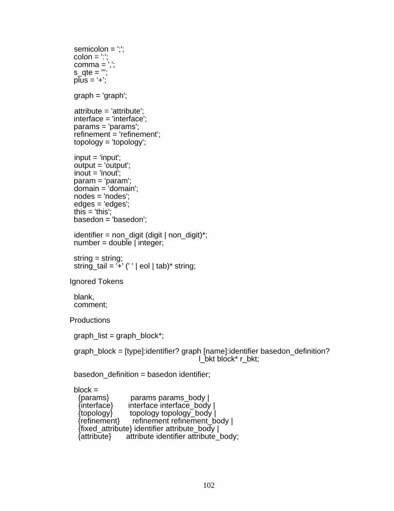
102
semicolon = ';'; colon = ':'; comma = ','; s_qte = '''; plus = '+';
graph = 'graph';
attribute = 'attribute'; interface = 'interface'; params = 'params'; refinement = 'refinement'; topology = 'topology';
input = 'input'; output = 'output'; inout = 'inout'; param = 'param'; domain = 'domain'; nodes = 'nodes'; edges = 'edges'; this = 'this'; basedon = 'basedon';
identifier = non_digit (digit | non_digit)*; number = double | integer;
string = string; string_tail = '+' (' ' | eol | tab)* string;
Ignored Tokens
blank, comment;
Productions
graph_list = graph_block*;
graph_block = [type]:identifier? graph [name]:identifier basedon_definition? l_bkt block* r_bkt;
basedon_definition = basedon identifier;
block = {params} params params_body | {interface} interface interface_body | {topology} topology topology_body | {refinement} refinement refinement_body | {fixed_attribute} identifier attribute_body | {attribute} attribute identifier attribute_body;
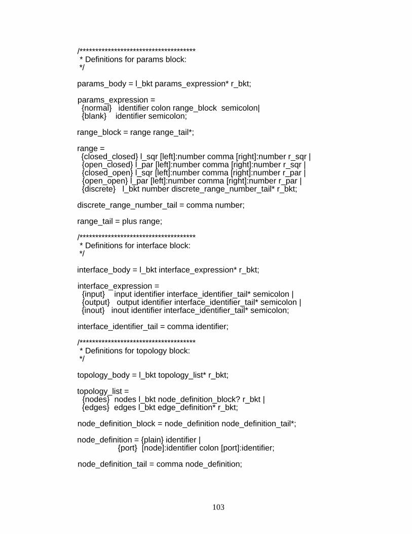
103
/************************************* * Definitions for params block: */
params_body = l_bkt params_expression* r_bkt;
params_expression = {normal} identifier colon range_block semicolon| {blank} identifier semicolon;
range_block = range range_tail*;
range = {closed_closed} l_sqr [left]:number comma [right]:number r_sqr | {open_closed} l_par [left]:number comma [right]:number r_sqr | {closed_open} l_sqr [left]:number comma [right]:number r_par | {open_open} l_par [left]:number comma [right]:number r_par | {discrete} l_bkt number discrete_range_number_tail* r_bkt;
discrete_range_number_tail = comma number;
range_tail = plus range;
/************************************* * Definitions for interface block: */
interface_body = l_bkt interface_expression* r_bkt;
interface_expression = {input} input identifier interface_identifier_tail* semicolon | {output} output identifier interface_identifier_tail* semicolon | {inout} inout identifier interface_identifier_tail* semicolon;
interface_identifier_tail = comma identifier;
/************************************* * Definitions for topology block: */
topology_body = l_bkt topology_list* r_bkt;
topology_list = {nodes} nodes l_bkt node_definition_block? r_bkt | {edges} edges l_bkt edge_definition* r_bkt;
node_definition_block = node_definition node_definition_tail*;
node_definition = {plain} identifier | {port} [node]:identifier colon [port]:identifier;
node_definition_tail = comma node_definition;
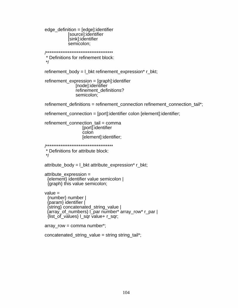
104
edge_definition = [edge]:identifier [source]:identifier [sink]:identifier semicolon;
/************************************* * Definitions for refinement block: */
refinement_body = l_bkt refinement_expression* r_bkt;
refinement_expression = [graph]:identifier [node]:identifier refinement_definitions? semicolon;
refinement_definitions = refinement_connection refinement_connection_tail*;
refinement_connection = [port]:identifier colon [element]:identifier;
refinement_connection_tail = comma [port]:identifier colon [element]:identifier;
/************************************* * Definitions for attribute block: */
attribute_body = l_bkt attribute_expression* r_bkt;
attribute_expression = {element} identifier value semicolon | {graph} this value semicolon;
value = {number} number | {param} identifier | {string} concatenated_string_value | {array_of_numbers} l_par number* array_row* r_par | {list_of_values} l_sqr value+ r_sqr;
array_row = comma number*;
concatenated_string_value = string string_tail*;

105
APPENDIX C
Class Designs in the Unified Modeling Language
UML (the unified modeling language) defines a suite of visual syntaxes for describing
various aspects of software architecture. This appendix will use the class diagram syntax
of UML to visualize the class structures and relationships between classes of the DIF API.
In these diagrams, classes will be denoted by boxes. The class name is at the top of each
box, class variables are below that and methods are the last segment. Public variable or
methods are prefixed by a “+” symbol and protected ones are prefixed by “#”. Static
methods are underlined.
Subclasses are indicated by lines with arrow heads. The class on the side of the
arrowhead is the superclass and the class on the other end is the subclass. Normally, classes
are grouped according to their packages however an empty dashed class box with only a
name can be placed in a UML diagram if it is extended by any of the classes in that package.
Aggregations are shown with diamonds instead of arrow heads. For example, a Graph
is an aggregation of any number (0..n) instances of Edge. More strongly, a Port is contained
by 0 or 1 instances of Graph.
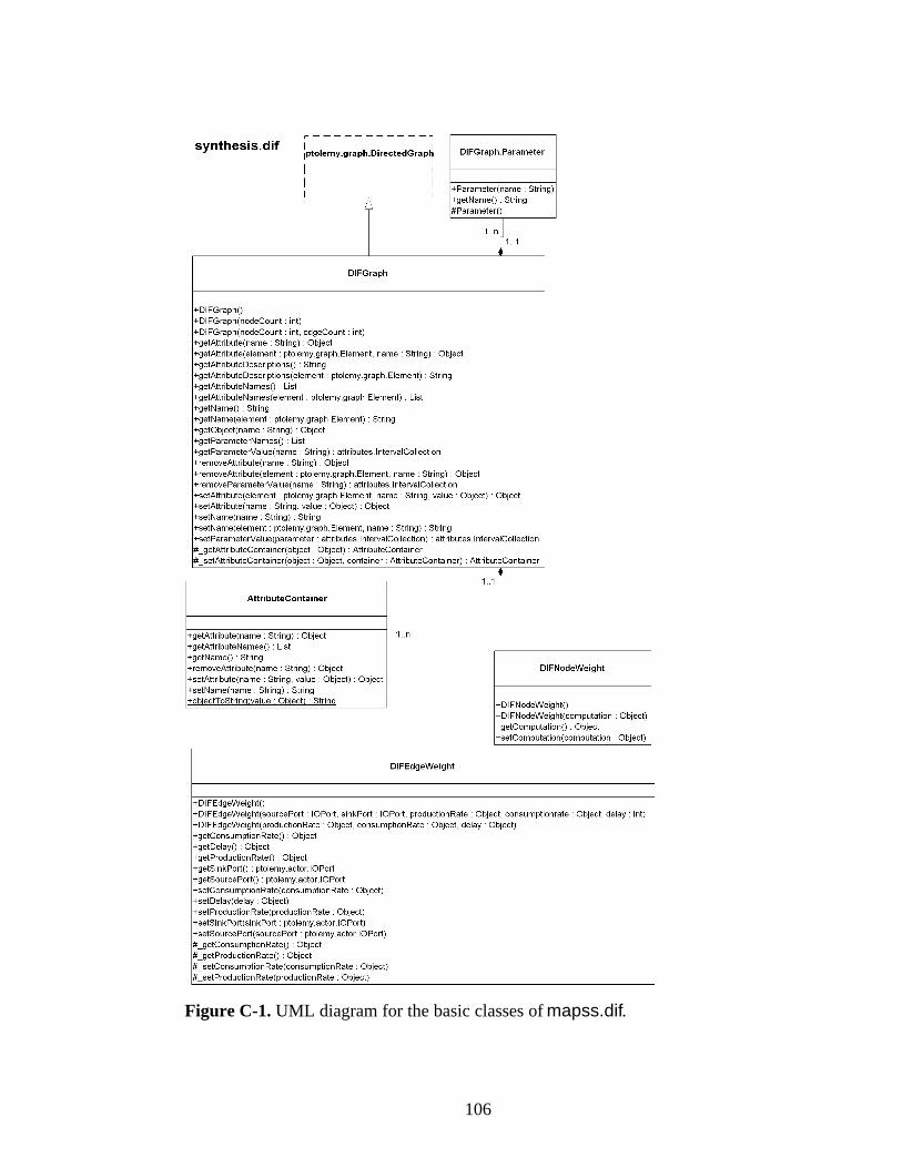
106
Figure C-1. UML diagram for the basic classes of mapss.dif.
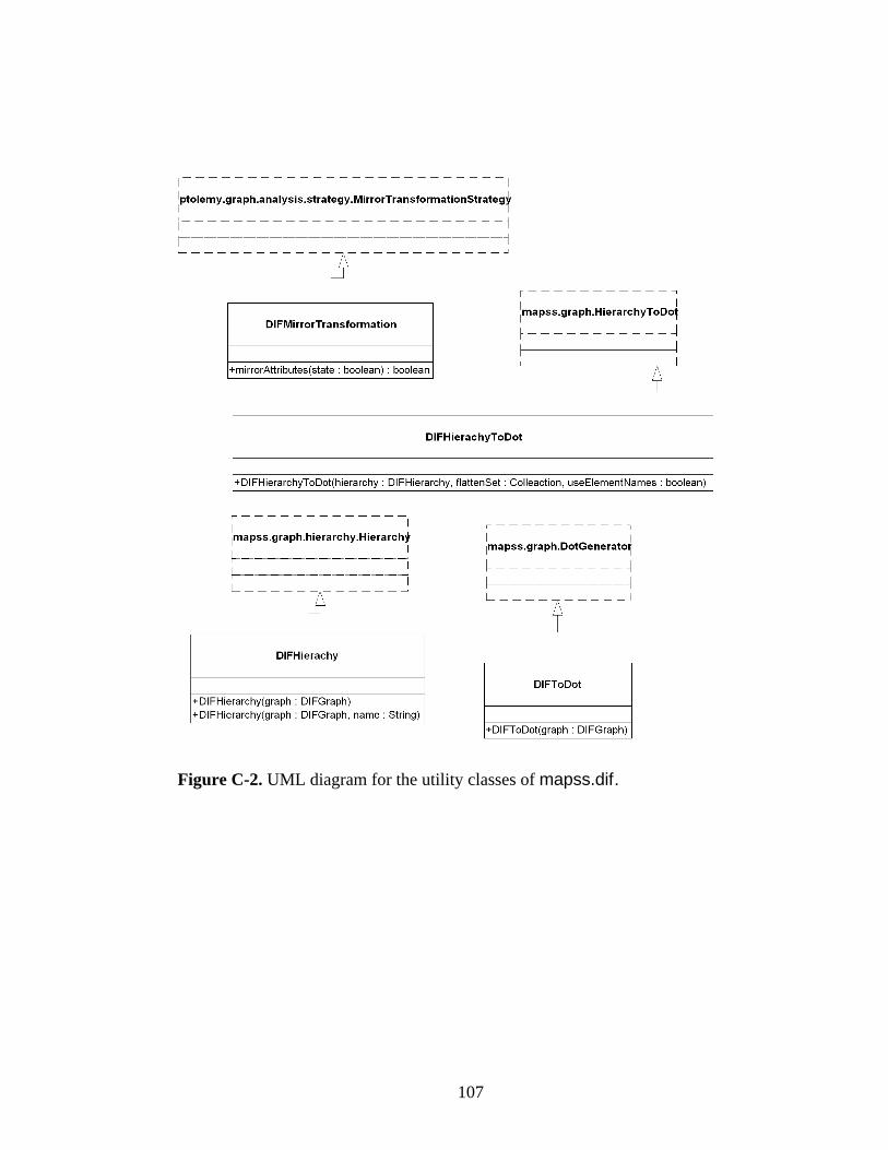
107
Figure C-2. UML diagram for the utility classes of mapss.dif.
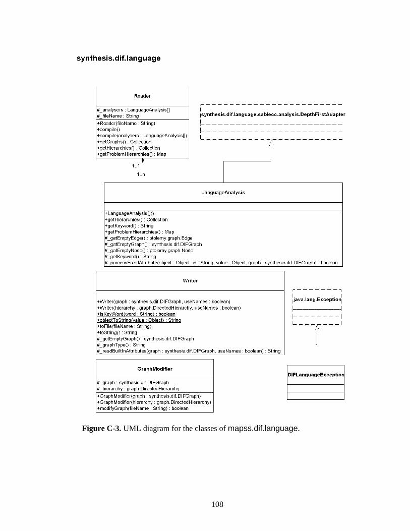
108
Figure C-3. UML diagram for the classes of mapss.dif.language.
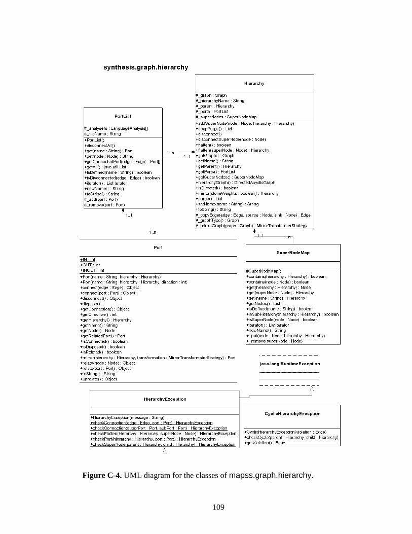
109
Figure C-4. UML diagram for the classes of mapss.graph.hierarchy.
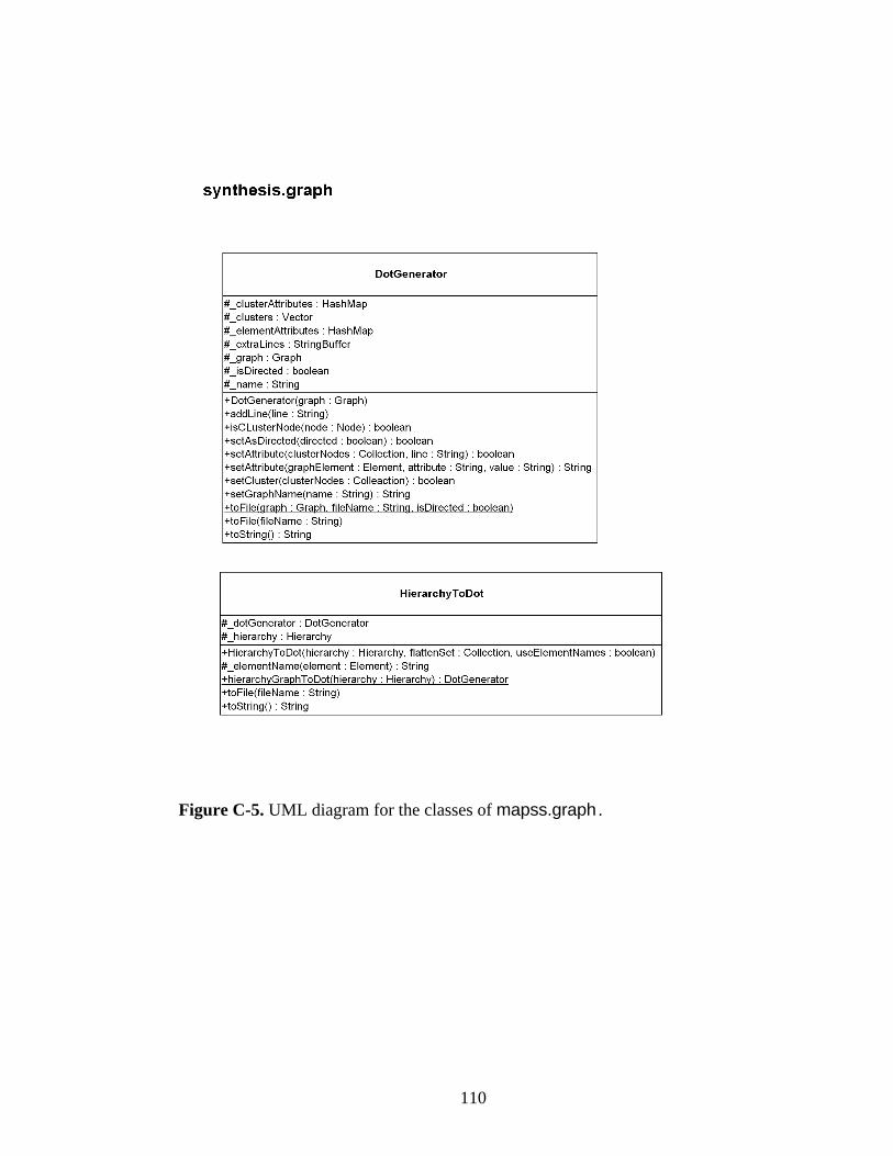
110
Figure C-5. UML diagram for the classes of mapss.graph .
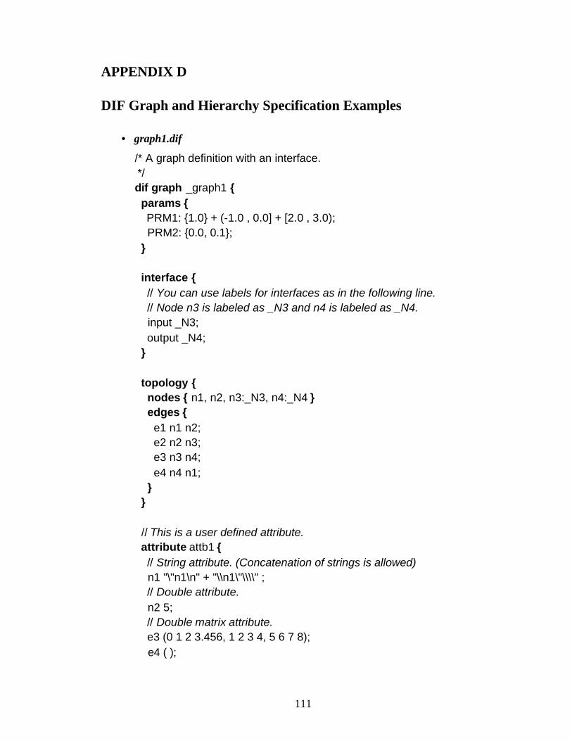
111
APPENDIX D
DIF Graph and Hierarchy Specification Examples
• graph1.dif
/* A graph definition with an interface. */dif graph _graph1 { params { PRM1: {1.0} + (-1.0 , 0.0] + [2.0 , 3.0); PRM2: {0.0, 0.1}; }
interface { // You can use labels for interfaces as in the following line. // Node n3 is labeled as _N3 and n4 is labeled as _N4. input _N3; output _N4; }
topology { nodes { n1, n2, n3:_N3, n4:_N4 } edges { e1 n1 n2; e2 n2 n3; e3 n3 n4; e4 n4 n1; } }
// This is a user defined attribute. attribute attb1 { // String attribute. (Concatenation of strings is allowed) n1 "\"n1\n" + "\\n1\"\\\\" ; // Double attribute. n2 5; // Double matrix attribute. e3 (0 1 2 3.456, 1 2 3 4, 5 6 7 8); e4 ( );
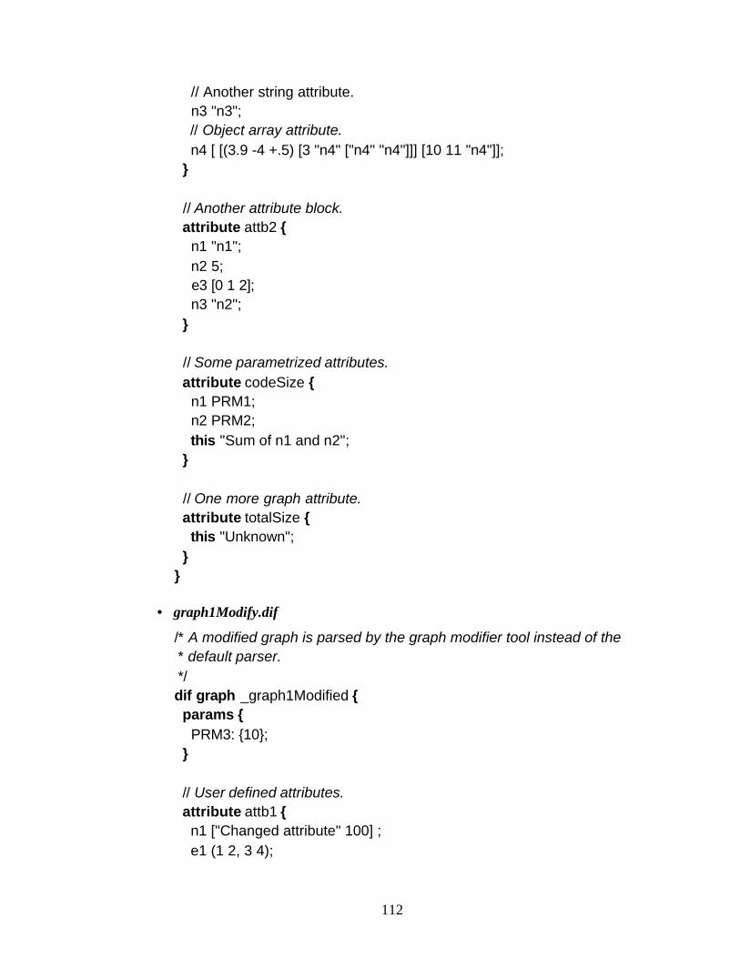
112
// Another string attribute. n3 "n3"; // Object array attribute. n4 [ [(3.9 -4 +.5) [3 "n4" ["n4" "n4"]]] [10 11 "n4"]]; }
// Another attribute block. attribute attb2 { n1 "n1"; n2 5; e3 [0 1 2]; n3 "n2"; }
// Some parametrized attributes. attribute codeSize { n1 PRM1; n2 PRM2; this "Sum of n1 and n2"; }
// One more graph attribute. attribute totalSize { this "Unknown"; }}
• graph1Modify.dif
/* A modified graph is parsed by the graph modifier tool instead of the * default parser. */dif graph _graph1Modified { params { PRM3: {10}; }
// User defined attributes. attribute attb1 { n1 ["Changed attribute" 100] ; e1 (1 2, 3 4);
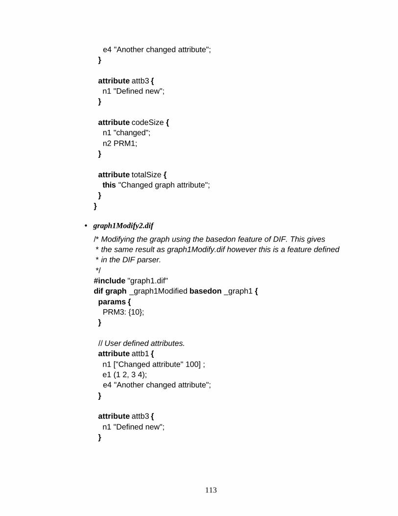
113
e4 "Another changed attribute"; }
attribute attb3 { n1 "Defined new"; }
attribute codeSize { n1 "changed"; n2 PRM1; }
attribute totalSize { this "Changed graph attribute"; }}
• graph1Modify2.dif
/* Modifying the graph using the basedon feature of DIF. This gives * the same result as graph1Modify.dif however this is a feature defined * in the DIF parser. */#include "graph1.dif"dif graph _graph1Modified basedon _graph1 { params { PRM3: {10}; }
// User defined attributes. attribute attb1 { n1 ["Changed attribute" 100] ; e1 (1 2, 3 4); e4 "Another changed attribute"; }
attribute attb3 { n1 "Defined new"; }
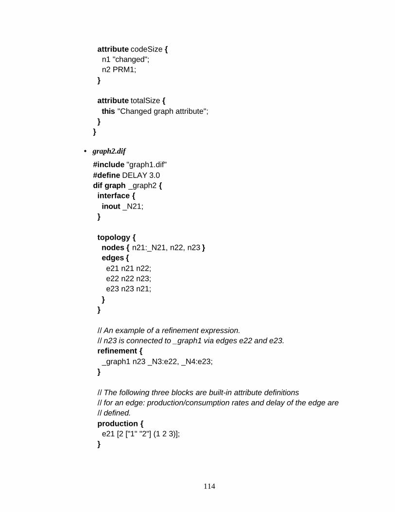
114
attribute codeSize { n1 "changed"; n2 PRM1; }
attribute totalSize { this "Changed graph attribute"; }}
• graph2.dif
#include "graph1.dif"#define DELAY 3.0dif graph _graph2 { interface { inout _N21; }
topology { nodes { n21:_N21, n22, n23 } edges { e21 n21 n22; e22 n22 n23; e23 n23 n21; } }
// An example of a refinement expression. // n23 is connected to _graph1 via edges e22 and e23. refinement { _graph1 n23 _N3:e22, _N4:e23; }
// The following three blocks are built-in attribute definitions // for an edge: production/consumption rates and delay of the edge are // defined. production { e21 [2 ["1" "2"] (1 2 3)]; }
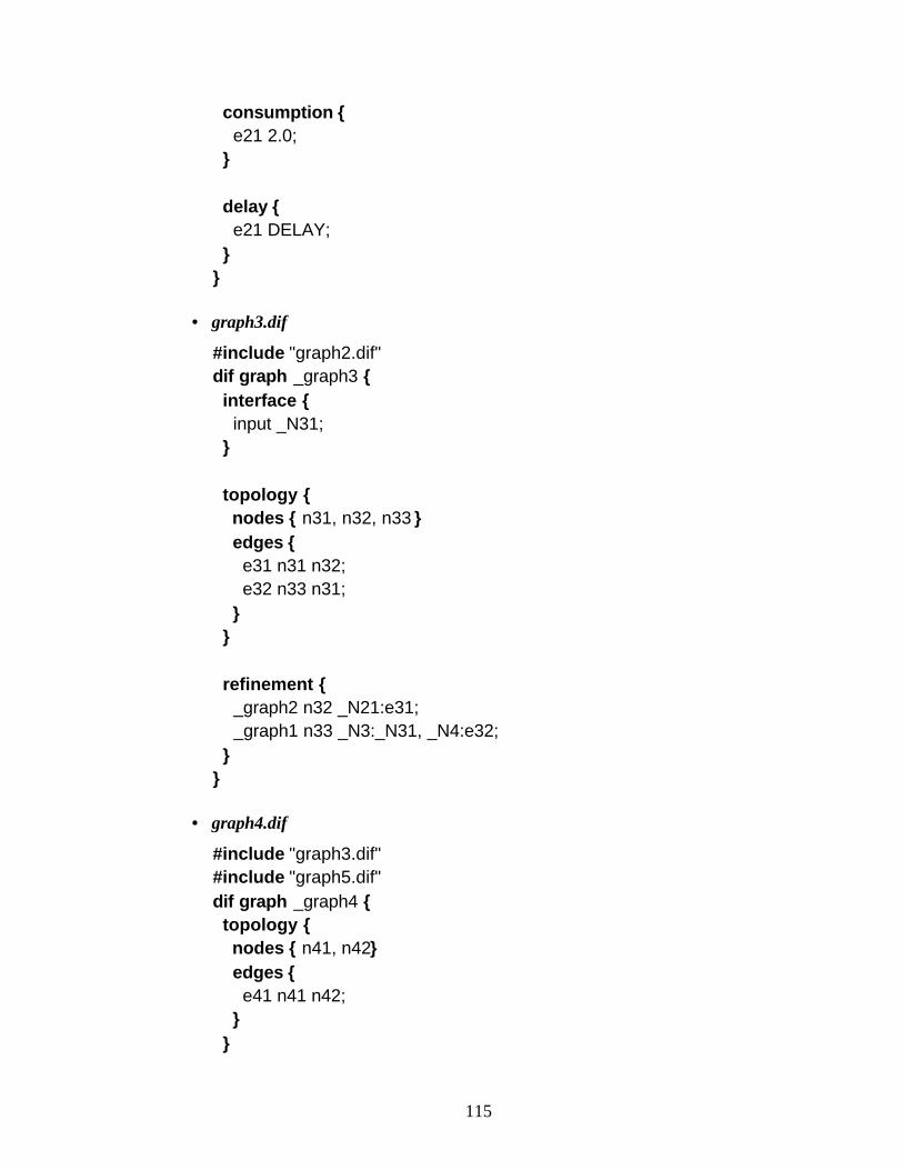
115
consumption { e21 2.0; }
delay { e21 DELAY; }}
• graph3.dif
#include "graph2.dif"dif graph _graph3 { interface { input _N31; }
topology { nodes { n31, n32, n33 } edges { e31 n31 n32; e32 n33 n31; } }
refinement { _graph2 n32 _N21:e31; _graph1 n33 _N3:_N31, _N4:e32; }}
• graph4.dif
#include "graph3.dif"#include "graph5.dif"dif graph _graph4 { topology { nodes { n41, n42} edges { e41 n41 n42; } }
116
refinement { _graph3 n42 _N31:e41; _graph5 n41 _N51:e41; }}
• graph5.dif
sdf graph _graph5 { interface { output _N51; }
topology { nodes { n51:_N51} }}
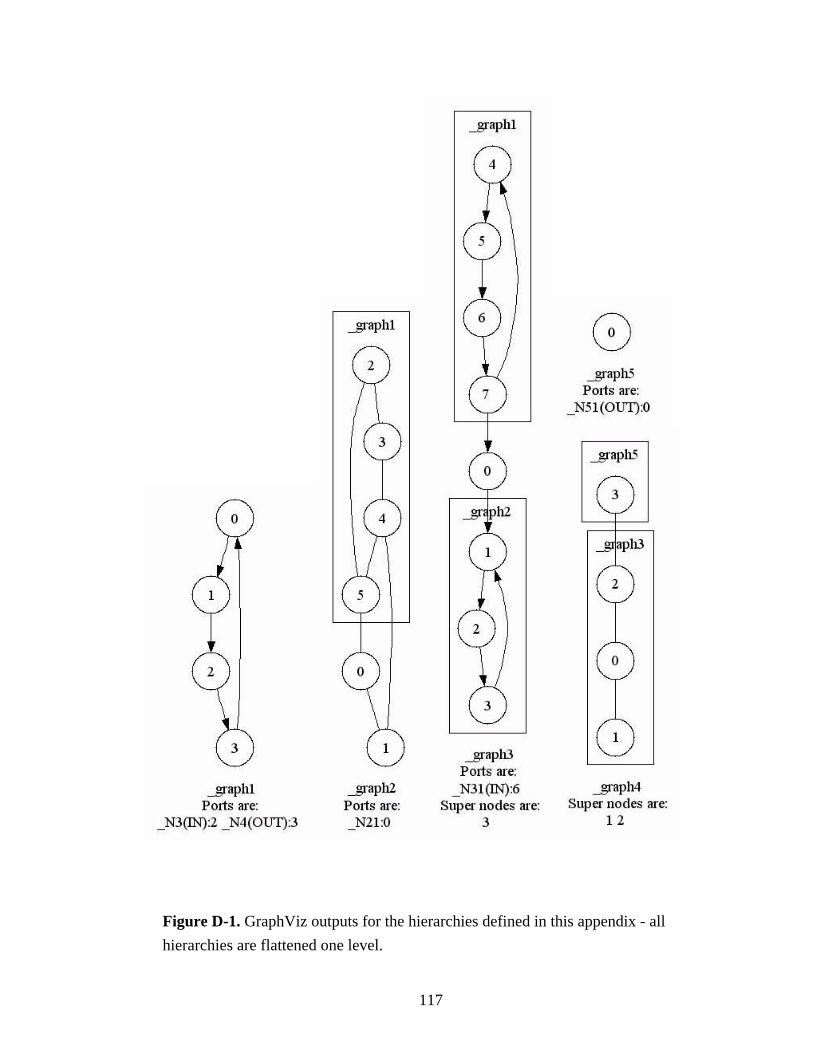
117
Figure D-1. GraphViz outputs for the hierarchies defined in this appendix - all hierarchies are flattened one level.
118
[1] Peter Naur, Revised Report on the Algorithmic Language ALGOL 60. Communica-tions of the ACM, Vol. 3 No.5, pp. 299-314, May 1960
[2] B. Bhattacharya and S. S. Bhattacharyya. Parameterized dataflow modeling for DSPsystems. IEEE Transactions on Signal Processing, 49(10):2408-2421, October2001.
[3] S. S. Bhattacharyya, R. Leupers, and P. Marwedel. Software synthesis and code gen-eration for DSP. IEEE Transactions on Circuits and Systems — II: Analog and Digi-tal Signal Processing, 47(9):849-875, September 2000.
[4] S. S. Bhattacharyya, P. K. Murthy, and E. A. Lee. Synthesis of embedded softwarefrom synchronous dataflow specifications. Journal of VLSI Signal Processing Sys-tems for Signal, Image, and Video Technology, 21(2):151-166, June 1999.
[5] G. Bilsen, M. Engels, R. Lauwereins, and J. A. Peperstraete. Cyclo-static data flow.In Proc. ICASSP, pages 3255-3258, May 1995.
[6] J. T. Buck and E. A. Lee. Scheduling dynamic dataflow graphs using the token flowmodel. In Proc. ICASSP, April 1993.
[7] E. Gagnon. SableCC, an object-oriented compiler framework. Master's thesis,School of Computer Science, McGill University, Montreal, Canada, March 1998.
[8] G. R. Gao, R. Govindarajan, and P. Panangaden. Well-behaved programs for DSPcomputation. In Proc. ICASSP, March 1992.
[9] K. Ito and K. K. Parhi. Determining the iteration bounds of single-rate and multi-rate data-flow graphs. In Proc. IEEE Asia-Pacific Conference on Circuits and Sys-tems, December 1994.
[10] E. Koutsofios and S. C. North. dot user's manual. Technical report, AT&T Bell Lab-oratories, November 1996.
[11] E. A. Lee. Overview of the Ptolemy project. Technical Report UCB/ERL M01/11,Department of EECS, UC Berkeley, March 2001.
[12] E. A. Lee and D. G. Messerschmitt. Synchronous dataflow. Proceedings of theIEEE, 75(9):1235-1245, September 1987.
119
[13] M. Pankert, O. Mauss, S. Ritz, and H. Meyr. Dynamic data flow and control flow inhigh level DSP code synthesis. In Proc. ICASSP, 1994.
[14] C. B. Robbins. Autocoding Toolset software tools for automatic generation of paral-lel application software. Technical report, Management, Communications & Con-trol, Inc., 2002.
[15] G. C. Sih. Multiprocessor Scheduling to account for Interprocessor Communication.Ph.D. thesis, Department of EECS, UC Berkeley, April 1991.
[16] B. Kernighan, D. Ritchie, The C Programming Language, 2nd Edition. PrenticeHall, 1988.
[17] G. Bracha, J. Gosling, B. Joy and G. Steele, The Java Language Specification, 2ndEdition. Addison-Wesley, 2000.