1

Dataflow AnalysisDataflow AnalysisWidening and NarrowingWidening and Narrowing

Path SensitivityPath SensitivityInterprocedural AnalysisInterprocedural Analysis

Static Analysis 2009Static Analysis 2009

Michael I. SchwartzbachComputer Science, University of Aarhus

2

2Static Analysis

Sign AnalysisSign Analysis

Determine the sign (+,-,0) of all expressionsThe Sign lattice:

The full lattice is the map lattice: Vars → Sign• where Vars is the set of variables in the program

?

+ - 0

3

3Static Analysis

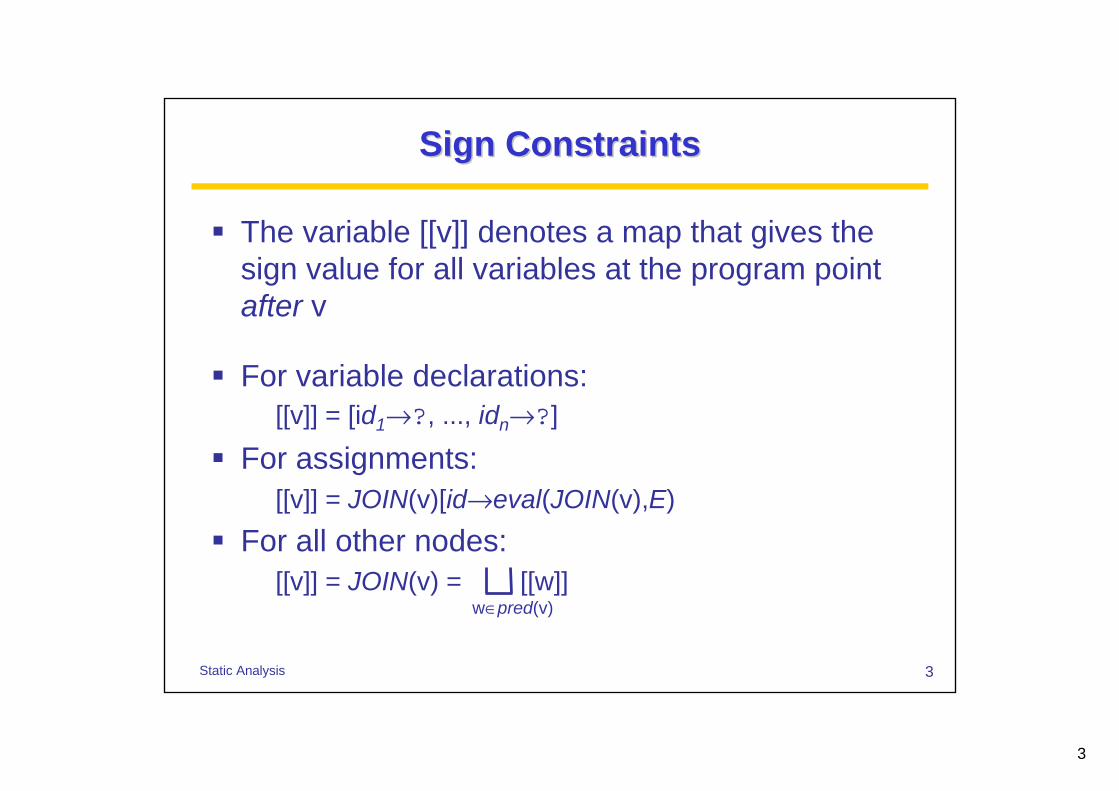
Sign ConstraintsSign Constraints

The variable [[v]] denotes a map that gives the sign value for all variables at the program point after v

For variable declarations:[[v]] = [id1→?, ..., idn→?]

For assignments:[[v]] = JOIN(v)[id→eval(JOIN(v),E)

For all other nodes:[[v]] = JOIN(v) = [[w]]

w∈pred(v)

4

4Static Analysis

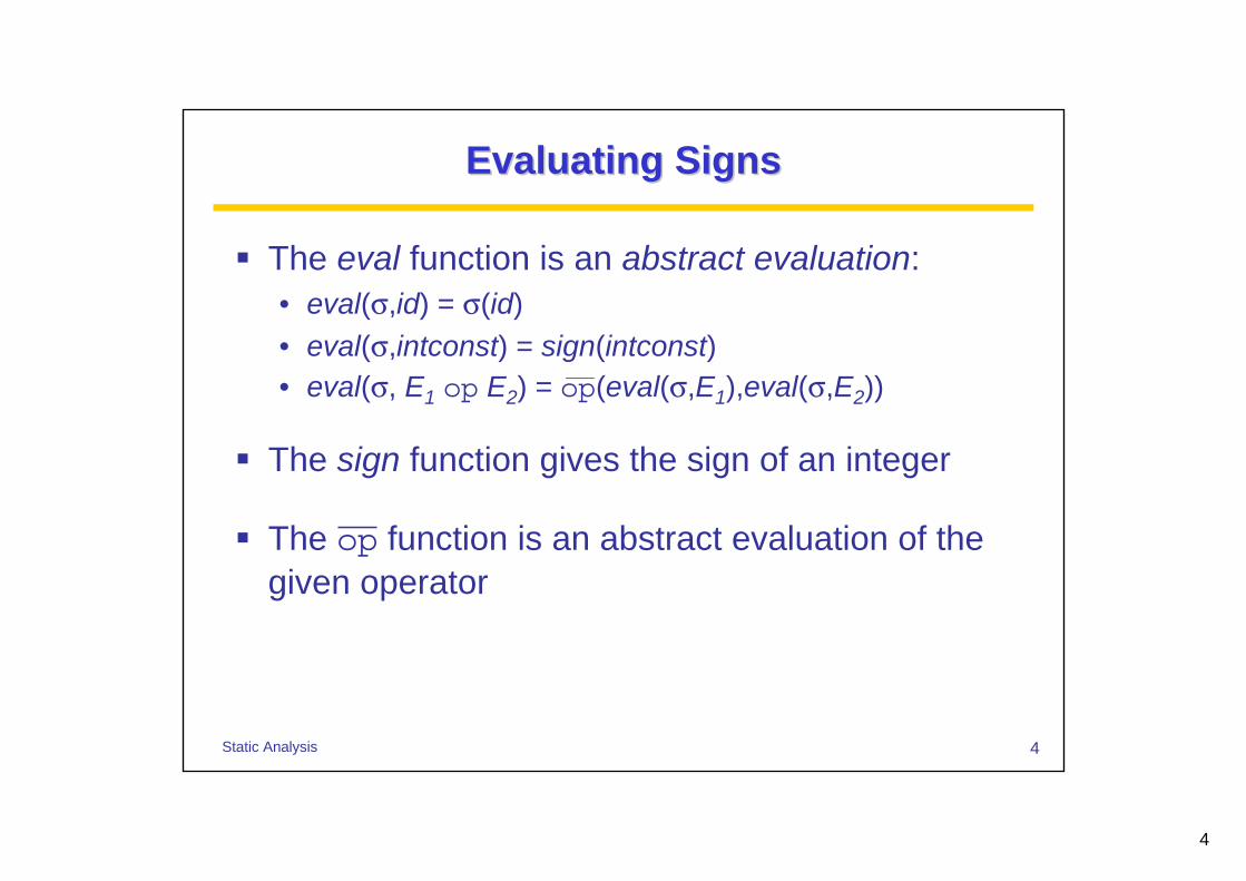
Evaluating SignsEvaluating Signs

The eval function is an abstract evaluation:• eval(σ,id) = σ(id)• eval(σ,intconst) = sign(intconst)• eval(σ, E1 op E2) = op(eval(σ,E1),eval(σ,E2))

The sign function gives the sign of an integer

The op function is an abstract evaluation of the given operator

5

5Static Analysis

Abstract OperatorsAbstract Operators

????⊥?

?+?+⊥+

??--⊥-

?+-0⊥0

⊥⊥⊥⊥⊥⊥

?+-0⊥+

????⊥?

??++⊥+

?-?-⊥-

?-+0 ⊥0

⊥⊥⊥⊥⊥⊥

?+-0⊥-

???0⊥?

?+-0⊥+

?-+0⊥-

000000

⊥⊥⊥0⊥⊥

?+-0⊥*

????⊥?

????⊥+

????⊥-

?00?⊥0

⊥⊥⊥⊥⊥⊥

?+-0⊥/

????⊥?

??++⊥+

?0?0⊥-

?0+0⊥0

⊥⊥⊥⊥⊥⊥

?+-0⊥>

????⊥?

??00⊥+

?0?0⊥-

?00+⊥0

⊥⊥⊥⊥⊥⊥

?+-0⊥==

6

6Static Analysis

MonotonicityMonotonicity

The operator and map updates are monotoneCompositions preserve monotonicityAre the abstract operators monotone?

This is verified by a tedious manual inspectionOr better, run an O(n3) algorithm for an n×n table:• ∀x,y,x’∈L: x x’ ⇒ x op y x’ op y• ∀x,y,y’∈L: y y’ ⇒ x op y x op y’

7

7Static Analysis

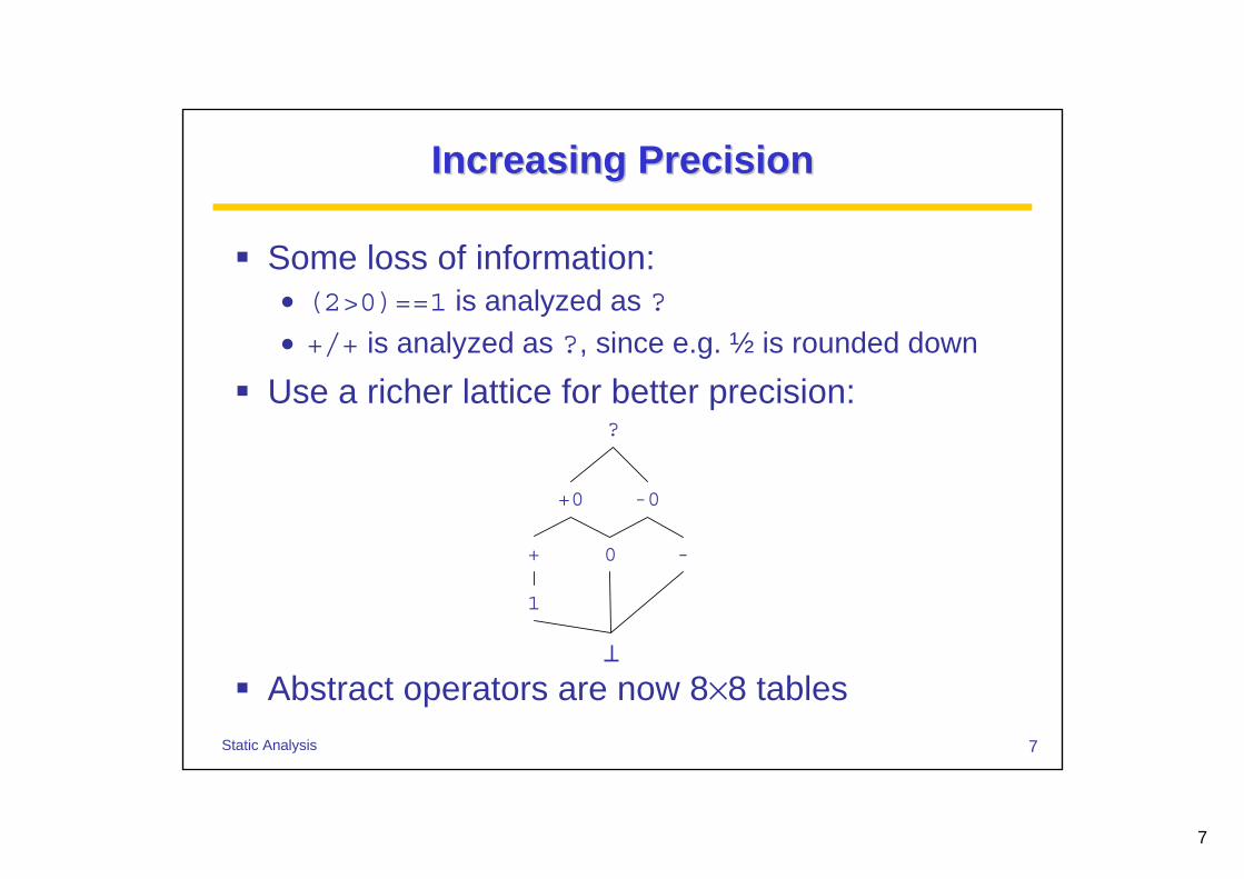
Increasing PrecisionIncreasing Precision

Some loss of information:• (2>0)==1 is analyzed as ?• +/+ is analyzed as ?, since e.g. ½ is rounded down

Use a richer lattice for better precision:

Abstract operators are now 8×8 tables

?

+ 0 -

1

+0 -0

8

8Static Analysis

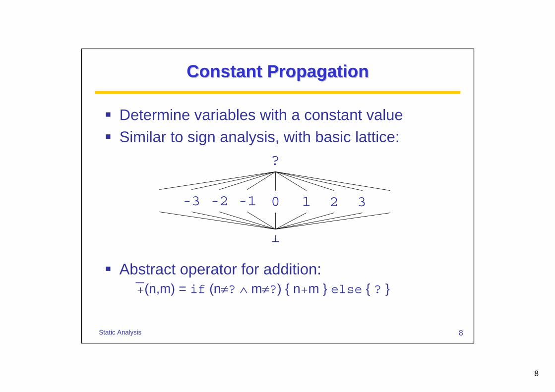
Constant PropagationConstant Propagation

Determine variables with a constant valueSimilar to sign analysis, with basic lattice:

Abstract operator for addition:+(n,m) = if (n≠? ∧ m≠?) { n+m } else { ? }

?

-1 0 1 2 3-2-3

9

9Static Analysis

Constant FoldingConstant Folding

Exploiting constant propagation:var x,y,z;

x = 27;

y = input,

z = 2*x+y;

if (x<0) { y=z-3; } else { y=12 }

output y;

var x,y,z; var y;

x = 27; y = input;

y = input; output 12;

z = 54+y;

if (0) { y=z-3; } else { y=12 }

output y;

10

10Static Analysis

Interval AnalysisInterval Analysis

Compute upper and lower bounds for integersLattice of intervals:

Interval = lift({ [l,h] | l,h ∈N ∧ l ≤ h })where:

N = {-∞, ..., -2, -1, 0, 1, 2, ..., ∞}and intervals are ordered by inclusion:

[l1,h1] [l2,h2] iff l2 ≤ l1 ∧ h1 ≤ h2

11

11Static Analysis

The Interval LatticeThe Interval Lattice

[-∞,∞]

[0,0] [1,1] [2,2][-1,-1][-2,-2]

[0,1] [1,2][-1,0][-2,-1]

[2,∞]

[1,∞]

[0,∞]

[-∞,-2]

[-∞,-1]

[-∞,0]

[-2,0] [-1,1] [0,2]

[-2,1] [-1,2]

[-2,2]

⊥

12

12Static Analysis

Interval Analysis LatticeInterval Analysis Lattice

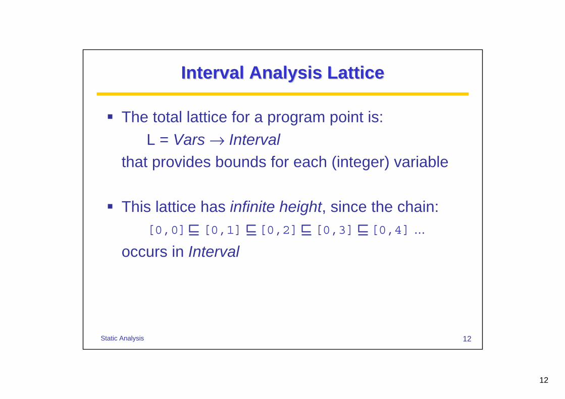
The total lattice for a program point is:L = Vars → Interval

that provides bounds for each (integer) variable

This lattice has infinite height, since the chain:[0,0] [0,1] [0,2] [0,3] [0,4] ...

occurs in Interval

13

13Static Analysis

Interval ConstraintsInterval Constraints

For the entry node:[[entry]] = λx.[-∞,∞]

For assignments:[[v]] = JOIN(v)[id→eval(JOIN(v),E))

For all other nodes:[[v]] = JOIN(v) = [[w]]

w∈pred(v)

14

14Static Analysis

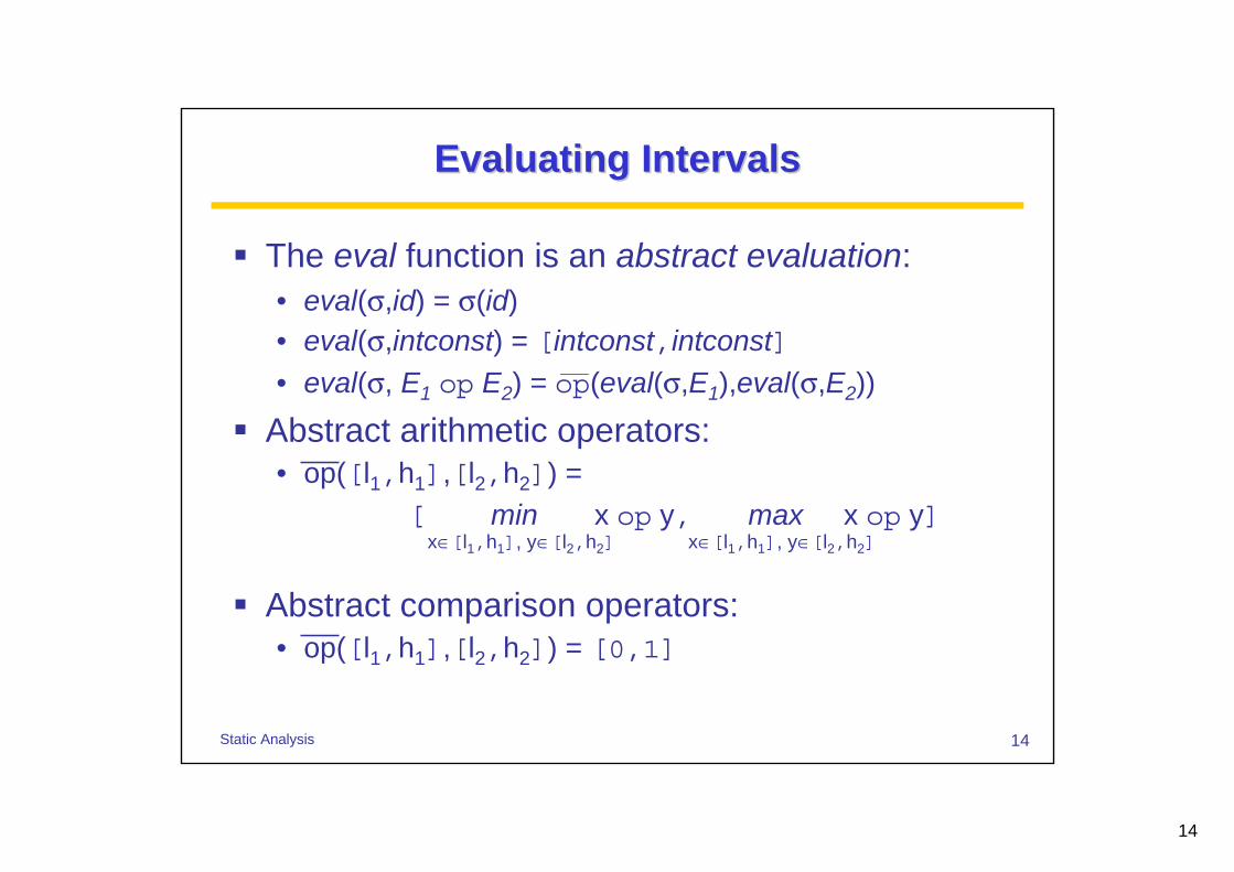
Evaluating IntervalsEvaluating Intervals

The eval function is an abstract evaluation:• eval(σ,id) = σ(id)• eval(σ,intconst) = [intconst,intconst]• eval(σ, E1 op E2) = op(eval(σ,E1),eval(σ,E2))

Abstract arithmetic operators:• op([l1,h1],[l2,h2]) =

[ min x op y, max x op y]

Abstract comparison operators:• op([l1,h1],[l2,h2]) = [0,1]

x∈[l1,h1], y∈[l2,h2] x∈[l1,h1], y∈[l2,h2]

15

15Static Analysis

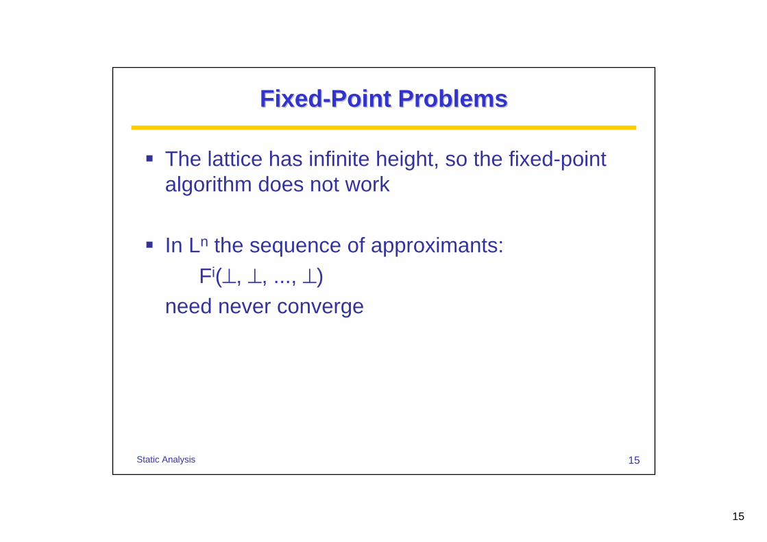
FixedFixed--Point ProblemsPoint Problems

The lattice has infinite height, so the fixed-point algorithm does not work

In Ln the sequence of approximants:Fi(⊥, ⊥, ..., ⊥)

need never converge

16

16Static Analysis

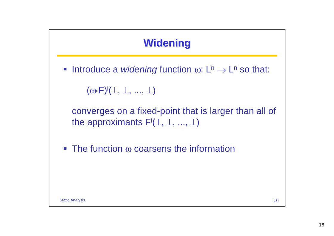
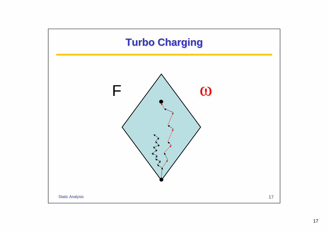
WideningWidening

Introduce a widening function ω: Ln → Ln so that:

(ω F)i(⊥, ⊥, ..., ⊥)

converges on a fixed-point that is larger than all of the approximants Fi(⊥, ⊥, ..., ⊥)

The function ω coarsens the information

17

17Static Analysis

Turbo ChargingTurbo Charging

F ω

18

18Static Analysis

Widening for IntervalsWidening for Intervals

The function ω is defined pointwiseParameterized with a fixed finite subset B⊂N• must contain -∞ and ∞• typically seeded with all integer constants occurring in

the given programOn single intervals:

ω([l,h]) = [ max{i∈B|i≤l}, min{i∈B|h≤i} ]

Finds the nearest enclosing allowed interval

19

19Static Analysis

Correctness of WideningCorrectness of Widening

Widening works when:• ω is an increasing and monotone function• ω(L) is a finite lattice

Fi(⊥, ⊥, ..., ⊥) (ω F)i(⊥, ⊥, ..., ⊥)since F is monotone and ω is increasing

ω F is a monotone function ω(L)→ω(L)so the fixed-point exists

20

20Static Analysis

NarrowingNarrowing

Widening shoots over the targetNarrowing may improve the result by applying FDefine:

fix = Fi(⊥, ⊥, ..., ⊥) fixω = (ω F)i(⊥, ⊥, ..., ⊥)

then fix fixωBut we also have that:

fix F(fixω) fixω

so applying F again may improve the resultThis can be iterated arbitrarily many times

21

21Static Analysis

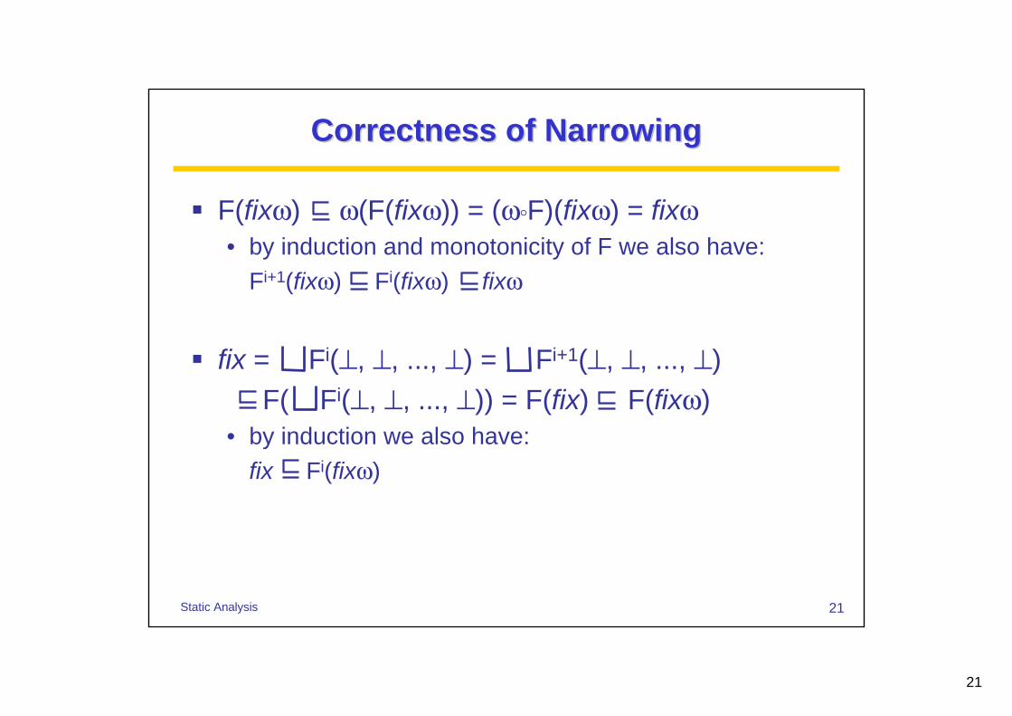
Correctness of NarrowingCorrectness of Narrowing

F(fixω) ω(F(fixω)) = (ω F)(fixω) = fixω• by induction and monotonicity of F we also have:

Fi+1(fixω) Fi(fixω) fixω

fix = Fi(⊥, ⊥, ..., ⊥) = Fi+1(⊥, ⊥, ..., ⊥) F( Fi(⊥, ⊥, ..., ⊥)) = F(fix) F(fixω)

• by induction we also have:fix Fi(fixω)

22

22Static Analysis

Backing UpBacking Up

F ω

23

23Static Analysis

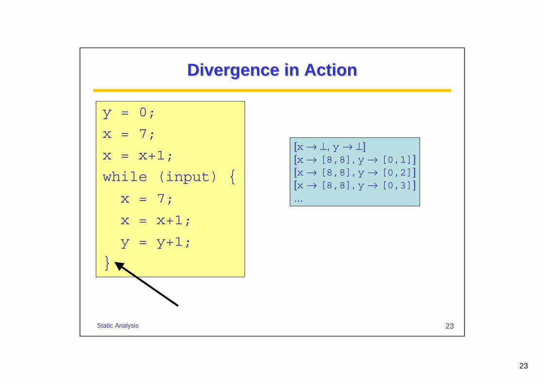
Divergence in ActionDivergence in Action

y = 0;

x = 7;

x = x+1;

while (input) {

x = 7;

x = x+1;

y = y+1;

}

[x → ⊥, y → ⊥][x → [8,8], y → [0,1]][x → [8,8], y → [0,2]][x → [8,8], y → [0,3]]...

24

24Static Analysis

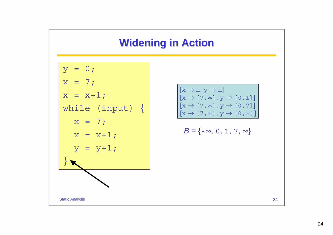
Widening in ActionWidening in Action

y = 0;

x = 7;

x = x+1;

while (input) {

x = 7;

x = x+1;

y = y+1;

}

[x → ⊥, y → ⊥][x → [7,∞], y → [0,1]][x → [7,∞], y → [0,7]][x → [7,∞], y → [0,∞]]

B = {-∞, 0, 1, 7, ∞}

25

25Static Analysis

Narrowing in ActionNarrowing in Action

y = 0;

x = 7;

x = x+1;

while (input) {

x = 7;

x = x+1;

y = y+1;

}

[x → ⊥, y → ⊥][x → [7,∞], y → [0,1]][x → [7,∞], y → [0,7]][x → [7,∞], y → [0,∞]]

[x → [8,8], y → [0,∞]]

B = {-∞, 0, 1, 7, ∞}

26

26Static Analysis

Widening FunctionsWidening Functions

A simple generic widening function:

ω(x) =

A difficult widening function (regular languages):

x if x is small enough

otherwise

∅

Σ*

{a} ⊆ {a,ab} ⊆ {a,ab,abb} ⊆ ... → {ab*}

This is essentially machine learning...

ω

27

27Static Analysis

Information in Conditions Information in Conditions

x = input;

y = 0;

z = 0;

while (x>0) {

z = z+x;

if (17>y) { y = y+1; }

x = x-1;

}

The interval analysis (with widening) concludes:x = [-∞,∞], y = [0,∞], z = [-∞,∞]

28

28Static Analysis

Modeling ConditionsModeling Conditions

Add two artifical statements

The statement assert(E) models that E is truein the current program stateIt causes a runtime error otherwise

The statement refute(E) models that E is falsein the current program stateIt causes a runtime error otherwise

29

29Static Analysis

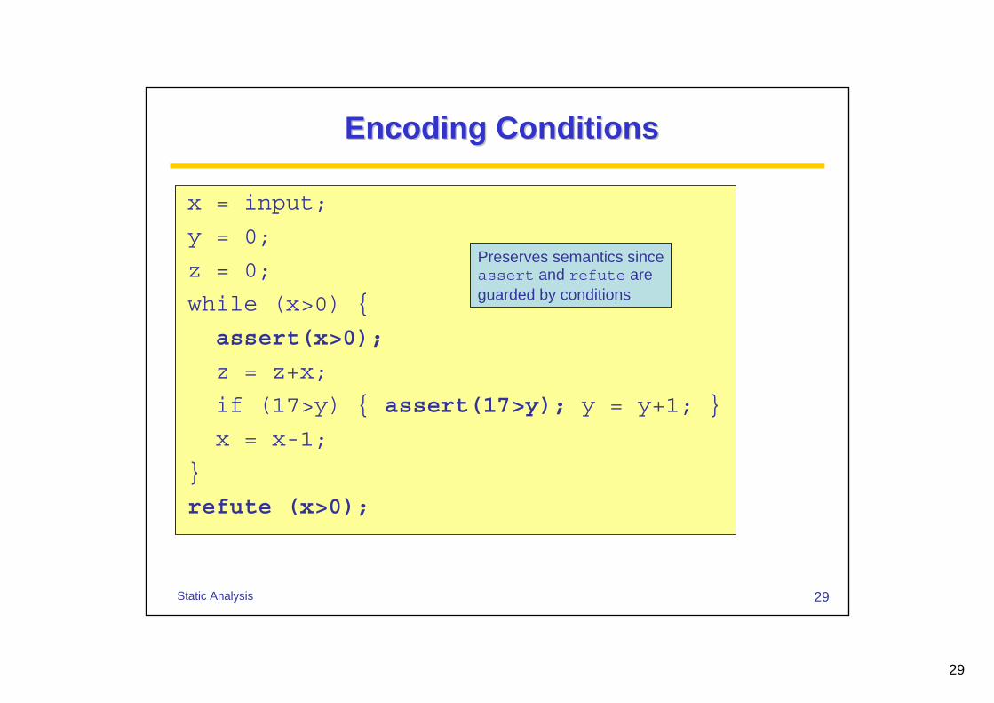
Encoding Conditions Encoding Conditions

x = input;

y = 0;

z = 0;

while (x>0) {

assert(x>0);

z = z+x;

if (17>y) { assert(17>y); y = y+1; }

x = x-1;

}

refute (x>0);

Preserves semantics sinceassert and refute are guarded by conditions

30

30Static Analysis

Constraints for Assert and RefuteConstraints for Assert and Refute

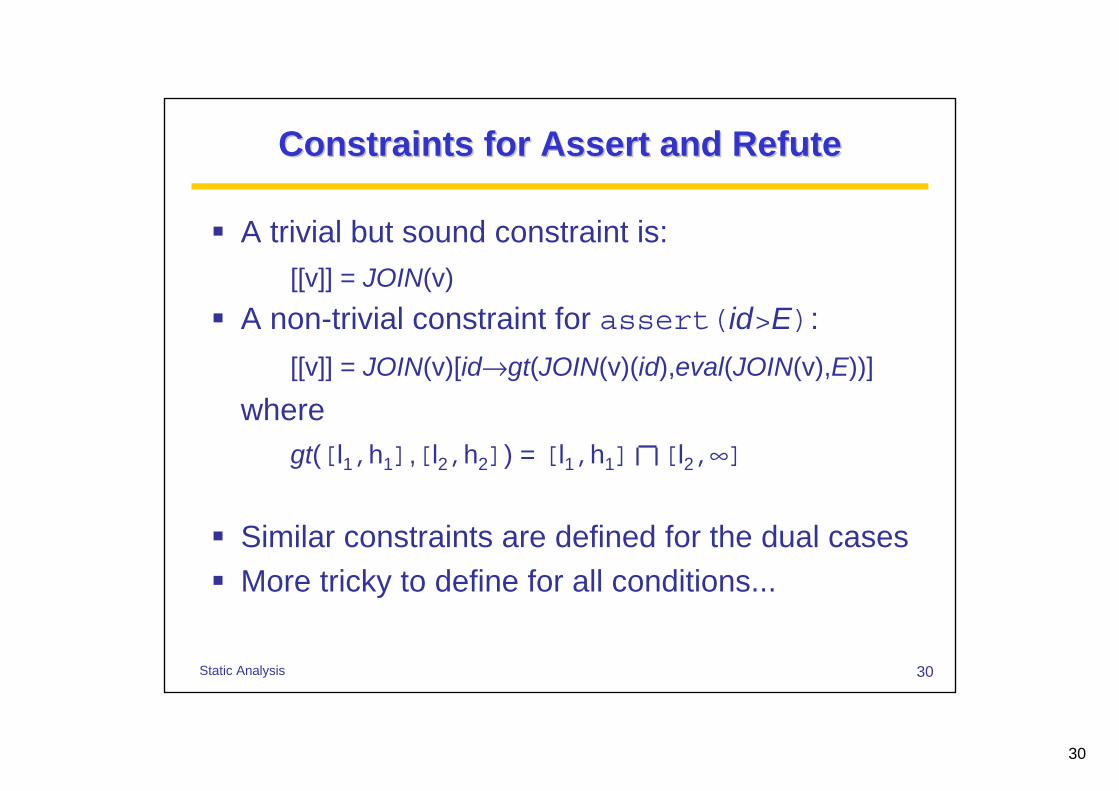
A trivial but sound constraint is:[[v]] = JOIN(v)

A non-trivial constraint for assert(id>E):[[v]] = JOIN(v)[id→gt(JOIN(v)(id),eval(JOIN(v),E))]

wheregt([l1,h1],[l2,h2]) = [l1,h1] [l2,∞]

Similar constraints are defined for the dual casesMore tricky to define for all conditions...

31

31Static Analysis

Exploiting Conditions Exploiting Conditions

x = input;

y = 0;

z = 0;

while (x>0) {

assert(x>0);

z = z+x;

if (17>y) { assert(17>y); y = y+1; }

x = x-1;

}

refute (x>0);

The interval analysis now concludes:x = [-∞,0], y = [0,17], z = [0,∞]

32

32Static Analysis

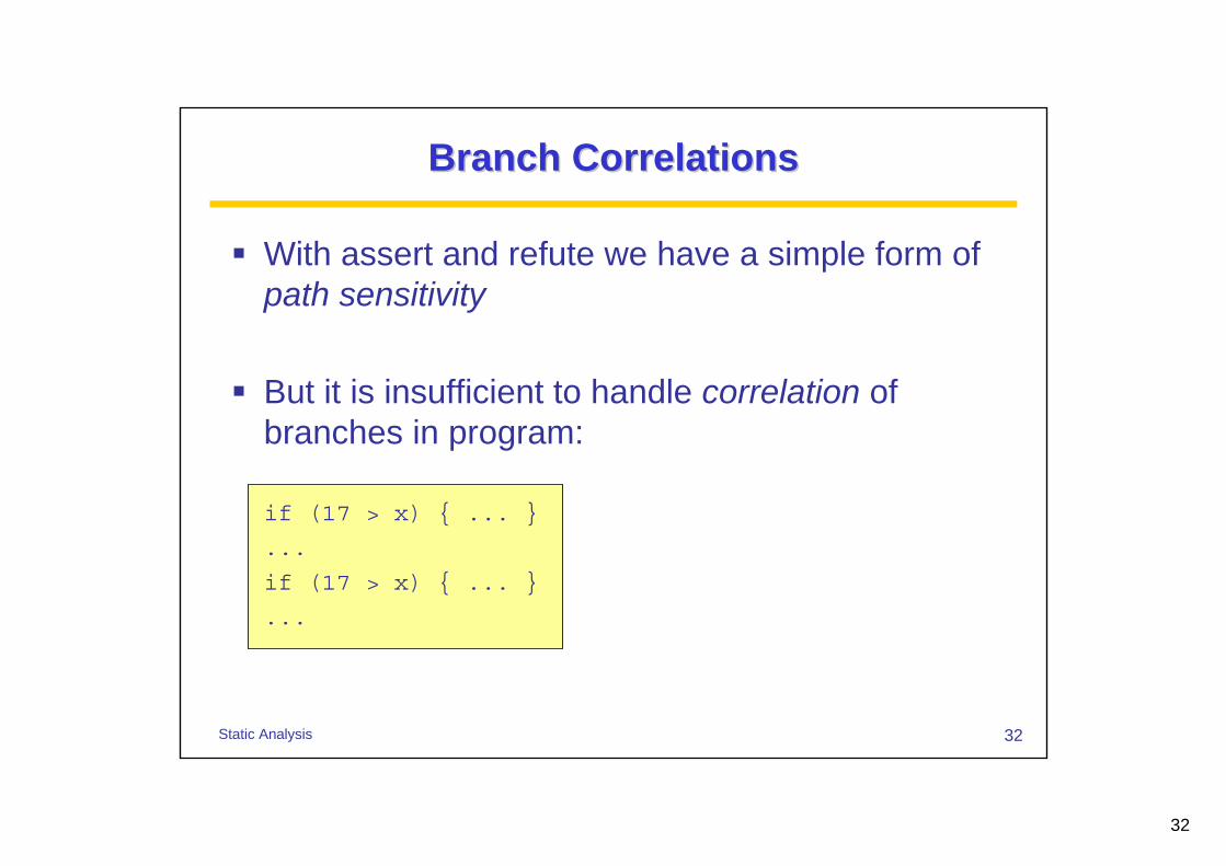
Branch CorrelationsBranch Correlations

With assert and refute we have a simple form of path sensitivity

But it is insufficient to handle correlation of branches in program:

if (17 > x) { ... }

...

if (17 > x) { ... }

...

33

33Static Analysis

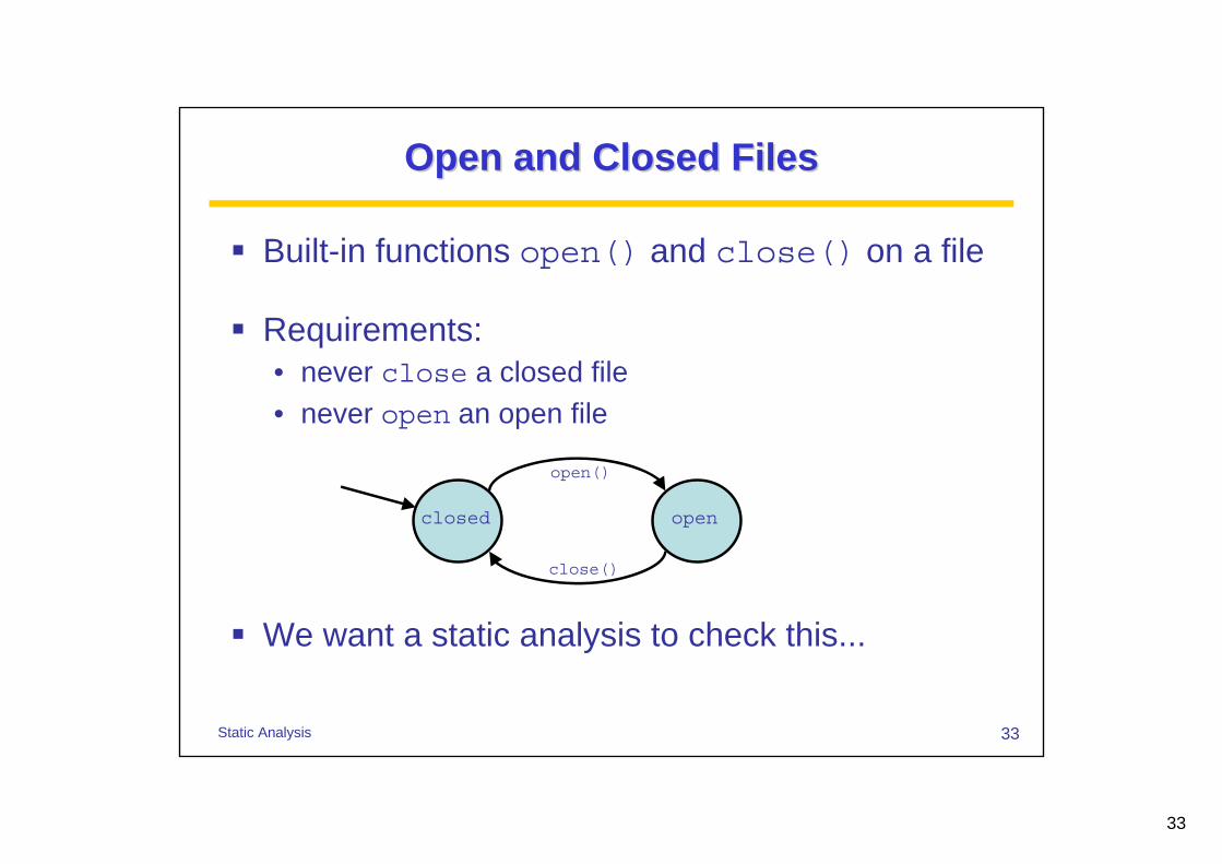
Open and Closed FilesOpen and Closed Files

Built-in functions open() and close() on a file

Requirements:• never close a closed file• never open an open file

We want a static analysis to check this...

openclosed

open()

close()

34

34Static Analysis

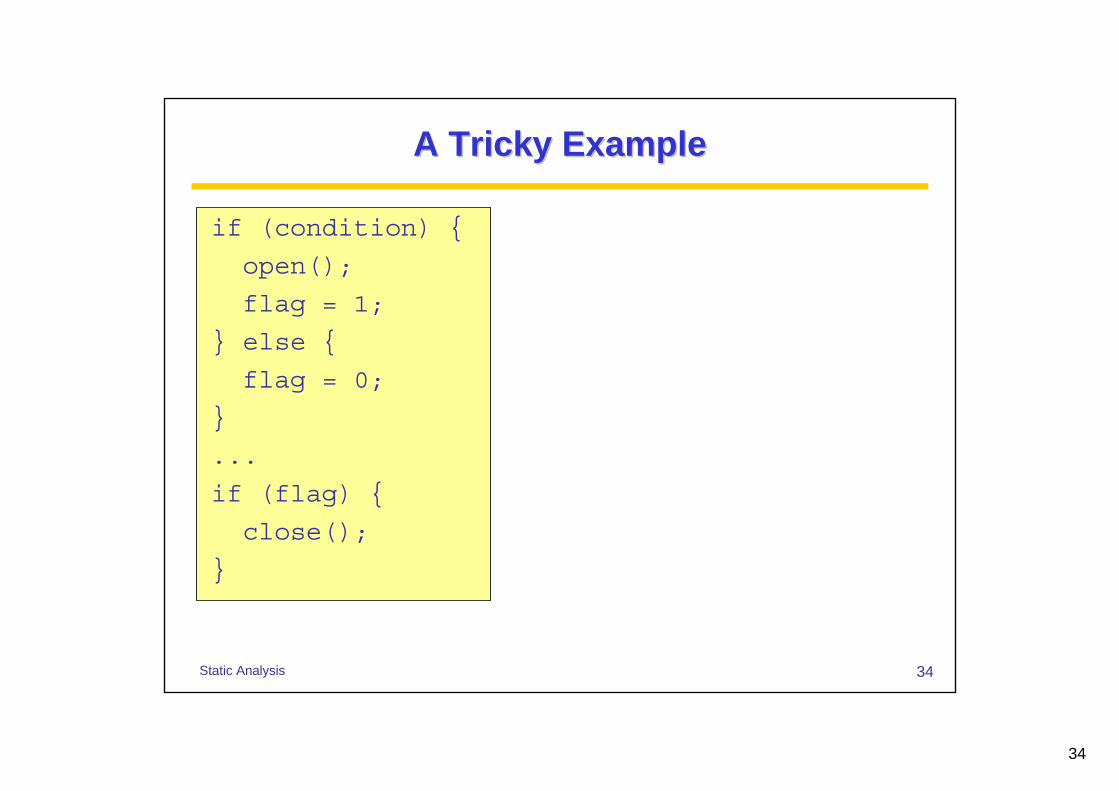
A Tricky ExampleA Tricky Example

if (condition) {

open();

flag = 1;

} else {

flag = 0;

}

...

if (flag) {

close();

}

35

35Static Analysis

The Naive Analysis (1/2)The Naive Analysis (1/2)

The lattice models the status of the file:

L = (2{open,closed},⊆)

For every CFG node, v, we have a constraint variable [[v]] denoting the status after v

JOIN(v) = [[w]]

{open,closed}

{open} {closed}

∅

∪w∈pred(v)

36

36Static Analysis

The Naive Analysis (2/2)The Naive Analysis (2/2)

Constraints for interesting statements:[[entry]] = {closed}[[open()]] = {open}[[close()]] = {closed}

For all other CFG nodes:[[v]] = JOIN(v)

Before the close() statement the analysis concludes that the file is {open,closed}

37

37Static Analysis

Context AwarenessContext Awareness

We need to keep track of the flag variableOur second attempt is the lattice:

L = (2{open,closed}×2{flag=0,flag≠0},⊆×⊆)

Additionally, we add assert(...) and refute(...) to keep track of conditionals

Even so, we now only now that the file is {open,closed} and that flag is {flag=0,flag≠0}

38

38Static Analysis

Relational AnalysisRelational Analysis

We need an analysis that keeps track of relationsbetween variables

This requires that we maintain multiple abstract states per program point, one for each context

For the file example we need the lattice:

L = C → 2{open,closed}

where C = {flag=0,flag≠0} is the set of contexts

39

39Static Analysis

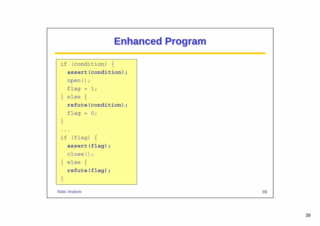
Enhanced ProgramEnhanced Program

if (condition) {

assert(condition);

open();

flag = 1;

} else {

refute(condition);

flag = 0;

}

...

if (flag) {

assert(flag);

close();

} else {

refute(flag);

}

40

40Static Analysis

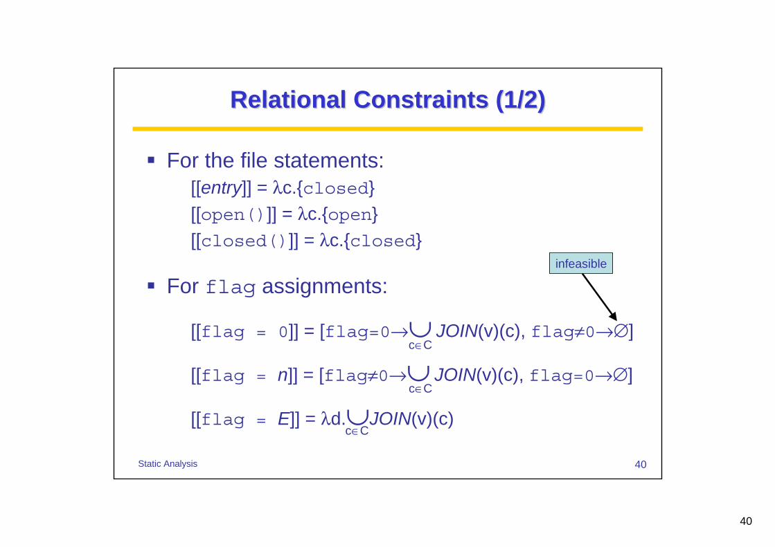
Relational Constraints (1/2)Relational Constraints (1/2)

For the file statements:[[entry]] = λc.{closed}[[open()]] = λc.{open}[[closed()]] = λc.{closed}

For flag assignments:

[[flag = 0]] = [flag=0→∪ JOIN(v)(c), flag≠0→∅]

[[flag = n]] = [flag≠0→∪ JOIN(v)(c), flag=0→∅]

[[flag = E]] = λd.∪JOIN(v)(c)

c∈C

c∈C

infeasible

c∈C

41

41Static Analysis

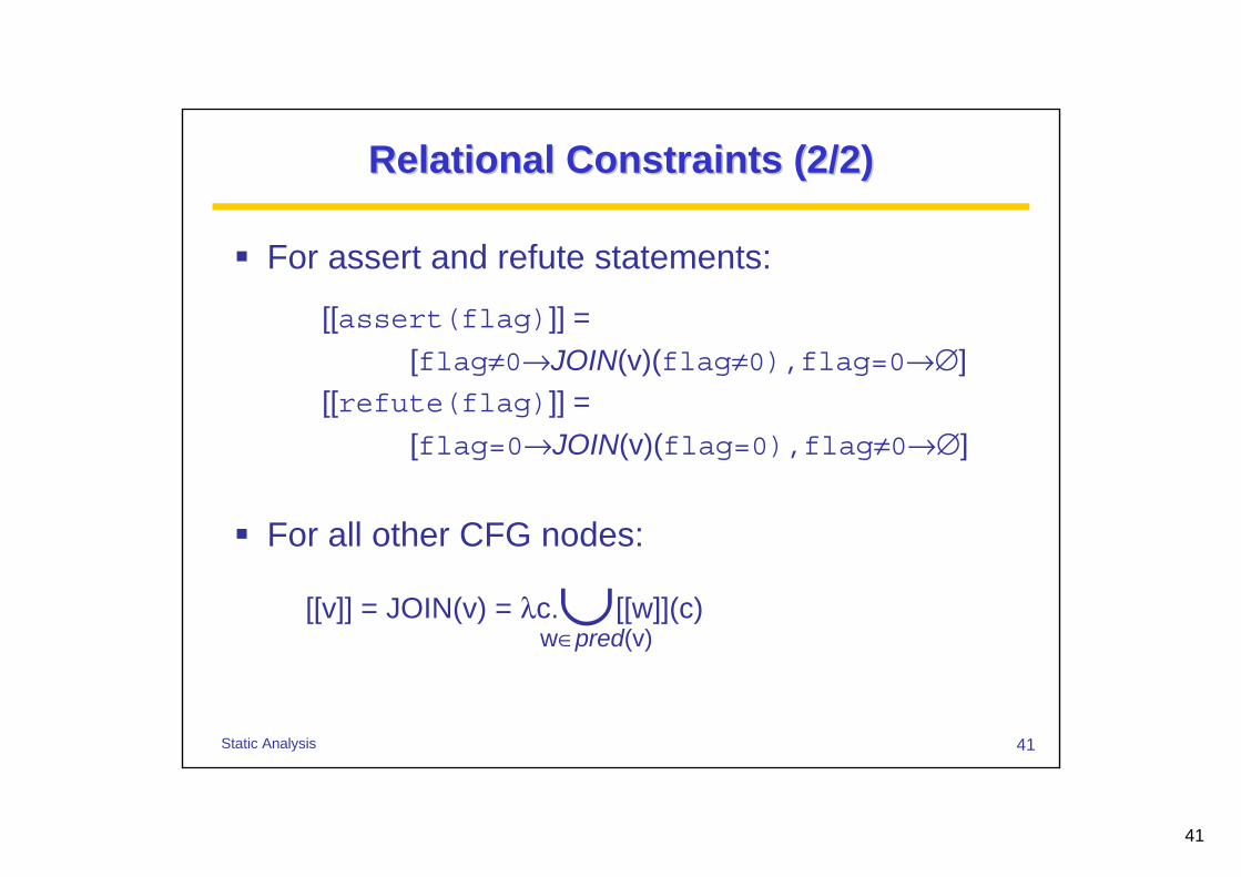
Relational Constraints (2/2)Relational Constraints (2/2)

For assert and refute statements:

[[assert(flag)]] = [flag≠0→JOIN(v)(flag≠0),flag=0→∅]

[[refute(flag)]] = [flag=0→JOIN(v)(flag=0),flag≠0→∅]

For all other CFG nodes:

[[v]] = JOIN(v) = λc. [[w]](c)∪w∈pred(v)

42

42Static Analysis

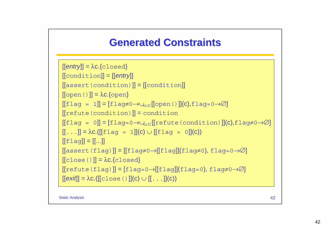
Generated ConstraintsGenerated Constraints

[[entry]] = λc.{closed}[[condition]] = [[entry]][[assert(condition)]] = [[condition]][[open()]] = λc.{open}[[flag = 1]] = [flag≠0→∪ [[open()]](c),flag=0→∅][[refute(condition)]] = condition[[flag = 0]] = [flag=0→∪ [[refute(condition)]](c),flag≠0→∅][[...]] = λc.([[flag = 1]](c) ∪ [[flag = 0]](c))[[flag]] = [[...]][[assert(flag)]] = [[flag≠0→[[flag]](flag≠0), flag=0→∅][[close()]] = λc.{closed}[[refute(flag)]] = [flag=0→[[flag]](flag=0), flag≠0→∅][[exit]] = λc.([[close()]](c) ∪ [[...]](c))

c∈C

c∈C

43

43Static Analysis

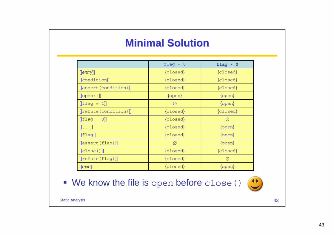
Minimal SolutionMinimal Solution

{open}{closed}[[exit]]

∅{closed}[[refute(flag)]]

{closed}{closed}[[close()]]

{open}∅[[assert(flag)]]

{open}{closed}[[flag]]

{open}{closed}[[...]]∅{closed}[[flag = 0]]

{closed}{closed}[[refute(condition)]]

{open}∅[[flag = 1]]

{open}{open}[[open()]]

{closed}{closed}[[assert(condition)]]

{closed}{closed}[[condition]]

{closed}{closed}[[entry]]

flag ≠ 0flag = 0

We know the file is open before close()

44

44Static Analysis

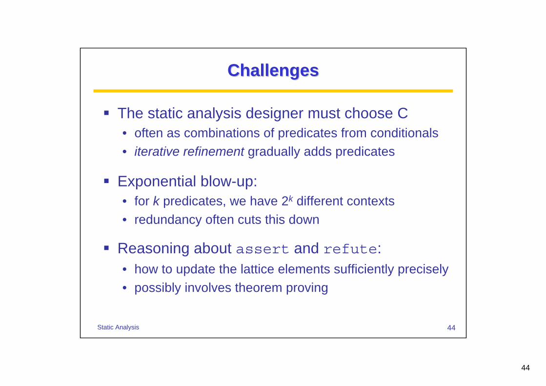
ChallengesChallenges

The static analysis designer must choose C• often as combinations of predicates from conditionals• iterative refinement gradually adds predicates

Exponential blow-up:• for k predicates, we have 2k different contexts• redundancy often cuts this down

Reasoning about assert and refute:• how to update the lattice elements sufficiently precisely• possibly involves theorem proving

45

45Static Analysis

ImprovementsImprovements

Run auxiliary analyses first, for example:• constant propagation• sign analysis

will help in handling flag assignments

Dead code propagation, change:[[open()]] = λc.{open}

into the still sound but more precise:[[open()]] = λc.if JOIN(v)(c)=∅ then ∅ else {open}

46

46Static Analysis

Interprocedural AnalysisInterprocedural Analysis

Analyzing the body of a single function:• intraprocedural analysis

Analyzing the whole program with function calls:• interprocedural analysis

The alternative is to:• analyze each function in isolation• be maximally pessimistic about results of function calls

47

47Static Analysis

CFG for Whole ProgramsCFG for Whole Programs

Construct a CFG for each functionThen glue them together to reflect function calls

Assume that all function calls are of the form:

id = f(E1, ..., En);

This can always be obtained by rewriting

48

48Static Analysis

Shadow VariablesShadow Variables

Introduce some extra variables in the program

For every function f the variable ret-f denoting its return valueFor every call site with index i a variable call-idenoting the computed valueFor every local or formal x and call site with index i a register save-i-xFor every formal x and every call site with index ia temporary variable temp-i-x

49

49Static Analysis

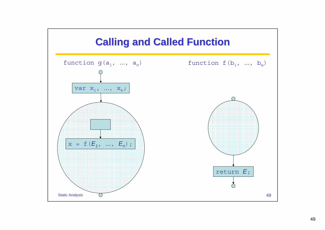
Calling and Called FunctionCalling and Called Function

x = f(E1, ..., En);

var x1, ..., xk;

return E;

function g(a1, ..., an) function f(b1, ..., bm)

50

50Static Analysis

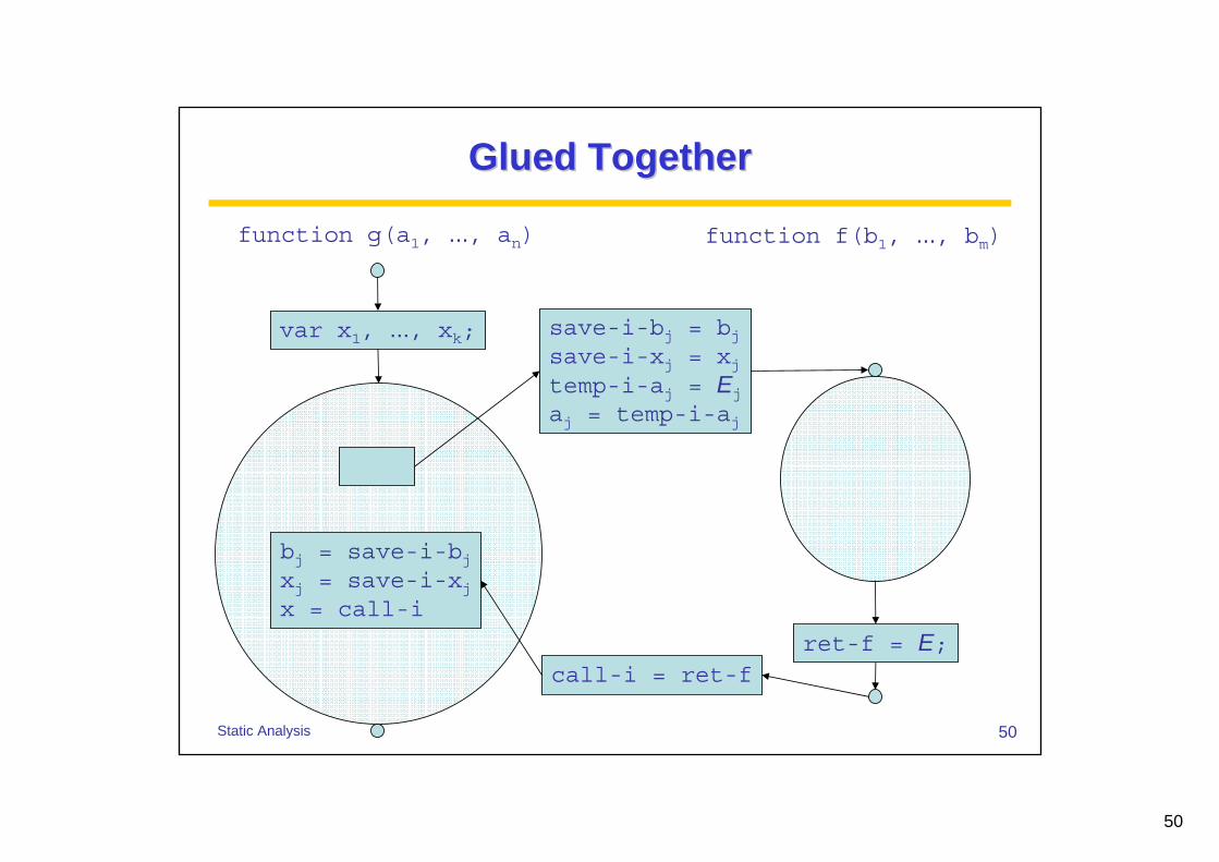
Glued TogetherGlued Together

bj = save-i-bjxj = save-i-xjx = call-i

var x1, ..., xk;

ret-f = E;

save-i-bj = bjsave-i-xj = xjtemp-i-aj = Ej

aj = temp-i-aj

call-i = ret-f

function g(a1, ..., an) function f(b1, ..., bm)

51

51Static Analysis

Example ProgramExample Program

foo(x,y) {

x = 2*y;

return x+1;

}

main() {

var a,b;

a = input;

b = foo(a,17);

return b;

}

52

52Static Analysis

Resulting CFGResulting CFG

foo(x,y) {

x = 2*y;

return x+1;

}

main() {

var a,b;

a = input;

b = foo(a,17);

return b;

}

var a,b

a = input

save-1-a = a

save-1-b = b

temp-1-x = a

temp-1-y = 17

x = temp-1-x

y = temp-1-y

x = 2*y

ret-foo = x+1

call-1 = ret-foo

a = save-1-a

b = save-1-b

b = call-1

ret-main = b

53

53Static Analysis

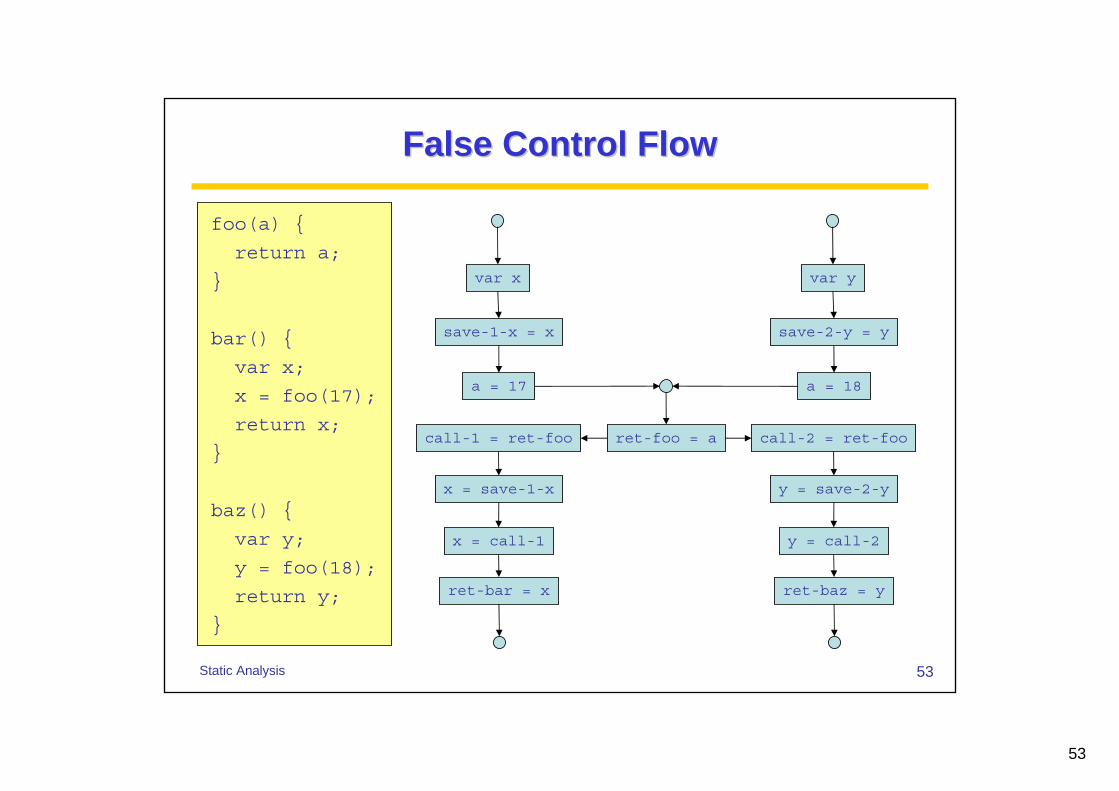
False Control FlowFalse Control Flow

foo(a) {

return a;

}

bar() {

var x;

x = foo(17);

return x;

}

baz() {

var y;

y = foo(18);

return y;

}

var x

save-1-x = x

a = 17

call-1 = ret-foo

x = save-1-x

x = call-1

ret-bar = x

var y

save-2-y = y

a = 18

call-2 = ret-foo

y = save-2-y

y = call-2

ret-baz = y

ret-foo = a

54

54Static Analysis

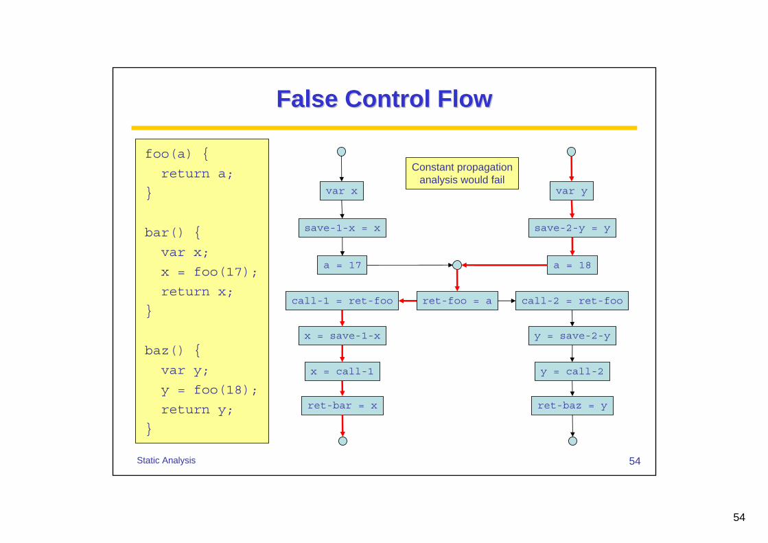
False Control FlowFalse Control Flow

foo(a) {

return a;

}

bar() {

var x;

x = foo(17);

return x;

}

baz() {

var y;

y = foo(18);

return y;

}

var x

save-1-x = x

a = 17

call-1 = ret-foo

x = save-1-x

x = call-1

ret-bar = x

var y

save-2-y = y

a = 18

call-2 = ret-foo

y = save-2-y

y = call-2

ret-baz = y

ret-foo = a

Constant propagationanalysis would fail

55

55Static Analysis

Polyvariance vs. MonovariancePolyvariance vs. Monovariance

A polyvariant analysis creates multiple copies of the CFG for the body of a called function

A monovariant analysis uses only one copy

Strategies determine the number of copies:• the simplest is one copy for each call site• dynamic heuristics are also possible• important that only finitely many copies are created

56

56Static Analysis

Polyvariant CFGPolyvariant CFG

var x

save-1-x = x

a = 17

call-1 = ret-foo

x = save-1-x

x = call-1

ret-bar = x

var y

save-2-y = y

a = 18

call-2 = ret-foo

y = save-2-y

y = call-2

ret-baz = y

ret-foo = a ret-foo = a

Constant propagationanalysis would succeed

57

57Static Analysis

Tree ShakingTree Shaking

Identify those functions that are never called• safely remove them from the program• reduces size of the compiled executable• reduces size of CFG for subsequent analyses

Uses monovariant interprocedural CFG

Essentially a transitive closure computation

58

58Static Analysis

Setting UpSetting Up

The lattice is the powerset of all function names

For every CFG node v we introduce a constraint variable [[v]] denoting the set of function that could possibly be called in the future

We let entry(id) denote the entry node in the CFG for the function named id

59

59Static Analysis

Tree Shaking ConstraintsTree Shaking Constraints

For assignments, conditions and output:[[v]] = [[w]] ∪ funcs(E) ∪ [[entry(f)]]

For all other nodes:[[v]] = [[w]]

Here funcs is defined as:• funcs(id) = funcs(intconst) = funcs(input) = ∅• funcs(E1 op E2) = funcs(E1) ∪ funcs(E2)• funcs(id(E1,...,En)) = {id} ∪ funcs(Ei)

∪w∈succ(v)

∪f∈funcs(E)

∪w∈succ(v)