data warehousing and olap. motivation aims of information technology: to help workers in their...

Data Warehousingand

OLAP

MotivationAims of information technology:

To help workers in their everyday business activity and improve their productivity – clerical data processing tasks

To help knowledge workers (executives, managers, analysts) make faster and better decisions – decision support systems

• Two types of applications:– Operational applications– Analytical applications

MotivationOn the other hand:

In most organizations, data about specific parts of business is there - lots and lots of data, somewhere, in some form.

Data is available but not information -- and not the right information at the right time.

Data warehouse is to: bring together information from multiple sources as to

provide a consistent database source for decision support queries.

off-load decision support applications from the on-line transaction system.

Warehousing• Growing industry: $ 8 billion in 1998• Range from desktop to huge warehouses

– Walmart: 900-CPU, 2,700 disks, 23TB– Teradata system

• Lots of new terms– ROLAP, MOLAP, HOLAP– rollup. drill-down, slice& dice

The Architecture of Data

Operational data

Metadata

Database schema

Summary data

Businessrules

What’s has been learned from data

Logical model

physical layout of data

who, what, when, where,

summaries by who, what, when, where,...

Decision Support and OLAP DSS: Information technology to help

knowledge workers (executives, managers, analysts) make faster and better decisions:

what were the sales volumes by region and by product category in the last year?

how did the share price of computer manufacturers correlate with quarterly profits over the past 10 years?

will a 10% discount increase sales volume sufficiently?

OLAP is an element of decision support system Data mining is a powerful, high-performance

data analysis tool for decision support.

Data Processing ModelsThere are two basic data processing models:

OLTP – the main aim of OLTP is reliable and efficient processing of a large number of transactions and ensuring data consistency.

OLAP – the main aim of OLAP is efficient multidimensional processing of large data volumes.

Traditional OLTPTraditionally, DBMS have been used for on-line transaction processing (OLTP)

order entry: pull up order xx-yy-zz and update status field

banking: transfer $100 from account X to account Y clerical data processing tasks detailed up-to-date data structured, repetitive tasks short transactions are the unit of work read and/or update a few records isolation, recovery, and integrity are critical

OLTP vs. OLAP• OLTP: On Line Transaction Processing

– Describes processing at operational sites• OLAP: On Line Analytical Processing

– Describes processing at warehouse

OLTP vs. OLAP OLTP OLAP

users Clerk, IT professional Knowledge workerfunction day to day operations decision supportDB design application-oriented subject-orienteddata current, up-to-date historical, summarized

detailed, flat relational multidimensional isolated integrated, consolidated

usage repetitive ad-hocaccess read/write, lots of scans

index/hash on prim. keyunit of work short, simple transaction complex query# records accessed tens millions#users thousandshundredsDB size 100MB-GB 100GB-TBmetric transaction throughput query throughput, response

What is a Data Warehouse “A data warehouse is a subject-oriented,

integrated, time-variant, and nonvolatile collection of data in support of management’s decision-making process.” --- W. H. Inmon

Collection of data that is used primarily in organizational decision making

A decision support database that is maintained separately from the organization’s operational database

Data Warehouse - Subject Oriented Subject oriented: oriented to the major

subject areas of the corporation that have been defined in the data model. E.g. for an insurance company: customer,

product, transaction or activity, policy, claim, account, and etc.

Operational DB and applications may be organized differently E.g. based on type of insurance's: auto, life,

medical, fire, ...

Data Warehouse – Integrated

There is no consistency in encoding, naming conventions, …, among different data sources

Heterogeneous data sources When data is moved to the warehouse, it is

converted.

Data Warehouse - Non-Volatile

Operational data is regularly accessed and manipulated a record at a time, and update is done to data in the operational environment.

Warehouse Data is loaded and accessed. Update of data does not occur in the data warehouse environment.

Data Warehouse - Time Variance The time horizon for the data warehouse is

significantly longer than that of operational systems.

Operational database: current value data. Data warehouse data : nothing more than a

sophisticated series of snapshots, taken of at some moment in time.

The key structure of operational data may or may not contain some element of time. The key structure of the data warehouse always contains some element of time.

Why Separate Data Warehouse?

Performance special data organization, access methods, and

implementation methods are needed to support multidimensional views and operations typical of OLAP

Complex OLAP queries would degrade performance for operational transactions

Concurrency control and recovery modes of OLTP are not compatible with OLAP analysis

Why Separate Data Warehouse? Function

missing data: Decision support requires historical data which operational DBs do not typically maintain

data consolidation: DS requires consolidation (aggregation, summarization) of data from heterogeneous sources: operational DBs, external sources

data quality: different sources typically use inconsistent data representations, codes and formats which have to be reconciled.

Advantages of Warehousing

• High query performance• Queries not visible outside warehouse• Local processing at sources unaffected• Can operate when sources unavailable• Can query data not stored in a DBMS• Extra information at warehouse

– Modify, summarize (store aggregates)– Add historical information

Advantages of Mediator Systems

• No need to copy data– less storage– no need to purchase data

• More up-to-date data• Query needs can be unknown• Only query interface needed at sources• May be less draining on sources

ExtractTransformLoadRefresh

Data Warehouse

Metadatarepository

Data martsServes

OLAPserver

OLAP Data miningReports

Operational databases

External datasources

The Architecture of Data Warehousing

Data Sources Data sources are often the operational systems,

providing the lowest level of data. Data sources are designed for operational use, not

for decision support, and the data reflect this fact. Multiple data sources are often from different

systems, run on a wide range of hardware and much of the software is built in-house or highly customized.

Multiple data sources introduce a large number of issues -- semantic conflicts.

Creating and Maintaining a Warehouse

Data warehouse needs several tools that automate or support tasks such as:

Data extraction from different external data sources, operational databases, files of standard applications (e.g. Excel, COBOL applications), and other documents (Word, WWW).

Data cleaning (finding and resolving inconsistency in the source data)

Integration and transformation of data (between different data formats, languages, etc.)

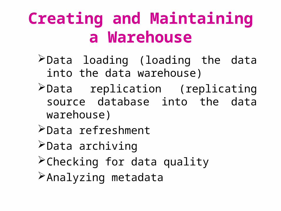
Creating and Maintaining a Warehouse

Data loading (loading the data into the data warehouse)

Data replication (replicating source database into the data warehouse)

Data refreshmentData archivingChecking for data qualityAnalyzing metadata

Physical Structure of Data Warehouse

There are three basic architectures for constructing a data warehouse:

Centralized Distributed Federated Tiered

The data warehouse is distributed for: load balancing, scalability and higher availability


CentralData

Warehouse

Client Client Client

Source Source

Centralized architecture


LogicalData

Warehouse

Source Source

LocalData Marts

EndUsers

MarketingFinancialDistribution

Federated architecture


PhysicalData

Warehouse

LocalData Marts

Workstations(higly summarizeddata)

Source Source

Tiered architecture


• Federated architecture– The logical data warehouse is only virtual

• Tiered architecture The central data warehouse is physical There exist local data marts on different tiers

which store copies or summarization of the previous tier.

Conceptual Modeling ofData Warehouses

Three basic conceptual schemas:

• Star schema• Snowflake schema• Fact constellations

Star schema

Star schema: A single object (fact table) in the middle connected to a number of dimension tables

Star schema

saleorderId

datecustIdprodIdstoreId

qtyamt

customercustIdname

addresscity

productprodIdnameprice

storestoreId

city

Star schema

customer custId name address city53 joe 10 main sfo81 fred 12 main sfo

111 sally 80 willow la

product prodId name pricep1 bolt 10p2 nut 5

store storeId cityc1 nycc2 sfoc3 la

sale oderId date custId prodId storeId qty amto100 1/7/97 53 p1 c1 1 12o102 2/7/97 53 p2 c1 2 11o105 3/8/97 111 p1 c3 5 50

Terms Basic notion: a measure (e.g. sales, qty,

etc) Given a collection of numeric measures

Each measure depends on a set of dimensions (e.g. sales volume as a function of product, time, and location)

Terms

• Relation, which relates the dimensions to the measure of interest, is called the fact table (e.g. sale)

• Information about dimensions can be represented as a collection of relations – called the dimension tables (product, customer, store)

• Each dimension can have a set of associated attributes

DateMonthYear

Date

CustIdCustNameCustCityCustCountry

Customer

Sales Fact Table

Date

Product

Store

Customer

unit_sales

dollar_sales

schilling_sales

Measurements

ProductNoProdNameProdDescCategoryQOH

Product

StoreIDCityStateCountryRegion

Store

Example of Star Schema

Dimension Hierarchies• For each dimension, the set of associated

attributes can be structured as a hierarchy

storesType

city region

customer city state country

Dimension Hierarchies

store storeId cityId tId mgrs5 sfo t1 joes7 sfo t2 freds9 la t1 nancy

city cityId pop regIdsfo 1M northla 5M south

region regId namenorth cold regionsouth warm region

sType tId size locationt1 small downtownt2 large suburbs

Snowflake Schema

Snowflake schema: A refinement of star schema where the dimensional hierarchy is represented explicitly by normalizing the dimension tables

Sales Fact Table Date

Product

Store

Customer

unit_sales

dollar_sales

schilling_sales

ProductNoProdNameProdDescCategoryQOH

Product

CustIdCustNameCustCityCustCountry

Cust

DateMonth

DateMonthYear

MonthYear

Year

CityState

City

CountryRegion

Country

StateCountry

State

StoreIDCity

Store

Measurements

Example of Snowflake Schema

Fact constellations

Fact constellations: Multiple fact tables share dimension tables

Database design methodology for data warehouses (1)

• Nine-step methodology – proposed by KimballStep Activity

1 Choosing the process2 Choosing the grain3 Identifying and conforming the dimensions4 Choosing the facts5 Storing the precalculations in the fact table6 Rounding out the dimension tables7 Choosing the duration of the database8 Tracking slowly changing dimensions9 Deciding the query priorities and the query modes

Database design methodology for data warehouses (2)

• There are many approaches that offer alternative routes to the creation of a data warehouse

• Typical approach – decompose the design of the data warehouse into manageable parts – data marts, At a later stage, the integration of the smaller data marts leads to the creation of the enterprise-wide data warehouse.

• The methodology specifies the steps required for the design of a data mart, however, the methodology also ties together separate data marts so that over time they merge together into a coherent overall data warehouse.

Step 1: Choosing the process

• The process (function) refers to the subject matter of a particular data marts. The first data mart to be built should be the one that is most likely to be delivered on time, within budget, and to answer the most commercially important business questions.

• The best choice for the first data mart tends to be the one that is related to ‘sales’

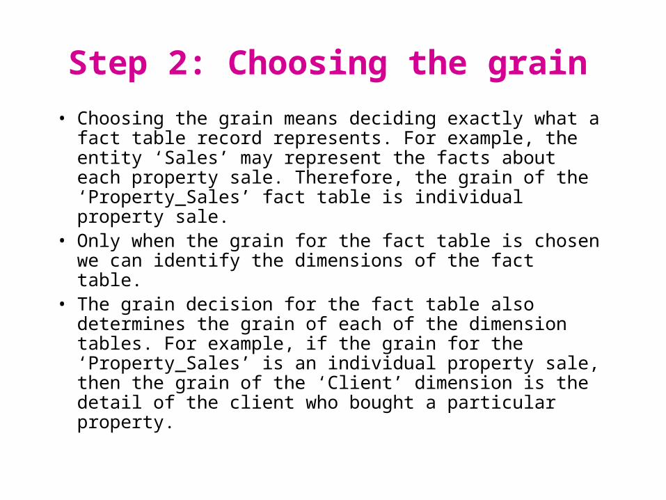
Step 2: Choosing the grain• Choosing the grain means deciding exactly what a fact

table record represents. For example, the entity ‘Sales’ may represent the facts about each property sale. Therefore, the grain of the ‘Property_Sales’ fact table is individual property sale.

• Only when the grain for the fact table is chosen we can identify the dimensions of the fact table.

• The grain decision for the fact table also determines the grain of each of the dimension tables. For example, if the grain for the ‘Property_Sales’ is an individual property sale, then the grain of the ‘Client’ dimension is the detail of the client who bought a particular property.

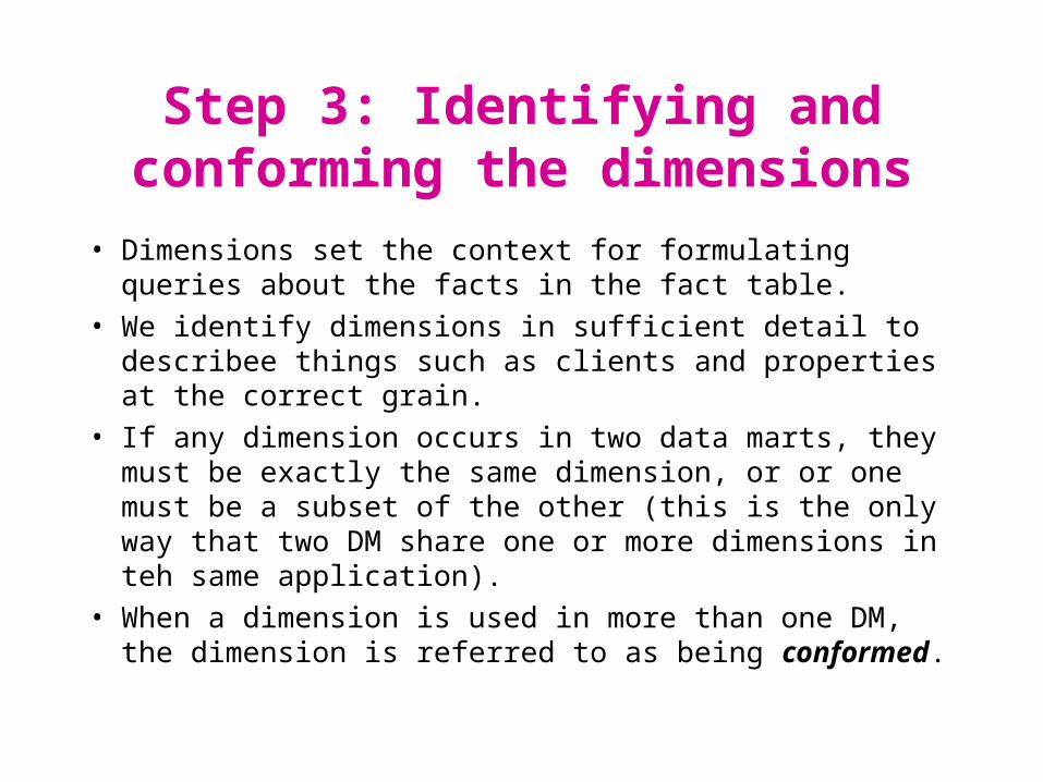
Step 3: Identifying and conforming the dimensions

• Dimensions set the context for formulating queries about the facts in the fact table.

• We identify dimensions in sufficient detail to describee things such as clients and properties at the correct grain.

• If any dimension occurs in two data marts, they must be exactly the same dimension, or or one must be a subset of the other (this is the only way that two DM share one or more dimensions in teh same application).

• When a dimension is used in more than one DM, the dimension is referred to as being conformed.

Step 4: Choosing the facts

• The grain of the fact table determines which facts can be used in the data mart – all facts must be expressed at the level implied by the grain.

• In other words, if the grain of the fact table is an individual property sale, then all the numerical facts must refer to this particular sale (the facts should be numeric and additive).

Step 5: Storing pre-calculations in the fact table

• Once the facts have been selected each should be re-examined to determine whether there are opportunities to use pre-calculations.

• Common example: a profit or loss statement• These types of facts are useful since they are additive

quantities, from which we can derive valuable information.• This is particularly true for a value that is fundamental to

an enterprise, or if there is any chance of a user calculating the value incorrectly.

Step 6: Rounding out the dimension tables

• In this step we return to the dimension tables and add as many text descriptions to the dimensions as possible.

• The text descriptions should be as intuitive and understandable to the users as possible

Step 7: Choosing the duration of the data warehouse

• The duration measures how far back in time the fact table goes.

• For some companies (e.g. insurance companies) there may be a legal requirement to retain data extending back five or more years.

• Very large fact tables raise at least two very significant data warehouse design issues:– The older data, the more likely there will be problems in reading

and interpreting the old files– It is mandatory that the old versions of the important dimensions

be used, not the most current versions (we will discuss this issue later on)

Step 8: Tracking slowly changing dimensions

• The changing dimension problem means that the proper description of the old client and the old branch must be used with the old data warehouse schema

• Usually, the data warehouse must assign a generalized key to these important dimensions in order to distinguish multiple snapshots of clients and branches over a period of time

• There are different types of changes in dimensions:– A dimension attribute is overwritten– A dimension attribute caauses a new dimension record to be created– etc.

Step 9: Deciding the query priorities and the query modes

• In this step we consider physical design issues. – The presence of pre-stored summaries and aggregates– Indices– Materialized views– Security issue– Backup issue– Archive issue

Database design methodology for data warehouses - summary

• At the end of this methodology, we have a design for a data mart that supports the requirements of a particular bussiness process and allows the easy integration with other related data martsto ultimately form the enterprise-wide data warehouse.

• A dimensional model, which contains more than one fact table sharing one or more conformed dimension tables, is referred to as a fact constellation.

Multidimensional Data Model

Sales of products may be represented in one dimension (as a fact relation) or in two dimensions, e.g. : clients and products



sale Product Client Amtp1 c1 12p2 c1 11p1 c3 50p2 c2 8

c1 c2 c3p1 12 50p2 11 8

Fact relation Two-dimensional cube


sale Product Client Date Amtp1 c1 1 12p2 c1 1 11p1 c3 1 50p2 c2 1 8p1 c1 2 44p1 c2 2 4

day 2 c1 c2 c3p1 44 4p2 c1 c2 c3

p1 12 50p2 11 8

day 1

Fact relation 3-dimensional cube

Multidimensional Data Model and Aggregates

• Add up amounts for day 1• In SQL: SELECT sum(Amt) FROM SALE

WHERE Date = 1


81result


• Add up amounts by day• In SQL: SELECT Date, sum(Amt)

FROM SALE GROUP BY Date


Date sum1 812 48

result


• Add up amounts by client, product• In SQL: SELECT client, product, sum(amt)

FROM SALE GROUP BY client, product



sale Product Client Sump1 c1 56p1 c2 4

p1 c3 50 p2 c1 11

p2 c2 8


• In multidimensional data model together with measure values usually we store summarizing information (aggregates)

c1 c2 c3 Sump1 56 4 50 110p2 11 8 19

Sum 67 12 50 129

Aggregates• Operators: sum, count, max, min,

median, ave• “Having” clause• Using dimension hierarchy

– average by region (within store)– maximum by month (within date)

Cube Aggregation

day 2 c1 c2 c3p1 44 4p2 c1 c2 c3

p1 12 50p2 11 8

c1 c2 c3p1 56 4 50p2 11 8

c1 c2 c3sum 67 12 50

sump1 110p2 19

129

. . .Example: computing sums

day 1

Cube Operators

day 2 c1 c2 c3p1 44 4p2 c1 c2 c3

p1 12 50p2 11 8

c1 c2 c3p1 56 4 50p2 11 8

c1 c2 c3sum 67 12 50

sump1 110p2 19

129

. . .

sale(c1,*,*)

sale(*,*,*)sale(c2,p2,*)

day 1

Cube

c1 c2 c3 *p1 56 4 50 110p2 11 8 19* 67 12 50 129day 2 c1 c2 c3 *

p1 44 4 48p2* 44 4 48

c1 c2 c3 *p1 12 50 62p2 11 8 19* 23 8 50 81

day 1

*

sale(*,p2,*)

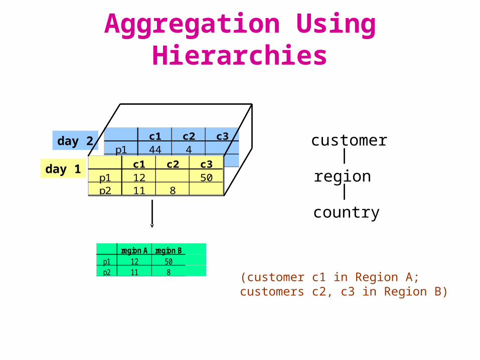
Aggregation Using Hierarchies

day 2 c1 c2 c3p1 44 4p2 c1 c2 c3

p1 12 50p2 11 8

day 1

region A region Bp1 12 50p2 11 8

customer

region

country

(customer c1 in Region A;customers c2, c3 in Region B)

Aggregation Using Hierarchies

c1c2

c3c4

videoCamera

New Orleans

Poznań

CD

Date of sale

10121112

35

711

219715

Video Camera CDNO 22 8 30PN 23 18 22

aggregation withrespect to city

client

city

region

A Sample Data Cube

sum

sum

sum

USA

Canada

Mexico

Country

Date

Product

CDvideocamera

1Q 2Q 3Q 4Q

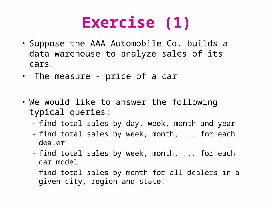
Exercise (1)• Suppose the AAA Automobile Co. builds a data

warehouse to analyze sales of its cars. • The measure - price of a car

• We would like to answer the following typical queries:– find total sales by day, week, month and year– find total sales by week, month, ... for each dealer– find total sales by week, month, ... for each car model– find total sales by month for all dealers in a given city,

region and state.

Exercise (2)• Dimensions:

– time (day, week, month, quarter, year)– dealer (name, city, state, region, phone)– cars (serialno, model, color, category , …)

• Design the conceptual data warehouse schema

OLAP Servers Relational OLAP (ROLAP):

Extended relational DBMS that maps operations on multidimensional data to standard relations operations

Store all information, including fact tables, as relations

Multidimensional OLAP (MOLAP): Special purpose server that directly

implements multidimensional data and operations

store multidimensional datasets as arrays

OLAP Servers

Hybrid OLAP (HOLAP): Give users/system administrators freedom to

select different partitions.

OLAP Queries Roll up: summarize data along a

dimension hierarchy if we are given total sales volume per city we

can aggregate on the Location to obtain sales per states

OLAP Queries

c1c2

c3c4

videoCamera

New Orleans

Poznań

CD

Date of sale

10121112

35

711

219715

Video Camera CDNO 22 8 30PN 23 18 22

city

region

client

roll up

OLAP Queries

Roll down, drill down: go from higher level summary to lower level summary or detailed data For a particular product category, find the

detailed sales data for each salesperson by date

Given total sales by state, we can ask for sales per city, or just sales by city for a selected state

OLAP Queries

day 2 c1 c2 c3p1 44 4p2 c1 c2 c3

p1 12 50p2 11 8

c1 c2 c3p1 56 4 50p2 11 8

c1 c2 c3sum 67 12 50

sump1 110p2 19

129

drill-down

rollup

day 1

OLAP Queries• Slice and dice: select and project

Sales of video in USA over the last 6 months Slicing and dicing reduce the number of

dimensions Pivot: reorient cube

The result of pivoting is called a cross-tabulation

If we pivot the Sales cube on the Client and Product dimensions, we obtain a table for each client for each product value

OLAP Queries Pivoting can be combined with aggregation

sale prodId clientid date amtp1 c1 1 12p2 c1 1 11p1 c3 1 50p2 c2 1 8p1 c1 2 44p1 c2 2 4

day 2 c1 c2 c3p1 44 4p2 c1 c2 c3

p1 12 50p2 11 8

day 1

c1 c2 c3 Sump1 56 4 50 110p2 11 8 19

Sum 67 12 50 129

c1 c2 c3 Sum1 23 8 50 812 44 4 48

Sum 67 12 50 129

OLAP Queries Ranking: selection of first n elements (e.g. select 5

best purchased products in July) Others: stored procedures, selection, etc.• Time functions

– e.g., time average

Implementing a Warehouse


• Designing and rolling out a data warehouse is a complex process, consisting of the following activities: Define the architecture, do capacity palnning,

and select the storage servers, database and OLAP servers (ROLAP vs MOLAP), and tools,

Integrate the servers, storage, and client tools, Design the warehouse schema and views,


Define the physical warehouse organization, data placement, partitioning, and access method,

Connect the sources using gateways, ODBC drivers, or other wrappers,

Design and implement scripts for data extraction, cleaning, transformation, load, and refresh,

Implementing a Warehouse Populate the repository with the schema and

view definitions, scripts, and other metadata, Design and implement end-user applications, Roll out the warehouse and applications.


• Monitoring: Sending data from sources• Integrating: Loading, cleansing,...• Processing: Query processing, indexing, ...• Managing: Metadata, Design, ...

Monitoring

• Data Extraction– Data extraction from external sources is usually

implemented via gateways and standard interfaces (such as Information Builders EDA/SQL, ODBC, JDBC, Oracle Open Connect, Sybase Enterprise Connect, Informix Enterprise Gateway, etc.)

Monitoring Techniques Detect changes to an information source

that are of interest to the warehouse: define triggers in a full-functionality DBMS examine the updates in the log file write programs for legacy systems polling (queries to source) screen scraping

Propagate the change in a generic form to the integrator

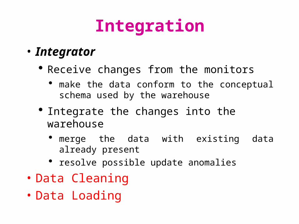
Integration• Integrator

Receive changes from the monitors make the data conform to the conceptual schema

used by the warehouse

Integrate the changes into the warehouse merge the data with existing data already present resolve possible update anomalies

• Data Cleaning• Data Loading

Data Cleaning

• Data cleaning is important to warehouse – there is high probability of errors and anomalies in the data: – inconsistent field lengths, inconsistent

descriptions, inconsistent value assignments, missing entries and violation of integrity constraints.

– optional fields in data entry are significant sources of inconsistent data.

Data Cleaning Techniques Data migration: allows simple data

transformation rules to be specified, e.g. „replace the string gender by sex” (Warehouse Manager from Prism is an example of this tool)

Data scrubbing: uses domain-specific knowledge to scrub data (e.g. postal addresses) (Integrity and Trillum fall in this category)

Data auditing: discovers rules and relationships by scanning data (detect outliers). Such tools may be considered as variants of data mining tools

Data Loading• After extracting, cleaning and transforming, data

must be loaded into the warehouse. • Loading the warehouse includes some other

processing tasks: checking integrity constraints, sorting, summarizing, etc.

• Typically, batch load utilities are used for loading. A load utility must allow the administrator to monitor status, to cancel, suspend, and resume a load, and to restart after failure with no loss of data integrity

Data Loading Issues

• The load utilities for data warehouses have to deal with very large data volumes

• Sequential loads can take a very long time.• Full load can be treated as a single long batch

transaction that builds up a new database. Using checkpoints ensures that if a failure occurs during the load, the process can restart from the last checkpoint

Data Refresh• Refreshing a warehouse means propagating

updates on source data to the data stored in the warehouse

when to refresh: periodically (daily or weekly) immediately (defered refresh and immediate

refresh)– determined by usage, types of data source, etc.

Data Refresh how to refresh

– data shipping– transaction shipping

• Most commercial DBMS provide replication servers that support incremental techniques for propagating updates from a primary database to one or more replicas. Such replication servers can be used to incrementally refresh a warehouse when sources change

Data Shipping

• data shipping: (e.g. Oracle Replication Server), a table in the warehouse is treated as a remote snapshot of a table in the source database. After_row trigger is used to update snapshot log table and propagate the updated data to the warehouse

Transaction Shipping

• transaction shipping: (e.g. Sybase Replication Server, Microsoft SQL Server), the regular transaction log is used. The transaction log is checked to detect updates on replicated tables, and those log records are transferred to a replication server, which packages up the corresponding transactions to update the replicas

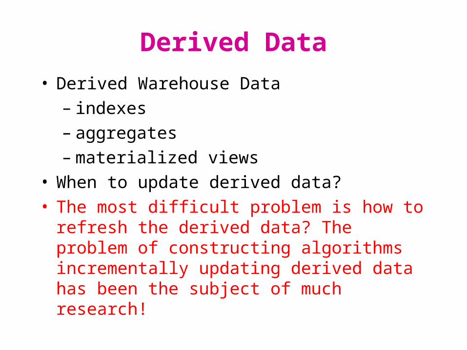
Derived Data• Derived Warehouse Data

– indexes– aggregates– materialized views

• When to update derived data?• The most difficult problem is how to refresh the

derived data? The problem of constructing algorithms incrementally updating derived data has been the subject of much research!

Materialized Views• Define new warehouse relations using SQL

expressionssale prodId clientid date amt

p1 c1 1 12p2 c1 1 11p1 c3 1 50p2 c2 1 8p1 c1 2 44p1 c2 2 4

product id name pricep1 bolt 10p2 nut 5

joinTb prodId name price clientid date amtp1 bolt 10 c1 1 12p2 nut 5 c1 1 11p1 bolt 10 c3 1 50p2 nut 5 c2 1 8p1 bolt 10 c1 2 44p1 bolt 10 c2 2 4

join of sale and product

Processing• Index Structures• What to Materialize?• Algorithms

Index Structures• Indexing principle:

mapping key values to records for associative direct access

Most popular indexing techniques in relational database: B+-trees

For multi-dimensional data, a large number of indexing techniques have been developed: R-trees

Index Structures• Index structures applied in warehouses

– inverted lists– bit map indexes– join indexes– text indexes

Inverted Lists

2023

1819

202122

232526

r4r18r34r35

r5r19r37r40

rId name ager4 joe 20

r18 fred 20r19 sally 21r34 nancy 20r35 tom 20r36 pat 25r5 dave 21

r41 jeff 26

. . .

ageindex

invertedlists

datarecords

Inverted Lists

• Query: – Get people with age = 20 and name = “fred”

• List for age = 20: r4, r18, r34, r35• List for name = “fred”: r18, r52• Answer is intersection: r18

Bitmap Indexes• Bitmap index: An indexing technique that has

attracted attention in multi-dimensional database implementationtable

Customer City Carc1 Detroit Fordc2 Chicago Hondac3 Detroit Hondac4 Poznan Fordc5 Paris BMWc6 Paris Nissan

Bitmap Indexes• The index consists of bitmaps:

Index on City:ec1 Chicago Detroit Paris Poznan

1 0 1 0 02 1 0 0 03 0 1 0 04 0 0 0 15 0 0 1 06 0 0 1 0

bitmaps

Bitmap IndexesIndex on Car:

ec1 BMW Ford Honda Nissan1 0 1 0 02 1 0 1 03 0 0 1 04 0 1 0 05 1 0 0 06 0 0 0 1

bitmaps

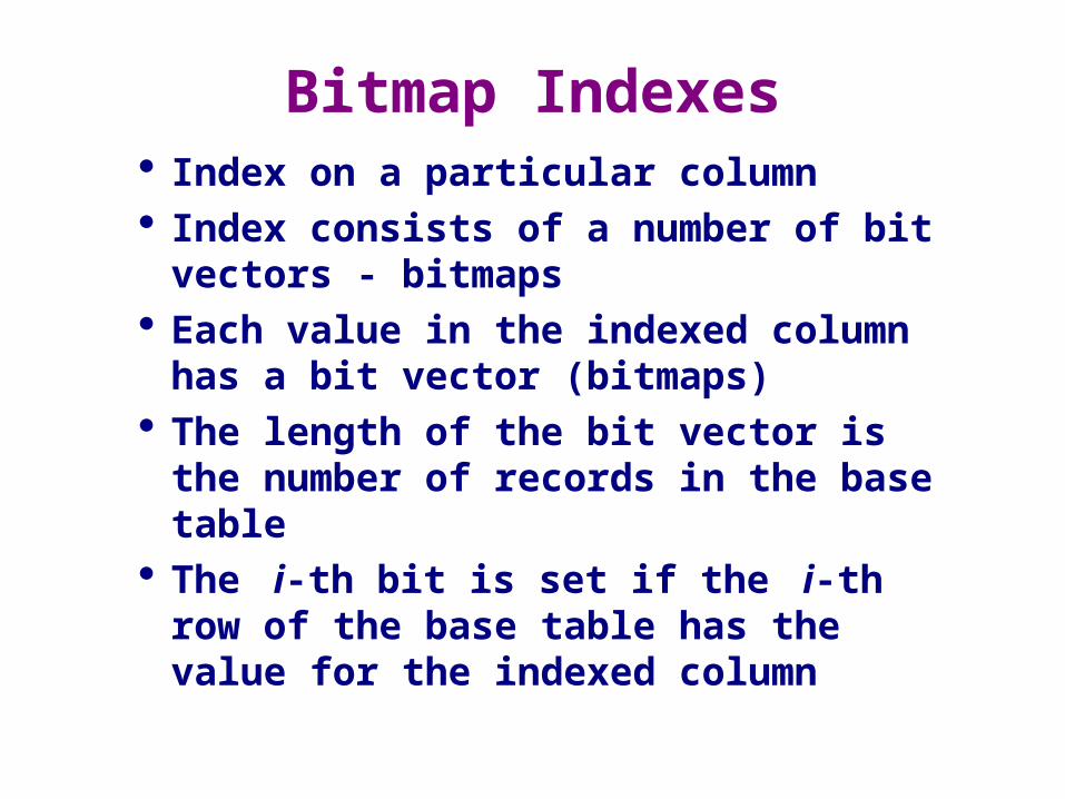
Bitmap Indexes Index on a particular column Index consists of a number of bit vectors -

bitmaps Each value in the indexed column has a bit

vector (bitmaps) The length of the bit vector is the number of

records in the base table The i-th bit is set if the i-th row of the base

table has the value for the indexed column

Bitmap Index

2023

1819

202122

232526

id name age1 joe 202 fred 203 sally 214 nancy 205 tom 206 pat 257 dave 218 jeff 26

. . .

ageindex

bitmaps

datarecords

110110000

0010001011

Using Bitmap indexes• Query:

– Get people with age = 20 and name = “fred”• List for age = 20: 1101100000• List for name = “fred”: 0100000001• Answer is intersection: 010000000000 Good if domain cardinality small Bit vectors can be compressed

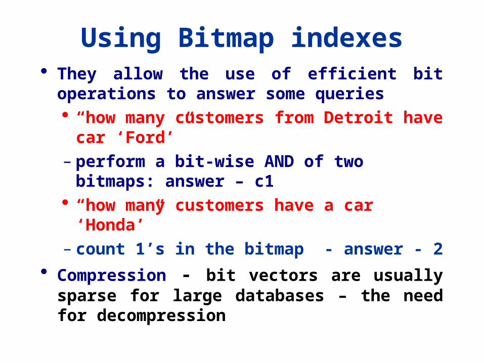
Using Bitmap indexes They allow the use of efficient bit operations to

answer some queries “how many customers from Detroit have car

‘Ford’”– perform a bit-wise AND of two bitmaps:

answer – c1 “how many customers have a car ‘Honda’”– count 1’s in the bitmap - answer - 2

Compression - bit vectors are usually sparse for large databases – the need for decompression

Bitmap Index – Summary With efficient hardware support for bitmap

operations (AND, OR, XOR, NOT), bitmap index offers better access methods for certain queries

e.g., selection on two attributes Some commercial products have implemented

bitmap index Works poorly for high cardinality domains since

the number of bitmaps increases Difficult to maintain - need reorganization when

relation sizes change (new bitmaps)

Join• “Combine” SALE, PRODUCT relations• In SQL: SELECT * FROM SALE, PRODUCT

sale prodId storeId date amtp1 c1 1 12p2 c1 1 11p1 c3 1 50p2 c2 1 8p1 c1 2 44p1 c2 2 4

product id name pricep1 bolt 10p2 nut 5

joinTb prodId name price storeId date amtp1 bolt 10 c1 1 12p2 nut 5 c1 1 11p1 bolt 10 c3 1 50p2 nut 5 c2 1 8p1 bolt 10 c1 2 44p1 bolt 10 c2 2 4

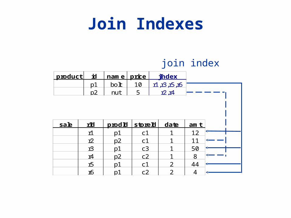
Join Indexes

product id name price jIndexp1 bolt 10 r1,r3,r5,r6p2 nut 5 r2,r4

sale rId prodId storeId date amtr1 p1 c1 1 12r2 p2 c1 1 11r3 p1 c3 1 50r4 p2 c2 1 8r5 p1 c1 2 44r6 p1 c2 2 4

join index

Join Indexes Traditional indexes map the value to a list of

record ids. Join indexes map the tuples in the join result of two relations to the source tables.

In data warehouse cases, join indexes relate the values of the dimensions of a star schema to rows in the fact table. For a warehouse with a Sales fact table and dimension

city, a join index on city maintains for each distinct city a list of RIDs of the tuples recording the sales in the city

Join indexes can span multiple dimensions

What to Materialize?• Store in warehouse results useful for

common queriesExample:

day 2 c1 c2 c3p1 44 4p2 c1 c2 c3

p1 12 50p2 11 8

day 1

c1 c2 c3p1 56 4 50p2 11 8

c1 c2 c3p1 67 12 50

c1p1 110p2 19

129

. . .

materialize

total sale

Cube Operation• SELECT date, product, customer, SUM

(amount)

FROM SALES

CUBE BY date, product, customer• Need compute the following Group-Bys

– (date, product, customer),– (date,product),(date, customer), (product,

customer),– (date), (product), (customer)

Cuboid Lattice Data cube can be viewed as a lattice of

cuboids The bottom-most cuboid is the base cube. The top most cuboid contains only one cell.

(B)(A) (C) (D)

(B,C) (B,D) (C,D)(A,D)(A,C)

(A,B,D) (B,C,D)(A,C,D)

(A,B)

( all )

(A,B,C,D)

(A,B,C)

Cuboid Lattice

city, product, date

city, product city, date product, date

city product date

all

day 2 c1 c2 c3p1 44 4p2 c1 c2 c3

p1 12 50p2 11 8

day 1

c1 c2 c3p1 56 4 50p2 11 8

c1 c2 c3p1 67 12 50

129

use greedyalgorithm todecide whatto materialize

Efficient Data Cube Computation

Materialization of data cube Materialize every (cuboid), none, or some. Algorithms for selection of which cuboids to

materialize:• size, sharing, and access frequency:

– Type/frequency of queries– Query response time– Storage cost– Update cost

Dimension Hierarchies • Client hierarchy

region

state

city

cities city state regionc1 CA Eastc2 NY Eastc3 SF West

Dimension Hierarchies Computation

city, product

city, product, date

city, date product, date

city product date

all

state, product, date

state, date

state, product

state

roll-up along clienthierarchy

Cube Computation - Array Based Algorithm

An MOLAP approach: the base cuboid is stored as

multidimensional array. read in a number of cells to compute partial

cuboids

Cube computations

A

C

{ABC}{AB}{AC}{BC}{A}{B}{C}{ }

B

ALL

View and Materialized Views View

derived relation defined in terms of base (stored) relations

Materialized views a view can be materialized by storing the tuples

of the view in the database index structures can be built on the materialized

view

View and Materialized Views

Maintenance is an issue for materialized views

recomputation incremental updating

Maintenance of materialized views• “Deficit” departments• To find all “deficit” departments:

– group by deptid– join (deptid)– select all dept.names with budget < sum(salary)

DeptId Name Budget1 CS 75002 Math 55003 Comm. 4500

EmpId Lname salary DeptId100 Kim 2500 1200 Jabbar 2000 1300 Smith 3000 1400 Brown 3500 2500 Lu 3000 2

Maintenance of materialized views• select DeptId, sum(salary) Real_Budget

from Employeegroup by DeptId; Temp (relation)

• select Namefrom Dept, Tempwhere Dept.DeptId=Temp.DeptIdand Budget < Real_Budget;

Maintenance of materialized views

• assume the following update:update Employeeset salary=salary+1000

where Lname=‘Jabbar’;• recompute the whole view?• use intermediate materialized results

(Temp), and update the view incrementally?

Managing

Metadata Repository

Administrative metadata source database and their contents gateway descriptions warehouse schema, view and derived data

definitions dimensions and hierarchies pre-defined queries and reports data mart locations and contents

Metadata Repository

Administrative metadata data partitions data extraction, cleansing, transformation rules,

defaults data refresh and purge rules user profiles, user groups security: user authorization, access control

Metadata Repository• Business

– business terms & definition– data ownership, charging

• Operational– data layout– data currency (e.g., active, archived, purged)– use statistics, error reports, audit trails

Design• What data is needed?• Where does it come from?• How to clean data?• How to represent in warehouse (schema)?• What to summarize?• What to materialize?• What to index?

Summary Data warehouse is not a software product

or application - it is an important information processing system architecture for decision making!

Data warehouse combines a number of products, each has operational uses besides data warehouse

Summary OLAP provides powerful and fast tools

for reporting on data: ROLAP vs. MOLAP

Issues associated with data warehouses: new techniques: multidimensional database,

data cube computation, query optimization, indexing, …

data warehousing and application design: vendors and application developers.

Current State of Industry• Extraction and integration done off-line

– Usually in large, time-consuming, batches• Everything copied at warehouse

– Not selective about what is stored– Query benefit vs storage & update cost

• Query optimization aimed at OLTP– High throughput instead of fast response– Process whole query before displaying anything

Research• Incremental Maintenance• Data Consistency• Data Expiration• Recovery• Data Quality• Dynamic Data Warehouses (how to

maintain data warehouse over changing external data sources?)

Research• Rapid Monitor Construction• Materialization & Index Selection• Data Fusion• Integration of Text & Relational Data &

Semistructured Data & …..• Data Mining

data warehousing and olap. motivation aims of information technology: to help workers in their...

Documents