Data visualizationVisual perception and encoding

David Hoksza

http://siret.cz/hoksza

Course outline

• Visual perception, design principles

• Tables and charts visualization

• Web-based visualization, D3.js

2

• Dimension reduction

• Networks-like data visualization

• (Infographics)

• Project presentations

Design and programming

Algorithms

“Soft skills”

Course organization

Classes

• Once per two weeks

• Practical visualization• Tableau, D3.js, …

• Projects• Presentation at the end of the

semester

Examination

• Oral exam

Classification

• Examination (60%)

• Project (40%)

Projects

• Slides for presentation

• Problem walkthrough

• Data format description

• Code description• Components used

• Problematic points

• Interesting points

• Conclusion

4

Lecture outline

• Motivation

• Visual perception

• Visual encoding

• Data types and relations

• Measures

5

Data science process

Computer science

• Acquire

• Parse

• data wrangling (munging)

Statistics and data mining

• Filter

• Mine

Graphics design

• Represent

• Refine

InfoVis and HCI

• Interact

6

Basically ETL (Extraction,

Transformation, Loading)

known from data

warehousing

Core of data science –

Exploratory Data

Analysis (EDA)

Visual encoding of the

numerical data

Ways to let user interact

with the data to get new

insights

Goals of data visualization

• To communicate information clearly and effectively through graphical means

• To help find the desired information more effectively and intuitively• Picking up things with the naked eye that would otherwise be hidden

• To explore patterns in the data

• Data usually has a structure which needs to be revealed using data visualization

• Turning numbers into story → storytelling with data

7

Exploratory vs explanatory visualization

Exploratory visualization

• What the data is, what is hidden in the data

• Enables users to look at the data from different angles

Explanatory visualization

• Helping a user to make sense of the data by choosing the right visualization techniques

• Need to know the context from which the audience come and what they need to know

• Strategic placements of elements and choice of attributes to communicate the information clearly and help users to focus on what is important

8

You and

data

Data and your

audience

Graphics over statistics

Four data sets with nearly identical linear

model (mean, variance, linear regression

line, correlation coefficient)

• Visualization can reveal/distinguish data/trends/patterns, … which statistics can not

Anscombe’s quartet

I II III IV

x y x y x y x y

10.0 8.04 10.0 9.14 10.0 7.46 8.0 6.58

8.0 6.95 8.0 8.14 8.0 6.77 8.0 5.76

13.0 7.58 13.0 8.74 13.0 12.74 8.0 7.71

9.0 8.81 9.0 8.77 9.0 7.11 8.0 8.84

11.0 8.33 11.0 9.26 11.0 7.81 8.0 8.47

14.0 9.96 14.0 8.10 14.0 8.84 8.0 7.04

6.0 7.24 6.0 6.13 6.0 6.08 8.0 5.25

4.0 4.26 4.0 3.10 4.0 5.39 19.0 12.50

12.0 10.84 12.0 9.13 12.0 8.15 8.0 5.56

7.0 4.82 7.0 7.26 7.0 6.42 8.0 7.91

5.0 5.68 5.0 4.74 5.0 5.73 8.0 6.89

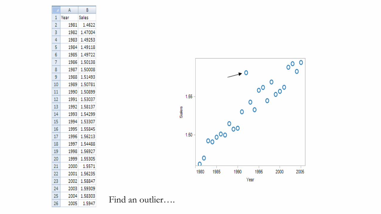
Find an outlier….

Visual perception

11

70% 30%

Mechanics of sight

StimulusSensory organ

Perceptual organ

12

Sensation(physical process)

Perception(cognitive process)

Eye

13

(pupila)

(čočka)(sítnice)

(fovea)

(žlutá skvrna)

(duhovka)

(rohovka)

rods (tyčinky), cones (čípky)

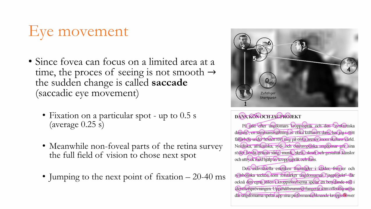
Eye movement

• Since fovea can focus on a limited area at a time, the proces of seeing is not smooth →the sudden change is called saccade(saccadic eye movement)

• Fixation on a particular spot - up to 0.5 s (average 0.25 s)

• Meanwhile non-foveal parts of the retina survey the full field of vision to chose next spot

• Jumping to the next point of fixation – 20-40 ms

15

Brain

16

StimulusSensory organ

Perceptual organ

Sensation(physical process)

Perception(cognitive process)

Iconic memory

(obrazová paměť)

Working memory

(krátkodobá paměť)

Long-term memory

(dlouhodobá paměť)

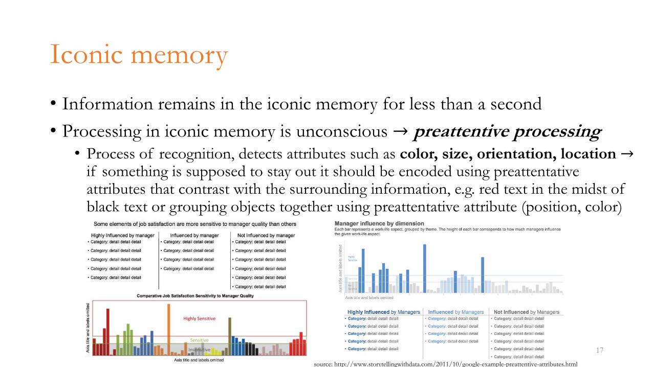
Iconic memory

• Information remains in the iconic memory for less than a second

• Processing in iconic memory is unconscious → preattentive processing• Process of recognition, detects attributes such as color, size, orientation, location→

if something is supposed to stay out it should be encoded using preattentativeattributes that contrast with the surrounding information, e.g. red text in the midst of black text or grouping objects together using preattentative attribute (position, color)

17

source: http://www.storytellingwithdata.com/2011/10/google-example-preattentive-attributes.html

Working memory

• Processing in working memory is conscious → attentive processing

• Data passed from iconic to working memory where they are combined and stored as visual chunks

• Characteristics• Temporary

• If not rehearsed, the chunks stays in iconic memory for only few seconds

• Limited storage capacity

• 3-4 chunks

• A reader can therefore hold only a few chunks of information in her head → a legend of a graph with 10 shapes or colors forces the reader to constantly refer back to the legend

18

Long-term memory

• When it is decided (consciously or unconsciously) that a chunk needs to be stored it is moved (by rehearsal) to long-term memory

• Long-term memory has the ability to recognize images and detect meaningful patterns

19

Attributes of preattentive processing

Category Form Color Spatial position Motion

Attribute

Length

Width

Orientation

Shape

Size

Enclosure

…

Hue

Intensity

2D/3D position Direction

20

• Visual attributes/encodings to be perceived by the preattentiveprocessing

3547876546879871846546546546544789132428735751486424484355454741111235431875843216546843213546846513135468435132516846513216594351351435435413217543513513543512131351321216874652135435171212233135121047687921212165121354646184357286456465498717316

21

3547876546879871846546546546544789132428735751486424484355454741111235431875843216546843213546846513135468435132516846513216594351351435435413217543513513543512131351321216874652135435171212233135121047687921212165121354646184357286456465498717316

Attentive processing – find the number of nines in the list as fast as you can

Preattentive processing – find the number of nines in the list as fast as you can

Preattentive attributes of form

22

Length Width Orientation

Shape Size Enclosure

Preattentive attributes of color (1)

23

Hue Intensity

Preattentive attributes of color (2)

• Color is made up from three attributes

24

Intensity applies to both saturation and lightness

Hue Saturation Lightness/Brightness

0% saturation 100% saturation 0% lightness 100% lightness

Preattentive attributes of spatial position

25

2D position

Preattentive attributes of motion (1)

26

Direction

Preattentive attributes of motion (2)

27

Encoding quantitative values

• Quantitative vs categorical difference

• Values represented as lines of different lengths are perceived as quantitatively different (longer lines greater values)

• Values represented as different colors are only categorically different (e.g., red is not “greater” than blue)

• However, e.g. intensity is perceived quantitatively

28

Type Attribute Quantitatively

perceived

Form Length Yes

Width Yes (limited)

Orientation No

Size Yes (limited)

Shape No

Enclosure No

Color Hue No

Intensity Yes (limited)

Position 2D position Yes

29

1 ?

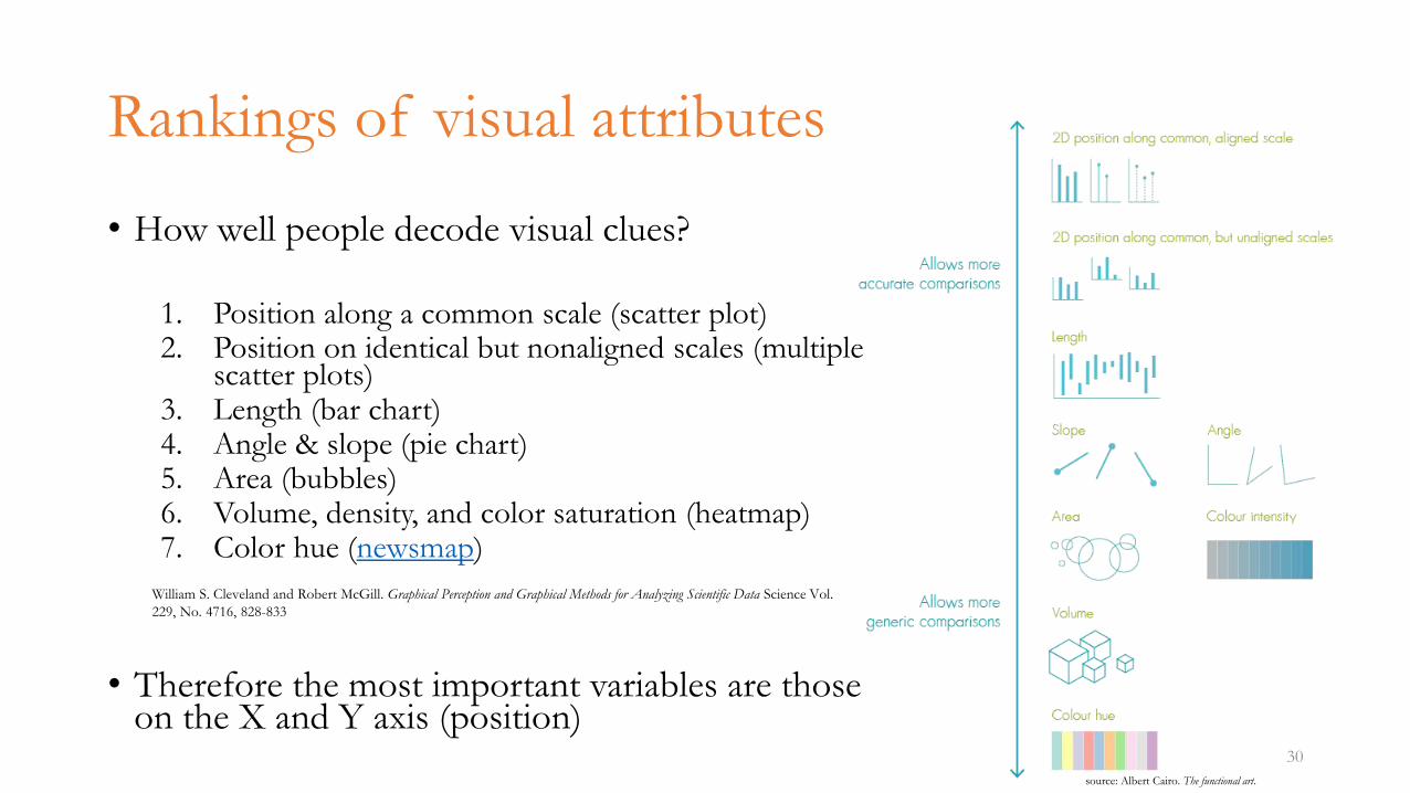
Rankings of visual attributes

• How well people decode visual clues?

1. Position along a common scale (scatter plot)2. Position on identical but nonaligned scales (multiple

scatter plots)3. Length (bar chart)4. Angle & slope (pie chart)5. Area (bubbles)6. Volume, density, and color saturation (heatmap)7. Color hue (newsmap)

• Therefore the most important variables are those on the X and Y axis (position)

30

William S. Cleveland and Robert McGill. Graphical Perception and Graphical Methods for Analyzing Scientific Data Science Vol.

229, No. 4716, 828-833

source: Albert Cairo. The functional art.

• Visual perception is deeply evolutionary ingrained

31

Evolutionary basis of visual perception

Effects of context

32

• Our visual senses are designed to perceive differences in values rather than absolute values

Limits to distinct perception (1)

• Too much visual attributes or values per attribute can harm

• “It is simple to spot a single hawk in a sky full of pigeons, but it would be more difficult if the sky contained more types of birds” (Ware, 2004)

• Using larger number of values forces readers to use the slower attentive processing which allows to store only up to four distinctive values at a time

33

Limits to distinct perception (2)

• Preattentive processing usually cannot handle more than one visual attribute of an object at a time

34

Focus on black objects Focus on white objects

Focus on white squares

Limits to distinct perception (3)

• There are nine hues that are easy to recognize

Gray

Blue

Orange

Green

Pink

Brown

Purple

Yellow

Red

Soothing colors, suitable for tables and graphs.

Vibrant colors, suitable for highliting.

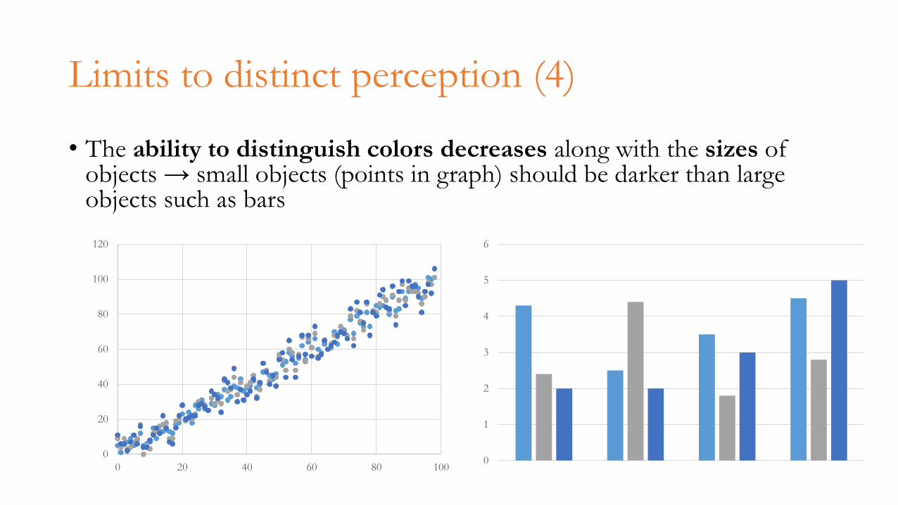
Limits to distinct perception (4)

• The ability to distinguish colors decreases along with the sizes of objects → small objects (points in graph) should be darker than large objects such as bars

0

20

40

60

80

100

120

0 20 40 60 80 1000

1

2

3

4

5

6

Gestalt principles of visual perception

• Gestalt (pattern, shape, form) school of psychology (introduced around 1900)• Focus on understanding how we perceive, understand and organize what we see

• Mind has self-organizing tendencies → Gestalt laws/principles of grouping

37

• Principle of proximity

• Principle of similarity

• Principle of enclosure

• Principle of closure

• Principle of continuity

• Principle of connection

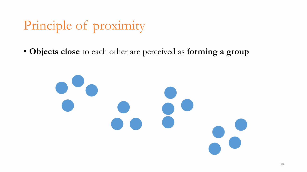
Principle of proximity

• Objects close to each other are perceived as forming a group

38

39

The principle of proximity can be used to

direct the reader to scan tables

predominantly row or column wise.

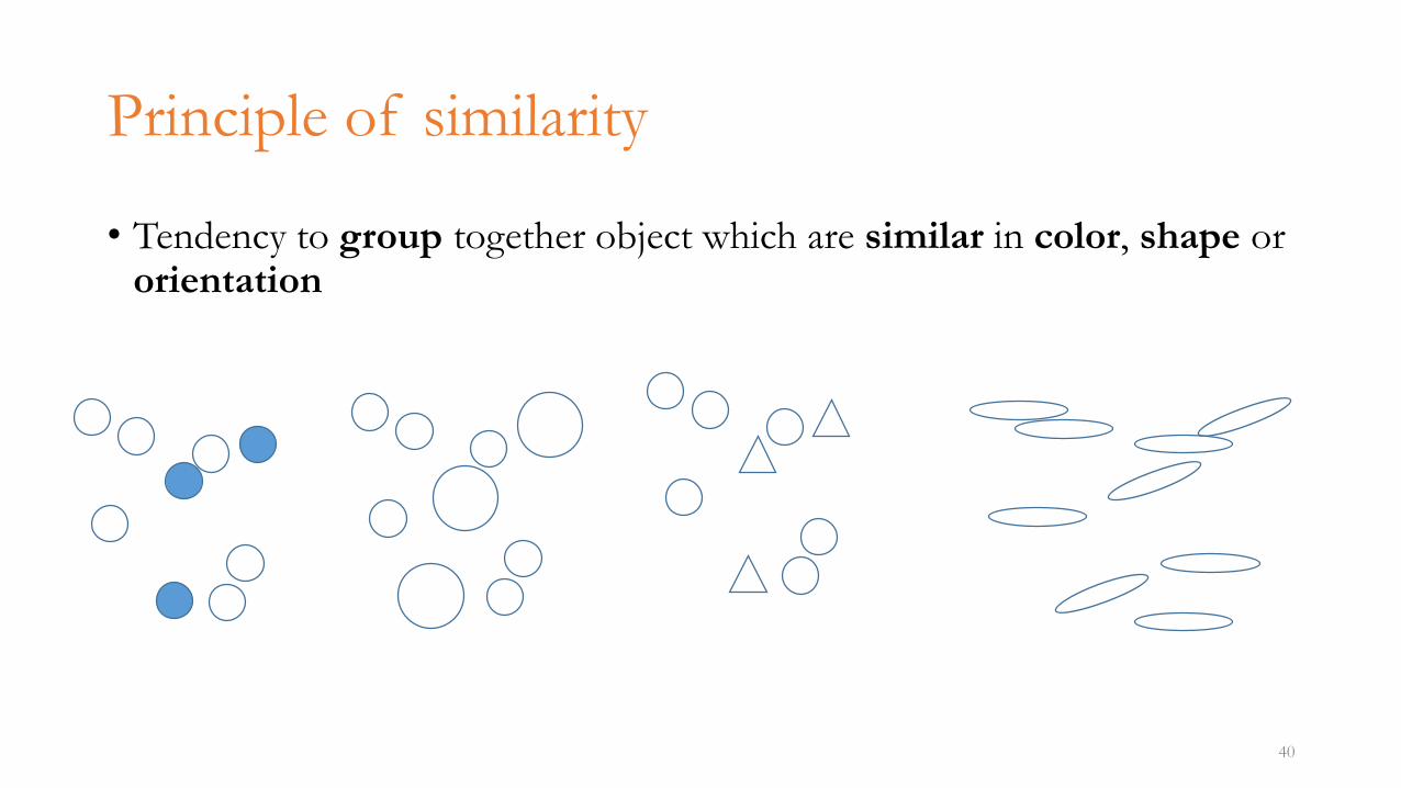
Principle of similarity

• Tendency to group together object which are similar in color, shape or orientation

40

xxxx

41

xxxx

xxxx

xxxx

xxxx

xxxx

xxxx

xxxx

xxxx

xxxx

xxxx

xxxx

xxxx

xxxx

xxxx

xxxx

xxxx

xxxx

xxxx

xxxx

xxxx

xxxx

xxxx

xxxx

xxxx

xxxx

xxxx

xxxx

xxxx

xxxx

xxxx

xxxx

xxxx

xxxx

xxxx

xxxx

xxxx

xxxx

xxxx

xxxx

xxxx

xxxx

xxxx

xxxx

xxxx

xxxx

xxxx

xxxx

Principle of enclosure

• We perceive objects belonging together when they are somehow enclosed

42

Principle of closure

• If there is an ambiguous stimuli we will try to eliminate the ambiguity

• We prefer to see objects as closed, complete and regular

43

Principle of continuity

• We perceive objects as belonging together, forming a whole, if they are aligned or connected to one another

44

0 1 2 3 4 5 6

Category 1

Category 2

Category 3

Category 4

Series 3 Series 2 Series 1

45

Due to the principle of continuity there is no need for the “0” line

Principle of connection

• Connected objects are perceived as part of a group

• Connection exercises greater power than proximity or similarity but less than enclosure

46

47

Data types

Quantitative data

• Deal with numbers

• Can be measured

• Stored in numeric variables

• Length, height, area, volume, weight, speed, time, temperature, humidity

Categorical/qualitative data

• Deals with descriptions

• Can be observed but not measured

• Stored in categorical variables

• Gender, color, texture, taste, appearance

48

Quantitative

• 120 x 100 cm

• Weights 0,5kg

• 2 people

• 1 animal

Qualitative

• Aquarelle

• Darker colors

• Contains text

• Masterful brush strokes

49

Quantitative relationships

• Quantitative stories are about relationships which, in turn, determine the type of visualization to relay the story (table, graph, diagram, …)

50

Quantitative information Relationship

Units of product sold per geographical location Sales related to geography

Revenue by quarter Revenue related to time

Expenses by department and month Expenses related to organization structure and time

A company’s market share compared to that of its

competitors

Market share related to companies

The number of employees who received each of the

five possible performance ratings during the last

annual performance review

Employee counts related to performance ratings

Quantitative data vs

categorical data

Relationships between categories

Categorical items used to label corresponding measures relate to one another in the following ways

51

Nominal (jmenné)

• Values in a single category are discrete and have no intrinsic order

• Sales in regions (East, West, North, South)

Ordinal (pořadové)

• The categorical items have order

• Size (small, medium, large)

Interval (měřitelné, intervalové)

• Categorical items consist of a sequential series of numerical ranges

• Order size ($0-$1,000;$1,000-$2,000;>$2,000)

Hierarchical (hierarchické)

• Involves multiple categories in the parent-child relation (tree structure)

• Organizational structure (division → department → group [→ expenses])

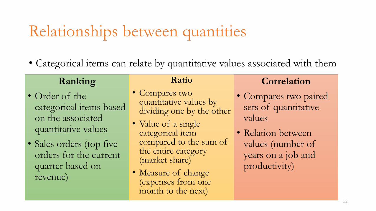
Relationships between quantities

• Categorical items can relate by quantitative values associated with them

52

Ranking

• Order of the categorical items based on the associated quantitative values

• Sales orders (top five orders for the current quarter based on revenue)

Ratio

• Compares two quantitative values by dividing one by the other

• Value of a single categorical item compared to the sum of the entire category (market share)

• Measure of change (expenses from one month to the next)

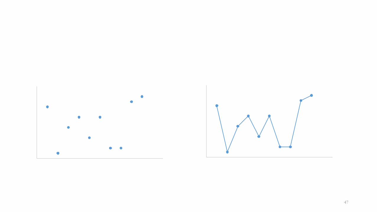
Correlation

• Compares two paired sets of quantitative values

• Relation between values (number of years on a job and productivity)

Numbers that summarize

• Ways to summarize/aggregate data → descriptive statistics

• Reduces large sets of data allowing to comprehend the story

• Measures of average (central tendency, center)

• Measures of variation

• Measures of correlation

• Measures of ratio

53

Measures of average (1)

(Arithmetic) Mean

• Sum of all the values divided by the number of values

• Measure of center taking into account all values → prone to be influenced by extreme values

• E.g., in case of salaries it can be used to show comparative impact of departments of a company on expenses

Median

• Value from the middle of the (sorted) set

• Expresses the typical values

• E.g., in case of salaries it can be used to show typical salary (per department)

54

Measures of average (2)

Mode

• The specific value that appears most often in the set

• If there are more values like this, the set is multimodal

• If there is no such value, the set does not have a mode

Midrange

• The value midway between highest and lowest value

• Quick estimate of center

• Very sensitive to extremes (if the distribution is not uniform)

55

Measures of variation (1)

• Presents the degree into which values vary

56

Spread

• Difference between the lowest and the highest value

• Relies on too little information

• Affected by extreme values

Standard deviation

• Measures variation in a set relativeto mean

• The higher the number of values the less it is prone to bias due to the extreme values

Measures of variation (2)

• High variation in time it takes to manufacture products, answer phone calls, or resolve technical calls• Does it indicate problems in training, process design, or systems?

• Variation in departmental expenses.• Do some departments manage to keep their expenses much lower than others?

Why?

• Variation in food quality of a restaurant reported by customers.• Does the variation relate to the cook?

57

Measures of correlation

• The simples relation we measure is linear correlation being commonly expressed in terms of the (Pearson) correlation coefficient

• Ranges between -1 (strongest negative correlation) and 1 (strongest positive correlation)

58corr(x,y) = 0,816

Measure of ratio

• Measures relation between a single pair of values (unlike correlation)

• Can be expressed in the following ways

59

• Special use case is setting one of the values constant → baseline to which other value are compared (set to 1 or 100%)

Sentence

Two out of every five customers who

access our website place an order

Fraction

2/5

Rate

0.4 (i.e., the result of division 2/5)

Percentage

40% (i.e., the 0.4 rate multiplied by 100)

0

50

100

150

200

250

Company A Company B Company C Company D

Our company

General data sources

• World Bank

• EU Open Data Portal

• Eurostat

• data.gov.uk

• U.S. Government’s open data

• OECD

• Knoema

• OpenData.cz

• Data Portals

• Tableau

• ManyEyes

• ….

60

“Big data” repositories

• Click (2.5 TB)

• Tiny images (227 GB)

• Wikipedia edits (2GB)

• 1000 genomes project (260 TB)

• ….

61

Machine learning related repositories

• Kaggle datasets

• Kdnuggets datasets

• mldata

• http://archive.ics.uci.edu/ml/

• ….

62

Sources

• Stephen Few (2012) Show Me the Numbers – Designing Graphs and Tables to Enlighten

63