data structures recursion phil tayco slide version 1.0 mar. 8, 2015

Data StructuresRecursion

Phil Tayco

Slide version 1.0

Mar. 8, 2015

Recursion

Algorithm categories

• We are used to seeing code written following the 3 categories of programming:– Sequence: Statements that are linearly executed one

after the other– Selection: If…else statements that have branching paths

of execution– Repetition: Loop statements that repeat based on a

condition• The language syntax is easy to follow once the

fundamentals of programming are understood

Recursion

A different representation

• Some algorithms can be stated as functions similar to mathematical induction for solving series:– Base case: the part of the solution that is represents the

first element of the series– Inductive case: the “rest” of the solution that states the

remainder of the series in terms of itself• In computer science, this approach is used for

algorithms that fit into this form of problem solving

• Instead of specifying the sequential steps of the solution, the function is inductively stated

Recursion

Factorials

• Start with a math example• A factorial is an integer multiplied by the each number in

the series from that number descending to one• Represented with an exclamation point, examples include:

– 5! = 5 * 4 * 3 * 2 * 1– 4! = 4 * 3 * 2 * 1– 3! = 3 * 2 * 1– 2! = 2 * 1– 1! = 1

• No negative number factorials can be performed• The factorial of 0 is 1

Recursion

Patterns

• Notice those answers can be restated:– 1! = 1– 2! = 2 * 1 = 2 * 1!– 3! = 3 * 2 * 1 = 3 * 2!– 4! = 4 * 3 * 2 * 1 = 4 * 3!

• Or restated in general terms:– n! = n * (n – 1)!

• The factorials of 0 and 1 are also 1. They don’t fit the general case so we consider these to be special (or base) cases

• Put the two together and you can state that the factorial for any given number n (assuming negative numbers are already excluded):

– If n = 0 or n = 1, the answer is 1– If n > 1, the answer is n * (n – 1)!

• We refer to the first part as the base case and the second as the inductive case (also called the general case or the recursive case)

• This can be stated the same way in program code

Recursion

long factorial (int n)

{

if (n == 0 || n == 1)

return 1;

return n * factorial(n – 1);

}

Recursion

Code analysis

• The code is simple in terms of number of lines and following the mathematical model, but can be complex in terms of trying to understand the program flow of control

• The code contains a line that calls a function which happens to be itself. This is the part of the code that is using the “recursion” technique

• The recursion is essentially another way of performing a loop. Each time the recursion occurs, another version of the function is executed just like any other function call that occurs

• Note that each time the recursive function call is made, the value passed in is different than the value that it was given. In this case, we pass into the next function call a value of (n-1)

• Eventually, the recursive function calls must stop, this is when the base case is reached. Notice with each recursive, the value of n passed in goes down by 1. This will reach 1 at some point

• When the base case is reached, the simple value of 1 in this case is returned. All the recursive function calls that were made are now “unwound”

Recursion

Graphical view of “x = factorial(3);”

main()

x = factorial(3);

factorial(n = 3)

return 3 * factorial (3 – 1);

factorial(n = 2)


Recursion

Recursion analysis 1

• The main function begins with a standard function call to factorial passing a value of 3

• In the first instance of factorial(3), the base case check is false (n does not equal 0 nor 1)

• Therefore, in factorial(3), the line “return n * factorial(n-1);” is executed

• This temporarily halts execution in factorial(3) as it must wait for the return of factorial(n-1)

• This takes us to the next function instance of factorial(2)• Note that factorial(3) and factorial(2) are separate execution

instances just like any other function call. These function calls just happen to be using the same code

• The same sequence occurs in factorial(2) where another recursive function call will take place to factorial(1)…

Recursion


main()

x = factorial(3);

factorial(n = 3)


factorial(n = 2)


factorial(n = 1)

return 1;

Recursion


• In the function instance of factorial(1), the base case is now reached

• No further recursive function calls occur, and a value of 1 is returned

• Like any other function that completes, the return value goes back to the original function call for use

• In this case the original function call is the previous instance of itself and the “unwinding” begins

Recursion


main()

x = factorial(3);

factorial(n = 3)


factorial(n = 2)

return 2 * 1;

1

Recursion


• factorial(2) was the instance that made the function call to factorial(1)

• factorial(1) reached the base case and simply returns a value of 1

• That value comes back to factorial(2) at the point where the function call was made

• That point is in the line “return n * factorial(n-1);”• In this instance, then, the line of code in factorial(2) is now

“return 2 * 1;” because the recursive function call is replaced with that function’s return value

• This results in a “return 2;” which now continues the unwinding by returning that value to factorial(2)’s original function caller which was factorial(3)…

Recursion


main()

x = factorial(3);

factorial(n = 3)

return 3 * 2;

2

Recursion


• factorial(3) now receives the return value of 2 exactly like factorial(2) received the return value of 1 from factorial(1)

• That value of 2 is applied to the line it was called from which will result in “return 3 * 2;” in the factorial(3) function

• The unwinding now completes with factorial(3) returning a value of 6 back to its original function caller. In this example, that function is main

• main called factorial(3) and is assigning that function’s return value into x and thus completing the recursive line of execution

Recursion


main()

x = 6;

6

Recursion

Function call stack

• Recall in the stacks and queues discussion that one of the examples of using a stack is function call management

• When a function is called, in instance of that function is pushed onto the stack and executes as coded. When the function completes, the instance is popped from the stack any value returned is passed back into the next instance on top at the point where it made its function call

• The same process is happening with recursion. The key difference is that the function instances created are using the same function code

• The recursive functions are using the same code, but the logical design of the base and inductive cases set it up so that the recursive loop will eventually end when the base case is reached

Recursion

Practice, practice, practice

• Understanding recursion is not trivial• Just like other programming concepts,

understanding the theory and the code starts with practicing different algorithms and walking through the code, line by line

• In this case, following the function call stack is necessary as well. It is very easy to get lost in the recursion without the visualization

• Another famous example and mathematical sequence: Fibonacci numbers

Recursion

Theory and efficiency

• Can this factorial example be written without recursion? Of course! In previous classes, you probably did it with a for or while loop

• In theory, any recursive loop can be written as a standard loop

Recursion

Fibonacci numbers

• The Fibonacci number sequence is:– 0, 1, 1, 2, 3, 5, 8, 13, 21, 34, …

• What is the pattern in this sequence? Starting at Fibonacci number 3, the number equals the sum of the previous 2 numbers:

– Fib at location 3 = 1 which equals 0 + 1 which equals Fib at 1 + Fib at 2– Fib at location 4 = 2 which equals 1 + 1 which equals Fib at 2 + Fib at 3– Fib at location 5 = 3 which equals 1 + 2 which equals Fib at 3 + Fib at 4– Fib at location 6 = 5 which equals 2 + 3 which equals Fib at 4 + Fib at 5

• Like we did with the factorial, we can restate this in general terms:– Fib at location n = Fib at location (n – 1) + Fib at location (n – 2)

• The Fibonacci numbers at locations 1 and 2 don’t fit the general case which imply that these are the base cases

• Put the two together and you can state that finding the Fibonacci number at location n is:

– If n = 1, the answer is 0– If n = 2, the answer is 1– If n > 2, the answer is Fib(n-2) + Fib(n-1)

• Given this and our current understanding of recursive programming, the code is a near direct translation of the formula

Recursion

int fib(int n)

{

if (n <= 1)

return 0;

if (n == 2)

return 1;

return fib(n-2) + fib(n-1);

}

Recursion

Code analysis

• The base cases and inductive case follows a similar pattern as the factorial

• Notice here that the line of code with the recursion is making 2 recursive functions calls on the same line

• This means if the recursive line is reached, 2 recursive calls are handled before that value is returned

• Practice understanding this by drawing the function call stack and following the execution with “x = fib(4);”

• If you can do this on your own and feel comfortable with it, you have a nice start to understanding recursion

Recursion

Main calls fib(4). In fib(4), base cases are not true. Thus, we call return fib(2) + fib(3);

main()

x = fib(4);

fib(n = 4)

return fib(2) + fib(3);

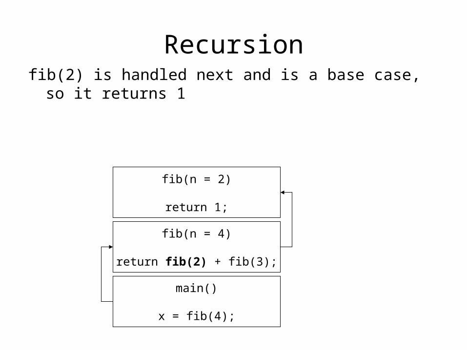
Recursionfib(2) is handled next and is a base case, so it

returns 1

main()

x = fib(4);

fib(n = 4)


fib(n = 2)

return 1;

Recursion1 is returned back to fib(4) where fib(2) was called.

Now the fib(3) part of the code must be executed

main()

x = fib(4);

fib(n = 4)

return 1+ fib(3);

1

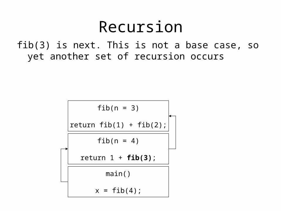
Recursionfib(3) is next. This is not a base case, so yet another

set of recursion occurs

main()

x = fib(4);

fib(n = 4)

return 1 + fib(3);

fib(n = 3)


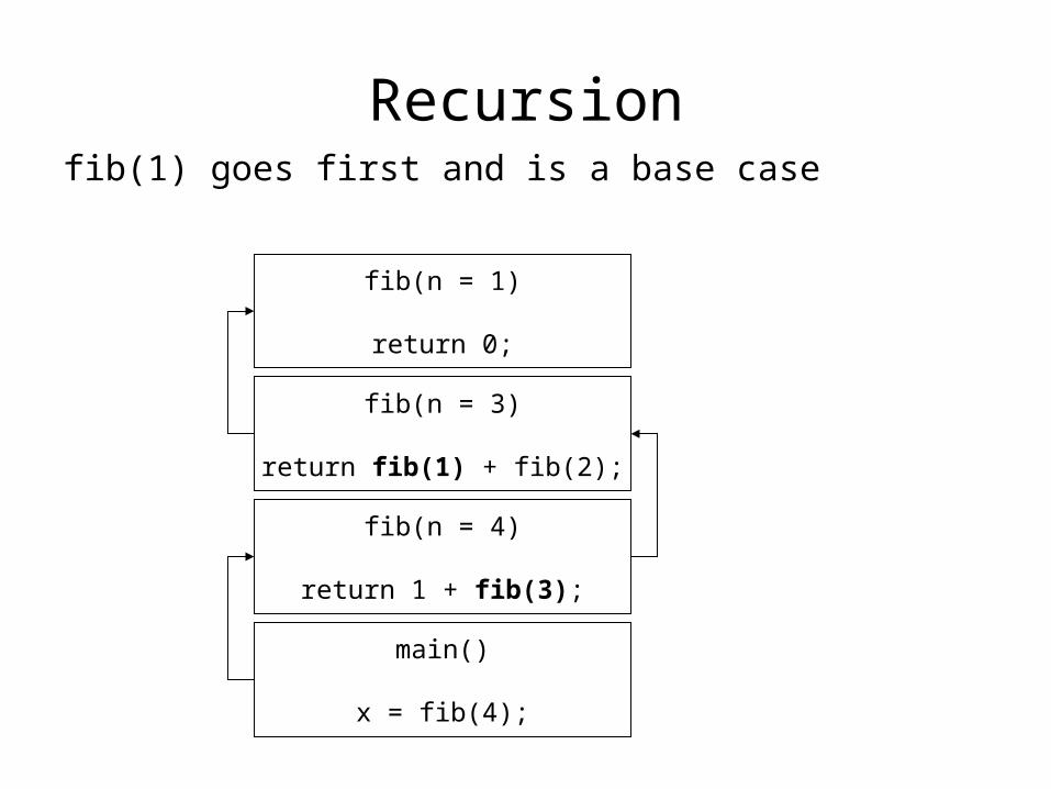
Recursionfib(1) goes first and is a base case

main()

x = fib(4);

fib(n = 4)

return 1 + fib(3);

fib(n = 3)


fib(n = 1)

return 0;

Recursion0 is returned from fib(1). Back in fib(3), we call

fib(2) which we already know will return 1

main()

x = fib(4);

fib(n = 4)

return 1 + fib(3);

fib(n = 3)

return 0 + fib(2);

0

Recursionfib(3) is now complete and will return 0+1 to fib(4)

main()

x = fib(4);

fib(n = 4)

return 1 + fib(3);

fib(n = 3)

return 0 + 1;

RecursionWith fib(3) complete for fib(4), fib(4)’s recursion is

now complete and will return 2 to main and complete all the recursion

main()

x = fib(4);

fib(n = 4)

return 1+ 1;

1

RecursionAll done!

main()

x = 2;

2

Recursion

Recursive Fibonacci analysis

• Note again that the process of calling a function, pushing the new function onto the stack for processing and returning to the point of the function call is consistent whether it’s a call to another function or a recursive call

• Understanding the recursion call process requires drawing out the different function instances and tracing the flow of control

• Simple mathematical series that can be stated inductively are classic cases for recursion, but are not the only ones

• A famous recursive function example is the Towers of Hanoi

Recursion

The Legend of the Towers of Hanoi

• An Asian monk is tasked with transferring 64 disks from one pillar to another

• Each disk is different in size with a smaller disk always on top of a larger disk (making the 64th disk on the bottom the largest of them all)

• The are three pillars total (call them A, B and C) and all 64 disks are on pillar A

• The goal is to get them all to C following 2 rules:– Only one disk can move at a time– A larger disk cannot rest on top of a smaller disk

• When all 64 disks are transferred, the world ends

Recursion

Algorithm

• Assuming it takes one second to move a disk and he started right now, how long before the world ends?

• More importantly for us, what is the algorithm to do this?

• Obviously, in the current context, recursion is involved, but developing this algorithm is not as intuitive as the previous examples

• As with other situations, work out solutions with smaller values to derive the base and inductive cases

• Let’s start with 1 disk instead of 64

Recursion

With one disk, the move is obvious. Move disk from A to C. Another way to say it is we are moving the disk from start to destination

A B C

Recursion

Another way to say it is we are moving the disk from start to destination.

A B C

Recursion

Establish our base

• The move from start to destination is occurring with 1 disk

• Stated another way, if we are looking at one disk, move it to where you want it to go

• This sounds like a base case, but may seem peculiar given that the overall rules for the problem is that you can only move one disk at a time anyway

• Let’s move to the 2 disk situation

Recursion

Here, if we move the first disk on A to C, the next disk on A won’t be able to go to C without the smaller one out of the way

A B C

Recursion

Step 1: Move disk from A to B. B acts as a “temporary” pillar, while A and C are “start” and “destination” pillars respectively

A B C

Recursion

Step 2: Now we can move the disk from A (start) to C (destination)

A B C

Recursion

Step 3: Last move is simple. From disk from B (temp) to C (destination)

A B C

Recursion

2 disk case

• The 2 disk situation shows a key 3 step process – Move 1 disk from start to temp– Move 1 disk from start to destination– Move 1 disk from temp to destination

• The idea that one pillar serves as a “temporary” one while the other two are start and destination is critical to understanding the solution

• The ultimate goal is A to C for all disks, but along the way, what is “start”, “temporary” and “destination” will differ depending on your situation

• Now let’s bump it up to 3 disks keeping in mind the reasoning behind the simple steps for 2 disks

Recursion

Start. Where do we go from here?

A B C

RecursionIf we follow the same moves (A to B, A to C, B to C),

we would have 2 disks at C, but the one big disk still at A. Thus, we should not end up with these 2 disks on C

A B C

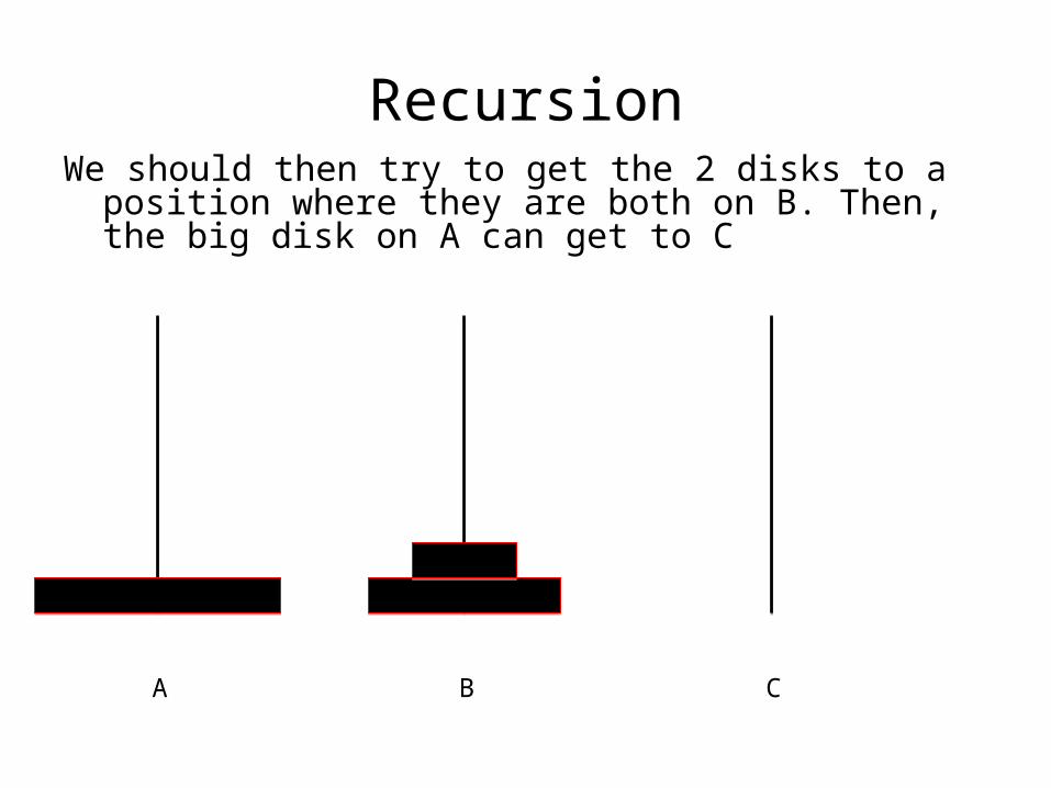
RecursionWe should then try to get the 2 disks to a position

where they are both on B. Then, the big disk on A can get to C

A B C

RecursionHow do we get to that point? Note that for these 2

disks, the steps in the previous example apply, but B would be our “destination” and C would be our “temp”

A (start) B (dest) C (temp)

RecursionGiven these labels, the 3 moves are the same as

before. Step 1: Move A to C (start to temp)


RecursionStep 2: Move A to B (start to dest)


RecursionStep 3: Move C (temp) to B (dest). Note now that

this temporary 2 disk goal of getting them to destination B is complete


RecursionIn the overall picture for 3 disks, our destination is C

and at this point, we have successfully moved 2 disks off A to the temporary pillar B

A (start) B (temp) C (dest)

Recursion

3 disk case so far

• Recall the steps when there are only 2 disks– Move 1 disk from start to temp– Move 1 disk from start to destination– Move 1 disk from temp to destination

• We’ve actually done the first step of this with 3 disks, ending up with moving 2 disks to temp

• This opens the door to generalizing the 3 step process doing so in inductive terms:– Move (n-1) disks from start to temp– Move 1 disk from start to destination– Move 1 disk from temp to destination

• Now let’s see if the 2nd step still applies

RecursionStep 4: Move A to C (temp to dest)


Recursion

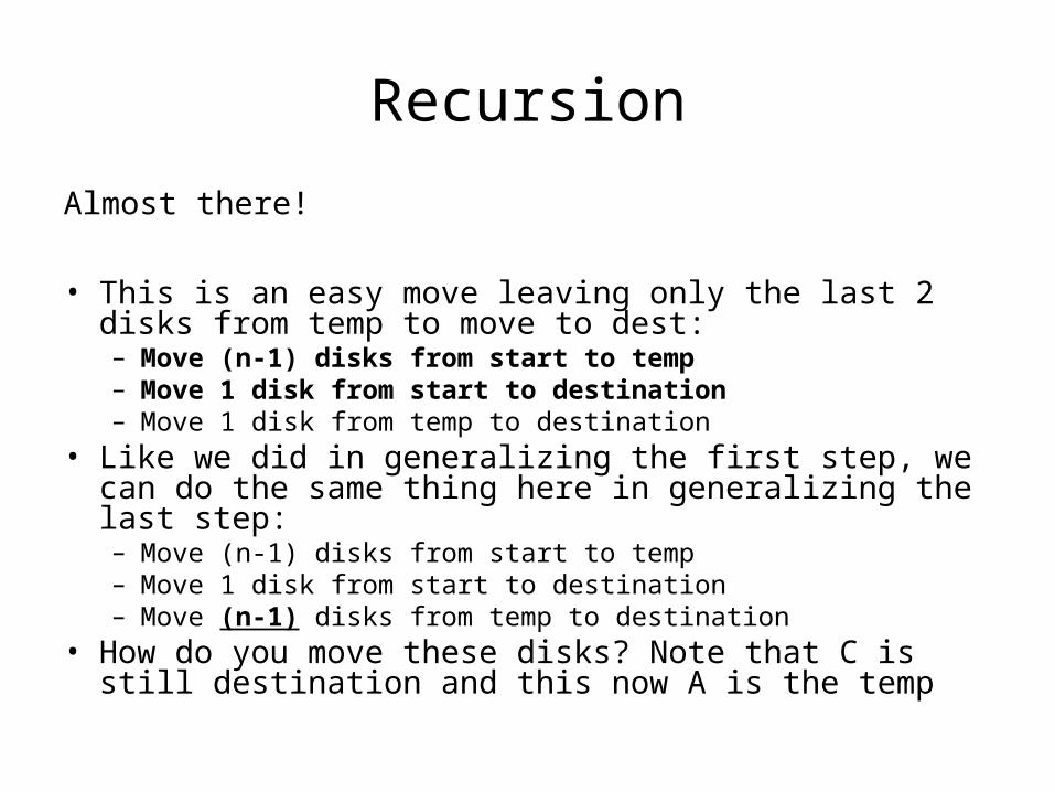
Almost there!

• This is an easy move leaving only the last 2 disks from temp to move to dest:– Move (n-1) disks from start to temp– Move 1 disk from start to destination– Move 1 disk from temp to destination

• Like we did in generalizing the first step, we can do the same thing here in generalizing the last step:– Move (n-1) disks from start to temp– Move 1 disk from start to destination– Move (n-1) disks from temp to destination

• How do you move these disks? Note that C is still destination and this now A is the temp

RecursionStep 5: Move B to A (start to temp)

A (temp) B (start) C (dest)

RecursionStep 6: Move B to C (start to dest)


RecursionStep 7: Move A to C (temp to dest)


Recursion

Done! So what’s the formula?

• The general case is complete:– Move (n-1) disks from start to temp– Move 1 disk from start to destination– Move (n-1) disks from temp to destination

• The base case is simply to move the disk using the same terminology:– If n=1, move the disk from start to destination

• Now the program this in recursive code, we need key information of the number of disks and where the “start”, “temp” and “destination” pillars are

• We can start with a function signature

Recursionvoid hanoi(int n, char start, char temp, char dest){}

main(){

hanoi (3, ‘A’, ‘B’, ‘C’);}

The main function calls hanoi saying let’s move 3 disks from A to C with B as our temp

The hanoi function signature matches itNow let’s do the base case

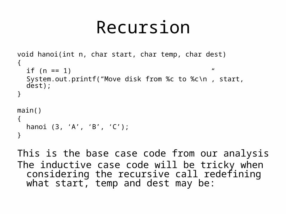
Recursionvoid hanoi(int n, char start, char temp, char dest){

if (n == 1)System.out.printf(“Move disk from %c to %c\

n”, start, dest);}

main(){

hanoi (3, ‘A’, ‘B’, ‘C’);}

This is the base case code from our analysisThe inductive case code will be tricky when

considering the recursive call redefining what start, temp and dest may be:

Recursionvoid hanoi(int n, char start, char temp, char dest){

if (n == 1)System.out.printf(“Move disk from %c to %c\

n”, start, dest);else{

hanoi(n-1, start, dest, temp);System.out.printf(“Move disk from %c to %c\

n”, start, dest);hanoi(n-1, temp, start, dest);

}}

Recursion

That’s it?!

• That’s it! The only way to truly internalize this is to walk through the code

• Like with factorial and Fibonacci, tracing through the function call stack is important

• Let’s do that again here with attempting to move 2 disks from A to C with B as our temp

Recursion

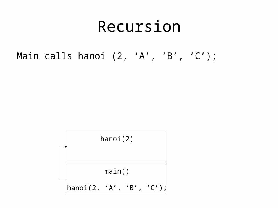
Main calls hanoi (2, ‘A’, ‘B’, ‘C’);

main()

hanoi(2, ‘A’, ‘B’, ‘C’);

hanoi(2)

Recursion

hanoi(2) is not a base case, so we go to the inductive case starting with hanoi(2-1, ‘A’, ‘C’, ‘B’); Do you see why the function call values are in that order?

main()

hanoi(2, ‘A’, ‘B’, ‘C’);

hanoi(2)

hanoi(1, ‘A’, ‘C’, ‘B’);print(“A to C”);

hanoi(1, ‘B’, ‘A’, ‘C’);

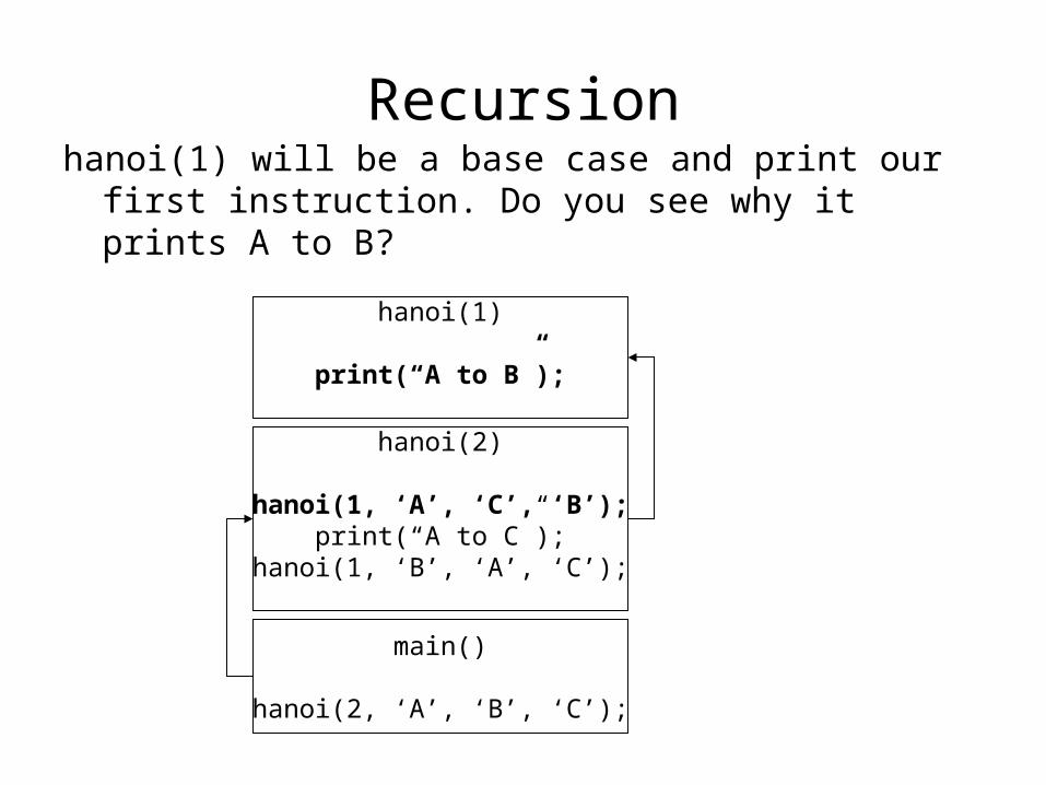
Recursionhanoi(1) will be a base case and print our first

instruction. Do you see why it prints A to B?

main()

hanoi(2, ‘A’, ‘B’, ‘C’);

hanoi(2)


hanoi(1, ‘B’, ‘A’, ‘C’);

hanoi(1)

print(“A to B”);

Recursionhanoi(1) is done and we return to hanoi(2). Next

code in hanoi 2 is another print

main()

hanoi(2, ‘A’, ‘B’, ‘C’);

hanoi(2)


hanoi(1, ‘B’, ‘A’, ‘C’);

Output so far:

Move A to B

Recursionhanoi(2) continues with the last line of its inductive

step and gets ready to make another recursive call. Note again the order of the function call values

main()

hanoi(2, ‘A’, ‘B’, ‘C’);

hanoi(2)


hanoi(1, ‘B’, ‘A’, ‘C’);

Output so far:

Move A to BMove A to C

Recursionhanoi(1) is another base case with different start

and dest values

main()

hanoi(2, ‘A’, ‘B’, ‘C’);

hanoi(2)


hanoi(1, ‘B’, ‘A’, ‘C’);

Output so far:

Move A to BMove A to C

hanoi(1)

print(“B to C”);

Recursionhanoi(1) and then hanoi(2) will be done and we

return to main with the correct output on the screen!

main()

hanoi(2, ‘A’, ‘B’, ‘C’);

Output so far:

Move A to BMove A to CMove B to C

Recursion

Code is beautiful

• This is a key (and historic) example of the Towers of Hanoi solution

• Tracing through with only 2 disks may be interesting, but to truly appreciate it in action, trace through the code with 3 or 4 disks. This is an excellent way to practice recursion

Recursion

Analysis

• How many steps will we see with 3 disks? How many with 4? Can you generalize it to a formula?– 1 disk = 1 move– 2 disks = 3 moves– 3 disks = 7 moves– 4 = 15 moves– N = 2n – 1

• Subsequently, 64 disks equals 1.84 x 1019

• At one move per second, this works out to about 585 billion years, with no breaks. We have time before the end of the world…

RecursionPerformance

• Analyzing the Big-O for comparisons with recursive solutions is noteworthy, but often not seen as an improvement to a solution

• Moreover, the function call stack is heavily utilized making recursion higher in memory usage

• Functions like factorial and Fibonacci can probably perform faster and use memory better using standard loops

• Hanoi and some other solutions we’ll see, though, could be a challenge to do iteratively versus with recursion

• Thus, recursive solutions are beneficial in developing a functional algorithm, but not necessarily for performance and memory usage

RecursionSummary

• Practice, practice, practice. Understanding recursive code by tracing is the first step

• There are many problems that have potential recursive solutions. Once you are able to read and trace recursive code, the next big challenge is learning how to develop a recursive algorithm

• The key is learning how to identify base and inductive cases. They are not easy to do, but very gratifying when developed

• Examples of other solutions always help too. We will see more as we revisit the advanced sorting algorithms next…

data structures recursion phil tayco slide version 1.0 mar. 8, 2015

Documents