data structures and amortized complexity in a functional - citeseer
TRANSCRIPT

i
Data Structures
and
Amortized Complexity
in a
Functional Setting
Berry Schoenmakers
Doctoral Dissertation fromEindhoven University of Technology
September 1992

ii
Acknowledgements
First of all, I would like to thank Anne Kaldewaij for his continuous supportand guidance over the past four years. We both enjoyed working on the subjectof amortization and learned a lot of interesting new things. Also, I very muchappreciate his advice to write and explain things in a relaxed pace (and whichhe demonstrated to me every so often).
Lex Bijlsma, Victor Dielissen, and Wim Nuij are gratefully acknowledgedfor discussing and reading together with Anne and me drafts of this thesis andrelated work. In particular, Wim Nuij is acknowledged for providing me withthe basis for Lemma 11.6.
Ronald Heutinck is acknowledged for his initial study of Fibonacci heapswhich led to the notion of “diagonal bags” [15]. The late Peter van den Hurkis acknowledged for his study (see [18, Chapter 3]) of the path/insert problem[19], which triggered the research reported in Section 3.2.
I thank Wim Kloosterhuis for his assistance with some of the mathematicsin the analyses of bottom-up melding and splaying.
Finally, Daniel D. Sleator is acknowledged for his referee’s report of [21] inwhich he presented an improved analysis of top-down melding.

iii
Contents
Introduction 1
I Theoretical Aspects 7
1 Algebras 81.1 Basic data types and operations . . . . . . . . . . . . . . . . . . . 9
1.1.1 Tuples . . . . . . . . . . . . . . . . . . . . . . . . . . . . . 91.1.2 Relations and functions . . . . . . . . . . . . . . . . . . . 91.1.3 Simple data types . . . . . . . . . . . . . . . . . . . . . . 101.1.4 Structured data types . . . . . . . . . . . . . . . . . . . . 11
1.2 Algebras . . . . . . . . . . . . . . . . . . . . . . . . . . . . . . . . 121.3 Monoalgebras . . . . . . . . . . . . . . . . . . . . . . . . . . . . . 17
2 Algebra refinement 202.1 Functional programs and specifications . . . . . . . . . . . . . . . 202.2 Algorithmic refinement of functions . . . . . . . . . . . . . . . . . 222.3 Data refinement of functions . . . . . . . . . . . . . . . . . . . . . 232.4 Refinement of monoalgebras . . . . . . . . . . . . . . . . . . . . . 262.5 Surjectivity and injectivity of monoalgebras . . . . . . . . . . . . 302.6 A closer look at surjectivity and injectivity . . . . . . . . . . . . 36
3 Amortized complexity 393.1 Amortized analysis of imperative programs . . . . . . . . . . . . 403.2 Abstract views of amortization . . . . . . . . . . . . . . . . . . . 44
4 Implementation aspects 494.1 Functional program notation . . . . . . . . . . . . . . . . . . . . 504.2 Eager evaluation . . . . . . . . . . . . . . . . . . . . . . . . . . . 514.3 Pointer implementation of stacks . . . . . . . . . . . . . . . . . . 524.4 Destructivity . . . . . . . . . . . . . . . . . . . . . . . . . . . . . 544.5 Queues and concatenable deques . . . . . . . . . . . . . . . . . . 55

iv Contents
4.6 Linear usage of destructive monoalgebras . . . . . . . . . . . . . 584.7 Benevolent side-effects . . . . . . . . . . . . . . . . . . . . . . . . 61
5 Analysis of functional programs and algebras 635.1 Cost measures . . . . . . . . . . . . . . . . . . . . . . . . . . . . . 635.2 Worst-case analysis . . . . . . . . . . . . . . . . . . . . . . . . . . 675.3 Amortized cost of functions . . . . . . . . . . . . . . . . . . . . . 695.4 Amortized analysis . . . . . . . . . . . . . . . . . . . . . . . . . . 715.5 Amortization and linearity . . . . . . . . . . . . . . . . . . . . . . 745.6 Purely-functional deques . . . . . . . . . . . . . . . . . . . . . . . 75
5.6.1 Specification and implementation . . . . . . . . . . . . . . 755.6.2 Some applications and their analyses . . . . . . . . . . . . 785.6.3 Comparison with doubly-linked list representation . . . . 82
6 More on lists and trees 846.1 Lists . . . . . . . . . . . . . . . . . . . . . . . . . . . . . . . . . . 85
6.1.1 Stacks with deletion . . . . . . . . . . . . . . . . . . . . . 866.1.2 Partitions . . . . . . . . . . . . . . . . . . . . . . . . . . . 87
6.2 Binary trees . . . . . . . . . . . . . . . . . . . . . . . . . . . . . . 876.2.1 Top-down views . . . . . . . . . . . . . . . . . . . . . . . 876.2.2 A skewed view . . . . . . . . . . . . . . . . . . . . . . . . 886.2.3 Root-path views . . . . . . . . . . . . . . . . . . . . . . . 90
6.3 Trees and forests . . . . . . . . . . . . . . . . . . . . . . . . . . . 926.3.1 Top-down views . . . . . . . . . . . . . . . . . . . . . . . 926.3.2 Root-path views . . . . . . . . . . . . . . . . . . . . . . . 93
6.4 Overview of tree types . . . . . . . . . . . . . . . . . . . . . . . . 94
II Case Studies 95
7 Tricky representations of sets and arrays 967.1 A tricky representation of sets . . . . . . . . . . . . . . . . . . . . 977.2 A tricky representation of arrays . . . . . . . . . . . . . . . . . . 997.3 Mehlhorn’s tricky representation of sets . . . . . . . . . . . . . . 1007.4 An unboundedly small potential . . . . . . . . . . . . . . . . . . 1017.5 Comparisons . . . . . . . . . . . . . . . . . . . . . . . . . . . . . 103
8 Maintaining the minimum of a list 1048.1 Stacks . . . . . . . . . . . . . . . . . . . . . . . . . . . . . . . . . 1048.2 Deques . . . . . . . . . . . . . . . . . . . . . . . . . . . . . . . . . 1068.3 Concatenable queues . . . . . . . . . . . . . . . . . . . . . . . . . 1068.4 Noninjective algebras . . . . . . . . . . . . . . . . . . . . . . . . . 107

Contents v
9 Skew heaps 1109.1 Priority queues . . . . . . . . . . . . . . . . . . . . . . . . . . . . 1109.2 Top-down skew heaps . . . . . . . . . . . . . . . . . . . . . . . . 112
9.2.1 Introduction of 1 . . . . . . . . . . . . . . . . . . . . . . . 1139.2.2 Implementation of 1 . . . . . . . . . . . . . . . . . . . . . 1149.2.3 Analysis of 1 . . . . . . . . . . . . . . . . . . . . . . . . . 1169.2.4 Refined analysis of 1 . . . . . . . . . . . . . . . . . . . . . 1209.2.5 Results for priority queue operations . . . . . . . . . . . . 1229.2.6 Comparison with Sleator and Tarjan’s results . . . . . . . 122
9.3 Intermezzo on sorting . . . . . . . . . . . . . . . . . . . . . . . . 1239.4 Bottom-up skew heaps . . . . . . . . . . . . . . . . . . . . . . . . 126
9.4.1 Implementation of MO . . . . . . . . . . . . . . . . . . . . . 1279.4.2 Bottom-up analysis of MO . . . . . . . . . . . . . . . . . . . 1299.4.3 First top-down analysis of MO . . . . . . . . . . . . . . . . . 1319.4.4 Second top-down analysis of MO . . . . . . . . . . . . . . . . 1399.4.5 Results for priority queue operations . . . . . . . . . . . . 142
9.5 Pointer implementations . . . . . . . . . . . . . . . . . . . . . . . 1429.6 Concluding remarks . . . . . . . . . . . . . . . . . . . . . . . . . 144
10 Fibonacci heaps 14610.1 Lazy binomial queues . . . . . . . . . . . . . . . . . . . . . . . . 14710.2 Intermezzo on the precondition of linking . . . . . . . . . . . . . 15110.3 Fibonacci heaps . . . . . . . . . . . . . . . . . . . . . . . . . . . . 15310.4 Concluding remarks . . . . . . . . . . . . . . . . . . . . . . . . . 158
11 Path reversal, splaying, and pairing 16011.1 Path reversal . . . . . . . . . . . . . . . . . . . . . . . . . . . . . 160
11.1.1 Program . . . . . . . . . . . . . . . . . . . . . . . . . . . . 16011.1.2 Bottom-up analysis . . . . . . . . . . . . . . . . . . . . . . 16111.1.3 Top-down analysis . . . . . . . . . . . . . . . . . . . . . . 16511.1.4 Series of path reversals . . . . . . . . . . . . . . . . . . . . 167
11.2 Splaying . . . . . . . . . . . . . . . . . . . . . . . . . . . . . . . . 16711.2.1 Splay trees . . . . . . . . . . . . . . . . . . . . . . . . . . 16811.2.2 Definition of splaying . . . . . . . . . . . . . . . . . . . . 17011.2.3 Analysis of top-down splaying . . . . . . . . . . . . . . . . 17211.2.4 Bounds for splay trees . . . . . . . . . . . . . . . . . . . . 178
11.3 Pairing . . . . . . . . . . . . . . . . . . . . . . . . . . . . . . . . . 17811.3.1 Pairing heaps . . . . . . . . . . . . . . . . . . . . . . . . . 17811.3.2 Analysis of pairing . . . . . . . . . . . . . . . . . . . . . . 18011.3.3 Bounds for pairing heaps . . . . . . . . . . . . . . . . . . 182
11.4 Why these “sum of logs” potentials? . . . . . . . . . . . . . . . . 183

vi Contents
12 Conclusion 186
References 188
Glossary of notation 190
Index 192

1
Introduction
This thesis has been written from the point of view of an “algorithm designer”and as such it is primarily concerned with two issues, viz. the correctness and theperformance of algorithms (or programs). Starting from an abstract specifica-tion, the design of an algorithm typically passes through a number of stages, eachstage concluded with another approximation of the algorithm, and eventuallyresulting in a correct and efficient solution. The starting-point of this thesis isthat we regard this process of “stepwise refinement” as a manual job of a highlymathematical nature which is mostly done by a small group of people—as is thecase with many mathematical activities.
A major distinction between algorithm design and other mathematical ac-tivities lies, however, in the kind of efficiency requirements imposed upon al-gorithms. Although such requirements as time and space limitations tend tocomplicate the design of algorithms significantly, they are at the same timewhat makes the field so fascinating; indeed, the beauty of many algorithms liesin the way they are designed to attain the degree of efficiency. The goal of thisthesis is to develop a calculational style of programming which deals with allrelevant aspects of algorithm design1 regarding correctness and performance,and which—at the same time—does justice to the beauty of the field.
By a calculational style of algorithm design we mean a design style in whichdesign decisions are alternated by calculations of the consequences of these de-cisions. The design decisions constitute the important choices made in a design,whereas the calculations should not contain any significant choices: ideally, itshould be possible to reconstruct a calculational design from its design decisions,the calculational details being redundant. Furthermore, to prevent errors, thecalculations should be as precise as possible, which requires a suitable formal-ization of the design. Such a formalization may also help in clarifying designdecisions by revealing several alternatives and, in addition, by motivating a par-ticular choice from these alternatives. It should be borne in mind, however, thatthe way one formalizes things already constitutes a design decision by itself,since particular formalizations may exclude particular solutions.
Combined with the method of stepwise refinement, a calculational designstyle results in a development of an algorithm in which each next refinement is
1Algorithm design includes data structure design, since we view a data structure as a set ofco-operating algorithms that share the same data type.

2 Introduction
calculated from the previous one after some design decisions have been made.In this way, a large design may be divided into parts of manageable sizes. Start-ing with Back’s work [2], considerable effort has been spent on formalizing themethod of stepwise refinement within the framework of imperative program-ming. In this work one distinguishes a simple kind of refinement, often calledalgorithmic refinement, in which both the refined program and its refinementoperate on the same state space. A more general—and indeed more powerful—kind of refinement is data refinement. It permits one to begin with a programoperating on variables of abstract types (like sets and bags), to establish itscorrectness, and, subsequently, to replace the abstract types by concrete onesand the statements referring to variables of these types by concrete statements.
In the current literature on data refinement (e.g., [11, 25, 4]) we observe,however, that the rules for data refinement involve too many algorithmic de-tails. We believe it is better to make a clear distinction between algorithmicrefinement and data refinement. For example, there are rules for data refiningsuch constructs as selections and repetitions, but these rules are rather compli-cated. Yet, many data refinements are of a much simpler nature, to wit a numberof “pointwise” substitutions of a type and connected operations by some othertype and corresponding operations. In order to separate such simultaneous sub-stitutions from the overall development of an algorithm, we encapsulate a typeand a number of operations in an algebra. Such a data refinement step thencorresponds to an algebra refinement, in which the abstract algebra serves asspecification and the concrete algebra as implementation. This dual role of al-gebras can be recognized also in the use of the terms “abstract data types” and“data structures” in the literature: the former term tends to be preferred on thelevel of specifications, the latter on the level of implementations.
In addition to a notion of correctness for algebras, we need a notion of theirperformance. For algorithms, traditional performance measures are the timecomplexity, the space complexity, and also the length of a program. Similarmeasures are in order for algebras but, in this thesis, we will concentrate on thetime complexity of the operations of an algebra.
A well-known complexity measure for algorithms is their worst-case timecomplexity. Although this is a useful measure for algorithms on their own, it is,in general, not suitable for the operations of an algebra. The reason is that theworst-case complexities of the operations of an algebra do not always give a clueto the worst-case complexities of the algorithms in which they are applied: forinstance, the worst-case complexity of a composition like g f can, in general,not be expressed in terms of the worst-case complexities of the components fand g. This observation led Sleator and Tarjan to the introduction of amortizedcosts for operations of algebras [31]2 in addition to the actual costs.
The idea of amortization is to choose the amortized costs for the operations2Tarjan describes amortization as “the averaging of the running time of the operations in
a sequence over the sequence.” Amortized analyses should however not be confused with so-called average-case analyses. In an analysis of the latter type one determines, for instance,the average running time over all inputs of size n, as a function of n. Average-case analysis

Introduction 3
such that, for all possible sequences of operations, the sum of the amortized costsis (as good as) equal to the sum of the actual costs of the operations. Moreover,the trick is to do this such that the sum of the worst-case amortized complexitiesof the operations equals the worst-case complexity3 of the entire sequence. Be-cause of correlations between the successive operations that occur in a sequenceof operations, the worst-case amortized complexity of an operation may thenbe significantly smaller than the worst-case complexity of the operation; theimportance of amortized complexity measures is, thus, that there exist algebraswhich are efficient in the amortized sense but not in the traditional worst-casesense.4
To determine the amortized costs of an operation we have to study sequencesof operations—instead of operations in isolation, as in a traditional worst-caseanalysis. Sleator and Tarjan devised two techniques to alleviate the task ofdetermining amortized complexities, viz. the banker’s method and the physicist’smethod [31]. In this thesis we concentrate on the latter method because it lendsitself better to a formalization of a calculational way of analyzing algorithms.Briefly, the physicist’s method comprises the notion of a potential function, whichis a real-valued function on the possible values of the data structure (or on thestate space of a program). The amortized costs are then defined in terms of thispotential function, namely as the actual costs plus the potential difference causedby the operation. Therefore, once the potential function has been chosen, theamortized costs of the operations are fixed. An aspect of data structure designthat will receive much attention in this thesis is the derivation of potentialfunctions for which the corresponding amortized costs are low (ideally, as lowas possible).
Having elucidated the first two parts of the title of this thesis, we now arriveat the final part, the “functional setting”. This part comprises the program-ming style or, more concretely, the program notation. In choosing a programnotation there are two important criteria, viz. (a) mathematical tractability ofthe notation, and (b) concreteness of the notation, i.e., the extent to which itis clear how programs written in the notation are executed on random accessmachines. Criterion (a) is of importance because it determines the ease of prov-ing correctness and also the extent to which it supports a calculational designstyle. Criterion (b) is of importance because the performance of an algorithm isusually measured relative to a random access machine model; that is, we want tofind out how much it costs—whatever that means—to execute an algorithm on arandom access machine. (See, for instance, [23] for a formal definition of such amodel.) As for criterion (a), we favour a functional style of programming. How-ever, to cope with (b), some imperative features, such as the use of arrays andpointers, are added so as to compensate some deficiencies of purely-functional
is often presented as counterpart of worst-case analysis, but amortized analysis can better beconsidered as a sophisticated form of worst-case analysis.
3In full: worst-case actual complexity.4Needless to say, such algebras cannot be used in so-called real-time situations where every
application of an operation has to be fast. Such real-time aspects are ignored in this thesis.

4 Introduction
languages.To keep the design of data structures as much as possible within the “func-
tional realm”, we will use intermediate algebras to confine the use of imperativefeatures—most notably, to encapsulate the use of arrays and pointers. That is,in many designs, we will introduce a suitable type of trees along with some oper-ations; this gives “customized” tree algebras in terms of which implementationsof data structures are described at a relatively high level. The implementationof the tree algebras is done separately. Since this task is usually an order ofmagnitude simpler than the rest of the design of a data structure, it will notreceive much attention in this thesis.
An important aspect of this approach is that the tree algebras serve as formalcounterparts of the pictures commonly used in the design of data structures.Instead of bridging the gap between specifications and pointer implementationsby means of (usually incomplete) pictures, we will present a precise descriptionof the implementation in terms of formally defined tree algebras. What is more,the complexity analysis can be done at this level as well, which benefits thecalculational derivation of potential functions.
Overview
This thesis is divided into two parts. Part I is the more theoretical part inwhich the above mentioned subjects are elaborated and illustrated with simpleexamples. Part II consists of a number of case studies which contain moreadvanced applications of the theory presented in Part I. A major criterion forthe selection of the cases in Part II has been the extent to which they serve toillustrate our way of deriving potential functions.
Part I starts with the definition of an algebra as a collection of data types(sets) and operations (relations) in Chapter 1. Notations for important datatypes and operations are also introduced in this chapter, and it is shown by anumber of examples how well-known data structures can be viewed as algebras.Furthermore, a restricted type of algebras, called monoalgebras, is introduced,for which some theory is developed throughout the remainder of Part I.
In Chapter 2, a notion of refinement is defined for monoalgebras. To preparefor this definition, first a notion of data refinement of functions is introduced,which is in turn introduced as a generalization of algorithmic refinement. Ourmain reason for introducing a notion of algebra refinement is that it enables us toformulate a specification of a data structure as a quest for a concrete refinementof a given abstract algebra. In connection with this, two properties of algebras,called surjectivity and injectivity, are studied at the end of this chapter.
Chapters 3 and 5 are devoted to amortization. In Chapter 3, amortizationis first described in an imperative framework. Subsequently, the principle ofamortization is discussed in a more abstract setting and it is argued that thephysicist’s and the banker’s methods are equally powerful. Since the formermethod lends itself better to formalization, we go on to show in Chapter 5 how

Introduction 5
potential functions can be used to analyze functional programs in a composi-tional way. Also a general scheme is presented for monoalgebras according towhich amortized costs of various types of operations can be defined.
Chapter 4 introduces the functional program notation used throughout thethesis. In addition to algebras normally provided by purely-functional languages,we will also use algebras involving arrays and pointers in our functional pro-grams. For reasons of efficiency, operations of these algebras are implementeddestructively. This brings along some restrictions on the use of these algebras.As will be explained briefly, the well-known method of eager evaluation sufficesas simple and efficient evaluation method for all programs in this thesis.
Chapter 6 concludes Part I. This chapter introduces some typical tree al-gebras, which serve as intermediate algebras in the data structure designs inPart II. Dependent on the set of operations required in a design, a suitable view(read “type”) of trees is chosen so that each operation can be defined concisely.In this chapter we also deal with the implementation of these algebras (at pointerlevel), so that we do not need to address this issue in Part II.
Part II starts with the presentation of some tricky representations of setsand arrays in Chapter 7. Basically, an implementation of arrays is presentedthat achieves O(1) cost for the initialization of arrays of length N (instead ofO(N) cost). The standard array implementation achieves O(1) amortized costfor this operation. We use these array implementations to implement boundedsets (subsets of [0..N)).
In Chapter 8, maintaining the minimum of a list, we present implementa-tions of several list algebras, all of which include an operation for the compu-tation of the minimum value of a list. It is shown how the complexity of theseimplementations increases as the set of list operations gets more advanced.
Chapter 9 presents two nice implementations of mergeable priority queues,viz. our versions of the top-down and bottom-up skew heaps of Sleator andTarjan. A large part of this chapter is devoted to the calculational derivationof suitable potential functions for these data structures. Our results reduce thebounds obtained by Sleator and Tarjan [30] by more than a factor of two.
In Chapter 10 we present a generalization of Fibonacci heaps, which im-plement mergeable priority queues extended with the so-called “decrease key”operation. This algebra of priority queues plays a central role in some importantgraph algorithms. A pleasing result of this chapter is that our formal descriptionof Fibonacci heaps easily fits on one page.
Chapter 11 is centered around the derivation of potential functions for threesimilar operations on trees, viz. path reversal, splaying, and pairing. Althoughthe bounds obtained in this chapter do not improve the bounds obtained by theinventors of these operations, we have included our analyses because we havebeen able to derive the required potential functions to a large extent.

6 Introduction
General notions and notation
Besides today’s standard notations, many of our notations for general notionssuch as function application, quantifications, predicates, and equations havebeen adopted from [6]. Below, we introduce some of these notations; morespecific notations will be given throughout the thesis.
Instead of the more traditional notations f(x), f x, or fx, we often usef.x to denote function application. For binary operator ⊕ and expression E ofappropriate type, (E⊕) denotes the function satisfying (E⊕).x = E ⊕ x. Thefunction (⊕E) is defined similarly. In this notation, doubling may be denotedas (2∗) and, of course, also as (∗2). Note that (⊕E) = (E⊕) whenever ⊕ issymmetric (commutative).
The notations for quantifications and constructions all follow the pattern:
<quantifier|constructor> <dummies> : <predicate> : <expression>
enclosed by a pair of delimiters. As quantifiers we use ∀ , ∃ , Σ , # , Min , andMax . An example of a quantification is (#x : x ⊆ 0, 1, 2 : 1 ∈ x), whichdenotes the number of subsets of 0, 1, 2 containing 1. We use λ as functionconstructor; for example, (λx : x ⊆ 0, 1, 2 : 0, 1, 2 \ x) denotes the func-tion that maps the subsets of 0, 1, 2 onto their complements. Using set con-struction, this function may be denoted as x : x ⊆ 0, 1, 2 : (x, 0, 1, 2 \ x).Hence, in case of set construction it is the pair of delimiters that distinguishesit from other quantifications and constructions. The conventional notation forset construction E | P will be used as abbreviation for x : P : E when it isclear that x is a dummy.
Similarly, equations are denoted in the form x : P , in which unknown x isexplicitly mentioned in front of predicate P . The set of solutions of equationx : P equals x : P : x. The construction (µx : P : E) denotes the smallestsolution of x : P ∧ x = E.
Finally, it turns out that the number φ = (1 +√
5)/2 (≈ 1.618) often occursas base for logarithms in upper bounds for the amortized costs of operations.This number is known as the “golden ratio” and it is the unique positive realnumber satisfying φ− 1 = 1/φ.

7
Part I
Theoretical Aspects

8
Chapter 1
Algebras
The diversity of studies of data structures, abstract data types, many-sortedalgebras, etc. provides evidence for the fundamental role of such structures incomputing science. Indeed, many designs of sophisticated algorithms hinge onthe right choice of data structures and efficient implementation thereof. Suchstructures, consisting of a number of data types and operations, are the subjectof this monograph; we call them algebras to reflect our mathematical view ofthese structures.
In descriptions of programming languages one generally opposes the datastructures of the language to its control structures. This natural division be-tween “data” and “control” can be traced back to primitive models of com-putation such as Turing machines. Taking Church’s thesis for granted, Turingmachines are powerful enough to describe any algorithm; hence, any algorithmcan be considered as a composition from a relatively small repertoire of oper-ations that manipulate data. A Turing machine consists of a (finite) controlpart and an (infinite) tape used to store data. Combined with a tape head, thetape forms a simple data structure with operations “read”, “write”, “move left”and “move right”. By means of these operations the initial contents of the tapeare transformed into the corresponding output according to the program in thecontrol part. The distinction between control structures and data structurescan also be recognized in the Von Neumann style of computers in use nowa-days. Abstract models of this type of computers are known as “random accessmachines” (see e.g. [23]); the primitive data structure used in this model is aninfinite array of cells, called memory, whose contents can be modified by meansof move instructions and arithmetic instructions.
So, “data” and “control” can be viewed as two more or less orthogonalaspects, and therefore they are often studied independently. For instance, insemantics of imperative programs, the types of variables and the forms of ex-pressions are usually ignored, but one concentrates on iteration and recursionconstructs, say. In this thesis, we concentrate on data structures and to us it isimportant that a programming language provides—among other things—a num-ber of algebras, which are abstractions of the more primitive algebras provided

1.1 Basic data types and operations 9
by machine languages.The remainder of this chapter consists of two sections. In the next section
we introduce some frequently used data types and operations. These typesand operations are used in two ways: simply as mathematical objects, and ascomponents of algebras or, more generally, as parts of algorithms. In the othersection we introduce our notion of algebras and we provide some examples oftypical algebras which can be implemented in many programming languages.Furthermore, a restricted form of algebras, called monoalgebras, is introducedfor which some theory is developed in later chapters.
1.1 Basic data types and operations
In addition to standard notations for well-known mathematical objects such assets and arithmetical operators, we introduce some home-grown notations, inparticular for structured types like finite lists. We would like to stress that onlynotation matters to us in this section, not foundations; the concepts we use havebeen founded rigorously elsewhere, and we take that as a starting-point.
1.1.1 Tuples
We consider tuples as elements of cartesian products. The empty tuple, the onlymember of the empty cartesian product, is denoted by ⊥. Nonempty tuples areeither enclosed by a pair of parentheses or by a pair of angular brackets. Toselect the respective components of a nonempty tuple t we write t.0 to denotethe first component, t.1 to denote the second one, and so on. For example,〈x, y〉.1 = y.
1.1.2 Relations and functions
A (binary) relation is a set of ordered pairs. For relation R, we denote itsdomain x, y : (x, y) ∈ R : x by domR , and its range x, y : (x, y) ∈ R : y byrngR . For x ∈ domR , we use R.x (in addition to R(x) and R x) to denote theapplication of R to x, which means that R.x denotes a solution of the equationy : (x, y)∈R. In accordance with this notation for relation application—in whichthe “input” stands to the right of the relation’s name—we introduce yRx as ashorthand for (x, y)∈R. This notation goes well with the conventional notationfor relation composition in which the rightmost relation is applied first:
z (S R)x ≡ (∃ y :: zSy ∧ yRx) composition S R of R and Sy R? x ≡ xRy dual R? of RyRX x ≡ yRx ∧ x ∈ X restriction RX of R to X.
A relationR satisfying yRx⇒ y=x for all x and y, is called an identity (relation).Hence, = is an identity itself. A relation whose domain is a singleton set is saidto have no inputs.

10 Chapter 1 Algebras
A relation f is called a function when it satisfies Leibniz’s rule, which statesthat x=y ⇒ f.x=f.y for all x, y ∈ dom f . In other words, for a function f , yfxequivales x∈dom f ∧ y=f.x. With “relation” replaced by “function”, the aboveintroduced nomenclature for relations is also used for functions. A functionwithout inputs is also called a constant (function). Note that identities arefunctions. By f [x:=y], with x ∈ dom f , we denote the function equal to fexcept that x’s image is y.
For sets X and Y , we distinguish the following kinds of relations and func-tions:
P(X×Y ) = R | domR⊆X ∧ rngR⊆Y relations on X and YXyY = f | dom f ⊆X ∧ rng f ⊆Y partial functions from X to YX→Y = f | dom f =X ∧ rng f ⊆Y (total) functions from X to Y .
Note that X→Y ⊆ XyY ⊆ P(X×Y ), and also that ∅ is a (total) function oftype ∅→Y , a partial function of type XyY , and a relation of type P(X×Y ),for every X and Y .
Remark 1.1Apart from the different meaning of yRx we have adhered to conventional nota-tions for relations and functions as much as possible. By using yRx as shorthandfor (x, y) ∈ R, our notation is such that data flows from right to left on the entirelevel of application, while it flows in the opposite direction on the typing level;for instance, we write z = g.(f.x) for functions f ∈ X → Y and g ∈ Y → Z.2
1.1.3 Simple data types
To begin with, we have the unit type ⊥. This trivial type serves as the domainof relations without inputs. These relations are of the form ⊥ × T with Tnonempty, and we denote them by ?T (subscript T is omitted when the type isclear from the context). We also use ?T as abbreviation for ?T .⊥; in that case?T denotes an arbitrary value of type T . This value is not fixed, so we do notknow whether ?T =?T —unless T is a singleton type, of course. Note that ?T isa constant if T is a singleton type; in that case we write—as usual—c insteadof ?T , where c is the unique element of T .
Another finite type is the set of booleans false, true, denoted by Bool.Boolean operators are denoted by the same symbols used for predicates, whichare after all boolean-valued functions.
Finally, there are the numerical types Nat (naturals), Int (integers), andReal (reals), together with the well-known arithmetical operators. For thesetypes we use standard notations, except perhaps for our notation for intervals:[a..b) denotes set x | a ≤ x < b, in which the type of dummy x depends on thecontext; the three other variations are [a..b], (a..b], and (a..b), which speak forthemselves.

1.1 Basic data types and operations 11
In connection with numerical types we use the values ∞ and −∞. As iscommon practice, it depends on the context whether a numerical type containsthese values or not. For example, + and max are both arithmetic operators oftype Int× Int → Int, but usually Int is equal to (−∞..∞) in case of +, while itequals [−∞..∞] for max .
1.1.4 Structured data types
Let T be a nonempty type. In order of increasing structure, we have the finitesets over T , the finite bags over T , the finite lists over T , and the finite binarytrees over T , or “sets”, “bags”, “lists”, and “trees” for short. These so-calledstructured types are denoted by T,T
, [T ], and 〈T 〉, respectively, and in thesequel we will sometimes call elements of these types “structures”. In accordancewith this notation, we will also use the above pairs of brackets to form structuresof the respective types. In particular, we use ,
, [ ], and 〈 〉 to denote theempty set, the empty bag, the empty list, and the empty tree. Similarly, a,a, [a], and 〈a〉 denote singleton structures, and, for instance,
1, 2, 1
denotes
a three-element bag. In this notation, expressions like [0] denote both a typeand a structure. The role of types and structures is however quite different suchthat the context usually resolves such ambiguities.
To denote the size of a structure, we use the symbol #; in case of lists we alsospeak of “length” instead of “size”. Furthermore, we write (a∈) for the functionthat tells us whether a occurs in a structure. In case T is linearly ordered, we use↓x to denote the minimum value occurring in a nonempty structure x, and ↑xto denote its maximum value. For some T , such as Int, minimum and maximumof the empty structure are defined as well, respectively equal to ∞ and −∞.
So much for the common notations for the structured types. Next we intro-duce some notations which are specific to each of these types.
For finite sets we use, in addition to standard set notation, ⇓S to denoteset S \ ↓S , for nonempty S. As a restricted version of ∪ we have ·∪ whichdenotes disjoint set union; that is, S ·∪ T is defined if and only if S ∩ T = .Hence, ·∪ is a partial function from T × T to T. Similarly, ⊕ and withS⊕a = S ∪a and Sa = S \a are partial set operations which are definedonly if a 6∈ S and a ∈ S, respectively.
For a bag B, ⇓B stands for the bag obtained by removing a single occur-rence of ↓B from B: ⇓B=B↓B
, for B nonempty. Here, denotes bagsubtraction, and bag summation is denoted by ⊕ .
For lists we have a quite comprehensive set of operations. First of all, toconstruct nonempty lists we have ` (cons) and a (snoc): a` s denotes the listwith head a and tail s, and sa a denotes the list with front s and last element a.Note that [a] abbreviates both a` [ ] and [ ]a a. Furthermore, s++ t denotes thecatenation of lists s and t. To dissect nonempty lists, we use hd.s, tl.s, ft.s, lt.s,s↑n, and s↓n (0≤n≤#s) to select, respectively, the head, tail, front, last element,prefix of length n, and suffix of length #s−n of s. (Hence, s = s↑n++ s↓n.) Also,

12 Chapter 1 Algebras
we let s.n stand for the (n+1)-st element of s (0≤n<#s), and rev.s denotes thereverse of s.
Finally, for binary trees, we use 〈t, a, u〉 to denote a nonempty binary treewith left subtree t, root a, and right subtree u. To select the respective compo-nents of a nonempty tree, we use functions l, m, and r (“left”, “middle”, and“right”). Note that 〈a〉 is short for 〈〈 〉, a, 〈 〉〉. In addition to #, which denotesthe actual size of a tree, it is often convenient to use the actual size plus onein efficiency analyses because it is positive. We denote it by ], and it may bedefined recursively by ]〈 〉 = 1 and ]〈t, a, u〉 = ]t+ ]u.
The common use of #, ∈, ↓, and ↑ for the structured types is justified by thefollowing natural correspondence between these types. First of all, the inordertraversal of a tree converts a tree into a list:
〈 〉 = [ ]〈t, a, u〉 = t++ [a] ++u.
Similarly, a list can be converted into a bag:
[ ] =
a` s =a⊕ s.
And, finally, a bag can be converted into a set:=
a⊕B = a ∪B.
These conversions leave the set of values present in a structure intact, but eachapplication of · destroys some structure until that set is obtained. Note that ·also leaves the size of a structure intact, except that for bags #B is larger than#B when B contains duplicates.
1.2 Algebras
Independent of a particular programming style, the following notion of algebrascombined with a notion of algebra refinement is believed to be of great impor-tance to algorithm design, since it provides a basis for a good separation ofconcerns.
Definition 1.2An algebra A consists of a sequence of sets τ and a sequence of relations o. It iswritten
A = ( τ | o ).
The sets are called A’s data types, and the relations are called A’s operations.2

1.2 Algebras 13
For the scope of this chapter, the order of the data types and operations isirrelevant; it plays a role in our definition of algebra refinement in the nextchapter. By removing data types and/or operations from an algebra and possiblyreordering the data types and operations, we obtain, what we call, a subalgebra.Algebra ( | ) is a subalgebra of every algebra.
The following examples give an idea of the aspects of algebras that are con-sidered throughout this thesis.
Example 1.3One of the most basic algebras is the algebra of booleans:
( Bool | false,¬, ∧ ).
Other boolean operations like ∨ and ≡ can be expressed in terms of the oper-ations of this algebra. For example, true may be obtained as ¬false, and a ∨ bis equivalent to ¬(¬a∧¬b). So, the operations of this algebra form a basis forthe boolean operations.
It is in general a good idea to keep the set of operations of an algebra smalland simple but, unfortunately, this advice does not help in all circumstances.For instance, an equally powerful algebra, using the well-known “nand” operator(the composite of ∧ and ¬), is:
( Bool | false,¬ ∧ ).
Although this algebra has only two operations, it is more complicated to expressthe other boolean operations in terms of these two operations.2
In the algebra of booleans, Bool is the only data type that matters1, but ingeneral the operations involve more than one data type. However, when imple-menting such a set of operations, we concentrate on a single data type—commonto all operations—that has to be implemented. This data type then becomesthe data type of the algebra, and the implementation of the remaining types istaken for granted.
Example 1.4Algebras involving numerical types are available in almost any programminglanguage. Here is a very simple one:
( Nat | 0, (+1), (−1), (=0) ).
We remark that (−1) is a partial function w.r.t. the data type of this algebra;its domain is Nat\0.
Numbers are usually represented by digit sequences. A unary implementa-tion of the above algebra is for example:
1Actually, this is not quite true. See Remark 2.24

14 Chapter 1 Algebras
( [0] | [ ], (a 0), ft, (=[ ]) ).
In this implementation, natural number n is represented by (a 0)n.[ ], the list ofn zeros. A binary implementation might look as follows:
( [0, 1] | zero, suc, pred, iszero ),
withzero = [ ]
suc.[ ] = [1]suc.(sa 0) = sa 1 , s 6= [ ]suc.(sa 1) = suc.sa 0
pred.[1] = [ ]pred.(sa 1) = sa 0 , s 6= [ ]pred.(sa 0) = pred.sa 1
iszero.s = s = [ ].Only binary lists containing at least one 1 are in the domain of pred (hence,[ ] 6∈ dom pred ). The non-recursive alternatives in the definition of pred willtherefore terminate any evaluation of pred.
A more useful numerical algebra is for instance:
( Int | 1,+,−, ∗, div , mod ,max,min,=, <,> ).
A drawback of this algebra is that each integer has to be generated from theinteger 1; e.g., 0 may be obtained as 1−1. In many programming languages nu-merical values can be generated from their decimal representation. This facilitymay be provided as follows:
( Int | Dec2Int , Int2Dec,+,−, ∗, div , mod ,max,min,=).
Operations Dec2Int and Int2Dec convert types [[0..10)] and Int into each other.For reals we also have such conversion operations. In most languages only
a subset of the reals can be generated in this way, and operations return ap-proximations of the exact result. Some languages, however, offer exact real-arithmetic. For instance, the following algebra can be available:
( Real | e, π, nth ),
where nth ∈ Nat×Real → [0..10) and nth.n.α=“(n+1)-st digit of the fractionalpart of the decimal representation of α”.
To describe conversions between integers and reals, say, we need an algebrawith more than one data type. Given algebras ( Int | σ ) and (Real | ς ), thefollowing algebra is appropriate:
( Int,Real | σ, ς, Int2Real ,Real2Int ).

1.2 Algebras 15
The conversion from Real to Int is for instance done by rounding, and the reverseconversion may simply be the identity on Int.2
Many of the aspects touched upon in the previous example will be ignored inthe rest of this thesis. That is, the ins and outs of built-in algebras will not bediscussed much further, but we will mainly concentrate on efficient implemen-tations of more abstract algebras.
Example 1.5The algebra of stacks is usually provided as “kernel” for the list operations infunctional languages. A possible definition is
( [T ] | [ ], (=[ ]), ` , hd, tl ),
for arbitrary type T . The operations of this algebra are usually assumed to haveO(1) time complexity. Other list algebras like the algebra of queues, defined by
( [T ] | [ ], (=[ ]), a , hd, tl ),
can be implemented using this kernel. Since a may be expressed in terms of thestack-operations and ` may be expressed in terms of the queue-operations, bothalgebras are equally powerful. Taking efficiency into consideration, however,gives a different picture. Programming a in terms of stack-operations will leadto a linear time program, while the algebra of queues can be implemented suchthat a takes constant time only (see Section 4.5).
Examples of more advanced list algebras that we shall encounter in the sequelare concatenable queues (in Section 4.5):
( [T ] | [ ], (=[ ]), a , hd, tl, ++ ),
and stacks extended with the minimum operation (in Chapter 8):
( [T ] | [ ], (=[ ]), ` , hd, tl, ↓ ),
where T is assumed to be linearly ordered so that ↓ is defined.2
The above list algebras are all equally powerful in the sense that their operationsare rich enough to program any operation on lists. The relative efficiencies of(the implementations of) these algebras, however, make up the difference. Forexample, operation ↓ is included as additional operation in the last algebrabecause it is possible that there exist more efficient ways of implementing ↓than by just programming it in terms of the stack-operations. In general, anoperation is not only included in an algebra because it cannot be programmedin terms of the other operations, but also because it cannot be programmedwithout loss of efficiency in terms of the other operations!
Algebras involving sets and bags are usually not provided by programminglanguages, but they are used frequently in (abstract) programs.

16 Chapter 1 Algebras
Example 1.6The following algebra is one of the many variations of so-called priority queues:
(Int
|,·, ⊕ , (=
), ↓,⇓).
Implementations of priority queues often use some kind of trees to representbags. In Part II we will give several examples thereof.2
Arrays and pointers are two important data types provided by most imper-ative languages. As algebras they might look as follows.
Example 1.7For natural N and nonempty type T , we consider an algebra with data type[0..N) → T . Elements of this data type are called arrays. For array a we usea[i] as alias for a.i, 0≤i<N , and a[i:=x] denotes the array equal to a except thata[i:=x][i] = x. Furthermore, there is operation ? (cf. Section 1.1.3) to create anarbitrary array which may serve as an initial value. In summary, the algebra ofarrays looks like
( [0..N) → T | ?, lookup, update ),
with lookup.a.i = a[i] and update.a.i.x = a[i:=x]. Usually all operations of thisalgebra are assumed to have O(1) time complexity. Therefore, ? is a relationsince if it were to be a function, evaluation of ? should always return the samevalue (of type [0..N) → T ), but this requires O(N) time for the standard im-plementation of arrays. So, this is an example of an algebra with a relationaloperation: the outcome of ?[0] =?[0], for example, is indeterminate. Further-more, evaluation of a[i:=x] will in general destroy the representation of a, sincethe value of a[i] is simply overwritten to achieve O(1) time complexity. Theusage of such destructive operations will be discussed in Chapter 4.2
Example 1.8Pointer structures are similar to arrays in the sense that they can be viewed asfunctions too. The difference is that arrays are total functions on a finite intervalof integers, whereas pointer structures are partial functions on some, usuallyanonymous, domain. To sketch the idea behind pointer types we consider thefollowing algebra:
( Ω,ΩyT | nil,=, (nil, ?T ), value, new, assign, dispose ),
whereΩ is some set (“addresses of memory cells”);T is some nonempty type (“contents of memory cells”);nil ∈ Ω;

1.3 Monoalgebras 17
= denotes equality on Ω;value ∈ Ω×(ΩyT )yT is defined by value.p.s = s.p, for p ∈ dom s ;new ⊆ (ΩyT )× (Ω×(ΩyT )) is defined by new.s = (p, s′) with p 6∈ dom sand s′ = s ∪ (p, ?T ), for dom s 6= Ω;assign ∈ Ω×T×(ΩyT )y(ΩyT ) is defined by assign.p.x.s = s[p:=x], forp ∈ dom s ;dispose ∈ Ω×(ΩyT )y(ΩyT ) is defined by dispose.p.s = s\(p, s.p), forp ∈ dom s \nil.
Elements of Ω are pointers and an element of ΩyT can be considered as a pieceof memory. Operation new is not a function: the outcome of new.s not onlydepends on the value of s but also on the way this value has been obtained.
Type T often refers to Ω. For example, T = Int×Ω for singly-linked lists, andin such a case several linked lists may be represented in the same part of memory;think, for instance, of an array of linked-lists. The advantage of a pointer type(over an array type) is that the same part of memory, namely Ω, can be usedto represent a number of lists with a total number of #Ω elements, where thedistribution over the lists evolves dynamically, depending on the input.
Note that ∅ ∈ ΩyT cannot be constructed by means of the operations ofthis algebra; in particular, nil is always in the domain. Note that we allow valueand assign to operate on nil.2
In Section 4.3, we will introduce some Pascal-like notation for pointers in aninformal way, and on the whole we will not be very formal about pointers.
1.3 Monoalgebras
Instead of the general notion of algebras as defined in Definition 1.2, we will usethe following restricted version as our “working definition” throughout Part I.
Definition 1.9A monoalgebra A is an algebra with a single, nonempty data type A and a finitenumber of operations. The operations should be functional, and first-order withrespect to A. An operation is called first-order w.r.t. A when both its domainand its range are (subsets of) cartesian products composed of data type A anddata types of other algebras not involving algebra A. As representatives of suchoperations we take
(a) creations of type T → A
(b) transformations of type A×AyA
(c) inspections of type A→ T ,
where T stands for data types of algebras not involving A.2

18 Chapter 1 Algebras
Remark 1.10As is common practice in definitions of programming languages, algebras areidentified by the names of their data types, since the data type uniquely de-termines the set of operations belonging to it. In general, however, we shoulduse algebras instead of their data types to type operations. In Definition 1.9, forinstance, A and T may be equal when viewed as sets, but they should be datatypes of different algebras—or else creations and inspections are indistinguish-able.2
Generally, creations and transformations are used to generate values of the datatype, whereas inspection operations are used to discriminate values. Charac-teristic of inspections is that A does not occur in the range. The differencebetween creations and transformations is that A does not occur in the domainof a creation, whereas it occurs at least once in the domain of a transformation.The representatives in Definition 1.9 have been chosen such that the definitionsand proofs involving monoalgebras (particularly, in Chapter 2) can be limited tothese cases. The requirement that operations of monoalgebras should be first-order w.r.t. the data type of the algebra means, informally, that the argumentsof the operations should be “first-order data”: the domains and ranges of first-order operations are cartesian products of A and other types, but a functiontype like A→ A is not allowed as component of such a cartesian product.
However, operations of type [A] → A,A→ 〈A〉, ⊥ → [A], etc., are also
considered as first-order w.r.t. A: in all these cases, arguments involving type Aare exclusively manipulated by the operation itself, not by other arguments ofthe operation. The following example deals with such an operation.
Example 1.11A well-known higher-order operation on lists is ? (“map”), defined by (f ?s).i =f.(s.i) for 0 ≤ i < #s. Such an operation may be added to the algebra of stacks:
( [T ] | [ ], (=[ ]), ` , hd, tl, ? ),
with ? of type (T→T ) × [T ] → [T ]. Although ? takes a function as parameter,implementation of the above algebra is not difficult because the implementationof the function parameter has to be taken care of elsewhere. That is, given aprogram for f , (f?) can be programmed in terms of the stack-operations. Inour terminology, ? is therefore not a higher-order operation w.r.t. type [T ]. Still,operations like ? will not receive much attention in the sequel.2
In the previous section some algebras have been exhibited that violate the restric-tions imposed in the definition of monoalgebras. In Example 1.7, the algebra ofarrays provides an example of an algebra with a nonfunctional operation, thougha very simple one. Operation new in Example 1.8 is also nonfunctional. At theend of Example 1.4 we have seen an algebra with more than one data type,

1.3 Monoalgebras 19
and in the next example we encounter an algebra with a higher-order operationw.r.t. its data type. In pathological cases we may also encounter algebras withan empty data type (Example 2.18).
Besides the fact that most algebras in this thesis are monoalgebras, most ofthem also share the property that the elements of their data types are objectsof finite size. Algebra (Real | e, π, nth ) from Example 1.4 is an example ofa monoalgebra with objects of infinite size. Another illustration of objects ofinfinite size is presented in the next example, but there the algebra is not amonoalgebra.
Example 1.12Let L denote the set of infinite lists over some anonymous universe. To generateinfinite lists we use a fixpoint constructor µ of type (L→L)yL, which returns asolution of equation s : s = F.s, where F ∈ L→ L is such that this equation hasa unique solution (see e.g. [17, Section 5.5]). In some functional programminglanguages the following algebra is then available:
(L | µ, hd, tl, ` ).
Note that µ is a higher-order operation w.r.t. L, since it takes a function on Las parameter; therefore, this is not a monoalgebra.
An example of an infinite list created by means of µ is µ.(1` ), the infinitelists of ones. Another example is the sorted list of naturals, corresponding tothe function F given by F.s = 0` (+1) ? s.2
In the next chapters we concentrate on monoalgebras. As will become ap-parent in the sequel, the essential point about a monoalgebra is that a number ofconnected operations involving the same data type are grouped together. Typ-ical properties of monoalgebras are that all elements of its data type can beconstructed by means of its operations, and also that distinct elements of thedata type can be distinguished by means of (compositions of) the operations ofthe algebra. Removal or addition of a single operation may affect these prop-erties drastically—as we shall see in the next chapter. In the design of datastructures, it is also a well-known phenomenon that one or two extra operationsmay complicate efficient implementations of an algebra significantly.

20
Chapter 2
Algebra refinement
The main reason to introduce algebra refinement is that we want to use it as aformal, yet powerful and flexible, mechanism for specifying data structures. Aspecification of a data structure then asks for a concrete refinement of a givenabstract algebra or, less formally, it asks for an implementation of a given algebra.An obvious characteristic of this approach to the design of data structures is thatalgebras play the role of specifications as well as the role of implementations.
As the majority of algebras in Part II of this thesis are monoalgebras, we shalldefine refinement only for this restricted class of algebras (Section 2.4). To pre-pare for this definition, we first discuss refinement of functions (and functionalprograms). In Section 2.3 we introduce data refinement as a generalization ofalgorithmic refinement, and—as stepping-stone towards our definition of algo-rithmic refinement in Section 2.2—specifications of functions are introduced inthe next section.
2.1 Functional programs and specifications
We do not present a definition of a program notation in this chapter, becauseneither the actual borderline between abstract and concrete nor the efficiencyof concrete programs is relevant for the development of a refinement theory—incontrast to the use of such a theory. What is more, the notion of a program isdecoupled from the notion of a program notation in our refinement theory.
Definition 2.1A program is a definition of a relation. If the defined relation is functional, thenthe program is called functional as well. The name of a program is the name ofthe relation defined by it. Relative to a particular program notation, a programis called concrete if it is expressed in the program notation; otherwise, it is calledabstract.2
In this chapter we deal with functional programs only; therefore we just use“program” instead of “functional program”, or even “function”, since in many

2.1 Functional programs and specifications 21
contexts the actual definition of a function is irrelevant. Furthermore, we willuse “abstract data types” and “concrete data types”, “abstract algebras” and“concrete algebras”, and so on, all relative to a particular program notation.We also use the terms “abstract” and “concrete” to refer to the refined objectand its refinement, respectively; with respect to many program notations this iscorrect, but in some refinements this use of “abstract” and “concrete” does notcomply with Definition 2.1. This is believed to cause no major difficulties.
As follows from its definition in Section 1.1.2, a function is completely de-fined by its domain and a function value for each value in the domain. In aspecification we make a similar division:
Definition 2.2A specification is a pair 〈D,P 〉, in which D is a set and P is a predicate (onfunctions whose domain include D) satisfying
(∀ f, g : D ⊆ dom f ∧ D ⊆ dom g ∧ fD = gD : P (f) ≡ P (g)).
2
The restriction is imposed on 〈D,P 〉 to exclude pathological specifications inwhich P (f) depends on values f.x where x 6∈ D. Usually, this restriction istrivially satisfied:
Property 2.3For any set D and predicate Q (of the appropriate type),
〈D, (λ f : D ⊆ dom f : (∀x : x ∈ D : Q(x, f.x)))〉
is a specification.2
Specifications of this form may be called “pointwise” specifications because eachfunction value is specified independent of the other function values. Note thatnot every specification can be written in this form. For instance, specification〈Bool, (λ f : Bool ⊆ dom f : f.false 6= f.true)〉 cannot be written as a pointwisespecification.
Definition 2.4Function f is said to satisfy specification 〈D,P 〉 when
D ⊆ dom f ∧ P (f).
2
Instead of writing specifications as pairs, we usually formulate them in a lessstrict way. We write, for example: “Design a program for function sum ∈[Int]→Int satisfying (∀ s : s ∈ [Int] : sum.s = (Σ i : 0 ≤ i < #s : s.i))”. Inthis specification sum is a dummy, so we are free to use any name we like forour solutions; in particular, we can use different names to distinguish succes-sive refinements of the same specification. Moreover, we tacitly imply by thisformulation that a function with a domain larger than [Int] is also satisfactory.

22 Chapter 2 Algebra refinement
2.2 Algorithmic refinement of functions
Function g is called an algorithmic refinement of function f when every specifi-cation satisfied by f is satisfied by g as well. More formally:
Definition 2.5Function f is said to be algorithmically refined by function g when
(∀D,P : f satisfies 〈D,P 〉 : g satisfies 〈D,P 〉).(1)
2
Using this definition of algorithmic refinement, the verification of a particularrefinement is rather cumbersome. Fortunately, we can derive, on account ofthe restriction in Definition 2.2, the following more useful characterizations ofalgorithmic refinement:
Property 2.6Predicate (1) is equivalent to
dom f ⊆ dom g ∧ (∀x : x ∈ dom f : f.x = g.x),(2)
and to
f ⊆ g.(3)
Proof To prove that (1) implies (2) for any f and g, we instantiate (1) withspecification
〈D,P 〉 = 〈dom f , (λh : dom f ⊆ domh : (∀x : x ∈ dom f : f.x = h.x))〉.
Then f satisfies 〈D,P 〉, hence so does g, which is equivalent to (2).Next, assume (2) for some f and g. Then we observe for any specification
〈D,P 〉:
f satisfies 〈D,P 〉≡ Definition 2.4 D ⊆ dom f ∧ P (f)
⇒ (2), hence D ⊆ dom g and fD = gD; Definition 2.2 D ⊆ dom g ∧ P (g)
≡ Definition 2.4 g satisfies 〈D,P 〉,
which settles the proof of the equivalence of (1) and (2).The equivalence of (2) and (3) is obvious.
2

2.3 Data refinement of functions 23
From (2) we infer that an algorithmic refinement is allowed to have a larger do-main. Characterization (3) is more appropriate than (2) for deriving propertiesof algorithmic refinement. For instance, from (3) it follows immediately thatalgorithmic refinement induces a partial order on functions. Moreover, any ap-plication of f may be replaced by an application of g when f⊆g. In particular,composition is monotonic w.r.t. algorithmic refinement.
Property 2.7
f ⊆ f reflexivityf ⊆ g ∧ g ⊆ f ⇒ f = g anti-symmetryf ⊆ g ∧ g ⊆ h ⇒ f ⊆ h transitivityf ⊆ g ⇒ f h ⊆ g h ∧ h f ⊆ h g monotonicity of .
2
Characterization (2) is useful when one has to show that a particular recursivelydefined program is a correct refinement. For instance, the fact that functiong ∈ [Int]→Int, given by g.[ ] = 0 and g.(a` s) = a+g.s, is a correct refinementof function f of the same type, defined by f.s = (Σ i : 0≤i<#s : s.i), is easilyproved by establishing the second conjunct of (2) by induction on s.
The notion of algorithmic refinement enables us to specify a programmingproblem as a request for a concrete refinement of a given function. The sum-mation problem from the previous section, for instance, may be specified by“Design a concrete refinement of program sum defined by dom sum=[Int] andsum.s = (Σ i : 0≤i<#s : s.i)”. (Note that in this specification sum is not adummy.) Since such specifications employ a notion of refinement of functions,they are bound to be deterministic. Since we regard such a specification methodtoo restrictive, we have introduced nondeterministic specifications as well. Inthe next section we shall see that the notion of data refinement also enables aform of nondeterministic specifications that is especially suited for specifyingdata structures.
2.3 Data refinement of functions
The notion of algorithmic refinement enables us to relate the successive programsin a program development. The types of these programs are strongly related:the domains form an ascending sequence with respect to set inclusion. Thetypes of the components of these programs may, however, be quite different. Forexample, suppose f1 f0 ∈ X→Y is refined by g1 g0 ∈ X→Y , with f0 ∈ X→A,f1 ∈ A→Y , g0 ∈ X→C, and g1 ∈ C→Y . Then neither f0 and g0 nor f1 and g1can be related when types A and C are incompatible. In such a refinement, A istypically the more abstract type and C the more concrete type. To relate suchtypes and functions the notion of data refinement is introduced.
We introduce data refinement as a generalization of algorithmic refinement.For this purpose we rewrite characterization (2) of algorithmic refinement asfollows:

24 Chapter 2 Algebra refinement
(∀x, y : x ∈ dom f ∧ x = y : y ∈ dom g ∧ f.x = g.y).
To relate functions of different types, we replace the equality signs by arbitraryrelations (and rename the dummies for convenience later on):
Definition 2.8Function f is said to be data-refined by function g under relations R and S,when
(∀ a, c : a ∈ dom f ∧ aR c : c ∈ dom g ∧ f.a S g.c).(4)
2
In the above context, relations R and S are called coupling relations, or justcouplings. When discussing (data) refinements we will often abuse the terms“abstract” and “concrete” to distinguish the refined objects from their refine-ments. The refined objects are called abstract and their refinements concrete,although this might give rise to “inconsistencies”: e.g., in one refinement a datatype is treated as abstract, while it is considered as concrete in another refine-ment.
Usually, couplings R and S are strongly related or even identical. Further-more, identities are often used as couplings.
Example 2.9 (see Example 1.4)In many applications of Definition 2.8, the couplings between the domains andranges of the functions are described in terms of a relation between an abstractand a concrete type. In the specification below, for example, Nat is the abstracttype and C the specified concrete type.
Design a concrete type C, a relation ' between Nat and C, andconcrete functions zero ∈ C, iszero ∈ CyBool, suc ∈ CyC, andpred ∈ CyC satisfying
0 ' zero(∀n, c : n ' c : c ∈ dom iszero ∧ n=0 ≡ iszero.c)(∀n, c : n ' c : c ∈ dom suc ∧ n+1 ' suc.c)(∀n, c : n 6=0 ∧ n ' c : c ∈ dom pred ∧ n−1 ' pred.c).
This specification contains four instances of (4). The identity on ⊥ couplesthe domains of 0 and zero, which are, as usual, omitted. The identity on Boolserves as coupling between the ranges of (=0) and iszero. Relation ' couplesthe remaining domains and ranges.
A simple solution to this problem is to take a unary representation for nat-urals like type [0]. The coupling between Nat and [0] is then defined byn ' s ≡ n = #s. Under this coupling, we have the following refinements:

2.3 Data refinement of functions 25
0 ∈ Nat zero ∈ [0] zero = [ ](=0) ∈ Nat→Bool iszero ∈ [0]→Bool iszero.s = (s = [ ])(+1) ∈ Nat→Nat suc ∈ [0]→[0] suc.s = 0` s(−1) ∈ NatyNat pred ∈ [0]y[0] pred.(0` s) = s,
where dom (−1) = Nat \ 0 and dom pred = [0] \ [ ]. The verification ofthe correctness of this solution is straightforward.2
In this example, all refinements are described in terms of the same coupling '(and the identities on ⊥ and Bool). This is possible because our definitionof data refinement does not refer to the types of the functions and the couplingrelations. Instead of (4), an alternative definition of data refinement could be:
(∀ a, c : aR c : f.a S g.c)
in a context in which R ⊆ dom f ×dom g (the context defines, for instance, f ∈A→ B, g ∈ C → D, and R ⊆ A×C). With such a definition, the justification ofthe refinement of (−1) by pred requires '\([ ], 0) as instantiation of R insteadof ', because ' is a relation between Nat and [0], not between Nat \ 0 and[0]\[ ]. And for the refinement of − (subtraction on the naturals) we wouldneed another coupling. In this way we get a tailored coupling for each functionthat is partial with respect to the domain of the coupling and such an approachwould lead to an awkward definition of algebra refinement.
Just as for algorithmic refinement, there exists a more succinct characteri-zation of data refinement, which may be interpreted as a generalization of (3):
Property 2.10Predicate (4) is equivalent to
f R ⊆ S g.(5)
Proof(∀ a, c : a ∈ dom f ∧ aRc : c ∈ dom g ∧ f.aSg.c)
≡ one-point rule (twice) (∀ a, b, c : b = f.a ∧ a ∈ dom f ∧ aRc : (∃ d : d=g.c : c∈dom g ∧ bSd))
≡ property of functions (∀ a, b, c : bfa ∧ aRc : (∃ d :: bSd ∧ dgc))
≡ predicate calculus: (∀x :: P (x) ⇒ Q) ≡ (∃x :: P (x)) ⇒ Q (∀ b, c : (∃ a :: bfa ∧ aRc) : (∃ d :: bSd ∧ dgc))
≡ definition of (twice) (∀ b, c : b(f R)c : b(S g)c)
≡ definition of ⊆ f R ⊆ S g.
2

26 Chapter 2 Algebra refinement
Interesting properties of data refinement are easily derived from this charac-terization. For example, the composition of two successive data refinements isagain a data refinement:
Property 2.11 (cf. Property 2.7)
f I ⊆ I f “reflexivity”f R0 ⊆ S0 g ∧ g R1 ⊆ S1 h ⇒ f (R0 R1) ⊆ (S0 S1) h
“transitivity”f0 R ⊆ S g0 ∧ f1 S ⊆ T g1 ⇒ (f1 f0) R ⊆ T (g1 g0)
“monotonicity”,
where I is an identity relation with dom I ⊇ dom f ∪ rng f .Proof Relying on the associativity of and its monotonicity w.r.t. ⊆ (Prop-erty 2.7d), we observe for the last two parts:
f R0 R1
⊆ f R0 ⊆ S0 g S0 g R1
⊆ g R1 ⊆ S1 h S0 S1 h;
f1 f0 R⊆ f0 R ⊆ S g0 f1 S g0
⊆ f1 S ⊆ T g1 T g1 g0.
2
2.4 Refinement of monoalgebras
In the development of programs by stepwise refinement, one often encountersa data refinement step which comprises simultaneous substitutions of a typeand a number of connected operations by some other type and correspondingoperations. In order to separate such substitutions from the overall development,we introduce the notion of algebra refinement. In a refinement of a monoalgebrathere is only one relevant coupling which we usually denote by '.
Definition 2.12Let A be a monoalgebra with data type A. Let C be a monoalgebra with datatype C and as many operations as A. Let ' be a relation on C and A. Thenalgebra A is said to be (data-)refined by algebra C under coupling ' when eachoperation of A is data-refined by the corresponding operation of C under coupling', which is defined as follows for each of the three representatives of first-orderoperations (cf. Definitions 1.9 and 2.8).
(a) Creation f ∈ T → A is data-refined by creation g ∈ T → C under coupling' if
(∀x : x ∈ T : f.x ' g.x).

2.4 Refinement of monoalgebras 27
(b) Transformation f ∈ A×AyA is data-refined by transformationg ∈ C×CyC under coupling ' if
(∀ a, b, c, d : (a, b) ∈ dom f ∧ a ' c ∧ b ' d :(c, d) ∈ dom g ∧ f.a.b ' g.c.d) .
(c) Inspection f ∈ A → T is data-refined by inspection g ∈ C → T undercoupling ' if
(∀ a, c : a ' c : f.a = g.c).
Algebra C is said to implement A when there exists a coupling ' such that Crefines A under '.2
As a corollary of Property 2.11 we then have
Property 2.13
(a) Algebra A is refined by A under the identity coupling on A’s data type.
(b) If A is refined by C under coupling ' and C is refined by E under coupling∼=, then A is refined by E under coupling ' ∼=.
2
The definition of algebra refinement enables us to formulate specifications of datastructures very concisely. For instance, the cumbersome problem description inExample 2.9, in which the specifications of the respective operations are all verymuch alike, may be rendered as follows:
Design a concrete refinement of algebra ( Nat | 0, (=0), (+1), (−1) )with signature (C | zero, iszero, suc, pred ) under coupling '.
In such specifications we use signatures to name the respective components ofthe requested refinement. A definition of an algebra assigns a value to eachcomponent of its signature in the same fashion as a definition of a functionassigns a value to its name. Instead of prescribing a signature and a name forthe coupling, we may also leave this open by saying:
Design an implementation of algebra ( Nat | 0, (=0), (+1), (−1) ).
The specifications of zero, iszero, suc, and pred in Example 2.9 are specificinstances of the general pattern implied by Definition 2.4. The following exampleexhibits some more “typical data refinements” involving one nontrivial coupling', the other couplings being identities.

28 Chapter 2 Algebra refinement
Example 2.14Let A,C and T be data types. Let ' be a relation on C and A. We say thatfunction f is data-refined by function g under coupling ' when
f ' g for constants f ∈ A and g ∈ C(∀ a, c : a ' c : f.a ' g.c) for f ∈ A→A and g ∈ C→C
(∀ a, c : a ∈ dom f ∧ a ' c : c ∈ dom g ∧ f.a ' g.c)for f ∈ AyA and g ∈ CyC
(∀ a, c : a ∈ dom f ∧ a ' c : c ∈ dom g ∧ f.a = g.c)for f ∈ AyT and g ∈ CyT.
Now, strictly speaking, (c) and (d) are conflicting: in case A = C = T bothare applicable but they yield different results. Sets A, C, and T are howeverintended to be data types of different algebras, so a possible way to prevent suchconflicts is to use the algebras instead of the data types to type functions (seeRemark 1.10). In this thesis we do not wish to be so rigorous because in ourexamples it will be clear which parts have to be refined.
Note that in (b), a ' c implies a ∈ A and c ∈ C, hence (b) is a special case of(c). Furthermore, note that (a) and (b) express that g is data-refined by f undercoupling '?, hence, in these cases data refinement is “symmetric”. In general,however, data refinement is “asymmetric” since the refinement may have a largerdomain in the sense that its domain contains values to which no values in thedomain of the refined function are coupled (cf. algorithmic refinement).2
Instead of “typical data refinements” we can also use the term “inducedcouplings”:
Example 2.15A coupling ' between A and C induces couplings between for example (a) T×Aand T ×C, (b) [A] and [C], and (c) 〈[A]〉 and 〈[C]〉. Such induced couplings aredenoted by the same name and defined in the obvious way:
(a) (x, a) ' (y, c) ≡ x = y ∧ a ' c
(b) as ' cs ≡ #as = #cs ∧ (∀ i : 0 ≤ i < #as : as.i ' cs.i)
(c) 〈 〉 ' 〈 〉 and 〈la, as, ra〉 ' 〈lc, cs, rc〉 ≡ la ' lc ∧ as ' cs ∧ ra ' rc.
Note that in the last case, only trees of the same shape are coupled to eachother. Together with Definition 2.8, induced couplings provide an alternativeway to describe “typical data refinements”.
The data refinement relation between A→A and C→C can also be consideredas an induced coupling (of a higher order, though). Couplings between forinstance A and C are induced in a less straightforward way.2

2.4 Refinement of monoalgebras 29
In many applications, the coupling relation is a function from C to A. We callsuch couplings abstractions, and we will frequently use [[·]] instead of ' to denotean abstraction. The coupling in Example 2.9, for instance, is an abstractionfrom [0] to Nat, viz. [[s]] = #s. In general, the coupling corresponding toabstraction [[·]] is given by a ' c ≡ a = [[c]].
Another important case is that the dual of a coupling is a function fromA to C. We call such couplings representations, and we use ([·]) instead of '?
to denote these. For example, we have ([n]) = (a 0)n.[ ] as representation inExample 2.9. In general, the coupling corresponding to representation ([·]) isgiven by a ' c ≡ ([a]) = c. When describing refinements with representationfunctions, we will henceforth omit ?: we speak of a refinement under ([·]) insteadof a refinement under ([·])?, as for example in the following property.
Property 2.16 (cf. Definition 2.12)Let C refine A under representation ([·]), ([·]) ∈ A→ C and under abstraction [[·]],[[·]] ∈ C → A, respectively. Then we have for the corresponding operations of Aand C, respectively:
(a) Creations f ∈ T → A and g ∈ T → C satisfy
(∀x : x ∈ T : ([f.x]) = g.x),
and
(∀x : x ∈ T : f.x = [[g.x]]).
(b) Transformations f ∈ A×AyA and g ∈ C×CyC satisfy
(∀ a, b : (a, b) ∈ dom f : (([a]), ([b])) ∈ dom g ∧ ([f.a.b]) = g.([a]).([b])),
and
(∀ c, d : ([[c]], [[d]]) ∈ dom f : (c, d) ∈ dom g ∧ f.[[c]].[[d]] = [[g.c.d]]).
(c) Inspections f ∈ A→ T and g ∈ C → T satisfy
(∀ a : a ∈ A : f.a = g.([a])),
and
(∀ c : c ∈ C : f.[[c]] = g.c).
2
To keep this property simple we have confined it to total abstraction functionsand total representation functions. Partial abstraction functions are particularlyuseful when describing pointer implementations; for example, see Section 4.3where abstraction [[·]] is defined only for pointers that correspond to a finite list.
Two frequently occurring instantiations of the general pattern implied byProperty 2.16 are as follows.

30 Chapter 2 Algebra refinement
Example 2.17Let A and C be data types. Let ([·]) ∈ A→ C. Then f is said to be data-refinedby g under representation ([·]) when
([f ]) = g for constants f ∈ A and g ∈ C(∀ a : a ∈ dom f : ([a]) ∈ dom g ∧ ([f.a]) = g.([a]))
for f ∈ AyA and g ∈ CyC.
Let [[·]] ∈ C → A. Then f is said to be data-refined by g under abstraction [[·]]when
f = [[g]] for constants f ∈ A and g ∈ C(∀ c : [[c]] ∈ dom f : c ∈ dom g ∧ f.[[c]] = [[g.c]])
for f ∈ AyA and g ∈ CyC.
2
Since many data refinements can be expressed conveniently in terms of func-tional couplings, one may wonder why we have introduced relational couplingsat all. Well, a compelling reason is that transitivity cannot be formulated forfunctional data refinements, when data refinements are used under representa-tions as well as under abstractions. For instance, a data refinement of type A byC under representation ([·]) ∈ A→C, followed by a data refinement of type C byE under abstraction [[·]] ∈ E→C is a data refinement under coupling ([·])? [[·]](Property 2.13b), but ([·])? [[·]] is in general not a function. By restricting cou-plings to either representations or abstractions, transitivity is of course retained,but—as we will argue in the next section—this is too restrictive to be useful.
2.5 Surjectivity and injectivity of monoalgebras
A well-known phenomenon in the design of data structures is that a single ad-dition to the repertoire of operations can make all the difference to the imple-mentation. This is demonstrated in the following example.
Example 2.18In this example Nat plays again the role of abstract type. We will successivelyrefine the following algebras:
Nuts0 = ( Nat | (+1) )Nuts1 = ( Nat | (+1), 0 )Nuts2 = ( Nat | (+1), 0, (=0) )Nats = ( Nat | (+1), 0, (=0), (−1) ),
by a concrete algebra with data type C under coupling ' ⊆ C×Nat, such thatthe size of C is minimal in each refinement.

2.5 Surjectivity and injectivity of monoalgebras 31
We start with Nuts0. An immediate consequence of the definition of datarefinement (cf. (2.14b)) is that ∅ refines (+1) under coupling ∅. Hence, in thiscase we may take C = ∅. This result is to be expected because a data refinementof a single operation of type A→A is pointless, since there is no way to providethis operation with an argument. For example, we cannot use Nuts0 to refine(+1).0, since we have no corresponding data refinement of 0.
Nuts1 provides 0 as operation. To refine 0 we see that we cannot take Cempty anymore (cf. (2.14a)). It is, however, still possible to refine (+1) and 0 asfollows: take as concrete type 0 and as coupling (0, n) | n ∈ Nat; then therespective refinements are (0, 0) and 0. Hence, in this case C is a singleton.This result is not strange either because, although it is possible to generate anynatural number with operations 0 and (+1), there is no way to distinguish anytwo distinct naturals. So, it is not surprising that it is possible to represent allnatural numbers by the same value.
The situation changes slightly when we consider Nuts2. Again, however, weare able to refine these operations using a finite concrete type. Operationallyspeaking, (=0) may be used to distinguish 0 from the positive naturals, butthere is no way to distinguish distinct positive naturals. We may thereforechoose 0, 1 as concrete type and (0, 0) ∪ (1, n+1) | n ∈ Nat as coupling.The operations of Nuts2 are refined by (0, 1), (1, 1), 0, and (=0), respectively.
Finally, by adding operation (−1) the concrete type cannot be finite anymore:we use a unary representation in which a list of n zeros represents natural n.
The respective refinements are summarized in the following table.
C suc zero iszero pred
Nuts0 ∅ suc = ∅
Nuts1 0 suc.0 = 0 zero = 0
Nuts2 0, 1 suc.0 = 1suc.1 = 1
zero = 0 iszero.b = b=0
Nats [0] suc.s = sa 0 zero = [ ] iszero.s = s=[ ] pred.(sa 0) = s
For Nuts0, coupling ' is the empty set; for the other refinements, couplings 'are given by n ' 0, 0 ' 0 and n+1 ' 1, and #s ' s, respectively.
All these refinements can also be described as refinements under a repre-sentation. For Nuts0, representation ([·]) is the empty set, which is a partialfunction from Nat to C. For the other refinements, representation ([·]) is a totalfunction of type Nat→C, with, respectively, ([n]) = 0, ([0]) = 0 and ([n+1]) = 1,and ([n]) = (a 0)n.[ ]. However, only the refinements of Nuts0 and Nats canbe described as refinements under an abstraction [[·]] ∈ C→Nat, viz. [[·]] = ∅and [[s]] = #s. The other refinements cannot be refinements under an ab-straction, since the existence of abstraction [[·]] implies that C has to be infi-

32 Chapter 2 Algebra refinement
nite: C cannot be empty, for zero ∈ C; by induction, [[sucn.zero]] = n, hence(∀m,n : m 6= n : sucm.zero 6= sucn.zero).
By interchanging the roles of abstract and concrete we see that there are alsorefinements that cannot be described as refinements under a representation.2
From this example we learn that there are refinements that cannot be describedby abstractions or representations. Algebras Nuts1 and Nuts2 are, however, abit artificial and therefore we will present some more realistic examples shortly;in these examples it is even impossible to use functional couplings. The fact thatthere exist interesting nonfunctional couplings is another compelling reason touse relational couplings in Definition 2.8.
Yet, many designs of data structures can be modelled as refinements underan abstraction function—often even a surjective one. In the sequel we investigateunder which circumstances this is the case. An algebra is called injective whenall its refinements can be described by means of abstractions. To prepare for aformal definition of injectivity we first introduce the notion of surjectivity.
Definition 2.19For monoalgebra A, the set of “reachable” values is defined as the largest subsetX of A’s data type satisfying
(∀ a : a ∈ X : (∃ c :: a ' c)),
for all algebras C and relations ', for which C refines A under coupling '. Wecall X the range of A and denote it by rng A . A monoalgebra is called surjectivewhen its range equals its data type.2
The values outside the range of an algebra need not be represented in an imple-mentation. Operationally speaking, the range of an algebra contains all valuesof its data type that can be generated by any composition of its operations.
Example 2.20
rng (Nat | 0 ) = 0rng (Nat | (+1) ) = ∅rng (Nat | 0, (+1) ) = Natrng (Nat | 0, (+2) ) = 2n | n ∈ Natrng (Nat | 0, 1, (+2) ) = Natrng (Nat | 0, (∗2), (+1) (∗2) ) = Natrng ( [T ] | [ ], ` ) = [T ].
Although the equalities in this example will be intuitively clear, a proof requiressome effort. Let us prove the middle one.

2.5 Surjectivity and injectivity of monoalgebras 33
Let N2 denote algebra ( Nat | 0, (+2) ). We first remark that N2 is refined by( Nat | 0, (+1) ) under coupling ' given by 2n ' n. So, there exists a refinementof N2 in which no odd natural is coupled to a concrete value. This impliesrng N2 ⊆ 2n | n ∈ Nat.
To prove the other inclusion rng N2 ⊇ 2n | n ∈ Nat, we reason as follows.Suppose (C | zero, suc2 ) refines N2 under coupling '. Then we prove (∀n ::(∃ c :: 2n ' c)) by induction on n.
Case n = 0. Since zero refines 0, we conclude that 0 ' zero.
Case n = m+1. We derive
(∃ c :: 2m ' c)
⇒ suc2 refines (+2) under ' (∃ c :: 2m+2 ' suc2.c)
⇒ dummy transformation c := suc2.c (∃ c :: 2m+2 ' c)
≡ n = m+1 (∃ c :: 2n ' c).
2
So, by considering surjective algebras only, some strange ones are eliminated.However, an algebra like ( Nat | 0, (+1) ) is still a bit strange. Although allnaturals can be generated with 0 and (+1), there is no way to distinguish anytwo distinct naturals. We introduce the notion of injectivity to capture thisphenomenon.
Definition 2.21A monoalgebra A is called injective when
(∀ c :: (# a : a ∈ rng A : a ' c) ≤ 1),
for all algebras C and relations ', for which C refines A under coupling '.2
Note that an algebra is injective when its range is empty. The operationalinterpretation is that an algebra is injective when any two distinct values inits range can be distinguished by some composition of its operations; in otherwords, there should exist compositions that produce different results for distinctvalues.
Example 2.22
( Nat | (+1) ) is injective( Nat | 0, 1, (=0) ) is injective

34 Chapter 2 Algebra refinement
( Nat | 0, (+1), (=0) ) is not injective( Nat | 0, (+2), (−2), (=0) ) is injective( Nat\0 | 1, (∗2), (div 2), (=1) ) is injective( Real | e, π, nth ) is injective (see Example 1.4)( [0] | [ ], (=[ ]), ` , tl ) is injective( [Bool] | [ ], (=[ ]), ` , tl ) is not injective( [T ] | [ ], (=[ ]), ` , hd, tl ) is injective, provided T belongs
to an injective algebra.
To give an example of a proof of injectivity we demonstrate that Nats fromExample 2.18 is injective.
Let (C | suc, zero, iszero, pred ) refine Nats under coupling '. Since Nats issurjective we have to show that (∀ c :: (#n :: n ' c) ≤ 1). To this end, weobserve for any c and for any m and n, m ≤ n:
m ' c ∧ n ' c
⇒ pred refines (−1) under ' m−m ' predm.c ∧ n−m ' predm.c
⇒ iszero refines (=0) under ' 0 = 0 ≡ iszero.(predm.c) ∧ n−m = 0 ≡ iszero.(predm.c)
⇒ predicate calculus m = n.
2
In the above proof of injectivity of Nats, we have directly applied Definition 2.21.Another way to show this result is by programming = on Nat in terms of theoperations of Nats:
Property 2.23 (=-test)Consider a surjective monoalgebra A with data typeA. If = of typeA×A→ Boolcan be expressed in terms of the operations of A, then algebra A is injective.Proof Let C refine A under coupling '. Define eq in terms of the operationsof C in the same way as = is expressed in terms of the operations of A. Then eqrefines = under '. That is:
(∀ a, b, c, d : a ' c ∧ b ' d : a = b ≡ eq.c.d).
To show that A is injective, suppose that c is coupled to both a and b, thatis suppose that a ' c and b ' c. Instantiation of the above quantification thenyields a = b ≡ eq.c.c. Since eq.c.c is, for instance, also equivalent to a = a,which is equivalent to true, we conclude that a = b.2

2.5 Surjectivity and injectivity of monoalgebras 35
Remark 2.24The algebras in Example 1.3 are surjective but not injective because they do notprovide any inspection operations: all operations involve type Bool (and ⊥),but for an inspection we need an extra type. According to our definition of alge-bra refinement, a possible implementation of ( Bool | false,¬ ∧ ) is therefore( 0 | 0, ((0, 0), 0) ). This implementation is however not very useful and toexclude it we have to add an inspection operation to the algebra of booleans,say (=false) ∈ Bool → F, T. Here, F, T is the data type of a both surjec-tive and injective algebra, and we simply have to postulate the existence of thisalgebra. We cannot describe an implementation of such an algebra other thanby assuming the existence of another algebra of this type; in the end, we needto postulate the existence of such an algebra (as “hardware”).2
Note that omission of “a ∈ rng A ” from Definition 2.21 yields that algebra( Nat | 0, 1, (=0) ) is not injective. Indeed, omitting a ∈ rng A turns about everynonsurjective algebra into a noninjective one, as the reader may verify.
From the results in Examples 2.20 and 2.22 it follows that Nats is bijective:
Definition 2.25A monoalgebra A is called bijective when it is both surjective and injective, thatis, when
(∀ a :: (# c :: a ' c) ≥ 1) ∧ (∀ c :: (# a :: a ' c) ≤ 1),
for all algebras C and relations ', for which C refines A under coupling '.2
The importance of this notion is that any refinement of a bijective algebra canbe described as a data refinement under a (surjective) abstraction function. Theconclusion of our investigation is that we can safely use abstractions in speci-fications of injective algebras, without running the risk of excluding efficientrefinements that can only be justified using a representation function or a cou-pling relation (as in Example 2.18).
Unfortunately, it is not always obvious that an algebra is bijective. Forexample, for positive m and n, algebra (Nat | 0, (+m), (−n), (=0) ) has rangek gcd(m,n) | k ∈ Nat, the multiples of gcd(m,n). Hence, it is surjective pre-cisely when gcd(m,n) = 1, and it is unconditionally injective.
What is more, the removal of an operation from an algebra can turn it frominjective into noninjective, as shown in the following example.
Example 2.26We add operation ↓ to the algebra of queues of Example 1.5:
( [Int] | [ ], (=[ ]), a , hd, tl, ↓ ).

36 Chapter 2 Algebra refinement
Since the algebra of queues is bijective, this algebra is also bijective, and wecan use abstraction functions to describe its refinements. However, in someapplications operation hd is not required, and then the following algebra willdo:
( [Int] | [ ], (=[ ]), a , tl, ↓ ).
For this algebra a more efficient implementation is designed in Chapter 8, ex-ploiting the fact that it is not injective (e.g., [1, 0] and [2, 0] are indistinguish-able). Since different abstract values are represented by the same concrete value,the efficient implementation cannot be described by an abstraction function.2
We hope that we have convinced the reader that it is necessary to intro-duce the notion of data refinement under a coupling relation, although manyinteresting refinements can be modelled in terms of abstraction functions. Forobviously-bijective algebras it is best to use abstractions in a specification of adata structure, but when this is not so clear—or, when one does not want toinvestigate this—it is better to use a coupling relation.
2.6 A closer look at surjectivity and injectivity
As argued in Example 2.26, noninjective algebras arise naturally as specifica-tions of data structures. Efficient implementations of these data structures,however, exploit the fact that indistinguishable abstract values can be repre-sented by the same concrete value. The following theorem shows that this isalways possible—and also that unreachable values need not be represented (incase of nonsurjective algebras).
Theorem 2.27 Any monoalgebra has a bijective refinement. 2
This theorem follows from the two lemmas below and the transitivity of algebrarefinement (Property 2.13b).
Lemma 2.28 Any monoalgebra has a surjective refinement.Proof Let A be a monoalgebra with data type A. We define a surjectiverefinement R of A as follows. The data type of R is rng A , and for each operationf of A, the corresponding operation f ′ of R is defined as (see Definition 2.12):
(a) f ′ = f , if f is a creation of type T → A.
(b) f ′ = f(rng A×rng A ), if f is a transformation of type A×AyA.
(c) f ′ = f(rng A ), if f is an inspection of type A→ T .

2.6 A closer look at surjectivity and injectivity 37
The coupling ' between these algebras is the identity on rng A .Now, observe that rng A is a subset of A, hence ' is a relation on rng A and
A. To prove that R refines A under ', we show that f ′ refines f under ' in therespective cases.
Case (a). We have to prove, cf. Definition 2.12a:
(∀x : x ∈ T : f.x ' f ′.x).
Since f ′ = f and ' is the identity on rng A , it suffices to prove that f.x ∈ rng A ,for all x ∈ T . On account of the definition of rng this means that in anyrefinement of A, f.x should be represented by a concrete value. This is indeedthe case, since by the definition of data refinement g.x represents f.x for anyrefinement g of f .
Case (b). We have to prove, cf. Definition 2.12b:
(∀ a, b, c, d : (a, b) ∈ dom f ∧ a ' c ∧ b ' d :(c, d) ∈ dom f ′ ∧ f.a.b ' f ′.c.d).
Since a ' c ≡ a ∈ rng A ∧ a = c and dom f ′ = dom f ∩ (rng A×rng A ), theinteresting part left to prove is that f.a.b ∈ rng A for (a, b) ∈ dom f ′ . That is,we have to show that f.a.b is represented in any refinement of A. So, let g refinef . Since a ∈ rng A there is a representation c, say, of a. Similarly, there exists arepresentation d of b. By the definition of data refinement (c, d) ∈ dom g , henceapplication of g to these values yields g.c.d as representation of f.a.b.
Case (c). We have to prove, cf. Definition 2.12c:
(∀ a, c : a ' c : f.a = f ′.c).
Since a ' c ≡ a ∈ rng A ∧ a = c, this is equivalent to (∀ a : a ∈ rng A : f.a =f ′.a), which follows from the definition of f ′.
To show that R is surjective, we prove rng A ⊆ rng R as follows. By thetransitivity of algebra refinement it follows that any refinement of R under cou-pling ∼=, say, is a refinement of A under ' ∼=. The latter coupling equals ∼=because ' is the identity on rng A . So, any refinement of R is also a refinementof A under the same coupling. Therefore, any value in the range of A is in therange of R.2
Lemma 2.29 Any surjective monoalgebra has a bijective refinement.Proof Let A be a surjective monoalgebra with data type A. Binary relation∼ on A is defined by a ∼ b if there exists a refinement of A in which a andb are represented by the same value. This relation is symmetric, hence thereflexive-transitive closure of ∼, denoted as *∼, is an equivalence relation.
Using this equivalence relation, we define a bijective refinement E of A asfollows. Its data type E consists of the equivalence classes of *∼. Using ([·]) todenote the induced mapping from A to E, we define for each operation f of A,the corresponding operation f ′ of E by:

38 Chapter 2 Algebra refinement
(a) f ′.x = ([f.x]) for x ∈ T , if f is a creation of type T → A.
(b) f ′.([a]).([b]) = ([f.a.b]) for (a, b) ∈ dom f , if f is a transformation of typeA×AyA.
(c) f ′.([a]) = f.a for a ∈ A, if f is an inspection of type A→ T .
By Property 2.16, f ′ refines f under ([·]), provided f ′ is a well-defined function.This proviso is indeed fulfilled, as we will now prove for each case.
Case (a). This case is trivial, since f ′ = ([·]) f .
Case (b). In this case, well-definedness means that ([f.a.b]) = ([f.a′.b′]) if ([a]) =([a′]) and ([b]) = ([b′]), for (a, b) and (a′, b′) in dom f . Or, in terms of *∼: a *∼a′ ∧ b *∼ b′ ⇒ f.a.b *∼ f.a′.b′. To this end we first prove that a ∼ a′ ⇒ f.a.b ∼f.a′.b. So, assume a ∼ a′. Then, by the definition of ∼, there exists a refinementin which a and a′ are represented by the same value c, say. Since A is surjective,b is also represented, say by d. Let g be the refinement of f , then (c, d) ∈ dom gand g.c.d represents both f.a.b and f.a′.b, hence f.a.b ∼ f.a′.b. Interchangingthe roles of a and b gives a similar property. Together these properties suffice tocomplete the proof by an induction argument, which we omit.
Case (c). For an inspection f , we prove a *∼ a′ ⇒ f.a = f.a′. This follows byinduction from a ∼ a′ ⇒ f.a = f.a′, which is proved as follows. Assumptiona ∼ a′ gives that there exists a refinement in which a and a′ are represented bythe same value c, say. Let g refine f . Then, by definition of data refinement(2.12c), g.c is equal to both f.a and f.a′, hence f.a = f.a′.
So much for the proof that E refines A under ([·]). We now show that E isbijective.
To see that E is surjective, we consider an element ([a]) of E. Any refinementof E under coupling ' also refines A under ([·])? ' (Property 2.13b). Thisimplies, on account of the surjectivity of A, that there exists a representation cof a in such a refinement. But this means that a ([·])? ' c. Or, ([a]) ' c, hence crepresents ([a]).
Finally, to see that E is injective, assume that ([a]) and ([b]) are representedby the same value c in some refinement C of E under a coupling '. Then, bythe transitivity of algebra refinement, a ([·])? ' c and b ([·])? ' c. Hence, C isa refinement of A in which a and b are coupled to the same value c. Thereforea ∼ b, hence ([a]) = ([b]).2
Remark 2.30Since E refines A under representation ([·]), E identifies elements a and b of Awhenever a *∼ b. This implies that *∼ and ∼ are actually the same relations onA. We have used *∼ in the proof because a direct proof of the transitivity of ∼is somewhat awkward.2

39
Chapter 3
Amortized complexity
To amortize: to end (a debt) by makingregular payments into a special fund.
[Oxford advanced learner’s dictionary]
In a traditional worst-case analysis of an algorithm one derives a worst-casebound by adding the worst-case bounds of the constituent parts of the algo-rithm (which are often operations on data structures). However, bounds ob-tained in this fashion may be overly pessimistic, possibly orders of magnitudetoo high. Amortization is a simple principle to analyze the worst-case behaviourof algorithms in a compositional way: to avoid overly pessimistic bounds, so-called amortized cost measures are used instead of actual cost measures for thecomponents of algorithms.
As is often the case with simple mathematical principles, there are many waysto formulate them and to explain them. Sometimes a principle is so simple thatit is often applied without even knowing its name, let alone its existence (e.g.,the Pigeonhole Principle). It is however important to expose such principles ina convenient way and to collect instructive applications of them. In imperativeprogramming, for example, the Invariance Theorem is a coding of the Principleof Mathematical Induction particularly suited for the design of repetitions (see,e.g., [5]). In this chapter we will present several views of amortization basedon the banker’s and physicist’s views of Sleator and Tarjan [31]. Of course,simple as such principles can be, their application will still be difficult when theproblem is inherently complex. (It is, for instance, an open problem whetherpairing heaps [7] are as efficient as Fibonacci heaps [8] in the amortized sense.)
In the next section, we explain the idea of amortization in an imperative set-ting. In the subsequent section, we present abstract versions of the banker’s andphysicist’s views of amortization, and we show that they are equally powerful.The subject of Chapter 5 is a calculational approach to the (amortized) analysisof functional programs, in particular operations of algebras. The material inthis chapter provides a basis for that approach.

40 Chapter 3 Amortized complexity
3.1 Amortized analysis of imperative programs
As a simple imperative programming language we use Dijkstra’s guarded com-mand language (GCL) [5]. A suitable cost measure for GCL programs is thenumber of times that guards of repetitions are passed. Apart from constantfactors, the time complexity of these programs is then determined.
To explain how amortization is applied in the analysis of GCL programs, weconsider the following nondeterministic program (with N ≥ 0):
m,n := 0, 0 invariant: 0 ≤ m ∧ 0 ≤ n ≤ N ; bound: m+ 2(N−n) ; do n 6= N → m,n := m+1, n+1
m 6= 0 → m := m−1od .
This program occurs as common projection of many programs that employ, say,a stack as auxiliary variable. Variable m then corresponds to the height ofsuch a stack, and, among other steps, these programs repeatedly either push avalue onto the stack (m := m+1), or pop a value from the stack (m := m−1).Initially and upon termination the stack is empty. Instead of stacks, other datastructures that are often used in this fashion are first-in first-out queues (withput and get operations), priority queues (with insertion of an arbitrary valueand removal of the minimum value), etc.
Remark 3.1Usually, those programs consist of a nested repetition, followed by a repetitionthat empties the data structure. For example:
m,n := 0, 0; do n 6= N →
do . . . → m 6= 0 m := m−1 od; m,n := m+1, n+1
od; do m 6= 0 → m := m−1 od.
The number of steps of the inner repetition per step of the outer repetitiondepends on more variables than m and n alone. This irregular behaviour isnicely captured by the nondeterminism in the former program, which we preferfor its simplicity.2
There are many ways to prove that the repetition of the above program isunfolded exactly 2N times, or even that both alternatives are unfolded N timeseach. An informal way to do this is as follows. It is obvious that there areexactly N pushes. Moreover, there corresponds one pop to each push, since thestack is empty initially and upon termination. Therefore, the number of pops is

3.1 Amortized analysis of imperative programs 41
also exactly N . A more formal way to prove that the repetition is unfolded 2Ntimes is by means of a bound function (see program annotation). The boundfunction m+ 2(N−n) is decremented in each step. Since, its initial value is 2Nand its final value is 0, there are 2N steps (hence, the program terminates).
We consider both of the above ways inadequate for the purpose of analyzingGCL programs. The first approach because it is informal and ad hoc, the secondbecause it also entails a termination proof which we consider part of the correct-ness proof of a program. In general, we analyze only correct (hence terminating)programs.
Given that the program terminates, a formal, but simpler way to analyze itis as follows. We introduce a fresh variable t to count the number of unfoldingsof the repetition and establish an invariant of the form t = E:
m,n := 0, 0; t := 0 invariant: t = 2n−m ; do n 6= N → m,n := m+1, n+1; t := t+1
m 6= 0 → m := m−1; t := t+1od .
From the annotation in this program we conclude that t = 2N holds as post-condition. Note that we count one unit of cost for each stack-operation, exceptfor the initialization of the stack (initialization t := 1 gives a more realisticmeasure).
The problem with the last approach is that we have to invent an exactrelation for t, viz. t = 2n −m. Although this relation is not that complicated,it is in many cases difficult to find an exact relation. Often we must contentourselves with an upper bound for t. As we will explain below, the principle ofamortization helps to achieve a better separation of concerns in such analyses.A key point in the following amortized analysis is that we exploit the fact thatit is clear that the first alternative of the repetition is executed exactly N times(and that it is not so clear that the second alternative is also executed exactlyN times).
In addition to variable t, the (accumulated) actual costs, we introduce vari-able a, the (accumulated) amortized costs. We see to it that upon terminationa = t by taking 2 as amortized costs for a push and 0 as amortized costs for apop. This choice for the amortized costs is guided by the observation that theaccumulated number of pushes is simply equal to n, while an expression for theaccumulated number of pops is more complicated (viz. n−m). In this way, weobtain a simple relation for the amortized costs, viz. a = 2 ∗ n+ 0 ∗ (n−m):
m,n := 0, 0; t, a := 0, 0 invariant: a = t+m ∧ a = 2n ; do n 6= N → m,n := m+1, n+1; t, a := t+1, a+2
m 6= 0 → m := m−1; t := t+1od .

42 Chapter 3 Amortized complexity
The analysis can now be divided into two parts, each part corresponding to aconjunct of the above invariant. The first part shows that upon terminationa = t, that is, the amortized costs are equal to the actual costs in the end. Thesecond part gives a simple relation for the amortized costs. Proving each of theparts is simpler than proving the invariance of t = 2n−m in one go, but takentogether the amortized analysis is of course more laborious. However, in morecomplicated applications of amortization this degree of disentanglement is reallyfruitful.
Instead of defining the amortized costs of each step of a repetition directly(which corresponds to the banker’s view of amortization), there is also an indi-rect way (corresponding to the physicist’s view). Then the amortized costs aredefined in terms of a potential function, a function defined on the state space ofthe program (cf. a bound function in the Invariance Theorem). The potential ofa state can be thought of as the accumulated difference between the amortizedcosts and the actual costs. The potential function, often called Φ, correspondingto the choice of amortized costs in the above analysis is m:
m,n := 0, 0; t := 0 invariant: t+ Φ = 2n; potential Φ: m ; do n 6= N → m,n := m+1, n+1; t := t+1
m 6= 0 → m := m−1; t := t+1od .
In general, t+Φ equals the accumulated amortized costs, and the change in thisquantity per step equals the amortized cost of a step. Notice that the potentialm is nonnegative, which means that there is always a surplus: the accumulatedactual costs do not exceed the accumulated amortized costs.
Potential m (“size of stack, queue, etc.”) is a natural potential function.However, since the initial value of m equals its final value, any real-valued func-tion of m will do, for example Φ = −m or Φ = 0. In the first case, the amortizedcosts of a push are zero and a pop costs two units, so we count the pops. Thisapproach is not so good when the number of pops is possibly less than thenumber of pushes; then some pushes are never counted. The second case givesan analysis in which the amortized costs equal the actual costs, so this doesnot help. Some potentials even lead to negative amortized costs (like Φ = 2m,which gives −1 as amortized cost for a pop, and 3 for a push), or to nonconstantamortized costs (like Φ = m2).
In general, we choose an invariant of the form t + Φ = E, and we choosepotential Φ such that a simple expression E for the amortized costs results.Often it is convenient to have a nonnegative potential, since this guaranteesthat t ≤ E at any point in the program. Sometimes we must content ourselveswith an upper bound for the amortized costs. The form of the invariant is thent+ Φ ≤ E, as in the following program. This program has been obtained fromthe previous program by substituting N for m+1.

3.1 Amortized analysis of imperative programs 43
m,n := 0, 0; t := 0 invariant: 0 ≤ m ∧ t+ Φ ≤ n(N+1); potential Φ: m ; do n 6= N → m,n := N,n+1; t := t+1
m 6= 0 → m := m−1; t := t+1od .
It follows that t ≤ N2 +N upon termination (which is a tight bound).We conclude this section with a more complicated application of the “poten-
tial technique”.
Example 3.2Kaldewaij derives in [20, Section 12.3] the following program for the computationof the length of a shortest segment of array X in which the maximum value onthat segment occurs exactly twice:
n, r := 1,∞; do n 6= N →
s := n−1; do s 6= 0 ∧ X[s] < X[n] → s := f [s] od; f [n] := s; if X[s] = X[n] → r := rmin (n+1−s)
X[s] 6= X[n] → skipfi
; n := n+1od .
Here, integer array X of length N , N≥1, is the input array and the output isstored in integer variable r.
The problem with the analysis of this program is that the number of stepsof the inner repetition per step of the outer repetition is difficult to determine.Instead, we therefore perform an amortized analysis in which we determine thetotal number of steps of the inner repetition.
To this end we concentrate on the variables n, f, and s. For the analysis, therelevant invariant for the outer repetition reads:
P : 0 < n ∧ (∀ i : 0 < i < n : 0 ≤ f [i] < i),
hence statement s := f [s] decreases the value of s and proper termination of theinner repetition is guaranteed. To avoid counting the number of steps of thisrepetition per step of the outer repetition, we choose the potential such that theamortized costs per step of the inner repetition are zero. That is, since a stepof the inner repetition consists of s := f [s], we take as potential Ψ = #s, with
#0 = 0#i = 1 + #(f [i])

44 Chapter 3 Amortized complexity
for 0 < i < n. The invariance of 0 ≤ s < n ∧ P guarantees that this potentialis well-defined.
The amortized analysis is now completed by showing that the following an-notation is correct, using that the invariance of P (and 0≤s<n for the innerrepetition) has already been shown in [20]. We use one potential for each repe-tition:
n := 1; t := 0 invariant: P ∧ t+ Φ = n−1; potential Φ: #(n−1) ; do n 6= N →
s := n−1 invariant: 0 ≤ s < n ∧ P ∧ t+ Ψ = n−1; potential Ψ: #s ; do s 6= 0 ∧ . . . → s := f [s]; t := t+1 od; f [n] := s; n := n+1
od .
The definition of potential Φ has been obtained by applying the substitutionrule for s := n−1 to the definition of Ψ. The invariance of t + Ψ = n−1 forthe inner repetition is trivial, and it is matter of straightforward verification toshow the invariance of t+ Φ = n−1:
((t+ #(n−1) = n− 1)nn+1)
ff [n:=s]
≡ see definition of #′ below t+ #′n = n
≡ #′n = 1 + #′s = 1 + #s, since 0 ≤ s < n t+ #s = n− 1,
where #′ is given by
#′0 = 0#′i = 1 + #′(f [n:=s][i])
for 0<i<n+1. The last line of this derivation may be written as t + Ψ = n−1,which is a postcondition of the inner repetition.
Since Φ is nonnegative, we have that t ≤ N−1 upon termination. Hencethe program is linear in N , since the outer repetition is unfolded exactly N−1times.2
3.2 Abstract views of amortization
In [31, Section 2], Tarjan describes two views of amortization, called the banker’sview and the physicist’s view, and he states that these views are “entirely equiv-alent”. There is however no precise framework to support the meaning of this

3.2 Abstract views of amortization 45
0
1
2
3
0 1 2 3
n
m
Figure 3.1: An abstract algorithm with s = (0, 0).
statement, let alone to justify it. Based on Tarjan’s description, Mehlhorn andTsakalidis also mention two views of amortization in [24, p.304] but here theequivalence is trivial: they speak of “a function bal which maps the possibleconfigurations of the data structure into the real numbers” when describing thebanker’s view, but this is precisely the idea of a potential function.
What is not pointed out in [24] and what is not clear in Tarjan’s explanationis that the essential point about potential functions is that they depend on thecurrent state (of the data structure) only, whereas a more general notion ofamortization (based on the banker’s view) may take the entire history (of thedata structure) into account. By recording the history of the data structure, itis of course possible to simulate a banker’s analysis by a physicist’s analysis, butthis we consider pointless. In the sequel we will show how a banker’s analysismay be simulated by a physicist’s analysis without extending the state of thedata structure.
Before we present an abstract view of amortization, we introduce an abstractview of algorithms.
Definition 3.3An abstract algorithm is a quadruple (V,E, s, t), in which V is a set of states,E ⊆ V × V (steps), s ∈ V is the initial state, and t ∈ E → Real ((actual) costsper step). Furthermore, all states should be reachable from s, where the graphterminology applies to the directed graph (V,E).2
Note that it is not required that V (or E) is finite. Neither it is requiredthat (V,E) is acyclic, or that vertices in (V,E) should have a finite number

46 Chapter 3 Amortized complexity
(=0)(=0)(=0)(=0)
(-1)(-1)(-1)
(+1)(+1)(+1)
3210
truefalse
Figure 3.2: Abstract algorithms corresponding to algebras (Bool | false,¬ ) and( Nat | 0, (=0), (+1), (−1) ).
of predecessors and successors. An example of an abstract algorithm is givenin Figure 3.1; it corresponds to all possible executions of the program in theprevious section for N=3. The cost function t is the all-one function in thiscase.
One may ask why we do not exclude cyclic graphs in the above definition,since at first sight this corresponds to non-terminating programs. However, thestate of an abstract algorithm does not necessarily correspond to the entire stateof a program; it may also correspond to a projection of the state. For instance,projecting the diagram in Figure 3.1 on variable m gives a cyclic abstract algo-rithm. What is more, as depicted in Figure 3.2, algebras typically correspond tocyclic abstract algorithms in which the initial state is reachable from all states.
The fact that an abstract algorithm has only one initial state is not reallya limitation. For example, algebras with several constants can be viewed asabstract algorithms with initial state ⊥ and the respective constants as succes-sors of ⊥. Furthermore, if there are several transitions between two states withdifferent costs, this can be modelled in an abstract algorithm as a single stepwhose cost is the largest cost of these transitions. (If this is not satisfactoryone must distinguish these transitions by distinguishing more states.) Anotherissue is that algebras often provide binary operators, like addition of naturalnumbers. In such circumstances one cannot just take a single natural valueas state (cf. Figure 3.2) but, for instance, a bag of naturals is required. Thisphenomenon is particularly relevant for implementations of mergeable priorityqueues (Chapter 9) and for implementations of similar algebras that are efficientin the amortized sense only.
Now that we have defined an abstract notion of algorithms, we are readyto introduce an abstract notion of amortization. As shown in the previoussection, an amortized analysis of an imperative program consists of a choice ofthe amortized costs for each step of the program such that for all paths fromthe initial state to the final state(s), the actual costs are bounded from aboveby the amortized costs of these paths. Since an abstract algorithm does notnecessarily have final states (states without successors), we have to be a littlebit more careful:
3.2 Abstract views of amortization 47
Definition 3.4An abstract amortized analysis is a quintuple (V,E, s, t, a), in which (V,E, s, t)is an abstract algorithm and a ∈ E → Real (amortized costs per step). Further-more, for each vertex x there should exist a vertex y reachable from x, for whichthe actual cost of every finite path1 from the initial state s to y is at most itsamortized cost.2
We call a(x, y)− t(x, y) the surplus of edge (x, y). The surplus of a path is thesum of the surpluses of the composing edges. A pluspoint is a vertex for whichthe surpluses of all paths from s ending in it are nonnegative. By definition,each vertex has a pluspoint within its reach. Note that a cycle cannot have anegative surplus, for this would lead to unbounded negative surpluses for pathsfrom s to vertices on the cycle; this contradicts with the requirement that everyvertex has a pluspoint within its reach. Also note that the initial state is apluspoint, because the empty path has surplus zero and all cycles ending in theinitial state have nonnegative surpluses.
We now distinguish a special kind of amortization, in which the amortizedcosts are defined in terms of a potential function. This corresponds to thephysicist’s method of Sleator and Tarjan [31].
Definition 3.5An abstract amortized analysis (V,E, s, t, a) is called conservative, when thereexists a function Φ ∈ V → Real such that a(x, y) = t(x, y) + Φ.y − Φ.x. Such afunction is called a potential (function).2
Note that the surplus of edge (x, y) equals potential difference Φ.y − Φ.x. Fur-thermore, any cycle has surplus zero in a conservative analysis. The pluspointsof a conservative analysis are those states x for which Φ.x ≥ Φ.s.
The physicist’s method seems less powerful but we will show that it is aspowerful as the banker’s method (“as powerful as” in the sense of the theorembelow). The problem with the physicist’s method is that the amortized costs ofa step have to be defined in terms of a function on the vertices, whereas in thebanker’s method amortized costs can be allocated separately to each edge.
Theorem 3.6Let A = (V,E, s, t, a) be an abstract amortized analysis. Then there exists apotential function Φ, for which the conservative analysis A′ = (V,E, s, t, a′) ofthe same abstract algorithm, with a′(x, y) = t(x, y) + Φ.y − Φ.x, satisfies
(a) A′ has the same set of pluspoints as A, and
(b) for each step, the amortized costs in A′ are at most the amortized costs inA.
1Throughout this section, paths are finite.

48 Chapter 3 Amortized complexity
Proof The definition of Φ is as follows: for each x ∈ V , Φ.x is defined as theinfimum of the surpluses of all paths from s to x. Before we show that (a) and(b) hold, we must first convince ourselves that Φ is indeed a function from V toReal, that is Φ.x 6= −∞ for all x ∈ V . For this we use that A is an amortizedanalysis, which means according to Definition 3.4 that for any state x, thereexists a pluspoint y reachable from x by a path with surplus δ, say. Since y isa pluspoint, all paths from s to y have a nonnegative surplus. Hence all pathsfrom s to x have a surplus that is bounded from below by −δ. So, Φ.x ≥ −δ.
Now, it is easy to show (a). First we observe that in A′ the surpluses of thepaths from s to a state x are all equal to Φ.x. So the pluspoints in A′ are thosestates for which the potential is nonnegative. But this means, by the definitionof Φ, that the surpluses of all paths from s to x in A are nonnegative, hencethat x is a pluspoint in A. (Note, in particular, that s is a pluspoint in both Aand A′.)
Finally, (b) means that a′(x, y) ≤ a(x, y) must hold for each edge (x, y). Bythe definition of a′ above, this may be written as Φ.y ≤ Φ.x+ a(x, y)− t(x, y).This is clearly true because Φ.y is at most the surplus of any path from s to xfollowed by (x, y).2
The intuition behind the definition of Φ is that the least surplus determinesthe potential of a state. It is easy to see that Φ is nonnegative whenever allpaths starting in s have nonnegative surpluses. Of course, when all surplusesare bounded from below by a negative constant C, say, then we may also obtaina nonnegative potential by increasing Φ by −C. It is however important to notethat the infimum of the potentials of all states may be −∞, since the surplusover all paths starting in s is not bounded from below. Because of this fact it isnot always possible to use a nonnegative potential in an amortized analysis (seeChapter 7).
It should be noted that the proof of the above theorem does not give a nicedescription of the potential. To obtain the potential of a state we have to deter-mine an infimum over all paths leading to that state. Fortunately, paths withcycles can be ignored, for adding cycles to a path cannot decrease the surplus.For the example program in the previous section, potential m corresponds tothe potential defined in the theorem. In practice, the banker’s method can beused when defining a potential becomes too complicated.

49
Chapter 4
Implementation aspects
In this chapter, we introduce the program notation that we will use to de-scribe implementations of algebras. According to Definition 2.1, a programnotation defines the borderline between abstract and concrete programs. Usu-ally, the borderline is chosen such that concrete programs can be translatedrelatively easily into machine code by a compiler program. The compilation ofthe programs presented in this thesis is, however, of no concern to us. For ourpurposes it is important that the program notation is a well-chosen compromisebetween a high-level mathematical notation and a low-level machine language: amathematically-oriented notation facilitates the correctness proof of programs,whereas a machine-oriented notation facilitates the definition of realistic costmeasures for programs. Relying on some common knowledge of functional andimperative languages (and their implementations), we will confine ourselves toan informal description of the notation.
In favour of the mathematical part, we shall start with a purely-functionalprogram notation. This goes well with the fact that we are primarily interestedin monoalgebras—whose operations are functional, after all. We will use thisnotation in a restricted way only, so that eager evaluation suffices as simple andefficient evaluation method for our programs. For instance, the notation is usedin a first-order fashion only, which means that there will be a clear distinctionbetween the data on the one hand and the programs operating on the data onthe other hand. In this way, realistic cost measures are easily defined for ourprograms.
In addition to the usual algebras provided by functional languages, we willalso use algebras involving arrays and pointers—as provided by most imperativelanguages. For reasons of efficiency, operations of these algebras are implementeddestructively. As a consequence, the usage of these algebras must be restricted towhat will be called linear usage (cf. [36]) so as to guarantee that they behave asspecified. To facilitate the use of arrays and pointers, the program notation willbe extended with some “imperative features”. This is illustrated by a numberof pointer implementations for list algebras like stacks and queues.

50 Chapter 4 Implementation aspects
4.1 Functional program notation
Our functional program notation is based on the notation of [17], which in turnfinds its roots in SASL [33]. We confine ourselves to an informal introductionof the notation, which will suffice to understand the programs in the sequel.Program Mergesort on page 60 shows (almost) all of the features of the notationdescribed below.
In our notation, a functional program is a function definition of the formf.x = F , in which f is the function’s name, x is the name of the parameter andF is the defining expression. Here, expression F may refer to x, but also to f ;in the latter case, the definition is recursive. The function’s domain is definedinformally or left implicit.
The expression in the right-hand side of a function definition is built from theoperations of a number of predefined algebras. As simple algebras, we use thedata types Bool, Nat, and Int, along with the usual operations. Furthermore,the algebra of stacks is assumed to be available which provides a “kernel” forthe list operations (cf. Example 1.5). A similar algebra involving binary trees isalso assumed to be concrete (cf. Section 1.1.4):
( 〈T 〉 | 〈 〉, (=〈 〉), 〈·, ·, ·〉, l,m, r ),
where operation 〈·, ·, ·〉 ∈ 〈T 〉×T×〈T 〉 → 〈T 〉 is used to construct nonemptytrees; it satisfies 〈l.x,m.x, r.x〉 = x for nonempty x. (The standard pointerimplementations of these algebras are presented in Section 4.3.)
To support case analysis, we use conditional expressions. The alternatives ofa conditional expression are separated by ’s. For example, a frequently occur-ring form is (E,B F,C), in which B and C are boolean expressions, called theguards. Usually, B and C exclude each other because they are complementary,but we will sometimes write programs that violate this rule in order to retainsymmetry. For example, we prefer to leave a program like
f.〈x, a, y〉 = x , a ≤ 0y , a ≥ 0
nondeterministic; strengthening one of its guards with a 6= 0 is “left to thereader”.
To support modular design, expressions may contain so-called where-clauses.A where-clause consists of one or more function definitions enclosed by the pair|[ and ]|. Where-clauses are often used to abbreviate subexpressions that occurmore than once; for instance, we write x ∗ x|[x = a ∗ b− a/b]| instead of (a ∗ b−a/b) ∗ (a ∗ b− a/b).
In the left-hand side of a function definition it is allowed to use patternsinstead of names as parameters. Patterns are restricted forms of expressions,which are useful in shortening a function definition. For instance, using thepatterns 2∗a and 2∗a+1, integer division by 2 may be defined by d.(2∗a) = a

4.2 Eager evaluation 51
and d.(2∗a+1) = a. Patterns are particularly useful in definitions of operationson structures like lists and trees (see also Chapter 6). Instead of using thepattern (x, y) when the domain of a function is a cartesian product of the formX × Y , we usually write f.x.y as abbreviation for f.(x, y), and so on.
Merely for the sake of brevity, we will also use (function composition) inour programs. For example, a definition like h.x = g.(f.x) is abbreviated toh = g f . Because of this restricted use, it is no problem that is a higher-orderfunction.
The remaining features of our program notation are supposed to be well-understood. In Section 4.3 the program notation will be extended with someimperative features. Programs written in the notation introduced in the presentsection will be called purely-functional programs.
4.2 Eager evaluation
In this section we consider a number of aspects related to the execution offunctional programs. A basic understanding of these aspects is assumed in theperformance analyses in later chapters. We emphasize that many other aspects,such as “lazy evaluation”, “infinite lists”, and “input/output processing”, areignored, simply because they do not play a role in the programs considered inthis thesis.
Central to the execution of functional programs is the notion of reduction(or evaluation) of expressions. In fact, the execution of a program f , given aninput value x from the domain of f , boils down to the reduction of expressionf.x. More generally, execution of the programs considered in this thesis givesrise to the reduction of expressions of the form f.E. For these programs thefollowing simple reduction method suffices to reduce f.E: first E is reduced,and subsequently f is applied to the value of E. This reduction method isknown as eager evaluation (see, e.g., [27]), and it is applied until the expressionis free of function applications. The result of the reduction is then the value ofthe expression—where we assume that the reduction indeed terminates. Here isa simple example of a reduction (cf. Example 1.4):
suc.(suc.zero)
= unfold definition of zero suc.(suc.[ ])
= unfold definition of suc suc.[1]
= unfold definition of suc, using [1]=[ ]a 1 suc.[ ]a 0
= unfold definition of suc, using [1]a 0=[1, 0] [1, 0],

52 Chapter 4 Implementation aspects
in which we have focused on the unfoldings of (the definitions of) zero and suc.The reduction of suc.(suc.zero) takes place in the context which defines zeroand suc. This is common practice, and in the sequel an expression is alwaysunderstood to have a context that defines its constituents.
In the next chapter, we discuss the analysis of the time complexity of func-tional programs. Since we will concentrate on cost measures that count unfold-ings of user-defined functions, we have to motivate that those cost measures areindeed realistic. Therefore, we discuss the execution of our functional programsin more detail.
For instance, an important fact is that all operations of the predefined al-gebras mentioned in Section 4.1 have O(1) time complexity. Furthermore, werely on the fact that one unfolding of a user-defined function definition f.x = Ftakes O(1) time, since it merely amounts to the substitution of the value forx in expression F ; the result then has to be reduced further, which may giverise to more unfoldings. For conditional expressions, we assume that only therelevant parts of the expression are evaluated. The evaluation of (E,B F,¬B),for instance, comprises one evaluation of B, followed by the evaluation of eitherE or F , depending on the value of B.
In the presence of where-clauses of the form |[x = E]|, it is important thatmultiple evaluation of E is avoided. The value of E should be shared by alloccurrences of x in the expression to which the where-clause is attached. So,although x = E may be written in the general form x.⊥ = E of a function defini-tion, evaluation of these definitions proceeds differently for reasons of efficiency.For example, evaluation of x + x|[x = E]| consists of a single evaluation of E,followed by an unfolding of +. However, a where-clause of the form |[f.x = E]|attached to an expression F gives rise to as many unfoldings of f as there areapplications of f in F , since these applications will in general be quite different.
So much for the time complexity of our programs. As for space complexity,we assume the existence of an ideal garbage collector, which recycles memorycells as soon as they become “garbage”, thereby minimizing the maximal numberof cells ever required during the execution of a program. Space complexityis particularly relevant for algebras with structured data types. In the nextsection we present a pointer implementation for stacks, in which each applicationof ` occupies an extra cell, and an application of tl possibly releases a cell,namely when the application removes the last reference to the cell. For instance,evaluation of tl.(a` s) will first occupy an extra cell and then the application oftl will release this cell again because it removes the only reference to this cell.
4.3 Pointer implementation of stacks
In Example 1.8 we presented an algebra for pointers. In that algebra, the mem-ory is explicitly represented by an element of type ΩyT . In pointer notations ofimperative languages, however, the memory is usually not explicitly mentioned.

4.3 Pointer implementation of stacks 53
In the example below, we will introduce a Pascal-like notation for pointers inwhich the memory is also left implicit.
The example concerns the standard representation for finite lists used byimplementations of functional languages. For fixed type T , we consider thealgebra of stacks:
S = ( [T ] | [ ], (=[ ]), ` , hd, tl ),
for which we give a refinement at pointer level with signature:
(L | empty, isempty, cons, hd, tl ).
To allow for an efficient implementation of this algebra, a list of type [T ] isrepresented by a so-called singly-linked list. That is, type L is defined by
L = ∧〈a:T, r:L〉.
This definition of L expresses that elements of type L\nil are pointers to pairsof type T×L. Moreover, it implies that p∧ = 〈p∧.a, p∧.r〉, for p ∈ L\nil. Theabstraction function is given by
[[nil]] = [ ][[p]] = p∧.a` [[p∧.r]] , p 6= nil,
and to guarantee that the range of [[·]] consists of finite lists only, the domain of[[·]] is defined by
dom [[·]] = p | p ∈ L ∧ (∃ i : 0 ≤ i : p(∧.r)i = nil).
Remark 4.1The above is an example of the use of partial abstraction functions. In thiscase we have defined the domain of [[·]] explicitly, but often the domain is clearfrom the context: since [[·]] is a partial function with range [T ], it follows that,for instance, a pointer p satisfying p = p∧.r cannot be in the domain of [[·]];the domain of [[·]] is the largest subset of L for which the above definition of [[·]]defines values in [T ].2
To facilitate the manipulations of pointers in functional programs, we extendthe program notation as follows. Instead of an expression, the right-hand side ofa function definition is allowed to be an imperative statement. This statementdefines the function value by means of a call to procedure return; each executionof such a statement should give rise to exactly one call to return. The notationused for statements is supposed to be self-evident; procedures new and disposeare used in a Pascal-like manner in these statements.
Using this notation, the stack operations may be programmed as follows:

54 Chapter 4 Implementation aspects
empty = nilisempty.p = p = nilcons.a.p = |[var h:L; new(h); h∧ := 〈a, p〉; return(h) ]|hd.p = p∧.a
tl.p = p∧.r.
Note that the program for cons is not functional: the value of cons.a.p is notdetermined by the values of a and p, because operation new is not a function.However, the value of (cons.a.p)∧ is a function of a and p, and this is the valuethat matters: [[p]] depends on the value of p∧ only, for p 6= nil.
In Section 4.1 we have assumed that the following algebra involving binarytrees is also part of the functional program notation:
T = ( 〈T 〉 | 〈 〉, (=〈 〉), 〈·, ·, ·〉, l,m, r ).
This algebra is in essence the same as algebra S, and therefore we confine our-selves to a brief description of its implementation. The appropriate pointer typeis
B = ∧〈l:B, a:T, r:B〉,
for which we have as corresponding abstraction:
[[nil]] = 〈 〉[[p]] = 〈[[p∧.l]], p∧.a, [[p∧.r]]〉 , p 6= nil.
With this representation each of the operations of T can be supported in O(1)time.
4.4 Destructivity
Mainly for two reasons, purely-functional programming languages do not providearrays and pointers. The first and minor reason is that the underlying algebrasfor arrays and pointers involve nonfunctional operations, viz. operation ? forarrays (cf. Example 1.7) and operation new for pointers (cf. Example 1.8).
The second and major reason is, however, that efficient implementations ofarray and pointer operations are destructive. For instance, evaluation of a[i:=x]in general destroys the representation of a because the value of a[i] is simplyoverwritten so as to achieve O(1) time complexity. To guarantee that these oper-ations behave in accordance with their specifications, the use of these operationsmust be restricted. For instance, an expression like (a[0:=11],a[0:=13]) should beavoided because evaluation of this expression results either in (a[0:=11],a[0:=11])or in (a[0:=13],a[0:=13]), depending on which component of the pair is evaluatedfirst.

4.5 Queues and concatenable deques 55
Destructivity is related to the fact that parameters of structured types suchas arrays and lists are passed by reference rather than by value. A pass-by-reference mechanism has to be used for these types to achieve the desired timecomplexity. For instance, to achieve O(1) time complexity for an operation thatoperates on structures of size N , a pass-by-value mechanism cannot be used, forthis already requires O(N) time to copy the parameter.
Yet, destructivity is not a necessary consequence of the use of a pass-by-reference mechanism. For instance, in the implementation of stacks in the pre-vious section none of the operations is destructive, although all list parametersare passed by reference (“reference p is passed instead of value p∧”). Phraseddifferently, all parameters can be thought of as being passed by value, althoughthey are actually passed by reference. Therefore, this implementation of stackscan be used in implementations of purely-functional programming languages.Only after addition of dispose(p) to the program for tl.p is a destructive imple-mentation obtained:
tl.p = return(p∧.r); dispose(p).
This particular implementation of stacks has the advantage that cells are recy-cled explicitly so that no garbage collection is required. The price to be paidis that, for instance, (q, q) |[q = tl.p]| and (tl.p, tl.p) are not equivalent anymore:evaluation of the former expression yields two references to tl.p, whereas evalu-ation of the latter one fails because evaluation of either of the two occurrencesof tl.p disposes of the cell to which p points, and this blocks the evaluation ofthe remaining occurrence. To prevent such problems, this implementation maybe used in a linear fashion only, as will be explained in Section 4.6.
4.5 Queues and concatenable deques
For fixed type T , we now present destructive implementations for two morealgebras operating on lists of type [T ]. In these implementations we shall usewell-known techniques such as circularly-linked lists and doubly-linked lists. Theoperations of these implementations all have O(1) time complexity.
First, we consider the algebra of queues:
Q = ( [T ] | [ ], (=[ ]), hd, tl, a ),
for which we give two destructive refinements at pointer level. We use thefollowing signature:
(Q | empty, isempty, hd, tl, snoc ).
In our first refinement, two pointers are used, one of them pointing to thehead of a singly-linked list and the other one to the last cell in that list (ifpresent). More precisely, we take Q = L×L, with L = ∧〈a:T, r:L〉 (as in Sec-tion 4.3), and we take as coupling

56 Chapter 4 Implementation aspects
s ' 〈p, q〉 ≡ s = list.p ∧ (s 6= [ ] ⇒ q = p(∧.r)#s−1),
where
list.nil = [ ]list.p = p∧.a` list.(p∧.r) , p 6= nil.
Note that s = list.p implies p(∧.r)#s = nil. This coupling leads to the followingprograms:
empty = 〈nil,nil〉isempty.〈p, q〉 = p = nilhd.〈p, q〉 = p∧.a
tl.〈p, q〉 = return(〈p∧.r, q〉); dispose(p)snoc.〈p, q〉.a = |[var h:L; new(h); h∧ := 〈a,nil〉
; ( return(〈h, h〉) , p = nilq∧.r := h; return(〈p, h〉) , p 6= nil
)]|.
Note that removal of dispose(p) from the program for tl does not turn thisimplementation into a nondestructive one, because evaluation of snoc.〈p, q〉.amutilates the list represented by 〈p, q〉.
The above implementation requires 2+#s pointers to represent queue s.Another implementation that uses 1+#s pointers is obtained by using so-calledcircularly-linked lists. The idea is to exploit the fact that, according to the abovecoupling, pointer q∧.r is equal to nil when p 6= nil. To that end, the value of pis stored in q∧.r, that is, we take Q = L and we define the coupling by [ ] ' niland for nonempty s:
s ' q ≡ #s = (Min i : 1 ≤ i : q(∧.r)i=q) ∧ s = list.(q∧.r)↑#s.
Hence, q points to the representation of the last element of s. The programsare:
empty = nilisempty.q = q = nilhd.q = q∧.r∧.a
tl.q = |[var p:L; p := q∧.r; ( q := nil , p = q
q∧.r := p∧.r , p 6= q)
; return(q); dispose(p)]|

4.5 Queues and concatenable deques 57
snoc.q.a = |[var h:L; new(h); ( h∧ := 〈a, h〉 , q = nil
h∧ := 〈a, q∧.r〉; q∧.r := h , q 6= nil)
; return(h)]|.
The use of circularly-linked lists pays off when, for example, N queues with atotal length of N are to be represented; then circularly-linked lists require only2N pointers, whereas singly-linked lists require 3N pointers.
It is left to the reader to verify that both pointer representations for queuesallow O(1) implementations for operations ++ and lt (“last”). However, extend-ing the repertoire of operations with operation ft (“front”) requires a changeof representation to achieve the desired degree of efficiency. The algebra thatsupports these additional operations is called the algebra of concatenable deques(“concatenable double-ended queues”):
CDQ = ( [T ] | [ ], (=[ ]), [·], ++ , hd, tl, lt, ft ).
As signature for the refinement of CDQ we use
(D | empty, isempty, single, cat, hd, tl, lt, ft ).
To accommodate manipulations at both ends of lists of type [T ], we now usedoubly-linked lists to represent these. That is, pointer type D is defined by
D = ∧〈l:D, a:T, r:D〉.
Like a pointer of type L, a pointer p of type D represents list list.p. To enablean efficient implementation of ft, the coupling is defined as:
s ' p ≡ s = list.p ∧ (∀ i : 0 ≤ i < #s : p(∧.r)i = p(∧.l)#s−i).
Note that p(∧.l)#s = p for p 6= nil, hence the l-links form a circular list andp∧.l points to the cell corresponding to the last element of list.p. Note also thatp(∧.r)#s = nil, hence the representation is not symmetric in l and r. Of course,we could have chosen for a representation symmetric in l and r but, since wewant to use only one pointer that either points to the first or to the last cellin the doubly-linked list, the symmetry is broken anyway. The correspondingprograms are also asymmetric:
empty = nilisempty.p = p = nilsingle.a = |[var h:D; new(h); h∧ := 〈h, a,nil〉; return(h) ]|cat.p.q = q , p = nil
p , q = nilp∧.l∧.r := q; p∧.l, q∧.l := q∧.l, p∧.l; return(p)
, p 6= nil ∧ q 6= nilhd.p = p∧.a
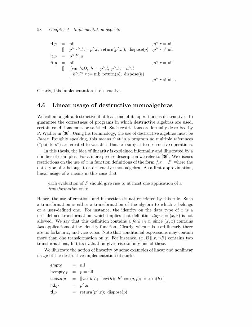
58 Chapter 4 Implementation aspects
tl.p = nil , p∧.r = nilp∧.r∧.l := p∧.l; return(p∧.r); dispose(p) , p∧.r 6= nil
lt.p = p∧.l∧.a
ft.p = nil , p∧.r = nil|[var h:D; h := p∧.l; p∧.l := h∧.l; h∧.l∧.r := nil; return(p); dispose(h)]| , p∧.r 6= nil .
Clearly, this implementation is destructive.
4.6 Linear usage of destructive monoalgebras
We call an algebra destructive if at least one of its operations is destructive. Toguarantee the correctness of programs in which destructive algebras are used,certain conditions must be satisfied. Such restrictions are formally described byP. Wadler in [36]. Using his terminology, the use of destructive algebras must belinear. Roughly speaking, this means that in a program no multiple references(“pointers”) are created to variables that are subject to destructive operations.
In this thesis, the idea of linearity is explained informally and illustrated by anumber of examples. For a more precise description we refer to [36]. We discussrestrictions on the use of x in function definitions of the form f.x = F , where thedata type of x belongs to a destructive monoalgebra. As a first approximation,linear usage of x means in this case that
each evaluation of F should give rise to at most one application of atransformation on x.
Hence, the use of creations and inspections is not restricted by this rule. Sucha transformation is either a transformation of the algebra to which x belongsor a user-defined one. For instance, the identity on the data type of x is auser-defined transformation, which implies that definition dup.x = (x, x) is notallowed. We say that this definition contains a fork in x, since (x, x) containstwo applications of the identity function. Clearly, when x is used linearly thereare no forks in x, and vice versa. Note that conditional expressions may containmore than one transformation on x. For instance, (x,B x,¬B) contains twotransformations, but its evaluation gives rise to only one of these.
We illustrate the notion of linearity by some examples of linear and nonlinearusage of the destructive implementation of stacks:
empty = nilisempty.p = p = nilcons.a.p = |[var h:L; new(h); h∧ := 〈a, p〉; return(h) ]|hd.p = p∧.a
tl.p = return(p∧.r); dispose(p).

4.6 Linear usage of destructive monoalgebras 59
Clearly, the use of tl must be restricted because it is destructive. The use ofthe other transformation cons is also restricted because evaluation of cons.a.pcreates an extra reference to p (and to a). There are no restrictions for creationempty and inspections isempty and hd.
To show how these operations can be used in a correct way, we consider theprogram:
f1.p = cons.(hd.p).(tl.p).
Exploiting the fact that eager evaluation does not prescribe the order in whichthe arguments of cons are to be evaluated, hd.p can be evaluated before tl.p.Hence, there exists a safe evaluation order so that execution of this programindeed establishes [[f1.p]] = [[p]]—as desired. Since tl.p destroys p, function f1 isalso destructive.
A safe evaluation order does not exist when two or more destructive opera-tions are to be performed on the same variable, as in
f2.p = cons.(hd.p).(cons.(hd.(tl.p)).(tl.(tl.p))).
Evaluation of either the first or the second occurrence of tl.p destroys p, hencethe remaining occurrence cannot be evaluated anymore; this definition containsa fork in p. Since, in this case, the same destructive operation is applied to p,the fork can be removed using a where-clause:
f3.p = cons.(hd.p).(cons.(hd.q).(tl.q)) |[ q = tl.p ]|.
To show that it is necessary to bound the number of transformations in theright-hand side of a function definition rather than the number of destructiveoperations, we consider:
f4.p = (tl.p, cons.a.p).
In this case, evaluation of tl.p destroys p, hence also cons.a.p is mutilated. Theproblem is that transformation cons.a.p creates an extra reference to p, andtherefore its use is also restricted.
The necessity of restricting transformations other than tl and cons as well,follows from the following refinement of f4:
f5.p = (tl.q, cons.a.r) |[ (q, r) = (p, p) ]|.
In this definition no stack-operations are applied to p. Nevertheless, evaluationof f5.p does not yield the desired result. The problem is that p is duplicated inthe where-clause by means of two applications of the identity function. Anotherexample of this phenomenon is
f6.p = (tl.q, cons.a.p) |[ q = p ]|.
This definition also contains a fork in p.

60 Chapter 4 Implementation aspects
Remark 4.2To obtain programs without forks for the above functions, duplication can beprogrammed as follows:
dup.p = (empty, empty) , isempty.p(cons.(hd.p).q, cons.(hd.p).r)|[ (q, r) = dup.(tl.p) ]| ,¬isempty.p.
This operation is a destructive transformation, hence its usage must be restrictedas well.
Another approach is to define operation copy which refines the identity on[T ]:
copy.p = nil , p = nil|[var h:L;; new(h); h∧ := 〈p∧.a, copy.(p∧.r)〉; return(h)]| , p 6= nil.
The use of copy need not be restricted because the value of p is merely inspected,not altered. In other words, although the type of this operation is LyL, copyshould not be considered as a transformation, but as an inspection followed bya creation. Note that copy cannot be programmed nondestructively in terms ofstack operations because tl is destructive.2
Finally, we present two examples involving conditional expressions. As arule, transformations should not be used in guards of conditional expressions,but guarded expressions may contain one transformation per variable each.
Example 4.3The following program for list reversal is nondestructive when the nondestructiveimplementation of stacks is used:
rev.x = h.x.[ ]|[ h.x.y = y , isempty.x
h.(tl.x).(cons.(hd.x).y) ,¬isempty.x]|.
However, since both x and y are used in a linear fashion in the definition of h, thisprogram also allows for the use of a destructive implementation of stacks. Thisyields a destructive implementation of list reversal, which is in fact an in-situimplementation, since the cell disposed by tl can be recycled by the operationnew invoked by cons.2
Example 4.4Let 1 denote the operator that merges two ascending lists of integers into asingle ascending list. With this operator at our disposal we can write a versionof mergesort that uses linear recursion only:

4.7 Benevolent side-effects 61
Mergesort = g f|[ f.[ ] = emptyf.(a` s) = snoc.(f.s).[a]g.x = [ ] , isempty.x
( hd.x , isempty.yg.(snoc.(tl.y).(hd.x1 hd.y)) ,¬isempty.y
) |[ y = tl.x ]| ,¬isempty.x]|.
To allow for the use of a destructive implementation of queues, variable y hasbeen introduced to see to it that x is used in a linear way. Note that function fcreates a queue and that g destructively inspects a queue.2
The last example shows that our rule for linear usage is not adequate in general,since it does not restrict the use of inspection g, although it is destructive. Abetter rule for a definition f.x = F seems to be that evaluation of F gives riseto at most one application of a transformation or a destructive inspection to x.This is however a little bit too restrictive, as we shall see in the next section.
4.7 Benevolent side-effects
Crucial to the efficiency of some data structures is that inspections “rearrange”their argument so that later operations take less time. These rearrangementsare harmless in the sense that the abstract value represented by the argumentremains the same. Such inspections are said to have benevolent side-effects [16].
As a somewhat contrived example of such an inspection, we consider thefollowing version of stack-operation hd:
hd.p = return(p∧.a); |[var h:L; new(h); h∧ := p∧; dispose(p); p := h ]|.
Note that the value of p is altered by hd.p, but that the value of [[p]] remainsintact. A possible advantage of this version of hd is that by selection of anappropriate cell by new(h), the cells in use can be kept in a more contiguous partof memory. In Part II we will encounter more appealing examples of inspectionswith benevolent side-effects (e.g., operation member in Section 11.2.1 on splaytrees).
To discuss the correctness of inspections with side-effects, we associate witheach inspection g ∈ C → T a function g′ ∈ C → T×C such that g′.c = (g.c, d),where d equals the value of c after evaluation of g.c. With the correspondingabstract inspection f ∈ A → T we associate function f ′ ∈ A → T×A withf ′.a = (f.a, a). Then f is said to be data-refined by g under coupling ' whenf ′ is data-refined by g′ under coupling '. Hence, an inspection with benevolentside-effects is a mixture of an inspection and a transformation.

62 Chapter 4 Implementation aspects
Since inspections with benevolent side-effects do not alter the abstract valueof their argument, they can be treated as nondestructive inspections. In sum-mary, we thus have the following restriction on the usage of a parameter thatbelongs to a destructive algebra.
For a function definition of the form f.x = F , x is said to be used ina linear fashion when each evaluation of F gives rise to at most oneapplication of a transformation or a destructive inspection to x, notcounting inspections with benevolent side-effects.
As before, this rule refers to transformations and inspections that are eitheroperations of the algebra or user-defined functions.

63
Chapter 5
Analysis of functionalprograms and algebras
As programs are designed in a modular way, we wish to analyze them in amodular way as well. In particular, we want to determine the complexity ofa program from the complexities of the operations of the algebras used in theprogram. For instance, given the complexities of zero and suc, we want to deter-mine the complexity of sucn.zero as a function of n. We call this a compositionalway of analyzing programs, which—in essence—means that the complexity of acomposition g f , say, can be expressed in terms of the complexities of f and g.
Since it is often difficult—or even infeasible—to determine the exact com-plexity of a program, it is customary to work with approximations. Traditionally,worst-case bounds are used for this purpose, but this approach does not givesatisfactory results in all circumstances: the worst-case complexity of g f maybe considerably “better” than the sum of the worst-case complexities of f andg. In other words, worst-case complexity is not compositional. As explainedin Chapter 3, we will therefore use amortized costs instead of actual costs todescribe the efficiency of implementations of algebras.
To guarantee that the amortized cost of a program is the sum of the amor-tized costs of the operations used by it, the corresponding algebras should beused linearly—in the same way as destructive algebras should be used linearly toguarantee the correctness of a program. This connection between destructivityand amortization leads to interesting trade-offs, as will be shown at the end ofthis chapter.
5.1 Cost measures
As explained in Section 4.2, execution of a functional program f on an inputx boils down to the reduction of expression f.x. Such a reduction requirestime as well as space and it is the goal of an analysis to quantify the use ofthese resources. More concretely, the goal of an analysis of a program f is to

64 Chapter 5 Analysis of functional programs and algebras
express, as a function of x, the cost of evaluating f.x. Here, the cost dependson the choice of a cost measure, which is chosen beforehand. Since execution offunctional programs amounts to the reduction of expressions, our cost measureswill be mappings from expressions to the real numbers.
There are two—usually conflicting—demands that determine the suitabilityof a cost measure: it should be realistic for the intended purpose, and it should bemanageable, i.e., not overly complicated. For instance, cost measure N , definedby N (E)=“the total number of unfoldings needed to evaluate E”, is in generala realistic measure but often much too complicated. For a sorting program, ameasure like “the number of comparisons needed to evaluate E” is probablymore suitable; this measure counts the number of unfoldings of the predefinedoperation <, say.
Once a suitable cost measure has been defined, the program can be analyzed.We want to do so by analyzing the auxiliary functions, which constitute theprogram, one at a time. To support such a modular analysis, we introduce the“cost of a function”.
Definition 5.1A cost measure is a mapping from expressions to the real numbers. For a func-tional program f , the cost of f with respect to cost measure T is the mappingT [f ] defined by
T [f ](E) = T (f.E)− T (E),
for E ∈ dom f .2
The important property of mapping T [·] is that it satisfies the compositionrule, which enables us to decompose the analysis of compositions like g f .
Property 5.2 (composition rule for T [·])If T ((g f).E) = T (g.(f.E)), then
T [g f ](E) = T [f ](E) + T [g](f.E).
ProofT [g f ](E)
= Definition 5.1 T ((g f).E)− T (E)
= above proviso T (g.(f.E))− T (E)
= arithmetic T (g.(f.E))− T (f.E) + T (f.E)− T (E)
= Definition 5.1 T [g](f.E) + T [f ](E).
2

5.1 Cost measures 65
The proviso in this property is rather weak; it is satisfied by all cost measuresthat we use for our programs. This has to do with the fact that we use asan abbreviation mechanism only, and therefore we do not want that expressions(g f).E and g.(f.E) are distinguished by our cost measures. Fancy cost mea-sures that do not satisfy this proviso, such as “the length of expression E” or“the number of occurrences of in E”, will not be used.
At first sight one might think that another property of T [f ] is that T [f ](E)depends on the value of E only, not on the shape of E, but this is not truein general. Take, for instance, cost measure S defined by S(E)=“the maximalamount of storage space in use during the evaluation of E”. Since the maximalamount of storage space in use during the evaluation of f.E is either in usebefore f is unfolded, in which case S(f.E) = S(E), or only after f has beenunfolded, in which case S(f.E) > S(E), we observe that S[f ](E) may be zeroas well as positive, depending on the shape of E.
In the sequel, however, we will concentrate on cost measures that are relatedto the amount of time required for the evaluation of expressions. We call thesedistributive cost measures. The class of distributive cost measures will not bedefined explicitly: we only postulate some distribution rules which are satisfiedby such cost measures.
One of the most important distribution rules for a cost measure T is thatfor a function definition of the form f.x = F :
T (f.E) = T (E) + Cf (val(E)) + T (F xval(E)),
where val(E) denotes the value of E, and Cf ∈ dom f→Real describes the actualcost of unfolding f ’s definition for each possible value. Since eager evaluation off.E amounts to the evaluation of E, followed by the unfolding of f ’s definition,which in turn gives rise to the evaluation of F with x replaced by the valueof E (cf. Section 4.2), we see that the cost of f.E equals the sum of the costsof these three phases for distributive cost measures. Hence, the value of E iscomputed only once and shared by all occurrences of x in F . A consequence ofthis distribution rule is that
T [f ](E) = T [f ](val(E)),
since val(val(E)) = val(E).
In the applications in Part II, all cost measures count unfoldings of (usu-ally recursive) user-defined functions and/or unfoldings of predefined operations.Since we assume that our programs are executed according to the eager evalu-ation scheme (Section 4.2), these cost measures enjoy some nice distributivityproperties. Below, we will present these properties for an extreme member ofthis class, viz. the previously introduced cost measure N , which counts all un-foldings of predefined operations and user-defined functions.

66 Chapter 5 Analysis of functional programs and algebras
Distribution rules for N
1. The first rule is an instance of the above distribution rule for T (f.E),where f is defined by f.x = F :
N (f.E) = N (E) + 1 +N (F xval(E)).
2. With respect to , we have (cf. Property 5.2):
N ((g f).E) = N (g.(f.E)).
3. For conditional expressions the following rule is appropriate:
N ((E,B F,¬B)) = N (B) +
N (E) , BN (F ) ,¬B,
which expresses that in case of complementary guards, only one of theseis evaluated, and that, subsequently, only the relevant expression is evalu-ated.
4. As for where-clauses, we consider expressions of the form F |[x = E]|. Theseare reduced in the same way as f.E is reduced. Hence:
N (F |[x = E]|) = N (E) + 1 +N (F xval(E)).
5. Another simple rule is that for a predefined binary operator ⊕, say, wehave
N (E ⊕ F ) = N (E) +N (F ) + 1,
which reflects the fact that N counts unfoldings of predefined operations.
6. In connection with the use of patterns in the left-hand sides of functiondefinitions, we consider a definition of the form
f.[ ] = F
f.(a` s) = G.
For this definition we have the property that
N (f.E) = N (E)+1+1+
N (F ) , E = [ ]1+1+N (Ga,s
val(hd.E),val(tl.E)) , E 6= [ ].
It may be interpreted as follows: first E is evaluated and it is determinedwhether E is empty or not, which requires one unfolding of (=[ ]). Sub-sequently f ’s definition is unfolded, which gives rise to evaluation of F orto evaluation of G with a and s replaced by the values of hd.E and tl.E.The latter case requires one unfolding of hd and one of tl.

5.2 Worst-case analysis 67
7. Finally, there is the trivial but useful property that evaluation of an ex-pression terminates as soon as it has been reduced to its value, which isreflected by the rule
N (val(E)) = 0.
These rules hold for all cost measures T that count unfoldings of user-definedand/or predefined functions, except that the “+1 terms” in the equations forT (f.E), T (E ⊕ F ), and T (F |[x = E]|) are absent for those unfoldings that arenot counted by T .
To facilitate the definition of distributive cost measures, we use dots on topof the =-signs in function definitions to mark the unfoldings that are countedby the measure. In case a function definition consists of several alternatives thedot marks all the alternatives. For example, the cost measure T defined by
bubble.[ ] = [ ]bubble.[a] = [a]bubble.(a` b` s) .= a` bubble.(b` s) , a ≤ b
b` a` bubble.s , a > b
satisfies T (E)=“the number of unfoldings of the recursive alternative of bubbleneeded to evaluate E”, and also T (E)=“the number of unfoldings of ≤ (or >)needed to evaluate E”.
The distribution rules for T enable us to derive relations for T [f ] that followthe structure of the definition of f . In case f ’s definition is recursive, this givesrise to recurrence relations for T [f ]. For example, using Definition 5.1, we haveas recurrence relation for T [bubble]:
T [bubble]([ ]) = 0T [bubble]([a]) = 0
T [bubble](a` b` s) = 1 +
T [bubble](b` s) , a ≤ bT [bubble](s) , a > b.
Using the distribution rules, this recurrence relation may actually be derived, butthis is too laborious and therefore omitted. Note that it suffices to investigateT [bubble](s) for all values s because T is distributive.
5.2 Worst-case analysis
It seems that we have already reached our goal now that we have introduced T [·],since it satisfies some nice composition and distribution properties when T isdistributive. Unfortunately, however, an explicit formula for T [f ] cannot alwaysbe given, and in such a case we must content ourselves with approximations ofT [f ]. A common method of approximating the cost of a function f is to useupper bounds for T [f ](x) that depend on the “size” of x only. In these so-called

68 Chapter 5 Analysis of functional programs and algebras
worst-case analyses, the input values are partitioned into classes of equal-sizedinputs, and the worst-case complexity of a function f is then determined for eachpossible size N . That is, with #x denoting the size of x,
(Maxx : x ∈ dom f ∧ #x = N : T [f ](x))
is determined as a function of N . For program bubble, for example, the worstcase occurs when s is ascending; the solution of the recurrence relation then isT [bubble](s) = (#s−1) max 0.
In many cases it is even too complicated to find an explicit formula for theworst-case complexity. Instead of an exact formula we then give an upper boundlike #s for T [bubble](s), or we simply say that T [bubble](s) is O(#s) when we areonly interested in the asymptotic cost. The problem with such approximationsis that they are not compositional in the sense that a tight upper bound for theworst-case complexity of T [g f ] cannot be obtained from tight upper boundsfor the worst-case complexities of T [f ] and T [g]. This is illustrated by the nextexample.
Example 5.3We analyze a binary implementation of (Nat | 0, (+1) ). The concrete data typeis [0, 1] and the concrete operations are
zero.= [ ]
suc.[ ] .= [1]suc.(0` s) .= 1` ssuc.(1` s) .= 0` suc.s.
The cost measure defined by the dots is called T , which could also be done inwords by T (E)=“the number of unfoldings of zero and suc needed to evaluateE”. Our goal is to derive a tight bound for T [sucn.zero] as a function of n.
To this end we first analyze zero and suc in isolation. Clearly, T [zero] = 1,and for T [suc] we have the following recurrence relation:
T [suc]([ ]) = 1T [suc](0` s) = 1T [suc](1` s) = 1 + T [suc](s).
A tight upper bound for T [suc](s) in terms of #s thus is 1+#s.Repeatedly applying the composition rule for T [·] yields
T [sucn.zero] = T [zero] + (Σ i : 0 ≤ i < n : T [suc](suci.zero)).
In order to use the upper bound for T [suc], we observe that list suci.zero haslength at most 1+log2(i+1). Therefore T [suc](suci.zero) is at most 2+log2(i+1),and we obtain an O(n log n) bound for T [sucn.zero].
However, T [sucn.zero] is O(n), as will be shown in Example 5.7; the fact thatT [suc](s) ≤ #s (and that this bound is tight) cannot be used to prove this.2

5.3 Amortized cost of functions 69
5.3 Amortized cost of functions
Suppose that our goal is to determine the worst-case complexity of fn as afunction of n. As demonstrated in Example 5.3, the worst-case complexityof f does not, in general, provide a clue to the worst-case complexity of fn.Instead, we will use amortized costs for f and fn, which are defined in termsof a potential function. In the functional setting, a potential function is—like acost measure—a mapping on expressions. Unlike a cost measure, however, thepotential of an expression depends on its value only, not on the way in whichthis value is expressed. This corresponds to the idea behind potential functionsin Chapter 3: in the imperative setting, a potential function depends on thevalue of the state only, not on how the state has been reached.
Definition 5.4A potential function Φ is a mapping from expressions to the real numbers satis-fying
Φ.E = Φ.val(E).
The amortized cost of f with respect to cost measure T and potential Φ is themapping A[f ] defined by
A[f ](E) = T [f ](E) + Φ.(f.E)− Φ.E,
for E ∈ dom f .2
In an amortized analysis, the potential function is defined for the relevant valuesonly, e.g., for the data type of an algebra. For other values, the definition of thepotential is extended in a straightforward way. In connection with the use oftuples, for example, the potential of the empty tuple ⊥ is usually defined equalto 0. For constant f , Definition 5.4 then yields
A[f ] = T [f ] + Φ.f .
Also, in connection with the use of pairs, Φ.(E,F ) is usually defined equal tothe sum of Φ.E and Φ.F , so that
A[f ]((E,F )) = T [f ]((E,F )) + Φ.(f.E.F )− Φ.E − Φ.F
for functions f on pairs.Since Φ.E = Φ.val(E), A[·] inherits a number of properties of T [·]. For
instance, the composition rule is inherited.
Property 5.5 (composition rule for A[·])If
T [g f ](E) = T [f ](E) + T [g](f.E),

70 Chapter 5 Analysis of functional programs and algebras
then also
A[g f ](E) = A[f ](E) +A[g](f.E).
Proof
A[g f ](E)
= Definition 5.4 T [g f ](E) + Φ.((g f).E)− Φ.E
= above proviso and restriction on Φ in Definition 5.4 T [f ](E) + T [g](f.E) + Φ.(g.(f.E))− Φ.E
= arithmetic T [g](f.E) + Φ.(g.(f.E))− Φ.(f.E) + T [f ](E) + Φ.(f.E)− Φ.E
= Definition 5.4 A[g](f.E) +A[f ](E).
2
Also “independence of the shape of E” is inherited by A[f ](E).
Property 5.6If T [f ](E) = T [f ](val(E)), then A[f ](E) = A[f ](val(E)) as well.2
There is however a crucial difference between A[·] and T [·]. To discuss thisdifference, we introduce cost measure A:
A(E) = T (E) + Φ.E.
Then the amortized cost of f w.r.t. T and Φ (cf. Definition 5.4) equals the cost off w.r.t. A (cf. Definition 5.1). Since A inherits the common properties of T andΦ, Properties 5.5 and 5.6 are readily seen to be valid. However, distributivityof T does not imply distributivity of A because Φ is not distributive!
Now, since T is usually distributive, it is not difficult to obtain a relationfor T [f ] based on the structure of f ’s definition. But A is not distributive, andtherefore a relation for A[f ] cannot be obtained in general by substituting A forT in the relation for T [f ]. Consider, for instance, function dup defined by
dup.x.= (x, x).
Assuming that T is distributive and that Φ distributes over pairs, hence that Adistributes over pairs (i.e., A((x, y)) = A(x) +A(y)), we observe for value x:

5.4 Amortized analysis 71
T [dup](x)= Definition 5.1
T (dup.x)− T (x)= definition dup
1 + T ((x, x))− T (x)= T is distributive
1 + T (x) + T (x)− T (x)= T (x) = 0
1,
A[dup](x)= Definition 5.1
A(dup.x)−A(x)= definition dup
1 +A((x, x))−A(x)= A distributes over pairs
1 +A(x) +A(x)−A(x)= T (x) = 0, hence A(x) = Φ.x
1 + Φ.x.
Hence, T [dup](x) = 1 but A[dup](x) = 1+Φ.x. Similarly, when x is tripled, thedifference becomes 2Φ.x, and so on. On the other hand, for function sink, withsink.x
.= ⊥, we have that T [sink](x) = 1 and A[sink](x) = 1− Φ.x.In general, for a definition of the form f.x = F , there will be no difference
between the relations for A[f ] and T [f ] when x occurs exactly once in F (andT is distributive). This is reflected by the difference between
T [f ](E) = Cf (val(E)) + T (F xval(E)),
and
A[f ](E) = Cf (val(E)) +A(F xval(E))− Φ.E.
(Note that the equality for T [f ](E) implies the equality for A[f ](E).) To rewriteT (F x
val(E)) into a formula in terms of T [·], as many terms T (val(E)) can be usedas necessary (since T (val(E)) = 0), but to rewrite A(F x
val(E)) into a formula interms of A[·], only a single term Φ.E is available.
In Section 5.5 we will present a simple method to ensure that the relationsfor T [·] are inherited by A[·].
5.4 Amortized analysis
Consider a function f for which rng f ⊆ dom f . Suppose that the worst-casecomplexity of fn (as a function of n) cannot be determined from the worst-case complexity of f . Then we perform an amortized analysis, which typicallyproceeds as follows. For the sake of convenience we assume that #(f.x) = #x.
Having defined cost measure T , our aim is to bound T [fn](x) in terms of#x and n. To this end we repeatedly apply the composition rule for A[·] (Prop-erty 5.5) to A[fn], where
A[fn](x) = T [fn](x) + Φ.(fn.x)− Φ.x.
This yields the following equation:

72 Chapter 5 Analysis of functional programs and algebras
T [fn](x) = (Σ i : 0 ≤ i < n : A[f ](f i.x)) + Φ.x− Φ.(fn.x),(1)
from which we obtain a tight bound for T [fn](x) by choosing a suitable potentialΦ. But, just as it is difficult to find an explicit formula for T [f ](x), it is, ingeneral, difficult to find an explicit formula for A[f ](x). Therefore, we use theworst-case approximation of A[f ] by considering the following bound for T [fn]derived from (1), using that #(f.x) = #x:
T [fn](x) ≤ n ∗ (Max y : #y = #x : A[f ](y)) + Φ.x− Φ.(fn.x).
The object is now to choose Φ such that (Max y : #y=#x : A[f ](y)) is min-imized, thereby keeping in mind that Φ.x − Φ.(fn.x) may not be too large aswell.
As for the latter requirement on Φ, it is often convenient to choose a non-negative function for Φ. The above upper bound then simplifies to
T [fn](x) ≤ n ∗ (Max y : #y = #x : A[f ](y)) + Φ.x.
By keeping Φ.x small with respect to #x, a tight upper bound for T [fn](x) interms of #x is obtained.
This above method of amortized analysis is applied in the next example toimprove the analysis of sucn.zero in Example 5.3.
Example 5.7 (see Example 5.3)The amortized costs for zero and suc are
A[zero] = T [zero] + Φ.zero
A[suc](s) = T [suc](s) + Φ.(suc.s)− Φ.s,
where Φ ∈ [0, 1]→Real is the potential function. Since
A[sucn.zero] = T [sucn.zero] + Φ.(sucn.zero),
the composition rule for A[·] yields
T [sucn.zero] = A[zero] + (Σ i : 0≤i<n : A[suc](suci.zero))− Φ.(sucn.zero).
This equality yields an O(n) bound for T [sucn.zero] provided Φ is nonnegative,and A[zero] and A[suc](s) are both constant.
By definition, we have that A[zero] = 1 + Φ.[ ], hence constant. To keepA[zero] small and Φ nonnegative, we take Φ.[ ] = 0. Then A[zero] = 1.
Similarly, we have that A[suc]([ ]) is O(1), independent of the definition of Φ.To derive a suitable definition for Φ, we first observe for the second alternativeof suc:

5.4 Amortized analysis 73
A[suc](0` s)= definition of A[suc]
T [suc](0` s) + Φ.(suc.(0` s))− Φ.(0` s)= recurrence relation for T [suc], definition of suc
1 + Φ.(1` s)− Φ.(0` s)= simplify by choosing Φ.(b` s) = ϕ.b+ Φ.s
1 + ϕ.1− ϕ.0.
By the introduction of ϕ, A[suc](0` s) becomes independent of s, hence O(1).To obtain a suitable definition for ϕ we proceed with the last alternative of suc:
A[suc](1` s)= definition of A[suc]
T [suc](1` s) + Φ.(suc.(1` s))− Φ.(1` s)= recurrence relation for T [suc], definition of suc
1 + T [suc](s) + Φ.(0` suc.s)− Φ.(1` s)= definition of A[suc]
A[suc](s) + 1 + Φ.(0` suc.s)− Φ.(suc.s)− (Φ.(1` s)− Φ.s)= Φ.(b` s) = ϕ.b+ Φ.s, see previous derivation
A[suc](s) + 1 + ϕ.0− ϕ.1.
The term 1 + ϕ.0 − ϕ.1 may be interpreted as the amortized cost of unfoldingsuc.(1` s).
To ensure that A[suc] is O(1), ϕ should be chosen such that 1+ϕ.0−ϕ.1 ≤ 0.To obtain a nonnegative and small Φ, we take ϕ.0 = 0 and ϕ.1 = 1 (hence,1 + ϕ.0− ϕ.1 = 0). As potential we thus obtain:
Φ.[ ] = 0Φ.(b` s) = b+ Φ.s,
hence Φ.s equals the number of 1’s in s. From this definition for Φ, it follows byinduction that A[suc](s) = 2. The above equation for T [sucn.zero] then yields
T [sucn.zero] = 1 + 2n− Φ.(sucn.zero),
from which we conclude that T [sucn.zero] is O(n), since Φ is nonnegative. Weremark that the upper bound 1+2n is as good as tight (T [sucn.zero] = 2n whenn is a power of two).2
In this example, the potential has been derived in a calculational way. In par-ticular, the fact that ϕ.b = b is a suitable definition directly follows from thederivation. The systematic derivation of potential functions is an importanttopic in the case-studies of Part II.

74 Chapter 5 Analysis of functional programs and algebras
5.5 Amortization and linearity
At this point it should be clear that worst-case amortized complexities shouldbe used instead of worst-case actual complexities as a general way to describethe efficiency of implementations of algebras. But, as explained at the end ofSection 5.3, a problem with the use of amortized costs is that for a function defi-nition of the form f.c = F , say, the relations for T [f ] are not necessarily inheritedby A[f ]. Recall, for example, that A[dup](c) = 1 + Φ.c whereas T [dup](c) = 1for dup.c .= (c, c). To achieve that the relations for T [f ] are indeed inheritedby A[f ] some restrictions must be imposed on expression F . Below we will de-scribe these restrictions under the assumption that A[·] is defined according tothe following scheme.
Let C be a (concrete) monoalgebra with data type C. Let T denote a costmeasure for the programs of C, and let Φ be a potential function defined onC. In accordance with Definition 5.4, the amortized costs of creations andtransformations are defined as follows.
(a) For a creation g of type T → C:
A[g](x) = T [g](x) + Φ.(g.x).
(b) For a transformation g of type C×CyC:
A[g](c, d) = T [g](c, d) + Φ.(g.c.d)− Φ.c− Φ.d.
To obtain (a) as instantiation of Definition 5.4, we take Φ.x = 0 for x ∈ T . Doingthe same for inspections, however, yields a not so useful definition. Instead, wedistinguish two types of inspections.
(c) For an inspection g of type C → T :
(i) A[g](c) = T [g](c), or(ii) A[g](c) = T [g](c)− Φ.c.
Here, (ii) can be obtained as instantiation of Definition 5.4, again with Φ.x = 0for x ∈ T . In most cases, however, (i) is the appropriate definition for A[g]:defining A[g](c) = T [g](c) means that the costs of inspections are not amortized.
If A[·] is defined according to the above scheme, the restriction on f.c = Fis that each evaluation of F should give rise to at most one application to c ofa transformation or an inspection of type (ii). In that case, A[f ] inherits therelations for T [f ]. Note that the use of inspections of type (i) is not restricted bythis rule. This is essential because inspections are typically used in combinationwith a transformation, and this would be impossible when the potential playeda role in the amortized costs of both.
Inspections are allowed to have benevolent side-effects. In that case thepotential of cmay be altered by the evaluation of g.c, and this change in potential

5.6 Purely-functional deques 75
may be necessary to amortize the cost of g. To analyze such an inspection, weconsider function g′ ∈ C → T×C with g′.c = (g.c, d), where d equals the valueof c after evaluation of g.c (cf. Section 4.7). The amortized costs of g′ are definedas follows:
A[g′](c) = T [g](c) + Φ.d− Φ.c.
In Part II we will see some examples of inspections with benevolent side-effectsthat are efficient in the amortized sense only (e.g., operation member in Sec-tion 11.2.1 on splay trees). In the above rule, such an inspection may be treatedas an inspection of type (i).
Calling an inspection of type (i) a nondestructive inspection and an inspec-tion of type (ii) a destructive one, the restriction on f.c = F coincides with thenotion of linearity defined at the end of Chapter 4. Therefore we shall say thatan algebra which is efficient in the amortized sense only must be restricted tolinear usage in order to ensure that the amortized costs add up in the same wayas the actual costs. An important observation is now that an algebra which iseither destructive or efficient in the amortized sense only might as well be both.This leads to interesting trade-offs, as we will show in the next section.
5.6 Purely-functional deques
In Chapter 7 of his Ph.D. thesis [17] Hoogerwoord derives an efficient implemen-tation for a symmetric set of list operations. The idea behind his design is basedon an efficient implementation of queues in LISP (see e.g. [13, pp. 250–251]). Inthis section, we first cast this design in our style, after which we go on to ex-periment with the amortized analysis of more advanced operations programmedin terms of the symmetric list operations. In this way we gain some experiencewith the computation of the amortized costs of composite functions from theamortized costs of the constituent parts.
5.6.1 Specification and implementation
Using the algebra of stacks
S = ( [T ] | [ ], (=[ ]), ` , hd, tl ),
whose operations all have O(1) actual cost, we present an implementation of thealgebra of deques (“double-ended queues”)
DQ = ( [T ] | [ ], (=[ ]), ` , hd, tl, a , lt, ft, rev ),
with signature
S2 = (X | empty, isempty, cons, hd, tl, snoc, lt, ft, rev ),

76 Chapter 5 Analysis of functional programs and algebras
such that all operations of S2 have O(1) amortized cost. Apart from the symmet-rical counterparts of the last three operations of S, we have included operationrev, because any program for rev in terms of the other operations of DQ isbound to be linear, while it is a simple O(1) operation in the representationused for [T ] below. Hence, rev cannot be programmed without loss of efficiencyin terms of the other operations of DQ.
The definition of S2 is as follows (see [17] for a solid derivation). Set Xis a subset of [T ]×[T ] and S2 refines DQ under abstraction [[·]] with [[〈s, t〉]] =s++ rev.t. To allow for an efficient implementation of hd and lt, set X is definedas follows:
X = 〈s, t〉 | (s = [ ] ⇒ #t ≤ 1) ∧ (t = [ ] ⇒ #s ≤ 1).
Using the operations of S, the operations of S2 are programmed as follows:
empty = 〈[ ], [ ]〉
isempty.〈s, t〉 = s = [ ] ∧ t = [ ]
cons.a.〈s, t〉 = 〈a` s, t〉 , t 6= [ ]〈[a], s〉 , t = [ ]
hd.〈s, t〉 = hd.s , s 6= [ ]hd.t , s = [ ]
tl.〈s, t〉 = 〈[ ], [ ]〉 ,#s = 0〈rev.(t↓k), t↑k〉 |[ k = #t div 2 ]| ,#s = 1〈tl.s, t〉 ,#s ≥ 2
snoc.〈s, t〉.a = 〈s, a` t〉 , s 6= [ ]〈t, [a]〉 , s = [ ]
lt.〈s, t〉 = hd.t , t 6= [ ]hd.s , t = [ ]
ft.〈s, t〉 = 〈[ ], [ ]〉 ,#t = 0〈s↑k, rev.(s↓k)〉 |[ k = #sdiv 2 ]| ,#t = 1〈s, tl.t〉 ,#t ≥ 2
rev.〈s, t〉 = 〈t, s〉 .
In the programs for tl and ft some list operations are used which are not providedby algebra S. We assume that these operations are implemented in terms of theoperations of S such that rev.s and #s take O(#s) time, and, s↑n and s↓n takeO(n) time—as usual. Furthermore, an expression like #s≥2 is just short fors6= [ ] cand tl.s6=[ ], so it takes only O(1) time to evaluate it.

5.6 Purely-functional deques 77
Now, note that all operations are O(1), except that evaluation of tl.〈s, t〉 takesO(#t) time in case #s=1 (and similarly for ft). Therefore we count 1+#t unitsfor such an unfolding of tl, 1+#s time units for the corresponding unfoldingof ft, and in all other cases we just count one time unit per unfolding of anoperation of S2. This defines cost measure T . The potential function is definedas Φ.〈s, t〉 = |#s−#t|, and the amortized costs of the operations are all O(1),with (cf. scheme in Section 5.5):
A[empty] = T [empty] + Φ.empty
A[isempty](x) = T [isempty](x)A[cons](a, x) = T [cons](a, x) + Φ.(cons.a.x)− Φ.xA[hd](x) = T [hd](x)A[tl](x) = T [tl](x) + Φ.(tl.x)− Φ.xA[snoc](x, a) = T [snoc](x, a) + Φ.(snoc.x.a)− Φ.xA[lt](x) = T [lt](x)A[ft](x) = T [ft](x) + Φ.(ft.x)− Φ.xA[rev](x) = T [rev](x) + Φ.(rev.x)− Φ.x.
In the analyses in the next section, we shall use that Φ satisfies 0≤Φ.x≤#[[x]],for all x∈X.
To give an idea of how the correctness of the above results can be proved, weend this section with a treatment of case #s = 1 for tl.〈s, t〉. The correctness ofthe program for this case follows from 〈rev.(t↓k), t↑k〉 ∈ X (since k = #t div 2),and
[[tl.〈s, t〉]]= definition of tl
[[〈rev.(t↓k), t↑k〉]]= definition of [[·]] rev.(t↓k) ++ rev.(t↑k)
= property of rev; t↑k++ t↓k = t rev.t
= #s = 1 tl.(s++ rev.t)
= definition of [[·]] tl.[[〈s, t〉]].
The O(1) bound for the amortized cost follows from (using T [tl](〈s, t〉) = 1+#t):
A[tl](〈s, t〉)= definition of A[tl]
T [tl](〈s, t〉) + Φ.(tl.〈s, t〉)− Φ.〈s, t〉

78 Chapter 5 Analysis of functional programs and algebras
= definitions of T and tl 1 + #t+ |(#t− k)− k| − |1−#t|
≤ arithmetic (k = #t div 2) 1 + #t+ #tmod2 + 1−#t
≤ arithmetic 3.
5.6.2 Some applications and their analyses
In this section we perform a series of amortized analyses of more complicatedlist operations. Each example emphasizes a particular issue of amortized anal-ysis. Given the choice for X in the previous section, all these operations areimplemented without loss of efficiency, so there is no need to add any of theseto the algebra of deques.
Catenation — a simple amortized analysis
For ++ we have as obvious refinement:
cat.x.y = y , isempty.xcat.(ft.x).(cons.(lt.x).y) ,¬isempty.x.
Since the costs of the operations of S2 dominate, we charge the cost of eachunfolding of cat to the applications of these operations. Thus, we leave thedefinition of T unchanged and define
A[cat](x, y) = T [cat](x, y) + Φ.(cat.x.y)− Φ.x− Φ.y,
since ++ is a transformation. Then the definition of cat is linear, so we have asrecurrence relation for A[cat]:
A[cat](x, y) =
A[isempty](x) , [[x]] = [ ]A[cat](ft.x, cons.(lt.x).y) +A[ft](x)+A[cons](lt.x, y) +A[lt](x) +A[isempty](x) , [[x]] 6= [ ],
from which we infer that A[cat](x, y) is O(#[[x]]).Of course, one can also design a program for cat.x.y with cost O(#[[y]]). By
choosing the cheapest program, we obtain an implementation of cat for whichcat.x.y takes O(#[[x]] min#[[y]]) time, provided that we see to it that #[[x]] and#[[y]] can be determined in O(1) time.
Length — introducing an auxiliary definition
Operation # may be refined by the following function:
len.x = 0 , isempty.x1 + len.(tl.x) ,¬isempty.x.

5.6 Purely-functional deques 79
Since # is an inspection operation, we define:
A[len](x) = T [len](x).
However, in order to analyze len, we introduce the following auxiliary definition:
A′[len](x) = T [len](x)− Φ.x,
for which we have the following recurrence relation:
A′[len](x) =
A[isempty](x)− Φ.x , [[x]] = [ ]A′[len](tl.x) +A[tl](x) +A[isempty](x) , [[x]] 6= [ ].
Since Φ.x ≥ 0, it follows that A′[len](x) is O(#[[x]]), and, since Φ.x ≤ #[[x]], wehave that A[len](x) is O(#[[x]]) as well.
From the above analysis we conclude that it is sometimes necessary to in-troduce a different definition for the amortized cost of an operation in order toperform the analysis of its program. In this case we need the term −Φ.x inthe definition of A′[len](x) to amortize the cost of the applications of tl in therecursive alternative of len. Subsequently, the bounds for Φ enabled us to derivea bound for A[len](x).
Take and drop — extending the definition of T
For ↑ (“take”) and ↓ (“drop”) we have as refinements
take.x.0 = emptytake.x.(n+1) = cons.(hd.x).(take.(tl.x).n),
and
drop.x.0 = xdrop.x.(n+1) = drop.(tl.x).n.
With T as defined so far we have T [drop](x, 0) = 0, which is evidently notrealistic. Therefore, we extend the definition of T as follows: we count one unitper unfolding of the nonrecursive alternative of drop. The amortized costs ofthese transformations are
A[take](x, n) = T [take](x, n) + Φ.(take.x.n)− Φ.xA[drop](x, n) = T [drop](x, n) + Φ.(drop.x.n)− Φ.x.
A straightforward analysis gives O(n) bounds for the amortized costs of take.x.nand drop.x.n.

80 Chapter 5 Analysis of functional programs and algebras
Element selection — less efficient than expected?
We have elt.x.n as refinement for [[x]].n, where
elt.x.0 = hd.xelt.x.(n+1) = elt.(tl.x).n.
Operation elt is an inspection, hence
A[elt](x, n) = T [elt](x, n).
In order to amortize the cost of the applications of tl, we introduce the followingauxiliary definition:
A′[elt](x, n) = T [elt](x, n)− Φ.x,
for which we have as recurrence relation:
A′[elt](x, 0) = A[hd](x)− Φ.xA′[elt](x, n+1) = A′[elt](tl.x, n) +A[tl](x).
Since Φ.x ≥ 0, A′[elt](x, n) is O(n), but for A[elt](x, n) we can only concludethat it is O(#[[x]]), using that Φ.x ≤ #[[x]]. Now, given the choice for X in theprevious section, this bound for A[elt](x, n) is tight; the worst case occurs whenthe second element of [[〈s, t〉]] is selected and #s = 1, or when the last but oneelement of [[〈s, t〉]] is selected and #t = 1. So, element selection for deques is notas efficient as for stacks.
Splitting lists — an avoidable fork
As a kind of inverse of cat we consider operation split, which splits a list into aprefix of specified length and the remaining suffix:
split.x.n = 〈take.x.n, drop.x.n〉.
Since split is a transformation with two outputs, we have
A[split](x, n) = T [split](x, n) + Φ.(split.x.n.0) + Φ.(split.x.n.1)− Φ.x.
Now recall that the definitions of A[take](x, n) and A[drop](x, n) both containterm −Φ.x, and observe that this term occurs only once in the definition ofA[split](x, n). This gives rise to a fork in x:
A[split](x, n) = A[take](x, n) +A[drop](x, n) + Φ.x.
Since Φ.x≤#[[x]], the best we can conclude from this relation is that A[split](x, n)is O(#[[x]]), using that A[take](x, n) and A[drop](x, n) are O(n). However, by

5.6 Purely-functional deques 81
tupling the programs for take and drop, we obtain an algorithmic refinement ofsplit for which A[split](x, n) can be shown to be O(n):
split.x.0 = 〈empty, x〉split.x.(n+1) = 〈cons.(hd.x).y, z〉 |[ 〈y, z〉 = split.(tl.x).n ]|.
As in the previous program, x occurs twice in the right-hand side of the secondalternative, but now only one transformation (viz. tl) is applied to it. Therefore,
A[split](x, 0) = A[empty]A[split](x, n+1) = A[split](tl.x, n) +A[hd](x) +A[tl](x)
+A[cons](hd.x, split.(tl.x).n.0),
which yields an O(n) bound for the amortized costs of this program for split.From this example we draw the important conclusion that it may be neces-
sary to consider a more detailed refinement of a program in order to avoid forks.In this case, we were able to avoid a fork, but in the next example we encountera situation in which we cannot.
List of all prefixes — unavoidable forks
Let function f , f ∈ X → [X], be defined by
f.x = [x] , isempty.xx` f.(ft.x) ,¬isempty.x.
Then f.x is the list of all prefixes of x (in decreasing order of length). Since ftransforms a deque into a list (more precisely, a stack) of deques, the amortizedcosts of f are defined as follows:
A[f ](x) = T [f ](x) + Φ∗.(f.x)− Φ.x,
with Φ∗.[ ] = 0 and Φ∗.(x`xs) = Φ.x + Φ∗.xs. Just as in the previous sectionthere is a fork in the recursive alternative of f , which gives rise to the term Φ.xin the following recurrence relation:
A[f ](x) =
A[isempty](x) , [[x]] = [ ]A[f ](ft.x) +A[ft](x) +A[isempty](x) + Φ.x , [[x]] 6= [ ].
Since Φ.x is at most #[[x]], it follows thatA[f ](x) isO((#[[x]])2). Now, in contrastwith the previous example, we cannot give an algorithmic refinement of f suchthat A[f ] is linear; we even conjecture that it is impossible to refine f such thatA[f ] is linear1. This result seems somewhat disappointing when one realizes
1As a motivation for this conjecture, we briefly describe a failing attempt of ours: we assumethat X and Φ are defined as in Hoogerwoord’s refinement. To achieve linearity of A[f ](x), weaim at linearity of T [f ](x) and Φ∗.(f.x). This suffices because Φ is nonnegative. A simple wayto establish linearity of Φ∗.(f.x) is to keep the Φ-values O(1) for all elements of f.x. This meansthat the two components of all elements of f.x should be roughly of equal length. Hence, f.xshould be a list of #[[x]]+1 “balanced pairs”. From a study of this list, we conclude that it isimpossible to generate it in linear time.

82 Chapter 5 Analysis of functional programs and algebras
that T [f ] itself is linear: with A′[f ](x) = T [f ](x)−Φ.x, we have that A′[f ](x) isO(#[[x]]), and, consequently, T [f ](x) is O(#[[x]]) (using Φ.x ≤ #[[x]]). However,as we will argue in Section 5.6.3, it is not so bad that A[f ] is quadratic.
Deque of all prefixes — nested deques
The following data refinement of f is also an instructive example:
g.x = cons.x.empty , isempty.xcons.x.(g.(ft.x)) ,¬isempty.x.
Hence, g.x is a deque of deques. In such a case we use the abstraction functionin the definition of the amortized costs:
A[g](x) = T [g](x) + Φ.(g.x) + Φ∗.[[g.x]]− Φ.x.
Compared to f the additional amortized costs are linear and, therefore, we havethat A[g](x) is also O((#[[x]])2), while T [g](x) is O(#[[x]]).
5.6.3 Comparison with doubly-linked list representation
In this section we compare the “pair of stacks” representation (Section 5.6.1)with the doubly-linked list representation (Section 4.5), which we call S2 andD, respectively.
First, some important differences:
(a) Algebras using S2 are efficient in the amortized sense only, whereas alge-bras using D are efficient in the worst-case sense.
(b) Algebras using D are destructive, whereas algebras using S2 are destruc-tive only if the destructive implementation of stacks is used.
(c) Representation D uses about twice as much pointers as representation S2.
(d) Representation D supports an O(1) implementation for ++ , whereas rep-resentation S2 does not. Furthermore, selection of the n-th element of alist of length N takes O(n) time for representation D, but it takes O(N)amortized time for representation S2.2
Now, focusing on (a) and (c), we observe an interesting trade-off between timeand space: representation S2 requires less space than representation D, butalgebras using S2 are efficient in the amortized sense only whereas algebrasusing D are efficient in the worst-case sense. Thus, one can save space by
2Representation S2 supports a simple O(1) implementation for rev. Representation D doesnot, but it can be easily extended to do so because of the symmetry in the l-links and r-links:by interchanging the role of these links the reverse is obtained; the present meaning of the linkscan be recorded by a boolean.

5.6 Purely-functional deques 83
contenting oneself with amortized costs, which is as good as actual costs whenone is interested in linear usage only.
In the previous section we have seen that the fact that S2’s operations areefficient in the amortized sense only may lead to strange results for the amortizedcosts of programs with forks. For instance, the amortized costs of programf , which computes the list of all prefixes of its input list, are higher than itsactual costs: A[f ](x) is quadratic in #[[x]] while T [f ](x) is linear. The factthat A[f ](x) is quadratic is however not so bad when we consider the cost of animplementation of f using doubly-linked lists. In that case, correct evaluationof f requires that the value of x is copied in each unfolding of f.x, which takestime quadratic in #[[x]] (cf. Remark 4.2). Similarly, the amortized costs for thenonlinear program for split.x.n are higher than desired, viz. O(#[[x]]) instead ofO(n). But, again, when doubly-linked lists are used, execution of this nonlinearprogram requires that the value of x is copied one time to supply it once totake and once to drop. Hence, evaluation of split.x.n takes O(#[[x]]) time, whichequals the bound for A[split](x, n). So, the results for the amortized costs ofthese programs are not so strange after all.

84
Chapter 6
More on lists and trees
In many data structure designs, lists and trees play a vital role as interfacebetween specifications in terms of sets or bags on the one hand and implemen-tations in terms of arrays or pointers on the other. The use of lists and trees inthese designs is often explained by means of pictorial descriptions, but—for ourpurposes—this approach has two major drawbacks.
A first problem is that correctness proofs of data structures based on picturesof lists and trees tend to be rather sloppy. We regard this as a consequence ofthe informal status of the pictures in such proofs, their meaning being vague orambiguous. Moreover, pictorial descriptions are often incomplete because thepictures do not cover all cases. In this way, only an intuitive explanation of theimplementation (in terms of arrays or pointers) is provided.
A more serious drawback is that the use of pictures does not support thecalculational way of amortized analysis we have in mind. To be able to derivepotential functions in a systematic way, we will use patterns—as formal coun-terpart of the use of pictures—to program operations of data structures. Usingthe appropriate patterns, the essential effect of a program on the structure ofits arguments can be expressed formally and concisely. For operations on lists,operators like ` , a , and ++ can be used to build patterns. For example, anoperation may transform pattern s++ [a] ++ t into [a] ++ s++ t.
To build patterns for trees, however, we do not have such an adequate set ofoperators. In formal definitions of operations on trees of type 〈T 〉, for instance,a tree is either 〈 〉 or of the form 〈t, a, u〉. This may be compared to a restrictedview of lists in which a list is either [ ] or of the form a` s (like lists in a functionallanguage). To program more advanced operations on trees of type 〈T 〉, we seethat the counterparts of a and ++ are missing. Therefore, we will introducealternative tree types such that, for instance, swapping the subtrees of nodea can be expressed as the transformation of pattern v a 〈t, a, u〉 into patternv a 〈u, a, t〉.
The goal of this chapter is to lay a foundation for the use of list and treepatterns in Part II by presenting (pointer) implementations for the relevant listand tree algebras.

6.1 Lists 85
6.1 Lists
In the list algebras considered thus far, an important class of operations hasbeen ignored, viz. operations that modify a list around a specified element ofthe list. Typical examples are insertion after a specified element and deletion ofan element, which may defined as follows for lists without duplicates:
ins.b.a.(s++ [a] ++ t) = s++ [a, b] ++ t
del.a.(s++ [a] ++ t) = s++ t.
A more primitive operation of this kind is split, where
split.a.(s++ [a] ++ t) = (s, t),
in terms of which ins and del can be defined without the use of parameterpatterns:
ins.b.a.x = s++ [a, b] ++ t |[ (s, t) = split.a.x ]|del.a.x = s++ t |[ (s, t) = split.a.x ]|.
Note that the effect of these operations on the structure of their arguments ismade explicit by the use of parameter patterns; for instance, the first definitionof del.a.s not only shows that a is removed from s but also that the order of theremaining elements is not altered.
Although the definitions of these operations employ patterns built from [·]and ++—instead of patterns built from [ ] and ` , as is common for functionallanguages—we want to regard these definitions as (functional) programs. Whatis more, we will assume in Part II that these programs have constant time com-plexity. This “advanced” use of list patterns, however, requires some restrictionson the use of lists.
First of all, to be able to determine the position of an element a in list s inconstant time, we will assume that
• list elements are of type [0..N), for some fixed natural number N , and
• lists do not contain duplicates.
As will be shown in Section 6.1.1, these assumptions enable us to keep track ofthe position of elements of [0..N) in the linked structures representing the lists(by means of an array of pointers with domain [0..N)).
Furthermore, in case an algebra provides operations for combining and split-ting lists, such as ++ and split, we must guarantee that
• each element of [0..N) occurs in at most one list.
This enables the use of one pointer array with domain [0..N) for a collection oflists (see Section 6.1.2). Because of the usage of arrays, these implementationsare all destructive, hence these list algebras may be used in a linear fashion only.

86 Chapter 6 More on lists and trees
6.1.1 Stacks with deletion
For fixed N , N ≥ 0, we consider the algebra of stacks with ` replaced by . ,and tl replaced by the above defined operation del:
( [ [0..N) ] | [ ], (=[ ]), . , hd, del ).
Operation . is a restricted version of ` : a . s is defined (equal to a` s) onlyfor a 6∈ s. Likewise, del.a.s is defined only if a ∈ s. Consequently, the lists inthe range of this algebra are free of duplicates.
To obtain an O(1) implementation of del, we represent a list of type [ [0..N) ]by a pair consisting of a pointer to a doubly-linked list and an array. Moreprecisely, the concrete type is
D × ([0..N) → D),
where D = ∧〈l:D,n:[0..N), r:D〉. The coupling is then defined by [ ] ' 〈nil, f〉for all f , and (cf. Section 4.5):
s ' 〈p, f〉 ≡ (∀ i : 0 ≤ i < #s : f [s.i]∧.n = s.i)∧ #s = (Min i : 1 ≤ i : p(∧.r)i=p)∧ s = list.p↑#s∧ (∀ i : 0 ≤ i ≤ #s : p(∧.r)i = p(∧.l)#s−i).
for all nonempty s. That is, for a ∈ s, f [a] points to the cell containing a, andboth the l-links and the r-links form circular lists.
The following programs show how array f is used:
empty = 〈nil, ?〉isempty.〈p, f〉 = p = nilcons.a.〈p, f〉 = |[var h:D; new(h)
; ( h∧ := 〈h, a, h〉 , p = nilh∧ := 〈p∧.l, a, p∧.r〉; p∧.l∧.r, p∧.r∧.l := h, h , p 6= nil
); return(〈h, f [a:=h]〉)
]|hd.〈p, f〉 = p∧.n
delete.a.〈p, f〉 = |[var h:D; h := f [a]; h∧.l∧.r, h∧.r∧.l := h∧.r, h∧.l
; (skip , p 6= h p := p∧.r , p = h); (skip , p 6= h p := nil , p = h); dispose(h); return(〈p, f〉)
]|.

6.2 Binary trees 87
This implementation is clearly destructive. Note that tl.s can be expressedas del.(hd.s).s for nonempty s. Hence, tl is refined by tl, with tl.〈p, f〉 =delete.(p∧.n).〈p, f〉.
6.1.2 Partitions
The representation used in the previous section also allows O(1) implementationsof operations like .a and lt, and even an operation like ins can be implementedin constant time (with ins.b.a.s defined only if a ∈ s and b 6∈ s). However,addition of operations that combine or split lists give rise to complications.
For example, suppose we want to use type D × ([0..N) → D) as concretetype in a refinement of algebra
( [ [0..N) ] | [ ], (=[ ]), [·], ++ , hd, lt, del ),
where use of s++ t is restricted to disjoint s and t so that the lists remain free ofduplicates. To achieve O(1) cost for ++ , we have to combine two representations〈p, f〉 and 〈q, g〉, say, in constant time. But combining f and g into one arraycannot be done in constant time, unless f and g denote the same array! Tosupport an efficient implementation of ++ , we therefore use a global array f fora collection of mutually disjoint lists.
To describe implementations of algebras of this kind formally, we may con-sider algebras with
[ [0..N) ]
instead of [ [0..N) ] as data type. Accordingly, the
operations on [ [0..N) ] are then lifted to operations on
[ [0..N) ]. For example,
s++ t is lifted to the operation which transforms B⊕s⊕
t
into B⊕s++ t
,
thus keeping the bag elements mutually disjoint. To represent such a bag ofmutually disjoint lists (a “partition of [0..N)”), one array with domain [0..N)can be used plus a pointer for each bag element.
In this thesis we will however not pursue such a formal approach to theimplementation of partitions. As a final remark on this subject, we mentionthat the use of [·] must be restricted as well: creation of singleton [a] is onlyallowed if a does not occur in any of the lists in use.
6.2 Binary trees
6.2.1 Top-down views
Formal definitions of binary trees are often limited to, what we will call, top-down views. An example is type 〈T 〉, which has been introduced in Section 1.1.4.Trees of this type are either 〈 〉 or of the form 〈t, a, u〉 with t ∈ 〈T 〉, a ∈ T , andu ∈ 〈T 〉. That is, type 〈T 〉 is the smallest solution of
X : X = 〈 〉 ∪ X×T×X.
Another common top-down type of binary trees is the smallest solution of

88 Chapter 6 More on lists and trees
X : X = T ∪ X ×X.
Trees of this type are of the form a or 〈t, u〉, hence the values reside in the leavesof the tree. (This tree type corresponds to the type of LISP objects, which areeither atoms or pairs of LISP objects.) A top-down type with both internal andexternal nodes may be defined as the smallest solution of
X : X = Te ∪ X × Ti ×X,
where Te corresponds to external nodes (leaves) and Ti to internal nodes. Ofcourse there are many more top-down views around, but we will focus on type〈T 〉 in the sequel.
Although these top-down views suffice—in principle—to define any opera-tion on binary trees, many operations cannot be described in a neat way. Forinstance, an operation that increments the value of the node that is last in theinorder traversal of a tree may be defined as follows in terms of type 〈T 〉:
inc.〈t, a, 〈 〉〉 = 〈t, a+1, 〈 〉〉inc.〈t, a, u〉 = 〈t, a, inc.u〉 , u 6= 〈 〉.
Formally, this definition is correct, but as starting-point for an efficiency analysisit has two drawbacks. One drawback is that it is not immediate from thisdefinition that inc.t leaves the structure of t intact. In general, the effect ofan operation on the structure of its tree arguments is essential for its analysis.Moreover, suppose that we have a pointer representation for 〈T 〉 in mind forwhich operation inc can be implemented by a simple O(1) program. In thatcase, a recursive definition of inc is not a suitable starting-point for an efficiencyanalysis, because it does not look like an O(1) program.
What we want is a description of inc that shows the relevant changes in thestructure, just as the definition of list operation del shows that del.a transformspattern s++ [a] ++ t into pattern s++ t. To enable such a description of inc, wewill introduce a special tree type in the next section, where we will also presenta pointer implementation of an algebra involving this tree type. Subsequently,we consider two tree types which are particularly suited for the definition ofoperations on subtrees of specified nodes.
6.2.2 A skewed view
Suppose we wish to perform a number of operations on binary trees that manip-ulate the rightmost path. To provide quick access to this path, we define type〈T 〉1 as the smallest solution of
X : X = [X × T ].
Just as we interpret elements of 〈T 〉 as binary trees although they are justtuples, we interpret elements of 〈T 〉1 as binary trees although they are just lists:

6.2 Binary trees 89
[ ] stands for the empty tree and 〈t, a〉 `u for a nonempty tree with left subtreet, root a, and right subtree u. Formally, this type is “isomorphic” to type 〈T 〉because, on the one hand, we have as abstraction function from 〈T 〉1 to 〈T 〉:
[[[ ]]] = 〈 〉[[〈t, a〉 `u]] = 〈[[t]], a, [[u]]〉,
and, on the other hand, we have as representation function from 〈T 〉 to 〈T 〉1:([〈 〉]) = [ ]([〈t, a, u〉]) = 〈([t]), a〉 ` ([u]).
In addition, however, nonempty elements of 〈T 〉1 can be written in the formua 〈t, a〉, in which a is the last element of the inorder traversal of this tree. Interms of patterns of type 〈T 〉1, operation inc can thus be programmed as
inc.(ua 〈t, a〉) = ua 〈t, a+1〉.
From this program it is immediate that the structure of the tree remains thesame. Moreover, it looks like a program with constant time complexity—whichis indeed the case, as will be shown shortly.
Another nice property of type 〈T 〉1 is that its elements can be catenated: ift ∈ 〈T 〉1 and u ∈ 〈T 〉1, then also t++u ∈ 〈T 〉1. This property can, for instance,be used to generate the inorder traversal in a simple way:
io.[ ] = [ ]io.(ua 〈t, a〉) = io.(u++ t)a a,
using that [[t++u]] = [[t]] ++ [[u]]. This program is as good as tail recursive—incontrast with the definition of · for type 〈T 〉, which is not even linearly recursive.
To support the above-mentioned operations we implement algebra
T1 = ( 〈T 〉1 | [ ], (=[ ]), [·], ++ , hd, tl, lt, ft ).
Since 〈T 〉1 = [〈T 〉1 × T ], this algebra may be considered as an instance of algebraCDQ (see Section 4.5):
CDQ = ( [U ] | [ ], (=[ ]), [·], ++ , hd, tl, lt, ft ).
However, instantiation of the refinement of CDQ with U := 〈T 〉1 × T does notgive a concrete refinement of T1 because type 〈T 〉1 is not concrete. To get aroundthis problem, we have to instantiate the refinement of CDQ with U := D × T ,where D is the concrete type refining [U ]. After renaming we thus obtain thefollowing pointer type:
R = ∧〈l:R, a:R×T, r:R〉.
The programs for the operations of T1 can now be obtained from the programsfor CDQ. This yields a destructive implementation of T1, for which all operationshave constant time complexity. The price to be paid is an extra pointer pernode, viz. three pointers instead of two for the standard implementation of 〈T 〉as described in Section 4.3.
In Chapter 9 we will use algebra T1 to program bottom-up skew heaps.

90 Chapter 6 More on lists and trees
6.2.3 Root-path views
Another example of an operation that is often supported in constant time isremoval of a specified subtree. Assuming that a occurs exactly once, removal ofthe subtree with root a may be defined as follows in terms of type 〈T 〉 (using ∈to determine the location of a):
rem.a.〈t, b, u〉 = 〈 〉 , a = b〈rem.a.t, b, u〉 , a ∈ t〈t, b, rem.a.u〉 , a ∈ u.
As before with the definition of inc, this definition of rem in terms of 〈T 〉 is notwhat we want when rem corresponds to a simple O(1) program at pointer level.
We obtain a more appropriate definition for rem by defining it in terms oftype 〈T 〉2, which is the smallest solution of
X : X = [X × T ∪ T ×X].
Although elements of this type are actually lists, they can be interpreted asbinary trees according to the following abstraction function:
[[[ ]]] = 〈 〉[[〈t, a〉 `u]] = 〈[[t]], a, [[u]]〉[[〈a, u〉 ` t]] = 〈[[t]], a, [[u]]〉.
Since [[〈t, a〉 `u]] = [[〈a, u〉 ` t]], the same tree in 〈T 〉 is represented by manydifferent “trees” in 〈T 〉2. Consequently, a function definition in terms of type〈T 〉2 does not necessarily induce a function on 〈T 〉. A sufficient condition toensure that a function f on 〈T 〉2 induces a function on 〈T 〉 is that [[f.t]] = [[f.u]]should hold whenever [[t]] = [[u]].
In terms of type 〈T 〉2, removal of the subtree rooted in a can now be describedas
rem.a.(v++ 〈t, a〉 `u) = v.
A similar, but more primitive operation is
split.a.(v++ 〈t, a〉 `u) = (t, v, u).
In these definitions v represents more than a tree: it also records the loca-tion where the subtree with root a resided prior to removal. Or, formally: ifsplit.a.x = (t, v, u) then [[x]] = [[v++ 〈t, a〉 `u]], which means that the tree repre-sented by x can be reconstructed from a and split.a.x.
As counterpart of rem we have “catenation” of trees: for t and u in 〈T 〉2,also t++u denotes a tree in 〈T 〉2. In terms of type 〈T 〉, catenation of t andu means that an empty subtree of a node in t is replaced by u; which one isreplaced is determined by t. For example, catenation of [〈t0, a0〉, 〈a1, t1〉, 〈a2, t2〉]

6.2 Binary trees 91
and u corresponds to replacing the left subtree of node a2—which is empty—byu.
Note that rem is not defined for all elements of 〈T 〉2; rem.a.(v++ 〈a, u〉 ` t),for example, is not defined. This is no problem as long as a function valueis defined for at least one representation of each tree in 〈T 〉. For a particularfunction we choose the elements of 〈T 〉2 that are best suited to define it.
To define operations that manipulate specified subtrees, often a type like
〈T 〉3 = [〈T 〉 × T ∪ T × 〈T 〉]× 〈T 〉
suffices instead of the more intricate type 〈T 〉2. An element of this type repre-sents a tree according to the following abstraction:
[[([ ], x)]] = x
[[(〈t, a〉 `u, x)]] = 〈t, a, [[(u, x)]]〉[[(〈a, u〉 ` t, x)]] = 〈[[(t, x)]], a, u〉.
In terms of type 〈T 〉3, a tree x in which a occurs can be decomposed in exactlyone way as x = (v, 〈t, a, u〉). That is, this representation allows us to dissecttree x in the subtree rooted in a with left subtree t and right subtree u, and theremainder of x, called v, which encodes the root-path of a in x. This contrastswith type 〈T 〉2, for which these components are not uniquely determined. Asprograms for rem and split we now have
rem.a.(v, 〈t, a, u〉) = (v, 〈 〉)split.a.(v, 〈t, a, u〉) = (([ ], t), (v, 〈 〉), ([ ], u)).
In Part II we will often abbreviate ([ ], x) to x, and (v, 〈 〉) to v.
Pointer representations
We briefly discuss a pointer representation of 〈T 〉 that supports the kind ofdecomposition required for patterns of type 〈T 〉2 and 〈T 〉3. The pointer type is
P = ∧〈l:P, a:T, u:P, r:P 〉.
The coupling ' between 〈T 〉 and P is defined as follows
x ' p ≡ x = tree.p ∧ DL.p ∧ p∧.u = nil,
where
tree.nil = 〈 〉tree.p = 〈tree.(p∧.l), p∧.a, tree.(p∧.r)〉 , p 6= nil,
and DL.p expresses that p points to a “doubly-linked tree”:
DL.nil ≡ trueDL.p ≡ (p∧.l 6= nil ⇒ p∧.l∧.u = p) ∧ DL.(p∧.l)
∧ (p∧.r 6= nil ⇒ p∧.r∧.u = p) ∧ DL.(p∧.r).

92 Chapter 6 More on lists and trees
As remarked before, an element v of [〈T 〉 × T ∪ T × 〈T 〉] represents more thana tree in 〈T 〉. To represent v we use in addition to a pointer p to the rootof v, a pointer q pointing to the last node of v (if v = [ ], then q = nil). Inthis way, four pointers are used to represent triple (t, v, u), which is the resultof split.a.x: two for v, one for t, and one for u. To obtain these pointers inconstant time, we assume that type T is of the form [0..N), and that trees arefree of duplicates. As in Section 6.1, this enables us to use a global array f oftype [0..N) → P such that, given a, the pointers to the roots of t and u aref [a]∧.l and f [a]∧.r, respectively, and f [a]∧.u points to the last node of v. Hence,given a and a pointer p to the representation of x, the representation of split.a.xcan be obtained from array f in constant time.
6.3 Trees and forests
Instead of binary trees in which each node has two subtrees, many data structuredesigns employ a view of trees in which each node has an unbounded (yet finite)number of subtrees. In the literature, a collection of trees is called a forest; inthis terminology, a tree consists of a root node and a forest of subtrees. In thenext section, we present some common types of trees and forests. Subsequently,we generalize the root-path views of binary trees defined in Section 6.2.3 toroot-path views of trees and forests.
6.3.1 Top-down views
There are many top-down views of trees and forests. An important distinctionbetween these views is whether the order of the subtrees is taken into accountor not. In formal definitions of tree types, this corresponds to either a list or abag/set of subtrees. Two such tree types are 〈T 〉4 and 〈T 〉5, defined as smallestsolutions of equations
X : X = T × [X],
and
X : X = T ×X
,
respectively. An element 〈a, t〉 of 〈T 〉4, with a ∈ T and t ∈ [〈T 〉4], stands fora nonempty tree with root a and the trees in list t as subtrees. Similarly, anelement 〈a, t〉 of 〈T 〉5 denotes a nonempty tree with root a and the trees in bagt as subtrees. Elements of type [〈T 〉4] and
〈T 〉5are forests.In many data structures, trees are required to be free of duplicates, and also
trees in a forest are required to be disjoint. Instead of type 〈T 〉5, a type like〈T 〉6 may then be used, which is defined as the smallest solution of
X : X = T × X.
The advantage over type 〈T 〉5 is that standardized set notations can be used todefine operations on trees of type 〈T 〉6.

6.3 Trees and forests 93
6.3.2 Root-path views
In a similar way to that in Section 6.2.3, we now introduce root-path viewsof types 〈T 〉4 and 〈T 〉6 to facilitate the definition of operations that modifyspecified subtrees.
We first consider the simpler type 〈T 〉6. To program the removal of a specifiedsubtree for this type, it suffices to introduce type
〈T 〉7 = [〈T 〉6].
A nonempty list of this type represents a tree in 〈T 〉6 according to the followingabstraction:
[[[x]]] = x
[[〈a, t〉 ` v]] = 〈a, t ·∪ [[v]]〉 , v 6= [ ].
(The empty list (of type 〈T 〉7) may be viewed as an empty tree.) In terms of thistype, a tree in which a occurs exactly once can be written in the form v a 〈a, t〉in precisely one way. The program for removal is thus:
rem.a.(v a 〈a, t〉) = v,
in which v corresponds to the root-path of a.Next we consider type 〈T 〉4. In this case, a more intricate type is required to
define rem because the order of the subtrees must be taken into account. Thefollowing type is appropriate:
〈T 〉8 = [ [〈T 〉4]× T × [〈T 〉4] ]× 〈T 〉4.
The abstraction function is
[[([ ], x)]] = x
[[(〈t, a, u〉 ` v, x)]] = 〈a, t++ [[[(v, x)]]] ++u〉.
Hence, (v, x) represents the (#t + 1)-st subtree of a, located between thosesubtrees in t and those in u. In terms of type 〈T 〉8, a tree in which a occursexactly once can be written in the form (v, 〈a, t〉) in precisely one way, whichleads to the following program for removal:
rem.a.(v, 〈a, t〉) = (v, 〈 〉).
Again, v encodes the root-path of a.
Pointer representations
Pointer representations for types like 〈T 〉4 and 〈T 〉6 are in essence much thesame as those for binary tree types. An appropriate pointer type for 〈T 〉4 thatalso supports root-path view 〈T 〉8 is, for instance (cf. type P in Section 6.2.3):

94 Chapter 6 More on lists and trees
Q = ∧〈a:T, u:Q, s:[Q]〉.
For a pointer p of this type, p∧.u provides access to the “parent” node andp∧.s represents the forest of subtrees of node a. To support efficient deletion ofarbitrary subtrees, a doubly-linked list representation can be used for type [Q].This amounts to four pointers per node.
In case T = [0..N) and access to subtrees must be supported in constanttime, an array of type [0..N) → Q is required in addition (see Section 6.2.3).Then a total of five pointers per node is used.
6.4 Overview of tree types
Recall that (µx : P : E) denotes the smallest solution of x : P ∧ x = E.Throughout this chapter we have defined the following types of binary trees:
〈T 〉 = (µX : 〈 〉 ∈ X : X×T×X)
〈T 〉1 = (µX :: [X × T ])
〈T 〉2 = (µX :: [X × T ∪ T ×X])
〈T 〉3 = [〈T 〉 × T ∪ T × 〈T 〉]× 〈T 〉.
Each binary tree of type 〈T 〉 is represented by exactly one binary tree in 〈T 〉1but by many different “binary trees” in 〈T 〉2 and 〈T 〉3.
Furthermore, we have defined the following types of nonempty trees:
〈T 〉4 = (µX :: T × [X])
〈T 〉5 = (µX :: T ×X
)
〈T 〉6 = (µX :: T × X)
〈T 〉7 = [〈T 〉6]
〈T 〉8 = [ [〈T 〉4]× T × [〈T 〉4] ]× 〈T 〉4,
where 〈T 〉4 and 〈T 〉8 as well as 〈T 〉6 and 〈T 〉7 \ [ ] are isomorphic.In Part II we will use these tree types without bothering about their pointer
implementations. We claim, however, that all basic tree operations used inPart II can be supported in constant time, using the techniques of this chapter.
95
Part II
Case Studies

96
Chapter 7
Tricky representations of setsand arrays
As remarked at the end of Chapter 3, there are amortized analyses in which apotential function that is bounded from below by a constant cannot be used. Inthis chapter we provide a simple example of such a case (Section 7.4). Further-more, we show in this chapter how arrays can be combined with a functionalprogramming style. An important aspect of this combination is that the algebraof arrays (as defined in Example 1.7) is destructive, hence that arrays must berestricted to linear usage. This restriction causes no problems, but the imple-mented algebras will be destructive too, so these algebras must be restricted tolinear usage as well.
The material in this chapter is inspired by the problem stated in Exercise 2.12from [1]:
Develop a technique to initialize an entry of a matrix to zero thefirst time it is accessed, thereby eliminating the O((#V )2) time toinitialize an adjacency matrix. [Hint: Maintain a pointer in eachinitialized entry to a back pointer on a stack. Each time an entryis accessed, verify that the contents are not random by making surethe pointer in that entry points to the active region on the stack andthat the back pointer points to the entry.]
Although the practical significance of this “trick” for avoiding initialization oflarge arrays may be small, it has been applied many times throughout the com-puting literature ([19] and [14] are just two arbitrary papers that refer to Exer-cise 2.12). Apparently, Mehlhorn recognized that this trick deserves more thanthe status of an exercise, for he presents a solution in his book on data structuresand algorithms [23, pp. 289–290]. In this chapter we present two more solutionsand compare them with Mehlhorn’s solution.
At first we interpreted Exercise 2.12 as a problem of set representation.Realizing that the adjacency matrix in the exercise represents the set of arcs of adirected graph—whose vertices are numbered consecutively—we considered the

7.1 A tricky representation of sets 97
problem of implementing an algebra with data type [0..N), for a fixed naturalnumber N . Sets of this type can be generated from the empty set by means ofoperation ⊕, a restricted version of insertion (as defined in Section 1.1.4). Anelement can be deleted from such a set by means of operation . To solve theexercise we implement the following algebra of “bounded sets”:
BS = ( [0..N) | ,#,∈,⊕, ),
such that each operation is supported in O(1) time. Operation # has beenincluded instead of (= ) because it can be implemented at no extra cost in theimplementation of BS in Section 7.1.
On second thoughts, however, another way to solve the exercise is to imple-ment the following algebra of arrays efficiently:
AK = ( [0..N) → T | K, lookup, update ).
The difference with the algebra of arrays defined in Example 1.7 is that anarbitrary (but fixed) function K ∈ [0..N) → T is provided instead of relation?. Function K serves as initial array value: for example, K.i = false is oftenan appropriate initial value when T = Bool. The problem is to support eachoperation of AK in constant time. In Section 7.2 we show how this can be done.
7.1 A tricky representation of sets
The problem is to implement BS by a concrete algebra with signature
C = (C | empty, size,member, insert, delete ),
say, such that all operations of C have O(1) time complexity. Although algebraBS is bijective—which enables us to use abstraction functions to describe itsrefinements—we will use a coupling', say, because this shortens the descriptionssomewhat.
As stepping-stone towards a solution for C, we first present two well-knownrefinements of BS. We do not provide correctness proofs for the operations; thisamounts to instantiation of Definition 2.12, where it should be noted that ⊕ and are partial functions: S ⊕ i and S i are defined only if i 6∈ S and i ∈ S,respectively.
Bit-vector
A standard solution is to represent a subset of [0..N) by an array of type B,where
B = [0..N) → Bool.
In order to obtain an O(1) program for operation size, we take C = B × [0..N ],and define the coupling relation by

98 Chapter 7 Tricky representations of sets and arrays
S ' 〈b, n〉 ≡ S = i | b[i] ∧ #S = n.
The operations are implemented as follows:
empty = 〈g.?.0, 0〉|[ g.b.i = (g.b[i:=false].(i+1) , i 6= N b , i = N) ]|
size.〈b, n〉 = n
member.i.〈b, n〉 = b[i]insert.〈b, n〉.i = 〈b[i:=true], n+1〉delete.〈b, n〉.i = 〈b[i:=false], n−1〉.
The only problem with this refinement is that operation empty takes O(N) time.
Enumeration
Another well-known way to represent a set is by enumeration of its elements.For this purpose lists are adequate, but we use an array type instead to preparefor the next refinement. We introduce array type
E = [0..N) → [0..N),
and we take C = E × [0..N ]. The coupling relation is defined by
S ' 〈e, n〉 ≡ S = e[i] | 0 ≤ i < n ∧ #S = n,
and the operations are defined as
empty = 〈?, 0〉size.〈e, n〉 = n
member.i.〈e, n〉 = g.0 6= n
|[ g.j = (j , i = e[j] g.(j+1) , i 6= e[j]) , j 6= nn , j = n
]|insert.〈e, n〉.i = 〈e[n:=i], n+1〉delete.〈e, n〉.i = 〈e[g.0:=e[n−1]], n−1〉
|[ g.j = (j , i = e[j] g.(j+1) , i 6= e[j]) ]|.
This time, we see that empty takes O(1) time, but member and delete take O(N)time in the worst case.
Tricky representation
From the previous refinement, we now construct an efficient solution for C. Wefirst concentrate on an O(1) program for member. In the previous refinementwe have that member.i.〈e, n〉 is equivalent to (∃ j : 0 ≤ j < n : i = e[j]). To

7.2 A tricky representation of arrays 99
determine the value of this predicate in constant time, we observe that segmente[0..n) represents an injective function from [0..n) to [0..N). So, we can introducean additional array f , say, of type E as “inverse” of e[0..n) such that predicate(∃ j : 0 ≤ j < n : i = e[j]) is equivalent to 0 ≤ f [i] < n ∧ i = e[f [i]]; this maybe paraphrased as “f [i] equals the location of i in e[0..n) (if present)”.
Thus, we take C = E × [0..N ]× E, and define the coupling relation by
S ' 〈e, n, f〉 ≡ S = e[i] | 0 ≤ i < n ∧ #S = n
∧ (∀ i : 0 ≤ i < n : f [e[i]] = i).
In this definition the conjunct #S = n is actually redundant, but its presencereminds us that this coupling is an extension of the previous one. To prove thati ∈ S is indeed equivalent to 0 ≤ f [i] < n ∧ i = e[f [i]] when S ' 〈e, n, f〉, weobserve:
i ∈ S≡ definition of S
(∃ j : 0 ≤ j < n : i = e[j])≡ condition (∀ i : 0 ≤ i < n : f [e[i]] = i)
(∃ j : 0 ≤ j < n : i = e[j] ∧ f [e[j]] = j)≡ f is a function
(∃ j : f [i] = j : 0 ≤ j < n ∧ i = e[j])≡ one-point rule
0 ≤ f [i] < n ∧ i = e[f [i]].
The operations of BS are now refined by the following O(1) programs, whichshould be compared with those in the previous refinement:
empty = 〈?, 0, ?〉size.〈e, n, f〉 = n
member.i.〈e, n, f〉 = 0 ≤ f [i] < n ∧ i = e[f [i]]insert.〈e, n, f〉.i = 〈e[n:=i], n+1, f [i:=n]〉delete.〈e, n, f〉.i = 〈e[f [i]:=e[n−1]], n−1, f [e[n−1]:=f [i]]〉.
In the program for member we have exploited the fact that f is of type E: thismeans that 0 ≤ f [i] < N , hence f [i] is in the domain of e.
The tricky thing about this implementation is that member always returnsthe desired value, despite the fact that evaluation of member.i.〈e, n, f〉 may giverise to inspection of “uninitialized” elements of f (and e).
7.2 A tricky representation of arrays
Starting from the tricky representation of BS, we now design a similar imple-mentation of AK, for which we use as signature:

100 Chapter 7 Tricky representations of sets and arrays
D = (D | K, lookup, update ).
The idea is to represent an array of type [0..N) → T by a quadruple 〈c, e,m, f〉in which c is the actual representation of the array and 〈e,m, f〉 represents theset of “initialized” elements of c, as in the tricky representation of sets in theprevious section. To implement this idea we define data type D as
D = ([0..N) → T )× E × [0..N ]× E,
and coupling ' as
a ' 〈c, e,m, f〉 ≡ (∀ i : i ∈ S : a.i = c[i]) ∧ (∀ i : i 6∈ S : a.i = K.i)∧ #S = m ∧ (∀ i : 0 ≤ i < m : f [e[i]] = i),
where S = e[i] | 0 ≤ i < m. The following programs are now easily found(note that P is equivalent to i ∈ S):
K = 〈?, ?, 0, ?〉
lookup.〈c, e,m, f〉.i = c[i] , PK.i ,¬P
|[ P = 0 ≤ f [i] < m ∧ i = e[f [i]] ]|
update.〈c, e,m, f〉.i.x = 〈c[i:=x], e,m, f〉 , P〈c[i:=x], e[m:=i],m+1, f [i:=m]〉 ,¬P
|[ P = 0 ≤ f [i] < m ∧ i = e[f [i]] ]|.
In order that the program for lookup be concrete, a concrete program for Kshould be available. Provided this program for K has O(1) time complexity, alloperations of D have O(1) time complexity as well. For example, if T = Nat,K could be defined as K.i = i2. As for space utilization we remark that thisimplementation of arrays has an overhead of O(N logN) bits, and whether ornot this overhead is negligible depends on T .
7.3 Mehlhorn’s tricky representation of sets
On pages 289–290 in [23], we encountered a somewhat different solution thanours. On second reading of the hint in Exercise 2.12 we discovered that we didnot follow it as closely as Mehlhorn did. Mehlhorn’s solution is more of a mixtureof the bit-vector refinement and enumeration. Indeed, his solution arises whenwe use algebra D to implement array b in the bit-vector refinement.
To describe his implementation of bounded sets (algebra BS), we take asconcrete type C = B × [0..N ]× E × [0..N ]× E and as coupling relation:
S ' 〈b, n, e,m, f〉 ≡ S = i | b[i] ∧ 0 ≤ f [i] < m ∧ i = e[f [i]]∧ #S = n ∧ #e[i] | 0 ≤ i < m = m.

7.4 An unboundedly small potential 101
The operations are implemented as follows:
empty = 〈?, 0, ?, 0, ?〉size.〈b, n, e,m, f〉 = n
member.i.〈b, n, e,m, f〉 = b[i] ∧ 0 ≤ f [i] < m ∧ i = e[f [i]]insert.〈b, n, e,m, f〉.i = 〈b[i:=true], n+1, e[m:=i],m+1, f [i:=m]〉,¬P
〈b[i:=true], n+1, e,m, f〉 , P
|[ P = 0 ≤ f [i] < m ∧ i = e[f [i]] ]|delete.〈b, n, e,m, f〉.i = 〈b[i:=false], n−1, e,m, f〉.
Note that m is never decreased in these programs and that m=N implies P .Hence, when m has reached its maximal value N , Mehlhorn’s solution reducesto the bit-vector implementation. Unfortunately, this is of no use because refine-ment C is only required in case the total number of set operations is considerablyless than O(N) (see next section). Hence, in typical applicationsm will not reachvalue N .
7.4 An unboundedly small potential
Let us compare the bit-vector refinement with the tricky representations of setsby considering program f ∈ [ [0..N) ] → C, which converts a list into (a repre-sentation of) a set:
f.[ ] = emptyf.(i` s) = insert.c.i ,¬member.c.i
c ,member.c.i|[ c = f.s ]|.
Note that algebra C is used in a linear fashion, as required. Using a trickyrepresentation of sets, computation of f.s clearly takes O(#s) time. For the bit-vector refinement this computation takes O(N + #s) time, which is O(#s) when#s is Ω(N), and O(N) otherwise. Phrased differently, when a sufficient numberof set operations has been performed, the O(N) cost of empty is negligible, butotherwise it is better to use a tricky representation of sets.
It is interesting to perform an amortized analysis of program f in case thebit-vector refinement is used. A realistic cost measure T for this implementationof bounded sets is defined by placing the dots as follows:
empty = 〈g.?.0, 0〉|[ g.b.i .= (g.b[i:=false].(i+1) , i 6= N b , i = N) ]|
size.〈b, n〉 .= n
member.i.〈b, n〉 .= b[i]insert.〈b, n〉.i .= 〈b[i:=true], n+1〉delete.〈b, n〉.i .= 〈b[i:=false], n−1〉.

102 Chapter 7 Tricky representations of sets and arrays
Then T [empty] = N + 1. We introduce amortized costs for algebra C accordingto the general scheme of Section 5.5:
A[empty] = T [empty] + Φ.empty
A[size](c) = T [size](c)A[member](i, c) = T [member](i, c)A[insert](c, i) = T [insert](c, i) + Φ.(insert.c.i)− Φ.cA[delete](c, i) = T [delete](c, i) + Φ.(delete.c.i)− Φ.c,
where c ∈ B×[0..N ]. Now, to obtain constant amortized costs for empty we haveto choose Φ such that N+1+Φ.empty is O(1), and to obtain constant amortizedcosts for the remaining operations it suffices to take a constant function for Φ.Therefore, we take Φ.c = −N , as a consequence of which the amortized costs ofeach operation of C is exactly one. To determine T [f ], we now define
A[f ](s) = T [f ](s) + Φ.(f.s).
Then A[f ]([ ]) = 1 and A[f ](i` s) ≤ 2 +A[f ](s), and
T [f ](s) = A[f ](s)− Φ.(f.s) ≤ 1 + 2#s+N.
This formally proves that the computation of f.s costs O(N + #s).So, in this analysis a negative potential function naturally arises. For fixed
N this potential is however bounded from below by −N , which enables us toapply a trick to change this into a nonnegative potential: view empty as atransformation from ⊥ to C, and define Φ.⊥ = N and Φ.c = 0 for c ∈ C.Furthermore, define
A[empty] = T [empty] + Φ.empty − Φ.⊥.
Then the potential is nonnegative and the amortized costs are all O(1). (Adrawback of this trick of defining Φ.⊥ unequal to 0 is that the analysis of fmust be adapted too: its amortized costs must be defined as A[f ](s) = T [f ](s)+Φ.(f.s)− Φ.⊥, which gives the same bound for T [f ](s).)
By “promoting” N to a parameter of algebra BS, however, this trick doesnot work anymore. By this we mean that data type [0..N) is changed into
(n, [0..n)) | n ∈ Nat.
Then empty gets a natural number as parameter such that empty.n creates arepresentation for the empty set of type [0..n). The appropriate potential isnow Φ.(n, c) = −n, and since n ranges over all natural numbers, this potential isnot bounded from below. From this we conclude that the desire to achieve O(1)amortized costs for this modified algebra, a negative potential is really needed.

7.5 Comparisons 103
7.5 Comparisons
Algebras BS and AK are strongly related in the sense that an efficient imple-mentation for BS is easily designed given an efficient implementation for AK,and vice versa. Comparing the two tricky representations of sets, we see, on theone hand, that our programs for member and insert are simpler than Mehlhorn’sprograms, and, on the other hand, that his program for delete is simpler thanours. A possible drawback of Mehlhorn’s solution is that it requires a booleanarray.
In summary, the results for the respective refinements of BS are:
tricky Mehlhorn’sbit-vector enumeration representation solution
O(N) O(1) O(1) O(1)#S O(1) O(1) O(1) O(1)i ∈ S O(1) O(#S) O(1) O(1)S ⊕ i O(1) O(1) O(1) O(1)S i O(1) O(#S) O(1) O(1)
space (bits) N N log2N 2N log2N 2N log2N +N
This table suggests that the second refinement is hardly useful. However, com-pared to the bit-vector refinement, enumeration has the advantage that theelements of set S can be enumerated in O(#S) time, while this takes O(N)time in the bit-vector refinement, regardless of the size of the enumerated set S.
From the bottom line of this table, we conclude that the price to be paidfor the O(1) initialization of bounded sets is the increase in space utilizationfrom O(N) to O(N logN) bits. As explained in Section 7.4, the O(N) initializa-tion should be avoided only when the total number of applications of the otheroperations in the rest of the program is significantly smaller than O(N), e.g.O(√N). An example of such a program is a simple recognition algorithm for
so-called series-parallel graphs. The first part of this algorithm computes theadjacency matrix for the input graph, which normally takes O((#V )2) time (cf.Exercise 2.12 at the beginning of this chapter). The number of accesses to thismatrix in the second part of the algorithm is however linear in #V . Therefore itis worth while to use the tricky representation for the arc set of the input graph,since it is given that the number of arcs is O(#V ), thereby reducing the timecomplexity of the entire algorithm to O(#V ).
In practice, however, the implicit constant in the O(N) bound for the ini-tialization of arrays is very small, and, consequently, a tricky representation ofsets is not worth the trouble for small values of N .

104
Chapter 8
Maintaining the minimum of alist
In this chapter we show how inspection operation ↓ can be added to the listalgebras from Chapter 4 in such a way that each operation still has constant—possibly amortized—time complexity. Using essentially the same method, weobtain a destructive solution for concatenable queues and purely-functional so-lutions for stacks, queues, and deques. An efficient implementation of concaten-able deques is however beyond the scope of the method described in this chapter.We have found similar implementations of these list algebras in [10].
Throughout this chapter, T denotes a linearly ordered type. In Chapter 1,↓s has been defined for nonempty s only. Here we extend it with ↓[ ] = ∞,where ∞ is larger than any element of T . As announced in Example 2.26, weshall also discuss noninjective algebras which arise when inspections hd and ltare omitted from the above-mentioned list algebras. This give rise to simplerand more efficient implementations, as will be shown in Section 8.4.
8.1 Stacks
In this section we design an efficient purely-functional implementation for thealgebra of minstacks:
MS = ( [T ] | [ ], (=[ ]), ` , hd, tl, ↓ ).
Since the algebra of stacks is the basic list algebra for functional languages (cf.Chapter 4), this shows that inspection ↓ can be provided efficiently for anyfunctional program.
Informally, the problem is to maintain the minimum of a list under thetransformations ` and tl. Since ↓(a` s) = amin ↓s , this can easily be done for` . However, ↓(tl.s) cannot be determined from ↓s in each case: if hd.s = ↓s ,there is no relation between the minima of tl.s and s. A moment’s reflection leadsto the conclusion that besides the minimum of the stack also the minimum of

8.1 Stacks 105
the tail part after the minimum must be maintained. Repeating this observationleads to the following definitions.
As concrete data type we use a subset of type [[T ]× T ]. Lists of this typerepresent lists in [T ] according to abstraction [[·]]:
[[ [ ] ]] = [ ][[(s, a)`x]] = s++ [a] ++ [[x]].
For a list x = [(s0, a0), (s1, a1), . . .] of this type, we call x the outer list and thesi’s inner lists. List x is a kind of “list partition” of [[x]].
To expedite the retrieval of the minimum value, these partitions are requiredto satisfy condition P defined by
P.[ ] ≡ trueP.((s, a)`x) ≡ a ≤ ↓s ∧ a < ↓[[x]] ∧ P.x.
The concrete type thus consists of those lists in [[T ]× T ] satisfying P . Thecorresponding programs of O(1) time complexity are:
empty = [ ]isempty.x = x = [ ]cons.b.x = ([ ], b)`x , b < min.xcons.b.((s, a)`x) = (b` s, a)`x , b ≥ a
hd.((s, a)`x) = a , s = [ ]hd.s , s 6= [ ]
tl.((s, a)`x) = x , s = [ ](tl.s, a)`x , s 6= [ ]
min.[ ] = ∞min.((s, a)`x) = a.
Since the outer list as well as the inner lists are used as stacks, these programsare purely-functional. In the worst case (when all inner lists are empty), about2#x pointers are required for the representation of [[x]] (instead of #x for anordinary stack, cf. Section 4.3).
Note that each list of type [T ] can be partioned in only one way, as we havethe following representation function, which maps [T ] onto [[T ]× T ]:
([ [ ] ]) = [ ]([s++ [a] ++ t]) = (s, a)` ([t]) , a ≤ ↓s ∧ a < ↓t .
By writing a ≤ ↓s ∧ a < ↓t instead of a < ↓s ∧ a ≤ ↓t , a is the rightmostoccurrence of the minimum of s++ [a] ++ t instead of the leftmost occurrence; inthis way, the length of ([s]) is minimized. Computation of ([s]) is easily done inlinear time, using one application of empty and #s applications of cons.
Remark 8.1The above partioning may be applied to the inner lists as well. Instead of[[T ]× T ] we then get the smallest solution of

106 Chapter 8 Maintaining the minimum of a list
X : X = [X × T ]
as concrete type. This tree type has already been introduced in Chapter 6,where it was called 〈T 〉1. The corresponding representation function now yieldsa binary tree:
([ [ ] ]) = [ ]([s++ [a] ++ t]) = (([s]), a)` ([t]) , a ≤ ↓s ∧ a < ↓t .
In terms of type 〈T 〉, this a tree satisfying the following heap condition:
H.〈 〉 ≡ trueH.〈t, a, u〉 ≡ H.t ∧ a ≤ ↓t ∧ a < ↓u ∧ H.u,
and heap x represents list x, the inorder traversal of x. These binary heaps areknown as Cartesian trees [35] and have many applications (see e.g. [3, 9]).2
8.2 Deques
In Section 5.6.1 we have implemented an algebra of deques using a pair of stacks.From the observations in the previous section we conclude that algebra DQextended with operation ↓:
MDQ = ( [T ] | [ ], (=[ ]), ` , hd, tl, a , lt, ft, rev, ↓ ),
can thus be implemented by means of a pair of minstacks. The program for minis
min.〈s, t〉 = ↓s min ↓t ,
and the programs for the other operations can simply be copied from Sec-tion 5.6.1. This yields an efficient purely-functional solution which uses at mosttwo pointers per list element.
8.3 Concatenable queues
As far as we know there is no implementation for algebra MDQ extended with ++such that all operations have O(1) time complexity. An efficient implementationof concatenable minqueues, however, is possible:
CMQ = ( [T ] | [ ], (=[ ]), [·], ++ , hd, tl, ↓ ).
As stepping-stone to an implementation of this algebra, we first give an alter-native implementation of minqueues:
MQ = ( [T ] | [ ], (=[ ]), a , hd, tl, ↓ ).

8.4 Noninjective algebras 107
This implementation is identical to the implementation of MS in Section 8.1,except that operation a is refined by
snoc.x.b = f.x.([ ], b)|[ f.[ ].(t, b) = [(t, b)]f.(xa (s, a)).(t, b) = xa (s, a)a (t, b) , a < b
f.x.(s++ [a] ++ t, b) , a ≥ b]|.
In these programs the inner lists are used as concatenable queues. Since theselists are used in a linear fashion, the destructive implementation of concatenablequeues described in Section 4.5 can be used. The outer list is used as a deque.Taking Φ.x = #x as potential, the amortized costs of snoc (and the otheroperations) are all O(1).
As implementation for ++we have
cat.x.y = g.x.y
|[ g.[ ].y = yg.x.[ ] = xg.(xa (s, a)).((t, b)` y) = (xa (s, a))++ ((t, b)` y) , a < b
g.x.((s++ [a] ++ t, b)` y) , a ≥ b
]|.
With the same potential as above, this program also has O(1) amortized cost.Note that the outer list is now used as a concatenable deque.
8.4 Noninjective algebras
There are applications of minqueues in which operation hd is not required. Inthose cases it suffices to implement the following algebra:
MQ′ = ( [T ] | [ ], (=[ ]), a , tl, ↓ ).
As explained in Example 2.26, this algebra is not injective because lists [1, 0] and[2, 0], for example, cannot be distinguished. To describe an efficient implemen-tation of MQ′ we use a representation function ([·]) that maps [T ] onto concretetype [Nat× T ]:
([ [ ] ]) = [ ]([s++ [a] ++ t]) = (#s, a)` ([t]) , a ≤ ↓s ∧ a < ↓t .
Hence, instead of a list x of type [[T ]× T ], it now suffices to record the lengthof the inner lists.
Accordingly, the programs are obtained by replacing the inner lists in theprograms for minqueues by their length:
empty = [ ]

108 Chapter 8 Maintaining the minimum of a list
isempty.x = x = [ ]
snoc.x.b = f.x.(0, b)|[ f.[ ].(n, b) = [(n, b)]f.(xa (m, a)).(n, b) = xa (m,a)a (n, b) , a < b
f.x.(m+1+n, b) , a ≥ b
]|tl.((m, a)`x) = x ,m = 0
(m−1, a)`x ,m 6= 0
min.[ ] = ∞min.((m,a)`x)= a.
As the outer list is used as a deque, it follows that there exists a purely-functionalimplementation of MQ′.
Example 8.2As an application of algebra MQ′, we consider an abstract version of the pagi-nation algorithm used in the pagination strategy MS in [22]. The problem is todetermine, for fixed positive integer K, a pair of elements of a given sequencethat are no more than K positions apart and that have minimal sum. Moreformally, the problem is to compute
(Min i, j : 0 ≤ i < j < N ∧ j−K ≤ i : X[i] +X[j])
for given integer array X of positive length N .Our solution relies on the fact that for 1 ≤ n < N :
(Min i, j : 0 ≤ i < j < n+1 ∧ j−K ≤ i : X[i] +X[j])= split off j = n
(Min i, j : 0 ≤ i < j < n ∧ j−K ≤ i : X[i] +X[j])min ((Min i : 0 ≤ i < n ∧ n−K ≤ i : X[i]) +X[n]).
To compute the minimum expressed on the bottom line we use a minqueueq satisfying [[q]] = [ i : 0 ≤ i < n ∧ n−K ≤ i : X[i] ]. This yields the followingO(N) program for the original problem:
m, q, n := ∞, snoc.empty.X[0], 1; do n 6= N →
m := mmin (min.q +X[n]); q := snoc.q.X[n]; if n ≥ K → q := tl.q
n < K → skipfi
; n := n+1od .

8.4 Noninjective algebras 109
Clearly, operation hd is not used in this application, and therefore the abovedescribed implementation of minqueues suffices.2
The algebra of minstacks without operation hd is also noninjective, and type[Nat× T ] can be used to implement this algebra as well. The following algebraof mindeques without operations hd and lt is however injective:
( [T ] | [ ], (=[ ]), ` , tl, a ,ft, ↓).
If two lists of equal length differ in one position, both lists can be reduced bymeans of tl and ft to singleton lists containing these elements and operation ↓will then return different results for these singleton lists. Implementation of thesemindeques using a pair of minstacks therefore requires the full set of operationsof algebra MS.

110
Chapter 9
Skew heaps
In this chapter we design and analyze functional programs for a number ofpriority queue operations. At the specification level (Section 9.1) priority queuesare considered as bags, whereas they are represented by pointer-structures at theimplementation level (Section 9.5). In the major part of this chapter, however,priority queues will be described in terms of trees so as to achieve a suitableseparation of concerns (Sections 9.2 and 9.4).
The implementations of priority queues treated in this chapter are basedupon the skew heaps of Sleator and Tarjan [30]. In terms of the appropriatetree types we are able to give concise programs for the various priority queueoperations, and these programs form the starting-point for a formal performanceanalysis of skew heaps. Our systematic approach results in improvements forthe programs as well as tighter bounds for the amortized costs thereof. Therequired potential functions will be derived as much as possible.
9.1 Priority queues
The problem under consideration is the design of efficient implementations ofan abstract algebra of priority queues PQ to be defined below. The data typeof PQ is
Int
, and PQ should comprise all operations that pertain to bags in
programs like sort0 presented below. This program puts a list of integers intoascending order by means of a number of bag operations (sort0 ∈ [Int]→[Int]):
sort0 = g f|[ f.[ ] =
f.(a` s) =
a⊕ f.s
g.B = [ ] , B =
↓B ` g.(⇓B) , B 6=]|.
As a possible definition for PQ we propose an algebra with six operations:
PQ = (Int
|,·, ⊕ , (=
), ↓ ,⇓ ),

9.1 Priority queues 111
where the last two operations both have domainInt
\. Since any bag canbe constructed by means of the first three operations, and since any pair ofdistinct bags can be distinguished by means of the last three operations, algebraPQ is bijective. As explained in Section 2.5, any refinement of PQ may thereforebe described by means of a (surjective) abstraction function. The problem isthus to design a concrete algebra with signature
SH = (S | empty, single, union, isempty,min, delmin ),
say, such that SH refines PQ under abstraction [[·]].In comparison with [30], we have included in PQ the operation
·instead ofthe abstract counterpart of operation insert ∈ Int×S→S, which satisfies
[[insert.a.p]] =a⊕ [[p]].
Of course, there is no essential difference between our notion of priority queuesand theirs, because, on the one hand operation insert can be implemented as
insert.a.p = union.(single.a).p,
and on the other hand single can be defined as
single.a = insert.a.empty.
We prefer to include single as a priority queue operation because it is simplerthan insert. Note, however, that inclusion of insert instead of single as operationin PQ would make operation union superfluous for the refinement of sort0. Thisoperation is nevertheless included because it is an important operation in otherapplications (e.g., computation of minimum-cost spanning trees); some authorsemphasize its presence by using the term “mergeable priority queue”.
With algebra SH at our disposal, we readily obtain the following concreteprogram as refinement of sort0:
sort1 = g f|[ f.[ ] = emptyf.(a` s) = union.(single.a).(f.s)g.p = [ ] , isempty.p
min.p` g.(delmin.p) ,¬isempty.p]|.
Of course, we are only interested in efficient refinements of PQ. Therefore,we end this section with a number of efficiency requirements.
To begin with, we aim at a representation for priority queues that takes linearspace, i.e., O(#[[p]]) space to represent priority queue p. Next, we formulate somerequirements for the time complexity of the operations, for which the amortized

112 Chapter 9 Skew heaps
costs are defined according to the scheme of Section 5.5:
A[empty] = T [empty] + Φ.empty
A[single](a) = T [single](a) + Φ.(single.a)A[union](p, q) = T [union](p, q) + Φ.(union.p.q)− Φ.p− Φ.qA[isempty](p) = T [isempty](p)A[min](p) = T [min](p)A[delmin](p) = T [delmin](p) + Φ.(delmin.p)− Φ.p.
We would like to have O(1) bounds for the amortized costs of all priority queueoperations. But, since we are able to sort with these operations (e.g., by means ofprogram sort1), we have to allow that some operations have logarithmic boundsfor their amortized costs. In any case, however, we want the computation ofsort1.s to take O(#s log #s) time. In addition we want the potential functionto be nonnegative and small (e.g., 0 ≤ Φ.p ≤ #[[p]]).
9.2 Top-down skew heaps
It goes without saying that we try to keep the implementation of an algebra assimple as possible. We hope to achieve this by taking as our principal workinghypothesis that—ideally—any design decision should be justly motivated by aphrase like “The simplest solution we can think of is now to . . . ”.
Under this hypothesis, we shall derive a very simple implementation of pri-ority queues. Despite its simplicity, however, it is not easy to show that theefficiency requirements are met. In order to show that the amortized costs ofthe priority queue operations are sufficiently low, we try to derive—as much aspossible—a suitable potential function.
So, let us now see whether these intentions come to anything good. In orderto get started, we first have to make a decision regarding data type S. Inthe previous section we have already concluded that abstraction [[·]] must besurjective, hence S should satisfy:
(∀B : B ∈Int
: (∃ p : p ∈ S : B = [[p]])).(1)
In view of this requirement the simplest concrete type for S we can think of is[Int], or a subset thereof. Unfortunately, as the reader may verify, it is not atall clear how the efficiency requirements can be met in this way.
The next candidate for S is 〈Int〉. We decide to let S be a subset of 〈Int〉,that is, we require S to satisfy:
S ⊆ 〈Int〉.(2)
This restriction on S enables us to define [[·]] already at this point, namely as
[[〈 〉]] =
[[〈t, a, u〉]] = [[t]]⊕a⊕ [[u]].
This representation takes linear space.

9.2 Top-down skew heaps 113
9.2.1 Introduction of 1
We now turn our attention to the operations of SH. “On the fly” we will deriveadditional restrictions on S and a suitable definition for S will be presented atthe end of this section.
First of all, we deal with the operations empty, isempty, and single, sincetheir definitions are fixed by our choice for [[·]]. More precisely, 〈 〉 is the onlyelement of 〈Int〉 whose [[·]]-value equals
, so we have to define
empty = 〈 〉isempty.z = z = 〈 〉.
Similarly, since 〈a〉 is the only element in 〈Int〉 whose [[·]]-value equalsa, we
define
single.a = 〈a〉.
These three programs all have constant time complexity.Next, we consider operation min. For this operation we propose the simplest
O(1) program we can think of, viz.
min.〈t, a, u〉 = a.
This program is correct if S satisfies the additional restriction
〈t, a, u〉 ∈ S ⇒ a = ↓〈t, a, u〉 ,(3)
which expresses that the root should contain the minimum value.Of the remaining two operations, we first consider delmin. We derive, for
〈t, a, u〉 ∈ S:
[[delmin.〈t, a, u〉]]= specification of delmin
⇓[[〈t, a, u〉]]= definition of ⇓
[[〈t, a, u〉]]↓〈t, a, u〉= definition of [[·]]; restriction (3) on S
([[t]]⊕a⊕ [[u]])
a
= bag calculus [[t]]⊕ [[u]].
Since union is required to satisfy [[union.x.y]] = [[x]]⊕ [[y]] as well, we can dealwith delmin and union in a uniform way by introducing operator 1 (“meld”)satisfying
1 ∈ S × S → S(4)[[x1 y]] = [[x]]⊕ [[y]].(5)

114 Chapter 9 Skew heaps
The resulting programs are
union.x.y = x1 y
delmin.〈t, a, u〉 = t1u,
provided that S satisfies
〈t, a, u〉 ∈ S ⇒ t ∈ S ∧ u ∈ S.(6)
In order not to impose stronger conditions on the priority queue operationsthan necessary, we choose for S the largest set satisfying requirements (1), (2),(3), and (6). That is, we define
S = z | z ∈ 〈Int〉 ∧ H.z,
where H is the heap condition for trees, defined by
H.〈 〉 ≡ trueH.〈t, a, u〉 ≡ H.t ∧ a ≤ ↓t ∧ a ≤ ↓u ∧ H.u.
Notice that the above derivation hinges on the decision to impose restriction(3) on S; from this decision it follows in a calculational manner that S becomesthe set of (binary) heaps.
From H.〈 〉 and H.〈a〉 we infer that empty and single indeed satisfy theirspecifications, which leaves us with the problem of designing an efficient programfor 1 .
9.2.2 Implementation of 1
It is hardly surprising that a program for 1 will be recursive. In the inductivederivation of candidates for x1 y below, we first focus on x, for which we distin-guish the cases x = 〈 〉 and x 6= 〈 〉. Since the specification of x1 y is symmetricin x and y, the corresponding cases for y can then be settled by interchangingthe role of x and y.
Case x = 〈 〉. The obvious candidate for 〈 〉1 y is y.
Case x 6= 〈 〉. In this case we dissect x, say x = 〈t, a, u〉, but we refrain fromdissecting y (just to keep it simple). Since part (4) of the specification of 1 istoo weak on its own, we have to consider part (5) first:
[[〈t, a, u〉1 y]]= (5); definition of [[·]]; ⊕ is associative
[[t]]⊕a⊕ [[u]]⊕ [[y]]
= ⊕ is symmetric (choosing 1 out of 3 options: y, u or t separate) ([[t]]⊕ [[u]])⊕
a⊕ [[y]]
= ind. hypothesis (5) (choosing 1 out of 2 options: t1u or u1 t) [[t1u]]⊕
a⊕ [[y]]
= definition of [[·]] (choosing 1 out of 2 options: 1 left or 1 right) [[〈t1u, a, y〉]].

9.2 Top-down skew heaps 115
Thus, for the time being, we take 〈t1u, a, y〉 as one out of twelve candidatesfor x1 y. For this candidate, we now consider part (4) of the specification of1 (the heap condition). Assuming that x ∈ S ∧ y ∈ S, hence that H.t ∧ a ≤↓t ∧ a ≤ ↓u ∧ H.u ∧ H.y, we derive inductively:
H.〈t1u, a, y〉≡ definition of H H.(t1u) ∧ a ≤ ↓(t1u) ∧ a ≤ ↓y ∧ H.y
≡ ind. hypothesis (4), hence H.t∧H.u ⇒ H.(t1u); assumption a ≤ ↓(t1u) ∧ a ≤ ↓y
≡ ind. hypothesis (5), hence [[t1u]] = [[t]]⊕ [[u]]; bag calculus a ≤ ↓t ∧ a ≤ ↓u ∧ a ≤ ↓y
≡ assumption; a = ↓x ↓x ≤ ↓y .
For the other candidates we obtain the same condition to ensure that (4) issatisfied in all cases.
So, we can solve the cases x = 〈 〉 and x 6= 〈 〉 ∧ ↓x ≤ ↓y . By interchangingx and y in the above derivation, we also obtain solutions for the cases y = 〈 〉and y 6= 〈 〉 ∧ ↓y ≤ ↓x . Hence, we are done because the case analysis isnow exhaustive. There is even some overlap in this case analysis and we canlimit the number of cases to three by removing some of this overlap: insteadof the two cases x = 〈 〉 and y = 〈 〉 we take case x = 〈 〉 ∧ y = 〈 〉. (InSection 9.2.6 we will consider a slightly more complicated alternative.) In orderto turn the above conditions into concrete guards, we introduce function m,satisfying H.z ⇒ m.z=↓z , defined by
m.〈 〉 = ∞m.〈t, a, u〉 = a.
As a result, we obtain linearly recursive programs of the form
〈 〉 1 〈 〉 = 〈 〉〈t, a, u〉 1 y
.= B , a ≤ m.yx 1 〈t, a, u〉 .= B′ , a ≤ m.x,
in which B is one of the twelve candidates for x1 y mentioned above and B′ isthe corresponding candidate with y replaced by x. As for the possibilities for B,however, we can limit our attention to the following three candidates:
(Y) 〈t1u, a, y〉(U) 〈t1 y, a, u〉(T) 〈u1 y, a, t〉,

116 Chapter 9 Skew heaps
because, firstly, swapping the operands of 1 is of no use, since our tentative pro-gram for 1 is symmetric, and, secondly, swapping the subtrees only exchangesthe role of left and right, which cannot induce essentially different results.
The cost measure defined by the dots in the above program scheme for 1
will be called N . Notice that N (E) is approximately equal to the number ofinteger comparisons performed in the evaluation of E (counting one comparisonfor each unfolding of the second or third alternative of 1 , also counting thecomparisons with ∞).
The choice between (Y), (U), and (T) is motivated by the following obser-vations. Consider program h (cf. program f in sort1, Section 9.1):
h.[ ] = 〈 〉h.(a` s) = 〈a〉1h.s.
Then—as the reader may verify—N [h](s) ≈ 14(#s)2, if we take (Y) for B and s
decreasing. Similarly, we have that N [h](s) ≈ 12(#s)2, if we take (U) for B and
s decreasing. It is even the case that the last alternative of the program for 1
is never applied in these computations of h. Hence, irrespective of our choicefor B′ candidates (Y) and (U) drop out. Fortunately, candidate (T) cannot beeliminated in this way. The remaining program for 1 reads:
〈 〉 1 〈 〉 = 〈 〉〈t, a, u〉 1 y
.= 〈u1 y, a, t〉 , a ≤ m.yx 1 〈t, a, u〉 .= 〈u1x, a, t〉 , a ≤ m.x.
This program is almost the same as the program for top-down melding of skewheaps in [30], and Sleator and Tarjan have shown—informally—that their pro-gram is efficient in the amortized sense. The fact that t and u are “swapped”in the last two alternatives is crucial for the efficiency. In the next section weperform a formal amortized analysis of the above program for 1 . Note thatN [delmin](h.s) is approximately #(h.s) if s is increasing, hence some applica-tions of delmin may take Ω(#s) time during the evaluation of sort1.s; thereforean amortized analysis is really necessary.
9.2.3 Analysis of 1
The amortized costs of 1 are defined by
A[1 ](x, y) = N [1 ](x, y) + Φ.(x1 y)− Φ.x− Φ.y.(7)
In order to facilitate computations with potential Φ, we introduce function ϕand we choose the following recursive definition for Φ (cf. the recursive structureof 〈Int〉).
Φ.〈 〉 = 0Φ.〈t, a, u〉 = Φ.t+ ϕ.t.u+ Φ.u.

9.2 Top-down skew heaps 117
By writing ϕ.t.u instead of ϕ.t.a.u, say, we make Φ.〈t, a, u〉 independent of thevalue of a. This shortens the calculations involving ϕ somewhat, and—as weshall see later on— this is a harmless design decision. (As a matter of fact, Φ.zwill be independent of the values in z altogether because ϕ.t.u will be indepen-dent of the values in t and u.)
Recall that we want Φ to be nonnegative and small. In order to fulfill theserequirements we have chosen Φ.〈 〉 = 0. Moreover, we require ϕ to be nonnega-tive and small. Our main goal is to define ϕ in such a way that A[1 ](x, y) canbe shown to be O(log(]x+ ]y)). Here, ]z denotes 1 + #z, hence it is positiveand it makes sense to write things like log2 ]z and ]x/]y—also when empty treesare not excluded. In the sequel we will often use that ] satisfies the followingrecurrence relation:
]〈 〉 = 1]〈t, a, u〉 = ]t+ ]u.
As a first step, we derive a recurrence relation for A[1 ].
Case x = 〈 〉 ∧ y = 〈 〉. Then N [1 ](〈 〉, 〈 〉) = 0, and
A[1 ](〈 〉, 〈 〉)= (7)
N [1 ](〈 〉, 〈 〉) + Φ.(〈 〉1 〈 〉)− Φ.〈 〉 − Φ.〈 〉= definition of 1 ; Φ.〈 〉 = 0
0.
Case x = 〈t, a, u〉 ∧ a ≤ m.y. Then N [1 ](x, y) = 1+N [1 ](u, y), and x1 y =〈u1 y, a, t〉, and
A[1 ](x, y)= (7)
N [1 ](x, y) + Φ.(x1 y)− Φ.x− Φ.y= definition of 1 ; definition of Φ
1 +N [1 ](u, y) + Φ.(u1 y) + ϕ.(u1 y).t+ Φ.t− Φ.t− ϕ.t.u− Φ.u− Φ.y= definition of A
A[1 ](u, y) + ϕ.(u1 y).t+ 1− ϕ.t.u.
By symmetry, we thus have:
A[1 ](〈 〉, 〈 〉) = 0
A[1 ](〈t, a, u〉, y) = A[1 ](u, y) + ϕ.(u1 y).t+ 1− ϕ.t.u , a ≤ m.y
A[1 ](x, 〈t, a, u〉) = A[1 ](u, x) + ϕ.(u1x).t+ 1− ϕ.t.u , a ≤ m.x.
(8)
Unfolding this recurrence relation several times and realizing that A[1 ](x, y) isdefined in terms of x, y, and x1 y (cf. (7)), we aim at a result of the followingform (symmetric in x and y):

118 Chapter 9 Skew heaps
A[1 ](x, y) = Γ.(x1 y) + ∆.x+ ∆.y.(9)
Functions Γ and ∆ are now derived inductively. Since A[1 ](〈 〉, 〈 〉) = 0, wetake Γ.〈 〉 = 0 and ∆.〈 〉 = 0. With case x = 〈t, a, u〉 ∧ a ≤ m.y we deal asfollows, using (9) as induction hypothesis:
A[1 ](x, y)= (8)
A[1 ](u, y) + ϕ.(u1 y).t+ 1− ϕ.t.u
= induction hypothesis (9) Γ.(u1 y) + ∆.u+ ∆.y + ϕ.(u1 y).t+ 1− ϕ.t.u
= definitions of Γ and ∆, see below Γ.〈u1 y, a, t〉+ ∆.〈t, a, u〉+ ∆.y
= definition of 1 Γ.(x1 y) + ∆.x+ ∆.y.
The remaining case follows by symmetry, hence (9) holds if we define
Γ.〈 〉 = 0Γ.〈t, a, u〉 = Γ.t+ ϕ.t.u+ γ
∆.〈 〉 = 0∆.〈t, a, u〉 = ∆.u− ϕ.t.u+ δ,
with γ and δ constants to be chosen later on such that γ + δ = 1.A logarithmic bound for A[1 ](x, y) follows from (9) if we can define ϕ and
choose γ and δ such that
Γ.z ≤ logα ]z ∧ ∆.z ≤ logα ]z,(10)
for some constant α, α > 1. To satisfy (10), we derive requirements on ϕ byinduction on z.
Case z = 〈 〉. Trivial, since ]〈 〉 = 1.
Case z = 〈t, a, u〉. We derive for Γ and ∆, respectively:
Γ.〈t, a, u〉= definition of Γ
Γ.t+ ϕ.t.u+ γ
≤ ind. hypothesis (10) logα ]t+ ϕ.t.u+ γ
≤ upper bound ϕ in (11) logα ]〈t, a, u〉
∆.〈t, a, u〉= definition of ∆
∆.u− ϕ.t.u+ δ
≤ ind. hypothesis (10) logα ]u− ϕ.t.u+ δ
≤ lower bound ϕ in (11) logα ]〈t, a, u〉.
Hence, we require that ϕ satisfies for any t and u, using ]〈t, a, u〉 = ]t+ ]u:

9.2 Top-down skew heaps 119
logα
αδ]u
]t+ ]u≤ ϕ.t.u ≤ logα
]t+ ]u
αγ]t.(11)
The existence of such a ϕ is guaranteed if the lower bound never exceeds theupper bound. Therefore, we calculate (m and n correspond to ]t and ]u, respec-tively; hence, m and n are positive integers):
(∀m,n :: logααδnm+n ≤ logα
m+nαγm )
≡ monotonicity of logα (α > 1)
(∀m,n :: αδnm+n ≤
m+nαγm )
≡ γ + δ = 1 (∀m,n :: αmn ≤ (m+ n)2)
≡ (∀m,n :: α ≤ 4 + (m−n)2
mn )≡ α ≤ 4.
Hence, for any α, 1 < α ≤ 4, it follows from (9) and (10) that there exists apotential function for which
A[1 ](x, y) ≤ logα(]x+ ]y) + logα ]x+ logα ]y.
Thus, we have shown that A[1 ](x, y) is O(log(]x+ ]y)).We are, however, not only interested in the asymptotic behaviour of A[1 ].
We obtain a low upper bound for A[1 ](x, y) by choosing α as large as possible,viz. α = 4. Then
A[1 ](x, y) ≤ 32 log2(]x+ ]y).
This bound improves the bound of [30] by a factor 2. (In the next section weshow that the bound can be reduced even further.)
So much for the amortized costs of 1 . Next we try to define ϕ such thatit is nonnegative. Evidently, this requires that the upper bound for ϕ in (11) isnonnegative. We observe:
(∀m,n :: 0 ≤ log4m+n4γm )
≡ monotonicity of log4 (∀m,n :: 1 ≤ m+n
4γm )≡
(∀m,n :: 4γ ≤ m+nm )
≡ 4γ ≤ 1
≡ monotonicity of exponentiation γ ≤ 0.

120 Chapter 9 Skew heaps
So, we have to take γ ≤ 0 to ensure that ϕ can be defined nonnegative. Fur-thermore, to obtain a small potential, we minimize the lower bound of ϕ in (11)by choosing δ as small as possible under the constraints γ + δ = 1 and γ ≤ 0.This yields γ = 0 and δ = 1. The smallest nonnegative choice for ϕ thus is:
ϕ.t.u = log4
4]u]t+ ]u
max 0
Then 0 ≤ ϕ.t.u ≤ 1, and we have proved the following lemma.
Lemma 9.1Let potential Φ be defined by
Φ.〈 〉 = 0
Φ.〈t, a, u〉 = Φ.t + log44]u]t+]u max 0 + Φ.u.
Then 0 ≤ Φ.z ≤ #z, and the amortized costs of top-down melding satisfy
A[1 ](x, y) ≤ 32 log2(]x+ ]y).
2
9.2.4 Refined analysis of 1
As pointed out to us by D.D. Sleator, it is possible to reduce the constant in thebound for A[1 ] from 3
2 to approximately 1.44. To achieve this improvement,we refine the analysis of 1 by introducing independent constants in the boundsfor Γ and ∆. That is, instead of (10) we take
Γ.z ≤ logα ]z ∧ ∆.z ≤ logβ ]z,(12)
with α > 1 and β > 1. As may be gathered from the derivations in the previoussection, these inequalities are satisfied if ϕ satisfies (cf. (11))
logβ
βδ]u
]t+ ]u≤ ϕ.t.u ≤ logα
]t+ ]u
αγ]t.(13)
The existence of such a ϕ is now guaranteed if for any positive m and n (writingε = logα β):
logββδnm+n ≤ logα
m+nαγm
≡ logα x=logβ xε; monotonicity of logβ (β > 1)
βδnm+n ≤ (m+n
αγm )ε
≡ αε = β and γ + δ = 1
β ≤ (m+n)ε+1
mεn
≡
β ≤ (1+mn
)ε+1
(mn
)ε .
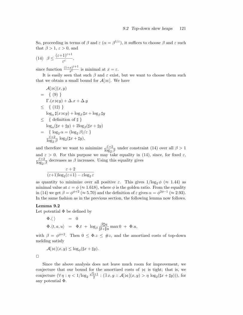
9.2 Top-down skew heaps 121
So, proceeding in terms of β and ε (α = β1/ε), it suffices to choose β and ε suchthat β > 1, ε > 0, and
β ≤ (ε+1)ε+1
εε,(14)
since function (1+x)ε+1
xε is minimal at x = ε.It is easily seen that such β and ε exist, but we want to choose them such
that we obtain a small bound for A[1 ]. We have
A[1 ](x, y)= (9)
Γ.(x1 y) + ∆.x+ ∆.y≤ (12)
logα ](x1 y) + logβ ]x+ logβ ]y
≤ definition of ] logα(]x+ ]y) + 2logβ(]x+ ]y)
= log2 α = (log2 β)/ε ε+2
log2 βlog2(]x+ ]y),
and therefore we want to minimize ε+2log2 β
under constraint (14) over all β > 1
and ε > 0. For this purpose we may take equality in (14), since, for fixed ε,ε+2
log2 βdecreases as β increases. Using this equality gives
ε+ 2(ε+1)log2(ε+1)− εlog2 ε
as quantity to minimize over all positive ε. This gives 1/log2 φ (≈ 1.44) asminimal value at ε = φ (≈ 1.618), where φ is the golden ratio. From the equalityin (14) we get β = φφ+2 (≈ 5.70) and the definition of ε gives α = φ2φ−1 (≈ 2.93).In the same fashion as in the previous section, the following lemma now follows.
Lemma 9.2Let potential Φ be defined by
Φ.〈 〉 = 0
Φ.〈t, a, u〉 = Φ.t + logββ]u]t+]u max 0 + Φ.u,
with β = φφ+2. Then 0 ≤ Φ.z ≤ #z, and the amortized costs of top-downmelding satisfy
A[1 ](x, y) ≤ logφ(]x+ ]y).
2
Since the above analysis does not leave much room for improvement, weconjecture that our bound for the amortized costs of 1 is tight; that is, weconjecture (∀ η : η < 1/log2
√5+12 : (∃x, y :: A[1 ](x, y) > η log2(]x+ ]y))), for
any potential Φ.

122 Chapter 9 Skew heaps
9.2.5 Results for priority queue operations
We have derived the following programs for the priority queue operations:
empty.= 〈 〉
isempty.z.= z = 〈 〉
single.a.= 〈a〉
min.〈t, a, u〉 .= a
union.x.y.= x1 y
delmin.〈t, a, u〉 .= t1u.
The dots in these programs together with those in the program for 1 definecost measure T . As a result, we have that the amortized costs of empty, isempty,single, and min are O(1). Furthermore, the amortized costs of union are loga-rithmic because A[union](x, y) = 1 +A[1 ](x, y), and for delmin we have:
A[delmin](〈t, a, u〉)= definition of A
T [delmin](〈t, a, u〉) + Φ.(delmin.〈t, a, u〉)− Φ.〈t, a, u〉= definitions of delmin, T , and Φ
1 +N [1 ](t, u) + Φ.(t1u)− Φ.t− ϕ.t.u− Φ.u= definition of A
1 +A[1 ](t, u)− ϕ.t.u
≤ ϕ is nonnegative 1 +A[1 ](t, u).
Hence, A[delmin](〈t, a, u〉) is O(log ]〈t, a, u〉). Note that such a conclusion canonly be drawn if ϕ is bounded from below by a constant (e.g., if ϕ is nonnegative).
Thus—hiding the particular implementation of priority queue operations—we have as results for the amortized costs (cf. Lemma 9.2):
A[empty] is O(1)A[single](a) is O(1)A[union](p, q) ≤ 1.44 log2(2 + #[[p]] + #[[q]]) comparisonsA[isempty](p) is O(1)A[min](p) is O(1)A[delmin](p) ≤ 1.44 log2(1 + #[[p]]) comparisons.
Moreover, there exists a potential function satisfying 0 ≤ Φ.p ≤ #[[p]].
9.2.6 Comparison with Sleator and Tarjan’s results
On page 54 in [30], Sleator and Tarjan describe top-down melding as follows:“we meld by merging the right paths of the two trees and then swapping the

9.3 Intermezzo on sorting 123
left and right children of every node on the merge path except the lowest”. Ourprogram for 1 is simpler because it does not have such a strange exception.
The potential function of Sleator and Tarjan for top-down melding is roughlygiven by
ϕ.t.u =
0 , ]u ≤ ]t1 , ]t < ]u
(=⌈log2
2]u]t+]u
⌉max 0).
This potential satisfies bounds (11) if we take α = 2, γ = 0, and δ = 1. Thispotential is simpler, but the corresponding bound for A[1 ] is more than twiceas large:
A[1 ](x, y) ≤ 3 log2(]x+ ]y).
Sleator and Tarjan also discussed a “lazy” version of top-down melding thatterminates as soon as one of the heaps is empty. This corresponds to the fol-lowing version for 1 , which also follows from our derivation in Section 9.2.2:
〈 〉 1 y = yx 1 〈 〉 = x
〈t, a, u〉 1 y.= 〈u1 y, a, t〉 , y 6= 〈 〉 ∧ a ≤ m.y
x 1 〈t, a, u〉 .= 〈u1x, a, t〉 , x 6= 〈 〉 ∧ a ≤ m.x,
where m is only used for nonempty trees.For this implementation of 1 one can derive that A[1 ](〈 〉, y) = 0 ≤
Γ.(〈 〉1 y) + ∆.〈 〉+ ∆.y, provided that Γ and ∆ are nonnegative. Since γ = 0,δ = 1, and 0 ≤ ϕ.t.u ≤ 1, functions Γ and ∆ are indeed nonnegative. Byinduction it now follows that (cf. (9))
A[1 ](x, y) ≤ Γ.(x1 y) + ∆.x+ ∆.y,
from which we infer that this alternative program for 1 is at least as goodthe previous one. However, for a decreasing list s we have that N [h](s) isΩ(#s log #s) for function h defined in Section 9.2.2, so the amortized cost of 1
is still logarithmic. We conjecture that 1.44 log2(]x+ ]y) is also a tight boundfor A[1 ](x, y) in this case .
9.3 Intermezzo on sorting
As illustration of the usage of skew heaps, we analyze to what extent sortingcan be done efficiently using skew heaps. One way is to use top-down skewheaps in program sort1 (see Section 9.1); then computation of sort1.s takes2.88#s log2 #s + O(#s) comparisons in the worst-case. However, with a moresophisticated implementation of function f in sort1 we obtain a sorting programthat uses at most 1.44#s log2 #s + O(#s) comparisons. The idea is to see toit that in each application of union only priority queues of about equal size areunited, so that computation of f.s takes O(#s) time only.

124 Chapter 9 Skew heaps
PQsort = g f|[f = f1 f0
|[ f0.[ ] = [ ]f0.(a` r) = f0.r a single.af1.[ ] = emptyf1.[p] = pf1.(p` q ` ps) = f1.(psa union.p.q)
]|g.p = [ ] , isempty.p
min.p` g.(delmin.p) ,¬isempty.p]|.
Remark 9.3Of course, PQsort is not intended as a practical application of mergeable priorityqueues. If it is only for the above program, it is better to take the set of ascendinglists of integers as definition for S in Section 9.2.1. Implementing union.p.q asthe merge of lists p and q and implementing the other operations in the obviousway, the above program then reduces to Mergesort (see Example 4.4), whichtakes at most #s log2 #s comparisons. (By the way, merging ascending listsmay be considered as a special case of melding heaps. This is reflected by thefollowing program for merging:
[ ] 1 [ ] = [ ](a`u) 1 y = a`u1 y , a ≤ m.y
x 1 (a`u) = a`u1x , a ≤ m.x,
where m.[ ] = ∞ and m.(a`u) = a. To compute x1 y, however, this programtakes O(#x+ #y) time instead of logarithmic time for top-down skew heaps.)2
It is not trivial that A[f ](s), which equals T [f ](s) + Φ.(f.s), is linear in #s.To show this formally, we introduce amortized costs for the components of f :
A[f0](s) = T [f0](s) + Φ∗.(f0.s)A[f1](ps) = T [f1](ps) + Φ.(f1.ps)− Φ∗.ps,
such that A[f ](s) = A[f0](s)+A[f1](f0.s). Here, potential Φ∗ is defined for listsof priority queues by Φ∗.[ ] = 0 and Φ∗.(p` ps) = Φ.p+ Φ∗.ps.
Since it is easy to show that A[f0](s) is linear in #s, we focus our attentionon A[f1], for which we have the following recurrence relation:
A[f1]([ ]) = A[empty]A[f1]([p]) = 0A[f1](p` q ` ps) = A[union](p, q) +A[f1](psa union.p.q).
In order that A[f1](s) is linear, it is important that in each application of uniononly priority queues of about equal sizes are united (more precisely, they differat most a factor of two in size). This fact is exploited in the following lemma.

9.3 Intermezzo on sorting 125
Lemma 9.4For all natural k and l,
A[f1](ps) ≤ A[empty] + 1.44 2k (Σ i : 1 ≤ i ≤ k : (l + 1 + i)/2i),
provided ps satisfies:
(i) #ps ≤ 2k
(ii) (∀ i : 0 ≤ i < #ps : #[[ps.i]] ≤ 2l).
Proof By induction on k.
Case k = 0. Then A[f1](ps) is either A[empty] or 0, hence at most A[empty].
Case k = m+1. We consider b#ps/2c successive unfoldings of f1. The resultof these unfoldings is called qs, and may be defined as follows. In case #ps iseven, list qs satisfies #qs = #ps/2, and qs.i = union.(ps.(2i)).(ps.(2i+1)) for0≤i<#qs. In case #ps is odd, #qs = (#ps+1)/2, qs.0 = ps.(#ps−1), andqs.(i+1) = union.(ps.(2i)).(ps.(2i+1)) for 0≤i<#qs−1.
Now we may apply the induction hypothesis to qs, since #qs ≤ 2m (cf. (i))and #[[qs.i]] ≤ 2l+1 (cf. (ii)):
A[f1](ps)= unfold recurrence relation for A[f1] b#ps/2c times
(Σ i : 0 ≤ i < b#ps/2c : A[union](ps.(2i), ps.(2i+1))) +A[f1](qs)≤ bound for A[union], see Section 9.2.5
(Σ i : 0 ≤ i < b#ps/2c : 1.44log2(2+#[[ps.(2i)]]+#[[ps.(2i+1]]))+A[f1](qs)≤ (ii) and l ≥ 0; b#ps/2c ≤ 2m
1.44 2m(l+2) +A[f1](qs)≤ induction hypothesis
1.44 2m(l+2) +A[empty] + 1.44 2m (Σ i : 1 ≤ i ≤ m : (l+2+i)/2i)= calculus
A[empty] + 1.44 2m+1 (Σ i : 0 ≤ i ≤ m : (l+1+i+1)/2i+1)= k = m+1
A[empty] + 1.44 2k (Σ i : 1 ≤ i ≤ k : (l+1+i)/2i).
2
Instantiation of this lemma with k = dlog2(#s+1)e, l = 0, and ps = f0.s yields,using #(f0.s) = #s:
A[f1](f0.s) ≤ A[empty] + 2.88(#s+1) (Σ i : 1 ≤ i ≤ dlog2(#s+1)e :i+12i
).
This implies that A[f1](f0.s) is O(#s), since the summation has the same orderof magnitude as
∫∞0
x+12x dx, which is O(1). Hence, we have shown that A[f ](s)
is linear in s (and also that T [f ](s) is linear).

126 Chapter 9 Skew heaps
9.4 Bottom-up skew heaps
Reconsidering the derivation of the top-down skew heaps we conclude that thedecision to use binary trees as representations for bags is in fact the main designdecision. Keeping matters as simple as possible, the introduction of the heapcondition and the operator 1 followed in a natural way. The implementationsderived for 1 both have logarithmic amortized costs and there seems to be noway to improve this. In [30], however, Sleator and Tarjan present the bottom-up skew heaps as alternative implementation of priority queues. For bottom-upskew heaps they achieve a logarithmic bound for the amortized costs of delminand O(1) bounds for the remaining operations; hence, the amortized costs ofunion are reduced to O(1). How come?
Well, Sleator and Tarjan still use binary trees to represent bags, but—formally speaking—they take a different view of binary trees. In the previoussection we have introduced set 〈Int〉 in the common way, viz. as the smallestsolution of
X : X = 〈 〉 ∪ X×Int×X.
This “top-down” view of binary trees forces us to dissect a nonempty tree intoits left subtree, its root, and its right subtree, and in this way we are almostinescapably led to the programs found for 1 . It appears that the way oneintroduces binary trees constitutes an important design decision, for we have totake a special view of binary trees to arrive at the bottom-up skew heaps.
In case of bottom-up skew heaps the following definition is appropriate. Wedefine set 〈Int〉1 as the smallest solution of
X : X = [X × Int].
We have already described this tree type in Section 6.2.2, from which we recallthat elements of 〈Int〉1 are interpreted as binary trees in the following way: [ ]stands for the empty tree and 〈t, a〉 `u for a nonempty tree with left subtree t,root a, and right subtree u. In addition, we will use that nonempty elements of〈Int〉1 can be dissected as ua 〈t, a〉 (where a is the last element of the inordertraversal of this tree). For the programs in the sequel the following algebra isappropriate:
( 〈Int〉1 | [ ], (=[ ]), [·], ++ , hd, tl, lt, ft ).
As shown in Section 6.2.2, there exists a destructive implementation for thisalgebra that supports all operations in O(1) time.
Since there is a clear correspondence between 〈Int〉 and 〈Int〉1, we omit thedefinitions of functions like [[·]], m, and H for the latter type. However, doingthe same for # would make #z ambiguous (for z ∈ 〈Int〉1). We resolve thisambiguity by interpreting #z as the length of list z. To denote the size of thetree associated with z we write #[[z]].
To obtain a definition of SH, we simply write the definitions for top-downskew heaps in terms of type 〈Int〉1. This gives for S:
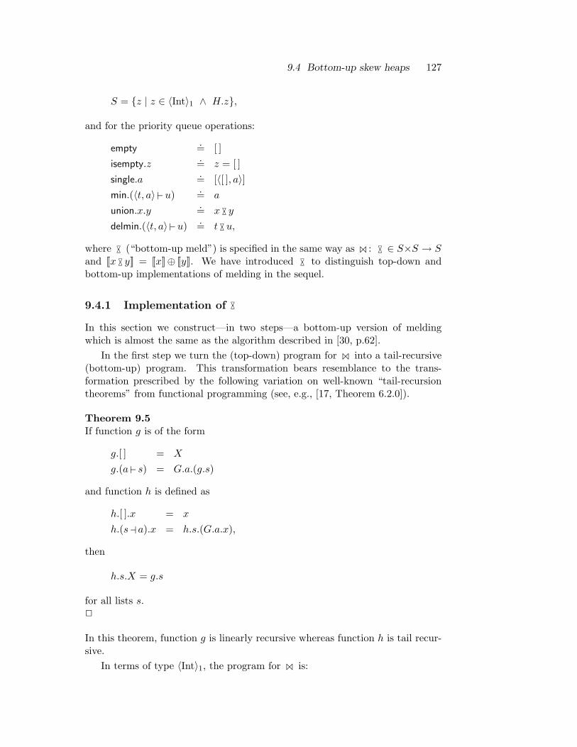
9.4 Bottom-up skew heaps 127
S = z | z ∈ 〈Int〉1 ∧ H.z,
and for the priority queue operations:
empty.= [ ]
isempty.z.= z = [ ]
single.a.= [〈[ ], a〉]
min.(〈t, a〉 `u) .= a
union.x.y.= x MO y
delmin.(〈t, a〉 `u) .= t MOu,
where MO (“bottom-up meld”) is specified in the same way as 1 : MO ∈ S×S → Sand [[x MO y]] = [[x]]⊕ [[y]]. We have introduced MO to distinguish top-down andbottom-up implementations of melding in the sequel.
9.4.1 Implementation of MO
In this section we construct—in two steps—a bottom-up version of meldingwhich is almost the same as the algorithm described in [30, p.62].
In the first step we turn the (top-down) program for 1 into a tail-recursive(bottom-up) program. This transformation bears resemblance to the trans-formation prescribed by the following variation on well-known “tail-recursiontheorems” from functional programming (see, e.g., [17, Theorem 6.2.0]).
Theorem 9.5If function g is of the form
g.[ ] = X
g.(a` s) = G.a.(g.s)
and function h is defined as
h.[ ].x = x
h.(sa a).x = h.s.(G.a.x),
then
h.s.X = g.s
for all lists s.2
In this theorem, function g is linearly recursive whereas function h is tail recur-sive.
In terms of type 〈Int〉1, the program for 1 is:

128 Chapter 9 Skew heaps
[ ] 1 [ ] = [ ](〈t, a〉 `u) 1 y
.= 〈u1 y, a〉 ` t , a ≤ m.yx 1 (〈t, a〉 `u) .= 〈u1x, a〉 ` t , a ≤ m.x.
As in Theorem 9.5, we introduce a function F , say, with one more parameterthan 1 , and we use a recursion pattern based on a instead of ` to define F .Then x1 y = F.x.y.[ ] (see after Lemma 9.6), where
F.[ ].[ ].z = z
F.(ua 〈t, a〉).y.z .= F.u.y.(〈z, a〉 ` t) , a ≥M.y
F.x.(ua 〈t, a〉).z .= F.u.x.(〈z, a〉 ` t) , a ≥M.x,
with M defined by
M.[ ] = −∞M.(ua 〈t, a〉) = a.
(Note that, in general, M.z differs from the maximum of [[z]], for heap z.) Therelation between F and 1 is expressed in Lemma 9.6, in which we use thefollowing characterization of H for 〈Int〉1-trees:
H.[ ] ≡ trueH.(ua 〈t, a〉) ≡ H.u ∧ M.u ≤ a ∧ a ≤ m.t ∧ H.t.
(15)
Lemma 9.6For all heaps x, y, v, and w satisfying M.xmaxM.y ≤ m.vminm.w:
F.x.y.(v1w) = (x++ v) 1 (y++w).
Proof Note that the premiss implies that x++ v and y++w are heaps. Theproof proceeds by induction on x and y, using the following exhaustive caseanalysis.
Case x = [ ] ∧ y = [ ]. By the definition of F , F.[ ].[ ].(v1w) = v1w.
Case x = ua 〈t, a〉 ∧ a ≥M.y. Then M.xmaxM.y = a, and for all heaps vand w satisfying a ≤ m.v ∧ a ≤ m.w we have:
F.(ua 〈t, a〉).y.(v1w)= definition of F (a ≥M.y) F.u.y.(〈v1w, a〉 ` t)
= definition of 1 (a ≤ m.w) F.u.y.((〈t, a〉 ` v) 1w)
= induction hypothesis (M.umaxM.y ≤ aminm.w, see below) (u++(〈t, a〉 ` v))1 (y++w)
= list calculus ((ua 〈t, a〉) ++ v) 1 (y++w).

9.4 Bottom-up skew heaps 129
Since x is a heap, we have H.u ∧ M.u ≤ a ∧ a ≤ m.t ∧ H.t (cf. (15)). Inconjunction with a ≤ m.v ∧ H.v, this implies H.(〈t, a〉 ` v).Case y = ua 〈t, a〉 ∧ a ≥M.x. This case follows by symmetry.2
Instantiation of this lemma with v = [ ] and w = [ ] gives F.x.y.[ ] = x1 y.Furthermore, we have N [F ](x, y, [ ]) = N [1 ](x, y), where N denotes the costmeasure for the above programs. So, the introduction of F does not give animprovement. However, we are now ready for our second step in which weextend the base case for F.x.y.z from x = [ ] ∧ y = [ ] to x = [ ] ∨ y = [ ]. As aresult, we will obtain a program for MO with O(1) amortized costs, whereas thesame extension applied to the program for 1 gives no essential reduction (seeSection 9.2.6).
We observe that M.xmaxM.y ≤ m.z holds as precondition for all (recursive)applications F.x.y.z generated during the evaluation of F.x.y.[ ]. For x = [ ], thisis equivalent to M.y ≤ m.z, and consequently, y++ z is a heap. Since we assumethat ++ takes O(1) time for 〈Int〉1-trees, we simply take this for F.[ ].y.z. Bysymmetry, we take F.x.[ ].z = x++ z, and we obtain as program for MO :
x MO y = F.x.y.[ ]
|[ F.[ ].y.z = y++ z
F.(ua 〈t, a〉).y.z .= F.u.y.(〈z, a〉 ` t) , a ≥M.y ∧ y 6= [ ]F.x.[ ].z = x++ z
F.x.(ua 〈t, a〉).z .= F.u.x.(〈z, a〉 ` t) , a ≥M.x ∧ x 6= [ ]]|.
In this program, M is used for nonempty trees only.Compared to the program for 1 , the program for MO is more intricate and
so will be its analysis. In a first, exploratory analysis we will strive for an O(1)bound for the amortized costs of MO . Unfortunately, this results in a linear boundfor delmin, which is not what we are after. In Section 9.4.3 we will thereforecombine the result of the next section with our approach to top-down skew heapsso as to obtain a logarithmic bound for delmin.
9.4.2 Bottom-up analysis of MO
As before, we use N to denote the cost measure defined by the dots in theabove program. This measure exactly counts the number of comparisons. Theamortized costs for MO are defined as usual.
A[ MO ](x, y) = N [ MO ](x, y) + Φ.(x MO y)− Φ.x− Φ.y.
However, the pattern of the definition of the amortized costs for F , given by
A[F ](x, y, z) = N [F ](x, y, z) + Φ.(F.x.y.z)− Φ.x− Φ.y,

130 Chapter 9 Skew heaps
deviates from the general pattern used thus far. We have omitted “−Φ.z”, forotherwise it is impossible—as far as we know—to define Φ such that A[F ] isO(1). As a possible explanation, we remark that we use F in such a way thatz is merely an accumulation parameter, whereas x and y are input parametersand F.x.y.z is the result.
From the program for MO , it is immediate that A[ MO ](x, y) = A[F ](x, y, [ ]).Our goal is now to define Φ such that A[F ] is O(1). To achieve this, we changethe above program for F a little bit because an analysis of this program alongthe same lines as below leads to a potential function for which A[F ] is not O(1).We shall therefore study the following equivalent program for F , which we haveobtained by singling out the cases in which one of the first two arguments is asingleton list:
F.[ ].y.[ ] = y
F.[〈t, a〉].y.z .= y++(〈z, a〉 ` t) , a ≥M.y ∧ y 6= [ ]F.(ua 〈t, a〉).y.z .= F.u.y.(〈z, a〉 ` t) , a ≥M.y ∧ y 6= [ ] ∧ u 6= [ ].
The symmetric counterparts of these alternatives are omitted.We first consider the recursive case for F , since this puts the strongest re-
quirements on Φ (u 6= [ ]):
A[F ](ua 〈t, a〉, y, z)= definition of A
N [F ](ua 〈t, a〉, y, z) + Φ.(F.(ua 〈t, a〉).y.z)− Φ.(ua 〈t, a〉)− Φ.y= definitions of F and N
1 +N [F ](u, y, 〈z, a〉 ` t) + Φ.(F.u.y.(〈z, a〉 ` t))− Φ.(ua 〈t, a〉)− Φ.y= definition of A
A[F ](u, y, 〈z, a〉 ` t) + 1 + Φ.u− Φ.(ua 〈t, a〉).
In order to obtain an O(1) bound for A[F ] we define Φ such that 1 + Φ.u −Φ.(ua 〈t, a〉) ≤ 0. To keep Φ as small as possible, we even take
Φ.(ua 〈t, a〉) = Φ.u+ 1,(16)
for u 6= [ ].Taking Φ.[ ] = 0 gives A[F ]([ ], y, [ ]) = 0, and for the remaining nonrecursive
case we derive (y 6= [ ]):
A[F ]([〈t, a〉], y, z)= definition of A
N [F ]([〈t, a〉], y, z) + Φ.(F.[〈t, a〉].y.z)− Φ.[〈t, a〉]− Φ.y= definition of F and N
1 + Φ.(y++(〈z, a〉 ` t))− Φ.[〈t, a〉]− Φ.y= (16) implies Φ.(y++(〈z, a〉 ` t)) = Φ.y + 1 + #t, for y 6= [ ]

9.4 Bottom-up skew heaps 131
1 + 1 + #t− Φ.[〈t, a〉]= take Φ.[〈t, a〉] = #t+ 1 (see definition Φ below)
1.
Hence, A[F ](x, y, z) ≤ 1, if we define Φ as follows:
Φ.[ ] = 0Φ.(〈t, a〉 `u) = #t+ 1 + #u,
and, consequently, A[ MO ](x, y) ≤ 1. (We leave it to the reader to ascertain thata similar analysis of the program derived in Section 9.4.1 leads to potentialΦ.z = #z, for which A[F ] is not O(1).)
Remark 9.7The above derived potential Φ is reminiscent of the potential used by Sleatorand Tarjan in their analysis of bottom-up skew heaps. In their terminology,Φ.x equals the sum of the lengths of the major path and the minor path of x.(The major path of x is the rightmost path of x, and the minor path of x is therightmost path of x’s left subtree)2
With T as defined for top-down skew heaps, we now have O(1) bounds forall priority queue operations, except that for delmin:
A[delmin](〈t, a〉 `u)= definition of A
T [delmin](〈t, a〉 `u) + Φ.(delmin.(〈t, a〉 `u))− Φ.(〈t, a〉 `u)= definitions of delmin and Φ
1 +N [ MO ](t, u) + Φ.(t MOu)−#t− 1−#u= definition of A
A[ MO ](t, u) + Φ.t−#t+ Φ.u−#u≤ bound for A[ MO ]
1 + Φ.t−#t+ Φ.u−#u.
Unfortunately, Φ.z − #z may be linear in the size of z, and therefore we canonly conclude that A[delmin](z) is linear in the size of z.
9.4.3 First top-down analysis of MO
To obtain a logarithmic bound for the amortized costs of delmin we analyzeyet another (equivalent) program for MO . Inspired by the potential function ofSleator and Tarjan for bottom-up skew heaps, we take a potential function ofthe following form:
Φ.〈 〉 = 0Φ.〈t, a, u〉 = Ψ.〈t, a, u〉+ Π.t+ Π.〈t, a, u〉,

132 Chapter 9 Skew heaps
with
Ψ.〈 〉 = 0Ψ.〈t, a, u〉 = Ψ.t+ ψ.t.u+ Ψ.u,
and
Π.〈 〉 = 0Π.〈t, a, u〉 = π.t.u+ Π.u.
The form of Φ may be considered as a mixture of the form of the potentialfunction for top-down skew heaps (Ψ) and the form of the potential functionfound in the previous section (Π, twice).
Remark 9.8 (see Remark 9.7)In the above form for Φ, the nodes on the major path and those on the minor pathare treated as special—as is also done in [30]. The term Π.〈t, a, u〉 correspondsto the major path and Π.t to the minor path.2
Our analysis of top-down skew heaps proceeded smoothly because the re-cursion pattern in the program of 1 matched the recursive definition of thepotential so well. In view of the above definition of Φ we therefore decide toconstruct a top-down simulation (read “algorithmic refinement”) of MO . Thissimulation is based on the observation that x MO y = t++(u1 y) if m.x ≤ m.y,where t and u satisfy t++u = x and M.t ≤ m.y ≤ m.u. Phrased differently,x MO y can be computed in two stages: first compute t and then compute u1 y.This is encoded in the following program:
〈 〉 MO 〈 〉 = 〈 〉〈t, a, u〉 MO y = 〈t, a, u / y〉 , a ≤ m.y
x MO 〈t, a, u〉 = 〈t, a, u / x〉 , a ≤ m.x,
where
〈 〉 / 〈 〉 = 〈 〉〈t, a, u〉 / y = 〈t, a, u / y〉 , a ≤ m.y
x / 〈t, a, u〉 .= 〈u1x, a, t〉 , a ≤ m.x,
and where
〈 〉 1 〈 〉 = 〈 〉〈t, a, u〉 1 y
.= 〈u1 y, a, t〉 , a ≤ m.yx 1 〈t, a, u〉 .= 〈u1x, a, t〉 , a ≤ m.x.
Note that some of the above definitions are longer than necessary (e.g., thedefinition of MO ). The uniformity of the above definitions, however, turns out tobe the basis for a smooth amortized analysis. The cost measure N for the above

9.4 Bottom-up skew heaps 133
program has been chosen such that it coincides with the cost measure for thebottom-up program for MO .
To facilitate the calculations below, we introduce functions Θ and θ, definedby Θ.z = Ψ.z + Π.z and θ.t.u = ψ.t.u+ π.t.u. Then
Θ.〈 〉 = 0Θ.〈t, a, u〉 = Ψ.t+ θ.t.u+ Θ.u,
and
Φ.〈 〉 = 0Φ.〈t, a, u〉 = Θ.t+ θ.t.u+ Θ.u,
as a consequence of which Π and π become superfluous. Recall that the amor-tized costs of MO are defined as
A[ MO ](x, y) = N [ MO ](x, y) + Φ.(x MO y)− Φ.x− Φ.y.
In what follows, we will derive suitable definitions for A[/ ] and A[1 ].
Six requirements on θ and ψ
In order that Φ is nonnegative and small, we require that θ and ψ satisfy
(i) 0 ≤ θ.t.u
(ii) 0 ≤ ψ.t.u,
and also that θ and ψ are small. In the sequel we will accumulate further require-ments on θ and ψ that ensure that A[ MO ] is O(1) and A[delmin] is logarithmic.
For A[ MO ] we have A[ MO ](〈 〉, 〈 〉) = 0, and in case x MO y = 〈t, a, u / y〉, wederive:
A[ MO ](x, y)= definition of A[ MO ]
N [ MO ](x, y) + Φ.(x MO y)− Φ.x− Φ.y= definitions of N and Φ (x = 〈t, a, u〉)
N [/ ](u, y) + Θ.t+ θ.t.(u / y) + Θ.(u / y)−Θ.t− θ.t.u−Θ.u− Φ.y= definition of A[/ ] (see below)
A[/ ](u, y) + θ.t.(u / y)− θ.t.u.
The appropriate definition for the amortized cost of / is thus given by
A[/ ](x, y) = N [/ ](x, y) + Θ.(x / y)−Θ.x− Φ.y.
Simply turning the handle gives A[/ ](〈 〉, 〈 〉) = 0, and for the case x / y =〈t, a, u / y〉:

134 Chapter 9 Skew heaps
A[/ ](x, y) = A[/ ](u, y) + θ.t.(u / y)− θ.t.u.
In case x / y = 〈u1x, a, t〉, we derive the definition of A[1 ] as follows:
A[/ ](x, y)= definition of A[/ ]
N [/ ](x, y) + Θ.(x / y)−Θ.x− Φ.y= definitions of N and Θ (y = 〈t, a, u〉)
1 +N [1 ](u, x) + Ψ.(u1x) + θ.(u1x).t+ Θ.t−Θ.x−Θ.t− θ.t.u−Θ.u= definition of A[1 ] (see below)
A[1 ](u, x) + 1 + θ.(u1x).t− θ.t.u,
where the amortized cost of 1 is defined by
A[1 ](x, y) = N [1 ](x, y) + Ψ.(x1 y)−Θ.x−Θ.y.
Omitting the calculations for A[1 ], we thus obtain as recurrence relations:
A[ MO ](〈 〉, 〈 〉) = 0
A[ MO ](〈t, a, u〉, y) = A[/ ](u, y) + θ.t.(u / y)− θ.t.u , a ≤ m.y
A[ MO ](x, 〈t, a, u〉) = A[/ ](u, x) + θ.t.(u / x)− θ.t.u , a ≤ m.x
A[/ ](〈 〉, 〈 〉) = 0
A[/ ](〈t, a, u〉, y) = A[/ ](u, y) + θ.t.(u / y)− θ.t.u , a ≤ m.y
A[/ ](x, 〈t, a, u〉) = A[1 ](u, x) + 1 + θ.(u1x).t− θ.t.u , a ≤ m.x
A[1 ](〈 〉, 〈 〉) = 0
A[1 ](〈t, a, u〉, y) = A[1 ](u, y) + 1 + ψ.(u1 y).t− θ.t.u , a ≤ m.y
A[1 ](x, 〈t, a, u〉) = A[1 ](u, x) + 1 + ψ.(u1x).t− θ.t.u , a ≤ m.x.
Solving A[ MO ] from this set of recurrence relations leads to at most one un-folding of the last alternative of A[/ ]. In order that A[ MO ] is O(1), it is thereforesufficient to require that the term 1 + θ.(u1x).t − θ.t.u is bounded, while theother terms are required to be nonpositive. Thus, we require that, for someconstant γ and for all t, u, x and y:
(iii) θ.t.(u / y) ≤ θ.t.u
(iv) θ.(u1x).t ≤ θ.t.u+ γ
(v) 1 + ψ.(u1 y).t ≤ θ.t.u.
If we succeed in fulfilling these five requirements, we may conclude from theabove set of recurrence relations that A[ MO ](x, y) ≤ γ + 1. These requirementsare, of course, easily met when we choose ψ.t.u = 0 and θ.t.u = 1; then Φcoincides with the potential function derived in Section 9.4.2. There is, however,an additional requirement to ensure a logarithmic bound for delmin:

9.4 Bottom-up skew heaps 135
A[delmin](〈t, a, u〉)= definition of A
T [delmin](〈t, a, u〉) + Φ.(delmin.〈t, a, u〉)− Φ.〈t, a, u〉= definitions of T ,delmin, and Φ
1 +N [ MO ](t, u) + Φ.(t MOu)−Θ.t− θ.t.u−Θ.u= definition of A
1 +A[ MO ](t, u) + Φ.t+ Φ.u−Θ.t− θ.t.u−Θ.u≤ above bound for A[ MO ]; θ nonnegative (requirement (i)) γ + 2 + Φ.t−Θ.t+ Φ.u−Θ.u
≤ Φ.z −Θ.z ≤ logα ]z, see below γ + 2 + logα ]t+ logα ]u
≤ 4mn ≤ (m+ n)2 γ + 2 + 2 logα(]t+ ]u)− logα 4.
We choose ψ and θ such that Φ.z −Θ.z ≤ logα ]z, for some constant α, α > 1.Evidently, this is true for z = 〈 〉. For z = 〈t, a, u〉, we have that Φ.z−Θ.z = Π.t,and therefore we want Π to satisfy
Π.z ≤ logα ]z,(17)
for all z. To obtain a requirement in terms of ψ and θ, we first translate thisrequirement on Π into a requirement on π. We apply induction on z.
Case z = 〈 〉. Trivial, since ]〈 〉 = 1.
Case z = 〈t, a, u〉.
Π.〈t, a, u〉= definition of Π π.t.u+ Π.u
= induction hypothesis (17) π.t.u+ logα ]u
≤ see upper bound for π below logα ]〈t, a, u〉.
Hence, we require that π.t.u is bounded from above by logα]t+]u]u , or, in terms
of θ and ψ:
(vi) θ.t.u− ψ.t.u ≤ logα]t+]u]u .
This concludes the derivation of six requirements on ψ and θ, which are sufficientto ensure that the amortized cost of delmin is logarithmic and that the amortizedcosts of the other priority queue operations are O(1). In addition, we obtain anonnegative and small potential Φ, provided ψ and θ are small.

136 Chapter 9 Skew heaps
Construction of θ and ψ
First of all, we remark that (i) is redundant, since it follows from (ii) and (v).Next, we do away with logα in requirement (vi) by introducing functions f andg and defining
θ.t.u = logα f.]t.]u
ψ.t.u = logα g.]t.]u.
Apart from the removal of logα, the introduction of f and g embodies the decisionto let θ.t.u and ψ.t.u depend on the sizes of t and u only—this simplifies theformulation of the requirements and for top-down skew heaps we also found thatϕ.t.u depends on the sizes of t and u only. The corresponding requirements onf and g then read ((i) is redundant; constant β replaces αγ):
(i) 1 ≤ f.k.l
(ii) 1 ≤ g.k.l
(iii) f.k.m ≤ f.k.l
(iv) f.m.k ≤ β f.k.l
(v) α g.m.k ≤ f.k.l
(vi) f.k.lg.k.l ≤
k + ll ,
for all positive k, l, and m such that l ≤ m (α > 1 and β > 0).In our next step, we get rid of m in requirements (iv) and (v). Firstly, we
may replace (iv) by (iv′), with
(iv′) f.l.k ≤ β f.k.l ,
because (iv′) is not weaker than (iv) on account of (iii):
f.m.k
≤ (iv′) β f.k.m
≤ (iii) β f.k.l,
for any k, l, and m with l ≤ m. On similar grounds, (v) may be replaced by(v′), where
(v′) α g.l.k ≤ f.k.l.
Now we observe that it is necessary that α ≤ β, since it is required that forall k and l:

9.4 Bottom-up skew heaps 137
α
≤ (v′) f.k.lg.l.k
≤ (iv′)
β f.l.kg.l.k
≤ (vi)
β l + kk .
Since we want α to be as large as possible and β as small as possible, we takeα = β.
As a further simplification we decide to eliminate g from the set of require-ments. To this end we define
g.k.l =f.l.k
α,
i.e., we choose equality in (v′). This choice for g does not strengthen the re-
quirements on f and α: requirement (vi) becomes α f.k.lf.l.k ≤ k + l
l , but this
already follows from (v′) and (vi). Taking k = l in (vi) then gives α ≤ 2, sowe take α = 2 (as large as possible). As a result, we obtain the following set ofrequirements for f , where we have swapped k and l in (III) to let it resemble(IV):
(I) 2 ≤ f.k.l ≤ 4(II) f.k.m ≤ f.k.l
(III) f.k.l ≤ 2 f.l.k
(IV) f.k.l ≤ k + l2l f.l.k,
for all positive k, l, and m such that l ≤ m. In (I) we have added an absoluteupper bound for f to make explicit how small we want f to be; we have chosen4 because (∀ k, l :: 2 ≤ f.k.l ≤ δ) implies (∀ k, l :: 4l ≤ δ(k + l)) on account of(IV), hence it is necessary that δ ≥ 4.
Requirements (I) through (III) are satisfied if we take f.k.l = 2, but then(IV) does not hold if k < 3l. To arrive at a solution for f , we distinguish thecases k ≤ l and k ≥ l in the definition of f.k.l. By simply taking f.k.l = 2 in casek ≤ l, we see that (IV) reduces to 2 ≤ k + l
2l f.l.k. To satisfy this requirementwe define f such that we have equality in (IV). The resulting f is then given by
f.k.l = 2k + kmax l
k + l.
The reader may now verify that this definition meets all requirements on f .

138 Chapter 9 Skew heaps
Remark 9.9By first taking f.k.l = 2 in case k ≥ l and subsequently taking equality in (IV)as above, we find:
f.k.l = 4k + l
kmax l + l.
The choice for f in the text is preferred because it results in a smaller potential.2
Thus we find (since g.k.l = f.l.k/2):
ψ.t.u = log2]tmax ]u + ]u
]t + ]u (= log22]u]t+]u max 0),
and θ.t.u = 1 + ψ.u.t. Since 0 ≤ ψ.t.u ≤ 1, potential Φ satisfies 0 ≤ Φ.z ≤ 2#z.With this potential, each priority queue operation except delmin has O(1)
amortized costs. The amortized costs of the latter operation satisfy
A[delmin](〈t, a, u〉)≤ see page 135 γ + 2 + 2 logα(]t+ ]u)− logα 4
= α = 2, β = 2, and γ = logα β = 1 1 + 2 log2 ]〈t, a, u〉,
which completes the proof of the following lemma.
Lemma 9.10Let potential Φ be defined by
Φ.〈 〉 = 0
Φ.〈t, a, u〉 = Θ.t + log24]t]t+]u max 1 + Θ.u
with
Θ.〈 〉 = 0
Θ.〈t, a, u〉 = Ψ.t + log24]t]t+]u max 1 + Θ.u
Ψ.〈 〉 = 0
Ψ.〈t, a, u〉 = Ψ.t + log22]u]t+]u max 0 + Ψ.u.
Then 0 ≤ Φ.z ≤ 2#z, and the amortized costs of union and delmin satisfy
A[union](x, y) ≤ 3A[delmin](z) ≤ 1 + 2 log2 ]z.
2

9.4 Bottom-up skew heaps 139
Remark 9.11 (see Remark 9.7)In Sleator and Tarjan’s analysis of bottom-up skew heaps, a node with subtreest and u contributes dψ.t.ue + 2dψ.u.te if it is on the major or minor path, anddψ.t.ue otherwise. Since dψ.t.ue + 2dψ.u.te ≈ 1 + ψ.u.t, this may be comparedto our potential that counts 1 + ψ.u.t for nodes on the major and minor pathsand ψ.t.u for the remaining nodes.2
9.4.4 Second top-down analysis of MO
Although the O(1) bound for union is a nice result, it is somewhat disappointingthat the bound for delmin.p is as high as 2 log2(#[[p]] + 1). These bounds implythat at most 2N log2N comparisons are needed to sort N numbers by means ofbottom-up skew heaps (since this requires N applications of delmin). As shownin Section 9.3, however, we have 1.44N log2N as bound when top-down skewheaps are used, and we would like to have a similar bound for bottom-up skewheaps.
To achieve this, we allow logarithmic costs for MO . For α > 1, we try asbound:
A[ MO ](x, y) ≤ 1 + logα(]x+ ]y).(18)
To take advantage of the work done to analyze top-down skew heaps, we take
θ.t.u = 1,
and we derive several requirements for the remaining function ψ. This choicefor θ considerably simplifies the recurrence relations for the amortized costs inthe analysis of MO in the previous section:
A[ MO ](〈 〉, 〈 〉) = 0A[ MO ](〈t, a, u〉, y) = A[/ ](u, y) , a ≤ m.y
A[ MO ](x, 〈t, a, u〉) = A[/ ](u, x) , a ≤ m.x
A[/ ](〈 〉, 〈 〉) = 0A[/ ](〈t, a, u〉, y) = A[/ ](u, y) , a ≤ m.y
A[/ ](x, 〈t, a, u〉) = A[1 ](u, x) + 1 , a ≤ m.x
A[1 ](〈 〉, 〈 〉) = 0A[1 ](〈t, a, u〉, y) = A[1 ](u, y) + ψ.(u1 y).t , a ≤ m.y
A[1 ](x, 〈t, a, u〉) = A[1 ](u, x) + ψ.(u1x).t , a ≤ m.x.
To solve (18), we first observe—as in our analysis of top-down skew heaps (cf.(9))—that

140 Chapter 9 Skew heaps
A[1 ](x, y) = Γ.(x1 y),
where
Γ.〈 〉 = 0Γ.〈t, a, u〉 = Γ.t+ ψ.t.u.
Since A[ MO ](x, y) ≤ 1 +A[1 ](x, y), we see that (18) is satisfied when
Γ.z ≤ logα ]z,
which is in turn satisfied when
(i) ψ.t.u ≤ logα]t+]u]t .
To obtain logarithmic amortized costs for delmin, we want in addition—cf.(17)—that
Π.z ≤ logβ ]z,(19)
for some β > 1, which leads to the following requirement on ψ:
(ii) 1− ψ.t.u ≤ logβ]t+]u]u .
As shown in Section 9.2.4, the existence of a function ψ satisfying (i) and (ii)(cf. (13)) is guaranteed provided (cf. (14))
β ≤ (ε+ 1)ε+1
εε,
where ε = logα β. Moreover, we have shown that it is possible to define ψ suchthat 0 ≤ ψ.t.u ≤ 1. Since θ.t.u = 1, we thus obtain a potential Φ satisfying0 ≤ Φ.z ≤ #z.
To obtain a small bound for delmin, we derive
A[delmin](〈t, a, u〉)= see page 135
1 +A[ MO ](t, u) + Φ.t+ Φ.u−Θ.t− θ.t.u−Θ.u= θ.t.u = 1
A[ MO ](t, u) + Φ.t−Θ.t+ Φ.u−Θ.u≤ (18); (19), using that Φ.z −Θ.z = Π.(l.z) for nonempty z
1 + logα(]t+ ]u) + logβ ]t+ logβ ]u
≤ logα x = ε logβ x 1 + (ε+ 2) logβ(]t+ ]u).
This proves the following lemma.

9.4 Bottom-up skew heaps 141
Lemma 9.12Let ε > 0 and let potential Φ be defined by
Φ.〈 〉 = 0Φ.〈t, a, u〉 = Θ.t+ 1 + Θ.u
with
Θ.〈 〉 = 0Θ.〈t, a, u〉 = Ψ.t+ 1 + Θ.uΨ.〈 〉 = 0
Ψ.〈t, a, u〉 = Ψ.t + logββ]u]t+]u max 0 + Ψ.u.
Then 0 ≤ Φ.z ≤ #z, and the amortized costs of union and delmin satisfy
A[union](x, y) ≤ logα(]x+ ]y) + O(1)A[delmin](z) ≤ (ε+ 2) logβ ]z + O(1),
where α = β1/ε and β = (ε+1)ε+1
εε .2
For each ratio of the number of union’s to the number of delmin’s, a suitablechoice for ε in Lemma 9.12 can be made. For example, if this ratio is 1, weminimize 2ε+2
log2 βover all ε > 0. This yields 2 as minimal value at ε = 1. In
this way, we get 2N log2N as bound on the number of comparisons needed byprogram sort1 to sort N numbers. Note that this bound for sort1 also followsfrom Lemma 9.10.
To obtain a good bound for PQsort, we minimize the bound for delmin. Asshown in Section 9.2.4, minimizing ε+2
log2 βyields
A[delmin](z) ≤ logφ ]z + O(1)
for ε = φ (≈ 1.618) and β = φφ+2 (≈ 5.70). The corresponding bound for unionis
A[union](x, y) ≤ logα(]x+ ]y) + O(1),
with α = φ2φ−1 (≈ 2.93). Compared to the bounds for top-down skew heaps, thisbound for union is lower whereas the bounds for delmin are equal. So, accordingto these bounds, bottom-up skew heaps are at least as good as top-down skewheaps.

142 Chapter 9 Skew heaps
9.4.5 Results for priority queue operations
With T as defined for top-down skew heaps, we have derived in Section 9.4.3the following bounds for bottom-up skew heaps (cf. Lemma 9.10):
A[empty] is O(1)A[single](a) = 1 comparisonA[union](p, q) ≤ 2 comparisonsA[isempty](p) is O(1)A[min](p) is O(1)A[delmin](p) ≤ 2 log2(1 + #[[p]]) comparisons,
for a potential function satisfying 0 ≤ Φ.p ≤ 2#[[p]]. These bounds for union anddelmin improve the bounds obtained by Sleator and Tarjan by a factor 2.
The analysis in Section 9.4.4 yields as bounds (instantiate Lemma 9.12 withε = φ):
A[empty] is O(1)A[single](a) = 1 comparisonA[union](p, q) ≤ 0.64 log2(2 + #[[p]] + #[[q]]) comparisonsA[isempty](p) is O(1)A[min](p) is O(1)A[delmin](p) ≤ 1.44 log2(1 + #[[p]]) comparisons,
for a potential function satisfying 0 ≤ Φ.p ≤ #[[p]]. These bounds for union anddelmin cannot be compared with the bounds obtained by Sleator and Tarjan,since the bound for union is not O(1) but the bound for delmin is better.
9.5 Pointer implementations
Top-down skew heaps
In the implementation of top-down skew heaps we have used algebra
( 〈Int〉 | 〈 〉, (=〈 〉), 〈·, ·, ·〉, l,m, r ).
A purely-functional implementation of this algebra, which supports all opera-tions in O(1) time, is described in Section 4.3. The only disadvantage of thisimplementation is that the recycling of cells is not trivial. This can be madetrivial by disposing cells explicitly, like we did in the destructive implementationof stacks in Chapter 4. This yields a destructive implementation of top-downskew heaps.
A next step is to recycle cells in-line to obtain an in-situ version of top-down skew heaps. That is, we avoid a call to new by using the cell which is

9.5 Pointer implementations 143
disposed by a nearby call to dispose; e.g., for the destructive implementation ofstacks, cons.a.(tl.p) is equivalent to p∧.a := a; return(p). This gives the followingdestructive implementation of top-down skew heaps at pointer level:
empty = nilisempty.p = p = nilsingle.a = |[ h:B; new(h); h∧ := 〈nil, a,nil〉; return(h) ]|min.p = p∧.a
union.p.q = p1 q
delmin.p = return(p∧.l1 p∧.r); dispose(p),
where
p1 q = q , p = nilp , q = nil( return(p); p∧.l, p∧.r := p∧.r1 q, p∧.l , p∧.a ≤ q∧.a
return(q); q∧.l, q∧.r := q∧.r1 p, q∧.l , q∧.a ≤ p∧.a
) , p 6= nil∧ q 6= nil.
Strictly speaking, the program for 1 is not in-situ yet because it is recursive. Itis however a simple form of recursion, and therefore it is not difficult to transformit into an iterative program. We leave this to the interested reader (see [30] formore details).
Bottom-up skew heaps
The algebra used in the programs for bottom-up skew heaps on pages 127and 129 is algebra T1 from Section 6.2.2:
T1 = ( 〈Int〉1 | [ ], (=[ ]), [·], ++ , hd, tl, lt, ft ).
Operations ` and a have been omitted because they are redundant in thepresence of operations [·] and ++ (e.g., 〈t, a〉 `u = [〈t, a〉] ++u). It turns out thatwe must—as far as we know—content ourselves with a destructive refinement ofT1 to achieve that all operations have O(1) time complexity. As a consequence,the bottom-up skew heap implementation of PQ will also be destructive. (SeeSection 6.2.2.)
The programs are:
empty = nilisempty.p = p = nilsingle.a = |[ h:R; new(h); h∧ := 〈h, 〈nil, a〉,nil〉; return(h) ]|min.p = p∧.a.1union.p.q = p MO q
delmin.p = (skip , p∧.r = nil p∧.r∧.l := p∧.l , p∧.r 6= nil); return(p∧.a.0 MO p∧.r); dispose(p).

144 Chapter 9 Skew heaps
We do not present a refinement of the program for MO (page 129) at pointer level.A destructive implementation for MO is readily obtained from the implementationof T1 described in Section 6.2.2. For further—more interesting—refinements toan in-situ version of MO we refer to [30]; the above described representation of〈Int〉1 is called the ring representation by Sleator and Tarjan.
9.6 Concluding remarks
In a systematic and formal way we have designed and analyzed various imple-mentations of priority queues. We have improved upon the results of Sleatorand Tarjan by deriving somewhat simpler programs, and, more importantly, byderiving roughly twice as low upper bounds for the amortized costs of top-downmelding and bottom-up melding. Moreover, we have shown that bottom-upskew heaps are at least as good as top-down skew heaps. The following tablesummarizes these new results.
top-down bottom-up skew heapsskew heaps 1st result 2nd result
A[union](p, q) 1.44 log2(m+n) O(1) 0.64 log2(m+n)A[delmin](p) 1.44 log2m 2 log2m 1.44 log2m
where m = #[[p]] + 1 and n = #[[q]] + 1. An interesting fact is that 1.44 log2mis an approximation of logφm with φ = (1 +
√5)/2. So, instead of a base-2
logarithm we get a base-φ logarithm.As for the top-down skew heaps, we are very satisfied with the derivation
of the program for 1 as well as with its analysis; we consider them to behighly calculational. Our program for 1 precisely captures the essence of thisoperation, and we have shown that it may be refined either by a nondestructiveor a destructive program at pointer level. The treatment of the bottom-up skewheaps is less calculational, but still rather systematic. We obtained the programfor MO by first transforming a version of 1 in terms of type 〈Int〉1 into a tail-recursive one, and subsequently modifying this tail-recursive version a little bit.Applying well-known implementation techniques for lists, we finally constructeda destructive program for bottom-up melding at pointer level. In the analysis ofbottom-up melding, however, we used a “top-down simulation” of the derivedprogram for MO in order to amortize the costs of the steps of bottom-up meldingin a suitable way.
An interesting observation is that ϕ can be defined equal to its upper boundin (11) in the analysis of top-down skew heaps. This yields as potential (forα = 4 and γ = 0):
Φ.〈 〉 = 0
Φ.〈t, a, u〉 = Φ.t+ log4]t+]u]t + Φ.u.
That is, Φ.z is approximately equal to the sum of the logarithms of the sizesof all right subtrees of z. This potential can thus be seen as a variation of the

9.6 Concluding remarks 145
well-known potential for splay trees (see [29] and Chapter 11), which is the sumof the logarithms of the sizes of all subtrees.
Finally we would like to remark that deletion of an arbitrary value from apriority queue can be supported as well. To delete a from a skew heap, subtree〈t, a, u〉, say, is replaced by t1u, resp. t MOu. This replacement not only affectsthe potential of the nodes in t and u, but also the potential of the nodes onthe root path of a. In all cases, however, the amortized costs of deletion can beshown to be logarithmic (see also [30]).

146
Chapter 10
Fibonacci heaps
The following algebra of priority queues plays a central role in important graphalgorithms such as Prim’s minimum spanning tree algorithm and Dijkstra’sshortest path algorithm:
PQ′ = ( Int | , (= ), ·, ·∪, remin, deckey ).
Compared to algebra PQ of Chapter 9, algebra PQ′ involves sets instead of bags.Note that union of sets is restricted to disjoint set union by means of operation·∪. Another difference between these algebras is that operations ↓ and ⇓ havebeen combined into one operation remin: remin.S = (↓S ,⇓S ) for nonempty S.In this way, the implementation of algebra PQ′ is somewhat simplified, whereasits applicability is only slightly reduced. Moreover, it is not difficult to adaptthe implementation presented in this chapter in such a way that ↓ is availableas inspection operation.
The important difference with algebra PQ is, however, that algebra PQ′
provides deckey (“decrease key”) of type Int×Nat×IntyInt as additionaloperation, which is defined by
deckey.a.k.S = S\a ·∪ a−k, provided a ∈ S and a−k 6∈ S\a.
Using skew heaps, an implementation of deckey of logarithmic amortized com-plexity is easily constructed as a deletion followed by an insertion. The problemis that an implementation with O(1) (amortized) time complexity is required tomake the above-mentioned graph algorithms efficient.
In this chapter we present an implementation of PQ′ based upon the Fi-bonacci heaps invented by Fredman and Tarjan [8]. As signature for this imple-mentation we take
FH = (F | empty, isempty, single, union, remin, deckey ),
and we will use an abstraction function [[·]] ∈ F → Int to couple this algebrawith PQ′. To enhance the clarity of exposition we first construct an imple-mentation in which operation deckey is ignored. The concrete algebra without

10.1 Lazy binomial queues 147
operation deckey is called LBQ (“lazy binomial queues”). Our solution for LBQis based upon binomial queues, a data structure invented by Vuillemin [34].
The aim is to achieve O(log #[[p]]) amortized costs for remin.p and O(1) amor-tized costs for the other operations. The amortized costs are defined accordingto the general scheme of Section 5.5:
A[empty] = T [empty] + Φ.empty
A[isempty](p) = T [isempty](p)A[single](a) = T [single](a) + Φ.(single.a)A[union](p, q) = T [union](p, q) + Φ.(union.p.q)− Φ.p− Φ.qA[remin](p) = T [remin](p) + Φ.(remin.p.1)− Φ.pA[deckey](a, k, p) = T [deckey](a, k, p) + Φ.(deckey.a.k.p)− Φ.p.
Deletion can then be implemented with logarithmic amortized cost as well, sinceS \ a = ⇓(deckey.a.∞.S) —using the extreme value ∞ as a trick to achievethis.
10.1 Lazy binomial queues
The starting-point for the definition of LBQ is that data type F is a set of forestsover Int. In contrast with skew heaps, the trees in these forests are not restrictedto binary trees. Also the order of the trees in a forest is immaterial, so we have
F ⊆ 〈Int〉6,(1)
where tree type 〈Int〉6 has been defined in Section 6.3.1 as the smallest solutionof
X : X = Int× X.
Recall from Chapter 6 that this means that an element 〈a, t〉 of this type denotesa nonempty tree with value a ∈ Int attached to the root and the trees in forestt ∈ 〈Int〉6 as subtrees of the root.
A forest represents a set in Int according to abstraction [[·]] defined on〈Int〉6 by
[[ ]] = [[〈a, t〉 ·∪ f ]] = a ∪ [[t]] ∪ [[f ]].
To allow for efficient implementation of the operations, two restrictions are im-posed on F . The first one is that
(∀ f : f ∈ F : (∀x : x ∈ f : x is a heap)),(2)
where

148 Chapter 10 Fibonacci heaps
〈a, t〉 is a heap ≡ a < ↓[[t]] ∧ (∀x : x ∈ t : x is a heap).
In connection with operation remin, a second restriction on F follows later on,but first we consider the other operations of LBQ for which programs with O(1)cost are now easily obtained.
For the first three operations, there is no choice:
empty.=
isempty.f.= f =
single.a.= 〈a, 〉,
and for union we take the following simple program:
union.f .g.= f ∪ g.
The fact that—in contrast with the binomial queues in [34]—forests f and gare simply united in this program for union, is the reason why we speak of “lazybinomial queues”. As a consequence, the number of trees in f may be as largeas #[[f ]] for f in rng LBQ because f may consist of #f singleton trees.
Remark 10.1As union refines ·∪, it follows that [[f ]] and [[g]] in the program for union.f .g aredisjoint. Consequently, we have that for all f in the range of LBQ (and FH):
#[[f ]] = (Σx : x ∈ f : #x),
which means that these forests do not contain duplicates. Moreover, this impliesthat f and g in the program for union.f .g are disjoint as well. In the sequel wewill rely on these facts, for example when we use that #(f ∪ g) = #f + #g.2
The computation of remin.f involves the computation of ↓[[f ]] and the com-putation of a representation for ⇓[[f ]] . As the trees in f are heaps, a searchthrough the roots of f suffices to determine ↓[[f ]] , which takes time proportionalto #f . Because of the lazy implementation of union, the worst-case complexityof remin is thus linear.
To obtain logarithmic amortized costs for remin, the idea is to define remin.fsuch that the number of trees in the forest returned by this operation is smallcompared to #[[f ]]. In this way, future applications of remin will be cheaper. Toimplement this idea, we take a program of the following form:
remin.f.= (a, t ∪ g) |[ 〈a, t〉 ∪ g = condense.f , a < ↓[[g]] ]|,
where condense should satisfy [[condense.f ]] = [[f ]]. The sole purpose of functioncondense is to reduce the number of trees in f . It will be implemented such thatthe actual cost of remin.f is proportional to #f , and therefore we will define T

10.1 Lazy binomial queues 149
such that T [remin](f) = #f . With potential Φ defined by Φ.f = #f , we thenhave
A[remin](f) = T [remin](f) + Φ.(remin.f .1)− Φ.f= #f + #(t ∪ g)−#f= #t+ #g.
Note that with this potential, the amortized costs of the other operations areindeed O(1); in particular, A[union](f, g) = 1 because #(f ∪ g) = #f + #g. Toachieve that A[remin] is logarithmic, we implement condense such that both #tand #g are O(log #[[f ]]).
Remark 10.2An alternative program for remin is:
remin.f = (a, condense.(t ∪ g)) |[ 〈a, t〉 ∪ g = f , a < ↓[[g]] ]|.
That is, first the tree with minimum root is determined and its root is removed,and, subsequently, the remaining forest is “condensed”. As actual costs for thisprogram we take 1 + #t+ #g. With the same potential Φ, we now have
A[remin](f) = T [remin](f) + Φ.(remin.f .1)− Φ.f= (1 + #t+ #g) + #(condense.(t ∪ g))− (1 + #g)= #t+ #(condense.(t ∪ g)).
To guarantee that A[remin] is logarithmic, condense should be designed suchthat both #t and #(condense.(t ∪ g)) are O(log #[[f ]]).
In this way, virtually the same requirements for condense and bounds forA[remin] are obtained. The actual costs of the first program for remin are howeversmaller and therefore it is preferred; in other words, the first program is “lazier”.2
Application of function condense will combine trees of the forest to whichit is applied. For this purpose we use operator 1 (“link”), which combines twotrees into one under invariance of the heap order. For trees of type 〈Int〉6, thiscan be done by a simple nonrecursive program:
〈a, t〉1 〈b, u〉 .= 〈a, t ∪ 〈b, u〉〉 , a < b〈b, u ∪ 〈a, t〉〉 , b < a.
Since a forest f can be reduced to a singleton forest 〈a, t〉, say, by means of#f−1 links, we could now define condense.f = 〈a, t〉. Then g = in theprogram for remin.f , hence #g is evidently logarithmic in #[[f ]]. The problemis that #t may be linear in #[[f ]], when the trees of f are linked in an arbitraryorder. Therefore, a more sophisticated method of linking is required.
To achieve that #t is logarithmic in #[[f ]], the solution of Vuillemin [34] isto constrain the applications of 1 to trees of equal size. That is, #x = #y istaken as a precondition for x1 y. As a result, in a forest constructed by meansof the operations of LBQ, any tree x satisfies

150 Chapter 10 Fibonacci heaps
#x = 2†x,(3)
where †x denotes the rank of x defined by †〈a, t〉 = #t, the number of subtreesof a. Indeed (3) holds for singleton trees, and with respect to linking we reasonas follows. Let x and y satisfy (3) and assume that #x = #y. Then †x = †y aswell on account of (3), and we observe:
#(x1 y)
= definitions of 1 and # #x+ #y
= x and y satisfy (3) 2†x + 2†y
= †(x1 y) = †x+ 1 = †y + 1 2†(x 1 y).
What is more, this property is preserved by 1 for all subtrees of x and y aswell. As a consequence, all trees in forests f ∈ rng LBQ are binomial, where
〈a, t〉 is binomial ≡ #〈a, t〉 = 2#t ∧ (∀x : x ∈ t : x is binomial).
The third and last restriction on F now is
(∀ f : f ∈ F : (∀x : x ∈ f : x is binomial)),(4)
and type F is defined as the largest set satisfying (1), (2), and (4). This set maybe paraphrased as the set of forests of binomial heaps (without duplicates).
Remark 10.3Binomial trees enjoy numerous nice properties. For instance, the height of abinomial tree is equal to its rank, and the number of nodes at depth d in abinomial tree of rank r—hence of height r as well—equals
(rd
), for 0 ≤ d ≤ r.
The latter property explains the name of these trees and its straightforwardproof relies on the identity
(r+1d+1
)=
(rd
)+
( rd+1
).
2
We can now complete the program for remin. Due to the definition of F , tree〈a, t〉 is binomial, hence #t, which is equal to log2 #〈a, t〉, is at most log2 #[[f ]].To bound the size of g, condense is programmed as follows:
condense.f = f , S = condense.(f\x, y ∪ x1 y) |[ (x, y) ∈ S ]| , S 6=
|[ S = (x, y) | x, y ∈ f ∧ x 6= y ∧ †x = †y ]|.
The idea is that condense combines trees until all ranks are different, so thatforest condense.f contains no trees of equal rank. Since the rank of any tree in

10.2 Intermezzo on the precondition of linking 151
condense.f is at most log2 #[[f ]], it then follows that #(condense.f) is at most1 + log2 #[[f ]], which implies #g ≤ log2 #[[f ]].
To implement this program such that condense.f takes O(#f) time, weuse the method described in [8]. This method uses an array with domain[0..log2 #[[f ]]] and range Bool × 〈Int〉6. Initially, all boolean components arefalse, indicating that the tree components are “free”. Then the trees of f areinserted one by one at the position indexed by their rank (which is at mostlog2 #[[f ]] for binomial trees). In case the tree component is free, the tree isinserted. Otherwise, this tree and the tree already occupying the position canbe linked because they have the same rank, thereby emptying the position. Theresult is a tree whose rank is one larger, which must now be inserted at the nextposition, and so on.
When all trees have been inserted, forest condense.f can be extracted fromthe array, in the process determining the tree with minimum root. To avoidthe O(log #[[f ]]) initialization of the array, the tricky representation of arrays(Section 7.2) can be used, which reduces the cost of initialization to O(1). Theactual cost of remin.f is then proportional to #f—as assumed in the above.Another possibility is, however, to use O(log #[[f ]]) time for the initialization ofthe array. The actual cost is then O(#f max log #[[f ]]), hence the logarithmicbound for A[remin] is not affected.
This completes the description of an implementation of remin.f whose amor-tized costs are bounded by 2 log2 #[[f ]]. Observing that cost measure T approx-imately counts the number of comparisons used by remin.f , we see that theamortized number of comparisons used by remin.f is also at most 2 log2 #[[f ]].(The actual number of comparisons made by remin.f equals #f−1, namely#f−#(condense.f) comparisons by links and #(condense.f)−1 comparisons todetermine the minimum tree.) From this observation we conclude that 2N log2Nis an asymptotic bound on the number of comparisons required to sort N num-bers by means of lazy binomial queues (since this requires N applications ofremin). In Section 10.3 we shall see that addition of operation deckey slightlyincreases this bound.
10.2 Intermezzo on the precondition of linking
In the previous section 1 is defined as
〈a, t〉1 〈b, u〉 .= 〈a, t ∪ 〈b, u〉〉 , a < b〈b, u ∪ 〈a, t〉〉 , b < a,
and application of 1 is restricted to trees of equal size (or rank) so that (3)holds. Instead of (3), however, a more general approach is to bound the ranksby
α†x ≤ #x,(5)

152 Chapter 10 Fibonacci heaps
for some constant α larger than 1. Evidently, this condition is satisfied bysingleton trees, and for x1 y, with x = 〈a, t〉 and y = 〈b, u〉, we observe for thecase a < b:
α†(x 1 y) ≤ #(x1 y)≡ definition of 1 ; #(x1 y) = #x+ #y α†〈a, t ∪ 〈b, u〉〉 ≤ #x+ #y
≡ definition of † α1+†x ≤ #x+ #y.
Under the assumption that x and y satisfy (5), there are several ways to simplifythis condition. For instance, we can head for a condition in terms of #x and#y:
α1+†x ≤ #x+ #y⇐ use α†x ≤ #x to eliminate †x
α#x ≤ #x+ #y≡
(α− 1)#x ≤ #y.
By symmetry, we obtain (α − 1)#y ≤ #x as condition for the case b < a. Asprecondition for x1 y in terms of sizes we thus get
α− 1 ≤ #x#y
≤ 1α− 1
.(6)
Another possibility is to look for a condition in terms of †x and †y:
α1+†x ≤ #x+ #y⇐ use α†x ≤ #x to eliminate #x and similarly for y
α1+†x ≤ α†x + α†y
≡ (α− 1)α†x ≤ α†y.
Combined with the other case this yields as precondition for x1 y in terms ofranks:
logα(α−1) ≤ †x− †y ≤ logα1α−1 ,(7)
using that logα is monotonic for α > 1.These preconditions make sense for α ≤ 2 only. Hence, at this point, we
may decide to take α = 2, since this gives the best bound for #t in the programfor remin.f , viz. #t ≤ log2 #〈a, t〉, using that #t = †〈a, t〉. However, taking αsmaller than 2 possibly reduces #(condense.f). For instance, condition (7) maybe reformulated as

10.3 Fibonacci heaps 153
|†x− †y| ≤ K,
with K = −logα(α− 1). In the program for condense, trees can now be linkeduntil all ranks are more than K apart. In this way, at most (logα #[[f ]])/(K+1)trees remain in the end. As upper bound on #t+ 1 + #g we then have
logα #[[f ]] + (logα #[[f ]])/(K+1)
= K+1 = logααα−1
( 1log2 α
+ 1
log2αα−1
)log2 #[[f ]].
However, minimizing this bound over all α > 1 yields 2 log2 #[[f ]] as minimalbound at α = 2, from which we conclude that α = 2 is indeed an appropriatechoice. It corresponds to precondition †x = †y on account of (7). Note that (6)simplifies to #x = #y if α = 2.
10.3 Fibonacci heaps
Leaving the implementation of the other operations virtually the same, we willnow define operation deckey. To allow for a concise definition, we use root-pathview 〈Int〉7 which has been discussed in Section 6.3.2:
〈Int〉7 = [〈Int〉6].
We recall that a nonempty list of this type represents a tree in 〈Int〉6 accordingto the following abstraction:
[[[x]]] = x
[[〈a, t〉 ` v]] = 〈a, t ∪ [[v]]〉 , v 6= [ ].
In terms of this type, a forest in which a occurs exactly once can be written inthe form v a 〈a, t〉 ·∪ g in precisely one way.
Our goal is to define deckey.a.k.(v a 〈a, t〉 ·∪ g) such that the amortizedcosts are O(1). To this end, we first note that 〈a−k, t〉 is a heap because 〈a, t〉 isa heap and a−k ≤ a. There is, however, no guarantee that v a 〈a−k, t〉 is a heapas well (if v is nonempty). A first attempt is therefore to remove subtree 〈a, t〉from tree v a 〈a, t〉 and to add tree 〈a−k, t〉, yielding forest v ∪ 〈a−k, t〉 ∪ g.But the problem with this solution is, of course, that tree v is in general notbinomial, as a consequence of which the relation between v’s rank and v’s sizeis destroyed.
However, as observed in the previous section, a property like †x ≤ logα #x,with α > 1, is maintained when a fixed upper bound K on |†x− †y| is used asprecondition for x1 y. By viewing a tree that has lost some subtrees as a tree ofsmaller rank, the choice v ∪ 〈a−k, t〉 ∪ g is not so bad provided the numberof subtrees lost is not too large.

154 Chapter 10 Fibonacci heaps
A solution is therefore to bound for each node the number of subtrees it maylose by a fixed number K, say.1 To implement this, forests over Int× [0..K] areused instead of forests over Int. Hence, each node contains in addition a value oftype [0..K], and trees are of the form 〈(a,m), t〉, which we abbreviate to 〈a,m, t〉.Value m will be increased each time a node loses a subtree. As a consequence,all trees in the forests in rng FH will be pseudo-binomial. To be able to definethis class of trees explicitly, we first present an alternative characterization ofbinomial trees:
〈a,m, t〉 is binomial≡ x : x ∈ t : †x = [0..#t) ∧ (∀x : x ∈ t : x is binomial).
That is, the ranks of the trees in t are all different and together they exactlycover the interval [0..#t). This follows from the fact that 2k−1 can be written asa sum of powers of 2 in only one way, viz. as 1+2+ . . .+2k−1. As stepping-stonetowards the definition of pseudo-binomial trees, we reformulate this as follows:the increasing list of the ranks of the trees in t is equal to list [0, 1, . . . ,#t−1].
To define the class of pseudo-binomial trees, we use ‡x instead of †x, which iscalled the pseudo-rank of x and is defined by ‡〈a,m, t〉 = m+#t. The definitionreads
〈a,m, t〉 is pseudo-binomial≡
x : x ∈ t : ‡xis diagonal ∧ (∀x : x ∈ t : x is pseudo-binomial),
where a bag B is called diagonal (which is short for “upper-diagonal”) when theascending list of elements of B is pointwise at least list [0, 1, . . . ,#B−1]. Therelevant properties of diagonal bags are:
is diagonal(8)B is diagonal ∧ k ≥ #B ⇒ B⊕
k
is diagonal(9)B is diagonal ⇒ B
k
is diagonal.(10)
The important fact is that for any pseudo-binomial tree x,
α†x ≤ #x,(11)
where constant α, α > 1, depends on K. Assuming that 〈a,m, t〉 is pseudo-binomial, we prove this by (well-founded) induction:
#〈a,m, t〉= definition of #
1 + (Σx : x ∈ t : #x)≥ ind. hyp. (11), using that x is pseudo-binomial
1 + (Σx : x ∈ t : α†x)
1This is a generalization of Fredman and Tarjan’s method [8] which corresponds to K = 1.

10.3 Fibonacci heaps 155
≥ ‡x ≤ K + †x and α > 1 1 + (Σx : x ∈ t : α‡x − K)
≥ bagx : x ∈ t : ‡xis diagonal and α > 1
1 + (Σ i : 0 ≤ i < #t : αi−K)= calculus
1 + α#t−1αK (α−1)
≥ take αK(α− 1) ≤ 1, see below α#t.
Taking α as large as possible, we see that we want α to be the largest real numbersatisfying
1 < α ∧ αK(α− 1) ≤ 1,
or, equivalently, we want α to be the unique real number satisfying
1 < α ∧ αK+1 = αK + 1.
Since α decreases as K increases, K = 0 seems the best choice at this point,which corresponds to α = 2. But, as we shall see shortly, K must be positiveto ensure that the amortized costs of deckey are O(1). The best value for α istherefore φ = (1 +
√5)/2 for K = 1.
So, pseudo-binomial trees satisfy (11), which bounds the ranks of these trees.The problem is now to program the operations of FH such that the trees gen-erated by these operations are pseudo-binomial. To achieve this for deckey, weproceed as follows. We take a definition of the form
deckey.a.k.(v a 〈a,m, t〉 ·∪ g) = cut.v ∪ 〈a−k,m, t〉 ∪ g.
Since tree v a 〈a,m, t〉 is pseudo-binomial, we have that 〈a−k,m, t〉 is pseudo-binomial as well. Tree v is, however, not necessarily pseudo-binomial. Forthis reason, function cut is introduced, which will be defined such that cut.vtransforms tree v into a forest of pseudo-binomial trees.
To see that v is not necessarily binomial, suppose v = w a 〈b, n, u〉. Thenv a 〈a,m, t〉 and w a 〈b, n, u ·∪ 〈a,m, t〉〉 correspond to the same tree, henceboth are pseudo-binomial. But w a 〈b, n, u〉 is not necessarily pseudo-binomial,because ‡〈b, n, u〉 = ‡〈b, n, u ·∪ 〈a,m, t〉〉−1 and diagonality of B⊕
k−1
doesnot follow from diagonality of B⊕
k.
Notice, however, that w a 〈b, n+1, u〉 is pseudo-binomial because ‡〈b, n+1, u〉equals ‡〈b, n, u ·∪ 〈a,m, t〉〉. Therefore, cut.(w a 〈b, n, u〉) is easy to define incase n+1 ≤ K. To solve the remaining case n = K, subtree 〈b, n, u〉 is removedfrom w a 〈b, n, u〉 and cut is applied recursively to w. Note that 〈b, n, u〉 is pseudo-binomial because 〈b, n, u ·∪ 〈a,m, t〉〉 is pseudo-binomial due to property (10).The program for cut thus is:

156 Chapter 10 Fibonacci heaps
cut.[ ] .= cut.(w a 〈b, n, u〉) .= w a 〈b, n+1, u〉 , n < K
cut.w ∪ 〈b, 0, u〉 , n = K.
To achieve O(1) amortized cost, the amortized cost of the recursive alternativemust be at most 0. For this purpose, it is essential that n is replaced by 0 in casen = K, as will be shown below. That K should be positive is clear: otherwisecase n < K never applies.
Remark 10.4As explained in Chapter 6, a list v of type 〈T 〉7 represents more than a tree:it represents the root path to the last element of v. This property is exploitedin the above program for deckey.a.k.(v a 〈a,m, t〉 ·∪ g) in which v denotes theroot path to 〈a,m, t〉. Recursive applications of cut generated during evaluationof cut.v all take place along this root path. These recursive applications arecalled “cascading cuts” by Fredman and Tarjan in [8].2
To complete the analysis, potential Φ is extended as follows:
Φ.f = #f + 2Ψ.f , where Ψ.f = (# a,m : (a,m) ∈ f : m = K),
i.e., Ψ counts the number of nodes that have lost the maximal number of sub-trees. The role of factor 2 in the definition of Φ will be clarified below. Notethat Φ.(f ∪ g) = Φ.f + Φ.g for disjoint f and g.
We calculate A[deckey], writing f for v a 〈a,m, t〉 ·∪ g:
A[deckey](a, k, f)= definition of A[deckey]
T [deckey](a, k, f) + Φ.(deckey.a.k.f)− Φ.f= definition of deckey
T [cut](v) + Φ.(cut.v ∪ 〈a−k,m, t〉 ∪ g)− Φ.(v a 〈a,m, t〉 ·∪ g)= property of Φ
T [cut](v) + Φ.(cut.v) + Φ.〈a−k,m, t〉+ Φ.g − Φ.v a 〈a,m, t〉 − Φ.g= definition of Φ and Ψ.〈a−k,m, t〉 = Ψ.〈a,m, t〉
T [cut](v) + Φ.(cut.v) + 1− Φ.v= definition of A[cut], see below
A[cut](v) + 1.
As amortized costs for cut we thus take:
A[cut](v) = T [cut](v) + Φ.(cut.v)− Φ.v.
Then A[cut]([ ]) = 0, and A[cut](w a 〈b, n, u〉) ≤ 3 in case n < K, and for casen = K we derive:

10.3 Fibonacci heaps 157
A[cut](w a 〈b, n, u〉)= definition of A[cut]
T [cut](w a 〈b, n, u〉) + Φ.(cut.(w a 〈b, n, u〉))− Φ.w a 〈b, n, u〉= definition of cut
1 + T [cut](w) + Φ.(cut.w ∪ 〈b, 0, u〉)− Φ.w a 〈b, n, u〉= definition of Φ, using 0 < K and n = K
1 + T [cut](w) + Φ.(cut.w) + 1 + 0 + 2Ψ.u− Φ.w − 2− 2Ψ.u= definition of A[cut]
A[cut](w).
This derivation explains why the factor 2 is needed in the definition of Φ. Weconclude that A[cut](v) ≤ 3, hence that A[deckey](a, k, f) ≤ 4.
To complete the definition of FH we must adapt the definition of 1 . Apossible definition is
〈a,m, t〉1 〈b, n, u〉 .= 〈a,m, t ∪ 〈b, 0, u〉〉 , a < b〈b, n, u ∪ 〈a, 0, t〉〉 , b < a,
under precondition #t = #u. Then x1 y is pseudo-binomial because of property(9) and the fact that ‡x ≥ †x and ‡y ≥ †y. Note that n and m are replaced by 0in cases a < b and b < a, respectively; this is done to improve the performancea little bit. (An alternative is to use ‡x = ‡y as precondition for x1 y, but thenthis optimization is not allowed.)
In summary, the operations of FH are
empty.=
isempty.f.= f =
single.a.= 〈a, 0, 〉
union.f .g.= f ∪ g
remin.f.= (a, t ∪ g) |[ 〈a,m, t〉 ∪ g = condense.f , a < ↓[[g]] ]|,
in which
condense.f = f , S = condense.(f\x, y ∪ x1 y) |[ (x, y) ∈ S ]| , S 6=
|[ S = (x, y) | x, y ∈ f ∧ x 6= y ∧ †x = †y ]|,
and
deckey.a.k.(v a 〈a,m, t〉 ·∪ g) = cut.v ∪ 〈a−k,m, t〉 ∪ g,
where
cut.[ ] .= cut.(w a 〈b, n, u〉) .= w a 〈b, n+1, u〉 , n < K
cut.w ∪ 〈b, 0, u〉 , n = K.

158 Chapter 10 Fibonacci heaps
The amortized cost of remin.f is bounded by 2 logφ #[[f ]] if we take K = 1, andthe amortized costs of the other operations are O(1).
To sort N numbers by means of Fibonacci heaps, we see that the asymp-totic bound on the number of comparisons becomes 2N logφN , That is, at most2.88N log2N comparisons instead of 2N log2N comparisons for lazy binomialqueues.
10.4 Concluding remarks
We consider it a nice result that our formal description of Fibonacci heaps—which captures the essence of this data structure—fits on less than one page.The level of detail has been chosen such that this description provides a soundbasis for a formal (amortized) efficiency analysis. In addition, the programs forFH can be refined further to programs operating on pointers and arrays, usingthe techniques described in Chapter 6. The key to this achievement is the useof type 〈T 〉6 along with its root-path view 〈T 〉7. In terms of the latter type,the programs for deckey and cut become remarkably concise. Moreover, theamortized costs of these programs can be determined in a calculational way.
The reason for the name “Fibonacci heaps” is that the Fibonacci sequenceplays a role in the analysis by Fredman and Tarjan. In our analysis the Fibonaccisequence does not play a role anymore, but the quantity φ = (1 +
√5)/2, the
“golden ratio”, which is intimately connected with the Fibonacci sequence, stilldoes. We remark that the number α given by
1 < α ∧ αK+1 = αK + 1,
is connected with a similar sequence H, which is defined by
H.i = 1 , 0 ≤ i ≤ KH.(i+1) = H.i+H.(i−K) , i ≥ K.
A connection is, for instance, that for i ≥ 0:
αi−K ≤ H.i ≤ αi.
To prove that each tree in a Fibonacci heap has a size at least exponentialin the rank of its root, Fredman and Tarjan first prove the following lemma [8,Lemma 1]:
Let x be any node in a Fibonacci heap. Arrange the children of xin the order they were linked to x, from earliest to latest. Then thei-th child of x has a rank of at least i−2.
The formulation of this lemma as well as its proof are very operational (in theproof, they use phrases like “consider the time when y was linked to x” and“after the linking...”.) We have avoided such operational reasoning altogether

10.4 Concluding remarks 159
by introducing the notion of pseudo-binomial trees, which precisely captures thekind of trees that arise in Fibonacci heaps. For these trees we were able to show(in one go) that their size is exponential in their rank (cf. inequality (11)).
One may wonder why we have taken the trouble to treat the general caseinstead of confining ourselves to case K=1—as Fredman and Tarjan did in [8].Well, a good reason is that our analysis shows that operation cut can be avoidedin particular applications of the graph algorithms. Take, for instance, Dijkstra’sshortest path algorithm which is defined for directed graphs, and assign to K themaximal number of incoming arcs of any vertex. Then the recursive alternativeof cut never applies, hence deckey can be implemented much simpler—takingcut.v = v for nonempty v. As bound on the amortized number of comparisonsused by remin.f we then get 2logα #[[f ]], which is reasonably small for smallvalues of K.

160
Chapter 11
Path reversal, splaying, andpairing
In this chapter we analyze the amortized efficiency of three similar operations ontrees. In the next section, we first investigate path reversal in detail, for whicha potential function is derived in a calculational way. Since splaying and pairingare very similar to path reversal, these operations can then be analyzed alongthe same lines.
11.1 Path reversal
Path reversal is an operation on trees that moves a node to the root in a specificway (see Figure 11.1). It has been introduced in [32] as an alternative pathcompression technique, called “reversal of type zero”. Such path compressiontechniques are used in efficient solutions to the well-known disjoint set unionproblem, but here we shall only be concerned with the amortized complexity ofpath reversal.
In the next section we first present a concise program for path reversal.Using the same cost measure as in [12], we then analyze the amortized cost ofthis program. We also analyze a top-down simulation of path reversal to showhow this simplifies the calculations. Subsequently, the cost of a series of pathreversals is determined, which is also done in [12]. Our results exactly matchthe results of [12], the important difference being that we derive the requiredpotential function to a large extent.
11.1.1 Program
Let T be a nonempty type. Path reversal operates on trees of type 〈T 〉6, whichhas been introduced in Section 6.3.1 as the smallest solution of
X : X = T × X.

11.1 Path reversal 161
w
wvu
b c d
d
c
b
a
t
v
u
t
a
Figure 11.1: Path reversal at a (triangles denote sets of subtrees).
In terms of this tree type, path reversal is an operation of type T×〈T 〉6y〈T 〉6.We denote it by 6 , and a6 x is defined only if a occurs exactly once in x.
To allow for a simple description of path reversal, we use root-path view〈T 〉7 from Section 6.3.2—which was also used in the definition of deckey inSection 10.3. In terms of this type, the program for path reversal reads
(i) a6 〈a, t〉 = 〈a, t〉(ii) a6 (y axa 〈a, t〉) .= a6 (y a 〈a, x ∪ t〉),
in which t ∈ 〈T 〉6, x ∈ 〈T 〉6, and y ∈ 〈T 〉7. The cost measure defined inthis program, which we will call T , coincides with the measure used by Ginat,Sleator, and Tarjan in [12], and therefore our results will be comparable to theirresults.
11.1.2 Bottom-up analysis
We analyze (a6 ), for arbitrary a, for which the amortized cost is defined by
A[a6 ](x) = T [a6 ](x) + Φ.(a6 x)− Φ.x.
Our goal is to define Φ such that
A[a6 ](x) ≤ logα #x,(1)
and α is as large as possible—in any case larger than 1. Furthermore, we wantΦ to be nonnegative and small.
The first step is to calculate a recurrence relation for A[a6 ]. For case (i) weobserve:
A[a6 ](〈a, t〉)= definition of A[6 ]
T [a6 ](〈a, t〉) + Φ.(a6 〈a, t〉)− Φ.〈a, t〉

162 Chapter 11 Path reversal, splaying, and pairing
= definition of a6 0 + Φ.〈a, t〉 − Φ.〈a, t〉
= 0,
and for case (ii) we observe:
A[a6 ](y axa 〈a, t〉)= definition of A[6 ]
T [a6 ](y axa 〈a, t〉) + Φ.(a6 (y axa 〈a, t〉))− Φ.(y axa 〈a, t〉)= definition of a6
1 + T [a6 ](y a 〈a, x ∪ t〉) + Φ.(a6 (y a 〈a, x ∪ t〉))− Φ.(y axa 〈a, t〉)= definition of A[a6 ]
A[a6 ](y a 〈a, x ∪ t〉) + 1 + Φ.(y a 〈a, x ∪ t〉)− Φ.(y axa 〈a, t〉).
So, the recurrence relation is:
A[a6 ](〈a, t〉) = 0A[a6 ](y axa 〈a, t〉) = A[a6 ](y a 〈a, x ∪ t〉)
+1 + Φ.(y a 〈a, x ∪ t〉)− Φ.(y axa 〈a, t〉).
The term 1 + Φ.(y a 〈a, x ∪ t〉) − Φ.(y axa 〈a, t〉) may be interpreted as theamortized cost of unfolding a6 (y axa 〈a, t〉).
The obvious way to proceed is now to establish (1) by induction on #x, usingthe above recurrence relation. Unfortunately, this is bound to fail because thesizes of the arguments of A[a6 ] are the same on both sides in case (ii). There ishowever an important difference between y axa 〈a, t〉 and y a 〈a, x ∪ t〉: thesubtree rooted at a increases in size (and the depth of a decreases). For thisreason, the following strengthening of (1) is an appropriate induction hypothesis:
A[a6 ](y a 〈a, t〉) ≤ logα#(y a 〈a, t〉)
#〈a, t〉 .(2)
We apply induction on y. It is obvious that (2) holds in case (i) (y = [ ]), andfor case (ii) we derive:
A[a6 ](y axa 〈a, t〉)= above recurrence relation
A[a6 ](y a 〈a, x ∪ t〉) + 1 + Φ.(y a 〈a, x ∪ t〉)− Φ.(y axa 〈a, t〉)≤ induction hypothesis (2)
logα#(y a 〈a, x ∪ t〉)
#〈a, x ∪ t〉 + 1 + Φ.(y a 〈a, x ∪ t〉)− Φ.(y axa 〈a, t〉)
≤ see requirement on Φ below
logα#(y axa 〈a, t〉)
#〈a, t〉 .

11.1 Path reversal 163
Hence, (2) holds provided Φ satisfies
1 + Φ.(y a 〈a, x ∪ t〉)− Φ.(y axa 〈a, t〉) ≤ logα#〈a, x ∪ t〉
#〈a, t〉 .
To remove logα from this requirement, we introduce function Ψ and define Φ ofthe form
Φ.x = β logα Ψ.x,
with β > 0. Constant β is introduced because there is no reason to assume thatthe base of the logarithm in the definition of Φ is equal to α. On account of themonotonicity of logα (α > 1), the above requirement on Φ thus becomes
α
(Ψ.(y a 〈a, x ∪ t〉)Ψ.(y axa 〈a, t〉)
)β
≤#〈a, x ∪ t〉
#〈a, t〉.
Defining ]t = #〈a, t〉, hence ]t = 1 + (Σx : x ∈ t : #x), and writing x as 〈b, u〉,this may be reformulated as:
α
(Ψ.(y a 〈a, 〈b, u〉 ∪ t〉)Ψ.(y a 〈b, u ∪ 〈a, t〉〉)
)β
≤ 1 +]u
]t.
Since y does not occur in the right-hand side, we want to eliminate y from theleft-hand side as well. To cancel out y in the fraction we introduce
∆.y.x = Ψ.(y ax)/Ψ.x,
so that
Ψ.(y a 〈a, 〈b, u〉 ∪ t〉)Ψ.(y a 〈b, u ∪ 〈a, t〉〉)
=∆.y.〈a, 〈b, u〉 ∪ t〉∆.y.〈b, u ∪ 〈a, t〉〉
Ψ.〈a, 〈b, u〉 ∪ t〉Ψ.〈b, u ∪ 〈a, t〉〉
.
The important observation is now that the left factor reduces to 1, if ∆.y.xdepends on y and #x only. This proviso means formally that
#x = #x′ ⇒ ∆.y.x = ∆.y.x′.(3)
Since ∆ is defined in terms of Ψ this imposes an extra requirement on Ψ towhich we return in a moment, but first we consider the right factor.
The arguments of Ψ in the numerator and denominator of the right factorhave a lot structure in common, viz. the structure of t and u. To cancel outthese common parts, our next step is to take a definition of Ψ of the followinggeneral form:
Ψ.〈a, t〉 = ψ.t Ψ∗.t
Ψ∗.t = (Πx : x ∈ t : Ψ.x).
The right factor then becomes

164 Chapter 11 Path reversal, splaying, and pairing
Ψ.〈a, 〈b, u〉 ∪ t〉Ψ.〈b, u ∪ 〈a, t〉〉
=ψ.(〈b, u〉 ∪ t)ψ.(u ∪ 〈a, t〉)
ψ.u
Ψ∗.u
Ψ∗.u
ψ.t
Ψ∗.t
Ψ∗.t,
which yields as requirement in terms of α, β, and ψ:
α
(ψ.(〈b, u〉 ∪ t)ψ.(u ∪ 〈a, t〉)
ψ.u
ψ.t
)β
≤ 1 +]u
]t.
Since the right-hand side depends on ]t and ]u only, we decide to let ψ.t dependon ]t in the simplest possible way:
ψ.t = ]t.
With this choice for ψ, (3) indeed holds, as we leave to the reader to verify.(In Section 11.4, we will show that ψ.t cannot be substantially smaller than ]t.)Since ](〈b, u〉 ∪ t) = ](u ∪ 〈a, t〉), the above requirement reduces to
α
(]u
]t
)β
≤ 1 +]u
]t.
As ]t and ]u range over all positive integers, α and β are thus required to satisfy:α > 1, β > 0, and
(∀m,n :: α(m
n
)β
≤ 1 +m
n).(4)
To minimize the upper bound on A[a6 ], we maximize α under these con-straints, and—with lower priority—we minimize β so as to keep Φ small. As-suming that α > 1 we observe for (4):
(∀m,n :: α(mn )β ≤ 1 + m
n )⇒ take n = 1
(∀m :: α ≤ m+1
mβ )
⇒ 1 < α (∀m :: 1 < m+1
mβ )
⇒ take m→∞ β < 1,
hence β must be smaller than 1. Therefore we assume 0 < β < 1, and we derive:
(∀m,n :: α(mn )β ≤ 1 + m
n )≡ p = m
n (∀ p : p > 0 : α ≤ p+1
pβ )
≡ x+1
xβ is minimal at x = β1−β , which is positive because 0 < β < 1
α ≤ 1
ββ(1−β)1−β ,

11.1 Path reversal 165
which results in the following constraints on α and β:
1 < α ≤ 1ββ(1− β)1−β
0 < β < 1.
To maximize α, we determine the maximum of its upper bound over all β be-tween 0 and 1. This yields 2 as maximal value for α at β = 1
2 .On account of (2), we thus have
A[a6 ](y a 〈a, t〉) ≤ log2#(y a 〈a, t〉)
#〈a, t〉 ,
which implies
A[a6 ](x) ≤ log2 #x.
Moreover, we have obtained as potential:
Φ.〈a, t〉 = 12 log2 #〈a, t〉+ (Σx : x ∈ t : Φ.x),
for which we have as bounds:
0 ≤ Φ.x ≤ 12#x log2 #x.
Note that Φ.x is Ω(#x log #x) if each node of x has at most one subtree.
11.1.3 Top-down analysis
From the top-down analysis of bottom-up skew heaps in Section 9.4.3, we learnthat the analysis of a bottom-up operation on trees may be simplified by con-sidering a top-down “simulation”. In this section we show that the calculationsare simplified somewhat by analyzing the following program for path reversal:
(i) a6 〈a, t〉 = 〈a, t〉(ii) a6 〈b, u ∪ x〉 .= 〈a, 〈b, u〉 ∪ t〉 |[ 〈a, t〉 = a6 x ]| , a ∈ x.
This top-down program yields the same result as the bottom-up program, usingthe same number of unfoldings. The use of ∈, however, makes this program notrealistic.
To obtain a recurrence relation for A[a6 ], we take a potential of the form
Φ.〈a, t〉 = ϕ.t+ Φ∗.t
Φ∗.t = (Σx : x ∈ t : Φ.x),
and derive for case (ii):

166 Chapter 11 Path reversal, splaying, and pairing
A[a6 ](〈b, u ∪ x〉)= definition of A[a6 ]
T [a6 ](〈b, u ∪ x〉) + Φ.(a6 〈b, u ∪ x〉)− Φ.〈b, u ∪ x〉= definition of a6
1 + T [a6 ](x) + Φ.〈a, 〈b, u〉 ∪ t〉 − Φ.〈b, u ∪ x〉= definition of A[a6 ]; a6 x = 〈a, t〉
1 +A[a6 ](x) + Φ.x− Φ.〈a, t〉+ Φ.〈a, 〈b, u〉 ∪ t〉 − Φ.〈b, u ∪ x〉= definition of Φ
1 +A[a6 ](x) + Φ.x− ϕ.t− Φ∗.t+ ϕ.(〈b, u〉 ∪ t) + ϕ.u+ Φ∗.u+ Φ∗.t−ϕ.(u ∪ x)− Φ∗.u− Φ.x
= A[a6 ](x) + 1− ϕ.t+ ϕ.(〈b, u〉 ∪ t) + ϕ.u− ϕ.(u ∪ x).
Observing that ](〈b, u〉 ∪ t) is equal to ](u ∪ x) because #x = #(a6 x) = ]t,the recurrence relation reduces to
A[a6 ](〈a, t〉) = 0A[a6 ](〈b, u ∪ x〉) = A[a6 ](x) + 1 + ϕ.u− ϕ.t,
provided ϕ.t depends on ]t only.From this recurrence relation, it follows by induction that
A[a6 ](x) ≤ logα #x,
with α > 1, provided ϕ satisfies
1 + ϕ.u− ϕ.t ≤ logα#〈b, u ∪ x〉
#x .
To remove logα from this requirement we define
ϕ.t = β logα ]t,
with β > 0, so that ϕ.t depends on ]t in a simple way. This yields
α
(]u
]t
)β
≤ ]u+ ]t
]t,
since #x = ]t. The analysis can now be completed as in the previous section,which leads to the conclusion that
A[a6 ](x) ≤ log2 #x.
Remark 11.1In the bottom-up analysis we used the following induction hypothesis:
A[a6 ](y, 〈a, t〉) ≤ log2#(y, 〈a, t〉)
#〈a, t〉 .
This stronger result can also be obtained in a top-down fashion by taking it asinduction hypothesis.2

11.2 Splaying 167
11.1.4 Series of path reversals
We want to determine the cost of a series of path reversals performed on thesame tree. Therefore, we study T [6 ∗](s, x), with operation 6 ∗ performing aseries of reversals:
[ ] 6 ∗x = x
(sa a)6 ∗x = s6 ∗(a6 x).
To amortize the cost of the applications of 6 , we introduce amortized costsfor 6 ∗:
A[6 ∗](s, x) = T [6 ∗](s, x) + Φ.(s6 ∗x)− Φ.x,
for which we have as recurrence relation:
A[6 ∗]([ ], x) = 0A[6 ∗](sa a, x) = A[6 ∗](s, a6 x) +A[6 ](a, x).
Since A[a6 ](x) ≤ log2 #x, this yields by induction:
A[6 ∗](s, x) ≤ #s log2 #x,
from which we conclude
T [6 ∗](s, x)= definition of A[6 ∗]
A[6 ∗](s, x) + Φ.x− Φ.(s6 ∗x)≤ above bound for A[6 ∗]; bounds for Φ
#s log2 #x+ 12#x log2 #x.
In [12], one is interested in the average cost per reversal when the number ofreversals is significantly larger than the size of the tree. For this quantity weobtain the same bound as in [12]:
T [6 ∗](s, x)#s
≤ log2 #x+#x log2 #x
2#s.
Note that the average cost of one reversal tends to the amortized cost of onereversal when the number of reversals (= #s) is large. Phrased differently: thepotential difference over a whole sequence of reversals is negligible when thesequence is sufficiently long.
11.2 Splaying
Splaying is the basic operation in a particular implementation of so-called dic-tionaries. A dictionary is an algebra involving subsets of an infinite, linearlyordered set (see e.g. [1, p.108]). As a simple example of a dictionary, we con-sider the following algebra:

168 Chapter 11 Path reversal, splaying, and pairing
D = ( Int | , (= ),∈,⊕, ).
In this algebra, set Int is used as representative of an infinite, linearly ordered set.Another example of such a set is the lexicographically ordered set of identifiersof a programming language. (In that case one often speaks of “symbol tables”instead of dictionaries.)
If we replace Int in the definition of D by a finite set like [0..N), the resultingalgebra can be implemented very efficiently, as shown in Chapter 7. The factthat D involves sets of unbounded size forms a major obstacle that essentiallyexcludes the use of (finite) arrays.
11.2.1 Splay trees
In [29], Sleator and Tarjan have developed an efficient implementation of dic-tionaries, called splay trees. Although the main subject here is the splayingoperation, we will briefly describe splay trees in this section by presenting arefinement ST of algebra D with the following signature:
ST = (BST | empty, isempty,member, insert, delete ).
Type BST is a subset of 〈Int〉, known as the set of binary search trees. It isdefined by
BST = x | x ∈ 〈Int〉 ∧ x is increasing,
where x denotes the inorder traversal of binary tree x (see Section 1.1.4). Sincean increasing list does not contain duplicates, each integer can occur at mostonce in a binary search tree. Consequently, a subtree may be identified by thevalue attached to its root, a fact that will be exploited in the next section. Theabstraction function is defined by [[x]] = a | a ∈ x.
In terms of operation 6 (“splay”) we now present programs for the operationsof ST. The type of operation 6 is (−∞ ∪ Int ∪ ∞) × BST → BST , and itis specified by
a6 〈 〉 = 〈 〉,
and, for nonempty x:
a6 x = x ∧ (∃ t, b, u : a6 x = 〈t, b, u〉 : t++ [a] ++u is increasing).(5)
So, while keeping the inorder traversal intact, splaying moves a value to the rootwhich is either equal to a or “close to a”. Note that for nonempty x, ∞6 xresults in a tree whose root contains the maximum of x, and whose right subtreeis empty. This property is exploited in the program for delete:
empty.= 〈 〉
isempty.x.= x = 〈 〉

11.2 Splaying 169
member.a.x.= x := a6 x
; ( return(false) , x = 〈 〉return(a=b) |[ 〈t, b, u〉 = x ]| , x 6= 〈 〉
)insert.x.a
.= 〈a〉 , x = 〈 〉( 〈t, a, 〈〈 〉, b, u〉〉 , a < b〈〈t, b, 〈 〉〉, a, u〉 , b < a
) |[ 〈t, b, u〉 = a6 x ]| , x 6= 〈 〉delete.x.a
.= ( u , t = 〈 〉〈v, b, u〉 |[ 〈v, b, 〈 〉〉 = ∞6 t ]| , t 6= 〈 〉
) |[ 〈t, a, u〉 = a6 x ]|.
The program for member is an example of a program with benevolent side-effects.For the analysis we introduce program member′ (cf. Sections 4.7 and 5.5):
member′.a.x = (false, x) , x = 〈 〉(a=b, 〈t, b, u〉) |[ 〈t, b, u〉 = a6 x ]| , x 6= 〈 〉.
Remark 11.2Starting from the definition of data refinement, the obvious implementation of∈ which exploits the fact that the concrete trees are binary search trees wouldbe program f :
f.a.〈 〉 = falsef.a.〈t, b, u〉 = f.a.t , a < b
true , a = bf.a.u , a > b.
But the performance of this program is poor: the evaluation of f.a.x may taketime proportional to #[[x]] in the worst case, since trees in BST are not requiredto be balanced. To achieve logarithmic amortized costs for member, it is crucialthat this operation transforms its tree-argument by means of operation 6 .2
With member′ producing a tree, we can now associate a potential change withthis “inspection” operation. The amortized costs are thus defined as follows:
A[empty] = T [empty] + Φ.empty
A[isempty](x) = T [isempty](x)
A[member′](a, x) = T [member′](a, x) + Φ.(member′.a.x.1)− Φ.x
A[insert](x, a) = T [insert](x, a) + Φ.(insert.x.a)− Φ.x
A[delete](x, a) = T [delete](x, a) + Φ.(delete.x.a)− Φ.x,
where T is an appropriate cost measure and Φ a potential. The first two oper-ations evidently have O(1) amortized costs, and splaying is implemented suchthat the amortized cost of each of the other operations is logarithmic.

170 Chapter 11 Path reversal, splaying, and pairing
11.2.2 Definition of splaying
In this section we introduce a simplified version of splaying which is somewhateasier to analyze. The results obtained from the analysis of this version, whichare presented in the next section, are, however, sufficiently general.
We present two programs for the following restricted version of splaying,which has type Int×BSTyBST , and satisfies (cf. (5)):
a ∈ x ⇒ a6 x = x ∧ (∃ t, u :: a6 x = 〈t, a, u〉).(6)
So, we assume that a occurs in x, and therefore a6 x has root a.Operation (a6 ) (“splaying at a”) is performed by “rotating” a towards the
root, and it is the particular way these rotations are chosen that leads to an effi-cient implementation of splaying. Traditionally, splaying is explained by meansof pictures (see Figure 11.2, transformation (ii) is called a rotation at a), butto allow for a systematic analysis of splaying, we introduce a special represen-tation of binary trees so that we can describe splaying concisely and in a linearway—as opposed to a two-dimensional pictorial description. The appropriaterepresentation to describe splaying is root-path view 〈Int〉3 from Section 6.2.3:
〈Int〉3 = [〈Int〉×Int ∪ Int×〈Int〉]× 〈Int〉.
In terms of this type, we obtain the following program for 6 (cf. Figure 11.2):
(i) a6 〈t, a, u〉 = 〈t, a, u〉(ii) a6 〈〈t, a, u〉, b, v〉 = 〈t, a, 〈u, b, v〉〉(iii) a6 (y, 〈〈〈t, a, u〉, b, v〉, c, w〉) = a6 (y, 〈t, a, 〈u, b, 〈v, c, w〉〉〉)(iv) a6 (y, 〈〈v, b, 〈t, a, u〉〉, c, w〉) = a6 (y, 〈〈v, b, t〉, a, 〈u, c, w〉〉),
where the symmetrical counterparts of (ii), (iii), and (iv), which are obtainedby interchanging the role of left and right subtrees, have been omitted. (In thesequel, “symmetry” refers to this kind of symmetry.) In this program we haveignored the fact that the position of a is actually determined by starting a searchat the root (as in program f in Remark 11.2); this is safe because the cost ofthis search is proportional to the cost of moving a to the root.
It is easily seen that this program satisfies specification (6). Note that in cases(i), (ii), and (iv) the right-hand side is fully determined by the left-hand sideprovided one abstains from further decomposition of the components occurringin the left-hand sides. In case (iii), however, a6 (y, 〈t, a, 〈〈u, b, v〉, c, w〉〉) is theonly remaining alternative for a6 (y, 〈t, a, 〈u, b, 〈v, c, w〉〉〉). But inspection of theresulting program learns that it is equivalent to rotating a towards the root bymeans of single rotations only:
a6 〈t, a, u〉 = 〈t, a, u〉a6 (y, 〈〈t, a, u〉, b, v〉) = a6 (y, 〈t, a, 〈u, b, v〉〉)a6 (y, 〈v, b, 〈u, a, t〉〉) = a6 (y, 〈〈v, b, u〉, a, t〉),

11.2 Splaying 171
w
(iv)
(iii)
(ii)
(i)
cb
a
a
b
c
a
b
a
b
c
b
ab
a
aa
utv
w
v
ut
wv
u
tw
v
ut
vu
tv
u
utut
t
c
y
y
y
y
Figure 11.2: Splaying at a (cf. [29, Figure 3]).

172 Chapter 11 Path reversal, splaying, and pairing
and, consequently, the efficiency of this program is poor. (See also Remark 11.3.)The program merely distinguishes the cases “depth of a is 0” and “depth of ais greater than 0”. To achieve the desired efficiency it is necessary to single outthe case “depth of a is 1” and to act in the particular way described above incase “depth of a is greater than 1”.
Instead of splaying in a bottom-up fashion as depicted in Figure 11.2, wemay as well do it in a top-down fashion. In [29], Sleator and Tarjan presenta rather complicated iterative method of top-down splaying. Doing this in arecursive way in terms of type 〈Int〉, we obtain a much simpler description oftop-down splaying:
(i) a6 〈t, a, u〉 = 〈t, a, u〉(ii) a6 〈〈t, a, u〉, b, v〉 = 〈t, a, 〈u, b, v〉〉 , a<b
(iii) a6 〈〈x, b, v〉, c, w〉 = 〈t, a, 〈u, b, 〈v, c, w〉〉〉 |[ 〈t, a, u〉=a6 x ]| , a<b<c
(iv) a6 〈〈v, b, x〉, c, w〉 = 〈〈v, b, t〉, a, 〈u, c, w〉〉 |[ 〈t, a, u〉=a6 x ]| , b<a<c.
In this program the same transformations are performed as in Figure 11.2, butif the depth of a is odd, the result is a bit different. Since algebra T fromSection 4.3 can be implemented in a nondestructive way, a purely-functionalimplementation of splay trees can be obtained from this program for 6 .
The cost measure defined by the dots in this program will be denoted byT . Then T [a6 ](x) is approximately equal to the number of integer comparisonsrequired for the evaluation of a6 x (T [a6 ](x) + 2 is a tight upper bound).
11.2.3 Analysis of top-down splaying
The analysis of top-down splaying follows the top-down analysis of path reversalvery closely. To avoid too much duplication of that analysis, the derivation ofthe potential is therefore shortened a bit by drawing some conclusions from thatanalysis.
We try to derive a logarithmic bound for the amortized cost of (a6 ), givenby
A[a6 ](x) = T [a6 ](x) + Φ.(a6 x)− Φ.x.
More precisely, we want to find a potential Φ such that
A[a6 ](x) ≤ logα ]x,(7)
with α>1 and as large as possible. Recall that ]x denotes the size of x plus one,which may defined recursively by
]〈 〉 = 1]〈t, a, u〉 = ]t+ ]u.
In addition, we want Φ to be nonnegative and small. Since we have omitted thesymmetrical counterparts of cases (ii)–(iv) we also require Φ to be symmetric inorder to cover these cases.
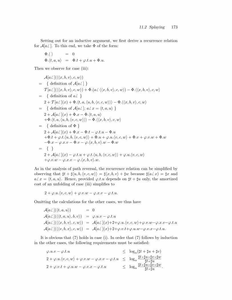
11.2 Splaying 173
Setting out for an inductive argument, we first derive a recurrence relationfor A[a6 ]. To this end, we take Φ of the form:
Φ.〈 〉 = 0Φ.〈t, a, u〉 = Φ.t+ ϕ.t.u+ Φ.u.
Then we observe for case (iii):
A[a6 ](〈〈x, b, v〉, c, w〉)= definition of A[a6 ]
T [a6 ](〈〈x, b, v〉, c, w〉) + Φ.(a6 〈〈x, b, v〉, c, w〉)− Φ.〈〈x, b, v〉, c, w〉= definition of a6
2 + T [a6 ](x) + Φ.〈t, a, 〈u, b, 〈v, c, w〉〉〉 − Φ.〈〈x, b, v〉, c, w〉= definition of A[a6 ]; a6 x = 〈t, a, u〉
2 +A[a6 ](x) + Φ.x− Φ.〈t, a, u〉+Φ.〈t, a, 〈u, b, 〈v, c, w〉〉〉 − Φ.〈〈x, b, v〉, c, w〉
= definition of Φ 2 +A[a6 ](x) + Φ.x− Φ.t− ϕ.t.u− Φ.u+Φ.t+ ϕ.t.〈u, b, 〈v, c, w〉〉+ Φ.u+ ϕ.u.〈v, c, w〉+ Φ.v + ϕ.v.w + Φ.w−Φ.x− ϕ.x.v − Φ.v − ϕ.〈x, b, v〉.w − Φ.w
= 2 +A[a6 ](x)− ϕ.t.u+ ϕ.t.〈u, b, 〈v, c, w〉〉+ ϕ.u.〈v, c, w〉+ϕ.v.w − ϕ.x.v − ϕ.〈x, b, v〉.w.
As in the analysis of path reversal, the recurrence relation can be simplified byobserving that ]t + ]〈u, b, 〈v, c, w〉〉 = ]〈x, b, v〉 + ]w because ](a6 x) = ]x anda6 x = 〈t, a, u〉. Hence, provided ϕ.t.u depends on ]t + ]u only, the amortizedcost of an unfolding of case (iii) simplifies to
2 + ϕ.u.〈v, c, w〉+ ϕ.v.w − ϕ.x.v − ϕ.t.u.
Omitting the calculations for the other cases, we thus have
A[a6 ](〈t, a, u〉) = 0A[a6 ](〈〈t, a, u〉, b, v〉) = ϕ.u.v − ϕ.t.u
A[a6 ](〈〈x, b, v〉, c, w〉) = A[a6 ](x)+2+ϕ.u.〈v, c, w〉+ϕ.v.w−ϕ.x.v−ϕ.t.uA[a6 ](〈〈v, b, x〉, c, w〉) = A[a6 ](x)+2+ϕ.v.t+ϕ.u.w−ϕ.v.x−ϕ.t.u.
It is obvious that (7) holds in case (i). In order that (7) follows by inductionin the other cases, the following requirements must be satisfied:
ϕ.u.v − ϕ.t.u ≤ logα(]t+ ]u+ ]v)
2 + ϕ.u.〈v, c, w〉+ ϕ.v.w − ϕ.x.v − ϕ.t.u ≤ logα]t+]u+]v+]w
]t+]u
2 + ϕ.v.t+ ϕ.u.w − ϕ.v.x− ϕ.t.u ≤ logα]t+]u+]v+]w
]t+]u .

174 Chapter 11 Path reversal, splaying, and pairing
To remove logα from these requirements, we define
ϕ.t.u = β logα(]t+ ]u),
with β > 0. The requirements then reduce to(]u+]v]t+]u
)β
≤ ]t+ ]u+ ]v
α2
(]u+]v+]w]t+]u+]v
]v+]w]t+]u
)β
≤ 1 + ]v+]w]t+]u
α2
(]v+]t
]v+]t+]u]u+]w]t+]u
)β
≤ 1 + ]v+]w]t+]u .
As constraints on α and β we thus have: α > 1, β > 0, and
(∀ k, l,m :: (l +m
k + l)β ≤ k + l +m)(8)
(∀ k, l,m, n :: α2(l +m+ n
k + l +m
m+ n
k + l)β ≤ 1 +
m+ n
k + l)(9)
(∀ k, l,m, n :: α2(k +m
k + l +m
l + n
k + l)β ≤ 1 +
m+ n
k + l).(10)
Under these constraints, we want to maximize α and, with lower priority, wewant to minimize β so as to keep Φ small.
We distinguish two cases.
Case β < 12 . Lemma 11.5 at the end of this section states that for 0 < β < 1
2 :
(8) ≡ β ≤ 1
(9) ≡ α2 ≤ (1−β)1−β
ββ(1−2β)1−2β
(10) ≡ α2 ≤ 4β,
so, taking the conjunction of the requirements on α and β, we obtain:
1 < α2 ≤ (1−β)1−β
ββ(1−2β)1−2βmin 4β
0 < β <12.
To maximize α, we determine the maximum of its upper bound over all β sat-isfying 0 < β < 1
2 . This yields 3√
4 as maximal value for α2 for β = 13 (see
Figure 11.3).
Case β ≥ 12 . Instantiation of (9) with “k, l,m, n := 1, 1, 1,∞” yields that
α2 ≤√
32 .
Since√
32 <
3√
4, we conclude from this case analysis that the optimal valuesfor α and β are given by α = 3
√2 and β = 1
3 .

11.2 Splaying 175
2
1
1/3
2
1
1/20
Figure 11.3: Maximum at β = 13 .
As result for the amortized costs of splaying we thus have (cf. (7)):
A[a6 ](x) ≤ 1 + 3 log2 ]x.
Furthermore, we have derived the following potential:
Φ.〈 〉 = 0Φ.〈t, a, u〉 = Φ.t+ log2 ]〈t, a, u〉+ Φ.u.
Note that Φ.x is Ω(]x log ]x) if each node of x has at most one nonempty sub-tree. It would be interesting to know whether there exists a linear potential forsplaying; this question will be addressed in Section 11.4.
We end this section with two remarks and the promised lemma.
Remark 11.3The remaining alternative for (iii) mentioned in Section 11.2.2,
a6 〈〈x, b, v〉, c, w〉 = 〈t, a, 〈〈u, b, v〉, c, w〉〉 |[ 〈t, a, u〉 = a6 x ]| , a<b<c,
drops out because it gives rise to constraint
(∀ k, l,m, n :: α2(l +m+ n
k + l +m
l +m
k + l)β ≤ 1 +
m+ n
k + l).
This implies that α ≤ 1 if we instantiate it with “k, l,m, n := 1,∞, 1, 1”, whichconflicts with α > 1.2
Remark 11.4The maximal value of (1−β)1−β
ββ(1−2β)1−2β turns out to be φ =√
5+12 , the golden ratio
again (for β = 5−√
510 (≈ 0.276)). So, if it were only for case (iii), constant 3 in
the bound for A[a6 ] could be replaced by 2/log2 φ (≈ 2.88).2

176 Chapter 11 Path reversal, splaying, and pairing
Lemma 11.5For 0 < β < 1
2 ,
(a) (∀ k, l,m ::(l+mk+l
)β
≤ k + l +m) ≡ β ≤ 1
(b) (∀ k, l,m, n :: α2(l+m+nk+l+m
m+nk+l
)β
≤ 1 +m+nk+l
) ≡ α2 ≤ (1−β)1−β
ββ(1−2β)1−2β
(c) (∀ k, l,m, n :: α2(
k+mk+l+m
l+nk+l
)β
≤ 1 +m+nk+l
) ≡ α2 ≤ 4β.
Proof The facts are proven by mutual implication.Proof of (a), using that β > 0:
(∀ k, l,m :: ( l+mk+l )β ≤ k + l +m)
⇐ β > 0 (∀ k, l,m :: (k+l+m
k+l )β ≤ k+l+mk+l )
≡ β ≤ 1;
(∀ k, l,m :: ( l+mk+l )β ≤ k + l +m)
⇒ take k = 1 and l = 1 (∀m :: (m+1
2 )β ≤ m+ 2)
⇒ take m→∞ β ≤ 1.
Proof of (b), using that 0 < β < 12 :
(∀ k, l,m, n :: α2( l+m+nk+l+m
m+nk+l )β ≤ 1 + m+n
k+l )
⇐ β > 0 (∀ k, l,m, n :: α2(k+l+m+n
k+lm+nk+l )β ≤ 1 + m+n
k+l )
≡ p = m+nk+l
(∀ p : p > 0 : α2((1+p)p)β ≤ 1 + p)
≡
(∀ p : p > 0 : α2 ≤ (1+p)1−β
pβ )
≡ minimize (1+x)1−β
xβ , using 0 < β < 12 (see below)
α2 ≤ (1−β)1−β
ββ(1−2β)1−2β ;

11.2 Splaying 177
(∀ k, l,m, n :: α2( l+m+nk+l+m
m+nk+l )β ≤ 1 + m+n
k+l )⇒ take k = m = 1
(∀ l, n :: α2( l+n+1l+2
n+1l+1 )β ≤ 1 + n+1
l+1 )≡
(∀ l, n :: α2 ≤ (1 + n+1l+1 )( l+2
l+n+1l+1n+1)β)
⇒ take nl →
β1−2β and l→∞ ( β
1−2β > 0, since 0 < β < 12)
α2 ≤ (1 + β1−2β )( 1
1+ β1−2β
1−2ββ )β
≡ 1 + β1−2β = 1−β
1−2β
α2 ≤ 1−β1−2β (1−2β
1−β1−2β
β )β
≡
α2 ≤ (1−β)1−β
ββ(1−2β)1−2β .
To complete the proof of this part, we minimize f(x) = (1+x)1−β
xβ over all x > 0.Then f ′(x) = 0 is equivalent to (1 − β)x = (1 + x)β, and f turns out to beminimal at β
1−2β , which is positive because 0 < β < 12 . So the minimum of f
equals(1+ β
1−2β)1−β
( β1−2β
)β, which in turn equals (1−β)1−β
ββ(1−2β)1−2β , since 1 + β1−2β = 1−β
1−2β .
Proof of (c), using that 0 < β < 12 :
(∀ k, l,m, n :: α2( k+mk+l+m
l+nk+l )
β ≤ 1 + m+nk+l )
⇐ β > 0 (∀ k, l,m, n :: α2(k+m
k+ll+nk+l )
β ≤ 1 + m+nk+l )
≡ p = k+mk+l and q = l+n
k+l (∀ p, q : p > 0 ∧ q > 0 ∧ p+ q ≥ 1 : α2(pq)β ≤ p+ q)
≡ (∀ p, q : p > 0 ∧ q > 0 ∧ p+ q ≥ 1 : α2 ≤ p+q
(pq)β)
≡ minimize x+y
(xy)β, using 0 < β < 1
2 (see below)
α2 ≤ 4β;
(∀ k, l,m, n :: α2( k+mk+l+m
l+nk+l )
β ≤ 1 + m+nk+l )
⇒ take l = k and m = n = 1 (∀ k :: α2( k+1
2k+1k+12k )β ≤ 1 + 2
2k )≡
(∀ k :: α2 ≤ (1 + 1k )(2k+1
k+12k
k+1)β)⇒ take k →∞
α2 ≤ 4β.

178 Chapter 11 Path reversal, splaying, and pairing
We determine the minimum of x+y
(xy)βover all positive x and y satisfying x+y ≥ 1.
To this end, we first observe that x+y
(xy)βtakes its minimal value only if x = y
because (xy)β is maximized by taking x equal to y (β > 0), and this can beachieved without changing the value of x + y. We thus minimize 2x1−2β overall x ≥ 1
2 . Since this function is increasing in x (β < 12), it attains its minimal
value of 4β at x = 12 .
2
11.2.4 Bounds for splay trees
Cost measure T has been chosen such that T [a6 ](x) is (as good as equal to) thenumber of comparisons needed to locate a in x (cf. program f in Remark 11.2).This measure corresponds to Sleator and Tarjan’s measure in [29]. The amor-tized costs satisfy
A[empty] is O(1)A[isempty](x) is O(1)A[member](a, x) ≤ 3 log2(1+#[[x]]) +O(1) comparisonsA[insert](x, a) ≤ 4 log2(1+#[[x]]) +O(1) comparisonsA[delete](x, a) ≤ 6 log2(1+#[[x]]) +O(1) comparisons.
For potential Φ we have as bounds
0 ≤ Φ.x ≤ (1+#[[x]]) log2(1+#[[x]]).
11.3 Pairing
In [7], Fredman, Sedgewick, Sleator, and Tarjan propose pairing heaps as practi-cal alternative for Fibonacci heaps. The central operation of this data structure,called pairing, transforms a list of heaps into a single heap by repeatedly linkingtwo heaps in a specific order. In this section we consider one of the numerousvariants of pairing, viz. the so-called two-pass variant.
11.3.1 Pairing heaps
Pairing heaps can be used to implement the following algebra of priority queues,which is about the same as algebra PQ′ from Chapter 10:
PQ′′ = ( Int | , (= ), ·, ·∪, ↓,⇓, deckey ).
As signature for the implementation of this algebra we use
PH = (P | empty, isempty, single, union,min, delmin, deckey ).
Characteristic of pairing heaps is that P is a subset of tree type

11.3 Pairing 179
〈Int〉9 = 〈 〉 ∪ 〈Int〉4,
where type 〈Int〉4 has been defined in Section 6.3.1 as the smallest solution of
X : X = Int× [X].
Note that for a tree 〈a, t〉 in 〈Int〉9, the trees in t are nonempty—as they areelements of 〈Int〉4. Data type P is now, informally, defined as the set of trees oftype 〈Int〉4 that are free of duplicates and satisfy the heap condition.
Again, the fundamental operation on heaps is linking, which is defined ontrees of type 〈Int〉9 by
〈 〉 1 y.= y
x 1 〈 〉 .= x〈a, t〉 1 〈b, u〉 .= 〈a, 〈b, u〉 ` t〉 , a < b
〈b, 〈a, t〉 `u〉 , b < a.
In terms of this operator, the operations of PH are defined as follows:
empty.= 〈 〉
isempty.x.= x = 〈 〉
single.a.= 〈a, [ ]〉
union.x.y.= x1 y
min.〈a, t〉 .= a
delmin.〈a, t〉 .= cp.t.
Function cp transforms a list of heaps into a single heap by repeatedly linkingtwo heaps. This can be done in many ways. The method analyzed in [7] isthe two-pass variant: in the first pass, heaps are linked pairwise from left toright; in the second pass, the resulting heaps are combined from right to left.These two passes are concisely encoded in the following program for cp (“pairand combine”, or “pairing” for short).
cp.[ ] = 〈 〉cp.[x] = x
cp.(x` y ` t) = (x1 y) 1 cp.t.
Note that the cost of pairing is charged to the applications of 1 .To program deckey, we use the following root-path view of 〈Int〉9:
[ [〈Int〉9]× Int× [〈Int〉9] ]× 〈Int〉9,
which corresponds to root-path view 〈T 〉8 of tree type 〈T 〉4 from Section 6.3.2.In terms of this type, deckey is programmed as follows:
deckey.a.k.(z, 〈a, t〉) .= z1 〈a−k, t〉,

180 Chapter 11 Path reversal, splaying, and pairing
where we have abbreviated (z, 〈 〉) to z, and ([ ], 〈a−k, t〉) to 〈a−k, t〉.The cost measure defined by the dots in the above programs will be called T .
As for the complexity of these operations, it is still an open problem whether theamortized cost of deckey is O(1). In the next section, we derive a logarithmicbound for the amortized cost of cp. The potential function obtained in thisanalysis yields a logarithmic bound for deckey.
11.3.2 Analysis of pairing
We use ]t to denote #〈a, t〉, hence ]t is positive for all lists t. The goal of theanalysis of cp is to maximize α such that α > 1 and
A[cp](t) ≤ logα ]t,(11)
where A[cp](t) denotes the amortized cost of pairing, defined by
A[cp](t) = T [cp](t) + Φ.(cp.t)− Φ.t.
Note that cp.t is a tree of type 〈Int〉9, whereas t is a list of type [〈Int〉9]. PotentialΦ is therefore defined both on 〈Int〉9 and [〈Int〉9]:
Φ.〈 〉 = 0Φ.〈a, t〉 = ϕ.t+ Φ∗.t
Φ.t = ϕ.t+ Φ∗.t, with Φ∗.t = (Σx : x ∈ t : Φ.x).
Hence, Φ.〈a, t〉 = Φ.t. To achieve that Φ is nonnegative, we require ϕ to benonnegative. In terms of the amortized costs of linking, given by
A[1 ](x, y) = T [1 ](x, y) + Φ.(x1 y)− Φ.x− Φ.y,
the following recurrence relation can now be derived from the program for cp:
A[cp]([ ]) = −ϕ.[ ]A[cp]([x]) = −ϕ.[x]A[cp](x` y ` t) = A[1 ](x, y) +A[1 ](x1 y, cp.t)− ϕ.(x` y ` t) + ϕ.t
+A[cp](t),
using that Φ.(x` y ` t) = ϕ.(x` y ` t) + Φ.x+ Φ.y + Φ.t− ϕ.t.Since ϕ will be nonnegative, (11) evidently holds if t = [ ] or t = [x]. It
follows by induction in the remaining case, provided
A[1 ](x, y) +A[1 ](x1 y, cp.t)− ϕ.(x` y ` t) + ϕ.t ≤ logα](x` y ` t)
]t .(12)
To simplify this requirement on ϕ, we investigate A[1 ]. For x = 〈a, t〉 andy = 〈b, u〉 we observe for the case a < b:

11.3 Pairing 181
A[1 ](x, y)
= definition of A[1 ] T [1 ](x, y) + Φ.(x1 y)− Φ.x− Φ.y
= definitions of 1 and T 1 + Φ.〈a, y ` t〉 − Φ.〈a, t〉 − Φ.y
= definition of Φ and Φ∗ 1 + ϕ.(y ` t) + Φ.y + Φ∗.t− ϕ.t− Φ∗.t− Φ.y
= 1 + ϕ.(y ` t)− ϕ.t.
Introducing
δ.(y ` t) = ϕ.(y ` t)− ϕ.t,(13)
we then have on account of symmetry
A[1 ](x, y) = 1 +
δ.(y ` t) , a < bδ.(x`u) , b < a.
To avoid the case analysis in this result we let δ.t depend on ]t only. Definingδ.〈a, t〉 = δ.t, we then have
A[1 ](x, y) = 1 + δ.(x1 y),(14)
since both ](y ` t) and ](x`u) are equal to #(x1 y).In terms of δ, requirement (12) becomes:
2 + δ.(x1 y) + δ.((x1 y) 1 cp.t)− δ.(x` y ` t)− δ.(y ` t) ≤ logα#x+#y+]t
]t .(15)
As in the previous analyses in this chapter we take
δ.t = β logα ]t,
and to achieve that ϕ is nonnegative we also take ϕ.[ ] = 0, which defines ϕ onaccount of (13).
Using that #(cp.t) = ]t− 1, requirement (15) then reduces to:
α2(
#x+ #y + ]t− 1#x+ #y + ]t
#x+ #y
#y + ]t
)β
≤ 1 +#x+ #y
]t.
In summary, we thus have that (11) holds and that Φ is nonnegative providedα and β satisfy: α > 1, β > 0, and
(∀ k,m, n :: α2(m+ n+ k − 1m+ n+ k
m+ n
n+ k
)β
≤ 1 +m+ n
k).(16)

182 Chapter 11 Path reversal, splaying, and pairing
Since m+n+k−1m+n+k is about 1, this set of requirements is very similar to the one in
the analysis of path reversal. To maximize α, we distinguish two cases.
Case β < 1. Since constraint (16) is about equal to constraint (4) in the analysisof path reversal, we omit the calculations that lead to the following constraintson α and β:
1 < α2 ≤ 1ββ(1− β)1−β
0 < β < 1.
The optimal values thus are α =√
2 and β = 12 .
Case β ≥ 1. Instantiating (16) with “k,m, n := 1,∞, 1” yields that α2 ≤ 2,hence α ≤
√2.
We conclude that the optimal values are α =√
2 and β = 12 . As result for
A[cp] we thus have (on account of (11)):
A[cp](t) ≤ 2 log2 ]t,
for potential Φ defined by
Φ.〈 〉 = 0Φ.〈a, t〉 = Φ.tΦ.[ ] = 0Φ.(x` t) = Φ.x+ log2 ](x` t) + Φ.t.
11.3.3 Bounds for pairing heaps
To analyze the respective operations we recall the following result of the previoussection (cf. (14)):
Φ.(x1 y)− Φ.x− Φ.y = log2 #(x1 y).(17)
This yields for the first six operations:
A[empty] is O(1)A[isempty](x) is O(1)A[single](a) is O(1)A[union](x, y) ≤ log2 #[[union.x.y]] comparisonsA[min](x) is O(1)A[delmin](x) ≤ 2 log2 #[[x]] comparisons.
These bounds imply that sorting N numbers by means of pairing heaps requiresasymptotically at most 2N log2N comparisons, instead of 2.88N log2N for Fi-bonacci heaps.
To analyze deckey we must be a little careful. We use the property that

11.4 Why these “sum of logs” potentials? 183
Φ.(z, 〈a, t〉) ≥ Φ.z + Φ.〈a, t〉.
Then we observe, writing x = (z, 〈a, t〉):
A[deckey](a, k, x)
= definition of A[deckey] T [deckey](a, k, x) + Φ.(deckey.a.k.x)− Φ.x
= definitions of T and deckey 1 + Φ.(z1 〈a−k, t〉)− Φ.(z, 〈a, t〉)
≤ above property 1 + Φ.(z1 〈a−k, t〉)− Φ.z − Φ.〈a, t〉
= (17), using Φ.〈a, t〉 = Φ.〈a−k, t〉 1 + log2 #x.
Let us briefly compare pairing heaps with Fibonacci heaps. Between datatype P and data type F defined in Section 10.3, we observe three major differ-ences: (a) F consists of trees over Int × [0..K] whereas trees in P are over Int,(b) trees in P can have any structure whereas trees in F are pseudo-binomial,and (c) the order of the subtrees is taken into account for trees in P , while it isirrelevant for trees in F (compare tree types 〈T 〉4 and 〈T 〉6).
Because of these differences, Fibonacci heaps are not as “self-adjusting” [7] aspairing heaps are. Combined with the fact that the implementation at pointerlevel is simpler and more space efficient, this makes pairing heaps interestingfrom a practical point of view. From a theoretical point of view, however,Fibonacci heaps are to be preferred because the amortized costs of deckey havebeen shown to be O(1).
11.4 Why these “sum of logs” potentials?
For path reversal, splaying, and pairing, we have derived the following potentialfunctions:
Φ.〈a, t〉 = 12 log2 #〈a, t〉+ (Σx : x ∈ t : Φ.x),
Φ.〈 〉 = 0Φ.〈t, a, u〉 = Φ.t+ log2 ]〈t, a, u〉+ Φ.u,
and
Φ.〈 〉 = 0Φ.〈a, [ ]〉 = 0Φ.〈a, x` t〉 = Φ.x+ log2 #〈a, x` t〉+ Φ.〈a, t〉.

184 Chapter 11 Path reversal, splaying, and pairing
For these potential functions, the contribution of each node to the potential ofthe tree is proportional to the logarithm of the size of its subtrees. (In case ofpairing, 〈a, x` t〉 can be viewed as a node with left subtree x and right subtree〈a, t〉.) The fact that these “sum of logarithms” potentials serve to analyzeboth splaying and pairing is easy to explain, since there is a clear connectionbetween these two operations (see [7, p.121]). But the authors of [12] are at aloss to explain that such a potential can also be used to amortize the cost ofpath reversal, because they cannot discover a connection between splaying (andpairing) on the one hand, and path reversal on the other hand. To us, however,this fact is not a surprise anymore because we are able to analyze these threeoperations in the same systematic way.
In connection with the amortized complexity of deckey for pairing heaps, animportant question is whether a smaller potential than “sum of logs” is possible.Since A[deckey](a, k, x) ≤ 1+δ.x, we would obtain a better bound if we were ableto show that, for instance, δ.x = log log ]x is possible. Unfortunately, however,a smaller potential cannot be obtained in our analyses of path reversal, splaying,and pairing, as we will now show for path reversal.
In the bottom-up analysis of path reversal, we defined ψ.t = ]t, and thischoice for ψ led to requirement (4) on α and β. To investigate whether a smallerchoice for ψ.t is possible, e.g. ψ.t = log ]t, we introduce a function f on thepositive integers, and take ψ.t = β
√f.]t. As requirement on f we then obtain
formula (18) in the lemma below. In our analysis we have chosen f.n =√n (for
α = 2 and β = 12). Lemma 11.6 shows that f cannot be substantially smaller.
Lemma 11.6Let f be a function defined on the positive integers such that f.n ≥ 1. Supposef satisfies
(∀m,n ::f.m
f.n≤ m+ n
αn),(18)
for some α > 1. Then f.n is Ω(nε) and O(n1−ε), with 0 < ε < 12 .
Proof For a sufficiently large integer c, we instantiate (18) with m,n := c n, nand m,n := n, c n, respectively. This yields that, for all positive n:
f.(cn)f.n
≤ c+ 1α
∧ f.n
f.(cn)≤ 1 + c
αc,
or, equivalently,
αc
c+ 1≤ f.(cn)
f.n≤ c+ 1
α.
Since α ≤ 2 (instantiate (18) with m = n), the lower bound does not exceed theupper bound (using 4c ≤ (c+1)2). We take c > 1
α−1 (hence c > 1), and define
ε = logcαc
c+1 .

11.4 Why these “sum of logs” potentials? 185
Then 0 < ε < 12 , and for all positive n:
cε ≤ f.(cn)f.n
≤ c1−ε.
From these inequalities we deduce, by induction on k, that
ckε ≤ f.(ckn)f.n
≤ ck(1−ε),
for all k ≥ 0, from which we conclude that f.n is Ω(nε) and O(n1−ε), with0 < ε < 1
2 .2
Along the same lines it can be shown that a potential which is substantiallysmaller than a “sum of logs” potential cannot be used in our analyses of splayingand pairing. For pairing the argument is as follows. The counterpart of (18),corresponding to requirement (16) on ϕ, is
(∀ k,m, n ::f.(m+ n+ k − 1)f.(m+ n+ k)
f.(m+ n)f.(n+ k)
≤ m+ n+ k
α2k).
Taking n = 1, this implies
(∀ k,m ::f.(m+ k)
f.(m+ k + 1)f.(m+ 1)f.(k + 1)
≤ m+ k + 1α2k
).
Since m+ k ≈ m+ k + 1, this formula is similar to (18); therefore, f.n is againΩ(nε) and O(n1−ε), with 0 < ε < 1
2 .The moral thus is that a better bound for A[deckey] can only be obtained
by using more complex potential functions—if at all possible. It is, for instance,conceivable that a potential takes the depth of the nodes into account; for ex-ample, a suitable potential for a tree x might be Φ.0.x, with
Φ.k.〈 〉 = 0Φ.k.〈t, a, u〉 = Φ.(k+1).t+ ϕ.k.t.u+ Φ.(k+1).u
Whether such potentials exist is an open problem.

186
Chapter 12
Conclusion
The original incentive that led to the research which culminated in this thesiswas to increase our understanding of amortized complexity, in particular ourinsight in the nature of potential functions. To achieve this we have tried toderive potentials as systematically as possible for a number of data structures.The only paper we know of in which this is also an explicit goal is by Nelson [26],who derives a potential to show that snoopy caching is efficient in the amortizedsense. Other work along the lines of this thesis has been recorded in [15, 18].Furthermore, Sleator has recently shown how potentials can be computed bymeans of linear programming [28]. The examples in his paper, however, arerestricted to operations whose amortized costs are bounded by a constant; datastructures like skew heaps and splay trees are not covered.
A key factor to successful analysis of data structures is the description of theoperations at the right level of detail. Our experience is that a functional pro-gramming style combined with the appropriate choice of list and tree types leadsto concise programs which capture the essence of the operations. An importantaspect is that these programs are recursive, which leads to recurrence relationsfor the actual costs as well as the amortized costs. The recurrence relations forthe amortized costs are formulated in terms of a potential function, and usingmathemathical induction a potential function can so be derived. Also, we haveshown how the use of top-down simulations (read “algorithmic refinements”) ofbottom-up operations like bottom-up melding and path reversal simplifies theanalysis of such operations.
In Part I we introduced the necessary tools needed to specify and (re)designseveral (mostly existing) data structures in Part II in an effective way. Weobtained concise descriptions of these data structures and our analyses resultedin bounds that either matched or improved upon existing bounds. There aremany directions in which the research reported in this thesis can be extended.Below we mention a few.
1. In Chapter 2 the notion of algebra refinement has been defined for monoal-gebras only. Starting from a notion of data refinement of relations (or—perhaps better—monotonic predicate transformers), this definition may

Conclusion 187
be extended to a more general notion of algebra refinement. In this way,nondeterministic operations that, for instance, arbitrarily pick an elementfrom a given set can be dealt with as well.
2. In Chapter 3 we have shown that any amortized analysis can be donein terms of a potential function. Some well-known data structures, suchas solutions to the union-find problem (see, e.g., [32]), are only analyzedby means of the banker’s method. It is interesting to look what the po-tential functions for these data structures look like. In particular, it isinteresting to find the potential that corresponds to the banker’s analy-sis of path reversal of Tarjan and van Leeuwen (proof of Lemma 10 in[32]) and to compare it to our analysis in Chapter 11 (where it should benoted that our analysis only gives an O((n+m) log n) bound instead onthe O(n+m log n) bound in [32] for the cost of m reversals on an arbitraryinitial n-node tree).
3. At the end of Chapter 10 we have seen that the fact that the numberof deckey operations on each node is bounded by a constant K, say,gives rise to more efficient implementations. Moreover, in Section 9.4.4(Lemma 9.12) we have shown that depending on the ratio of the numberof union’s and the number of delmin’s different bounds for the amortizedcosts of these operations are obtained. The question is now how to de-scribe additional knowledge about the use of the operations of an algebrain a formal and convenient way.
4. In Chapter 9 we conjectured that the “logφ” bound for top-down meld-ing is tight. To confirm this conjecture a worst-case sequence of meldingoperations must be constructed, which turns out to be rather difficult. Aweaker—but nevertheless interesting—result would be whether the boundin Lemma 9.2 is tight for the particular potential function defined in thislemma.
5. Yet another question is under which circumstances amortized efficient datastructures can be used in an efficient way in parallel programs. The prob-lem is that a slow operation in one process may suspend several otherprocesses due to delayed communications, which may affect the perfor-mance drastically.
Finally, to put our work in perspective, we would like to stress that weconsider our quite formal approach complementary to the more intuitively basedapproaches of algorithm design. The latter led to new and surprising results,whereas the former can be used to polish up known results, but also to achievenew results—as we have shown in this thesis.

188
References
1. Aho A.V., Hopcroft J.E., Ullman J.D. The Design and Analysis of Com-puter Algorithms. Addison-Wesley (1974).
2. Back R.-J.R. Correctness preserving program refinements: proof theory andapplications. Mathematical Centre Tracts 131, Department of ComputerScience, Mathematisch Centrum, Amsterdam (1980).
3. Bird R.S. Lectures on Constructive Functional Programming. Technicalmonograph PRG 69, Oxford University Computing Laboratory (1988).
4. Chen W., Udding J.-T. Towards a calculus of data refinement. In: J.L.A.v.d. Snepscheut (ed.), Mathematics of Program Construction, LNCS 375,Springer-Verlag (1989) 197–218.
5. Dijkstra E.W. A Discipline of Programming. Prentice-Hall (1976).6. Dijkstra E.W., Scholten C.S. Predicate Calculus and Program Semantics.
Springer-Verlag (1990).7. Fredman M.L., Sedgewick R., Sleator D.D., Tarjan R.E. The pairing heap:
a new form of self-adjusting heap. Algorithmica 1 (1986) 111–129.8. Fredman M.L., Tarjan R.E. Fibonacci heaps and improved network opti-
mization algorithms. Journal of the ACM 34 (1987) 596–615.9. Gabow H.N., Bentley J.L., Tarjan R.E. Scaling and related techniques for
geometry problems. Proceedings of the 16th Annual ACM Symposium onTheory of Computing (1984) 135–143.
10. Gajewska H., Tarjan R.E. Deques with heap order. Information ProcessingLetters 22 (1986) 197–200.
11. Gardiner P.H.B., Morgan C.C. Data refinement of predicate transformers.Theoretical Computer Science 87 (1991) 143–162.
12. Ginat D., Sleator D.D., Tarjan R.E. A tight amortized bound for pathreversal. Information Processing Letters 31 (1989) 3–5.
13. Gries D. The Science of Programming. Springer-Verlag (1981).14. Hagerup T. On saving space in parallel computation. Information Process-
ing Letters 29 (1988) 327–329.15. Heutinck R. Priority queues. Master’s thesis (in Dutch), Department of
Mathematics and Computing Science, Eindhoven University of Technology(1989).
16. Hoare C.A.R. Proof of correctness of data representations. Acta Informat-ica 1 (1972) 271–281.

References 189
17. Hoogerwoord R.R. The design of functional programs: a calculational ap-proach. Ph.D. thesis, Department of Mathematics and Computing Science,Eindhoven University of Technology (1989).
18. Hurk P.A.J.M. v.d. Het ontwerpen van geamortiseerd efficiente data-structuren. Master’s thesis (in Dutch), Department of Mathematics andComputing Science, Eindhoven University of Technology (1989).
19. Italiano G.F. Amortized efficiency of a path retrieval data structure. The-oretical Computer Science 48 (1986) 273–281.
20. Kaldewaij A. Programming: The Derivation of Algorithms. Prentice-Hallinternational series in computer science (1990).
21. Kaldewaij A., Schoenmakers B. The derivation of a tighter bound for top-down skew heaps. Information Processing Letters 37 (1991) 265–271.
22. McCreight E.M. Pagination of B∗-trees with variable-length records. Com-munications of the ACM 20 (1977) 670–674.
23. Mehlhorn K. Data Structures and Algorithms 1: Sorting and Searching.Springer-Verlag (1984).
24. Mehlhorn K., Tsakalidis A. Data Structures. In: J. van Leeuwen (ed.),Handbook of Theoretical Computer Science, Chapter 6, Elsevier SciencePublishers B.V. (1990) 301–341.
25. Morris J. Laws of data refinement. Acta Informatica 26 (1989) 287–308.26. Nelson G. Methodical competitive snoopy-caching. In: W.H.J. Feijen,
A.J.M. v. Gasteren, D. Gries, J. Misra (eds.), Beauty is our business:a birthday tribute to Edsger W. Dijkstra, Chapter 38, Springer-Verlag(1990) 339–345.
27. Peyton Jones S.L. The Implementation of Functional Programming Lan-guages. Prentice-Hall international series in computer science (1987).
28. Sleator D.D. Data structures and terminating Petri nets. In: I. Simon(ed.), Latin’92, LNCS 583, Springer-Verlag (1992) 488–497.
29. Sleator D.D., Tarjan R.E. Self-adjusting binary search trees. Journal ofthe ACM 32 (1985) 652–686.
30. Sleator D.D., Tarjan R.E. Self-adjusting heaps. SIAM Journal on Com-puting 15 (1986) 52–69.
31. Tarjan R.E. Amortized computational complexity. SIAM Journal on Alge-braic and Discrete Methods 6 (1985) 306–318.
32. Tarjan R.E., Leeuwen J. v. Worst-case analysis of set union algorithms.Journal of the ACM 31 (1984) 245–281.
33. Turner D.A. SASL Language Manual. University of St. Andrews (1976).34. Vuillemin J. A data structure for manipulating priority queues. Commu-
nications of the ACM 21 (1978) 309–315.35. Vuillemin J. A unifying look at data structures. Communications of the
ACM 23 (1980) 229–239.36. Wadler P. Linear types can change the world! In: M. Broy, C.B. Jones
(eds.), Programming Concepts and Methods, North-Holland, Amsterdam(1990) 561–581.

190
Glossary of notation
∅ empty set, empty function, empty relation⊥ empty tuple⊥ unit typedomR , rngR domain, range of relation RR.x relation R applied to xyRx (x, y) ∈ RS R composition of relations R and SR? dual of relation RRX restriction of relation R to Xyfx x ∈ dom f ∧ y = f.x for function ff [x:=y] function f except that f [x:=y].x = yXyY partial functions from X to YX→Y (total) functions from X to Y?T arbitrary value of type TBool set of booleans, true, falseNat, Int,Real set of natural, integer, real numbersφ golden ratio (1 +
√5)/2
[a..b) interval x | a ≤ x < b[a..b] interval x | a ≤ x ≤ b(a..b] interval x | a < x ≤ b(a..b) interval x | a < x < bT,T
, [T ], 〈T 〉 finite structures over T#x size of structure xa ∈ x value a occurs in structure x↓x , ↑x minimum, maximum of structure xT finite sets over T , a empty set, singleton set a·∪ disjoint set unionS ⊕ a S ∪ a for a 6∈ SS a S \ a for a ∈ S⇓S S \ ↓S for nonempty set ST
finite bags (multisets) over T,a
empty bag, singleton bag a⇓B B↓B
for nonempty bag B , ⊕ bag subtraction, bag summation

Glossary of notation 191
[T ] finite lists over T[ ], [a] empty list, singleton list a` , hd, tl cons, head, taila , ft, lt snoc, front, last element++ (con)catenation#s length of list ss↑n prefix of length n of list ss↓n suffix of length #s− n of list ss.n (n+1)-st element of list srev.s reverse of list s〈T 〉 finite binary trees over T , (µX : 〈 〉 ∈ X : X×T×X)〈 〉 empty tree〈t, a, u〉 tree with left subtree t, root a, and right subtree u〈a〉 singleton tree a, 〈〈 〉, a, 〈 〉〉l.t,m.t, r.t left subtree, root (middle), and right subtree of tree t]t size of t plus one, ]〈 〉 = 1 and ]〈t, a, u〉 = ]t+ ]ut inorder traversal of tree t〈T 〉1 (µX :: [X × T ])〈T 〉2 (µX :: [X × T ∪ T ×X])〈T 〉3 [〈T 〉 × T ∪ T × 〈T 〉]× 〈T 〉〈T 〉4 (µX :: T × [X])〈T 〉5 (µX :: T ×
X)
〈T 〉6 (µX :: T × X)〈T 〉7 [〈T 〉6]〈T 〉8 [ [〈T 〉4]× T × [〈T 〉4] ]× 〈T 〉4' coupling relation[[·]] abstraction function([·]) representation functionrng A range of algebra Aval(E) value of expression ET ,N cost measuresT (E) cost of expression ET [f ] cost of function f.= unfolding counted by cost measure= unfolding counted twice by cost measureA[f ] amortized cost of function f†x rank of tree x‡x pseudo-rank of tree x1 top-down melding/linkingMO bottom-up meldinga6 path reversal/splaying at a

192
Index
abstract, 20, 24abstraction function, 29–30algebra, 12algebra refinement, 26algorithmic refinement, 22amortized analysis, 40–44, 47, 71–73amortized cost of function, 69arrays, 16, 96
bags, 11banker’s view, 42, 47benevolent side-effects, 61, 74bijective algebra, 35binary representation, 14, 68binary search trees, 168binary trees, 12, 87, 94binomial queues, 147binomial trees, 150booleans, 10, 13, 35
calculational style, 1Cartesian trees, 106circularly-linked list, 56composition rules, 64, 69concrete, 20, 24conservative analysis, 47cost measure, 64cost of function, 64coupling relation, 24, 26creation operation, 17
data refinement, 24data type, 12deques, 57, 75
with minimum, 106destructivity, 16, 54diagonal bags, 154dictionary, 167
distribution rules, 65–67distributive cost measure, 65doubly-linked list, 57
eager evaluation, 51
Fibonacci heaps, 146, 157first-order, 17–18, 49forests, 92fork, 58, 80, 81function, 10functional program, 20, 50, 53
golden ratio, 6, 144, 158, 175
higher-order, 19
infinite lists, 19injective algebra, 33, 107inorder traversal, 12inspection operation, 17intervals, 10
linear usage, 58, 62, 75linking, 149, 151, 157, 179lists, 11
meldingbottom-up, 127, 129, 144top-down, 113, 116, 122, 123, 143
monoalgebra, 17
numerical types, 10, 13
operation, 12
pairing, 179pairing heaps, 178, 182parameter patterns, 50, 84, 85, 89path reversal, 161

Index 193
physicist’s view, 42, 47pointers, 16, 52–54potential function, 42, 47, 69
sum of logs, 144, 165, 175, 182,183
priority queues, 16, 110, 146, 178program, 20
see also functional programprogram notation, 50–51, 53–54pseudo-binomial trees, 154pseudo-rank, 154purely-functional, 51
queues, 15, 55with minimum, 106
range of algebra, 32rank, 150relation, 9representation function, 29–30root-path views, 91, 93, 153, 156,
161, 170, 179
self-adjusting, 183sets, 11sharing, 52, 65signature, 27simulation, 132, 165singly-linked list, 53skew heaps
bottom-up, 127, 142top-down, 113–114, 122
skewed view, 88, 126sorting
bounds, 123, 139, 141, 151, 158,182
programsMergesort, 60PQsort, 123sort1, 111
specification, 21splay trees, 168, 178splaying, 168, 170–172stacks, 15, 50
destructive, 55, 58purely-functional, 53
with deletion, 86with minimum, 104
structures, 11subalgebra, 13surjective algebra, 32
transformation operation, 17trees, 92
see also binary treestuple, 9
unary representation, 13, 24, 31unfolding, 52unit type, 10
where-clause, 50without loss of efficiency, 15, 76, 78worst-case analysis, 67