data, statistics, probability 1 - unil statistics, probability 1.pdf · executive mba -hec lausanne...

Executive MBA - HEC Lausanne

2007/20081

Data, Statistics, Probability 1 :Describing data

Relationships between variables

Christopher Grigoriou


2007/20082

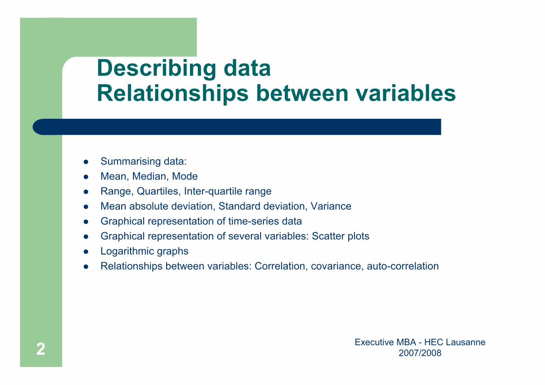
Describing dataRelationships between variables

� Summarising data:

� Mean, Median, Mode

� Range, Quartiles, Inter-quartile range

� Mean absolute deviation, Standard deviation, Variance

� Graphical representation of time-series data

� Graphical representation of several variables: Scatter plots

� Logarithmic graphs

� Relationships between variables: Correlation, covariance, auto-correlation


2007/20083

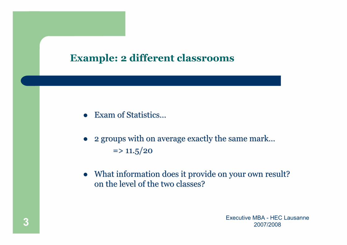
Example: 2 different classrooms

�� ExamExam ofof StatisticsStatistics……

�� 2 groups 2 groups withwith on on averageaverage exactlyexactly thethe samesame markmark……

=> 11.5/20=> 11.5/20

�� WhatWhat information information doesdoes itit provideprovide on on youryour ownown resultresult? ?

on on thethe levellevel ofof thethe twotwo classes?classes?


2007/20084

Class A

5.9σ11.5Mean

34.3Var.149.5Sum

72.258.511.52013

49711.518.512

30.255.511.51711

20.254.511.51610

12.253.511.5159

6.252.511.5148

0.250.511.5127

2.25-1.511.5106

6.25-2.511.595

20.25-4.511.574

30.25-5.511.563

72.25-8.511.532

90.25-9.511.521

(Xi-mean)²Xi-MeanMeanXiRank


2007/20085

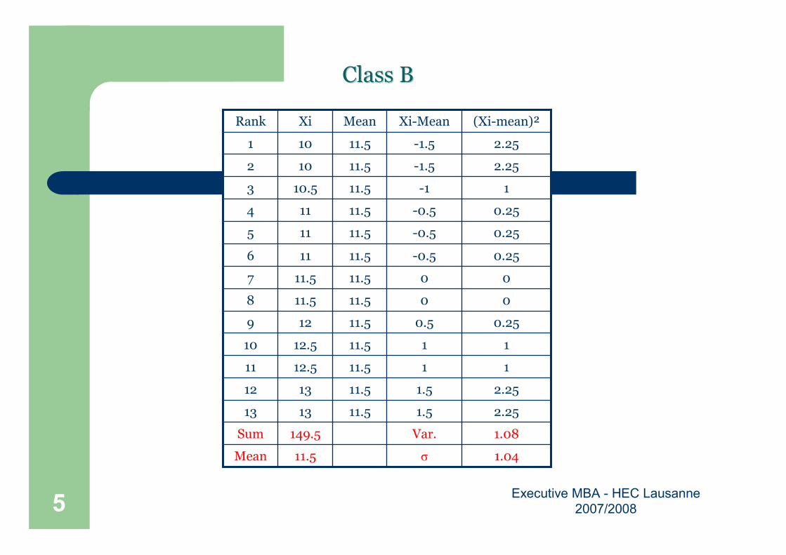
ClassClass BB

1.04σ11.5Mean

1.08Var.149.5Sum

2.251.511.51313

2.251.511.51312

1111.512.511

1111.512.510

0.250.511.5129

0011.511.58

0011.511.57

0.25-0.511.5116

0.25-0.511.5115

0.25-0.511.5114

1-111.510.53

2.25-1.511.5102

2.25-1.511.5101

(Xi-mean)²Xi-MeanMeanXiRank


2007/20086

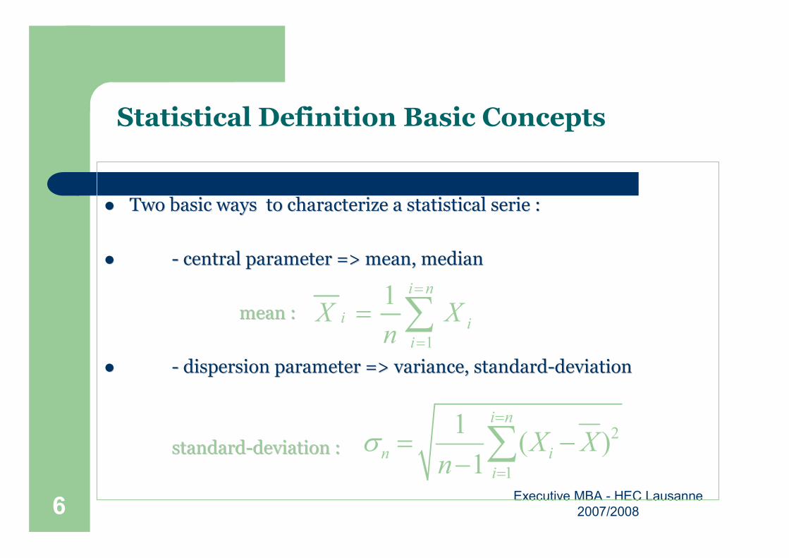
Statistical Definition Basic Concepts

�� TwoTwo basic basic waysways to to characterizecharacterize a a statisticalstatistical serieserie : :

�� -- central central parameterparameter => => meanmean, , medianmedian

meanmean ::

�� -- dispersion dispersion parameterparameter => variance, => variance, standardstandard--deviationdeviation

standardstandard--deviationdeviation ::

1

1 i n

ii

i

X Xn

=

=

= ∑

2

1

1( )

1

i n

n i

i

X Xn

σ=

=

= −−∑


2007/20087

=> To => To characterizecharacterize a a serieserie youyou needneed�� TheThe meanmean ofof thethe serieserie (central (central parameterparameter))

�� TheThe standardstandard--deviationdeviation (dispersion)(dispersion)

=>=>……ofof course, course, thethe answeranswer alsoalso dependsdepends

on on thethe dispersion (dispersion (standardstandard--deviationdeviation))


2007/20088

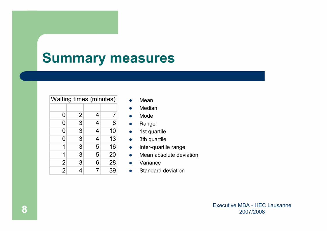
Summary measures

� Mean

� Median

� Mode

� Range

� 1st quartile

� 3th quartile

� Inter-quartile range

� Mean absolute deviation

� Variance

� Standard deviation

Waiting times (minutes)

0 2 4 7

0 3 4 8

0 3 4 10

0 3 4 13

1 3 5 16

1 3 5 20

2 3 6 28

2 4 7 39


2007/20089

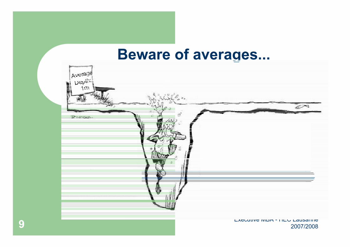
Beware of averages...


2007/200810

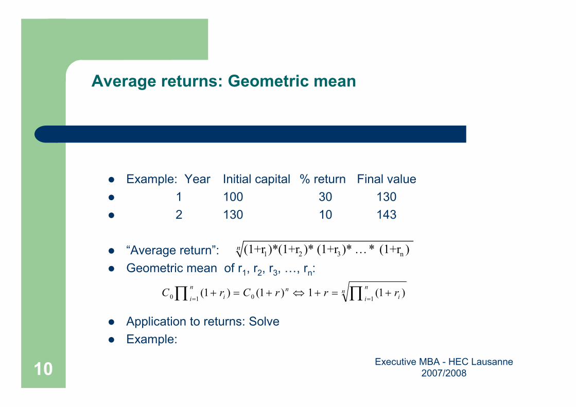
Average returns: Geometric mean

� Example: Year Initial capital % return Final value

� 1 100 30 130

� 2 130 10 143

� “Average return”:

� Geometric mean of r1, r2, r3, …, rn:

� Application to returns: Solve

� Example:

1 2 3 n(1+r )*(1+r )* (1+r )* * (1+r ) n …

nn

i i

nn

i irrrCrC ∏∏ ==

+=+⇔+=+1010 )1(1)1()1(


2007/200811

Data presentation: Accuracy

� Museum of prehistoric animals

Small boy to the curator: “Sir, how old is this dinosaur?”

Curator: ” 7,000,012 years old.”

Small boy: “Unbelievable, how can you be so accurate?”

Curator: “Well, it was 7 million when I started working at this museum, and I have been here 12

years.”

� In the lab

A physics student carried out an experiment to estimate a constant.

The true value of the constant was 0.0001342.

The student’s experiment yielded 0.0002411, a difference of only 0.0001069.

The student concluded that his experiment was a success.


2007/200812

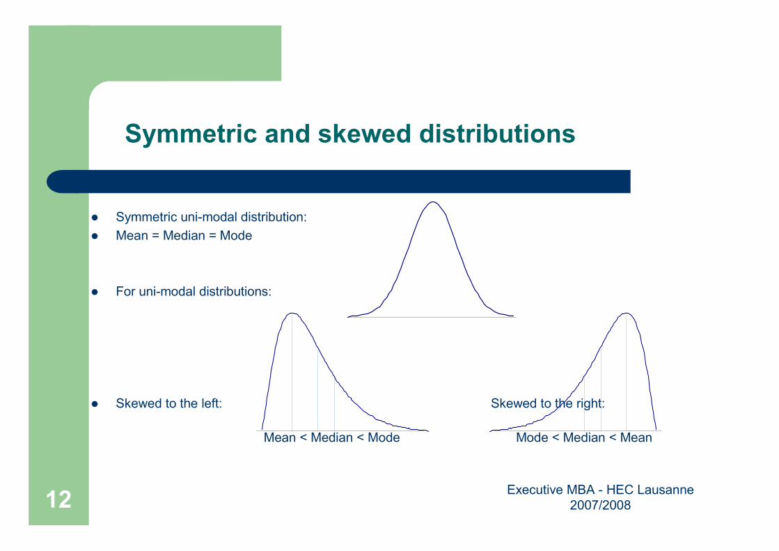
Symmetric and skewed distributions

� Symmetric uni-modal distribution:

� Mean = Median = Mode

� For uni-modal distributions:

� Skewed to the left: Skewed to the right:

Mean < Median < Mode Mode < Median < Mean


2007/200813

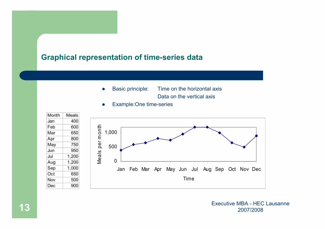
Graphical representation of time-series data

� Basic principle: Time on the horizontal axis

Data on the vertical axis

� Example:One time-series

Month Meals

Jan 400

Feb 600

Mar 650

Apr 800

May 750

Jun 950

Jul 1,200

Aug 1,200

Sep 1,000

Oct 650

Nov 500

Dec 900

0

500

1,000

Jan Feb Mar Apr May Jun Jul Aug Sep Oct Nov Dec

Time

Meals per month


2007/200814

Careful with graphical representations…Unintended misrepresentations and intentional cheating

� Distorting the vertical axis

� Distorting the horizontal axis

� Cheating by omission

� And worse...


2007/200815

Distorting the vertical axis

Year Profit

0 400

1 410

2 420

3 430

4 440

5 450

6 460

7 470

8 480

9 490

10 500

Profit

0

100

200

300

400

500

0 1 2 3 4 5 6 7 8 9 10

Year

Profit

350

400

450

500

0 1 2 3 4 5 6 7 8 9 10

Year


2007/200816

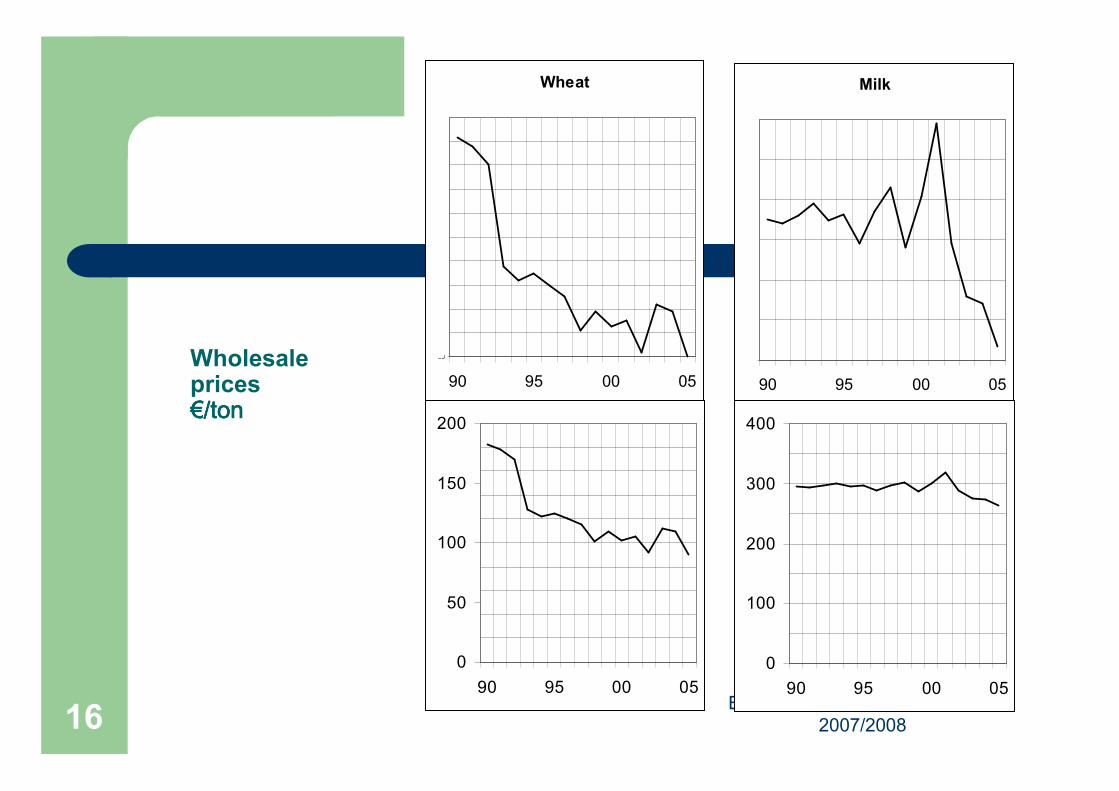
Wholesale prices€€€€/ton/ton/ton/ton

Wheat

90

90 95 00 05

0

50

100

150

200

90 95 00 05

Milk

260

90 95 00 05

0

100

200

300

400

90 95 00 05


2007/200817

Inflation

0

2

4

6

8

0 1 2 3 4 5 6 7 8 9 10

Year

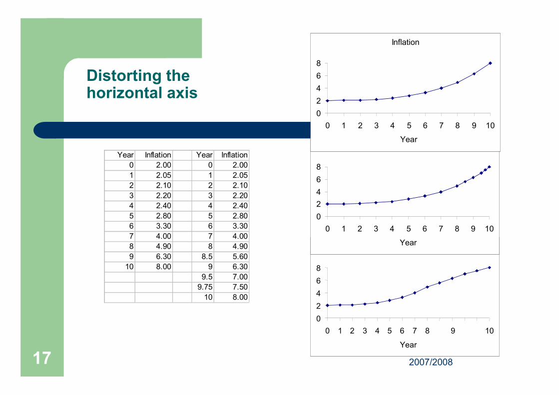
Distorting the horizontal axis

Year Inflation Year Inflation

0 2.00 0 2.00

1 2.05 1 2.05

2 2.10 2 2.10

3 2.20 3 2.20

4 2.40 4 2.40

5 2.80 5 2.80

6 3.30 6 3.30

7 4.00 7 4.00

8 4.90 8 4.90

9 6.30 8.5 5.60

10 8.00 9 6.30

9.5 7.00

9.75 7.50

10 8.00

Inflation

0

2

4

6

8

0 1 2 3 4 5 6 7 8 9 10

Year

Inflation

0

2

4

6

8

0 1 2 3 4 5 6 7 8 9 10

Year


2007/200818

Interest rate of the Central European bank 2.0

2.5

3.0

3.5

4.0

4.5

5.0

08.04.99 16.03.00 31.08.00 30.08.01 05.12.01 01.12.05 03.08.06

0.0

1.0

2.0

3.0

4.0

5.0

01.04.99 31.03.00 31.03.01 31.03.02 31.03.03 30.03.04 30.03.05 30.03.06


2007/200819

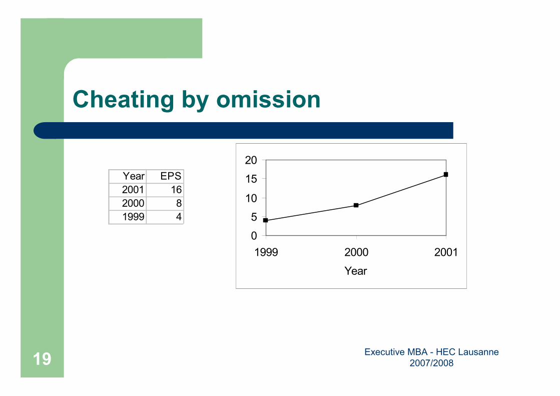
Cheating by omission

Year EPS

2001 16

2000 8

1999 4

0

5

10

15

20

1999 2000 2001

Year


2007/200820

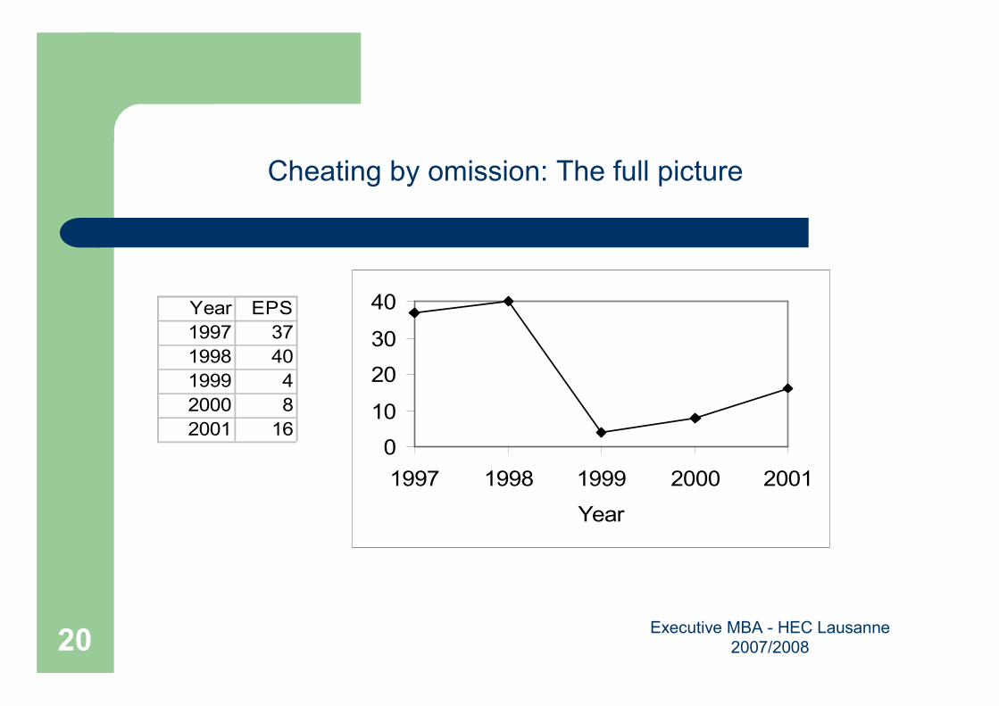
0

10

20

30

40

1997 1998 1999 2000 2001

Year

Year EPS

1997 37

1998 40

1999 4

2000 8

2001 16

Cheating by omission: The full picture


2007/200821

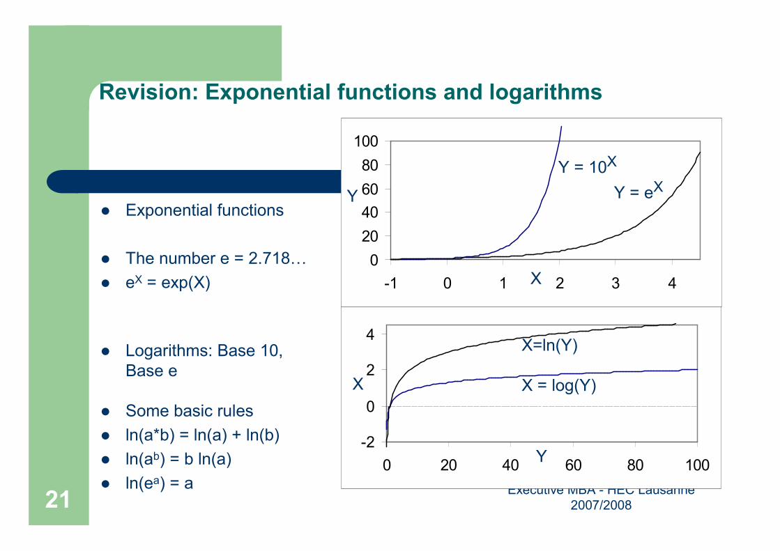
Revision: Exponential functions and logarithms

� Exponential functions

� The number e = 2.718…

� eX = exp(X)

� Logarithms: Base 10,

Base e

� Some basic rules

� ln(a*b) = ln(a) + ln(b)

� ln(ab) = b ln(a)

� ln(ea) = a

-2

0

2

4

0 20 40 60 80 100

0

20

40

60

80

100

-1 0 1 2 3 4

Y = 10X

Y = eX

X=ln(Y)

X = log(Y)

X

Y

X

Y


2007/200822

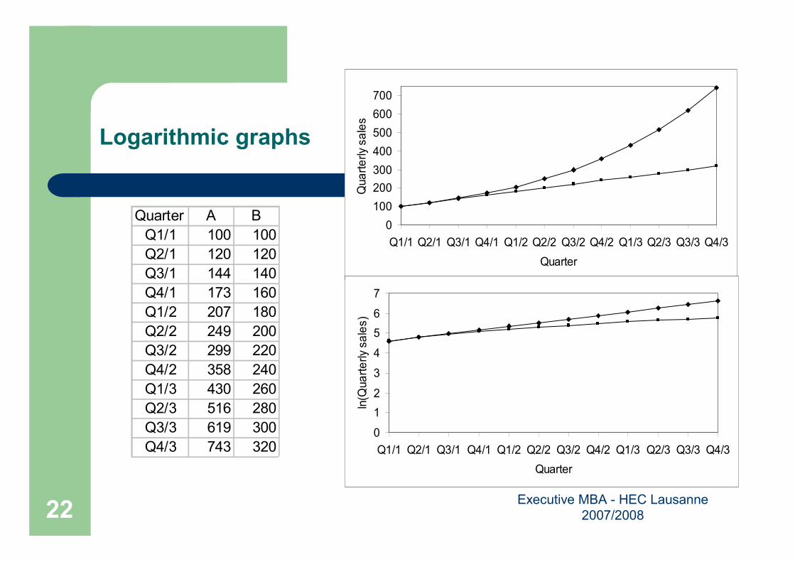
Logarithmic graphs

Quarter A B

Q1/1 100 100

Q2/1 120 120

Q3/1 144 140

Q4/1 173 160

Q1/2 207 180

Q2/2 249 200

Q3/2 299 220

Q4/2 358 240

Q1/3 430 260

Q2/3 516 280

Q3/3 619 300

Q4/3 743 320

0

100

200

300

400

500

600

700

Q1/1 Q2/1 Q3/1 Q4/1 Q1/2 Q2/2 Q3/2 Q4/2 Q1/3 Q2/3 Q3/3 Q4/3

Quarter

Quarterly sales

0

1

2

3

4

5

6

7

Q1/1 Q2/1 Q3/1 Q4/1 Q1/2 Q2/2 Q3/2 Q4/2 Q1/3 Q2/3 Q3/3 Q4/3

Quarter

ln(Quarterly sales)


2007/200823

Visual impression: % change versus actual pattern

-2.00

0.00

2.00

4.00

6.00

8.00

10.00

12.00

14.00

1986 1988 1990 1992 1994 1996

Year

% Change

HIC ABC W&S

0

500

1,000

1,500

2,000

2,500

1986 1988 1990 1992 1994 1996

Year

Actual values

HIC ABC W&S


2007/200824

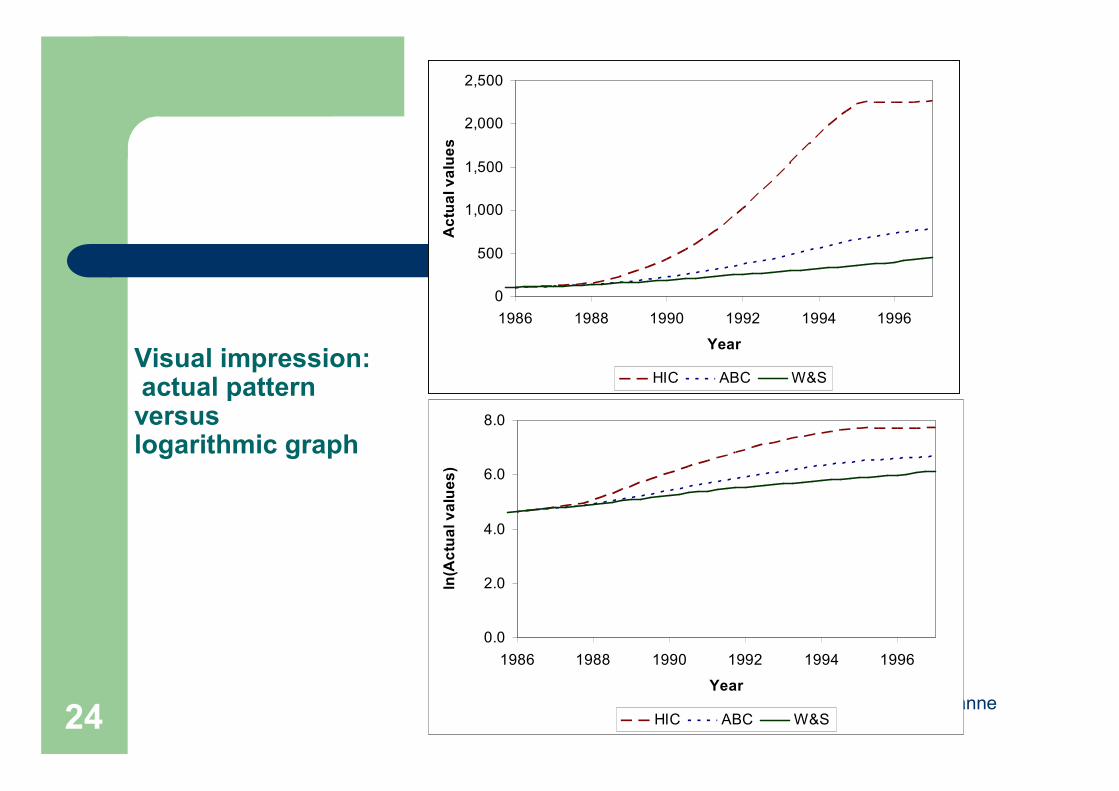
Visual impression: actual pattern versus logarithmic graph

0

500

1,000

1,500

2,000

2,500

1986 1988 1990 1992 1994 1996

Year

Actual values

HIC ABC W&S

0.0

2.0

4.0

6.0

8.0

1986 1988 1990 1992 1994 1996

Year

ln(Actual values)

HIC ABC W&S


2007/200825

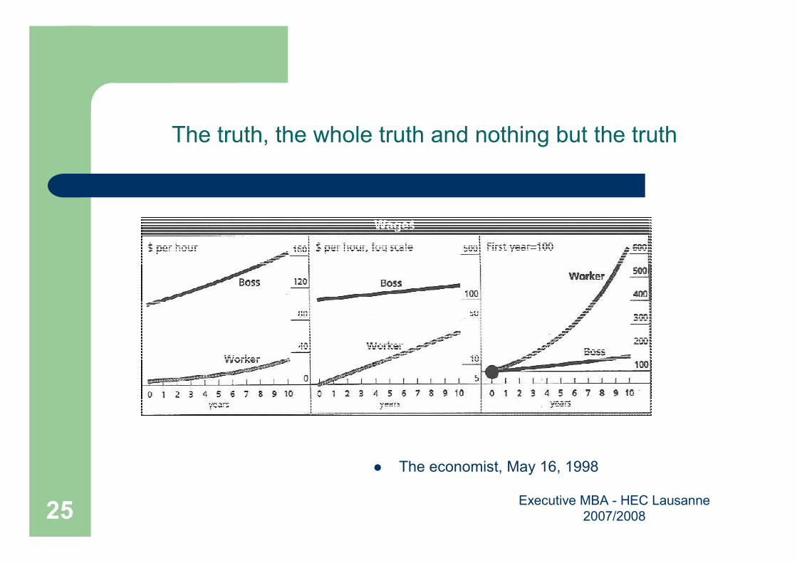
The truth, the whole truth and nothing but the truth

� The economist, May 16, 1998


2007/200826

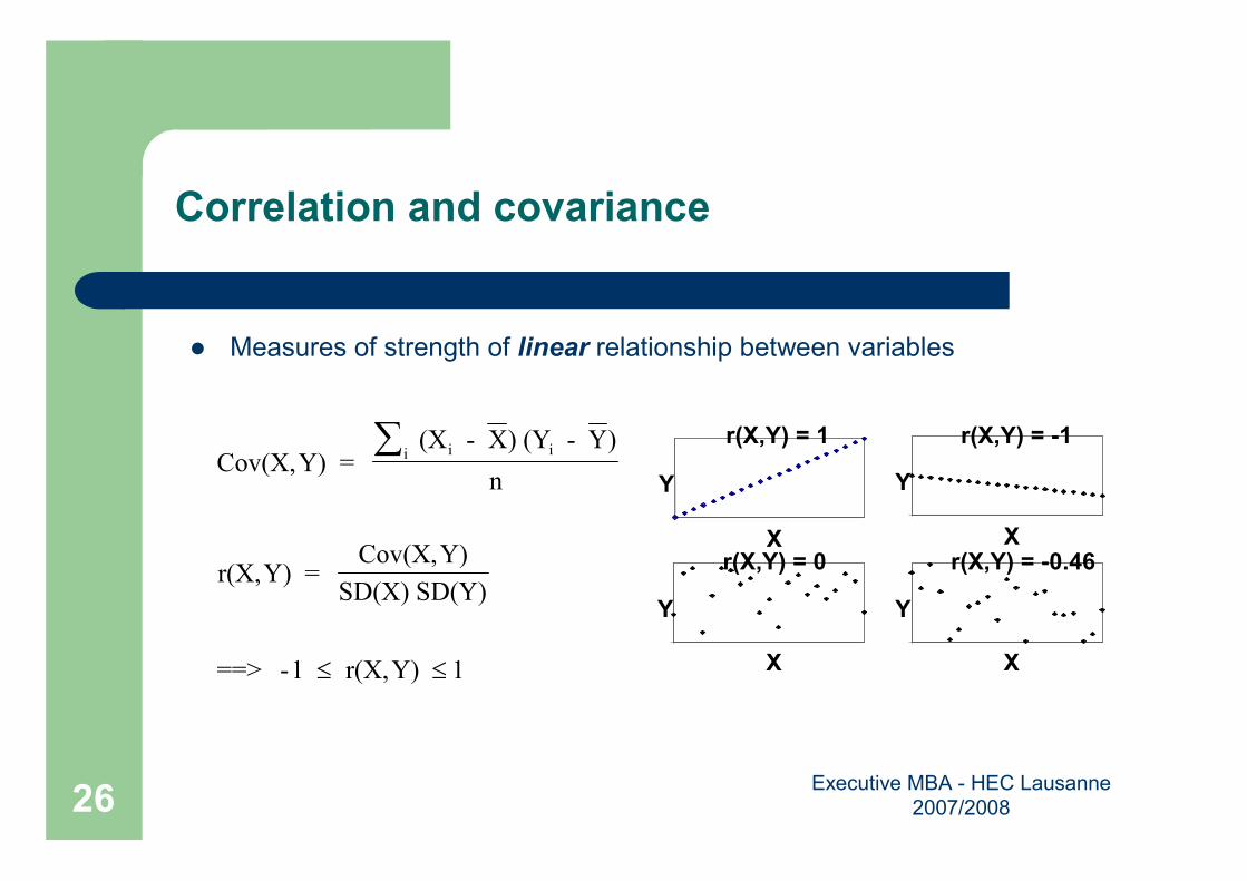
Correlation and covariance

� Measures of strength of linear relationship between variables

r(X,Y) = 1

X

Y

r(X,Y) = -1

X

Y

r(X,Y) = 0

X

Y

r(X,Y) = -0.46

X

Y

Cov(X,Y) = (X - X) (Y - Y)

n

r(X,Y) = Cov(X,Y)

SD(X) SD(Y)

==> -1 r(X,Y)

i ii∑

≤ ≤ 1


2007/200827

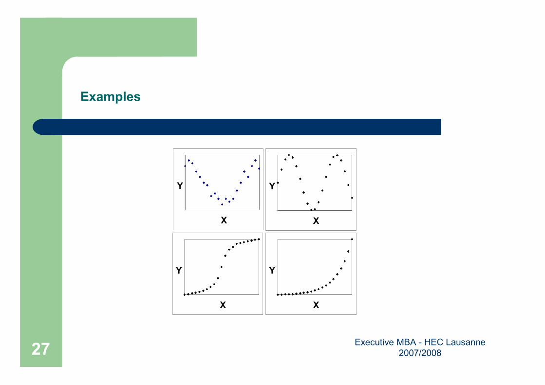
Examples

X

Y

X

Y

X

Y

X

Y


2007/200828

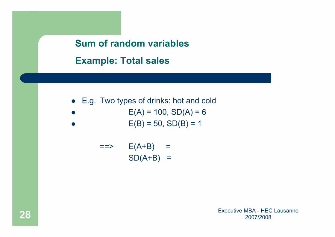
Sum of random variables

Example: Total sales

� E.g. Two types of drinks: hot and cold

� E(A) = 100, SD(A) = 6

� E(B) = 50, SD(B) = 1

==> E(A+B) =

SD(A+B) =


2007/200829

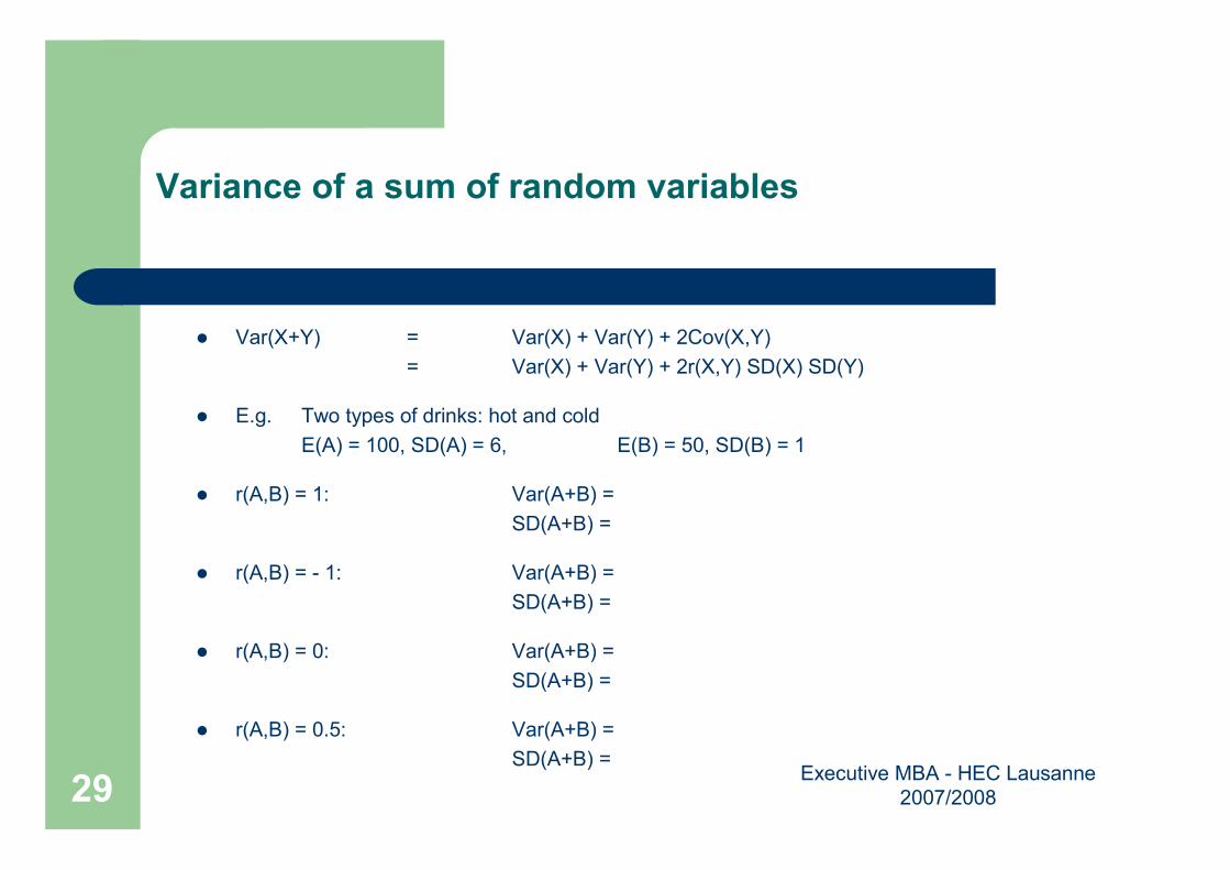
Variance of a sum of random variables

� Var(X+Y) = Var(X) + Var(Y) + 2Cov(X,Y)

= Var(X) + Var(Y) + 2r(X,Y) SD(X) SD(Y)

� E.g. Two types of drinks: hot and cold

E(A) = 100, SD(A) = 6, E(B) = 50, SD(B) = 1

� r(A,B) = 1: Var(A+B) =

SD(A+B) =

� r(A,B) = - 1: Var(A+B) =

SD(A+B) =

� r(A,B) = 0: Var(A+B) =

SD(A+B) =

� r(A,B) = 0.5: Var(A+B) =

SD(A+B) =


2007/200830

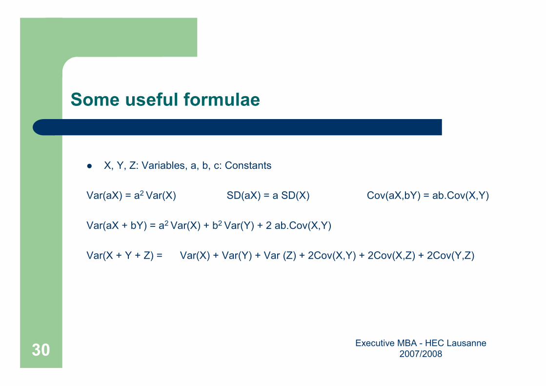
Some useful formulae

� X, Y, Z: Variables, a, b, c: Constants

Var(aX) = a2 Var(X) SD(aX) = a SD(X) Cov(aX,bY) = ab.Cov(X,Y)

Var(aX + bY) = a2 Var(X) + b2 Var(Y) + 2 ab.Cov(X,Y)

Var(X + Y + Z) = Var(X) + Var(Y) + Var (Z) + 2Cov(X,Y) + 2Cov(X,Z) + 2Cov(Y,Z)


2007/200831

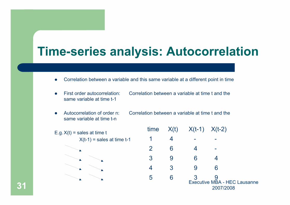
Time-series analysis: Autocorrelation

� Correlation between a variable and this same variable at a different point in time

� First order autocorrelation: Correlation between a variable at time t and the

same variable at time t-1

� Autocorrelation of order n: Correlation between a variable at time t and the

same variable at time t-n

E.g.X(t) = sales at time t

X(t-1) = sales at time t-1

time X(t) X(t-1) X(t-2)

1 4 - -

2 6 4 -

3 9 6 4

4 3 9 6

5 6 3 9


2007/200832

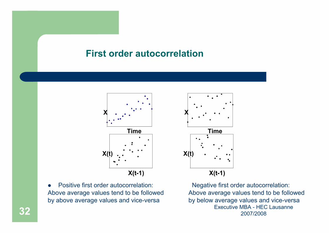
First order autocorrelation

� Positive first order autocorrelation: Negative first order autocorrelation:

Above average values tend to be followed Above average values tend to be followed

by above average values and vice-versa by below average values and vice-versa

Time

X

Time

X

X(t-1)

X(t)

X(t-1)

X(t)


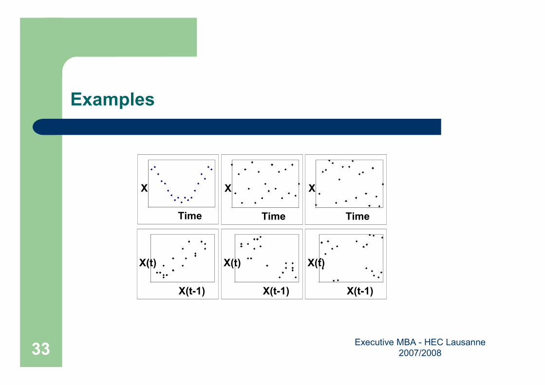
2007/200833

Examples

Time

X

Time

X

X(t-1)

X(t)

X(t-1)

X(t)

Time

X

X(t-1)

X(t)

data, statistics, probability 1 - unil statistics, probability 1.pdf · executive mba -hec lausanne...

Documents