Data Scientist Challenge

by Citi Grouphttps://www.datascientistchallenge.com/

Gautam Kumar (17)

Jaideep Karkhanis(18)

Jayanta Mandi(19)

Sajal Jain(40)

Credit Card Industry

Information rich data

Millions of customers

Transaction data is one good data source

On average approximately 120 annual records are created for each active

customer.

Incredible insights into customer preferences and lifestyle choices.

Sheer size of the data and the processing power required,

Objective

The objective of this challenge is to identify the Top 10 merchants that

customers have not transacted within the past 12 months and are likely to

transact with, in the next 3 months.

Personalize these recommendations at a customer level

Can be used to give customized offers from those merchants to customer,

from whom he is likely to shop.Prime business reason

behind all this analysis

Data Format

Customer # Merchant # Month Category # of transactions

1 1 1 Grocery 3

2 2 1 Dining 2

3 3 1 Grocery 5

4 4 2 Apparel 1

Number of customers: 374328 Number of transaction:63659708

Number of merchants: 9822 Number of merchant categories: 15

Data Summary

No missing data

Data size = 690.5 mb

dim(citi_data)

[1] 18532355 5

range(citi_data$TXN_MTH)

[1] 201309 201408

The15 categories are disjoint sets with merchants

Scoring

If Merchant 1 has been identified correctly for a customer, 10 points are added

to the score. Correctly identifying Merchant 2 adds 9 points, and so on.

Code to be executed on a High Performance Machine with 96 GB RAM.

Algorithm should run within 12 hours in terms of execution time.

Category of Problem

It was a collaborative filtering problem, where people can be recommended about

items with similar taste have bought before.

Approaches Tried

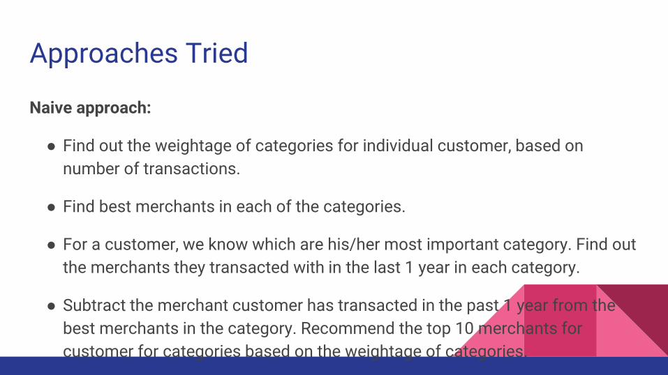
Naive approach:

● Find out the weightage of categories for individual customer, based on

number of transactions.

● Find best merchants in each of the categories.

● For a customer, we know which are his/her most important category. Find out

the merchants they transacted with in the last 1 year in each category.

● Subtract the merchant customer has transacted in the past 1 year from the

best merchants in the category. Recommend the top 10 merchants for

customer for categories based on the weightage of categories.

Approaches Tried (Continued...)

● Data seems to be time (quarter) independent.

● Additional weightage to the 1st quarter as we need to predict for next 1st

quarter.

● Detailed time series analysis doesn’t seem to be appropriate. (¼th of the total

time duration we need to predict).

● Cyclicity in terms of annual transactions.

Approaches Tried (Continued...)

Matrix factorization based collaborative filtering:

● Create a matrix which is a Customer x Merchant Matrix. Each element

represents the number of transactions a customer has done with the specific

matrix. Since normal matrix of size 3,75,000 x 10,000 was not possible, so we

create a sparse matrix.

● We factorized the sparse matrix doing SVD using “Irlba” package.

● We did SVD using 10,20,30,50,75,100,125,150,200 rank approximations

● We reconstruct one row of the original at a time by doing Ui X Eii X Vi

SVD based method explained

The reduced orthogonal dimensions resulting from SVD are less noisy than the original

data and capture the latent associations

Reducing the dimensionality of the customer-merchant space, we can increase density of

the matrix and thereby generate predictions

SVD provides the best lower rank approximations of the original matrix R, in terms of

Frobenius norm

The reconstructed matrix Rk = Uk.Sk.Vk’ minimizes the Frobenius norm i.e. || R- Rk ||

over all rank-k matrices

Even though the Rk matrix is dense, its special structure allows us to use sparse SVD

algorithms (e.g. Lanczos) whose complexity is almost linear to the number of nonzeros

in the original matrix R.

SVD based method explained

We use SVD in recommender systems to perform 2 different tasks:-

First, we use SVD to capture the latent relationships between customers and merchants that

allow us to compute the predicted likeliness of a certain merchant by a customer.

Second, we use SVD to produce a low-dimensional representation of the original customer-

merchant space and then compute neighborhood in the reduced space. We then use that to

generate a list of top-N product recommendations for customers.

SVD based method explained

The optimal choice of the value ‘k’ is critical to high quality prediction

generation.

We are interested in a value of k that is large enough to capture all the important

structures in the matrix yet small enough to avoid overfitting errors.

For an m x n matrix the SVD decomposition requires a time in the order of

O((m+n)^3)

In terms of storage SVD is efficient. We need to store just two reduced

customer and merchant matrices of size m x k and k x n respectively, a total

of O(m+n), since k is constant.

Singular Value decomposition

Singular value decomposition

K-Rank Approximation

Approaches Tried (Continued...)

● Reconstruction of a row, representation of behaviour which is expected

behaviour for a particular customer. This means the row we get after re

construction gives an idea of, which merchants the customer would have

bought normally.

● So we take the difference of this reconstructed row from the original given

row and see that, which are the entries in the row which changed from zero to

nonzero.

● These elements will give the merchants from whom the customer are

expected to buy. So we select the 10 merchants and recommend for that

customer.

Plot of 1st 100 eigen values

Plot of 2nd to 200th eigen values

Log-plot of 1st 1500 Merchants by Transactions

• The Implicitly Restarted Lanczos bidiagonalization algorithm (IRLBA) of Jim Baglama and Lothar Reichel is a state of the art method for computing a few singular vectors and corresponding singular values of huge matrices.

• With it, computation of partial SVDs and principal component analyses of very large scale data is very time and space -efficient. The package works well with sparse matrices.

What is IRLBA?

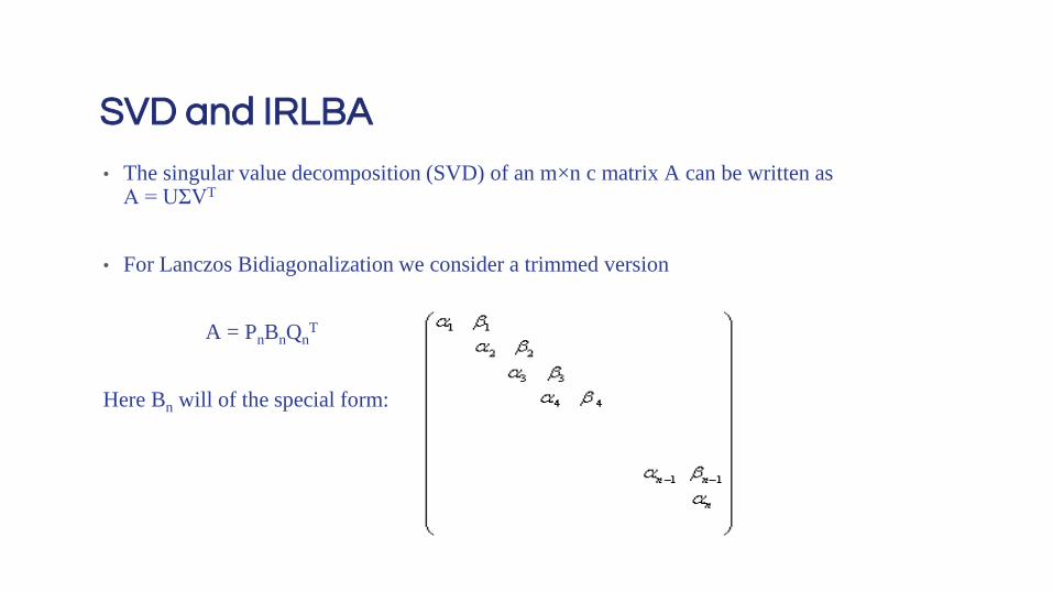
• The singular value decomposition (SVD) of an m×n c matrix A can be written as A = UΣVT

• For Lanczos Bidiagonalization we consider a trimmed version

A = PnBnQnT

Here Bn will of the special form:

SVD and IRLBA

• Expressions can be written in vector form by equating the jth column

• Aqj = βj-1 pj−1 + αjpj,

• ATpj = αjqj + βjqj+1.

• From This we can obtain the recursive relation:

• αjpj = Aqj −βj−1pj−1

• βjqj+1 = ATpj −αjqj

Bidiagonalization Algorithm

••

Partial Lanczos Bidiagonalization:Algorithm

Verifying for the algorithm

Sampling small chunk and then ensembling the data

For verifying the algorithm, took first 9 month data

Predicted for next 3 months

Compared with the data which we have.

Random samples of 10,000 customers were taken for each trial.

Keep taking samples and average if value already exists.

•

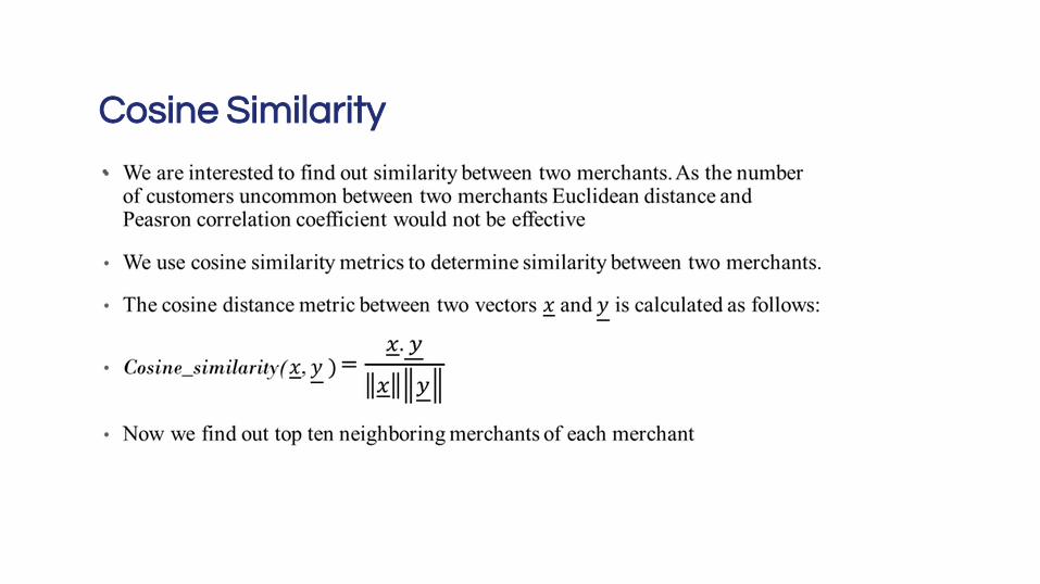
Cosine Similarity

•

Generating Score function for each customer

References

“Application of Dimensionality Reduction in Recommender System - A Case Study” Badrul M. Sarwar,

George Karypis, Joseph A. Konstan, John T. Riedl Department of Computer Science and Engineering,

University of Minnesota

“Topics in Data Analytics: Collaborative Filtering, Finding Similar Items in Very High Dimension,

Sentiment Analysis”

Debapriyo Majumdar, Indian Statistical Institute Kolkata

http://www.math.kent.edu/~reichel/publications/blklbd.pdf

http://qubit-ulm.com/wp-content/uploads/2012/04/Lanczos_Algebra.pdf