data replication and fault tolerance in...

UNIVERSITY OF CALIFORNIA,IRVINE

Data Replication and Fault Tolerance in AsterixDB

THESIS

submitted in partial satisfaction of the requirementsfor the degree of

MASTER OF SCIENCE

in Computer Science

by

Murtadha Al Hubail

Thesis Committee:Professor Michael J. Carey, Chair

Professor Chen LiAssistant Professor Ardalan Amiri Sani

2016

DEDICATION

To my parentsyour prayers will always guide my path in this life.

To my wife Sukainah and my daughter MariaI hope that someday I can repay you for all the sacrifices you made during this journey.

To my brothers and sistersfor their continuous prayers, support, and encouragement.

To my dearest friendAbdullah Alamoudi

for his support and encouragement throughout this journey.

ii

TABLE OF CONTENTS

Page

LIST OF FIGURES v

LIST OF TABLES vi

ACKNOWLEDGMENTS vii

ABSTRACT OF THE THESIS viii

1 Introduction 1

2 Related Work 32.1 Replication in Database Systems . . . . . . . . . . . . . . . . . . . . . . . . 3

2.1.1 Consistency Models . . . . . . . . . . . . . . . . . . . . . . . . . . . . 32.1.2 Centralized Database Systems . . . . . . . . . . . . . . . . . . . . . . 42.1.3 Parallel Database Systems . . . . . . . . . . . . . . . . . . . . . . . . 5

2.2 Replication in Big Data Systems . . . . . . . . . . . . . . . . . . . . . . . . . 82.2.1 The CAP Theorem and Consistency Models . . . . . . . . . . . . . . 82.2.2 Google Bigtable and Apache HBase . . . . . . . . . . . . . . . . . . . 92.2.3 Amazon Dynamo . . . . . . . . . . . . . . . . . . . . . . . . . . . . . 92.2.4 Apache Cassandra . . . . . . . . . . . . . . . . . . . . . . . . . . . . 102.2.5 Yahoo PNUTS . . . . . . . . . . . . . . . . . . . . . . . . . . . . . . 102.2.6 Spinnaker . . . . . . . . . . . . . . . . . . . . . . . . . . . . . . . . . 11

3 AsterixDB Background 123.1 AsterixDB Architecture . . . . . . . . . . . . . . . . . . . . . . . . . . . . . 123.2 AsterixDB Data Model . . . . . . . . . . . . . . . . . . . . . . . . . . . . . . 143.3 AsterixDB Query Language . . . . . . . . . . . . . . . . . . . . . . . . . . . 143.4 AsterixDB Storage and Transaction Model . . . . . . . . . . . . . . . . . . . 15

4 AsterixDB Data Replication and Fault Tolerance 184.1 Basic Design . . . . . . . . . . . . . . . . . . . . . . . . . . . . . . . . . . . . 18

4.1.1 Data Consistency . . . . . . . . . . . . . . . . . . . . . . . . . . . . . 194.1.2 Replication Factor . . . . . . . . . . . . . . . . . . . . . . . . . . . . 194.1.3 Primary and Remote Replicas . . . . . . . . . . . . . . . . . . . . . . 204.1.4 Replica Placement and Remote Primary Replicas . . . . . . . . . . . 20

iii

4.2 Implementation of Replication . . . . . . . . . . . . . . . . . . . . . . . . . . 214.2.1 Job Replication Protocol . . . . . . . . . . . . . . . . . . . . . . . . . 214.2.2 LSM Disk Component Replication Protocol . . . . . . . . . . . . . . 234.2.3 Replica Checkpointing Coordination . . . . . . . . . . . . . . . . . . 27

4.3 Implementation of Fault Tolerance . . . . . . . . . . . . . . . . . . . . . . . 294.3.1 Node Failover . . . . . . . . . . . . . . . . . . . . . . . . . . . . . . . 294.3.2 Node Failback . . . . . . . . . . . . . . . . . . . . . . . . . . . . . . . 31

4.4 Design Discussion . . . . . . . . . . . . . . . . . . . . . . . . . . . . . . . . . 364.4.1 Data Inconsistency Window . . . . . . . . . . . . . . . . . . . . . . . 364.4.2 Temporary Remote Replica Inconsistency . . . . . . . . . . . . . . . 364.4.3 Node Failover Time Estimation . . . . . . . . . . . . . . . . . . . . . 37

5 Initial Performance Evaluation 385.1 Experimental Setup . . . . . . . . . . . . . . . . . . . . . . . . . . . . . . . . 385.2 Results and Analysis . . . . . . . . . . . . . . . . . . . . . . . . . . . . . . . 40

5.2.1 Bulk load Time . . . . . . . . . . . . . . . . . . . . . . . . . . . . . . 405.2.2 Ingestion Time . . . . . . . . . . . . . . . . . . . . . . . . . . . . . . 415.2.3 Query Response Time . . . . . . . . . . . . . . . . . . . . . . . . . . 435.2.4 Failover and Failback Time . . . . . . . . . . . . . . . . . . . . . . . 44

6 Conclusion and Future Work 496.1 Conclusion . . . . . . . . . . . . . . . . . . . . . . . . . . . . . . . . . . . . . 496.2 Future Work . . . . . . . . . . . . . . . . . . . . . . . . . . . . . . . . . . . . 50

6.2.1 Delta Recovery During Failback . . . . . . . . . . . . . . . . . . . . . 506.2.2 Hot Standby Remote Replica . . . . . . . . . . . . . . . . . . . . . . 506.2.3 Cluster Controller Fault Tolerance . . . . . . . . . . . . . . . . . . . . 516.2.4 AsterixDB Cluster Scaling . . . . . . . . . . . . . . . . . . . . . . . . 51

Bibliography 52

iv

LIST OF FIGURES

Page

2.1 Data placement with Tandem’s mirrored disks scheme . . . . . . . . . . . . . 62.2 Data placement in interleaved declustering with group size = 3 . . . . . . . . 72.3 Data placement in chained declustering with relation-cluster size = 6 . . . . 8

3.1 AsterixDB’s architecture . . . . . . . . . . . . . . . . . . . . . . . . . . . . . 133.2 Log record format . . . . . . . . . . . . . . . . . . . . . . . . . . . . . . . . . 16

4.1 AsterixDB cluster with 3 nodes . . . . . . . . . . . . . . . . . . . . . . . . . 194.2 Primary and remote replicas with replication factor = 3 . . . . . . . . . . . . 204.3 Job replication protocol . . . . . . . . . . . . . . . . . . . . . . . . . . . . . 224.4 Additional log fields . . . . . . . . . . . . . . . . . . . . . . . . . . . . . . . . 224.5 Flushed LSM component replication . . . . . . . . . . . . . . . . . . . . . . 254.6 Lagging replica index . . . . . . . . . . . . . . . . . . . . . . . . . . . . . . . 284.7 Cluster state before any node failures with replication factor = 3 . . . . . . . 304.8 Data partition failover logic . . . . . . . . . . . . . . . . . . . . . . . . . . . 314.9 Cluster state after Node 1 partitions failover to Node 2 and Node 3 with

replication factor = 3 . . . . . . . . . . . . . . . . . . . . . . . . . . . . . . . 324.10 Node failback initiation logic . . . . . . . . . . . . . . . . . . . . . . . . . . . 334.11 Cluster state before Node 1 failback with replication factor = 3 . . . . . . . 344.12 Node failback completion logic . . . . . . . . . . . . . . . . . . . . . . . . . . 344.13 Cluster state after Node 1 failback with replication factor = 3 . . . . . . . . 35

5.1 Bulk load time with different replication factors . . . . . . . . . . . . . . . . 415.2 Ingestion time with different replication factors . . . . . . . . . . . . . . . . 425.3 Query response time (dataset size = 15 million records) during ingestion . . 445.4 Failover time (replication factor = 3, no checkpointing) . . . . . . . . . . . . 455.5 Ingestion time with different memory component sizes (replication factor = 3) 465.6 Checkpoint interval impact on failover time (dataset size = 20 million records,

replication factor = 3) . . . . . . . . . . . . . . . . . . . . . . . . . . . . . . 475.7 Failback time (replication factor = 3) . . . . . . . . . . . . . . . . . . . . . . 47

v

LIST OF TABLES

Page

5.1 Experiments’ datasets . . . . . . . . . . . . . . . . . . . . . . . . . . . . . . 40

vi

ACKNOWLEDGMENTS

I would like to thank my advisor Prof. Michael Carey for being a friend with his studentsbefore a mentor. His dedication, knowledge, humility, and sense of humor is a hard combi-nation to come by. I consider myself very lucky to have had the chance to work with him.Words cannot express my gratitude to Prof. Carey and I will always be indebted to him.

I would like to thank Abdullah Alamoudi for his invaluable support throughout this project.I would like to also thank Ian Maxon for his continuous support and reviewing my code. Iwould like to thank everyone in AsterixDB’s team for their support and contribution to theproject.

I would like to thank my thesis committee members Prof. Chen Li and Assistant Prof.Ardalan Amiri Sani for reviewing my thesis.

I would like to thank Saudi Aramco for sponsoring my scholarship.

This thesis was supported in part by NSF grants (CNS-1059436 and CNS-1305430).

vii

ABSTRACT OF THE THESIS

Data Replication and Fault Tolerance in AsterixDB

By

Murtadha Al Hubail

Master of Science in Computer Science

University of California, Irvine, 2016

Professor Michael J. Carey, Chair

AsterixDB is a Big Data Management System (BDMS) that is designed to run on large

clusters of commodity hardware. In such clusters however, hardware failures are inevitable.

To tolerate these failures, data replication strategies are used. Over the years, many data

replication strategies have been proposed with different trade-offs between data consistency,

throughput, and recovery time.

In this thesis, we describe our new data replication protocol for AsterixDB that guar-

antees data consistency and exploits the properties of Log-Structured Merge-trees to achieve

efficient data replication and controllable recovery time. We explain in detail the data

replication protocol design and implementation. We then explain how fault tolerance is im-

plemented on top of the data replication protocol. We further provide an initial evaluation

of the data replication protocol and show how three replicas of the data can be maintained

with only 6% to 14% increase in ingestion time for certain ingestion workloads. We also

show how a recovery time as low as one second can be achieved.

viii

Chapter 1

Introduction

In this era of Big Data and cloud computing, many applications have high scalability and

availability requirements that cannot be handled by traditional centralized data management

systems. To meet such high-scalability requirements in a cost-effective manner, data is

usually partitioned across commodity hardware computing clusters [18, 16, 12]. As clusters

grow larger and larger however, hardware failures become unavoidable. To tolerate hardware

failures, data-replication strategies are used.

When designing a data-replication strategy, many decisions have to be made. These deci-

sions include, but are not limited to, what consistency constraints should be guaranteed,

what is an acceptable recovery time in case of failures, where to place different replicas,

how to load balance workloads across replicas, and how to reach consensus between replicas

in case of failures. Looking at these decisions, it can be easily concluded that designing a

data-replication protocol is a complex task and requires a careful design as well as imple-

mentation. One thing for certain is that data replication always comes at cost. This cost

results from the extra computational overhead, memory usage, and networking required to

perform replication.

1

Over the years, many data replication strategies have been proposed [21, 31, 25]. Some of

them focus on providing high availability and low recovery time at the expense of throughput.

Others try to minimize the throughput penalty at the cost of data consistency. For this thesis,

we have implemented an efficient data-replication protocol for AsterixDB that guarantees

data consistency, provides a controllable recovery time, yet has a low impact on throughput

as well as on the computational resources required for replication. This goal was achieved

by exploiting the properties of the underlying Log-Structured Merge-tree (LSM-tree) [33]

storage in AsterixDB.

In this thesis, we start by discussing related work in Chapter 2 and provide background infor-

mation about AsterixDB in Chapter 3. Chapter 4 describes the design and implementation

of the new AsterixDB data replication protocol and how fault tolerance was implemented

on top of the replication protocol. We present an intial performance evaluation in Chapter

5. In Chapter 6, we conclude the thesis.

2

Chapter 2

Related Work

2.1 Replication in Database Systems

In this section, we start by describing the consistency models used in database system

replication. After that, we review some of the proposed schemes in both centralized –

i.e., unpartitioned – databases as well as parallel database systems.

2.1.1 Consistency Models

Replication strategies in database systems can be categorized, based on consistency models,

into two major categories [22]: 2-safe (synchronous) and 1-safe (asynchronous) algorithms.

In 2-safe algorithms, the primary and backup are kept in-sync all the time. Transactions

are not committed on the primary site until all of their updates have been received and

acknowledged by the backup site. Thus, 2-safe algorithms guarantee the survival of all

committed transactions in case of failures. However, since updates are performed at both

sites at the same time, transaction latency increases by at least one round trip for the

3

coordination between the primary and backup sites. For this reason, 1-safe algorithms have

been proposed. In 1-safe algorithms, transactions are committed on the primary first and

their updates are asynchronously sent to the backup. While 1-safe algorithms provide better

response times than 2-safe, if a crash happens on the primary site before a committed

transaction’s updates are received by the backup, the effects of the transaction are lost.

Therefore, 1-safe algorithms are better suited for applications that favor higher throughput

and can afford to lose a few committed transactions, whereas 2-safe algorithms are needed

for applications that require survival of all committed transactions.

2.1.2 Centralized Database Systems

Most of the replication schemes in centralized database systems rely on the fact that a

committed transaction’s updates are recorded in the database transaction log. Therefore,

replication is done by sending transaction log records to the backup sites. Below, we describe

how replication is implemented in the popular database system MySQL.

MySQL

The default replication scheme in MySQL v5.7 [4] is asynchronous (1-safe). All changes to

the database are recorded in the master’s (primary site’s) binary log files. Slaves (backups)

connect to the master and continuously request a copy of the latest logs. After that, each

slave replays the committed transactions in the same order they appear in the received

logs, therefore reaching the same eventual consistent state as the master. For this to work

correctly, it is required that the master and slaves have the information about the log files

and their positions synchronized.

Since MySQL v5.7, a new type of replication scheme, which is called “semisynchronous”,

4

is supported as well. Semisynchronous replication tries to balance between the data con-

sistency of synchronous replication and the better throughput of asynchronous replication.

In MySQL’s semisynchronous scheme, a committed transaction on the master waits until at

least one of the slaves has acknowledged that it has received, though not necessarily replayed,

the transaction updates. To avoid making the master wait indefinitely, after a timeout pe-

riod passes, the master switches to asynchronous replication. Eventually, when at least one

of the slaves catches up, the master switches back to semisynchronous mode.

2.1.3 Parallel Database Systems

In parallel database systems [18], data is partitioned across multiple processors (nodes) and

disks using a partitioning technique. The underlying hardware for these systems is often a

proprietary cluster. Replication in such systems is a more complex task than in centralized

database systems. Below, we describe some of the proposed replication schemes which can

tolerate the failure of a single node or disk.

Mirrored Disks

In the mirrored disks [10] replication scheme, which was used in Tandem’s NonStop SQL

system [7], each disk is completely mirrored to another disk. Furthermore, each disk is

connected to two I/O controllers, and two nodes are connected to each I/O controller. Thus,

there is a completely independent path from each mirror node to each disk. To scale, a

relation R can be partitioned (declustered) across a number of nodes and disks. Figure 2.1

shows Tandem’s mirrored disks data placement for a relation R that is two-way partitioned

and thus mirrored across two nodes and four disks. In the figure, Ri represents partition i

of the relation R, while ri represents the mirror of that partition. In this scheme, partition

read requests can be served by either the disk containing the original copy or by its mirror.

5

Figure 2.1: Data placement with Tandem’s mirrored disks scheme

However, write requests must be synchronized across a disk and its mirror. As Figure 2.1

shows, if a single disk fails, its data partition can still be read and written from its mirror.

Similarly, if a node fails, the other node still has access to all disks.

Interleaved Declustering

In this replication scheme, which is implemented in Teradata’s parallel database system [6],

nodes are divided into groups of size N. Each node in the group holds the primary copy of

a data partition (fragment). A backup copy for each fragment is created by subdividing the

primary fragment into (N-1) subfragments, and each subfragment is stored in the remaining

nodes in the group. Figure 2.2 shows the data placement under the interleaved declustering

scheme for a cluster consisting of 6 nodes and a group size of N = 3. In the figure, Ri

represents the primary fragment i, whereas ri.j represents each of the subfragments j of

fragment i.

In case a node fails, its primary fragment is served from its subfragments in the other nodes.

Moreover, interleaved declustering provides better load balancing in case of a node failure

than mirrored disks since the load of the failed node will be distributed among the remaining

N-1 nodes in the group rather than overloading one node. If a second node in the same group

6

Group 0 Group 1Node 0 1 2 3 4 5

Primary Copy R0 R1 R2 R3 R4 R5Backup Copy r0.0 r0.1 r3.0 r3.1

r1.1 r1.0 r4.1 r4.0r2.0 r2.1 r5.0 r5.1

Figure 2.2: Data placement in interleaved declustering with group size = 3

fails, all the data in that group becomes unavailable. It is worth noting that the probability

of losing a group’s data increases proportionally as the size of the group increases [25].

Chained Declustering

In chained declustering [24], nodes are divided into groups called “relation-clusters”, and

each relation-cluster may also be divided into smaller groups called “chain-clusters”. Similar

to interleaved declustering, two copies (primary and backup) of each data fragment are

maintained. Unlike interleaved declustering, the backup copy is not subfragmented. The

placement of each primary fragment and its backup is done as follows: if there are N nodes,

ordered from 0 to N-1, in a relation-cluster, the ith primary fragment is placed in the node

[i + C(R) mod N], whereas its backup is placed in [i + 1 + C(R) mod N], where the

function C(R) allows the assignment of the first fragment to any node. Figure 2.3 shows the

primary and backup placement using the chained declustering scheme on a relation-cluster

consisting of 6 nodes. In the figure, Ri represents the primary copy of the fragment, whereas

ri represents its backup copy.

In case a node fails, its primary fragment is served from the node that has its backup.

Moreover, chained declustering can support even load balancing for read queries after a

node failure by carefully redistributing the workload between primary and backup copies

[24]. Furthermore, unlike interleaved declustering, if more than one node fails within the

same relation-cluster, all data is still available as long as two failing nodes are not logically

7

Node 0 1 2 3 4 5Primary Copy R0 R1 R2 R3 R4 R5Backup Copy r5 r0 r1 r2 r3 r4

Figure 2.3: Data placement in chained declustering with relation-cluster size = 6

adjacent in the relation-cluster. [25] provides a detailed performance study for these three

replication schemes for parallel database systems.

2.2 Replication in Big Data Systems

In recent years, a number of applications have emerged that have high scalability and avail-

ability requirements that could not be handled by traditional database systems. This trend

led to the development of so-called NoSQL datastores [32]. To meet the high scalability

requirements in these datastores in a cost-effective way, data is partitioned on large com-

modity clusters. In such clusters, however, hardware failures become inevitable. To tolerate

these failures and satisfy the high-availability requirement, multiple replicas of each data

partition are maintained. This design led to new challenges, such as reaching consensuses

between replicas during failures, in designing replication schemes. In this section, we start by

describing the famous CAP theorem and the data consistency models in NoSQL datastores.

After that, we describe how high-availability is achieved in some NoSQL datastores.

2.2.1 The CAP Theorem and Consistency Models

In his CAP theorem [13], Brewer states that in distributed systems, only two out of {Consistency,

Availability, and Partition tolerance} can be achieved. Since availability is essential in most

of today’s applications, systems designers have to decide between consistency and network

partitioning tolerance. Systems that choose to implement consistency are said to employ

8

a strong consistency model. In this model, all replicas appear to applications to be in

a consistent state. Some applications, with extreme high availability requirements, prefer

network partitioning tolerance over consistency. Such applications are said to employ an

eventual consistency model [36]. In such systems, when network partitioning happens,

write conflicts may happen and replicas may diverge. Therefore, applications that choose

eventual consistency need to implement conflict resolution protocols.

2.2.2 Google Bigtable and Apache HBase

One way to implement a datastore with high availability and strong consistency is to build

it on top of a distributed file system which supports replication. Google’s Bigtable [14] is

an example of such datastore. It uses Google’s File System (GFS) [20] to store its data as

well as its logs. Its data model consists of tables that are range-partitioned on a primary

key. Apache’s HBase [2] is an open source datastore which is based on the Bigtable design

and built on top of the Hadoop Distributed File System [35]. It is worth noting that using a

distributed file system is not ideal for transactional systems. The reason for this is that every

log page, when forced to disk, needs to go through the distributed file system replication

protocol. Bigtable designers highlighted the drawbacks of using GFS, which has a single

master node, as the underlying storage for Bigtable in [30].

2.2.3 Amazon Dynamo

Amazon’s Dynamo [17] is a highly-available, highly-scalable key-value store with eventual

consistency. Dynamo uses consistent hashing [27] for key space partitioning to achieve in-

cremental scalability. A node is responsible for any key that falls within its range as well

as for replicating its data to other replicas. The result of each modification operation on

a key is considered as a new and immutable version. Eventually, newer versions subsume

9

previous version(s) in all replicas. However, in the presence of failures, multiple conflicting

versions of a key may exist. To resolve these conflicts, Dynamo utilizes vector clocks [19, 29]

with reconciliation during reads (i.e., the client is presented with all conflicting versions and

has to resolve conflicts “manually”). For detecting replicas’ splits and joins, a gossip-based

protocol is used to propagate membership changes between replicas.

2.2.4 Apache Cassandra

Originally designed at Facebook, Apache Cassandra [1] is an open source distributed database

system. It borrows its high-availability design from Amazon’s Dynamo system but takes its

data model from Google’s Bigtable system. For key-based partitioning, Cassandra supports

Random Partitioning as well as Order-Preserving Partitioning. Cassandra has a configurable

consistency model. It supports strong consistency, which is encouraged for use within a data

center, as well as eventual consistency, which is meant to be used across data centers.

2.2.5 Yahoo PNUTS

Yahoo’s PNUTS [15] system is a scalable datastore that has a similar data model as Google’s

Bigtable. In addition, each record (key) has a master replica that is determined by a parti-

tioning algorithm. Replication is done using a reliable publish/subscribe service called the

Yahoo Message Broker (YMB). Transactions are not committed on the master replica un-

til they are sent to YMB. By exploiting the messaging order properties of YMB, PNUTS

provides a timeline consistency [15] model. Under timeline consistency, a record’s updates

are guaranteed to be applied in the same order, but not necessarily at the same time, on

all replicas. Therefore, unlike eventual consistency, no write conflicts between replicas may

occur. For reading a record, PNUTS supports a range of APIs that include Read-any, where

a potentially stale value may be returned; Read-critical(required version), where a newer

10

version than required version is returned; and Read-latest, where the latest version of the

record is returned.

2.2.6 Spinnaker

Spinnaker [34] is an experimental, scalable, consistent, highly-available datastore from IBM

Research. It has a data model similar to Google’s Bigtable and uses key-based range par-

titioning. It uses the previously described chained declustering scheme; the relation-cluster

groups, called “cohorts” in Spinnaker, consist of each range partition and its replicas. Ini-

tially, each cohort has an elected leader and two followers. Its replication protocol works as

follows: when a client submits a write transaction t, its logs are forced to disk on the leader

but it is not yet committed. After that, t is proposed to the followers. When at least one

follower has forced t ’s logs to disk and sent an acknowledgment to the leader, the leader

commits t and returns to the client. At the same time, the leader sends an asynchronous

commit message to the followers to commit t. For read transactions, Spinnaker supports

strong consistency, where reads are always routed to the leader, as well as timeline consis-

tency, where reads may be routed to followers and a potentially stale value may be returned.

When a cohort leader fails, a leader election protocol is followed, which uses Paxos [28] that

is implemented in ZooKeeper [26] to guarantee that a consensus will be reached within the

nodes of the cohort. A cohort’s data continues to be available and strongly consistent as

long as two nodes are up in the cohort.

11

Chapter 3

AsterixDB Background

AsterixDB is a Big Data Management System (BDMS) with a set of unique features that

distinguishes it from other Big Data platforms. AsterixDB’s features make it particularly

well-suited for applications such as social data storage and analysis, data warehousing, and

many other Big Data applications.

AsterixDB runs on top of Hyracks, which is an open source platform designed to run data-

intensive computations on large clusters [11]. A detailed description of AsterixDB can be

found in [8]. In this chapter, we will start by giving a brief description of AsterixDB’s

architecture, data model, and query language. After that, we will zoom in AsterixDB’s

storage and transaction model, which the new replication protocol was built on top of.

3.1 AsterixDB Architecture

Figure 3.1 provides a high-level overview of AsterixDB and its basic logical architecture.

Data enters the system through loading, continuous ingestion feeds [23], and/or insertion

queries. Data is accessed via queries and the return (synchronously or asynchronously)

12

Figure 3.1: AsterixDB’s architecture

of their results. AsterixDB aims to support a wide range of query types, including large

queries (like current Big Data query platforms), short queries (like current key-value stores),

as well as everything in between (like traditional parallel databases). The Cluster Controller

in Figure 3.1 is the logical entry point for user requests; the Node Controllers (NCs) and

Metadata (MD) Node Controller provide access to AsterixDB’s metadata and the aggregate

processing power of the underlying shared-nothing cluster. AsterixDB has a typical layered

DBMS-like architecture that operates on nodes of shared-nothing clusters. Clients’ requests

are compiled into Hyracks jobs that are expressed as Directed Acyclic Graphs (DAGs) con-

sisting of operators and connectors. Hyracks jobs are executed in a pipelined fashion and

data messages are passed (pushed) between operators as frames containing sets of Hyracks

records.

13

3.2 AsterixDB Data Model

AsterixDB has its own data model called the “AsterixDB Data Model (ADM)”. ADM is a

superset of JSON [3], and each individual ADM data instance is optionally typed and self-

describing. All data instances live in datasets, which in turn live in dataverses that represent

data universes in AsterixDB’s world. Datasets may have associated schema information that

describes the core content of their instances. AsterixDB schemas are by default open, in the

sense that individual data instances may contain more information than what their dataset

schema indicates and can differ from one another regarding their extended content. Listing

3.1 shows an example of how one creates a dataverse and a record type in AsterixDB.

c r e a t e dataver se Socia lNetwork ;

use dataver se Socia lNetwork ;

c r e a t e type userType as {u s e r i d : int64 ,username : s t r i ng ,u s e r s i n c e : date ,f r i e n d i d s : {{ i n t64 }}

} ;

Listing 3.1: Creating a dataverse and a data type

3.3 AsterixDB Query Language

AsterixDB has its own query language called “AQL” (AsterixDB Query Language). It was

inspired by XQuery, but omits its many XML-specific and document-specific features. AQL

is designed to match and handle the data-structuring constructs of ADM. Listing 3.2 shows

examples of AQL statements for creating, loading, and querying a dataset.

14

use dataver se Socia lNetwork ;

c r e a t e datase t Users primary key u s e r i d ;

load datase t Users us ing l o c a l f s (( ‘ ‘ path ’ ’= ‘ ‘ l o c a l h o s t :/// data / us e r s . adm’ ’ ) ,( ‘ ‘ format ’ ’= ‘ ‘adm’ ’ )

) ;

f o r $user in datase t Userswhere $user . username = ‘ abc123 ’re turn $user ;

Listing 3.2: Creating, loading, and querying a dataset

3.4 AsterixDB Storage and Transaction Model

All data in AsterixDB is stored using Log Structured Merge (LSM) indexes which are op-

timized for frequent or high-volume updates [9]. Datasets, which are physically stored as

primary indexes, are stored as partitioned LSM-based B+-trees using hash-based partition-

ing on the dataset’s primary key across NCs. Secondary index partitions refer only to the

local data in their associated primary index partition and therefore live on the same node.

Each LSM index consists of a single memory component and multiple disk components that

are sorted in chronological order. Inserted records are initially placed into the memory com-

ponent. After reaching a certain memory occupancy threshold, the memory component is

flushed to disk, creating a disk component. Deletion of records in LSM indexes is done

through either (i) by physically deleting records found in the memory component, (ii) by

inserting an antimatter entry in the memory component (which indicates that the corre-

sponding record is deleted), or (iii) by adding a “killer” entry to a buddy B-tree that holds

a list of deleted records. During search operations, the memory component as well as the

disk components are searched and the results are merged and returned. To speed up the

searching of multiple disk components, Bloom filters are employed and disk components

are periodically merged, according to a merge policy, into a single larger disk component.

15

Log Record Field DescriptionLSN The log record Log Sequence Number (LSN) in the log file

Job ID A unique job ID (used by all nodes for the same job)Previous LSN The previous LSN of this job within a node

Log Record Type One of the following values:UPDATE: for INSERT, UPSERT, or DELETE operationsENTITY COMMIT: indicating an entity (record) commitJOB COMMIT: indicating a job commitJOB ABORT: indicating a job abort

Index ID A unique index ID (one per index partition within a node)Operation Type INSERT, UPSERT, or DELETE

Entity A binary representation of the record itself

Figure 3.2: Log record format

(A disk component may thus consist of multiple physical files such as a B-tree file and an

accompanying Bloom filter file.)

AsterixDB supports record-level (entity) ACID transactions across all indexes in a dataset.

Although a single job may try to insert many records, each individual record operation is

considered as a transaction by itself and is either committed in all indexes or none. Note that

a consequence of this model is that, if a job attempts to insert 1,000 records and a failure

occurs, it is possible that 700 records could end up being committed while the remaining

300 records fail to be inserted.

For crash recovery, AsterixDB utilizes a no-steal/no-force buffer management policy and

write-ahead-logging (WAL) to implement a recovery technique that is based on LSM disk

component shadowing and index-level logical logging. Figure 3.2 shows the log record for-

mat. Before a record r is added to the memory component of a primary index partition,

a log record of type UPDATE is generated. After that, r is added to the memory com-

ponent and an ENTITY COMMIT log record corresponding to r is generated. Once the

ENTITY COMMIT log record has been safely persisted in the log file1, r is considered

to be committed. If all records of a job are committed, a JOB COMMIT log record is

1AsterixDB also uses a group commit strategy to optimize its log writes.

16

generated, and otherwise a JOB ABORT log record is generated and an UNDO operation

is performed in memory on the records that were not committed (i.e., without associated

ENTITY COMMIT log records). When a memory component is flushed to disk, the LSN

of the last modification operation on the component is stored on a metadata page of the

component. Accordingly, when an index’s multiple disk components are merged, the newly

created merged component is assigned the maximum LSN of the merged components. After

a crash, recovery of the lost memory component is performed by replaying (REDO) the log

records of all committed records whose LSN is greater than the maximum LSN of the index’s

disk components. AsterixDB’s storage and transaction models are described in more detail

in [9].

17

Chapter 4

AsterixDB Data Replication and

Fault Tolerance

In this chapter, we describe our new AsterixDB data replication protocol. We start by

explaining the design decisions and how data replication is implemented based on them.

Then, we explain how fault tolerance is implemented on top of the replication protocol.

Finally, we discuss some of the consequences of this replication protocol.

4.1 Basic Design

In this section, we list the design decisions we made for the AsterixDB replication protocol

and the rationale behind them.

18

4.1.1 Data Consistency

Apart from a few applications with extreme high availability and scalability requirements, we

believe that most AsterixDB target applications will prefer to have strong data consistency,

where applications always see a consistent state of their data records. Therefore, we decided

to design a replication protocol that supports strong consistency and is compatible with the

AsterixDB transaction model. This means that if a client is notified that a job j1 committed

all of its records, it is guaranteed that all the records of j1 will survive eventual failures.

Similarly, if a job j2 commits only a partial number of its records and then aborts, the

committed records are guaranteed to be replicated before j2 is declared as aborted.

4.1.2 Replication Factor

As previously mentioned, data in AsterixDB is hash-partitioned across nodes’ storage disks.

Each storage disk is called a data partition and is assigned a unique id. Figure 4.1 shows a

typical AsterixDB cluster prior to the addition of replication with three nodes each having

a single storage disk. The replication factor is the number of replicas per data partition. In

AsterixDB, the replication factor value is configurable and now has a default value of 3.

Figure 4.1: AsterixDB cluster with 3 nodes

19

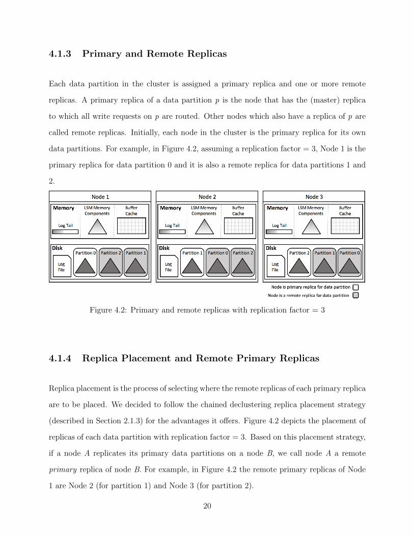
4.1.3 Primary and Remote Replicas

Each data partition in the cluster is assigned a primary replica and one or more remote

replicas. A primary replica of a data partition p is the node that has the (master) replica

to which all write requests on p are routed. Other nodes which also have a replica of p are

called remote replicas. Initially, each node in the cluster is the primary replica for its own

data partitions. For example, in Figure 4.2, assuming a replication factor = 3, Node 1 is the

primary replica for data partition 0 and it is also a remote replica for data partitions 1 and

2.

Figure 4.2: Primary and remote replicas with replication factor = 3

4.1.4 Replica Placement and Remote Primary Replicas

Replica placement is the process of selecting where the remote replicas of each primary replica

are to be placed. We decided to follow the chained declustering replica placement strategy

(described in Section 2.1.3) for the advantages it offers. Figure 4.2 depicts the placement of

replicas of each data partition with replication factor = 3. Based on this placement strategy,

if a node A replicates its primary data partitions on a node B, we call node A a remote

primary replica of node B. For example, in Figure 4.2 the remote primary replicas of Node

1 are Node 2 (for partition 1) and Node 3 (for partition 2).

20

4.2 Implementation of Replication

In this section, we describe how AsterixDB’s data replication protocol is implemented.

4.2.1 Job Replication Protocol

Figure 4.3 shows the sequence of the AsterixDB job replication protocol. In Figure 4.3a, a

client submits a request, which attempts to insert a record r with key k to dataset d that

has a single index I, to the AsterixDB cluster controller. The cluster controller compiles

the request into a Hyracks job (j1 ), then routes the job to the primary replica of the data

partition to which k hashes. The primary replica executes j1, which generates an UPDATE

log record corresponding to record r. After that, the UPDATE log record is added to the

log tail, and record r is added to the memory component of index I. Then, j1 generates an

ENTITY COMMIT log record for record r and appends it to the log tail. Asynchronously, a

log tail Flusher thread forces the log records in the log tail to the log file. At the same time,

a log tail Replicator thread sends the log records in the log tail to each remote replica (by

buffering them in blocks) as shown in the figure. After that, as shown in Figure 4.3b, when

all the log records for j1 have been forced to disk, a local JOB COMMIT log record, which

indicates that all records of j1 have been successfully committed, is added to the log tail.

When the JOB COMMIT log record of j1 is received and also forced to disk by a remote

replica, an ack is sent to the primary replica. Finally, when the JOB COMMIT log record

is forced to disk on the primary replica and acks have been received from all remote replicas,

the client is notified that the submitted request has been completed successfully.

As previously mentioned, in AsterixDB a single job j may try to insert multiple records.

Since these records may be hash-partitioned to different primary replicas, each node should

be able to distinguish between log records of j that belong to the local node and other log

21

(a) Asynchronous job log record replication

(b) Synchronous job completion replication

Figure 4.3: Job replication protocol

records (called remote log records) of remote primary replicas. Similarly, since each node

may have multiple remote primary replicas, it needs to know which log records belong to

which remote primary replica. To achieve this, two additional fields (Log Source and Data

Partition ID) were added to the log record format. Figure 4.4 shows the additional fields’

descriptions.

Log Record Field DescriptionLog Record Source One of the following values:

LOCAL: log was generated by this nodeREMOTE: log was received from a remote primary replica

Data Partition ID The unique data partition ID of the index

Figure 4.4: Additional log fields

22

It is very important to notice that the updates of job j1, in Figure 4.3, are not actually

applied in any of the remote replicas – only their log records were persisted. This has the

following consequences:

1. A memory component for index I need not be allocated in any of the remote replicas.

Therefore, the memory footprint and CPU overhead required for replication are both

minimal.

2. All reads must be routed to the primary replica to avoid stale reads. Therefore, load

balancing of read queries by routing them to remote replicas cannot be supported.

However, since queries in AsterixDB are already load-balanced using hash partitioning

across the cluster nodes, we believe that load balancing of read queries using remote

replicas should not be needed.

3. To perform full recovery in case of a failure, the log records of all committed records

since the last system startup could need to be reapplied on remote replicas. We over-

come this issue by instead replicating LSM disk components as well, as described next.

4.2.2 LSM Disk Component Replication Protocol

In AsterixDB, there are three different operations that result in an LSM disk component

being generated:

1. An index memory component is flushed to disk.

2. Multiple index disk components are merged into a single disk component.

3. An index is initially bulk loaded.

Next, we describe the differences between them and how each case is replicated.

23

Flushed Memory Component Replication

Figure 4.5 shows an example of how flushed LSM memory components are replicated. As

shown in Figure 4.5a, when the memory component of an LSM index reaches a certain

budget, it is flushed to disk. Each disk component contains the local LSN of the last update

operation on the memory component before it was flushed. In addition, it contains a validity

bit that indicates the successful completion of the flush operation. Once the validity bit is set,

the disk component is scheduled for replication by adding a request to a queue that contains

pending replication requests. Asynchronously, a different thread is responsible for processing

the replication requests available in the queue. Since a given logical disk component may

consist of multiple physical files, we need to make sure that all of its files have been received

by each remote replica before declaring the disk component as successfully replicated. To

achieve this, the primary replica starts by sending metadata information about the LSM

component to be replicated such as its index name, number of files, and last update operation

LSN. Upon receiving the metadata information, each remote replica creates an empty mask

file, corresponding to the incoming LSM disk component, to indicate the invalidity of the

component until all of its files have been received. After that, the primary replica sends the

files of the disk component to each remote replica.

Since each node has a single log file with an LSN that grows at a different rate than at

other nodes, the LSNs in the disk components that are received by remote replicas need to

be synchronized to a local LSN value. For example, if the last update operation o on the

memory component on the primary replica had LSN = 1000, a remote replica will receive the

log for operation o and might need to log it locally with LSN = 800. To guarantee that the

AsterixDB recovery algorithm works correctly, the received disk component with LSN = 1000

needs to be updated with LSN = 800. To achieve this, each remote replica must examine

every received log record and maintain a mapping between the remote LSNs (received from

the primary replica) and local LSNs for the last operation per index. In addition, each remote

24

(a) LSM disk component metadata and file replication

(b) Disk component after LSN synchronization

Figure 4.5: Flushed LSM component replication

replica must guarantee that no new log records for an index will be processed until the LSN

value of the disk components have been updated; otherwise, the correct LSN mapping for

that index will be overwritten. To avoid all of this tracking, we instead introduced a new

log record type called FLUSH. Before a primary replica flushes a memory component to

disk, it generates a FLUSH log record. The memory component is then assigned the LSN

of the FLUSH log record instead of the LSN of last update operation. When a log record of

type FLUSH is received by a remote replica, it maintains the mapping between the remote

LSN of the FLUSH log record and the corresponding local FLUSH LSN in a data structure

25

– called the LSN Mapping – in memory. After that, when a disk component is received

from a primary replica, its LSN value is updated to the corresponding local LSN and the

mapping can be removed from the LSN Mapping data structure. As shown in Figure 4.5b,

after all of the files of a disk component have been received and all of its LSNs have been

synchronized, the mask file is deleted on the remote replica to indicate the completion of

the disk component’s replication. When an index’s disk component has successfully been

replicated on a remote replica, it is equivalent to having reapplied all operations on that

index up to the LSN of the disk component. The primary and remote replicas will therefore

be in a mutually consistent state until new operations are applied on the primary replica.

Merged Component Replication

Replicating merged LSM components is similar to replicating flushed memory components.

However, the merged LSM component does not need to generate a FLUSH log record, as

instead it contains the maximum LSN appearing in the merged LSM components. Note

that the LSN mapping for the merged component might not be found in the remote replica

since it may have already been removed from the LSN Mapping data structure in memory.

To overcome this, each replicated index maintains an on-disk LSN Mapping data structure

that is updated with every successful replication of a disk component. When a merged

component is received, its LSN mapping is looked up from its index’s on-disk LSN Mapping

and updated.

In addition to not generating a FLUSH log record, a merged LSM component deletes the

merged disk components after the merge operation is completed. These merged disk com-

ponents need to be deleted from remote replicas but only after the merged component is

replicated successfully. If they are deleted and the primary replica fails before complet-

ing the merged component replication, data will be lost. To avoid this bad situation, the

disk component deletion request is added to the replication request queue after the merged

26

component replication request.

Bulk Loaded Component Replication

AsterixDB allows a new LSM index with no entries to be bulk loaded for the first time

only. The initial bulk load operation does not generate any log records and generates a disk

component with LSN = 0. Replicating a bulk loaded disk component is similar to replicating

a flushed memory component. However, since the bulk load operation does not generate any

log records, in case of a primary replica failure, a bulk loaded disk component cannot be

restored by reapplying its log records. For this reason, bulk loaded disk components are

instead replicated synchronously. Moreover, since bulk loaded components always have a

special LSN of 0, LSN synchronization is not needed on remote replicas since no log records

can have been generated for this index before this disk component.

4.2.3 Replica Checkpointing Coordination

Checkpoints are taken to reduce the time required to perform recovery by making sure that

the disk and memory states are not too far from each other. In AsterixDB, when a certain

amount of log records have been written to the log file, the system tries to move the low-

water mark (the point in the log file that crash recovery starts from) to a higher target value

t by taking a soft (or fuzzy) checkpoint. The checkpoint is taken by noting the smallest LSN

l of all LSM indexes’ memory components (since the effects of any operations with LSN <

l have already been written to a disk component). If some index’s memory component has

a minimum LSN that falls below the target low-water mark value t – called a lagging index

– a flush is initiated, ensuring that its minimum LSN will eventually move to a value > t.

Since remote replicas do not maintain memory components for replicated indexes, we use

the on-disk LSN Mapping data structure to check the minimum local LSN that should be

27

Figure 4.6: Lagging replica index

maintained for each remote replica of an index in order to recover its (primary) in-memory

state if needed due to the loss of its primary replica. Note that it is possible that some

replicated indexes are lagging. In this case, the remote replica cannot flush the index since it

does not have any memory component for it. Figure 4.6 shows an example of this situation.

To overcome this, the remote replica collects the set of lagging indexes per remote primary

replica. A request is then sent to each remote primary replica to flush its lagging indexes.

The primary replica will reply with the same set of lagging indexes and each index will have

one of two possible responses:

1. Index Flushed: this means that the lagging index has a memory component on the

primary replica and a flush has been initiated on the index. Eventually, the newly

flushed disk component will be replicated and its synchronized minimum LSN will

move ahead of the target low-water mark t.

2. Nothing To Flush: this means that the lagging index currently has no memory

component and therefore, no new operations were performed on the index after its

latest disk component. In this case, the remote replica adds a special entry to the

index on-disk LSN Mapping with local LSN = last appended log LSN in the log file

at the time the flush request was sent. This indicates that there are currently no log

records for the lagging index below the target low-water mark t.

28

4.3 Implementation of Fault Tolerance

In this section, we describe how AsterixDB can tolerate node failures and continue to process

requests as long as each data partition has an active replica.

4.3.1 Node Failover

Node failover is the process of moving the services of a failed node to an active node in a

cluster. In AsterixDB, this corresponds to moving the primary replica of a data partition

from a failed node to an active remote replica. To achieve this, we start by maintaining a

list on the cluster controller that contains each data partition, its original storage node, and

the currently assigned primary replica. Figure 4.7 shows an example of the initial state of

this list on an AsterixDB cluster consisting of three nodes each having two data partitions.

When a client request is received on the cluster controller, its compiled job is routed to the

nodes currently assigned as primary replicas.

When a node failure is detected, the cluster controller temporarily stops accepting new

requests and notifies the failed node’s remote replicas as well as its remote primary replicas.

When the node failure notification is received by a remote replica, it deletes any partially

(i.e., in progress) replicated LSM components that belong to the failed node by checking the

existence of mask files. In addition, the remote replica removes any of the failed node’s LSN

mapping information in memory. Similarly, when the failure notification is received by a

remote primary replica, if there is any pending job acknowledgment from the failed node, it

is assumed to have arrived (indicating the end of the job). After that, the remote primary

replica reduces its replication factor.

After sending the failure notification, the cluster controller identifies the data partitions for

which the failed node was the currently assigned primary replica. For each one of these

29

(a) Cluster node controllers

Data Partition ID Original Storage Node Primary Replica0 Node 1 Node 11 Node 1 Node 12 Node 2 Node 23 Node 2 Node 24 Node 3 Node 35 Node 3 Node 3

(b) Cluster state list on the cluster controller

Figure 4.7: Cluster state before any node failures with replication factor = 3

partitions, a partition failover request is sent to an active remote replica. For example, using

the cluster state in Figure 4.7b and assuming a replication factor = 3, if Node 1 fails, a

request might be sent to Node 2 to failover partition 0 and to Node 3 to failover partition 1.

Once a remote replica receives the failover request, it performs the logic shown in Figure 4.8.

As shown in the figure, the remote replica checks the minimum LSN (minLSN ) of all indexes

of the data partition using their on-disk LSN Mapping data structure. After that, all log

records for that data partition with LSN > minLSN are reapplied to catch the remote replica

state up to the same state as the failed primary replica. Next, the data partition’s indexes are

flushed. Finally, the remote replica notifies the cluster controller that the failover request

has been completed. When the cluster controller receives the failover request completion

notification from a remote replica, it updates the cluster state by assigning the remote

replica as the current primary replica for the data partition. Figure 4.9 depicts the cluster

30

state after all failover requests have been completed. When all data partitions once again

have an active primary replica, the cluster starts accepting new requests.

1: dpIndexes← get data partition indexes2: for each index in dpIndexes do3: //find minimum of all maximums4: indexMaxLSN ← index maximum LSN from on-disk LSN Mapping5: dpMinLSN ← min(dpMinLSN, indexMaxLSN)6: end for7: dpLogs← get data partition logs with LSN > dpMinLSN8: Replay dpLogs9: Flush dpIndexes

10: Notify cluster controller

Figure 4.8: Data partition failover logic

It is possible that a remote replica fails before completing a failover request of a data par-

tition, and therefore the request will never be completed. To overcome this problem, a list

of pending failover requests is maintained on the cluster controller. When a remote replica

failure is detected, any pending data partition failover requests that the failed remote replica

was supposed to complete are assigned to different active remote replicas in addition to the

data partitions for which it is the currently assigned primary replica.

4.3.2 Node Failback

Node failback is the process of moving the services of a failed node back to it after it has

repaired or replaced and recovered. In AsterixDB, this corresponds to reassigning the data

partitions of a failed node back to it as the primary replica. When a failed node (the failback

node) first starts up again, a failback process, which consists of initiation, preparation, and

completion stages, must be completed before the node may rejoin the AsterixDB cluster.

The failback process begins in the initiation stage which is performed by the failback node

by following the logic shown in Figure 4.10. As shown, the failback node starts by deleting

31




Figure 4.9: Cluster state after Node 1 partitions failover to Node 2 and Node 3 withreplication factor = 3

any existing data that it might have and then selecting an active remote replica1 to use in

recovery for each data partition. After that, the data partition indexes’ disk components

are copied from each of the selected remote replicas. Finally, the failback node notifies the

cluster controller of its intent to failback. At this point, the initiation stage is completed

and the failback node has all data required for its recovery except for data that might be in

the indexes’ memory components on the data partitions’ primary replicas.

When the cluster controller receives the failback intent notice, the failback node’s failback

process enters the preparation stage which is performed at the cluster level. In this stage, the

cluster controller constructs a failback plan by identifying all nodes that will participate in the

1Currently, the failback node determines active remote replicas by trying to connect to them (based onthe cluster’s intial placement list) during its startup, and it may select any of the active ones during thefailback process.

32

1: delete any existing data2: for each data partition to recover dp do3: remoteReplica← an active remote replica of dp4: get dp LSM indexes disk components from remoteReplica5: end for6: Notify cluster controller of failback intent

Figure 4.10: Node failback initiation logic

failback preparation stage. Those nodes include any remote primary replicas of the failback

node as well as the currently assigned primary replicas for the failback node’s original data

partitions. For example, starting from the cluster state shown in Figure 4.11 and assuming a

replication factor of 3, Node 1’s failback preparation plan would include Node 3 as a remote

primary replica participant, and Node 2 would be a remote primary replica participant in

addition to being the currently assigned primary replica for Node 1’s original data partitions

(partitions 0 and 1). Once the failback preparation plan has been constructed, the cluster

controller enters a re-balancing mode and temporarily halts processing of new requests.

The failback preparation at the cluster level starts when the cluster controller sends a request

to every participant to prepare for the failback. Upon receiving the “prepare for failback”

request, each participant waits for any on-going jobs to complete and then flushes all involved

indexes’ memory components. This step ensures that all indexes of the data partitions that

the failback node should have a copy of have been persisted as disk components. Finally, the

participants notify the cluster controller of their failback preparation request completions.

When all failback preparation plan participants have notified the cluster controller of their

preparation completion, the preparation stage of the failback process is completed and the

cluster controller sends a request to the failback node to complete its failback process’s

completion stage by performing the logic shown in Figure 4.12. In the completion stage, the

failback node starts by copying any disk component which was generated during the failback

preparation stage from an active remote replica for each data partition, as these components

contain the information that the failback node is still missing. After that, the failback node

33




Figure 4.11: Cluster state before Node 1 failback with replication factor = 3

forces its log manager to start up at a new local LSN > all LSNs that appear in any index

disk component. This ensures that all subsequent new jobs’ log records will be replayed

properly in a future failover. Finally, the failback node notifies the cluster controller of the

failback completion.

1: for each data partition to recover dp do2: remoteReplica← an active remote replica of dp3: get dp remaining LSM indexes disk components from remoteReplica4: end for5: force log manager to start from LSN > all disk components’ LSN6: Notify cluster controller of failback completion

Figure 4.12: Node failback completion logic

When the failback completion notification is received on the cluster controller, it notifies

the failback node’s remote primary replicas to reconnect to it and increase their replication

factor. After that, the cluster controller sets the failback node as the primary replica once

34

again for its original data partitions as shown in Figure 4.13. Finally, the cluster leaves the

re-balancing mode and starts accepting new requests again.

Note that during the preparation stage of the failback process, any participant in the failback

preparation plan might fail itself before completing the failback preparation request. In this

case, the plan is canceled and a failover must be performed for the failed participant’s data

partitions. After the failover completion, a new failback plan is constructed. Similarly,

during the failback completion stage, a remote replica might fail before the remaining LSM

disk components can be copied from it. In this situation, a different remote replica is selected

to complete the recover from. However, if the failback node itself fails during any stage of

the failback process, the plan is canceled and the cluster leaves the re-balancing mode and

continues processing requests in its previously degraded state.




Figure 4.13: Cluster state after Node 1 failback with replication factor = 3

35

4.4 Design Discussion

In this section, we describe some of the consequences of using the described replication

protocol in AsterixDB.

4.4.1 Data Inconsistency Window

Recall that AsterixDB essentially supports a record-level read-committed isolation model.

This means if a job j attempts to insert multiple records, once the ENTITY COMMIT log

record of a record r within j is persisted, incoming queries will include r in their result,

even if j “aborts” at a later stage. For efficiency, the described replication protocol works

asynchronously at the record-level and synchronously only at the job level. Therefore, there

is a window of time in which some query may see the record r on the primary replica after

it had been committed locally, but before its log records have been safely received at its

remote replicas. If the primary replica fails during that window, record r will be lost after

the failover process and the query will have observed a state of r that “never was” due to

the failure. This window could be eliminated by changing the AsterixDB isolation model.

Similarly, this window can be minimized at the application level, or the query plan level in

some cases, by limiting the number of records per update job. At this time, however, we

have chosen to educate (warn) AsterixDB users about this behavior.

4.4.2 Temporary Remote Replica Inconsistency

Currently, if a primary replica has more than one active remote replica, log records are

replicated sequentially to each one of them. Therefore, it is possible that some log records

might be sent to one remote replica and the primary replica fails before sending it to others.

This will put remote replicas in a physically inconsistent state. However, note that by the

36

end of the described failover process, the newly assigned primary replica will generate LSM

disk components based on its own log records. Those newly generated disk components

will then be replicated to other remote replicas, bringing all remote replicas of a given data

partition with an active primary replica to a state consistent with that of the new primary

replica.

4.4.3 Node Failover Time Estimation

By following the failover process described earlier, an estimation of the failover time can be

calculated per data partition. During the failback process, in order to generate the additional

disk components needed for the recovery logic in Figure 4.8, a remote replica will have to

apply the log records of the records of indexes’ memory components that were lost on the

failed primary replica. As the memory component size increases, the number of records it can

hold increases and therefore its number of related log records increases. If an average number

of records per memory component can be estimated, the average time needed to replay the

log records of lost memory components can be estimated. In addition to the log records

of its own memory components, if a primary replica fails before completing the replication

of the latest disk component(s) of an index, their log records will have to be applied as

well. However, note that if checkpointing is done frequently, the states of the primary and

remote replicas will be close to each other since disk components will be replicated frequently.

Therefore, if an application has a target maximum tolerable failover time, this target can be

met by configuring the LSM memory component size and checkpointing internal accordingly.

This tuning will be explored further in the next chapter.

37

Chapter 5

Initial Performance Evaluation

In this chapter, we present some initial experimental results to show the impact of As-

terixDB’s replication protocol on the system’s performance. We start by describing the

experimental setup. After that, we compare the performance of AsterixDB using different

replication factors. Finally, we show the time required for the failover and failback processes.

5.1 Experimental Setup

The following experiments have been conducted on a cluster of 7 nodes. The nodes are

Dell PowerEdge 1435SCs with 2 Opteron 2212HE processors, 8 GB DDR2 RAM each, and

two I/O devices of size 1 TB and 7200 RPM speed. An AsterixDB instance is installed on

the cluster. One node is assigned as AsterixDB’s cluster controller and the remaining 6 are

node controllers. Each node controller uses one I/O device for its log file and the other I/O

device for a single data partition. The memory allocated for sort operations is 512 MB.

The memory allocated for disk buffer cache is 3 GB and the memory allocated for a dataset

indexes’ memory component is 1 GB and each memory component’s allocation is divided

38

into two equal parts. Each node controller has 5 reusable log tail buffers of size 6 MB and

6 reusable log tail replication staging buffers of the same size. Log records are buffered in

blocks of size 2 KB when sent to remote replicas.

c r e a t e dataver se Gleambook ;

use dataver se Gleambook ;

c r e a t e type EmploymentType as {o r g a n i z a t i o n : s t r i ng ,s t a r t d a t e : date ,end date : date ?

} ;

c r e a t e type GleambookUserType as {id : int64 ,a l i a s : s t r i ng ,name : s t r i ng ,u s e r s i n c e : datetime ,f r i e n d i d s : {{ i n t64 }} ,employment : [ EmploymentType ]

} ;

c r e a t e datase t GleambookUsers ( GleambookUserType )primary key id ;

Listing 5.1: Experiments dataset definition

The datasets used in the experiments were generated using the AsterixDB SocialGen [5] data

generation tool. Each generated dataset consisted of 6 input files in ADM format that were

divided equally between the node controllers and placed on the same I/O device as its data

partition. All datasets had the same data type, primary key, and a single primary index.

Listing 5.1 shows the AQL statements for defining each dataset. Table 5.1 shows the size

and number of records of each dataset.

39

Number of Records (Million) Size1 384 MB5 1.9 GB10 3.8 GB15 5.8 GB20 7.8 GB

Table 5.1: Experiments’ datasets

5.2 Results and Analysis

5.2.1 Bulk load Time

In this experiment, we evaluate the cost of data replication when bulk loading a dataset

in the case of replication factors of 2 and 3 as compared to a replication factor of 1 (no

replication).

Figure 5.1 shows the results of the experiment on 5 datasets of different sizes (Table 5.1).

From Figure 5.1b, we can see that the bulk load time increased only by an average of 13.4%

in replication factor of 2. This is due to the fact that the bulk load time consists of fetching

and parsing data from external resources, hash partitioning and sorting the records on their

primary keys, bulk loading the records into a newly created partitioned B-Tree index, and

finally writing a single LSM disk component. The additional 13.4% average bulk load time

increase came from replicating the generated disk component to a remote replica. With

a replication factor of 3, however, we can see the bulk load time increased more – by an

average of 47.6%. This is caused by the fact that each primary replica now replicates its

generated disk component to two different remote replicas sequentially. In addition to that,

each remote replica receives two disk components from two different remote primary replicas

simultaneously. This more highly concurrent behavior decreases the likelihood of sequential

writes on the single data partition I/O device. The behavior was not observed with the

replication factor of 2 since each remote replica receives a single disk component in that

40

(a) Bulk load time

(b) Bulk load time increase

Figure 5.1: Bulk load time with different replication factors

case.

5.2.2 Ingestion Time

In this experiment, we evaluate the cost of data replication on different ongoing data ingestion

workloads using replication factors of 2 and 3. The experiment is performed using a local file

system ingestion feed in AsterixDB. This ingestion feed reads a dataset’s records from files

in an input directory, which are split evenly across the dataset’s node controllers (i.e., each

41

node has an input directory that it monitors for incoming data files), and pushes the file’s

records to AsterixDB for ingestion.

(a) Ingestion time

(b) Ingestion time increase

Figure 5.2: Ingestion time with different replication factors

Figure 5.2 shows the results of this experiment using 5 different ingestion workload sizes.

As shown in Figure 5.2b, with a replication factor of 2, the smaller input datasets of 1,

5, and 10 million records had an average ingestion time increase of under 4%. This low

overhead is achieved by maintaining sequential writes on the transaction log file I/O device

as well as the group commit strategy for log writes that AsterixDB utilizes. For the bigger

input datasets of 15 and 20 million records, the average ingestion time increased up to 9.2%.

42

This is due to the fact that as the data gets bigger, LSM memory components reach their

allocated memory budget and are flushed to disk. With every memory component flush, the

generated disk component is replicated. Also, at the same time, a different disk component

is likely being received from a remote primary replica. These concurrent reads and writes on

the data I/O device interfere with memory component flushes and slow them down. With

a replication factor of 3, the average ingestion time increased for the smaller datasets up to

8.1%, which is around double the increase observed with the replication factor of 2. This

is expected due to the fact that each node has to write about two times the number of log

records with replication factor of 2, whereas it has to write around three times the number of

log records for replication factor 3. For the bigger input datasets, the average ingestion time

increase went from up to 9.2% for the replication factor of 2 to up to 13.2% for replication

factor of 3. This is due to the fact that replicating disk components interferes more with

memory component flushes for a longer time period with replication factor of 3. In addition

to this, if the log file I/O device cannot write its log tail buffers to disk fast enough, and all

buffers thus become full, the ingestion job ends up waiting until at least one log tail buffer

is available. The possibility of this happening increases as the duration of the job increases.

5.2.3 Query Response Time

In this experiment, we evaluate the overhead of data replication on concurrent read queries

using replication factors of 2 and 3. The experiment is performed by first bulk loading a

dataset of 15 million records. After that, an ingestion feed is started on a different dataset.

While the ingestion feed is running, the range query shown in Listing 5.2 is executed several

times on the bulk loaded dataset and the average response time is reported.

Figure 5.3 shows the results of the experiment using replication factors of 1, 2, and 3. As

shown in the figure, the average query response time increased by 1.69% and 5.55% for the

43

Figure 5.3: Query response time (dataset size = 15 million records) during ingestion

replication factors of 2 and 3 respectively. This low overhead is actually expected, as read

queries use only the data I/O device while data replication creates additional contention for

this I/O device only during disk component replication. As mentioned earlier, this contention

lasts longer in the case of the replication factor of 3 and therefore replication has a higher

overhead on read queries than for the replication factor of 2.

use dataver se Gleambook ;

l e t $count := count ( f o r $v in datase t GleambookUserswhere $v . id > 100and $v . id < 10000000return $v )

re turn $count ;

Listing 5.2: Range query used during ingestion

5.2.4 Failover and Failback Time

In this experiment, we capture the time taken for node failover and failback using AsterixDB’s

new default replication factor of 3. The experiment is performed by first ingesting a dataset of

a certain size. To capture the worst case scenario, checkpointing is disabled and a node failure

44

is introduced immediately after the ingestion completes. This interrupts the replication

of any disk component that is being replicated at ingestion completion time (or any disk

component that is pending replication). After the node failure is introduced, the elapsed

time taken from node failure detection to failover process completion is reported. Finally, the

failed node is started up again, and the elapsed time from when the failback process starts

until its completion is also reported. To show the impact of the memory component’s size on

the failover and failback times, the experiment was performed using a memory component

size of 1 GB as well as 100 MB. (Note that recovery of the lost memory component’s content

is a major part of the failover process.)

Figure 5.4: Failover time (replication factor = 3, no checkpointing)

Figure 5.4 shows the average failover time on 5 datasets of different sizes for the two memory

component sizes. Overall, the 100 MB memory component size setting always had a better

average failover time. This is due to the fact that memory component flushes occur more

frequently and therefore the lost memory component’s log records that need to be replayed

during the failover process are fewer than in the case of 1 GB memory components. For

the datasets with 15 and 20 million records, the average failover time became significantly

higher than for the smaller datasets in the 1 GB case. This is caused by the fact that some

disk components are pending replication at the time of the failure, and therefore their log

45

records have to be replayed during the failover process. This behavior was not observed

in the 100 MB setting due to the smaller disk component size which requires less time to

replicate compared to the 1 GB disk component size. Note that this gain in failover time in

the case of the 100 MB memory component size, however, comes at the expense of a greater

ingestion time as compared to the 1 GB memory component setting, as shown in Figure 5.5.

The 100 MB case had worse average ingestion times across all dataset sizes due to its more

frequent flushes and merges as compared to the 1 GB case. For this reason, AsterixDB users

will want to carefully set the size of the memory component to meet their tolerable failover

time with a minimum impact on the system’s throughput.

Figure 5.5: Ingestion time with different memory component sizes (replication factor = 3)

To demonstrate the impact of checkpointing on failover time, in addition to the memory

component size, we re-ran the failover experiment on the dataset of 20 million records but

this time checkpointing was enabled. We fixed the memory component size to 1 GB but

used different checkpointing interval sizes of 1 GB and 100 MB (i.e., a soft checkpoint is

performed only if the volume of log records written in the log file since the latest successful

checkpoint is 1 GB or 100 MB). After ingesting the dataset, we introduced a node failure after

5 minutes to allow a checkpoint and any resulting memory components flushes to complete

first. Figure 5.6 shows the results of this experiment. As shown, the 100 MB setting had

46

an average failover time of only 1 second, whereas the 1 GB time was 32 seconds. This

is due to the fact that in the 100 MB case, the checkpoint initiated a flush on the latest

memory component of the dataset and the resulting disk component was replicated to its

remote replicas. Therefore, no log records had to be replayed during the failover. In the

1 GB case however, there was no need to flush the dataset memory component since not

enough log records were written to the log file since the prior checkpoint, thus resulting in a

large number of log records (of the lost memory component) needing to be replayed during

the failover.

Figure 5.6: Checkpoint interval impact on failover time(dataset size = 20 million records, replication factor = 3)

Figure 5.7: Failback time (replication factor = 3)

47

Figure 5.7 shows the failback time results. As expected, the failback times for memory

components of size limits of 1 GB and 100 MB are comparable in most cases since they depend

mostly on the amount of data that needs to be restored on the failback node. However,

Figure 5.7 shows a large difference in the case of the dataset of 15 million records. This is

due to the fact that, during the failback preparation stage, each participant in the failback

plan is asked to flush its memory components’ data to disk before the failback process can

continue. This flush may sometimes result in triggering a merge operation. In this particular

case, the failback process waits until the merge operation is completed. This merge has a

higher probability of happening with the smaller memory component size setting due to

more frequent memory component flushes.

48

Chapter 6

Conclusion and Future Work

6.1 Conclusion

In this thesis, we have described a new AsterixDB data replication protocol that exploits

the properties of LSM-trees. We explained how AsterixDB jobs and LSM disk components

are replicated. We also explained how data consistency guarantees are maintained between

replicas. We then explained how checkpointing is coordinated between replicas. We followed

that by describing how fault tolerance has been built on top of the data replication protocol

and explained how a controllable failover time can be achieved.

This thesis also included an initial performance evaluation of the described data replication

protocol as well as of the fault tolerance processes. We empirically explored the impact

of data replication on AsterixDB’s throughput under different replication factors. We also

showed the overhead of data replication on concurrently executing read queries. Finally, we

explored the replication protocol’s associated failover and failback times and how the LSM

memory component size and the checkpoint interval influence them.

49

6.2 Future Work

6.2.1 Delta Recovery During Failback

Currently, during the failback process, the failback node starts from a clean state and copies

all required data to reach a consistent state with other replicas. This could be improved by

performing a delta recovery where only the missing LSM disk components needed to catch

up with other replicas are requested. However, note that the existing disk components on the

failback node before the failure have LSNs that correspond to it, while the additional disk

components that would be received during the delta recovery have LSNs of remote replicas.

A careful manipulation of LSNs would have to be performed to ensure the correctness of

delta recovery.

6.2.2 Hot Standby Remote Replica

In the described AsterixDB data replication protocol, remote replicas do not actually perform

the updates of jobs received from primary replicas. (These are only performed, if needed, in

the event of a failure.) This has the advantage of not allocating LSM memory components

on remote replicas. However, as a result, during a primary replica failover, the system will

be unusable until a remote replica replays all log records of operations which do not appear

in disk components for a given data partition. This temporary system downtime could be

eliminated by having remote replicas perform the updates of jobs as they are replicated. Note

that this would trade off potentially lower “normal” performance in favor of faster failover in

the event of a failure. Of course, this would also allow the possibility of supporting timeline

consistency reads on remote replicas. It would be interesting to explore these performance

trade-offs further in the future.

50

6.2.3 Cluster Controller Fault Tolerance

Currently, node controller fault tolerance in AsterixDB depends on the cluster controller

being there to coordinate the failover and failback processes between replicas. Similarly,

when a replica fails, the cluster controllers is responsible for notifying the impacted nodes.

If the cluster controller itself fails, however, the cluster becomes usable until the cluster

controller is recovered. This bad situation could be avoided by moving all cluster state

configuration information to a reliable distributed service like ZooKeeper. This way, nodes

could receive cluster state change events from a ZooKeeper service. Similarity, if a cluster

controller fails, its coordination services could be safely and reliably moved to a different

node.

6.2.4 AsterixDB Cluster Scaling

With the introduction of fault tolerance, an AsterixDB cluster that starts with N nodes

may continue to operate with N or fewer nodes as long as there is some active replica for

every data partition. However, adding additional nodes to scale the cluster beyond N nodes

is not supported yet. The APIs that were developed to implement the replication protocol

could potentially be utilized to exchange and repartition data between nodes when additional

nodes are added.

51

Bibliography

[1] Apache Cassandra. http://cassandra.apache.org.

[2] HBase. https://hbase.apache.org.

[3] JSON. http://www.json.org.

[4] MySQL 5.7. http://dev.mysql.com/doc/refman/5.7/en/replication.html.

[5] Socialgen. https://github.com/pouriapirz/socialGen.

[6] Teradata database. http://developer.teradata.com/database.

[7] Tandem database group - NonStop SQL: A distributed, high-performance, high-availability implementation of SQL. In Proceedings of the 2Nd International Work-shop on High Performance Transaction Systems, pages 60–104, London, UK, UK, 1989.Springer-Verlag.

[8] S. Alsubaiee, Y. Altowim, H. Altwaijry, A. Behm, V. Borkar, Y. Bu, M. Carey,I. Cetindil, M. Cheelangi, K. Faraaz, E. Gabrielova, R. Grover, Z. Heilbron, Y.-S.Kim, C. Li, G. Li, J. M. Ok, N. Onose, P. Pirzadeh, V. Tsotras, R. Vernica, J. Wen,and T. Westmann. AsterixDB: A scalable, open source BDMS. Proc. VLDB Endow.,7(14):1905–1916, Oct. 2014.

[9] S. Alsubaiee, A. Behm, V. Borkar, Z. Heilbron, Y.-S. Kim, M. J. Carey, M. Dreseler,and C. Li. Storage management in AsterixDB. Proc. VLDB Endow., 7(10):841–852,June 2014.

[10] D. Bitton and J. Gray. Disk shadowing. In Fourteenth International Conference onVery Large Data Bases, August 29 - September 1, 1988, Los Angeles, California, USA,Proceedings., pages 331–338, 1988.

[11] V. Borkar, M. Carey, R. Grover, N. Onose, and R. Vernica. Hyracks: A flexible andextensible foundation for data-intensive computing. In Proceedings of the 2011 IEEE27th International Conference on Data Engineering, ICDE ’11, pages 1151–1162, Wash-ington, DC, USA, 2011. IEEE Computer Society.

[12] V. Borkar, M. J. Carey, and C. Li. Inside ”big data management”: Ogres, onions, orparfaits? In Proceedings of the 15th International Conference on Extending DatabaseTechnology, EDBT ’12, pages 3–14, New York, NY, USA, 2012. ACM.

52

http://cassandra.apache.org

https://hbase.apache.org

http://www.json.org

http://dev.mysql.com/doc/refman/5.7/en/replication.html

https://github.com/pouriapirz/socialGen

http://developer.teradata.com/database

[13] E. A. Brewer. Towards robust distributed systems (abstract). In Proceedings of theNineteenth Annual ACM Symposium on Principles of Distributed Computing, PODC’00, pages 7–, New York, NY, USA, 2000. ACM.

[14] F. Chang, J. Dean, S. Ghemawat, W. C. Hsieh, D. A. Wallach, M. Burrows, T. Chandra,A. Fikes, and R. E. Gruber. Bigtable: A distributed storage system for structureddata. In Proceedings of the 7th USENIX Symposium on Operating Systems Design andImplementation - Volume 7, OSDI ’06, pages 15–15, Berkeley, CA, USA, 2006. USENIXAssociation.

[15] B. F. Cooper, R. Ramakrishnan, U. Srivastava, A. Silberstein, P. Bohannon, H.-A.Jacobsen, N. Puz, D. Weaver, and R. Yerneni. PNUTS: Yahoo!’s hosted data servingplatform. Proc. VLDB Endow., 1(2):1277–1288, Aug. 2008.

[16] J. Dean and S. Ghemawat. MapReduce: Simplified data processing on large clusters.In Proceedings of the 6th Conference on Symposium on Operating Systems Design &Implementation - Volume 6, OSDI’04, pages 10–10, Berkeley, CA, USA, 2004. USENIXAssociation.

[17] G. DeCandia, D. Hastorun, M. Jampani, G. Kakulapati, A. Lakshman, A. Pilchin,S. Sivasubramanian, P. Vosshall, and W. Vogels. Dynamo: Amazon’s highly availablekey-value store. In Proceedings of Twenty-first ACM SIGOPS Symposium on OperatingSystems Principles, SOSP ’07, pages 205–220, New York, NY, USA, 2007. ACM.

[18] D. DeWitt and J. Gray. Parallel database systems: The future of high performancedatabase systems. Commun. ACM, 35(6):85–98, June 1992.

[19] C. J. Fidge. Timestamps in message-passing systems that preserve the partial ordering.Proceedings of the 11th Australian Computer Science Conference, 10(1):5666, 1988.

[20] S. Ghemawat, H. Gobioff, and S.-T. Leung. The Google file system. In Proceedingsof the Nineteenth ACM Symposium on Operating Systems Principles, SOSP ’03, pages29–43, New York, NY, USA, 2003. ACM.

[21] S. Goel and R. Buyya. Data replication strategies in wide area distributed systems,enterprise service computing: From concept to deployment. In Robin G. Qiu (ed),ISBN 1-599044181-2, Idea Group Inc, pages 211–241, 2006.

[22] J. Gray and A. Reuter. Transaction Processing: Concepts and Techniques. MorganKaufmann Publishers Inc., San Francisco, CA, USA, 1st edition, 1992.

[23] R. Grover and M. J. Carey. Data ingestion in AsterixDB. In Proceedings of the 18thInternational Conference on Extending Database Technology, EDBT 2015, Brussels,Belgium, March 23-27, 2015., pages 605–616, 2015.

[24] H.-I. Hsiao and D. J. DeWitt. Chained declustering: A new availability strategy formultiprocessor database machines. In Proceedings of the Sixth International Conferenceon Data Engineering, pages 456–465, Washington, DC, USA, 1990. IEEE ComputerSociety.

53

[25] H.-I. Hsiao and D. J. DeWitt. A performance study of three high availability datareplication strategies. Distrib. Parallel Databases, 1(1):53–80, Jan. 1993.

[26] P. Hunt, M. Konar, F. P. Junqueira, and B. Reed. ZooKeeper: Wait-free coordinationfor internet-scale systems. In Proceedings of the 2010 USENIX Conference on USENIXAnnual Technical Conference, USENIXATC’10, pages 11–11, Berkeley, CA, USA, 2010.USENIX Association.

[27] D. Karger, E. Lehman, T. Leighton, R. Panigrahy, M. Levine, and D. Lewin. Consistenthashing and random trees: Distributed caching protocols for relieving hot spots on theworld wide web. In Proceedings of the Twenty-ninth Annual ACM Symposium on Theoryof Computing, STOC ’97, pages 654–663, New York, NY, USA, 1997. ACM.

[28] L. Lamport. Paxos made simple, fast, and byzantine. In A. Bui and H. Fouchal, editors,OPODIS, volume 3 of Studia Informatica Universalis, pages 7–9. Suger, Saint-Denis,rue Catulienne, France, 2002.

[29] F. Mattern. Virtual time and global states of distributed systems. In Parallel andDistributed Algorithms, pages 215–226. North-Holland, 1989.

[30] M. K. McKusick and S. Quinlan. GFS: Evolution on fast-forward. Queue, 7(7):10:10–10:20, Aug. 2009.

[31] S. A. Moiz, S. P., V. G., and S. N. Pal. Article: Database replication: A survey ofopen source and commercial tools. International Journal of Computer Applications,13(6):1–8, January 2011. Full text available.

[32] A. Nayak, A. Poriya, and D. Poojary. Article: Type of NoSQL databases and itscomparison with relational databases. International Journal of Applied InformationSystems, 5(4):16–19, March 2013. Published by Foundation of Computer Science, NewYork, USA.

[33] P. O’Neil, E. Cheng, D. Gawlick, and E. O’Neil. The log-structured merge-tree (LSM-tree). Acta Informatica, 33(4):351–385.

[34] J. Rao, E. J. Shekita, and S. Tata. Using Paxos to build a scalable, consistent, andhighly available datastore. Proc. VLDB Endow., 4(4):243–254, Jan. 2011.

[35] K. Shvachko, H. Kuang, S. Radia, and R. Chansler. The Hadoop distributed file system.In Proceedings of the 2010 IEEE 26th Symposium on Mass Storage Systems and Tech-nologies (MSST), MSST ’10, pages 1–10, Washington, DC, USA, 2010. IEEE ComputerSociety.

[36] D. Terry. Replicated data consistency explained through baseball. Commun. ACM,56(12):82–89, Dec. 2013.

54

data replication and fault tolerance in...

Documents