data processing v.3 - phoenix geophysics processing user guide version 3.0 july 2005 •ssmt2000...
TRANSCRIPT

Data ProcessingUser Guide
Version 3.0 July 2005
• SSMT2000 • NPIPlot• MTEditor• Synchro Time Series View
PHOENIX GEOPHYSICS

Data ProcessingUser Guide
Version 3.0 July 2005
• SSMT2000 • NPIPlot• MTEditor• Synchro Time Series View
PHOENIX GEOPHYSICS

Printed in Canada on water resistant Xerox® Laser Never-Tear paper.
This User Guide was created in Adobe FrameMaker 7.0. Writing and Production: Stuart Rogers.
Copyright 2005 Phoenix Geophysics Limited.
All rights reserved. No part of this Guide may be reproduced or transmitted in any form or by any means electronic or mechanical, including photocopying, recording, or information storage and retrieval system, without permission in writing from the publisher. Address requests for permission to:
Phoenix Geophysics Limited, 3781 Victoria Park Avenue, Unit 3, Toronto, ON Canada M1W 3K5, or [email protected].
Information in this document is subject to change without notice.
SSMT2000 and the Phoenix logo are trademarks of Phoenix Geophysics Limited. SyncTSV is a trademark of Anton Kocherov. CompactFlash is a trademark of SanDisk Corporation. Windows and Excel are trademarks of Microsoft Corporation.

i i
Contents
Chapter 1: Introduction . . . . . . . . . . . . . . . . . . . . . . . . . . . 1About this guide . . . . . . . . . . . . . . . . . . . . . . . . 2
Intended audience . . . . . . . . . . . . . . . . . . . . . . 2
About the software. . . . . . . . . . . . . . . . . . . . . . 2SSMT2000. . . . . . . . . . . . . . . . . . . . . . . . . . . . . . . . . 2MT-Editor . . . . . . . . . . . . . . . . . . . . . . . . . . . . . . . . . 2
Synchro Time Series View. . . . . . . . . . . . . . . . . . . . . . 3Installation . . . . . . . . . . . . . . . . . . . . . . . . . . . . . . . . 3
How to get further information and support . . . . . . . . . . . . . . . . . . . . . . . . . . . . . . . . 3
Chapter 2: Data Processing with SSMT2000 . . . . . . . . . . 5Data processing overview . . . . . . . . . . . . . . . 6
Exploring SSMT2000 . . . . . . . . . . . . . . . . . . . . 8Starting SSMT2000 . . . . . . . . . . . . . . . . . . . . . . . . . . 8The main window . . . . . . . . . . . . . . . . . . . . . . . . . . . . 8
Transferring data to your PC . . . . . . . . . . . . . 9Creating folders for your data . . . . . . . . . . . . . . . . . . . 9Copying the files . . . . . . . . . . . . . . . . . . . . . . . . . . . 13Renaming the files . . . . . . . . . . . . . . . . . . . . . . . . . . 15
Verifying site parameters . . . . . . . . . . . . . . .17Understanding the Site Parameter (TBL) file . . . . . . . . .17Editing site parameters with the Multi-table Editor . . . . .18Verifying acquisition times . . . . . . . . . . . . . . . . . . . . .23
Creating Fourier transforms . . . . . . . . . . . . .24
PFT File Naming Convention . . . . . . . . . . . . . . . . . . . .24
Reprocessing the Fourier transforms . . . . .28

ii ii
Batch processing. . . . . . . . . . . . . . . . . . . . . . . 34Editing saved robust parameters . . . . . . . . . . . . . . . . 35
Understanding the magnetotelluric processing parameters . . . . . . . . . . . . . . . . . 36Robust processing parameters . . . . . . . . . . . . . . . . . . 36Crosspower parameters . . . . . . . . . . . . . . . . . . . . . . 38
Understanding Fourier Transform parameters . . . . . . . . . . . . . . . . . . . . . . . . . . . . 39Input Data Type . . . . . . . . . . . . . . . . . . . . . . . . . . . . 39Output Data Format . . . . . . . . . . . . . . . . . . . . . . . . . 41Bands (Levels). . . . . . . . . . . . . . . . . . . . . . . . . . . . . 41Processing Times . . . . . . . . . . . . . . . . . . . . . . . . . . . 42
Examining calibration files. . . . . . . . . . . . . . 42Changing the vertical scale . . . . . . . . . . . . . . . . . . . . 45Printing calibration curves . . . . . . . . . . . . . . . . . . . . . 45Viewing calibration data numerically. . . . . . . . . . . . . . 46
Editing site parameters—advanced . . . . . . 47
Correcting layout errors . . . . . . . . . . . . . . . . .49Preparation . . . . . . . . . . . . . . . . . . . . . . . . . . . . . . . .49Starting layout error correction . . . . . . . . . . . . . . . . . .50Correcting magnetic component connection errors. . . . .52Correcting telluric component errors . . . . . . . . . . . . . .53Revising layout corrections . . . . . . . . . . . . . . . . . . . . .54
Creating reports . . . . . . . . . . . . . . . . . . . . . . . .57The Site Parameters report . . . . . . . . . . . . . . . . . . . . .57The Time Ranges report . . . . . . . . . . . . . . . . . . . . . . .57The Saturated Records report . . . . . . . . . . . . . . . . . . .57The Custom Parameters report . . . . . . . . . . . . . . . . . .60Modifying the Custom Parameters report . . . . . . . . . . .61Opening reports in a spreadsheet program . . . . . . . . . .62
Processing white noise and parallel noise test data. . . . . . . . . . . . . . . . . . . . . . . . . .63Processing orthogonal white noise data . . . . . . . . . . . .63Processing parallel noise data . . . . . . . . . . . . . . . . . . .64

iii iii
Chapter 3: Viewing Noise Test Results with NPIPlot . . 69Starting NPIPlot . . . . . . . . . . . . . . . . . . . . . . . 70
Viewing test results . . . . . . . . . . . . . . . . . . . . 70
Modifying the plot appearance . . . . . . . . . . 72
Printing noise test plots . . . . . . . . . . . . . . . . .72
Evaluating noise test plots . . . . . . . . . . . . . .73
Viewing and exporting channel data . . . . .73
Chapter 4: Editing Processed Data with MT-Editor . . . . 75MT-Editor overview . . . . . . . . . . . . . . . . . . . . 76
Exploring MT-Editor . . . . . . . . . . . . . . . . . . . . 76Starting MT-Editor . . . . . . . . . . . . . . . . . . . . . . . . . . 78The main window . . . . . . . . . . . . . . . . . . . . . . . . . . . 78The menus . . . . . . . . . . . . . . . . . . . . . . . . . . . . . . . 78The Toolbars . . . . . . . . . . . . . . . . . . . . . . . . . . . . . . 80
Setting up export options. . . . . . . . . . . . . . . 84
Starting an editing session . . . . . . . . . . . . . 86Specifying frequencies . . . . . . . . . . . . . . . . . . . . . . . 86Continuing from a previous session . . . . . . . . . . . . . . 88Opening files . . . . . . . . . . . . . . . . . . . . . . . . . . . . . . 88
Viewing the Starting data and Resulting data. . . . . . . . . . . . . . . . . . . . . . . . . . . . . . . . . . . .90Opening the windows . . . . . . . . . . . . . . . . . . . . . . . . .90Choosing parameters and components to view . . . . . . .91Customizing the windows . . . . . . . . . . . . . . . . . . . . . .92Changing graph properties . . . . . . . . . . . . . . . . . . . . .93
Opening and customizing the Editing window . . . . . . . . . . . . . . . . . . . . . . . . . . . . . . . .95Changing graph properties . . . . . . . . . . . . . . . . . . . . .97
Editing the crosspowers . . . . . . . . . . . . . . . . .97
Viewing the data mask . . . . . . . . . . . . . . . . . .99

iv iv
Viewing polar diagrams . . . . . . . . . . . . . . . 101Customizing the polar diagrams window . . . . . . . . . . 101
Printing . . . . . . . . . . . . . . . . . . . . . . . . . . . . . . 102
Saving your work . . . . . . . . . . . . . . . . . . . . . .103
Exporting in EDI format . . . . . . . . . . . . . . . .103
Chapter 5: Viewing Time Series Data with Synchro Time Series View . . . . . . . . . . . . . . . . . . . . . . . 105
Exploring Synchro Time Series View. . . . 106Understanding the main window . . . . . . . . . . . . . . . 106
Viewing time series channels . . . . . . . . . . 108Opening time series files . . . . . . . . . . . . . . . . . . . . . 108Specifying start and end times. . . . . . . . . . . . . . . . . 111Troubleshooting time series files . . . . . . . . . . . . . . . 112
Modifying the time series view. . . . . . . . . 113
Viewing power spectra . . . . . . . . . . . . . . . . .115
Modifying the spectra view . . . . . . . . . . . . .118
Viewing coherencies . . . . . . . . . . . . . . . . . . .120
Printing time series, spectra, and coherency plots . . . . . . . . . . . . . . . . . . . . . . . .121
Appendix A: Data processing flowchart . . . . . . . . . . . . . . . . . . . . . . . . 125

v v
Appendix B: Installing software and setting up your PC . . . . . . . . . . 127System requirements . . . . . . . . . . . . . . . . . 128
Installing the software . . . . . . . . . . . . . . . . 128
Configuring the parallel port . . . . . . . . . . . 130Troubleshooting parallel port communications . . . . . . 133
Updating the software. . . . . . . . . . . . . . . . . 134
Registering MT-Editor . . . . . . . . . . . . . . . . . .135
Organizing your files . . . . . . . . . . . . . . . . . . .136Storing raw data files . . . . . . . . . . . . . . . . . . . . . . . .137Storing calibration files . . . . . . . . . . . . . . . . . . . . . . .138Storing output (plot) files . . . . . . . . . . . . . . . . . . . . .138
Formatting a CompactFlash card . . . . . . . .139
Appendix C: Frequency tables for SSMT2000 . . . . . . . . . . . . . . . . . . . 14150Hz LF, MTU-A, AMTC-30 . . . . . . . . . . . . . . . . . . . 142
50Hz LF, MTU-A, MTC-50 . . . . . . . . . . . . . . . . . . . . 146
50Hz LF, MTU, AMTC-30 (V5-comp.) . . . . . . . . . . . . 150
50Hz LF, MTU, MTC-50 (V5-comp.) . . . . . . . . . . . . . 152
50Hz LF, MTU, MTC-50 (V5-2000) . . . . . . . . . . . . . . 156
60Hz LF, MTU-A, AMTC-30 . . . . . . . . . . . . . . . . . . . .160
60Hz LF, MTU-A, MTC-50 . . . . . . . . . . . . . . . . . . . . .164
60Hz LF, MTU, AMTC-30 (V5-comp.) . . . . . . . . . . . . .168
60Hz LF, MTU, MTC-50 (V5-comp.) . . . . . . . . . . . . . .170
60Hz LF, MTU, MTC-50 (V5-2000) . . . . . . . . . . . . . . .174
Appendix D: System 2000 MTU Family Specifications . . . . . . . . . . . . 179General. . . . . . . . . . . . . . . . . . . . . . . . . . . . . . . 180Channels. . . . . . . . . . . . . . . . . . . . . . . . . . . . . . . . 180Sampling . . . . . . . . . . . . . . . . . . . . . . . . . . . . . . . 180
A/MTU sampling rates. . . . . . . . . . . . . . . . . . . . . . . .180Filtering and noise . . . . . . . . . . . . . . . . . . . . . . . . . .181Clocking and synchronization . . . . . . . . . . . . . . . . . .181
vi vi
Calibration . . . . . . . . . . . . . . . . . . . . . . . . . . . . . . 181Power . . . . . . . . . . . . . . . . . . . . . . . . . . . . . . . . . . 182Scheduling . . . . . . . . . . . . . . . . . . . . . . . . . . . . . . 182Data storage and transfer . . . . . . . . . . . . . . . . . . . . 182
External connections . . . . . . . . . . . . . . . . . . 182Ground . . . . . . . . . . . . . . . . . . . . . . . . . . . . . . . . . 183Telluric inputs . . . . . . . . . . . . . . . . . . . . . . . . . . . . 183Parallel port. . . . . . . . . . . . . . . . . . . . . . . . . . . . . . 183Auxiliary connector. . . . . . . . . . . . . . . . . . . . . . . . . 183Battery connector . . . . . . . . . . . . . . . . . . . . . . . . . 183GPS antenna connector. . . . . . . . . . . . . . . . . . . . . . 183
Mechanical and environmental . . . . . . . . . 183
File types and logical record formats . . . 184Calibration file naming and content . . . . . . . . . . . . . 184
Time series file naming and content . . . . . . . . . . . . . .184Time series file format . . . . . . . . . . . . . . . . . . . . . . .185Time series tag format . . . . . . . . . . . . . . . . . . . . . . .186
Summary of tag byte assignments. . . . . . . . . . . . . . .187
Status codes (Tag Byte 14). . . . . . . . . . . . . . . . . . . .188
Sample rate units (Tag Byte 20) . . . . . . . . . . . . . . . .188
Related products. . . . . . . . . . . . . . . . . . . . . . .189MTU-TXC . . . . . . . . . . . . . . . . . . . . . . . . . . . . . . . .189MTU-2ESD, MTU-5ESD . . . . . . . . . . . . . . . . . . . . . . .189MTU-2ES, MTU-5S . . . . . . . . . . . . . . . . . . . . . . . . . .189MTU-5LR. . . . . . . . . . . . . . . . . . . . . . . . . . . . . . . . .190MTU-AI family . . . . . . . . . . . . . . . . . . . . . . . . . . . . .190
Index . . . . . . . . . . . . . . . . . . . . . . . . . . . . . . . . . . . . . . . . . . . . . . . . . . . . . 191

1 Chapter 1 1
Chapter
Introduction
This chapter provides an introduction to the suite of Phoenix Geophysics MT and AMT data-processing software and tells you about:
• this guide and its intended audience.• how to get further information and support.
2 Chapter 1 About this guide 2
About this guideThis document is a guide to the software used for processing, viewing, and editing time series data acquired by System 2000 and System 2000.net MT and AMT receivers manufactured by Phoenix Geophysics Ltd. Separate chapters cover the different software programs, and appendices provide software installation instructions, tables of frequencies, and system specifications, including a description of file types and record formats.
Intended audienceThis Guide is intended for use by geophysicists and technicians familiar with electromagnetic techniques.
About the softwareFour programs are discussed in this book:
• SSMT2000• NPIPlot• MT-Editor• Synchro Time Series View
SSMT2000
This program takes as input raw time series files, calibration files, and site parameter files. In an intermediate step, it produces Fourier coefficients, which are then reprocessed with data from reference sites, using robust routines. The output is MT Plot files containing multiple crosspowers for each of the frequencies analysed.
NPIPlot
This program allows you to view and print parallel noise test results that have been processed by SSMT2000.

3 Chapter 1 About the software 3
MT-Editor
This program takes as input the MT Plot files created by SSMT2000 and displays the resistivity and phase curves as well as the individual crosspowers that are used to calculate each point on the curves. Crosspowers that were affected by noise can be automatically or manually excluded from the calculations. The program also allows you to display a variety of parameters of the plot files such as tipper magnitude, coherency between channels, and strike direction. The output is industry-standard EDI files suitable for use with geophysical interpretation software such as WinGLink™.
Synchro Time Series View
This program takes as input raw time series files and displays them in graphical format. It can also compute power spectra densities and coherency between channels and display these characteristics in graphical format.
Installation
See Appendix B on page 131 for complete installation and set-up instructions.

4 Chapter 1 How to get further information and support 4
How to get further information and supportContact us at:
Phoenix Geophysics Limited 3781 Victoria Park Avenue, Unit 3Toronto, ONCanada M1W 3K5
Telephone: +1 (416) 491-7340Fax: +1 (416) 491-7378e-mail: [email protected]
Registered customers will be able to access on-line support including FAQs and individual issue-tracking when the renovated Phoenix Web site is launched in mid-to-late 2005.
5 Chapter 1 How to get further information and support 5

6 Chapter 1 How to get further information and support 6

7 Chapter 2 7
Chapter
Data Processing with SSMT2000
This chapter explains how to process the raw data acquired by the MTU⁄MTU-A into a format suitable for geophysical interpretation. Instructions are provided for:
• transferring files to your PC.• verifying parameters.• creating Fourier transforms.• reprocessing the Fourier transforms into crosspowers
using robust routines.
Reference sections at the end of the chapter explain some of the processing parameters in greater detail.

8 Chapter 2 Data processing overview 8
Data processing overviewBefore processing data for the first time, you must install the Phoenix processing software on your computer and prepare your file system and PC desktop. See “Installing the software” on page 132 for complete instructions.
When you process data after each day’s acquisition(s), you will follow this general sequence of steps:
1. Transfer the files from the MTU⁄MTU-A’s CompactFlash™ card to your PC hard drive.
2. Verify and edit the parameters saved in the Site Parameters Table (.TBL) file of each site.
3. Archive the raw data and Site Parameters files (original and edited) on CD-R, DVD, or other storage medium.
4. Create Fourier coefficients from the raw data.
5. Reprocess the Fourier coefficients using a robust reprocessing program and possibly data from one or more reference sites.
6. Edit the resulting crosspowers one frequency at a time to verify the viability of the sounding and to reduce or eliminate low quality data.
7. Translate the edited crosspowers into industry-standard EDI format for use by interpretation software.
You will use the SSMT2000 program to complete steps 1 through 5 and the MT EDIT program to complete steps 6 and 7.
9 Chapter 2 Data processing overview 9
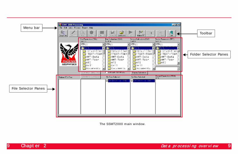
The SSMT2000 main window.
Toolbar
Menu bar
Folder Selector Panes
File Selector Panes
10 Chapter 2 Exploring SSMT2000 10
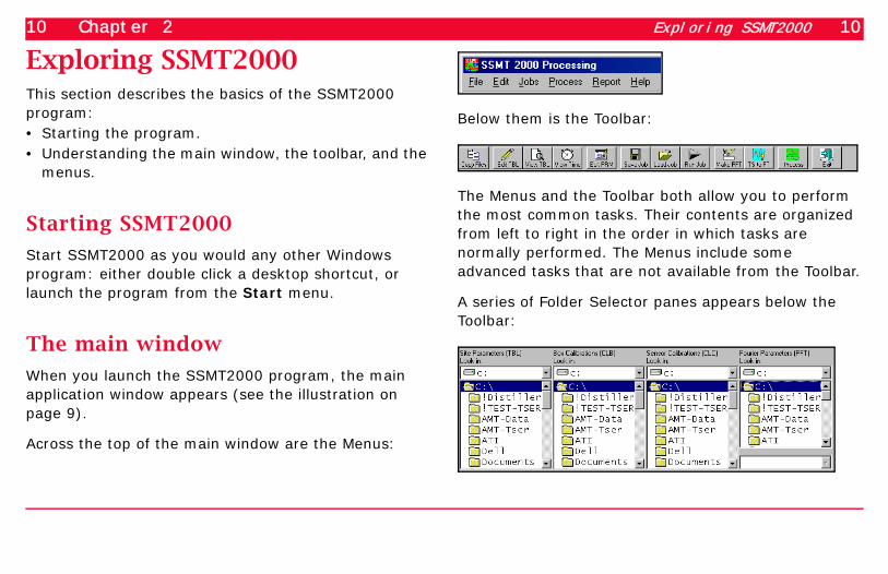
Exploring SSMT2000This section describes the basics of the SSMT2000 program: • Starting the program.• Understanding the main window, the toolbar, and the
menus.
Starting SSMT2000
Start SSMT2000 as you would any other Windows program: either double click a desktop shortcut, or launch the program from the Start menu.
The main window
When you launch the SSMT2000 program, the main application window appears (see the illustration on page 9).
Across the top of the main window are the Menus:
Below them is the Toolbar:
The Menus and the Toolbar both allow you to perform the most common tasks. Their contents are organized from left to right in the order in which tasks are normally performed. The Menus include some advanced tasks that are not available from the Toolbar.
A series of Folder Selector panes appears below the Toolbar:
11 Chapter 2 Transferring data to your PC 11
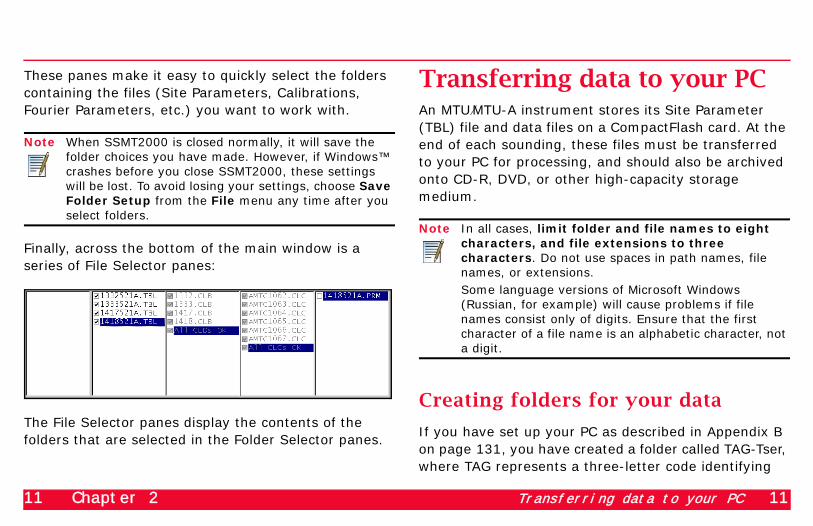
These panes make it easy to quickly select the folders containing the files (Site Parameters, Calibrations, Fourier Parameters, etc.) you want to work with.
Note When SSMT2000 is closed normally, it will save the folder choices you have made. However, if Windows™ crashes before you close SSMT2000, these settings will be lost. To avoid losing your settings, choose Save Folder Setup from the File menu any time after you select folders.
Finally, across the bottom of the main window is a series of File Selector panes:
The File Selector panes display the contents of the folders that are selected in the Folder Selector panes.
Transferring data to your PCAn MTU⁄MTU-A instrument stores its Site Parameter (TBL) file and data files on a CompactFlash card. At the end of each sounding, these files must be transferred to your PC for processing, and should also be archived onto CD-R, DVD, or other high-capacity storage medium.
Note In all cases, limit folder and file names to eight characters, and file extensions to three characters. Do not use spaces in path names, file names, or extensions. Some language versions of Microsoft Windows (Russian, for example) will cause problems if file names consist only of digits. Ensure that the first character of a file name is an alphabetic character, not a digit.
Creating folders for your data
If you have set up your PC as described in Appendix B on page 131, you have created a folder called TAG-Tser, where TAG represents a three-letter code identifying

12 Chapter 2 Transferring data to your PC 12
the survey project. Inside this folder, you will create another folder for each day of acquisition, and store the raw data files in it. This daily folder should be named in the format yyyy-Hdd where:
• “yyyy” represents the year.• “H” represents the month in hexadecimal.• “dd” represents the day of the month in decimal.
For example, data acquired on November 02, 2001, should be stored in a folder named 2001-B02 (November, the eleventh month, is represented by B in hexadecimal) as shown in the illustration.
The raw data file names are based on the serial number of the instrument and the date of the sounding. The format is ssssHdda, with extensions TBL or TS?, where:
• “ssss” represents the serial number of the A/MTU.• “H” represents the month in hexadecimal.• “dd” represents the day of the month in decimal.• “a” represents an alpha character denoting the order
of repeated soundings at a single site.
• “TBL” identifies a Site Parameter file.• “TS?” identifies a time series data file (TSH, TSL, or
TS2 to TS5, depending on instrument firmware).
To create folders for your data files:
1. If you have already created a main (TAG-Tser) folder for your survey, select it from the Site Parameters (TBL) list in the main window:

13 Chapter 2 Transferring data to your PC 13
If you have not created the main folder, select C:\.
2. On the Toolbar, click , or choose Copy Files from the File menu.
The Copy Files dialog box appears. By default, Site parameters and data (TBL, TSn) is already selected, and the Copy to: folder is the one you selected in the main window.

14 Chapter 2 Transferring data to your PC 14
3. If you have already created a main (TAG-Tser) folder for your survey, skip to step 8. If you need to create that folder, continue to step 4.
4. In the Copy to: list at the bottom of the dialog box, select the drive on which you want to store your files.
5. In the folder list at the bottom of the dialog box, double click the root directory (C:\).
6. Click .
The New Folder dialog box appears.
7. Type the name for your main survey folder and click OK.
8. In the folder list at the bottom of the dialog box, double click the main survey folder to open it.
9. Click .
15 Chapter 2 Transferring data to your PC 15
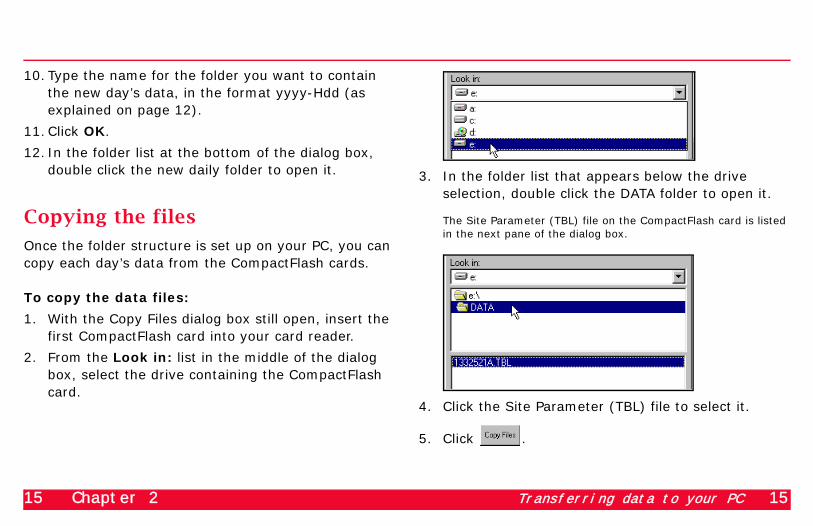
10.Type the name for the folder you want to contain the new day’s data, in the format yyyy-Hdd (as explained on page 12).
11.Click OK.
12. In the folder list at the bottom of the dialog box, double click the new daily folder to open it.
Copying the files
Once the folder structure is set up on your PC, you can copy each day’s data from the CompactFlash cards.
To copy the data files:
1. With the Copy Files dialog box still open, insert the first CompactFlash card into your card reader.
2. From the Look in: list in the middle of the dialog box, select the drive containing the CompactFlash card.
3. In the folder list that appears below the drive selection, double click the DATA folder to open it.
The Site Parameter (TBL) file on the CompactFlash card is listed in the next pane of the dialog box.
4. Click the Site Parameter (TBL) file to select it.
5. Click .

16 Chapter 2 Transferring data to your PC 16
Although only the Site Parameter (TBL) file was selected, SSMT2000 copies all the associated time series files as well as the Site Parameter file.
6. Click OK.
7. To copy data from additional sites, replace the CompactFlash card with one from another site.
8. Right-click anywhere within the Look in: folder listings and click Refresh from the popup menu.
The Site Parameter (TBL) file on the new CompactFlash card is listed.
9. Repeat steps 4 through 8 until you have copied all the day’s data, then close the Copy Files dialog box.
In the main window, SSMT2000 automatically opens the daily data folder and displays a list of the Site Parameter files that have been copied.

17 Chapter 2 Transferring data to your PC 17
Warning! Do not erase the data files from the CompactFlash cards until you are sure the files were copied without error to your hard drive. If you can successfully create Fourier transforms and have archived the data to CD-R, it is usually safe to erase the CompactFlash cards.
Renaming the files
Once the time series and Site Parameter files are copied to your PC, you may want to rename them. The default assigned by the MTU⁄MTU-A is based on the instrument serial number and date, but each instrument will be used many times in a typical survey, making it difficult to relate a raw data file to its site.
Note This procedure is optional. The names of the output files will be created automatically from the Site Name fields in the Site Parameter files. Rename the raw data files only if you want to maintain the naming convention throughout all your files.
If you decide to rename the files, the names will be more meaningful if you base them on a code for the
sites. Phoenix recommends using the pattern TAG-nnna, where:
• “TAG” represents the three-letter code identifying the survey project.
• “nnn” represents the numeric designation of the individual site.
• “a” represents an alpha character denoting the order of repeated soundings at a single site.
If you choose a different naming convention, bear in mind the limits described in the Note on page 11.
SSMT2000 includes a utility that makes it easy to quickly rename many files.
To rename the data files:
1. If any files are selected in the Site Parameters File
Selector pane, click .
2. From the File menu, choose Rename Files.
!

18 Chapter 2 Transferring data to your PC 18
The Rename Files dialog box appears.
3. Select one or more Site Parameter files. (To select multiple files, hold down the SHIFT or CTRL key while clicking.)
4. Click .
The New Name dialog box appears for the first site selected.
5. Consulting the field crew’s Layout Sheet, type the new name in the format TAG-nnna as described on page 12, and click OK.
SSMT2000 renames all files associated with this Site Parameter file, keeping their extensions unchanged.

19 Chapter 2 Verifying site parameters 19
6. If you selected multiple Site Parameter files, SSMT2000 will ask for the new name of the next file in the list. Type the new name and click OK, repeating until all files have been renamed.
7. Click to return to the main window.
Verifying site parametersBefore processing the data files, you need to ensure that the site parameters associated with the data are complete and correct. This section describes how.
Understanding the Site Parameter (TBL) file
The Site Parameter (TBL) file is a record of all the parameters associated with a site’s time series files. However, depending on the firmware of the MTU⁄MTU-A and the set-up method used, some parameter values may not have been recorded automatically. These
values must be added manually before processing can proceed. Normally, the crew will have written the values on the Layout Sheet for the site.
The Site Parameter file is a binary file, and cannot be viewed or edited with a text editor. To edit the contents of the Site Parameter file, you will use SSMT2000’s built-in Multi-table Editor. (To only view the contents of the Site Parameter file, you can use the View TBL button on the Toolbar to create a text file and then read that file with a simple text editor.)
To select Site Parameter files:
• In the File Selector panes, select individual Site Parameter files by clicking the check box next to the file name:

20 Chapter 2 Verifying site parameters 20
• To select all the files, click .
• To clear all the selections, click .
To only review the Site Parameter file(s):
1. On the Toolbar, click , or choose View Site Parameters (TBL) from the Report menu.
A new file with the same name but with the extension .TXT is created in the folder containing the Site Parameter file. Each new .TXT file opens in Notepad.
2. Review the contents of the text file. (Although you can edit this file, the changes will have no effect on processing, since SSMT2000 does not use the file in any way.)
Note Units in the text file may differ from those shown in the Multi-table Editor (volts vs. mvolts, for example).
3. When you have finished reviewing the parameters, close the Notepad window.
Editing site parameters with the Multi-table Editor
SSMT2000 provides an editor that allows you to make changes to several Site Parameter files at once. You can launch the editor from the Toolbar or by choosing Edit Site Parameters (TBL) from the Edit menu.
When you first save a Site Parameter file with the Multi-table Editor, SSMT2000 makes a backup copy of the original file, with the extension TBO. Subsequent saves will not affect the backup file; it remains a copy of the original file.
Note Do not erase TBO files! If errors are made in the editing process and you need to start over, delete the incorrect TBL file. To restore the original Site Parameter file, use the Windows File Rename command to change the TBO file extension back to TBL.
When you launch the editor, the Multi-table Editor window appears:

21 Chapter 2 Verifying site parameters 21
Parameter names Parameter values
Toggle Fields button
Scroll bar

22 Chapter 2 Verifying site parameters 22
Although you can select any number of Site Parameter files, only three can be seen at a time in the editor. If you selected more than three files, use the scroll bar at the bottom of the editor to move among them.
Any of the parameter values that do not appear dimmed can be edited. Use the standard Windows actions and shortcuts to make your changes:• press TAB or SHIFT+TAB to move from field to field.• double click to select a single word.• drag the mouse pointer to select multiple words.• type a new value to replace a selected value.• press CTRL+C to copy a selected value.• press CTRL+V to paste a copied value.
To edit the Site Parameter files:
1. On the Toolbar, click , or choose Edit Site Parameters (TBL) from the Edit menu.
The Multi-table Editing window appears.
2. If desired, click at any time to view more (non-editable) parameters, such as the MTU⁄MTU-A
instrument type, channel configurations, gain
settings, and acquisition times. Click a second time to return to the main editing window.
3. Edit each Site Parameter file for completeness and correctness, using the field crew’s Layout Sheets to find the necessary information.
4. Pay particular attention to the Site Name, since this will be used to name the output (Plot) files.
The Site Name should be in the format SSS-Hdda, where
• “SSS” represents the 3-character site name.
• “H” represents the month in hexadecimal.
• “dd” represents the day of the month in decimal.
• “a” is an alphanumeric character incremented to differentiate multiple output files created by the robust processing routines.
Note If the Site Name field is left blank, SSMT2000 will use the File Name as entered with WinHost in the STARTUP.TBL file, or as created by the MTU⁄MTU-A firmware (using instrument serial number and date).

23 Chapter 2 Verifying site parameters 23
5. Pay particular attention to the values for North Reference, Declination, Ex Azimuth and Hx Azimuth.
Tip The North Reference value is determined by the STARTUP.TBL file used by the MTU⁄MTU-A. If the Reference is Magnetic North, then SSMT2000 will add the Declination to the Ex and Hx Azimuths before processing. However, if the field crew mistakenly aligned the site using a True North Reference, then they have already accounted for Declination in the value they recorded. To compensate for this error, subtract the Declination from the Ex and Hx azimuth values recorded by the crew.On the other hand, if the MTU⁄MTU-A STARTUP file specified True North Reference, then SSMT2000 will ignore the Declination value. If the field crew mistakenly aligned the site using a Magnetic North Reference, you must manually add the Declination to the Ex and Hx Azimuths.
6. Ensure that the Hx, Hy, and Hz serial#s (of a magnetic site) are correct. Delete sensor serial numbers from non-magnetic sites.
(If you’re not sure whether a site used a 2-component or 5-component MTU⁄MTU-A, click
and examine the Channel Config value.)
7. Edit the values for E-line lengths in meters (Ex [N-S] (m) and Ey [E-W] (m)).
8. Edit the values for E-line electrical measurements (Ex and Ey kOhms, AC mV and DC mV).
Note SSMT2000 by default shows a copy of the E-line electrical values measured by the MTU⁄MTU-A. You can safely overwrite the values shown because the MTU⁄MTU-A stores the original values in another (hidden) group of parameters. To see the original values, follow the instructions on page 20 to review the contents of the Site Parameter file, and examine the parameters EXAC, EXDC, EYAC, and EYDC. (Your edited values are in the parameters DXAC, DXDC, DYAC, and DYDC.)
9. When you have finished editing the Site
Parameters, click and close the Multi-table editor.

24 Chapter 2 Verifying site parameters 24
10.Using your archiving or CD-writing software, archive the daily data folder and the related calibration folder on a CD-R or other removable storage medium.
Tip Do not skip the archiving step! The tasks described in this chapter must often be done at the end of the day, when the crew is tired and mistakes are easily made. A few minutes spent here can save an entire day’s work if operator or PC errors occur later on.
Verifying acquisition times
Typically, you will combine data from one or two survey sites with data from a remote reference site in the robust processing stage, in order to reduce the effects of noise. However, only data acquired over the same time span can be combined.
SSMT2000 makes it easy to review the time spans over which data were acquired.
To review data acquisition time spans:
1. In the main window, select the Site Parameter files whose times you want to view.
2. On the Toolbar, click , or choose View Time Ranges from the Report menu.

25 Chapter 2 Creating Fourier transforms 25
The Time Series Ranges dialog box appears. The shaded areas indicate the time spans during which data were acquired.
3. Ensure that the shaded areas overlap sufficiently for good data processing. (If they don’t, you’ll need to choose different sites or acquire more data.)
4. If you have a printer connected to your PC, you can
print the time ranges by clicking .
5. When you are finished reviewing the time ranges, close the dialog box.
Creating Fourier transformsThe next stage in data processing is to produce Fourier transforms from the raw time series data. All sites that are to be processed together must use identical frequency parameters. These parameters are saved in Fourier Transform Parameter (PFT) files, which can be edited if necessary.
As you process data from various surveys, you will build up a library of Fourier Transform Parameter files. At that point you can simply choose an existing file rather than creating a new one.
The Fourier Transform Parameter file names are determined by the parameters saved in the file. Table 2-1 explains the file naming convention.
Table 2-1: PFT File Naming Convention
CharacterPosition
Possible Values
Meaning
1 M, W, P, N Input data type (Measured field, White noise, Parallel noise, parallel white Noise)
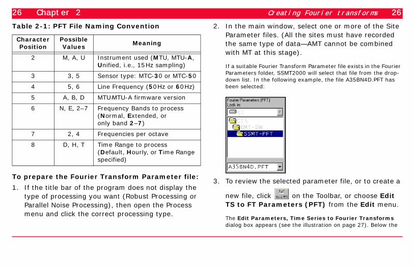
26 Chapter 2 Creating Fourier transforms 26
To prepare the Fourier Transform Parameter file:
1. If the title bar of the program does not display the type of processing you want (Robust Processing or Parallel Noise Processing), then open the Process menu and click the correct processing type.
2. In the main window, select one or more of the Site Parameter files. (All the sites must have recorded the same type of data—AMT cannot be combined with MT at this stage).
If a suitable Fourier Transform Parameter file exists in the Fourier Parameters folder, SSMT2000 will select that file from the drop-down list. In the following example, the file A35BN4D.PFT has been selected:
3. To review the selected parameter file, or to create a
new file, click on the Toolbar, or choose Edit TS to FT Parameters (PFT) from the Edit menu.
The Edit Parameters, Time Series to Fourier Transforms dialog box appears (see the illustration on page 27). Below the
2 M, A, U Instrument used (MTU, MTU-A, Unified, i.e., 15Hz sampling)
3 3, 5 Sensor type: MTC-30 or MTC-50
4 5, 6 Line Frequency (50Hz or 60Hz)
5 A, B, D MTU⁄MTU-A firmware version
6 N, E, 2–7 Frequency Bands to process(Normal, Extended, oronly band 2–7)
7 2, 4 Frequencies per octave
8 D, H, T Time Range to process(Default, Hourly, or Time Range specified)
Table 2-1: PFT File Naming Convention
CharacterPosition
Possible Values
Meaning

27 Chapter 2 Creating Fourier transforms 27
title bar, the dialog box displays the type of data, software version, line frequency filter, and sensor type recorded in the Site Parameter files.
4. For normal processing, none of the settings needs to be changed.
Note It is possible, at the editing and plotting stage, to combine data from MTUs with data from MTU-As. If you want identical frequencies in the overlapping range, set the Output Data Format to two frequencies per octave for all sites.
For orthogonal white noise processing, set the Input Data Type to White noise test. (For more information on processing test data, see “Processing white noise and parallel noise test data” on page 65.)
For advanced processing requirements, see “Under-standing Fourier Transform parameters” on page 41.
5. Save the file and close the dialog box.

28 Chapter 2 Creating Fourier transforms 28
To produce the Fourier transforms:
1. Select the Site Parameter files that you want to work with.
2. On the Toolbar, click , or choose Create Fourier Coefficients (TS to FT) from the Process menu.
SSMT2000 opens a new window and applies Fourier coefficients to the data from each selected Site. The windows close automatically approximately 10s after processing ends:
The results are saved in files with the same name as the Site Parameter file, but with an extension of FCn, where n is the frequency band.
These files are listed in the lower left pane of the main window whenever the associated Site Parameter file is

29 Chapter 2 Reprocessing the Fourier transforms 29
selected. Click the + or – sign to expand or contract the list.
Tip If the Fourier transforms are created without error and you have archived your raw data on CD-R, it is usually safe to erase the CompactFlash cards at this time.
Reprocessing the Fourier transformsThe final calculations applied by SSMT2000 reprocess the Discrete Fourier Transforms (DFTs) into crosspowers. The crosspowers are stored in Plot files that can be displayed graphically and edited using the MTEditor program. This program can also convert crosspowers to industry-standard EDI format for use with geophysical interpretation software. (For more information, see Chapter 4 on page 79.)
The Plot File names are created automatically from the Site Name parameter, with an extension determined by the frequency range. See the MTU Frequency
Ranges chart on page 34 for the three-character extension corresponding to each combination of instrument and sensor type.
If reprocessing is carried out multiple times on the same data, the middle character of the output file extensions will change to a digit, incremented with each repetition.
This stage of processing also allows you to apply a variety of robust routines that can substantially reduce the effect of noise present in the data files.
As with the previous operations, it is first necessary to set up the parameters for this stage of processing.
Note Robust Parameter (PRM) files are unique to each site. They cannot be copied to other folders and used to process other data.
To edit the reprocessing parameters:
1. If the title bar of the program displays SSMT 2000: Parallel Noise Processing, then open the Process menu and click Robust Processing.

30 Chapter 2 Reprocessing the Fourier transforms 30
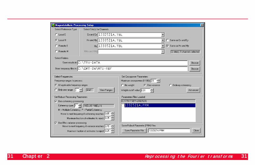
2. On the Toolbar, click or choose Edit Robust Parameters (PRM) from the Edit menu.
The Magnetotelluric Processing Setup dialog box appears:
31 Chapter 2 Reprocessing the Fourier transforms 31

32 Chapter 2 Reprocessing the Fourier transforms 32
3. Select the type of reference channels to be used. Local E or H channels are taken from the site to be processed; Remote E or H channels are taken from another site.
4. Select the site(s) from which you want to take channels. The drop-down lists display the files contained in the Site Parameters folder that was selected in the main window.
If you are processing a 5-component site, you will usually take all the E and H channels from that site,
and take Remote E or H channels from a distant reference site. You can select the 5-component site repeatedly from the drop-down lists, or select Same as Ex and Ey and Same as Hx and Hy.
If you are processing a 2-component site, you will usually take the E channels from that site, the H channels from a nearby 3- or 5-component site, and Remote E or H channels from a distant reference site.
The message box in the Select Site(s) for Channels area confirms the number of different sites and channels selected.
5. Select the folder in which to store the output (Plot) files.
Either locate an existing folder by clicking or type the full path and folder name in the text box. Phoenix recommends using folder names such as
33 Chapter 2 Reprocessing the Fourier transforms 33
“RmH-SITE” (meaning Remote H SITE) or “MTH-SITE” (meaning a Type 4 frequency range—see the chart on page 34) to reflect the type of data and reprocessing.
Note You can type a name for a folder that does not yet exist on your hard drive—SSMT2000 will create the folder during processing. (The folder that is to contain the new folder must already exist, however. SSMT2000 cannot create nested folders.)
6. In the same manner, select the folder in which to store the temporary files that SSMT2000 creates during processing.
Note The temporary files may grow to 500MB in size. Ensure that you have sufficient free disk space to accommodate these files.
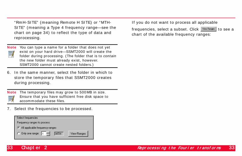
7. Select the frequencies to be processed.
If you do not want to process all applicable
frequencies, select a subset. Click to see a chart of the available frequency ranges:

34 Chapter 2 Reprocessing the Fourier transforms 34
Chart of frequency ranges applicable to each instrument type.
In the chart, find the column for your instrument and sensor type. Note the name of the range
(above the coloured bar) and the number of the range (in braces {}, below the coloured bar). Close the chart and select the number of the range you want to use. See “Frequency tables for SSMT2000” on page 145 for the effect of each choice.
8. If desired, modify the Robust Processing param-eters. See “Robust processing parameters” on page 38 for an explanation of the parameters and their effects.
9. If desired, modify the Crosspower Parameters. See “Crosspower parameters” on page 40 for an expla-nation of the parameters and their effects.

35 Chapter 2 Reprocessing the Fourier transforms 35
• Select the number of crosspowers to be calculated, from 1 to 100.
• Select the weighting factor (No weight, Rho variance, or Ordinary coherency).
• Select the weight cutoff value, from 0.01 to 0.99.
10.When you have finished editing the parameters, save them in a file. SSMT2000 suggests a file name based on the site selected for Ex and Ey channels; however, you can type any file name you want (but see the restrictions in the Note on page 11).
Click to save the settings.
SSMT2000 saves the PRM file to disk, and lists the file in the Parameters Files Loaded list.
11.Click to return to the main window.
To reprocess the Fourier transforms:
1. In the lower right pane of the main window, select the Robust Parameters file that you just prepared.
2. On the Toolbar, click , or choose Process from the Process menu.
SSMT2000 opens a full-screen DOS window and reprocesses the Fourier transforms. This can take several minutes, depending on file sizes. The window closes automatically when reprocessing is finished.
36 Chapter 2 Batch processing 36
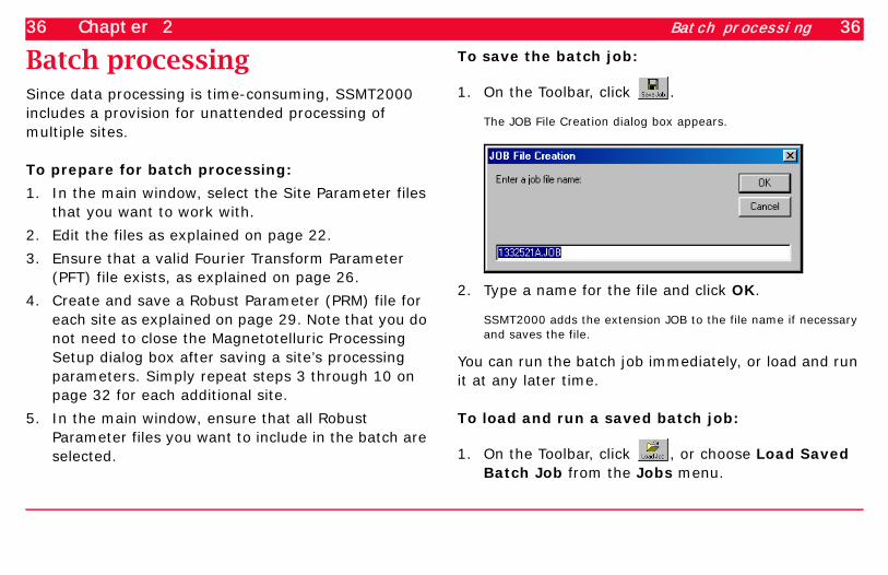
Batch processingSince data processing is time-consuming, SSMT2000 includes a provision for unattended processing of multiple sites.
To prepare for batch processing:
1. In the main window, select the Site Parameter files that you want to work with.
2. Edit the files as explained on page 22.
3. Ensure that a valid Fourier Transform Parameter (PFT) file exists, as explained on page 26.
4. Create and save a Robust Parameter (PRM) file for each site as explained on page 29. Note that you do not need to close the Magnetotelluric Processing Setup dialog box after saving a site’s processing parameters. Simply repeat steps 3 through 10 on page 32 for each additional site.
5. In the main window, ensure that all Robust Parameter files you want to include in the batch are selected.
To save the batch job:
1. On the Toolbar, click .
The JOB File Creation dialog box appears.
2. Type a name for the file and click OK.
SSMT2000 adds the extension JOB to the file name if necessary and saves the file.
You can run the batch job immediately, or load and run it at any later time.
To load and run a saved batch job:
1. On the Toolbar, click , or choose Load Saved Batch Job from the Jobs menu.

37 Chapter 2 Batch processing 37
The Load Batch Job dialog box appears.
2. Select the batch job you want to run from the list of saved JOB files.
3. Click .
4. On the Toolbar, click .
SSMT2000 calculates Fourier transforms for each Site in the JOB file, then reprocesses the data into Plot files.
Editing saved robust parameters
When you have saved the processing parameters for a number of sites, the files will be listed in the Robust Parameters list in the main window:
You can review or change the contents of these files at any time.
To review or edit saved robust reprocessing parameters:
1. On the Toolbar, click or choose Edit Robust Parameters (PRM) from the Edit menu.
The Magnetotelluric Processing Setup dialog box appears.
2. From the Parameters Files Loaded list, click on the name of the file you want to review (it doesn’t matter if the check boxes are selected or cleared—it

38 Chapter 2 Understanding the magnetotelluric processing parameters 38
is the coloured highlight that determines which file will be reviewed).
The Magnetotelluric Processing Setup dialog box is updated to show the parameters saved in the selected file.
3. If you want, change the parameter values and click
.
4. Click to return to the main window.
Understanding the magnetotelluric processing parametersThis section explains the meaning and possible values of the processing parameters in the Magnetotelluric Processing Setup dialog box. The default values should produce satisfactory results in most cases; however, experimentation may improve results in noisy areas.
Robust processing parameters
Two schemes of initial processing that attempt to filter out noise-affected data are controlled by the robust processing parameters: Coherency and Rho variance. This process reduces the size of the error bars and smooths the curves in plots of apparent resistivity.
“Coherency” refers to eight processing schemes that compare survey site data with reference site data, and process only data that are coherent. Cultural noise that is present at the survey site but not at the reference

39 Chapter 2 Understanding the magnetotelluric processing parameters 39
site is therefore reduced (but see the Note on page 40).
“Rho variance” (Resistivity variance) refers to a second stage of coherency processing that compares the telluric and magnetic results from the first stage, and selects data where these results are coherent (again, see the Note on page 40).
Coherency type. This parameter defines which of the eight coherency processing schemes will be used. Enter a value of:
1 to combine Type 2 with Type 3.
2 to use the Multiple Coherency of Ex with the total magnetic field: M(Ex, H).
3 to use the Multiple Coherency of Ey with the total magnetic field: M(Ey, H).
4 to combine Type 5 with Type 6.
5 to use the Partial Coherency of Ex with the total magnetic field: P(Ex, H).
6 to use the Partial Coherency of Ey with the total magnetic field: P(Ey, H).
7 to use the combined factors of the Multiple Coherency of Hx with the total Remote Magnetic field and the Multiple Coherency of Hy with the total Remote Magnetic field: M(Hx, R) * M(Hy, R).
8 to use the combined factors of the Partial Coherency of Hx with the total Remote Magnetic field and the Partial Coherency of Hy with the total Remote Magnetic field: P(Hx, R) * P(Hy, R).
A discussion of Multiple and Partial Coherency is beyond the scope of this guide. Consult a text on statistical methods for a fuller understanding of these terms.
Move to next frequency if coherency (or variance) reaches set value. Even with powerful computers, data processing can be time-consuming. These two parameters define the minimum level of coherency or variance that must be found for the routine to stop processing. Once this minimum level has been found, the program can save time by moving on to the next frequency. Enter a value between 0 and 1.0, where 0 means no coherency and 1.0 means complete coherency.

40 Chapter 2 Understanding the magnetotelluric processing parameters 40
Typical effective values would range from 0.95 for data with much noise to 0.80 for data with little noise.
Maximum fraction of estimates to reject. These two parameters define what fraction of the data can be discarded in each attempt to reach the minimum level of coherency or variance. Enter a value between 0 and 1.0, where 0 means no crosspowers are rejected and 1.0 means all crosspowers can be rejected. Typical effective values would range from 0.75 for data with much noise to 0.25 for data with little noise.
Crosspower parameters
Maximum crosspowers. This is the number of equal-sized segments (maximum 100) into which the time series is divided when calculating data points for each frequency. These data points will be averaged or “stacked” to produce each point on the resistivity and phase curves. If the curves contain large error bars, or are difficult to smooth when editing, it may be helpful to increase the number of crosspowers and reprocess the data.
Weight type (Rho variance, Ordinary coherency). This parameter selects the robust processing scheme used to weight the results of the initial processing described on page 38. Rho variance, the default, gives more weight to data points with smaller error bars. Ordinary coherency gives more weight to data points with good coherency between E and H channels. No weight uses a factor of 1 for all data points and is useful when noise is coherent (see the Note below). Experimentation is the only way to arrive at the best choice for particular survey or site conditions.
Note The same sources of cultural noise may affect both survey and reference sites, and the noise in the data will therefore be coherent. If this is known or suspected to be the case, coherency processing should be disabled so that the noise is not selected for processing.
Weight cutoff value. This parameter affects a step function in the weighting scheme. If the weight factor assigned to a crosspower is less than the weight cutoff value, that weight factor is reduced to zero.

41 Chapter 2 Understanding Fourier Transform parameters 41
Advanced crosspower parameters. On occasion, a survey site will have been laid out in very close alignment to the strike direction, and it is difficult to interpret the results. In this case it is often useful to mathematically rotate the impedance matrix [Z] relative to True North. Enter the desired azimuth in degrees.
Any value other than zero will cause a selection box to appear in the Magnetotelluric Processing Setup dialog box, for easier readjustment of the value.
Understanding Fourier Transform parametersFor normal processing, the default values in the Edit Parameters, Time Series to Fourier Transforms dialog box are correct. This section explains the meaning of the parameters and how to change them for advanced processing requirements.
Input Data Type
Measured field. Select this option for normal processing of field data.
White noise test. A dual random white noise generator is available from Phoenix for bench testing purposes. If data have been acquired with this input, select White noise test to prevent SSMT2000 from attempting to locate and use sensor calibration files. For more information on noise test processing, see “Processing white noise and parallel noise test data” on page 65.

42 Chapter 2 Understanding Fourier Transform parameters 42
Parallel noise test. If the sensors or electrodes were set out in parallel for testing, or if you want to compare similar components from multiple sites, select this checkbox. If the checkbox is selected but unavailable, then the Array Type in the Site Parameter file has been set to 1 – Parallel orientation. For more information on noise test processing, see “Processing white noise and parallel noise test data” on page 65.
Hourly files. Select this option only if the instrument is used in continuous monitoring applications, where the files are closed automatically at set intervals for trans-mission to a processing computer.
43 Chapter 2 Understanding Fourier Transform parameters 43
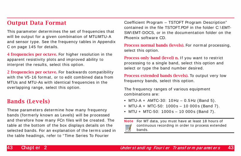
Output Data Format
This parameter determines the set of frequencies that will be output for a given combination of MTU⁄MTU-A and sensor type. See the frequency tables in Appendix C on page 145 for details.
4 frequencies per octave. For higher resolution in the apparent resistivity plots and improved ability to interpret the results, select this option.
2 frequencies per octave. For backwards compatibility with the V5-16 format, or to edit combined data from MTUs and MTU-As with identical frequencies in the overlapping range, select this option.
Bands (Levels)
These parameters determine how many frequency bands (formerly known as Levels) will be processed and therefore how many FCn files will be created. The table at the bottom of the box displays details on the selected bands. For an explanation of the terms used in the table headings, refer to “Time Series To Fourier
Coefficient Program – TSTOFT Program Description” contained in the file TSTOFT.PDF in the folder C:\EMT-SW\EMT-DOCS, or in the documentation folder on the Phoenix software CD.
Process normal bands (levels). For normal processing, select this option.
Process only band (level) n. If you want to restrict processing to a single band, select this option and select or type the band number desired.
Process extended bands (levels). To output very low frequency bands, select this option.
The frequency ranges of various equipment combinations are:
• MTU-A + AMTC-30: 10Hz – 0.5Hz (Band 5).• MTU-A + MTC-50: 1000s – 10 000s (Band 7).• MTU + MTC-50: 1000s – 10 000s (Band 7).
Note For MT data, you must have at least 18 hours of continuous recording in order to process extended bands.

44 Chapter 2 Examining calibration files 44
Processing Times
By default, SSMT2000 processes data acquired over the longest time span common to all the selected sites.
If it is known that data quality is poor at the beginning or end of the common time span—due to a thunderstorm or broken E-lines, for example—better results can be obtained by shortening the time span to eliminate the poor data.
Use default times. Select this option for normal processing.
Specify times. Select this option and edit the Start from or End at times as required to shorten the time span. When you save the parameter file, SSMT2000 will add or increment a digit at the end of the filename, from 0 through 9, to indicate the file version number.
Examining calibration filesPhoenix V-5 System 2000 MTU⁄MTU-As and sensors must be calibrated before each survey and should be
recalibrated at the end of a survey. They may also require recalibration during a survey—in the case of equipment damage, for example.
In the calibration process, the response of the instrument and components is measured using a known input signal. The signal includes components at odd harmonics, starting with a different fundamental for each frequency band the instrument can acquire. The results are stored in a file named with the serial number of the instrument or sensor and the extension .CLB (instrument) or .CLC (sensor).
SSMT2000 includes a utility for viewing and printing different analyses of the calibration results. These analyses will show whether the equipment is working properly. They can also help to verify that you have chosen instrument filter settings that are appropriate for site conditions.
To simply evaluate the calibration, use the DEFAULT.TBL as the Site Parameter File (in step 6 on page 46). This setting removes the effect of the line frequency comb filter. (You can view calibration results

45 Chapter 2 Examining calibration files 45
that include the effect of the filter by selecting a specific Site Parameter file from the list; however, the resulting scatter of points on the curve makes it difficult to evaluate the calibration.)
On the other hand, to evaluate the effect of specific filter settings, select the Site Parameter File containing the settings you want to check. The displayed calibration results will then include the effect of the high-pass filter (if selected) and all digital filters. In the case of an MTU-A, the display will also include the effect of the input low-pass filter, taking into account the electrode resistance as recorded by the user.
Note An inaccurate record of contact resistance will introduce error when the processing software applies its correction using the calibration model. This fact emphasizes the importance of correctly measuring contact resistance at the survey site. Measurements taken at the end of a sounding are preferable to those taken just after the electrodes are buried. (The soil conditions at the electrodes are likely to be unstable for a time after installation, until the salt water has dispersed.)
To view calibration curves:
1. In the SSMT2000 main window, select the folder(s) containing the calibration files you want to examine.
2. Below the Sensor Calibrations (CLC) folder
selector pane, click .
The Display Calibrations dialog box appears.

46 Chapter 2 Examining calibration files 46
3. Select the calibration type (instrument or sensor). If you select Instrument calibrations, you should also select Remove linear phase delay. (Phase delay is an artefact of the digital filters and will disrupt the curves.)
4. From the Select file to display list, select the file you want to view.
5. To view the standard analysis (two frequencies per octave), select the DEFAULT.PFT Fourier Param-
eters File. If you want to view an analysis showing the specific frequencies at which your data will be processed, choose the appropriate Fourier Param-eters File from the dropdown list. (See “Creating Fourier transforms” on page 25 for more infor-mation.)
6. From the Site Parameter File dropdown list, select either DEFAULT.TBL (for simple calibration evaluation) or a specific site TBL file (for filter settings evaluation).
7. Finally, if the calibration was for an MTU-A to acquire MT data (not AMT data), clear the AC coupling checkbox. For other instrument or data types, select AC Coupling.
8. Click .
The Display Calibration Files window appears, showing the magnitude (upper curve) and phase (lower curve) of the instrument or sensor response.

47 Chapter 2 Examining calibration files 47
Changing the vertical scale
By default, the calibration curves are displayed in semi-logarithmic format—the frequency scale (x-axis) is logarithmic and the phase and magnitude scales (y-
axes) are linear. You can toggle the magnitude y-axis between logarithmic and linear scales.
To change the scale of the magnitude curve:
• Right click anywhere on the curves and choose the desired scale from the shortcut menu. (The current choice is indicated by a checkmark.)
Printing calibration curves
If the chart is for a sensor, the calibration is displayed as a single curve.
To print a sensor channel:
• Click either or .
If the chart is for an instrument, multiple channels will be overlaid. Channels are numbered sequentially,

48 Chapter 2 Examining calibration files 48
representing the components in alphabetical order (Ex, Ey, Hx, Hy, Hz, if they exist).
To print a single instrument channel:
• Click one of the Print Channel buttons at the bottom of the window.
To print all the instrument channels overlaid on a single chart:
• Click .
Viewing calibration data numerically
You can view the numerical values of a calibration curve on screen in a spreadsheet format. You can also save or export the data in text (.TXT) or comma separated values (.CSV) format for use by another program. All word processing programs can open .TXT files. Most spreadsheet programs can open .CSV files.
To view raw calibration data:
1. Right click anywhere on the curves and choose View Data from the shortcut menu.
A spreadsheet window displays the data.

49 Chapter 2 Editing site parameters—advanced 49
2. Use the scrollbar on the right of the window to see the remaining frequencies.
To save the data for text editing:
• Click .
A file with the same name but the extension .TXT is saved in the same folder as the calibration file, and the Save to File button appears dimmed.
To export the data for spreadsheet editing:
• Click .
A file with the same name but the extension .CSV is saved in the same folder as the calibration file, and the Export to File button appears dimmed.
Editing site parameters—advancedIn some circumstances, it may be necessary to edit Site Parameters that are not normally changed and are not accessible through the Multi-table Editor. For example, a file may be corrupt and contain an invalid start or end time. It is sometimes possible to overcome such problems using an advanced editing utility that allows direct access to all the fields in a Site Parameter file.
Warning! Modifying parameters incorrectly may produce invalid results, cause data loss, or may prevent data processing altogether. Phoenix Geophysics Ltd. accepts no responsibility for data loss or invalid results or interpretations based on parameters incorrectly modified.DO NOT MODIFY PARAMETERS unless you fully understand the consequences or are advised by Phoenix Geophysics Technical Support.
!
50 Chapter 2 Editing site parameters—advanced 50
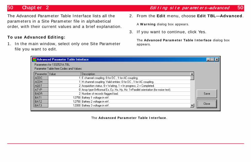
The Advanced Parameter Table Interface lists all the parameters in a Site Parameter file in alphabetical order, with their current values and a brief explanation.
To use Advanced Editing:
1. In the main window, select only one Site Parameter file you want to edit.
2. From the Edit menu, choose Edit TBL—Advanced.
A Warning dialog box appears.
3. If you want to continue, click Yes.
The Advanced Parameter Table Interface dialog box appears.
The Advanced Parameter Table Interface.

51 Chapter 2 Correcting layout errors 51
4. In the Parameter column, locate the required parameter name. Drag the scroll bar on the right if necessary.
5. In the Value column, double click the current value to activate the field.
6. Double click again (or drag the mouse pointer through the value) to select it.
7. Type the new value and press Enter.
8. Repeat as required for other parameters.
9. Click to save the changes or to discard them.
10.Click to return to the main window.
Correcting layout errorsThe most common errors made by inexperienced field crews occur when components are incorrectly oriented, incorrectly connected, or incorrectly identified. If you discover such errors, you can compensate for them
during processing and salvage data that would otherwise be unusable.
Note Users encountering these errors frequently are advised to review the layout procedures described in the V5 System 2000 MTU/MTU-A User Guide.
To correct errors in sensor identification (sensor serial numbers recorded incorrectly), just use the Multi-table editor (see step 6 on page 23) to type in the correct values.
To correct errors in polarity, orientation or connection, use the Edit Layout Errors feature explained here. This feature can correct for:
• Hx, Hy, and/or Hz sensors connected to the wrong terminal on the three-way splitter cable.
• Hx and/or Hy sensors incorrectly oriented by 180°.• Ex and Ey connections interchanged.• Ex and/or Ey polarity reversed.

52 Chapter 2 Correcting layout errors 52
Note It is not practical to try to compensate for incorrectly paired electrodes (e.g., N–E and S–W), since the result is two parallel E-lines instead of two orthogonal E-lines.
Preparation
Before correcting layout errors, use the Multi-table editor to complete the editing of the Site Parameter file in question. Type in all the parameter values necessary, including the ones that you know are wrong, and save the file. This is the starting point for correcting layout errors. If you apply error correction more than once, SSMT2000 must be able to identify this starting point each time.
If you correct layout errors before you have completely edited the Site Parameter file, you will have to use the Multi-table editor on the corrected file. In doing so, you may inadvertently override the corrections. You will also be altering the file from its starting point, making it more difficult to repeat error correction. For these
reasons, you should finish editing with the Multi-table editor before using the Edit Layout Errors feature.
Starting layout error correction
Once you have saved the edited Site Parameter File, you can open the Edit Layout Errors dialog box.
To start layout error correction:
1. In the main window, select only the single Site Parameter file you want to correct.
2. From the Edit menu, choose Layout Errors.
53 Chapter 2 Correcting layout errors 53
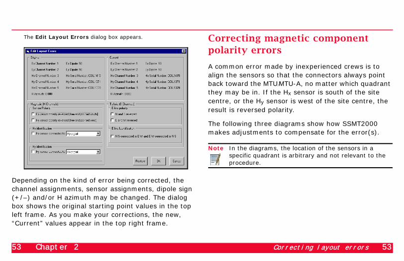
The Edit Layout Errors dialog box appears.
Depending on the kind of error being corrected, the channel assignments, sensor assignments, dipole sign (+/–) and/or H azimuth may be changed. The dialog box shows the original starting point values in the top left frame. As you make your corrections, the new, “Current” values appear in the top right frame.
Correcting magnetic component polarity errors
A common error made by inexperienced crews is to align the sensors so that the connectors always point back toward the MTU⁄MTU-A, no matter which quadrant they may be in. If the Hx sensor is south of the site centre, or the Hy sensor is west of the site centre, the result is reversed polarity.
The following three diagrams show how SSMT2000 makes adjustments to compensate for the error(s).
Note In the diagrams, the location of the sensors in a specific quadrant is arbitrary and not relevant to the procedure.

54 Chapter 2 Correcting layout errors 54
Hx reversed. SSMT2000 interchanges the Hx and Hy channels and serial number assignments and increases the H azimuth by 90°.
Hy reversed. SSMT2000 interchanges the Hx and Hy channels and serial number assignments and decreases the H azimuth by 90°.
Hx and Hy both reversed. SSMT2000 increases the H azimuth by 180° (no change to sensor channels or serial numbers).
To correct for reversed sensor polarity:
1. In the Sensor polarity frame, select either or both check boxes, according to the error that was made.
In the Current frame, SSMT2000 displays adjusted channels, serial numbers, and H azimuth.
This incorrect layout…
…is reinterpreted as this correct layout, rotated 90°.
Hx(ch 3)
Hy (ch 4)
Hx(ch 4)
Hy (ch 3)
90°
This incorrect layout…
…is reinterpreted as this correct layout, rotated –90°.
–90°
Hy (ch 4)
Hx(ch 3)
Hx(ch 4)
Hy (ch 3)
This incorrect layout…
…is reinterpreted as this correct layout, rotated 180°.
180°Hy (ch 4)
Hx(ch 3)
Hx(ch 3)
Hy (ch 4)
55 Chapter 2 Correcting layout errors 55
2. To save the changes, click ; to revert to the
original values, click ; to close the dialog box
without saving changes, click .
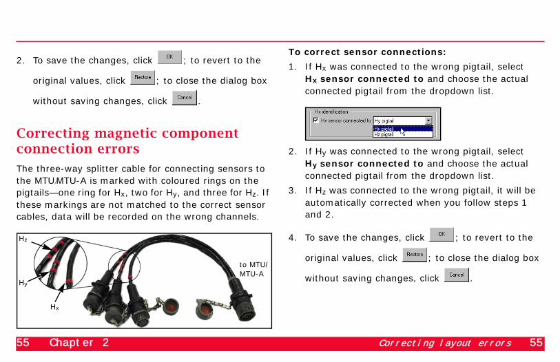
Correcting magnetic component connection errors
The three-way splitter cable for connecting sensors to the MTU⁄MTU-A is marked with coloured rings on the pigtails—one ring for Hx, two for Hy, and three for Hz. If these markings are not matched to the correct sensor cables, data will be recorded on the wrong channels.
To correct sensor connections:
1. If Hx was connected to the wrong pigtail, select Hx sensor connected to and choose the actual connected pigtail from the dropdown list.
2. If Hy was connected to the wrong pigtail, select Hy sensor connected to and choose the actual connected pigtail from the dropdown list.
3. If Hz was connected to the wrong pigtail, it will be automatically corrected when you follow steps 1 and 2.
4. To save the changes, click ; to revert to the
original values, click ; to close the dialog box
without saving changes, click .
Hz
Hy
Hx
to MTU/MTU-A

56 Chapter 2 Correcting layout errors 56
Correcting telluric component errors
Two types of errors in dipole layout can be corrected: reversed polarity of a dipole and interchange of the two dipoles.
Note It is not practical to try to compensate for incorrectly paired electrodes (e.g., N–E and S–W), since the result is two parallel E-lines instead of two orthogonal E-lines.
To correct telluric layout errors:
1. In the Telluric (E Channels) frame, select the check boxes that describe the actual layout conditions.
SSMT2000 corrects polarity by multiplying the dipole length by –1 and corrects interchanged dipoles by interchanging Ex and Ey channel assignments.
2. To save the changes, click ; to revert to the
original values, click ; to close the dialog box
without saving changes, click .
Revising layout corrections
When you make layout error corrections, SSMT2000 saves the original Site Parameter values (the “starting point”) in a special file with the same name but a .TBK extension. This file makes it possible to reverse layout corrections you have made.
To reverse layout corrections:
1. From the Edit menu, choose Layout Errors.
2. Click Restore.
SSMT2000 restores the Site Parameter file to the starting point values.
57 Chapter 2 Correcting layout errors 57
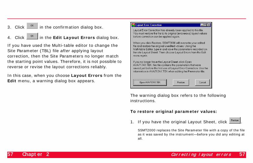
3. Click in the confirmation dialog box.
4. Click in the Edit Layout Errors dialog box.
If you have used the Multi-table editor to change the Site Parameter (TBL) file after applying layout correction, then the Site Parameters no longer match the starting point values. Therefore, it is not possible to reverse or revise the layout corrections reliably.
In this case, when you choose Layout Errors from the Edit menu, a warning dialog box appears.
The warning dialog box refers to the following instructions.
To restore original parameter values:
1. If you have the original Layout Sheet, click .
SSMT2000 replaces the Site Parameter file with a copy of the file as it was saved by the instrument—before you did any editing at all.

58 Chapter 2 Correcting layout errors 58
2. If you don’t have the original Layout Sheet, click Open filename.TBK.
A text version of the Site Parameter file opens in Notepad as it was at the starting point when you first applied layout error correction.
3. Use the Multi-table editor and the Layout Sheet or Notepad file to edit the Site Parameters. If you are using the Notepad file, locate the parameter code in the leftmost column and its value in the rightmost column. The code for each required parameter is shown in the following illustration.

59 Chapter 2 Creating reports 59
Creating reportsFour reports are available from the Report menu:
• Site Parameters• Time Ranges• Saturated Records• Custom Parameters
The Site Parameters report
For information on the Site Parameters report, see “Understanding the Site Parameter (TBL) file” on page 19.
To view the Site Parameters report:
• On the Toolbar, click , or choose View Site Parameters (TBL) from the Report menu.

60 Chapter 2 Creating reports 60
The Time Ranges report
For information on the Time Ranges report, see “Verifying acquisition times” on page 24.
To view the Time Ranges report:
• On the Toolbar, click , or choose View Time Ranges from the Report menu.
The Saturated Records report
The Saturated Records report can be useful when troubleshooting. If Gain is set too high, the dynamic range of the system will be exceeded, resulting in many “saturated” records. A fault in the instrument can also produce this result. The Saturated Records report provides a way of viewing instrument and channel performance for multiple instruments, sites, and channels. The report can be viewed on-screen within SSMT2000 and is simultaneously saved as a comma-separated-values (.CSV) file. Most spreadsheet programs can open or import CSV files, allowing you to
sort the report by various criteria, or manipulate it in other ways.
To create the Saturated Records report:
1. In the Site Parameters folder selection pane, navigate to the folder containing the Site Parameter file(s) you want to include in the report.
A list of the files appears in the Site TBLs file selection pane, but you do not need to select any—the report will cover all files in the folder.

61 Chapter 2 Creating reports 61
2. From the Report menu, choose Saturated Records Report… (If the folder you selected in step 1 contains no Site Parameter files, the command will be unavailable. Repeat step 1, selecting a different folder.)
The Saturated Records Report dialog box appears:
3. Select the records, the sort criterion, and the sort
order, and click .
62 Chapter 2 Creating reports 62
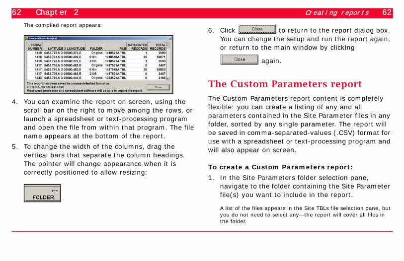
The compiled report appears:
4. You can examine the report on screen, using the scroll bar on the right to move among the rows, or launch a spreadsheet or text-processing program and open the file from within that program. The file name appears at the bottom of the report.
5. To change the width of the columns, drag the vertical bars that separate the column headings. The pointer will change appearance when it is correctly positioned to allow resizing:
6. Click to return to the report dialog box. You can change the setup and run the report again, or return to the main window by clicking
again.
The Custom Parameters report
The Custom Parameters report content is completely flexible: you can create a listing of any and all parameters contained in the Site Parameter files in any folder, sorted by any single parameter. The report will be saved in comma-separated-values (.CSV) format for use with a spreadsheet or text-processing program and will also appear on screen.
To create a Custom Parameters report:
1. In the Site Parameters folder selection pane, navigate to the folder containing the Site Parameter file(s) you want to include in the report.
A list of the files appears in the Site TBLs file selection pane, but you do not need to select any—the report will cover all files in the folder.
63 Chapter 2 Creating reports 63
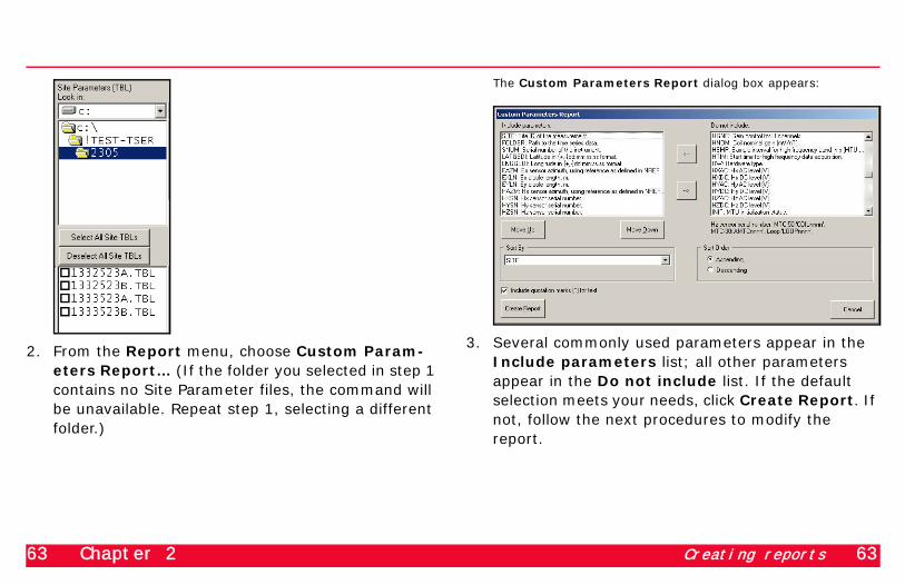
2. From the Report menu, choose Custom Param-eters Report… (If the folder you selected in step 1 contains no Site Parameter files, the command will be unavailable. Repeat step 1, selecting a different folder.)
The Custom Parameters Report dialog box appears:
3. Several commonly used parameters appear in the Include parameters list; all other parameters appear in the Do not include list. If the default selection meets your needs, click Create Report. If not, follow the next procedures to modify the report.

64 Chapter 2 Creating reports 64
Note In the latitude and longitude formats, “d” represents degrees, “m” represents minutes, and “s” represents seconds. “C” represents the cardinal points of the compass—N or S for north or south latitude, E or W for east or west longitude. The EDI format uses a “+” for north or east and a “–” for south or west. The suffixes themselves are acronyms for Degrees/Minutes/ Fractions (DMF), Degrees/ Minutes/Seconds (DMS), and Electronic Data Interchange (EDI).
Modifying the Custom Parameters report
You can add to or subtract from the default list of parameters, and you can change the order of the columns in the report. You can also specify a sorting criterion and sort order.
To remove parameters from the report:
• In the Include parameters list, select the
parameter you want to remove, and click .
The parameter moves from the Include parameters list to the Do not include list.
To add parameters to the report:
• In the Do not include list, select the parameter you
want to include, and click .
The parameter moves from the Do not include list to the bottom of the Include parameters list.
To change the order of included parameters:
• In the Include parameters list, select the parameter you want to move, and click either
or .
To change the sort criteria:
1. After selecting all the parameters you want to include, choose the sort criterion from the Sort By list.
2. Click either the Ascending or Descending sort order.

65 Chapter 2 Processing white noise and parallel noise test data 65
Opening reports in a spreadsheet program
Most word processing and spreadsheet programs can import the report files saved by SSMT2000. The exact procedure will vary depending on the program. As an example, this section provides instructions for using Microsoft Excel™.
To open a report with Microsoft Excel:
1. Launch Excel.
2. In the blank workbook that appears, select cell A1.
3. From the Data menu, point to Import External Data and then click Import Data.
4. In the Files of type list, select All Files (*.*).
5. Select the file saved by SSMT2000 (SATR.CSV, CUSTOM.CSV, or the name you assigned to the file) and click Open.
6. In the Text Import Wizard, click Delimited.
7. Click Next.
8. Select Comma and Space as the Delimiters.
9. Select Treat consecutive delimiters as one.
10.Select " as the Text qualifier.
11.Click Next.
12.Scroll through the Data preview. If any column is empty, select it and click Do not import column (skip).
13.Select the column to the right of the Latitude X Longitude column and click Text.
14.Click Finish.
15. In the Import Data dialog box, click OK to accept cell A1 as the destination.
Processing white noise and parallel noise test dataTwo types of noise tests can be performed to verify or troubleshoot system and component performance: white noise and parallel noise. The processed output from these tests can be viewed and printed with the NPIPlot program.

66 Chapter 2 Processing white noise and parallel noise test data 66
In the case of a white noise test, the input source is a dual random white noise generator, available from Phoenix. The two outputs from the generator can be connected to the MTU⁄MTU-A in either orthogonal or parallel configuration.
In the case of a sensor parallel noise test, one or more MTU⁄MTU-A instruments are set up in the field with the E-lines in parallel at right angles to the sensors, which are also in parallel. You can also conduct parallel tests using multiple standard orthogonal layouts separated by only a meter or so, comparing corresponding channels from two or more instruments.
Processing orthogonal white noise data
White noise data from an orthogonal configuration is processed exactly the same way as normal field data, except that sensor calibration files are not used in the Fourier transform stage of processing.
To process orthogonal white noise data:
• Follow the instructions given earlier in this chapter for processing site data, being sure to select White noise test in the Time Series to Fourier Transform parameters.
Processing parallel noise data
Parallel noise data, whether from a white noise or natural source, is processed differently, so that channels of the same type can be compared with each other, i.e., magnetic with magnetic and telluric with telluric. To view the processed data, use the NPIPlot program, described in Chapter 3 on page 73.
Tip To avoid confusing test data with field data, create a separate folder for the test data and associated Site Parameter files.
Changing the Array type. If you are performing parallel processing on data from a site where the channels were laid out in parallel (i.e., you are not using data

67 Chapter 2 Processing white noise and parallel noise test data 67
from multiple standard orthogonal layouts), the Array Type must be changed in the Site Parameter files.
To change the Array Type:
1. Select the first Site Parameter file containing parallel noise data.
2. From the Edit menu, choose TBL – Advanced… and in the warning dialog box, click Yes to continue.
3. In the Advanced Parameter Table Interface, locate the ATYP parameter and change its value to 1.
4. Save the file and close the Interface.
5. Repeat these steps for any other Site Parameter files you want to process.
Creating Fourier Transforms. The procedure for creating Fourier Transforms is similar to that used for field data.
To prepare the Fourier Transform Parameter file:
1. From the Process menu, choose Parallel Noise Processing.
2. In the folder selection panes of the main window, select the folder containing the Site Parameter files you want to work with.
If a suitable Fourier Transform Parameter file exists in the Fourier Parameters folder, SSMT2000 will select that file from the drop-down list.
3. To review the selected parameter file, or to create a
new file, click on the Toolbar, or choose Edit TS to FT Parameters (PFT) from the Edit menu.
4. If the signal source was a white noise generator, select White noise test as the Input Data Type; otherwise, select Measured Field.
5. Save the file and close the dialog box.

68 Chapter 2 Processing white noise and parallel noise test data 68
To produce the Fourier transforms:
1. Select the Site Parameter files that you want to work with.
2. On the Toolbar, click , or choose Create Fourier Coefficients (TS to FT) from the Process menu.
SSMT2000 opens a new window and applies Fourier coefficients to the data from each selected Site. The windows close automatically approximately 10s after processing ends:
The results are saved in files with the same name as the Site Parameter file, but with an extension of FCn, where n is the frequency band.
These files are listed in the lower left pane of the main window whenever the associated Site Parameter file is

69 Chapter 2 Processing white noise and parallel noise test data 69
selected. Click the + or – sign to expand or contract the list.
Reprocessing the Fourier Transforms. A processing parameters dialog box similar to that for robust processing allows you to set up the channels to be processed.
When you setup these parameters, SSMT2000 will suggest a file name based on the number of E and H channels selected, the date and run number from the first Site Parameter file chosen. For example, if two E-channels and 3 H-channels are selected from Site Parameter file 1332523A.TBL, the file name suggested by SSMT2000 will be E2H3523A.PRM. You can override this suggested file name if you want. The file name of the PRM file will become the file name of the output file, with the extension NPI.
To edit the reprocessing parameters:
1. In the main window folder selection panes, select the folder containing the Site Parameter files you want to work with. (You do not need to select individual files.)
2. On the Toolbar, click or choose Parallel Noise processing (PRM) from the Edit menu.
The Parallel Noise Test Processing Setup dialog box appears.
3. Select the site(s) from which you want to take channels. The drop-down lists display all the files contained in the Site Parameters folder that you selected in the main window.

70 Chapter 2 Processing white noise and parallel noise test data 70
4. Select the E and H channels from each site that you want to process together. You can select up to 7 channels in total.
The message box below the lists confirms the number of different sites and channels selected.
5. Select the folder in which to store the output (Plot) files.
Either locate an existing folder by clicking or type the full path and folder name in the text box.
Note You can type a name for a folder that does not yet exist on your hard drive—SSMT2000 will create the folder during processing. (The folder that is to contain the new folder must already exist, however. SSMT2000 cannot create nested folders.)
6. In the same manner, select the folder in which to store the temporary files that SSMT2000 creates during processing.
7. If desired, overwrite the file name suggested by SSMT2000 for the processing parameters (PRM) file. The file name entered here will be used as the output file name, but with the extension NPI.
8. Save the file and click to return to the main window.
To reprocess the Fourier transforms:
1. In the lower right pane of the main window, select the Robust Parameters file that you just prepared.
2. On the Toolbar, click , or choose Process from the Process menu.
SSMT2000 opens a full-screen DOS window and reprocesses the Fourier transforms. This can take several minutes, depending on file sizes. The window closes automatically when reprocessing is finished.

71 Chapter 2 Processing white noise and parallel noise test data 71
72 Chapter 2 Processing white noise and parallel noise test data 72

73 Chapter 3 73
Chapter
Viewing Noise Test Results withNPIPlot
The NPIPlot program allows you to view and print parallel noise test results that have been processed by SSMT2000.

74 Chapter 3 Starting NPIPlot 74
Starting NPIPlotLaunch the NPIPlot program as you would any Windows program: double click the desktop icon or click Start, point to Programs, then to Phoenix Geophysics NPIPlot, and click NPIPlot.
The main program window appears.
Viewing test resultsYou can view comparisons of any pairs of channels in any of the noise plot files output by SSMT2000.
To select a file for viewing:
1. To locate the folder containing your parallel noise
output files, either click or double click the text box beside it.
2. In the Browse for Folder dialog box, select the folder containing your output files and click OK.
3. In the File list, click the file you want to use.
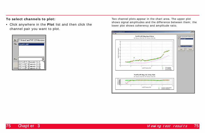
75 Chapter 3 Viewing test results 75
To select channels to plot:
• Click anywhere in the Plot list and then click the channel pair you want to plot.
Two channel plots appear in the chart area. The upper plot shows signal amplitudes and the difference between them; the lower plot shows coherency and amplitude ratio.

76 Chapter 3 Modifying the plot appearance 76
Modifying the plot appearanceThe colours, shapes, and other characteristics of the plot can be customized in several ways.
To modify the plot appearance:
1. Right-click anywhere on the plot and click Appearance.
The Plot Options dialog box appears.
2. Use the controls within the dialog box to customize the appearance of the upper plot.
3. Click or and use the controls to customize the appearance of the lower plot.
4. When you are satisfied, click .
5. If you want to keep these settings as the defaults
for other plots, click .
Printing noise test plotsYou can print each pair of plots individually, or you can print a set of all pairs as a single print job. Each page will be printed in landscape orientation, unless you change the setting from the File menu.
To override the printing defaults:
1. From the File menu, click Print…
2. In the Print dialog box, make the changes you want.

77 Chapter 3 Evaluating noise test plots 77
If you want to add header information such as your company name and address, click Include header, and type the desired information in the Header area.
3. Click .
Note Printing overrides are not saved. If you want to print more plots in the same configuration, repeat the procedure just described; do not use the Print button.
To print using the defaults:
• To print just the pair of plots currently displayed, in
the main window, click .
• To print all the channel pairs, click .
Evaluating noise test plotsAll curves in the plots should be fairly smooth, except at the extremities of the frequency range and at the frequency of the local power grid.
In the lower plot, both the amplitude ratio and coherency should approach 1.0 except at the extremities of the frequency range.
In the upper plot, the signal amplitudes should be roughly a decade above the signal differences.
Viewing and exporting channel dataYou can view the data from the NPI files in a spreadsheet format on screen. You can also export the data from the EDI format to ASCII format files that can then be opened in a word processor or imported to a spreadsheet program.

78 Chapter 3 Viewing and exporting channel data 78
To view or export channel data:
1. Right-click anywhere on the plot you want to export and click View Data.
2. If you want to export the data, click Save To File.
A plain text file with the same name as the NPI file but with the extension ASC is saved in the same folder as the source data.
For an example of how to import report files into spreadsheets, see “Opening reports in a spreadsheet program” on page 65.

79 Chapter 4 79
Chapter
Editing Processed Data withMT-Editor
The output of the SSMT2000 program is one or more files (known as MT Plot files) that form the basis for calculating apparent resistivity and other characteristics of the site. For best results, these files must be edited one frequency at a time, both to verify the viability of the sounding and to reduce or eliminate low quality data.
The edited files can then be translated into various industry-standard EDI formats for use by interpretation software.
Editing and translation is done with the MT-Editor program, described in this chapter.

80 Chapter 4 MT-Editor overview 80
MT-Editor overviewMT-Editor is a Windows-based program that takes as input one or more crosspower (or “plot”) files created by SSMT2000. MT-Editor merges the crosspowers and displays its calculations graphically. This lets you view different characteristics of the soundings, such as apparent resistivity, phase, impedance, strike direction, coherence, and so on, across the full frequency range that was acquired.
MT-Editor also gives you the ability to remove individual crosspowers from the calculations, so that you can edit out poor quality data. The edits are made by changing a mask, not by deleting data, so it is easy to restore individual crosspowers or revert to the initial view. The program includes an “auto-edit” capability that quickly masks crosspowers that lie too far from the mean, saving considerable time in the editing process.
Note To have full functionality, you must register your copy of MT-Editor with Phoenix Geophysics Ltd. You will not be able to save or export your work until the program is registered. See “Registering MT-Editor” on page 139.
Exploring MT-EditorThis section describes the basics of the MT-Editor program: • Starting the program.• Understanding the main window, the toolbars, and
the menus.
The SAMPLE DATA folder on the software distribution CD contains several plot files (*.MT, *.EMT). As you read this chapter, you may want to open these files and experiment with the program features.

81 Chapter 4 Exploring MT-Editor 81
The MT-Editor main window.
Menu bar
Toolbars
Workspace

82 Chapter 4 Exploring MT-Editor 82
Starting MT-Editor
Start MT-Editor as you would any other Windows-based program: either double click a desktop shortcut, or launch the program from the Start menu.
The main window
When you launch the MT-Editor program, the main application window appears (see the illustration on page 81).
Across the top of the main window are the menus:
Below them are the toolbars:
Below the toolbars is the main workspace, in which other windows will open as you work with your files.
The workspace will be blank when you launch the program.
The menus and the toolbars both allow you to perform the most common tasks. The menus include some commands that are not available from the toolbars.
The menus
This section briefly describes each of the seven menus.
Note Individual commands on each menu are disabled and appear dimmed unless a window in which they can be used is open. If a keyboard shortcut exists for a command, it appears to the right of the command on the menu. Menus and commands can also be activated by holding down the Alt key while typing the underlined letter in the menu.
Throughout the instructions in this manual, tools and commands that appear on both a menu and a toolbar are referred to by the toolbar only. It should be understood that menus and keyboard shortcuts can also be used where available.

83 Chapter 4 Exploring MT-Editor 83
The Files menu. The commands on this menu are used to open, close, and export crosspower files; to print the active window contents; to perform automatic editing of several files at once (“batch” processing); and to exit the program. Most of these commands are duplicated on the Files toolbar.
The Edit menu. The two commands on the Edit menu, Deleting and Restoring, toggle the effect of some of the selection tools on the Cursors toolbar, used in editing crosspowers. The commands are duplicated on the EditingMode toolbar.
The View menu. The View commands allow you to switch among various graphical and textual views of the data, and also allow you to show or hide each of the toolbars. All the commands except the Toolbars submenu are duplicated on the View toolbar.
The Processing menu. This menu contains the commands used to automatically or manually edit the crosspowers and to retrieve previous editing sessions. The Options command lets you set the properties of export files such as header text identifying survey participants, distance to the reference site,
measurement units, and EDI format. Most of the Processing commands are duplicated on the Navigate and Processing toolbars.
The Reference menu. The commands on this menu let you switch among four types of calculation that may have been output by SSMT2000, using Local E, Local H, Remote E, or Remote H channels as reference.
The Window menu. The commands on this menu let you organize and rearrange multiple windows that may be open in the main workspace. If the window you want to see is hidden behind others, you can select it from the Window menu to bring it to the front. You can also close all open windows without closing the file(s) you are working with.
The Window commands are not available on a toolbar.
The Help menu. The About command on this menu provides information on the program version and links to the software’s author. The Registration command lets you retrieve and input the coded information that will register the software and enable full functionality.

84 Chapter 4 Exploring MT-Editor 84
For registration instructions, see “Registering MT-Editor” on page 139.
The Toolbars
This section briefly describes the eight toolbars, which provide quick access to the most frequent commands.
Note Individual tools on each toolbar are disabled and appear dimmed unless a window in which they can be used is open.
Hover the mouse pointer over a tool to learn its name and keyboard shortcut, if one exists.
You can customize the main window by showing or hiding individual toolbars, and by rearranging them. This lets you maximize the workspace and the graphs within it.
To show or hide a toolbar:
1. Right-click anywhere in the toolbar area, or choose ToolBars from the View menu.
2. Select the toolbar that you want to show or hide. (Toolbars that are currently showing are indicated by a check mark.)
To move a toolbar:
• Point to the pair of ridges on the left end of the toolbar, and drag it to a new position.
The other toolbars will move as necessary to accommodate the toolbar’s new position.
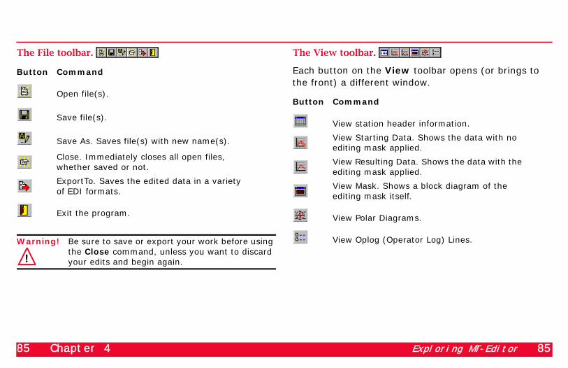
85 Chapter 4 Exploring MT-Editor 85
The File toolbar.
Warning! Be sure to save or export your work before using the Close command, unless you want to discard your edits and begin again.
The View toolbar.
Each button on the View toolbar opens (or brings to the front) a different window.
Button Command
Open file(s).
Save file(s).
Save As. Saves file(s) with new name(s).
Close. Immediately closes all open files, whether saved or not.
ExportTo. Saves the edited data in a variety of EDI formats.
Exit the program.
!
Button Command
View station header information.
View Starting Data. Shows the data with no editing mask applied.
View Resulting Data. Shows the data with the editing mask applied.
View Mask. Shows a block diagram of the editing mask itself.
View Polar Diagrams.
View Oplog (Operator Log) Lines.

86 Chapter 4 Exploring MT-Editor 86
The Processing toolbar.
The buttons on the Processing toolbar open the editing window and also enable the Navigate, Cursors, and EditingMode toolbars.
The Show toolbar.
These tools are only available during editing. Their calculations do not include deleted crosspowers.
The Navigate toolbar.
You can use these tools when editing, to move from one data point to another. However, it is generally more efficient to use the keyboard shortcuts.
Note The spacebar moves leftward or rightward one data point depending on the last direction set by the Prior or Next commands. It also automatically reverses direction when the First or Last data point is encountered.
Button Command
Editing. Opens the editing window and lets you edit crosspowers manually.
AutoEdit. Applies an algorithm to mask outly-ing crosspowers. To see the result, click Edit-ing.
Options. Lets you set up default file proper-ties for exporting in EDI format.
Button Command
Mean view. Shows the arithmetic mean of the crosspowers that make up a given data point.
Std view. Shows ±1 standard deviation of the crosspowers that make up a given data point.
Button Command
First. Moves to the leftmost data point. (Shortcut: CTRL+A.)
Prior. Moves leftward one data point. (Short-cuts: CTRL+S, <spacebar>, or Left Arrow.)
Next. Moves rightward one data point. (Shortcuts: CTRL+D, <spacebar>, or Right Arrow.)
Last. Moves to the rightmost data point. (Shortcut: CTRL+F.)
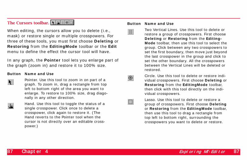
87 Chapter 4 Exploring MT-Editor 87
The Cursors toolbar.
When editing, the cursors allow you to delete (i.e., mask) or restore single or multiple crosspowers. For three of these tools, you must first choose Deleting or Restoring from the EditingMode toolbar or the Edit menu to define the effect the cursor tool will have.
In any graph, the Pointer tool lets you enlarge part of the graph (zoom in) and restore it to 100% size.
Button Name and Use
Pointer. Use this tool to zoom in on part of a graph. To zoom in, drag a rectangle from top left to bottom right of the area you want to enlarge. To restore to 100% size, drag diago-nally in any other direction.
Hand. Use this tool to toggle the status of a single crosspower. Click once to delete a crosspower, click again to restore it. (The Hand reverts to the Pointer tool when the cursor is not directly over an editable cross-power.)
Two Vertical Lines. Use this tool to delete or restore a group of crosspowers. First choose Deleting or Restoring from the Editing-Mode toolbar, then use this tool to select the group. Click between any two crosspowers to set the first boundary, then move just beyond the last crosspower in the group and click to set the other boundary. All the crosspowers between the Vertical Lines will be deleted or restored.
Circle. Use this tool to delete or restore indi-vidual crosspowers. First choose Deleting or Restoring from the EditingMode toolbar, then click with this tool directly on the indi-vidual crosspowers.
Lasso. Use this tool to delete or restore a group of crosspowers. First choose Deleting or Restoring from the EditingMode toolbar, then use this tool to drag a rectangle from top left to bottom right, surrounding the crosspowers you want to delete or restore.
Button Name and Use
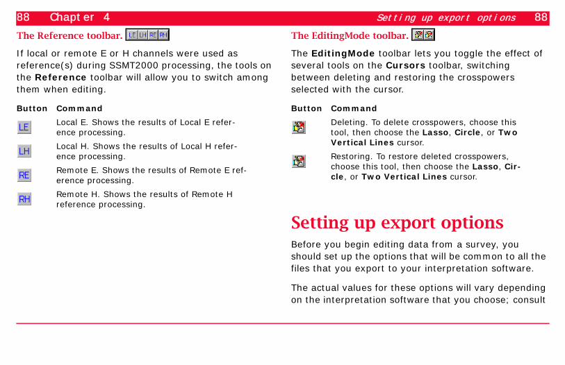
88 Chapter 4 Setting up export options 88
The Reference toolbar.
If local or remote E or H channels were used as reference(s) during SSMT2000 processing, the tools on the Reference toolbar will allow you to switch among them when editing.
The EditingMode toolbar.
The EditingMode toolbar lets you toggle the effect of several tools on the Cursors toolbar, switching between deleting and restoring the crosspowers selected with the cursor.
Setting up export optionsBefore you begin editing data from a survey, you should set up the options that will be common to all the files that you export to your interpretation software.
The actual values for these options will vary depending on the interpretation software that you choose; consult
Button Command
Local E. Shows the results of Local E refer-ence processing.
Local H. Shows the results of Local H refer-ence processing.
Remote E. Shows the results of Remote E ref-erence processing.
Remote H. Shows the results of Remote H reference processing.
Button Command
Deleting. To delete crosspowers, choose this tool, then choose the Lasso, Circle, or Two Vertical Lines cursor.
Restoring. To restore deleted crosspowers, choose this tool, then choose the Lasso, Cir-cle, or Two Vertical Lines cursor.

89 Chapter 4 Setting up export options 89
the software’s documentation to learn what values are appropriate.
To set export options:
1. Click on the Processing toolbar.
The Options dialog appears.
2. Type in the Default data for export to EDI-Files as described above each text box in the dialog.
3. Calculate the average distance in meters between the survey sites and the magnetic reference site, and type in the Remote H distance for reference coils in meters.
4. Make four selections in the Export control area, according to the requirements of your interpre-tation software and the circumstances of your survey:
• Change Arg Z, Rho if your software requires an orientation of the impedance matrix different from the Phoenix standard.
• Choose Measurement Units of either mV/Gamma (H) and mV/km (E) or om (ohm-meters).
• If an additional local Reference was used, choose Additional Loc E, H; otherwise choose Main.
• To export (Write to file) all results in a single continuous file, choose Append; to export results in separate files, choose In New.
90 Chapter 4 Starting an editing session 90
5. Click OK to apply the changes and close the Options dialog.
Starting an editing sessionEvery editing session begins by opening one or more plot files output by SSMT2000. When opening files in MT-Editor, it may be necessary or desirable to specify that only a subset of the data be used. You will also have the choice of continuing with a previously saved editing session, or starting again with the raw data. This section explains how.
Specifying frequencies
The plot files to be edited from a given survey site will vary in content depending on several factors:
• Equipment used (MTU, MTU-A; MTC-50, MTC-30).• Processing parameters chosen in SSMT2000
(Frequency Ranges; Maximum Crosspowers).
It is therefore possible that you will have several files for each site, with each file possibly containing a different number of crosspowers and a different frequency range. MT-Editor allows you to selectively merge the files so that the final output contains the best quality data (up to 100 crosspowers per frequency) and a range of up to 100 frequencies.
For example, data acquired by an MTU-5 using MTC-50 coils could be processed in three ranges of 40 frequencies each: MTH, MTL, and MTR (see the illustration on page 91), with perhaps 40 crosspowers per frequency. MT-Editor could open all three files at once, and for the 20 frequencies in MTL that overlap MTR, all 80 crosspowers would be used to calculate each frequency.
Allowing for the 20 frequencies that overlap, the total number of frequencies for the site would be:
.
A more complex example would be to combine data acquired by an MTU-5A first with MTC-30 coils, then with MTC-50 coils, at a single site. The data could be
3 40×( ) 20– 100=
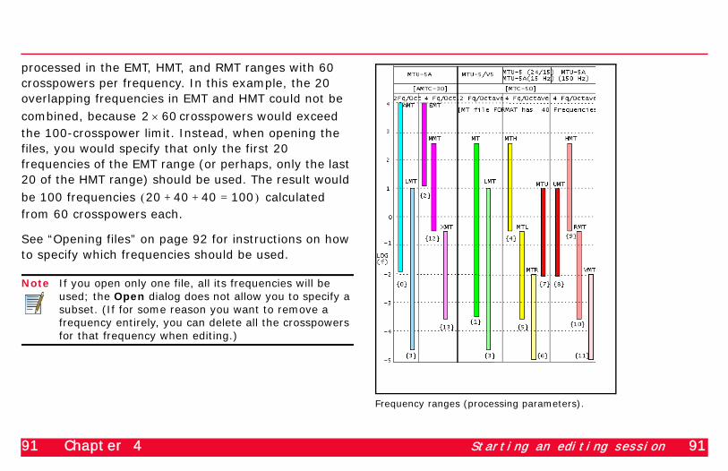
91 Chapter 4 Starting an editing session 91
processed in the EMT, HMT, and RMT ranges with 60 crosspowers per frequency. In this example, the 20 overlapping frequencies in EMT and HMT could not be combined, because crosspowers would exceed the 100-crosspower limit. Instead, when opening the files, you would specify that only the first 20 frequencies of the EMT range (or perhaps, only the last 20 of the HMT range) should be used. The result would be 100 frequencies calculated from 60 crosspowers each.
See “Opening files” on page 92 for instructions on how to specify which frequencies should be used.
Note If you open only one file, all its frequencies will be used; the Open dialog does not allow you to specify a subset. (If for some reason you want to remove a frequency entirely, you can delete all the crosspowers for that frequency when editing.)
Frequency ranges (processing parameters).
2 60×
20 40 40+ + 100=( )

92 Chapter 4 Starting an editing session 92
Continuing from a previous session
When you save your work during an editing session, MT-Editor saves the mask that you create, giving it the name PLOT-EDIT. It does not change the raw data, which is preserved with the name PLOT-COMP. Each new editing session is saved separately. This means that when you open files for editing, you have the choice of starting with the raw data, or continuing from where you left off in a previous session. (You can also revert to previous work during an editing session by choosing Other editing from the Processing menu.)
Opening files
Tip As soon as you open files, the Open menu command and tool are disabled, and remain so until you close the files. If you close all the windows in the main workspace, it may appear that no files are open—yet you cannot use the Open command. In this case, either
re-open the windows for the current files, or click to close the current files and enable the Open command.
To open a single plot file for editing:
1. Click on the Files toolbar.
A standard Windows Open dialog appears.
2. Navigate to the folder containing your plot files, and select the file that you want to edit.
3. Click Open.
If no previous editing session was saved, the Program output window appears briefly, followed by the Starting data window.
If one or more previous editing sessions were saved, a dialog appears with a list of them sorted from earliest to latest.

93 Chapter 4 Starting an editing session 93
4. If you want to start with unedited data, select the line that begins with PLOT-COMP. If you want to continue from a previous session, select one of the lines that begin with PLOT-EDIT.
5. Click OK.
The Program output window appears briefly, followed by the Starting data window.
Note When opening multiple files with mixed reference types, ensure that the first and last files that you select are from sites processed with remote H reference channels. Otherwise, all files will be treated as having local H reference only. (This condition will be removed in a future upgrade of MT-Editor.)
To open multiple plot files for editing:
1. Click on the Files toolbar.
A standard Windows Open dialog appears.
2. Navigate to the folder containing your plot files, and select the files that you want to edit. (Hold down the Ctrl key while clicking to select multiple files.)
3. Click Open.
For each file in turn, a dialog appears with a list of saved editing sessions and two frequency selection boxes.
4. If you want to start with unedited data, select the line that begins with PLOT-COMP. If you want to continue from a previous session, select one of the lines that begin with PLOT-EDIT.
5. If you want to include only a subset of the data, change the frequency number in one or both of the frequency selection boxes. (You can replace the default by selecting it and typing a new number, or
94 Chapter 4 Viewing the Starting data and Resulting data 94
you can click on the up and down arrows to scroll through the list.)
6. Click OK.
Tip When files contain overlapping frequencies, it can be valuable to first open them separately, to find out which contain the best quality data at various frequencies. Then when you merge the files for editing, you can specify which frequencies to use from each.
Viewing the Starting data and Resulting dataBecause MT-Editor uses a mask to “delete” crosspowers, it is always possible to view both the results of your edits and the data you started with. Two different windows display these views: the Starting data window and the Resulting data window.
Opening the windows
When you first open files, MT-Editor performs a series of calculations in the Program output window, and then opens the Starting data window automatically. If you close this window, you can reopen it from the toolbar.
To open the the Resulting data window:
• Click on the View toolbar.
To reopen the Starting data window:
• Click on the View toolbar.

95 Chapter 4 Viewing the Starting data and Resulting data 95
The Starting data window.
Tip When multiple windows are open, you can bring a hidden window into view by choosing it from the Window menu.
Choosing parameters and components to view
The Starting data and Resulting data windows allow you to view nine different parameters of the plot files:
As you select each parameter, the Components list will change appropriately, allowing you to select which components are displayed. By default, all components, processing methods, and files for the displayed parameter are selected when you first open the window.

96 Chapter 4 Viewing the Starting data and Resulting data 96
To toggle the display of components, files, processing methods, or legends:
• Select or clear the the item in the control area lists that you want to display or hide. A checkmark indicates that an item is displayed.
Tip Viewed on screen, the control areas of the Resulting data window make clear what components the markers represent. However, the control areas will not appear in a printout. To produce a meaningful printout, select Show legend before printing.
Customizing the windows
You can customize the appearance of the Starting data and Resulting data windows in a variety of ways. MT-Editor saves the customizations between launches. Even if you don’t customize, though, choosing different files, parameters, and window sizes may result in windows or window controls being
clipped. This section explains how to manage the windows’ appearance.
Moving and resizing windows. Use standard Windows mouse commands to change a window’s size and position: move a window by dragging its title bar; maximize it by clicking the Maximize button; resize or reshape it by dragging the corners or sides.
Resizing or restoring window controls. The right hand side of each Starting data or Resulting data window contains a set of controls for choosing the parameter to display, as well as for selecting which components, files, processing types, and legends should be visible. See “Choosing parameters and components to view” on page 95 for instructions on using these controls.
If more choices are available than can fit into a control list, a scroll bar will appear to the right of the list. Depending on the the number of files, channels, or components available, it may be helpful to resize a control area to avoid the need to scroll. Furthermore, if you resize the whole window, you may find that some of the controls are clipped at the bottom. Resizing any control area will restore the clipped areas.
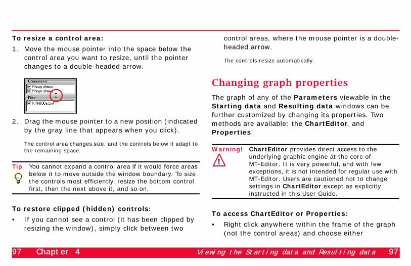
97 Chapter 4 Viewing the Starting data and Resulting data 97
To resize a control area:
1. Move the mouse pointer into the space below the control area you want to resize, until the pointer changes to a double-headed arrow.
2. Drag the mouse pointer to a new position (indicated by the gray line that appears when you click).
The control area changes size, and the controls below it adapt to the remaining space.
Tip You cannot expand a control area if it would force areas below it to move outside the window boundary. To size the controls most efficiently, resize the bottom control first, then the next above it, and so on.
To restore clipped (hidden) controls:
• If you cannot see a control (it has been clipped by resizing the window), simply click between two
control areas, where the mouse pointer is a double-headed arrow.
The controls resize automatically.
Changing graph properties
The graph of any of the Parameters viewable in the Starting data and Resulting data windows can be further customized by changing its properties. Two methods are available: the ChartEditor, and Properties.
Warning! ChartEditor provides direct access to the underlying graphic engine at the core of MT-Editor. It is very powerful, and with few exceptions, it is not intended for regular use with MT-Editor. Users are cautioned not to change settings in ChartEditor except as explicitly instructed in this User Guide.
To access ChartEditor or Properties:
• Right click anywhere within the frame of the graph (not the control areas) and choose either
!

98 Chapter 4 Viewing the Starting data and Resulting data 98
ChartEditor or Properties from the popup menu, as noted in the instructions that follow.
To optimize the x-axis:
1. Choose Properties from the popup menu.
2. Select AutoX.
3. Click to apply the change and close the dialog.
The scale adjusts to fit all the data points into the entire horizontal axis.
To change axis scales manually:
1. Choose Properties from the popup menu.
2. Click on the Min or Max value you want to change and type a new value.
3. If you are changing the horizontal scale, clear AutoX.
4. Click to apply the change and close the dialog.
Tip The default scales for most graphs should be adequate, however, you will probably want to set the values for Tipper magnitude to a minimum of 0.01 and a maximum of 1.0.
It is best to use non-zero values in all fields. Minimum values of 0.0 for any graph may cause all points to disappear from view.
To change marker size for all points:
1. Choose Properties from the popup menu.
2. Click on PointSize and type a new value.
The size of the markers for all data points changes to the new value.
3. Click to apply the change and close the dialog.

99 Chapter 4 Opening and customizing the Editing window 99
To change marker properties for only one component:
1. Choose ChartEditor from the popup menu.
2. Click the Series tab.
3. Select the component from the drop-down list.
4. Select a new marker Style, Width, and/or Height.
5. Close the ChartEditor.
Note Changing PointSize in the Properties dialog will reset all the markers to their default shapes and the current point size.
To add a line between points:
1. Choose Properties from the popup menu.
2. Select Line.
The graph style changes from markers only to line plus markers.
Opening and customizing the Editing window
To open the editing window:
1. If you want to use Autoediting, click on the Processing toolbar.
The Program output window displays the editing mask in binary form.
2. Click on the Processing toolbar.
The MTEd1 window appears. Rhoxy points and crosspowers are indicated by red triangles. Rhoyx points and crosspowers are indicated by green triangles. The active frequency (left hand panes) and any crosspowers deleted by Autoediting (right hand panes) are indicated by white triangles. See “The editing window.” on page 100.
Note Early versions of MT-Editor may display incorrect symbols in the titles of each of the four graphs. Correct symbols are shown in the illustration.
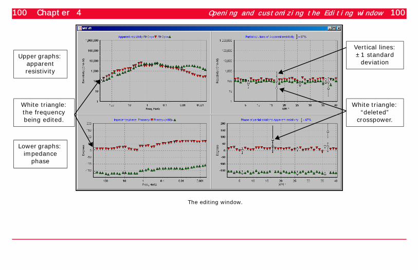
100 Chapter 4 Opening and customizing the Editing window 100
The editing window.
White triangle: the frequency being edited.
White triangle: “deleted”
crosspower.
Upper graphs: apparent resistivity
Lower graphs: impedance
phase
Vertical lines: ±1 standard
deviation

101 Chapter 4 Editing the crosspowers 101
Changing graph properties
The properties of the four graphs in the Editing window can be changed in the same way as those in the Starting data and Resulting data windows. See “Changing graph properties” on page 97 for instructions.
To change the proportions of the four graphs:
1. Position the mouse pointer on either the vertical or horizontal double lines that separate the graphs, until the pointer changes to a double-headed arrow.
2. Drag the double lines to a new position.
Tip On computers with small screens, it can be hard to position the editing cursor exactly on the crosspower you want to edit—especially if the number of crosspowers is large. Be sure to use the options of zooming and resizing the graphs and/or resizing the markers so you can work more easily.
Editing the crosspowersThe primary objective of editing is to create a smooth apparent resistivity curve, by eliminating from the calculation of each data point any crosspowers that were affected by noise. The editing is done by deleting or restoring individual crosspowers in the two graphs on the right of the window. The effect can be seen in the two graphs on the left of the window.
There are two methods of editing, auto and manual, as mentioned above. With normal quality data (low to moderate noise), it is best to start with autoediting and then refine the result with manual editing. With very noisy data, it may be faster to start by deleting all the crosspowers for a given frequency, and then selectively restore the best.
Tip Impedance phase is often more sensitive to noise than apparent resistivity is. You may find it most efficient to start editing using the phase graphs, then refine the result using the apparent resistivity graphs. For the best results, repeat the editing using different reference processing (Local E, Local H, etc.), if it is available.

102 Chapter 4 Editing the crosspowers 102
For efficency, scan the crosspowers for each frequency as you begin to edit them, and choose the most appropriate tool from the Cursors toolbar to make your changes.
• If only one or two crosspowers are of low quality, choose the Hand tool.
• If several crosspowers in a row are of low quality, edit them as a group. Choose the Two Vertical Lines or the Lasso tool and toggle its effect by choosing Deleting or Restoring from the Editmode toolbar.
To learn how to use all the tools, see “The Toolbars” on page 84.
To Autoedit the crosspowers:
• Click on the Processing toolbar.
To manually edit the crosspowers:
1. If necessary, click to make the first frequency active.
2. Evaluate the crosspowers in the right hand pane, looking for long vertical error bars (indicating a large standard deviation) and crosspowers that vary significantly from the others.
3. If it is helpful, show the Mean and/or Standard
Deviations of the crosspowers by clicking or
on the Show toolbar.
4. Use one of the tools on the Cursors toolbar to delete the low quality crosspowers (or to restore them if you change your mind).
5. Evaluate the effect of your editing by examining the left hand panes.
6. When you are satisfied with the results, move to the next crosspower (see “The Navigate toolbar” on page 86) and repeat from step 2.
7. When all the crosspowers from a given type of processing have been edited, consider whether the results can still be improved: if possible, select a different type of processing from the Reference
toolbar and repeat the editing process.

103 Chapter 4 Viewing the data mask 103
Viewing the data maskAlthough the terms Deleting and Restoring are used to refer to the editing process, no crosspowers are actually deleted from the data. Instead, they are temporarily removed from the calculations of the data points. It can be useful to have an overall view of how many crosspowers remain in use; the Mask View shows this information.
To view the data mask:
• Click on the View toolbar.
The Mask View window appears:

104 Chapter 4 Viewing the data mask 104
The Mask View window.
Each row of the Mask View table represents a single frequency, with high frequencies at the top of the table
and low frequencies at the bottom. Each cell in a row represents a single crosspower. White cells indicate
Light blue: included
crosspowers.
White: no data
Dark blue: “deleted”
crosspowers

105 Chapter 4 Viewing polar diagrams 105
there is no data; dark blue cells indicate “deleted” crosspowers; light blue cells indicate crosspowers that are included in the calculations.
Viewing polar diagramsPolar diagrams of the frequencies in your data set are available from the View menu and toolbar. Initially, a separate diagram will be created for each frequency, making the individual plots very small. However, it is easy to change the number of plots that are shown at one time, and to view only a subset of the data.
To view polar diagrams:
• Click on the View toolbar.
The Polar diagrams window opens.
Customizing the polar diagrams window
Use the controls on the right hand side of the polar diagrams window to customize the display.

106 Chapter 4 Printing 106
• Select or clear the components (Zxy, Zxx) that you want to display or hide. A checkmark indicates that a component is currently displayed.
• To see a contiguous subset of the data, choose from the drop-down lists the First and Last frequencies you want to view. (This is a good way to increase the size of individual plots.)
Note The value you set for First freq must be greater than the value for Last freq.
• To see a non-contiguous subset of the data, change the Step value. A Step value of 2 will display every second frequency between First and Last; a Step value of 3 will display every third frequency, and so on. (Increasing the Step value is also a good way to increase the size of the plots.)
• To normalize either of the component values, select the appropriate Normalize controls. A checkmark indicates that a component is currently normalized.
PrintingThe Print command on the Files menu is under development. At present, only some graphs can be Previewed or Printed from this menu, in portrait orientation only (regardless of print setup properties).
For more control over the appearance of a printed graph, use the following procedure.
To print a graph:
1. Right click on the graph and choose ChartEditor from the popup menu; if ChartEditor is not on the menu, choose Properties.
2. Click the Print tab.
3. Select the page orientation desired.
4. To change the margins, drag the dotted lines in the preview pane.
5. Click Setup to choose your printer and set its properties in a standard Windows Print Setup dialog.
6. Close the Print Setup dialog.

107 Chapter 4 Saving your work 107
7. Click Print.
Tip Most printing will be done from the Resulting data window, where the control areas make clear what components the markers represent. However, the control areas are not printed. To produce a meaningful printout, select Show legend before printing.
Saving your workYou should save your editing periodically as you work, before you close the file(s) you are editing, and before you exit the program.
To save your edits:
• On the Files toolbar, click either to save the file
with its current name, or to open the Save As dialog and save the file with a new name.
Exporting in EDI formatWhen you are satisfied with your edits, save the data for use with your interpretation software.
To export in EDI format:
1. Ensure that you have correctly set up the file header and format parameters using the Options command (see “Setting up export options” on page 88).
2. Click on the Files toolbar.
3. Navigate to the folder where you want to save the output file.
4. Choose the file format from the Save as type: drop-down list.
5. If desired, change the File name.
6. Click Save.
108 Chapter 4 Exporting in EDI format 108
109 Chapter 5 109
Chapter
Viewing Time Series Data withSynchro Time Series View
This chapter explains how to use Synchro Time Series View to view and print graphical representations of:• raw time series data.• power spectra derived from the time series data.• coherencies between pairs of channels.
The time series files must have been acquired with Phoenix System 2000 or System 2000.net equipment. Up to six channels from one or more files can be analysed at one time.

110 Exploring Synchro Time Series View 110
Exploring Synchro Time Series ViewStart Synchro Time Series View as you would any other Windows program: either double click a desktop shortcut, or launch the program from the Start menu.
Understanding the main window
When you launch the Synchro Time Series View program, the main application window appears (see the illustration on page 111).
Across the top of the main window are the Menus:
Below them is the Toolbar:
The Menus and the Toolbar both allow you to perform the most common tasks.
Across the bottom of the main window is the Status bar. At startup the bar is blank, but when time series channels are loaded, the Status bar displays information about the them.

111 Exploring Synchro Time Series View 111
The Synchro Time Series View main window.
Menu bar
Toolbar
Status bar

112 Viewing time series channels 112
Viewing time series channelsSynchro Time Series View can display and analyse up to six data channels at a time. The channels can be taken from more than one site, but the program will display only those records that lie within a common time span.
Opening time series files
The first task is to identify which channel(s) from which site(s) to load. Synchro Time Series View will automatically select the highest sampling rate from the first site you select, but you can easily choose another sampling rate if you want.
To load time series channels:
1. On the Toolbar, click or choose Open from the File menu.
The Load Time Series dialog box appears. Only the first Window button is enabled.
2. In the Window column, click .

113 Viewing time series channels 113
The Select TS File and Component dialog box appears.
3. Click and open any time series file (TSL, TSH, or TS2 to TS5) from the site you want to use.
4. In the Component area, click the channel you want to view.
5. Click OK to return to the Load Time Series dialog box.
The dialog box displays the names of the time series file and component, and the highest sampling rate of the site. The Window button for the next channel is enabled.
6. If you want to load all the remaining channels from
the chosen site, click . Otherwise, click
and load the next channel in the same manner as the first channel.
7. Continue by clicking the next numbered button until all desired channels are loaded.
Note: To load the same channels from other time series files from the same site(s), select a different sampling rate from any list in the Sampling column.
8. Click OK to return to the main window.

114 Viewing time series channels 114
The main window now displays the selected channels in graphical format. The Status bar displays the file name, record
number, saturation status, date, and channel of whichever time series record the mouse points to.

115 Viewing time series channels 115
Note: The program opens in a maximized window. If you resize the window, it may become too small to show the Status bar. Increase the size of the window slightly to bring the Status bar back into view.
Specifying start and end times
Time series files can be very large, depending on the sampling schedule and the length of acquisition. You may want to view only a subset of the records in your files. You can specify start and end times other than the beginning and end of a file.
To specify start and end times:
1. From the Options menu, choose TS info options…
The Time Series Info Options dialog box appears:
2. Select Specify start/end time for loading.
3. Click OK.
4. From the File menu, choose Open and load the files you want to view, as described earlier in this chapter.
When you click OK in the final step of loading, the Specifying Times dialog box appears:

116 Viewing time series channels 116
5. Edit the dates and/or times displayed in the dialog box and click OK.
The channels are loaded and displayed in the main window.
Troubleshooting time series files
This section describes a method of opening files that otherwise fail to open and cause an error in Synchro Time Series View.
When you open time series files, Synchro Time Series View reads the associated site parameter (TBL) file to get information on start and end times, number of records, etc. Sometimes (especially with files from
instruments with older firmware) there may be problems getting all the required information from the site parameter file alone.
If you experience problems opening files, it may help to have the program read and analyse the time series files directly to get the required information. (Files may take slightly longer to load if you select this option.)
To open files by analysing the time series records:
1. From the Options menu, choose TS info options…
The Time Series Info Options dialog box appears:

117 Modifying the time series view 117
2. Click Analyse TS files.
3. Click OK.
4. Try again to open the file(s) that caused problems.
If you still cannot open the files, contact Phoenix for support.
Modifying the time series viewSynchro Time Series View provides several controls for modifying the time series view. You can scroll through the records, change the number of scans shown in the window, and change the vertical scale of each chart.
The default scale normalizes the data to use the full height of each strip chart with zero in the centre (called “Adaptive scale”) and DC offset automatically corrected. Adaptive scale applies to all the scans visible in a given window. When the signal amplitude varies as you scroll through the data, the vertical scale will grow or shrink as needed to normalize the scans currently visible.
You can disable adaptive scaling and increase or decrease the limits manually. You can also disable the DC offset autocorrection. Either of these changes may require you to shift the y-axis origin up or down in order to see the data.
To change the number of scans visible:• On the Toolbar, select the desired number of scans in
the Scans per window list. (The choices will vary depending on the frequency band of the time series files.)
To scroll through all the records sequentially:
• Click or on the Toolbar.

118 Modifying the time series view 118
To scroll by increments of 1% of the file length:• Click the scroll arrows at either end of the scroll bar
or press the LEFT ARROW or RIGHT ARROW keys.
To scroll by increments of 10% of the file length:• Click in the scroll bar on either side of the scroll box.
To scroll rapidly:• Drag the scroll box. (The smallest increment with this
method is 1% of the file length.)
To change the vertical scale or shift the y-axis origin:
1. Right-click on the chart of the channel you want to
change (or click on the Toolbar, or choose Vertical Scales from the View menu).
The Scale Settings dialog box appears.
2. Clear the Adaptive scale check box.
3. Enter a new maximum value for the vertical scale of any channel. (The value is multiplied by –1 to set the minimum value.)

119 Viewing power spectra 119
4. If you want to change the position of the y-axis origin, click one of the Shift scope buttons.
The y-axis origin will be moved a distance equal to half the original Maximum value.
5. Click OK to return to the main window.
To restore the vertical scale:
1. Right-click on the chart of the channel you want to change.
• To restore the original maximum and minimum and move the y-axis origin back to the centre of
the chart, click
• to restore adaptive scaling, select Adaptive scale
• to remove DC offset effects, select DC offset auto correction
2. Click OK to return to the main window.
Viewing power spectraSynchro Time Series View includes the capability of calculating power spectra, as well as coherency between pairs of channels.
To calculate and view power spectra:
1. Load the time series files that you want to work with.
2. On the Toolbar, click , or choose Compute Spectra from the Spectra menu.

120 Viewing power spectra 120
The Spectra Computation dialog box appears.
3. Choose the number of samples for each Fourier Transform calculation. (The choices will vary depending on the frequency band of the time series files; lower numbers will produce smoother curves.)
4. Choose the algorithm to be used in the Data window (Hann, Nuttall, or Rectangular).
5. Optionally, to prevent saturated records from being included in the calculations, select Skip saturated records.
6. Click OK.
A progress dialog box appears while the program computes the power spectra, and then the Spectra window appears, maximized. If both E and H channels have been analysed, the window will be split; if only one type of channel has been analysed, the curves will fill the window.
Note: If Skip saturated records is selected and the time series files contain many saturations, there may not be enough valid records to compute the spectra. Synchro Time Series View will display the error message, “No acceptable time segments found.”

121 Viewing power spectra 121
The Spectra window.
E channels
H channels
Spectra legend
Scale legends

122 Modifying the spectra view 122
Modifying the spectra viewThe Spectra window provides several controls for modifying the view. You can choose which channel(s) to plot, change the scales, enlarge a portion of the curves, and pinpoint values on the curves.
To select channels for plotting:
1. The curves are colour-coded in the Spectra legend; clear the check box of any channel you want to remove from the graph.
2. To restore a curve to the graph, select it in the Spectra legend.
By default, the graph is plotted on a logarithmic scale for both axes, with frequency on the x-axis.
To change the frequency scale:• Choose Log or Linear from the Freq. Scale legend.
By default, the curves are scaled to fill the available space. You can override this setting by changing the scale of either x or y axis, or both.
To change the axes limits:
1. In the Scale legend, clear the Auto check box.
2. Click .
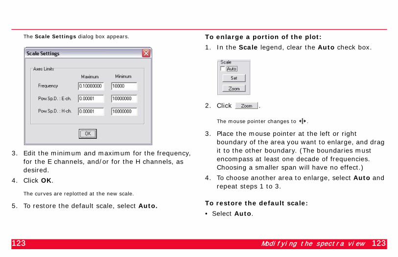
123 Modifying the spectra view 123
The Scale Settings dialog box appears.
3. Edit the minimum and maximum for the frequency, for the E channels, and/or for the H channels, as desired.
4. Click OK.
The curves are replotted at the new scale.
5. To restore the default scale, select Auto.
To enlarge a portion of the plot:
1. In the Scale legend, clear the Auto check box.
2. Click .
The mouse pointer changes to .
3. Place the mouse pointer at the left or right boundary of the area you want to enlarge, and drag it to the other boundary. (The boundaries must encompass at least one decade of frequencies. Choosing a smaller span will have no effect.)
4. To choose another area to enlarge, select Auto and repeat steps 1 to 3.
To restore the default scale:
• Select Auto.

124 Viewing coherencies 124
To pinpoint values on the curves:• Position the mouse pointer over a point on the curve
and read the frequency and power spectra density (PSD) values below the Scale legends, between the Coh and Print buttons.
Viewing coherenciesOnce the power spectra have been calculated, it’s easy to plot the coherencies between all the pairs of channels.
To view coherencies:
1. From the Spectra window, click .
The Coherencies window appears, showing curves for all possible channel pairs.
2. The curves are colour-coded in the Component Pairs legend; clear the check box of any channel you want to remove from the graph.
3. To restore a curve to the graph, select it in the Component Pairs legend.

125 Printing time series, spectra, and coherency plots 125
To pinpoint values on the curves:• Position the mouse pointer over a point on the curve
and read the frequency and coherency values below the Component Pairs legend.
4. To return to the Spectra window, close the Coher-encies window.
Printing time series, spectra, and coherency plotsAny of the plots can be printed to any printer connected to your PC.
To print the plots:
1. For time series, click on the Toolbar or choose Print from the File menu.
For spectra or coherencies, click .
The Print Preview window appears.
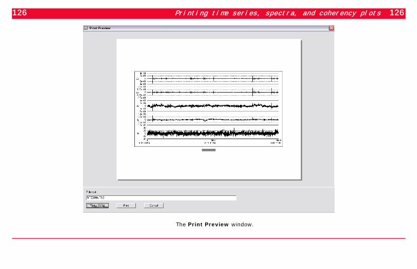
126 Printing time series, spectra, and coherency plots 126
The Print Preview window.

127 Printing time series, spectra, and coherency plots 127
2. Edit the Title text, which will appear on the print-out centred below the plot.
3. If you want to modify the default printer settings (choice of printer, page orientation, margins, etc.),
click .
A standard Windows printer setup dialog box appears.
4. Set up the printer as desired and click OK.
5. Click to send the plot to the printer, or
click to return to the plot without printing.
128 Printing time series, spectra, and coherency plots 128

129 Appendix A 129
Appendix
Data processing flowchart
The chart on the following pages illustrates the steps required to process data. The chart shows the source, the method used, and the result for each step.

ACTION SOURCE METHOD RESULT
BEFORE DATA ACQUISITION
Copy calibration files to PC
1 CAL
*.CLC*.CLB
TAG-TSer
TAG-CAL
Verify calibrations
2 TAG-TSer
TAG-CAL*.CLC*.CLB
AFTER DATA ACQUISITION
Copy data files to PC
3 DATA
*.TBL*.TSn
TAG-TSer
AMT
yyyy-Hdd
MT
yyyy-Hdd
UMT
yyyy-Hdd
Verify & edit site parameters
4 yyyy-Hdd*.TBL
yyyy-Hdd*.TBL (edited)*.TBO (original)
Optional: View TBL file
4a
yyyy-Hdd*.TBL
Archive data
5 yyyy-Hdd CD or DVD burning software, or
copy to ZIP drive
or
Set up Fourier Transform
parameter file for the project
6 yyyy-Hdd*.TBL
SSMT-PFTMA35DN4D.PFTMM55DN4D.PFTMU55DN4D.PFT...Project.PFT
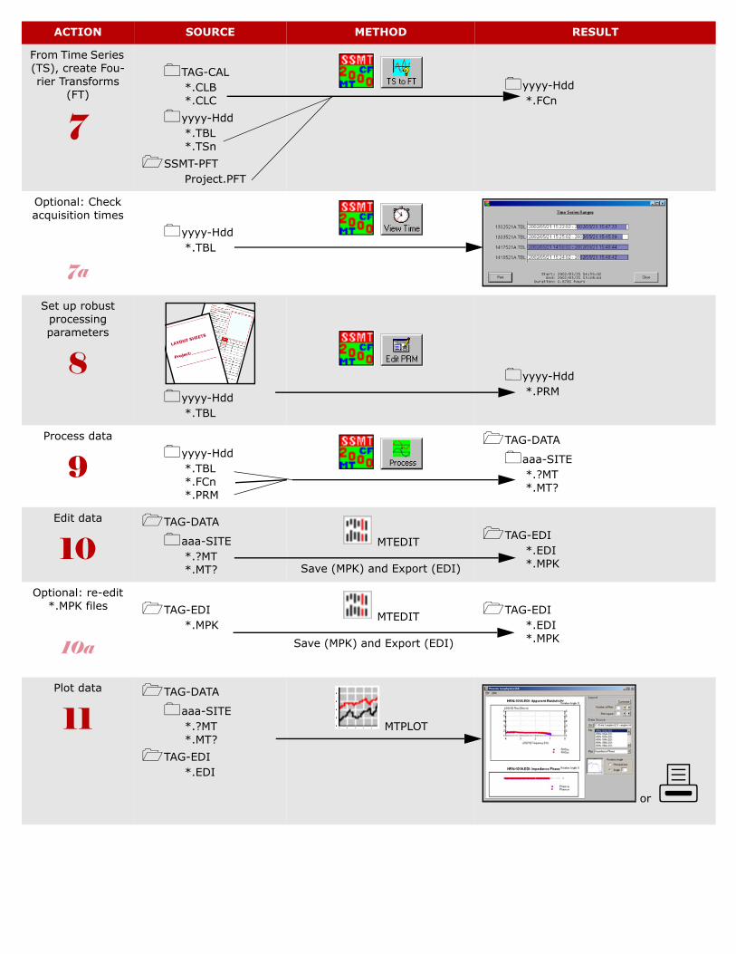
From Time Series (TS), create Fou-rier Transforms
(FT)
7
TAG-CAL*.CLB*.CLC
yyyy-Hdd*.TBL*.TSn
SSMT-PFTProject.PFT
yyyy-Hdd*.FCn
Optional: Check acquisition times
7a
yyyy-Hdd*.TBL
Set up robust processing parameters
8 yyyy-Hdd*.TBL
yyyy-Hdd*.PRM
Process data
9 yyyy-Hdd*.TBL*.FCn*.PRM
TAG-DATA
aaa-SITE*.?MT*.MT?
Edit data
10 TAG-DATA
aaa-SITE*.?MT*.MT?
MTEDIT
Save (MPK) and Export (EDI)
TAG-EDI*.EDI *.MPK
Optional: re-edit *.MPK files
10a
TAG-EDI*.MPK
MTEDIT
Save (MPK) and Export (EDI)
TAG-EDI*.EDI *.MPK
Plot data
11 TAG-DATA
aaa-SITE*.?MT*.MT?
TAG-EDI*.EDI
MTPLOT
or
ACTION SOURCE METHOD RESULT

131 Appendix B 131
Appendix
Installing software and setting upyour PC
Before processing data for the first time, you must install the Phoenix processing software on your computer and prepare your file system. This appendix tells you how.

132 Appendix B System requirements 132
System requirementsPhoenix software is designed to run on a PC equipped with:
• Microsoft® Windows™ 95, 98, Me, or XP• Pentium processor• 100MB of free space on drive C: (for applications)• 500MB of additional free space on any drive (for
temporary files created during processing)• CD-ROM or CD-RW drive for loading software• CD-RW, DVD-RW, or other mass storage drive for
archiving data• super VGA (800 x 600) or higher resolution monitor• parallel port configured as ECP (See “Configuring the
parallel port” on page 134.)• keyboard and mouse or other pointing device• Internet access (optional, for software updates)
Note Data processing can be very time-consuming on older computers. Phoenix recommends using a recent vintage, high-speed Pentium processor. (Celeron processors are not recommended)
Installing the softwarePhoenix software is shipped on a CD-ROM that also contains sample data. The data folder is not copied to the PC during the installation process, but can be copied manually if desired.
The Setup program will install MTU and MTU-A Host software, SSMT2000 data processing software, and MT-Plot software. Overall installation is controlled by a batch file that requires you to press a key to start each of the phases of installation.
To install the software:
1. If Phoenix software has already been installed on your PC, change the name of the folder C:\EMT-SW to preserve your previous work.
2. Close any applications that are currently running.
3. Insert the Phoenix CD into the CD-ROM drive.
4. If Autorun is enabled, wait for Windows Explorer to open. If Windows Explorer does not open automatically, double click on the CD-ROM icon on the desktop.

133 Appendix B Installing the software 133
5. Double click on Setup.Bat and follow the instruc-tions on screen.
6. Be sure to return to the Setup batch window (a DOS window) and press any key to start each subsequent phase of installation.
Installation is complete when the Setup batch window title says “Finished.”
After installing the software, follow the instructions on page 134 to configure the parallel port.
Note Some customers have reported problems installing the software on Windows Me systems. If your installation fails, use the following alternate procedure.
To install the software (alternate for Windows Me):
1. If Phoenix software has already been installed on your PC, change the name of the folder C:\EMT-SW to preserve your previous work.
2. Close any applications that are currently running.
3. Create a new temporary folder on your desktop, called PGL.
4. Insert the Phoenix CD into the CD-ROM drive.
5. If Autorun is enabled, wait for Windows Explorer to open. If Windows Explorer does not open automatically, double click on the CD-ROM icon on the desktop.
6. Copy these folders from the CD to the PGL folder you created:
• 1_PC HOST FILES
• 2_PROGRAMS
• 3_SSMT2000
7. Copy these files from the CD to the PGL folder you created:
• autorun.inf
• ReadMe.html
• Setup.Bat
8. In the PGL folder, double click Setup.Bat and follow the instructions on screen.
9. Be sure to return to the Setup batch window (a DOS window) and press any key to start each subsequent phase of installation.

134 Appendix B Configuring the parallel port 134
Installation is complete when the Setup batch window title says “Finished.”
After installing the software, follow the next procedure to configure the parallel port.
Configuring the parallel portThe WinHost program communicates with an MTU⁄MTU-A via a special cable (part number 6218) and adapter (part number 6228) connected to the PC’s parallel port.
The parallel port must be configured as an Extended Capability Port (ECP). ECP provides a high-performance bi-directional communication path between the PC and the instrument. Your PC may already be configured to use the ECP protocol, in which case you need to verify the setup only if you experience problems using WinHost. Otherwise, you will have to configure the port in your computer’s CMOS Setup.
To determine the parallel port configuration:
1. Right-click on My Computer and choose Properties.
2. If your operating system is Windows Me or earlier, click the Device Manager tab; if your operating system is Windows XP, click the Hardware tab and then the Device Manager button.
3. Expand the Ports (COM & LPT) entry by clicking the plus sign to the left of it. (See the illustration on page 135.)
4. If there is an ECP Printer Port listed, verify the ECP port Properties as described on page 136. If there is no ECP Printer Port listed, follow the next procedure to create the port.

135 Appendix B Configuring the parallel port 135
To create an ECP parallel port:
1. Be prepared to issue the keyboard command that puts your PC into CMOS Setup during system startup (“cold boot”). This command varies from one manufacturer and model to another. Consult
your PC documentation or the manufacturer’s Web site. (Typically, the command key is one of the Function keys or the Insert or Delete key. Many computers, when they are powered on, will display a prompt that names the command key.)
2. Follow the instructions just given to determine the parallel port configuration. If there is an SPP Standard Parallel Port listed, select it and click Remove. Close the Properties dialog box.
3. Restart your computer. (You may have to shut down your computer completely before restarting it in order to reach the CMOS Setup prompt.)
4. During the restart, before the Windows logo screen appears, type the keyboard command to enter CMOS Setup.
5. Consult your PC documentation or follow the on-screen prompts for instructions, and change the parallel port to ECP. If there are options for a DMA channel or Interrupt Request, accept the defaults.
6. Save the new settings and exit CMOS Setup.
7. Allow Windows to continue loading, and observe whether it detects and configures the new ECP port.
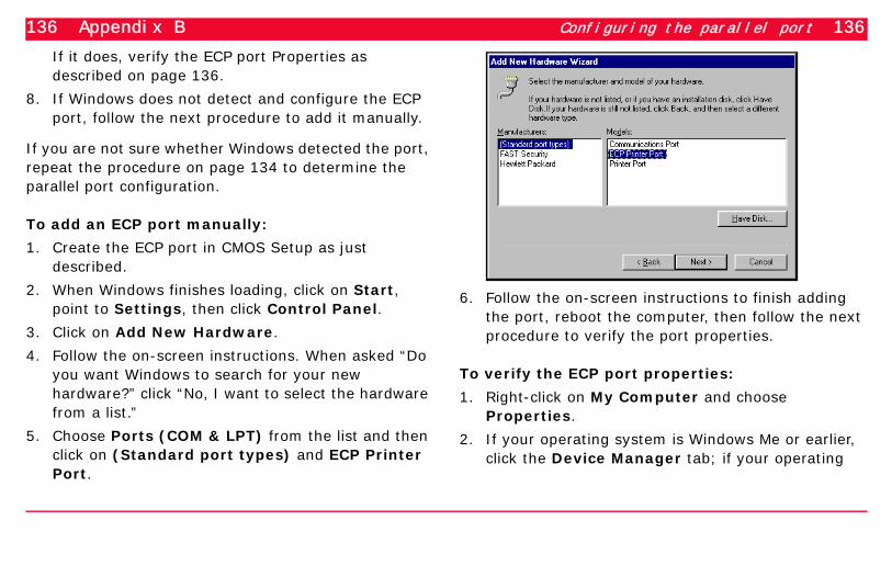
136 Appendix B Configuring the parallel port 136
If it does, verify the ECP port Properties as described on page 136.
8. If Windows does not detect and configure the ECP port, follow the next procedure to add it manually.
If you are not sure whether Windows detected the port, repeat the procedure on page 134 to determine the parallel port configuration.
To add an ECP port manually:
1. Create the ECP port in CMOS Setup as just described.
2. When Windows finishes loading, click on Start, point to Settings, then click Control Panel.
3. Click on Add New Hardware.
4. Follow the on-screen instructions. When asked “Do you want Windows to search for your new hardware?” click “No, I want to select the hardware from a list.”
5. Choose Ports (COM & LPT) from the list and then click on (Standard port types) and ECP Printer Port.
6. Follow the on-screen instructions to finish adding the port, reboot the computer, then follow the next procedure to verify the port properties.
To verify the ECP port properties:
1. Right-click on My Computer and choose Properties.
2. If your operating system is Windows Me or earlier, click the Device Manager tab; if your operating
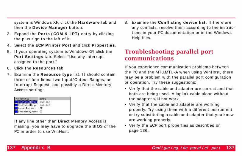
137 Appendix B Configuring the parallel port 137
system is Windows XP, click the Hardware tab and then the Device Manager button.
3. Expand the Ports (COM & LPT) entry by clicking the plus sign to the left of it.
4. Select the ECP Printer Port and click Properties.
5. If your operating system is Windows XP, click the Port Settings tab. Select “Use any interrupt assigned to the port.”
6. Click the Resources tab.
7. Examine the Resource type list. It should contain three or four lines: two Input/Output Ranges, an Interrupt Request, and possibly a Direct Memory Access setting:
If any line other than Direct Memory Access is missing, you may have to upgrade the BIOS of the PC in order to use WinHost.
8. Examine the Conflicting device list. If there are any conflicts, resolve them according to the instruc-tions in your PC documentation or in the Windows Help files.
Troubleshooting parallel port communications
If you experience communication problems between the PC and the MTU⁄MTU-A when using WinHost, there may be a problem with the parallel port configuration or operation. Try these suggestions:
• Verify that the cable and adapter are correct and that both are being used. A laplink cable alone without the adapter will not work.
• Verify that the cable and adapter are working properly. Try using them with a different instrument, or try substituting a cable and adapter that you know are working properly.
• Verify the ECP port properties as described on page 136.

138 Appendix B Updating the software 138
• Verify that the parallel port is working properly by connecting a printer (using a standard printer cable) and printing a test document.
• If your operating system is Windows XP and you receive error code 54, “ECP driver is not set up to use an interrupt,” verify that the Port Settings will “Use any interrupt assigned to the port.” (See step 5 on page 137.)
• If you receive error code 4096, “Error setting up timer event,” Windows is out of memory. Reboot the PC.
• If you receive error code 4098, “ECR register not detected,” the system BIOS is not set for ECP mode. Follow the instructions under “Configuring the parallel port” on page 134, being sure to save the settings when exiting CMOS setup.
• If you receive error code 4097, “Error accessing the driver,” Windows XP is attempting to run WinHost in “compatibility” mode. Follow the next procedure to change the mode.
To disable “compatibility” mode in Windows XP:
1. From the Start menu, click Programs, point to Phoenix Geophysics Host Software, and right-click on WinHost.
2. Click Properties.
3. Click the Compatibility tab.
4. Clear the Compatibility mode checkbox.
5. Click OK.
Updating the softwarePeriodic updates to SSMT2000 processing software are made available through the Phoenix website. SSMT2000 includes a utility to check for and install updates.
To check for updates:
1. Ensure that your computer is connected to the Internet.
2. Launch SSMT2000.

139 Appendix B Registering MT-Editor 139
3. From the Help menu, choose Check for Updates.
A Warning dialog appears.
4. Click Yes to continue.
SSMT2000 closes temporarily, determines current software versions, and checks for updates.
A DOS-mode screen appears briefly during this process.
5. If updates are available, follow the instructions on screen to complete the updating process.
Registering MT-EditorAfter installation, the MT-Editor program must be registered (by e-mail to Phoenix) in order to enable the saving and exporting functions. Up to three copies of MT-Editor can be registered for each purchased license.
To request an MT-Editor Serial Number:
1. After installing the software, launch MT-Editor.
2. From the MT-Editor Help menu, choose Regis-tration.
3. Select the text in the Hardware ID box and press CTRL+C to copy the text to the clipboard.
4. Close the dialog box and exit from MT-Editor.
5. Launch your e-mail client and create a new message to:[email protected]
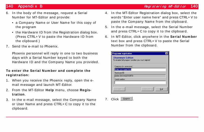
140 Appendix B Registering MT-Editor 140
6. In the body of the message, request a Serial Number for MT-Editor and provide:
• a Company Name or User Name for this copy of the program
• the Hardware ID from the Registration dialog box. (Press CTRL+V to paste the Hardware ID from the clipboard.)
7. Send the e-mail to Phoenix.
Phoenix personnel will reply in one to two business days with a Serial Number keyed to both the Hardware ID and the Company Name you provided.
To enter the Serial Number and complete the registration:
1. When you receive the Phoenix reply, open the e-mail message and launch MT-Editor.
2. From the MT-Editor Help menu, choose Regis-tration.
3. In the e-mail message, select the Company Name or User Name and press CTRL+C to copy it to the clipboard.
4. In the MT-Editor Registration dialog box, select the words “Enter user name here” and press CTRL+V to paste the Company Name from the clipboard.
5. In the e-mail message, select the Serial Number and press CTRL+C to copy it to the clipboard.
6. In MT-Editor, click anywhere in the Serial Number text box and press CTRL+V to paste the Serial Number from the clipboard.
7. Click .

141 Appendix B Organizing your files 141
Organizing your filesPhoenix software relies on several file naming and organization conventions. Although it is possible to follow alternate plans, we strongly recommend that you establish the following file and folder conventions in order to minimize problems.
Note In all cases, limit folder and file names to eight characters, and file extensions to three characters. Do not use spaces in path names, file names, or extensions. Some language versions of Microsoft Windows (Russian, for example) will cause problems if file names consist only of digits. Ensure that the first character of a file name is an alphabetic character, not a digit.
For each survey you conduct, three types of files need to be stored and organized on your PC: calibration files, raw data (time series) files, and processed data (plot) files.
We recommend establishing a three-letter tag for each survey, and using that tag in the name of each folder containing files related to the survey.
For example, in a survey of Three River Valley, you might choose TRV as the tag. You would then create:
• a folder called TRV-TSER for the daily time series folders.
• within TRV-TSER, a folder called TRV-Cal for the calibration files.
• a folder called TRV-DATA for the plot file folders.
You would also use the TRV tag when naming sites in the Multi-table editor (see “Editing site parameters with the Multi-table Editor” on page 20.)
Storing raw data files
The raw data files are named by the MTU⁄MTU-A in the formats ssssHdda.TBL and ssssHdda.TS? where:
• “ssss” represents the serial number of the A/MTU.• “H” represents the month in hexadecimal.• “dd” represents the day of the month in decimal.
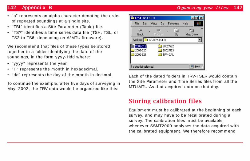
142 Appendix B Organizing your files 142
• “a” represents an alpha character denoting the order of repeated soundings at a single site.
• “TBL” identifies a Site Parameter (Table) file.• “TS?” identifies a time series data file (TSH, TSL, or
TS2 to TS6, depending on A/MTU firmware).
We recommend that files of these types be stored together in a folder identifying the date of the soundings, in the form yyyy-Hdd where:
• “yyyy” represents the year.• “H” represents the month in hexadecimal.• “dd” represents the day of the month in decimal.
To continue the example, after five days of surveying in May, 2002, the TRV data would be organized like this:
Each of the dated folders in TRV-TSER would contain the Site Parameter and Time Series files from all the MTU⁄MTU-As that acquired data on that day.
Storing calibration files
Equipment must be calibrated at the beginning of each survey, and may have to be recalibrated during a survey. The calibration files must be available whenever SSMT2000 analyses the data acquired with the calibrated equipment. We therefore recommend

143 Appendix B Formatting a CompactFlash card 143
storing the calibration files in a TAG-CAL folder within the TAG-TSER folder, as illustrated above. This distinguishes the calibration files from others created with the same equipment on other surveys, and also ensures that when the TAG-TSER folder is archived, the calibration files are included.
In the case where equipment must be recalibrated during a survey, the new files could be stored in folders called TAG-CAL1, TAG-CAL2, etc.
Storing output (plot) files
The data from survey sites may have to be processed several times using different parameters in order to get satisfactory results in all the desired frequency ranges. For this reason, we recommend creating a TAG-DATA folder and within it various aaa-SITE folders, where “aaa” is an abbreviation or code relating to the type of processing performed.
For example, if you processed Three River Valley site data using a remote magnetic (H) reference, you might store the output files in a folder called ReH-SITE. If you
used a local telluric (E) reference, the folder might be called LoE-SITE. You would store both these folders in a folder called TRV-DATA.
You can create the SITE folders in advance if you want, or simply create them as needed using the Magnetotelluric Processing Setup dialog. (The TAG-DATA folder that is to contain the SITE folders must be set up in advance, however.) See “Reprocessing the Fourier transforms” on page 29.
Formatting a CompactFlash cardCompactFlash cards must be correctly formatted before use.

144 Appendix B Formatting a CompactFlash card 144
Note The formatting utility provided by SanDisk corporation is not compatible with Phoenix instruments. CompactFlash cards must use the FAT or FAT16 (File Allocation Table) file system applied by the Windows formatting utility. Do not format as FAT32 or NTFS.If you experience operating system crashes when inserting a CompactFlash card into the reader, the problem may be caused by static electricity. Touch a grounded object such as an unpainted area of the computer case before inserting the card.
To format a CompactFlash card:
1. Insert the card into a card reader connected to the PC.
2. Double click My Computer.
3. Right-click the CompactFlash card drive letter and click Format…
4. If your operating system is Windows XP, be sure that the File system is set to FAT. (In earlier Windows versions, the file system is always FAT.)
5. If desired, type a volume label (a name for the disk).
6. If Quick Format is selected, clear the checkbox.
7. Click Start.
When formatting is complete, click Close. The card is ready for use in Phoenix instruments.

145 Appendix C 145
Appendix
Frequency tables for SSMT2000
This appendix provides charts of all the frequencies output by SSMT2000 for various combinations of:
• Line Frequency filter.• A/MTU box type.• Firmware version.• Sensor type.• Frequencies per octave.
The first half of the appendix covers the line frequency filter of 50Hz; the second half covers the line frequency filter of 60Hz. The tables appear in order from highest to lowest frequencies.

146
Appendix C
146 Table C-1: 50Hz LF, MTU-A, AMTC-30
SamplingRate, Hz
2 Frequencies/ octave, Hz
4 Frequencies/ octave, Hz
SamplingRate, Hz
Firmware: B B
Range Name:
EMT (50) EMT (50)
24000FC2
10666.67 10400 24000FC28800
8000 7200
6000
5333.33 5200
4400
4000 3600
3000
2666.67 2600
2200
2000 1800
1500
1333.33 1300
1100
1000 900
776.47 2400FC3666.67 635.29
529.41
500 458.82
388.235
Firmware: B B
Range Name:
EMT (50) continues
EMT (50) continues
Firmware: Ext. Range
Range Name:
LMT (50) begins
2400FC3
320 317.645
264.705
240 229.41
194.1175
160 158.8225
132.3525
120 114.705
97.0588
80 79.4113
66.1763

147
Appendix C
147
2400FC3
60 57.3525 2400FC348.5294
40 39.7056
32.5 150FC430 27.5
22.5
20 18.75
16.25
15 13.75
11.25
Firmware: B B
Range Name:
EMT (50) continues
EMT (50) ends
Firmware: Ext. Range
Range Name:
LMT (50) continues
2400FC3
10 9.375
8.125
7.5 6.875
5.625
150FC4
6 4.6875 150 (AMT)15 (MT)
FC54.0625
4.5 3.4375
2.8125
3 2.34375
2.03125
2.25 1.71875
1.40625
1.5 1.17188
1.01563
1.125 0.85938
0.70313
0.75 0.58594
0.50781
0.5625 0.42969
0.35156
Table C-1: 50Hz LF, MTU-A, AMTC-30(cont’d)
SamplingRate, Hz
2 Frequencies/ octave, Hz
4 Frequencies/ octave, Hz
SamplingRate, Hz

148
Appendix C
148
Shaded areas indicate overlap of frequency ranges.
150 (AMT)15 (MT)
FC5
0.375 0.2929688 150 (AMT)15 (MT)
FC60.2539063
0.28125 0.2148438
0.1757813
0.1875 0.1464844
0.1269532
0.140625 0.1074219
0.0878907
0.09375 0.0732422
0.0634766
0.070313 0.053711
0.0439453
0.046875 0.0366211
0.0317383
0.035156 0.0268555
0.0219727
0.023438 0.0183106
0.0158691
0.017578 0.0134277
0.0109863
Table C-1: 50Hz LF, MTU-A, AMTC-30(cont’d)
SamplingRate, Hz
2 Frequencies/ octave, Hz
4 Frequencies/ octave, Hz
SamplingRate, Hz

149
Appendix C
149

150
Appendix C
150 Table C-2: 50Hz LF, MTU-A, MTC-50
SamplingRate, Hz
2 Frequencies/ octave, Hz
4 Frequencies/ octave, Hz
SamplingRate, Hz
Firmware: Hi Range Hi Range
Range Name:
HMT (50) HMT (50)
2400FC3
320 317.645 2400FC3264.705
240 229.41
194.11765
160 158.8225
132.3525
120 114.705
97.05883
80 79.41125
66.17625
60 57.3525
48.52941
40 39.70563
32.5 150FC430 27.5
22.5
20 18.75
16.25
15 13.75
11.25
Firmware: Hi Range Hi Range
Range Name:
HMT (50) continues
HMT (50) continues
Firmware: Lo Range
Range Name:
RMT (50) begins
2400FC3
10 9.375
8.125
7.5 6.875
5.625
150FC4
6.0 4.6875 150 (AMT)15 (MT)
FC54.0625
4.5 3.4375
2.8125
3.0 2.34375
2.03125

151
Appendix C
151
150FC4
2.25 1.71875 150 (AMT)15 (MT)
FC51.40625
1.5 1.171875
1.015625
1.125 0.859375
0.703125
0.75 0.5859375
0.5078125
0.5625 0.4296875
0.3515625
Firmware: Hi, Lo Ranges Hi Range
Range Name:
HMT (50), RMT (50) continue
HMT (50) ends
Firmware: Lo Range
Range Name:
RMT (50) begins
150 (AMT)15 (MT)
FC5
0.375 0.2929688 150 (AMT)15 (MT)
FC60.2539063
0.28125 0.2148438
0.1757813
0.1875 0.1464844
0.1269532
0.140625 0.1074219
0.0878907
0.09375 0.0732422
0.0634766
0.070313 0.053711
0.0439453
0.046875 0.0366211
0.0317383
0.035156 0.0268555
0.0219727
0.023438 0.0183106
0.0158691
0.017578 0.0134277
0.0109863
Table C-2: 50Hz LF, MTU-A, MTC-50 (cont’d)
SamplingRate, Hz
2 Frequencies/ octave, Hz
4 Frequencies/ octave, Hz
SamplingRate, Hz

152
Appendix C
152
Firmware: Hi Range Lo Range
Range Name:
HMT (50) continues
RMT (50) continues
Firmware: Ext. Range
Range Name:
LMT (50) begins
150 (AMT)15 (MT)
FC6
0.011719 0.009155275 150 (AMT)15 (MT)
FC70.007934572
0.0087891 0.006713869
0.005493166
0.0058594 0.0045776
0.0039673
0.0043945 0.0033569
0.0027466
0.0029297 0.0022888
0.0019836
0.0021973 0.0016785
0.0013733
0.0014648 0.0011444
0.0009918
0.0010986 0.0008392
0.0006866
0.0007324 0.0005722
0.0004959
0.0005493 0.0004196
0.0003433
Firmware: Hi Range Lo Range
Range Name:
HMT (50) ends RMT (50) ends
Firmware: Lo Range Ext. Range
Range Name:
RMT (50) continues
LMT (50) continues
150 (AMT)15 (MT)
FC7
0.0003662 0.0002861 150 (AMT)15 (MT)
FC80.000248
0.0002747 0.0002098
0.0001717
0.0001831 0.0001431
0.000124
Table C-2: 50Hz LF, MTU-A, MTC-50 (cont’d)
SamplingRate, Hz
2 Frequencies/ octave, Hz
4 Frequencies/ octave, Hz
SamplingRate, Hz
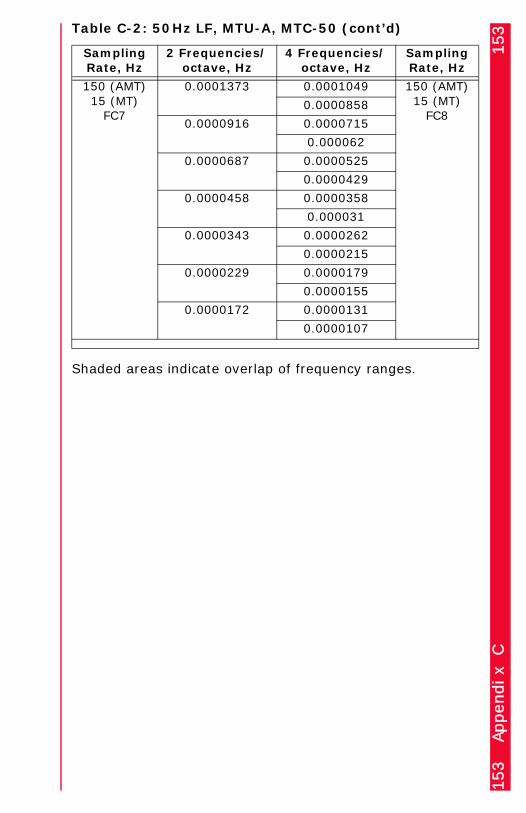
153
Appendix C
153
Shaded areas indicate overlap of frequency ranges.
150 (AMT)15 (MT)
FC7
0.0001373 0.0001049 150 (AMT)15 (MT)
FC80.0000858
0.0000916 0.0000715
0.000062
0.0000687 0.0000525
0.0000429
0.0000458 0.0000358
0.000031
0.0000343 0.0000262
0.0000215
0.0000229 0.0000179
0.0000155
0.0000172 0.0000131
0.0000107
Table C-2: 50Hz LF, MTU-A, MTC-50 (cont’d)
SamplingRate, Hz
2 Frequencies/ octave, Hz
4 Frequencies/ octave, Hz
SamplingRate, Hz

154
Appendix C
154 Table C-3: 50Hz LF, MTU, AMTC-30 (V5-comp.)
SamplingRate, Hz
2 Frequencies/ octave, Hz
4 Frequencies/ octave, Hz
SamplingRate, Hz
Firmware: Up Range Up Range
Range Name:
EMT (50) EMT (50)
2560FC3
640 720 2560FC3600
480 520
440
320 360
300
240 260
220
160 180
150
120 130
110
80 90
75
60 65
55
320FC4
40 45
37.5 320FC430 32.5
27.5
20 22.5
18.75
15 16.25
13.75
10 11.25
9.375
7.5 8.125
6.875
24FC5
6 5.625
4.875 24FC54.5 4.125
3.375
3 2.8125
2.4375

155
Appendix C
155
24FC5
2.25 2.0625 24FC51.6875
1.5 1.40625
1.21875
1.125 1.03125
0.84375
0.75
0.5625
0.375
0.2813
Table C-3: 50Hz LF, MTU, AMTC-30 (V5-
SamplingRate, Hz
2 Frequencies/ octave, Hz
4 Frequencies/ octave, Hz
SamplingRate, Hz
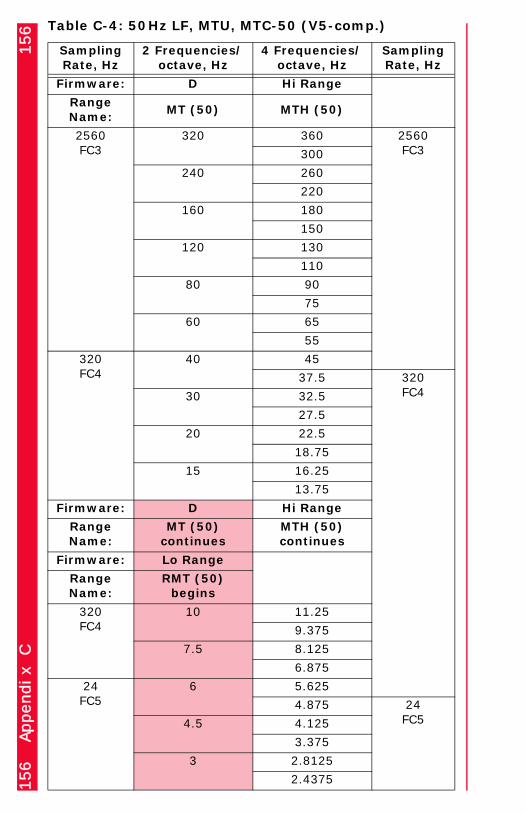
156
Appendix C
156 Table C-4: 50Hz LF, MTU, MTC-50 (V5-comp.)
SamplingRate, Hz
2 Frequencies/ octave, Hz
4 Frequencies/ octave, Hz
SamplingRate, Hz
Firmware: D Hi Range
Range Name:
MT (50) MTH (50)
2560FC3
320 360 2560FC3300
240 260
220
160 180
150
120 130
110
80 90
75
60 65
55
320FC4
40 45
37.5 320FC430 32.5
27.5
20 22.5
18.75
15 16.25
13.75
Firmware: D Hi Range
Range Name:
MT (50) continues
MTH (50) continues
Firmware: Lo Range
Range Name:
RMT (50) begins
320FC4
10 11.25
9.375
7.5 8.125
6.875
24FC5
6 5.625
4.875 24FC54.5 4.125
3.375
3 2.8125
2.4375

157
Appendix C
157
24FC5
2.25 2.0625 24FC51.6875
1.5 1.40625
1.21875
1.125 1.03125
0.84375
0.75 0.70313
0.60938
0.5625 0.51563
0.42188
Firmware: D, Lo Range Hi Range
Range Name:
MT (50), RMT (50) continue
MTH (50) ends
Firmware: Lo Range
Range Name:
MTL (50)begins
24FC5
0.375 0.3515625
0.3046875
0.2813 0.2578125
0.2109375
0.1875 0.1757813
0.0523438
0.140625 0.1289063
0.1054688
0.09375 0.0878906
0.0761719
0.070646 0.0644531
0.0527344
03046875 0.0439453
0.0380859
0.035156 0.0322266
0.0263672
24FC6
0.023438 0.0219727 24FC60.019043
0.017578 0.0161133
0.0131836
Table C-4: 50Hz LF, MTU, MTC-50 (V5-comp.)(cont’d)
SamplingRate, Hz
2 Frequencies/ octave, Hz
4 Frequencies/ octave, Hz
SamplingRate, Hz

158
Appendix C
158
Firmware: D, Lo Range Lo Range
Range Name:
MT (50), RMT (50) continue
MTL (50)continues
Firmware: Ext. Range
Range Name:
MTR (50) begins
24FC6
0.011719 0.0109863 24FC60.0095215
0.008789 0.0080566
0.0065918
0.005859 0.0054932
0.0047607
0.004395 0.0040283
0.0032959
0.00293 0.0027466
0.0023804
0.005197 0.0020142
0.0016479
0.001465 0.0013733
0.0011902
0.001099 0.0010071
0.000824
0.000732 0.0006866
0.0005951
0.000549 0.0005035
0.000412
Firmware: D Lo Range
Range Name:
MT (50) ends MTL (50) ends
Firmware: Lo Range Ext. Range
Range Name:
RMT (50) continues
MTR (50)continues
24FC7
0.000366 0.0003433 24FC70.0002975
0.000275 0.0002518
0.000206
0.000183 0.0001717
0.0001488
Table C-4: 50Hz LF, MTU, MTC-50 (V5-comp.)(cont’d)
SamplingRate, Hz
2 Frequencies/ octave, Hz
4 Frequencies/ octave, Hz
SamplingRate, Hz

159
Appendix C
159
Shaded areas indicate overlap of frequency ranges.
24FC7
0.000137 0.0001259 24FC70.000103
0.000092 0.0000858
0.0000744
0.000069 0.0000629
0.0000515
0.000046 0.0000429
0.0000372
0.000034 0.0000315
0.0000257
0.000023 0.0000215
0.0000186
0.000017 0.0000157
0.0000129
Table C-4: 50Hz LF, MTU, MTC-50 (V5-comp.)(cont’d)
SamplingRate, Hz
2 Frequencies/ octave, Hz
4 Frequencies/ octave, Hz
SamplingRate, Hz

160
Appendix C
160 Table C-5: 50Hz LF, MTU, MTC-50 (V5-2000)
SamplingRate, Hz
2 Frequencies/ octave, Hz
4 Frequencies/ octave, Hz
SamplingRate, Hz
Firmware: Hi Range Hi Range
Range Name:
HMT (50) HMT (50)
2400FC3
320 317.645 2400FC3264.705
240 229.41
194.11765
160 158.8225
132.3525
120 114.705
97.05883
80 79.41125
66.17625
60 57.3525
48.52941
40 39.70563
32.5 150FC430 27.5
22.5
20 18.75
16.25
15 13.75
11.25
Firmware: Hi Range Hi Range
Range Name:
HMT (50) continues
HMT (50) continues
Firmware: Lo Range
Range Name:
RMT (50) begins
2400FC3
10 9.375
8.125
7.5 6.875
5.625
150FC4
6.0 4.6875 15 FC54.0625
4.5 3.4375
2.8125
3.0 2.34375
2.03125

161
Appendix C
161
150FC4
2.25 1.71875 15FC51.40625
1.5 1.171875
1.015625
1.125 0.859375
0.703125
0.75 0.5859375
0.5078125
0.5625 0.4296875
0.3515625
Firmware: Hi, Lo Ranges Hi Range
Range Name:
HMT (50), RMT (50) continue
HMT (50) ends
Firmware: Lo Range
Range Name:
RMT (50) begins
15FC5
0.375 0.2929688 15FC60.2539063
0.28125 0.2148438
0.1757813
0.1875 0.1464844
0.1269532
0.140625 0.1074219
0.0878907
0.09375 0.0732422
0.0634766
0.070313 0.053711
0.0439453
0.046875 0.0366211
0.0317383
0.035156 0.0268555
0.0219727
0.023438 0.0183106
0.0158691
0.017578 0.0134277
0.0109863
Table C-5: 50Hz LF, MTU, MTC-50 (V5-2000) (cont’d)
SamplingRate, Hz
2 Frequencies/ octave, Hz
4 Frequencies/ octave, Hz
SamplingRate, Hz

162
Appendix C
162
Firmware: Hi Range Lo Range
Range Name:
HMT (50) continues
RMT (50) continues
Firmware: Ext. Range
Range Name:
LMT (50) begins
15FC6
0.011719 0.009155275 15FC70.007934572
0.0087891 0.006713869
0.005493166
0.0058594 0.0045776
0.0039673
0.0043945 0.0033569
0.0027466
0.0029297 0.0022888
0.0019836
0.0021973 0.0016785
0.0013733
0.0014648 0.0011444
0.0009918
0.0010986 0.0008392
0.0006866
0.0007324 0.0005722
0.0004959
0.0005493 0.0004196
0.0003433
Firmware: Hi Range Lo Range
Range Name:
HMT (50) ends RMT (50) ends
Firmware: Lo Range Ext. Range
Range Name:
RMT (50) continues
LMT (50) continues
15FC7
0.0003662 0.0002861 15FC80.000248
0.0002747 0.0002098
0.0001717
0.0001831 0.0001431
0.000124
Table C-5: 50Hz LF, MTU, MTC-50 (V5-2000) (cont’d)
SamplingRate, Hz
2 Frequencies/ octave, Hz
4 Frequencies/ octave, Hz
SamplingRate, Hz

163
Appendix C
163
Shaded areas indicate overlap of frequency ranges.
15FC7
0.0001373 0.0001049 15FC80.0000858
0.0000916 0.0000715
0.000062
0.0000687 0.0000525
0.0000429
0.0000458 0.0000358
0.000031
0.0000343 0.0000262
0.0000215
0.0000229 0.0000179
0.0000155
0.0000172 0.0000131
0.0000107
Table C-5: 50Hz LF, MTU, MTC-50 (V5-2000) (cont’d)
SamplingRate, Hz
2 Frequencies/ octave, Hz
4 Frequencies/ octave, Hz
SamplingRate, Hz

164
Appendix C
164 Table C-6: 60Hz LF, MTU-A, AMTC-30
SamplingRate, Hz
2 Frequencies/ octave, Hz
4 Frequencies/ octave, Hz
SamplingRate, Hz
Firmware: B B
Range Name:
EMT (60) EMT (60)
24000FC2
10666.67 10400 24000FC28800
8000 7200
6000
5333.33 5200
4400
4000 3600
3000
2666.67 2600
2200
2000 1800
1500
1333.33 1300
1100
1000 900
776.47 2400FC3666.67 635.29
529.41
500 458.82
388.235
Firmware: B B
Range Name:
EMT (60) continues
EMT (60) continues
Firmware: Ext. Range
Range Name:
LMT (60) begins
2400FC3
384 317.645
264.705
288 229.41
194.1175
192 158.8225
132.3525
144 114.705
97.0588
96 79.4113
66.1763

165
Appendix C
165
2400FC3
72 57.3525 2400FC348.5294
48 39.7056
32.5 150FC436 27.5
22.5
150FC4
24 18.75
16.25
18 13.75
11.25
Firmware: B B
Range Name:
EMT (60) continues
EMT (60) ends
Firmware: Ext. Range
Range Name:
LMT (60) continues
150FC4
12 9.375
8.125
9 6.875
5.625
6 4.6875 150 (AMT)15 (MT)
FC54.0625
4.5 3.4375
2.8125
3 2.34375
2.03125
2.25 1.71875
1.40625
150FC5
1.5 1.17188
1.01563
1.125 0.85938
0.70313
0.75 0.58594
0.50781
0.5625 0.42969
0.35156
Table C-6: 60Hz LF, MTU-A, AMTC-30 (cont’d)
SamplingRate, Hz
2 Frequencies/ octave, Hz
4 Frequencies/ octave, Hz
SamplingRate, Hz

166
Appendix C
166
Shaded areas indicate overlap of frequency ranges.
150FC5
0.375 0.2929688 150 (AMT)15 (MT)
FC60.2539063
0.28125 0.2148438
0.1757813
0.1875 0.1464844
0.1269532
0.140625 0.1074219
0.0878907
0.09375 0.0732422
0.0634766
0.070313 0.053711
0.0439453
0.046875 0.0366211
0.0317383
0.035156 0.0268555
0.0219727
0.023438 0.0183106
0.0158691
0.017578 0.0134277
0.0109863
Table C-6: 60Hz LF, MTU-A, AMTC-30 (cont’d)
SamplingRate, Hz
2 Frequencies/ octave, Hz
4 Frequencies/ octave, Hz
SamplingRate, Hz

167
Appendix C
167

168
Appendix C
168 Table C-7: 60Hz LF, MTU-A, MTC-50
SamplingRate, Hz
2 Frequencies/ octave, Hz
4 Frequencies/ octave, Hz
SamplingRate, Hz
Firmware: Hi Range Hi Range
Range Name:
HMT (60) HMT (60)
2400FC3
384 317.645 2400FC3264.705
288 229.41
194.11765
192 158.8225
132.3525
144 114.705
97.05883
96 79.41125
66.17625
72 57.3525
48.52941
48 39.70563
32.5 150FC436 27.5
22.5
150FC4
24 18.75
16.25
18 13.75
11.25
Firmware: Hi Range Hi Range
Range Name:
HMT (60) continues
HMT (60) continues
Firmware: Lo Range
Range Name:
RMT (60) begins
150FC4
12 9.375
8.125
9 6.875
5.625
6 4.6875 150 (AMT)15 (MT)
FC54.0625
4.5 3.4375
2.8125
3 2.34375
2.03125

169
Appendix C
169
150FC4
2.25 1.71875 150 (AMT)15 (MT)
FC51.40625
150 (AMT)15 (MT)
FC5
1.5 1.171875
1.015625
1.125 0.859375
0.703125
0.75 0.5859375
0.5078125
0.5625 0.4296875
0.3515625
Firmware: Hi, Lo Ranges Hi Range
Range Name:
HMT (60), RMT (60) continue
HMT (60) ends
Firmware: Lo Range
Range Name:
RMT (60) begins
150 (AMT)15 (MT)
FC5
0.375 0.2929688 150 (AMT)15 (MT)
FC60.2539063
0.28125 0.2148438
0.1757813
0.1875 0.1464844
0.1269532
0.140625 0.1074219
0.0878907
0.09375 0.0732422
0.0634766
0.070313 0.053711
0.0439453
0.046875 0.0366211
0.0317383
0.035156 0.0268555
0.0219727
0.023438 0.0183106
0.0158691
0.017578 0.0134277
0.0109863
Table C-7: 60Hz LF, MTU-A, MTC-50 (cont’d)
SamplingRate, Hz
2 Frequencies/ octave, Hz
4 Frequencies/ octave, Hz
SamplingRate, Hz
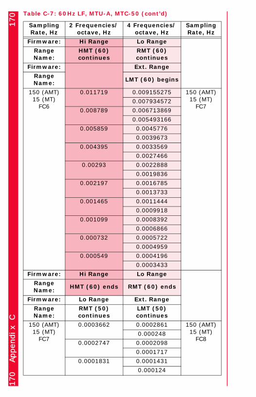
170
Appendix C
170
Firmware: Hi Range Lo Range
Range Name:
HMT (60) continues
RMT (60) continues
Firmware: Ext. Range
Range Name:
LMT (60) begins
150 (AMT)15 (MT)
FC6
0.011719 0.009155275 150 (AMT)15 (MT)
FC70.007934572
0.008789 0.006713869
0.005493166
0.005859 0.0045776
0.0039673
0.004395 0.0033569
0.0027466
0.00293 0.0022888
0.0019836
0.002197 0.0016785
0.0013733
0.001465 0.0011444
0.0009918
0.001099 0.0008392
0.0006866
0.000732 0.0005722
0.0004959
0.000549 0.0004196
0.0003433
Firmware: Hi Range Lo Range
Range Name:
HMT (60) ends RMT (60) ends
Firmware: Lo Range Ext. Range
Range Name:
RMT (50) continues
LMT (50) continues
150 (AMT)15 (MT)
FC7
0.0003662 0.0002861 150 (AMT)15 (MT)
FC80.000248
0.0002747 0.0002098
0.0001717
0.0001831 0.0001431
0.000124
Table C-7: 60Hz LF, MTU-A, MTC-50 (cont’d)
SamplingRate, Hz
2 Frequencies/ octave, Hz
4 Frequencies/ octave, Hz
SamplingRate, Hz

171
Appendix C
171
Shaded areas indicate overlap of frequency ranges.
150 (AMT)15 (MT)
FC7
0.0001373 0.0001049 150 (AMT)15 (MT)
FC80.0000858
0.0000916 0.0000715
0.000062
0.0000687 0.0000525
0.0000429
0.0000458 0.0000358
0.000031
0.0000343 0.0000262
0.0000215
0.0000229 0.0000179
0.0000155
0.0000172 0.0000131
0.0000107
Table C-7: 60Hz LF, MTU-A, MTC-50 (cont’d)
SamplingRate, Hz
2 Frequencies/ octave, Hz
4 Frequencies/ octave, Hz
SamplingRate, Hz

172
Appendix C
172 Table C-8: 60Hz LF, MTU, AMTC-30 (V5-comp.)
SamplingRate, Hz
2 Frequencies/ octave, Hz
4 Frequencies/ octave, Hz
SamplingRate, Hz
Firmware: Up Range Up Range
Range Name:
EMT (60) EMT (60)
3072FC3
768 720 3072FC3624
576 528
432
384 360
312
288 264
216
192 180
156
144 132
108
96 90
78
72 66
54
384FC4
48 45 384FC439
36 33
27
24 22.5
19.5
18 16.5
13.5
12 11.25
9.75
9 8.25
6.75
24FC5
6 5.625 24FC54.875
4.5 4.125
3.375
3 2.8125
2.4375

173
Appendix C
173
24FC5
2.25 2.0625 24FC51.6875
1.5 1.40625
1.21875
1.125 1.03125
0.84375
0.75
0.5625
0.375
0.2813
Table C-8: 60Hz LF, MTU, AMTC-30 (V5-comp.) (cont’d)
SamplingRate, Hz
2 Frequencies/ octave, Hz
4 Frequencies/ octave, Hz
SamplingRate, Hz

174
Appendix C
174 Table C-9: 60Hz LF, MTU, MTC-50 (V5-comp.)
SamplingRate, Hz
2 Frequencies/ octave, Hz
4 Frequencies/ octave, Hz
SamplingRate, Hz
Firmware: D Hi Range
Range Name:
MT (60) MTH (60)
3072FC3
384 360 3072FC3312
288 264
216
192 180
156
144 132
108
96 90
78
72 66
54
384FC4
48 45 384FC439
36 33
27
24 22.5
19.5
18 16.5
13.5
Firmware: D Hi Range
Range Name:
MT (60) continues
MTH (60) continues
Firmware: Ext. Range
Range Name:
LMT (60) begins
384FC4
12 11.25
9.75
9 8.25
6.75
24FC5
6 5.625 24FC54.875
4.5 4.125
3.375
3 2.8125
2.4375

175
Appendix C
175
24FC5
2.25 2.0625 24FC51.6875
1.5 1.40625
1.21875
1.125 1.03125
0.84375
0.75 0.703125
0.609375
0.5625 0.515625
0.421875
Firmware: D, Ext Range Hi Range
Range Name:
MT (60), LMT (60) continue
MTH (60) ends
Firmware: Lo Range
Range Name:
MTL (60)begins
24FC5
0.375 0.3515625
0.3046875
0.2813 0.2578125
0.2109375
0.1875 0.1757813
0.1523438
0.140625 0.1289063
0.1054688
0.09375 0.0878906
0.0761719
0.070646 0.0644531
0.0527344
0.046875 0.0439453
0.0380859
0.035156 0.0322266
0.0263672
24FC6
0.023438 0.0219727 24FC60.019043
0.017578 0.0161133
0.0131836
Table C-9: 60Hz LF, MTU, MTC-50 (V5-comp.) (cont’d)
SamplingRate, Hz
2 Frequencies/ octave, Hz
4 Frequencies/ octave, Hz
SamplingRate, Hz

176
Appendix C
176
Firmware: D, Ext Range Lo Range
Range Name:
MT (60), LMT (60) continue
MTL (60)continues
Firmware: Ext. Range
Range Name:
MTR (60) begins
24FC6
0.011719 0.0109863 24FC60.0095215
0.008789 0.0080566
0.0065918
0.005859 0.0054932
0.0047607
0.004395 0.0040283
0.0032959
0.00293 0.0027466
0.0023804
0.005197 0.0020142
0.0016479
0.001465 0.0013733
0.0011902
0.001099 0.0010071
0.000824
0.000732 0.0006866
0.0005951
0.000549 0.0005035
0.000412
Firmware: D Lo Range
Range Name:
MT (60) ends MTL (60) ends
Firmware: Ext Range Ext. Range
Range Name:
LMT (60) continues
MTR (60)continues
24FC7
0.000366 0.0003433 24FC70.0002975
0.000275 0.0002518
0.000206
0.000183 0.0001717
0.0001488
Table C-9: 60Hz LF, MTU, MTC-50 (V5-comp.) (cont’d)
SamplingRate, Hz
2 Frequencies/ octave, Hz
4 Frequencies/ octave, Hz
SamplingRate, Hz

177
Appendix C
177
Shaded areas indicate overlap of frequency ranges.
24FC7
0.000137 0.0001259 24FC70.000103
0.000092 0.0000858
0.0000744
0.000069 0.0000629
0.0000515
0.000046 0.0000429
0.0000372
0.000034 0.0000315
0.0000257
0.000023 0.0000215
0.0000186
0.000017 0.0000157
0.0000129
Table C-9: 60Hz LF, MTU, MTC-50 (V5-comp.) (cont’d)
SamplingRate, Hz
2 Frequencies/ octave, Hz
4 Frequencies/ octave, Hz
SamplingRate, Hz
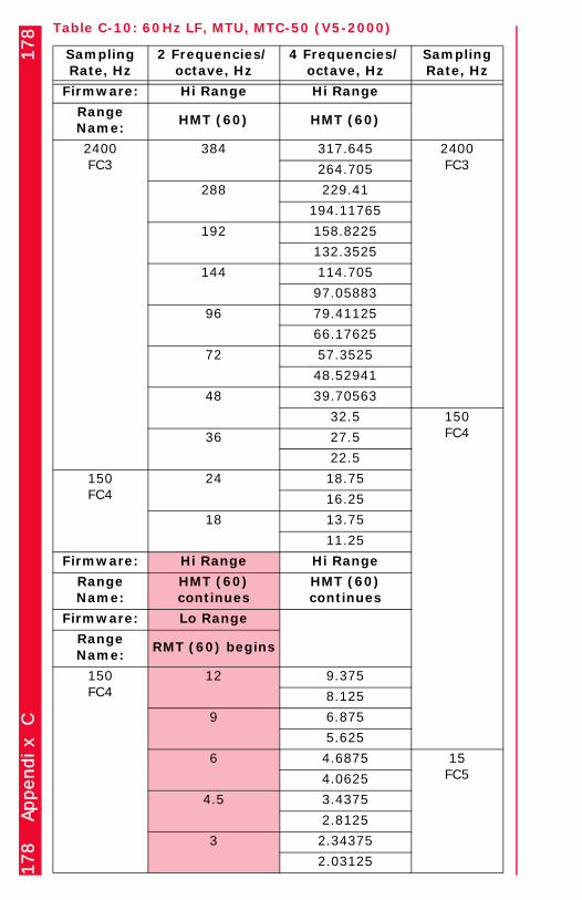
178
Appendix C
178 Table C-10: 60Hz LF, MTU, MTC-50 (V5-2000)
SamplingRate, Hz
2 Frequencies/ octave, Hz
4 Frequencies/ octave, Hz
SamplingRate, Hz
Firmware: Hi Range Hi Range
Range Name:
HMT (60) HMT (60)
2400FC3
384 317.645 2400FC3264.705
288 229.41
194.11765
192 158.8225
132.3525
144 114.705
97.05883
96 79.41125
66.17625
72 57.3525
48.52941
48 39.70563
32.5 150FC436 27.5
22.5
150FC4
24 18.75
16.25
18 13.75
11.25
Firmware: Hi Range Hi Range
Range Name:
HMT (60) continues
HMT (60) continues
Firmware: Lo Range
Range Name:
RMT (60) begins
150FC4
12 9.375
8.125
9 6.875
5.625
6 4.6875 15FC54.0625
4.5 3.4375
2.8125
3 2.34375
2.03125

179
Appendix C
179
150FC4
2.25 1.71875 15FC51.40625
15FC5
1.5 1.171875
1.015625
1.125 0.859375
0.703125
0.75 0.5859375
0.5078125
0.5625 0.4296875
0.3515625
Firmware: Hi, Lo Ranges Hi Range
Range Name:
HMT (60), RMT (60) continue
HMT (60) ends
Firmware: Lo Range
Range Name:
RMT (60) begins
15FC5
0.375 0.2929688 15FC60.2539063
0.28125 0.2148438
0.1757813
0.1875 0.1464844
0.1269532
0.140625 0.1074219
0.0878907
0.09375 0.0732422
0.0634766
0.070313 0.053711
0.0439453
0.046875 0.0366211
0.0317383
0.035156 0.0268555
0.0219727
0.023438 0.0183106
0.0158691
0.017578 0.0134277
0.0109863
Table C-10: 60Hz LF, MTU, MTC-50 (V5-2000) (cont’d)
SamplingRate, Hz
2 Frequencies/ octave, Hz
4 Frequencies/ octave, Hz
SamplingRate, Hz

180
Appendix C
180
Firmware: Hi Range Lo Range
Range Name:
HMT (60) continues
RMT (60) continues
Firmware: Ext. Range
Range Name:
LMT (60) begins
15FC6
0.011719 0.009155275 15FC70.007934572
0.008789 0.006713869
0.005493166
0.005859 0.0045776
0.0039673
0.004395 0.0033569
0.0027466
0.00293 0.0022888
0.0019836
0.002197 0.0016785
0.0013733
0.001465 0.0011444
0.0009918
0.001099 0.0008392
0.0006866
0.000732 0.0005722
0.0004959
0.000549 0.0004196
0.0003433
Firmware: Hi Range Lo Range
Range Name:
HMT (60) ends RMT (60) ends
Firmware: Lo Range Ext. Range
Range Name:
RMT (50) continues
LMT (50) continues
15FC7
0.0003662 0.0002861 15FC80.000248
0.0002747 0.0002098
0.0001717
0.0001831 0.0001431
0.000124
Table C-10: 60Hz LF, MTU, MTC-50 (V5-2000) (cont’d)
SamplingRate, Hz
2 Frequencies/ octave, Hz
4 Frequencies/ octave, Hz
SamplingRate, Hz

181
Appendix C
181
Shaded areas indicate overlap of frequency ranges.
15 FC7
0.0001373 0.0001049 15FC80.0000858
0.0000916 0.0000715
0.000062
0.0000687 0.0000525
0.0000429
0.0000458 0.0000358
0.000031
0.0000343 0.0000262
0.0000215
0.0000229 0.0000179
0.0000155
0.0000172 0.0000131
0.0000107
Table C-10: 60Hz LF, MTU, MTC-50 (V5-2000) (cont’d)
SamplingRate, Hz
2 Frequencies/ octave, Hz
4 Frequencies/ octave, Hz
SamplingRate, Hz

182
Appendix C
182

183 Appendix D 183
Appendix
System 2000 MTU FamilySpecifications
This Appendix provides specifications for the System 2000 family of MTU instruments:• MTU-P (2E, 2H, 3H, 5)• MTU-A (2EA, 2HA, 3HA, 5A)
MTU-P indicates an instrument capable of acquiring MT data, equipped with a pluggable CompactFlash storage card. (Earlier instruments had non-removable storage.)
MTU-A indicates an instrument capable of acquiring MT and AMT data. All versions have removable storage.
The values and specifications given here are typical, and are subject to change. They are not claimed to be worst-case specifications.
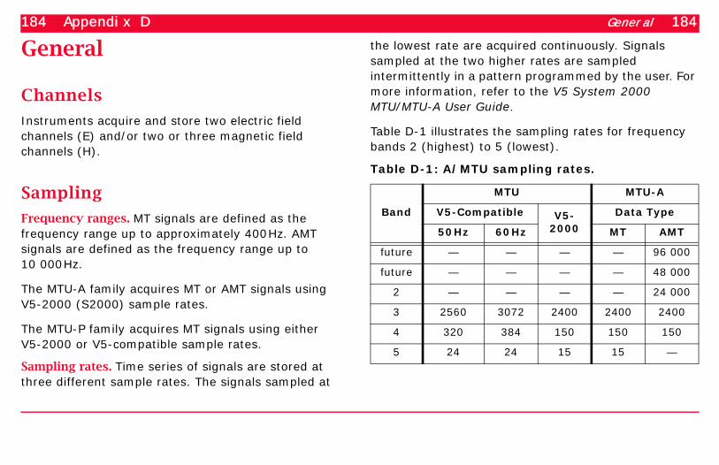
184 Appendix D General 184
General
Channels
Instruments acquire and store two electric field channels (E) and/or two or three magnetic field channels (H).
Sampling
Frequency ranges. MT signals are defined as the frequency range up to approximately 400Hz. AMT signals are defined as the frequency range up to 10 000Hz.
The MTU-A family acquires MT or AMT signals using V5-2000 (S2000) sample rates.
The MTU-P family acquires MT signals using either V5-2000 or V5-compatible sample rates.
Sampling rates. Time series of signals are stored at three different sample rates. The signals sampled at
the lowest rate are acquired continuously. Signals sampled at the two higher rates are sampled intermittently in a pattern programmed by the user. For more information, refer to the V5 System 2000 MTU/MTU-A User Guide.
Table D-1 illustrates the sampling rates for frequency bands 2 (highest) to 5 (lowest).
Table D-1: A/MTU sampling rates.
Band
MTU MTU-A
V5-Compatible V5-2000
Data Type
50Hz 60Hz MT AMT
future — — — — 96 000
future — — — — 48 000
2 — — — — 24 000
3 2560 3072 2400 2400 2400
4 320 384 150 150 150
5 24 24 15 15 —
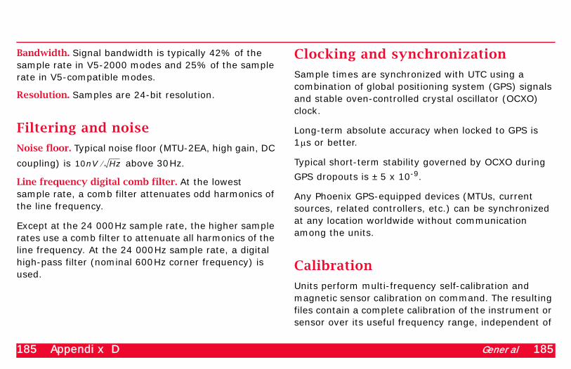
185 Appendix D General 185
Bandwidth. Signal bandwidth is typically 42% of the sample rate in V5-2000 modes and 25% of the sample rate in V5-compatible modes.
Resolution. Samples are 24-bit resolution.
Filtering and noise
Noise floor. Typical noise floor (MTU-2EA, high gain, DC
coupling) is above 30Hz.
Line frequency digital comb filter. At the lowest sample rate, a comb filter attenuates odd harmonics of the line frequency.
Except at the 24 000Hz sample rate, the higher sample rates use a comb filter to attenuate all harmonics of the line frequency. At the 24 000Hz sample rate, a digital high-pass filter (nominal 600Hz corner frequency) is used.
Clocking and synchronization
Sample times are synchronized with UTC using a combination of global positioning system (GPS) signals and stable oven-controlled crystal oscillator (OCXO) clock.
Long-term absolute accuracy when locked to GPS is 1µs or better.
Typical short-term stability governed by OCXO during
GPS dropouts is ±5 x 10⁻⁹.
Any Phoenix GPS-equipped devices (MTUs, current sources, related controllers, etc.) can be synchronized at any location worldwide without communication among the units.
Calibration
Units perform multi-frequency self-calibration and magnetic sensor calibration on command. The resulting files contain a complete calibration of the instrument or sensor over its useful frequency range, independent of
10nV Hz⁄
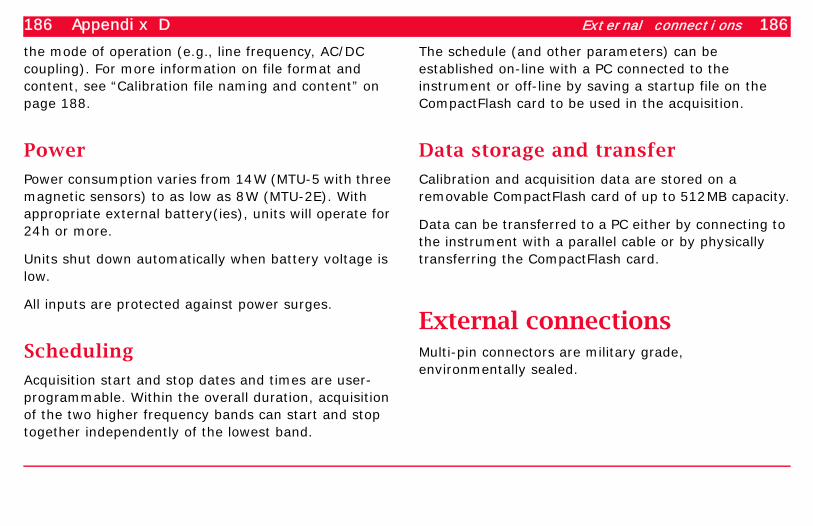
186 Appendix D External connections 186
the mode of operation (e.g., line frequency, AC/DC coupling). For more information on file format and content, see “Calibration file naming and content” on page 188.
Power
Power consumption varies from 14W (MTU-5 with three magnetic sensors) to as low as 8W (MTU-2E). With appropriate external battery(ies), units will operate for 24h or more.
Units shut down automatically when battery voltage is low.
All inputs are protected against power surges.
Scheduling
Acquisition start and stop dates and times are user-programmable. Within the overall duration, acquisition of the two higher frequency bands can start and stop together independently of the lowest band.
The schedule (and other parameters) can be established on-line with a PC connected to the instrument or off-line by saving a startup file on the CompactFlash card to be used in the acquisition.
Data storage and transfer
Calibration and acquisition data are stored on a removable CompactFlash card of up to 512MB capacity.
Data can be transferred to a PC either by connecting to the instrument with a parallel cable or by physically transferring the CompactFlash card.
External connectionsMulti-pin connectors are military grade, environmentally sealed.

187 Appendix D Mechanical and environmental 187
Ground
An external binding post provides the case ground, which should be connected to a porous pot electrode.
Telluric inputs
Units are equipped with four binding posts, marked WNSE for ease of cable connection.
Parallel port
A multi-pin connector is used for control and data transfer via an external adapter.• Circular, 26-pin, shell size 16.• Pinouts compatible with IEEE 1284 ECP bidirectional
PC parallel port (pin A = PC pin 1, pin B = PC pin 2, etc.).
• Electrostatic discharge protection on all pins.• 5V logic levels.
Auxiliary connector• Circular, 18-pin, shell size 14.• Provides signal input, power output, and calibration
signals to three magnetic sensors.
Battery connector• Circular, 4-pin, shell size 8.• Surge protection and overload protection on all pins.• Pin A: Battery 1, +12VDC.• Pin B: Battery 2, +12VDC.• Pin C: Battery common.• Pin D: Battery common.
GPS antenna connector• Circular, BNC-type.
Mechanical and environmentalCase. Environmentally sealed diecast aluminum.

188 Appendix D File types and logical record formats 188
Weight. 4.4kg.
Dimensions. 230mm x 225mm x 110mm.
Operating temperature. –20°C to +50°C.
File types and logical record formatsResults are stored in the files described in the following paragraphs. To allow future changes in file formats to be made transparent, Phoenix software uses a library of C-language functions to access the files. Anyone writing software to access files generated by the MTU family is strongly advised to used the Phoenix C library.
Calibration file naming and content
Calibration files are in a proprietary binary format. Human-readable calibration information can be extracted from calibration files by supplying the SYSCAL program with a text file of frequencies.
SYSCAL then computes and displays the response of the instrument or sensor at those frequencies.
Instrument. Instrument calibration files are named automatically in the format ssss.CLB, where ssss is the instrument serial number.
Sensors. Sensor calibration files are named by the user, and should be in the format COILssss.CLC (for MTC-50 sensors), AMTCssss.CLC (for MTC-30 sensors), or LOOPssss.CLC (for AL-100 airloop sensors), where ssss is the coil or loop serial number.
Time series file naming and content
Time series files can be named by the user. If the user does not supply a name, files are named automatically in the format ssssmdda, where
• ssss is the instrument serial number• m is the month in hexadecimal• dd is the day in decimal• a is an alpha character denoting the order of
repeated soundings on the same day.

189 Appendix D File types and logical record formats 189
The file extension is in the format TSH, TSL, or TSn and denotes the sample rate:
.TSH = V5-compatible Bands 3 and 4 sample rates.
.TSL = V5-compatible Band 5 sample rates.
.TS2 = 24 000Hz sample rate.
.TS3 = 2400Hz sample rate.
.TS4 = 150Hz sample rate.
.TS5 = 15Hz sample rate.
Note TS2 to TS5 may use other sample rates in the future. TSH and TSL apply only to MTU instruments in V5-compatible modes.
Time series file format
Time series files consist of records containing time series data, written chronologically from the time of the first sample in the record.
Record lengths within a single file may vary.
Each record consists of a tag followed by time series data. Figure D-1 on page 190 illustrates the file format graphically.
The time series is stored in 24-bit two’s complement format, three bytes per sample, least significant byte first. A scan is a set of samples, one from each channel, taken simultaneously. A complete scan from one sample time is stored consecutively in order of channel number. (Channels are numbered starting at 1, not 0.) Scans are stored in order of sample time.
The first scan in a record always starts exactly on a UTC second, and the scan rate is always an exact integer multiple of 1Hz.

190 Appendix D File types and logical record formats 190
Figure D-1: A graphical representation of the time series file format. The scans within one record span either one second (Bands 3, 4, and 5) or 0.1 second (Band 2). Records always begin on a UTC second, but not necessarily on consecutive UTC seconds.
Time series tag format
The tag format may vary depending on instrument firmware, but only one tag format is used in any one file.
Currently, tags are 16 bytes long in TSH and TSL files and 32 bytes long in TSn files. Table D-1 summarizes the byte assignments within the tags, and the paragraphs that follow provide additional detail.
(16 or 32 bytes)
Ch1 Ch2 Chn...
Scan0
Ch1 Ch2 Chn...
Scan1 ...
Ch1 Ch2 Chn...
ScannTag0
Ch1 Ch2 Chn...
Scan0
...etc.
Record0 Record1
Ch1 Ch2 Chn...
Scan1 ...
Ch1 Ch2 Chn...
Scann... Tag1
(16 or 32 bytes)
Simultaneoussamples
UTCsecond
UTCsecond
= 1 byteCh = Channel

191 Appendix D File types and logical record formats 191
Bytes 10–11. The number of scans in the record. Except in TS2 files, every record contains 1s of data, so this 16-bit integer is also the sample rate in Hz. (TS2 records contain 0.1s of data.)
Byte 13. In TSn files, this byte contains the tag length in bytes (currently 32). In TSL and TSH files, this byte contains the code 0, indicating a 16-byte tag length.
Byte 14. The instrument status code values are explained in Table D-3.
Table D-2: Summary of tag byte assignments
Byte Meaning
0–7 UTC time of first scan in the record.
0 second
1 minute
2 hour
3 day
4 month
5 year (last 2 digits)
6 day of week
7 century
8–9 instrument serial number (16-bit integer)
10–11 number of scans in the record (16-bit integer)
12 number of channels per scan
13 tag length (TSn) or tag length code (TSH, TSL)
14 status code
15 bit-wise saturation flags
Tags in TSH or TSL files end with byte 15
16 reserved for future indication of different tag and/or sample formats
17 sample length in bytes
18–19 sample rate (in units defined by byte 20)
20 units of sample rate
21 clock status
22–25 clock error in µs
26–31 reserved; must be 0
Table D-2: Summary of tag byte assignments
Byte Meaning

192 Appendix D File types and logical record formats 192
Byte 15. Saturation flags. Each bit corresponds to a different channel (bit 0 for channel 1, bit 1 for channel 2, etc.). A bit’s value will be 1 if either the common mode or differential mode input voltage limit is exceeded in any sample.
Byte 16. This byte is reserved for future use to identify different tag formats or different sample formats, such
as floating point or compressed format. The value is currently 0.
Byte 17. The sample length in bytes, currently 3. Future changes in sample formats (32-bit integer or floating point, for example) may cause this value to change.
Bytes 18–19. The sample rate (per unit time as specified by Byte 20). For the range of possible values, see Table D-1 on page 184.
Byte 20. Time unit of the sample rate. The current range of values is shown in Table D-4. Other values may be defined in the future.
Byte 21. Clock status. This byte reflects the status of the clock at the time the record is taken. A value of 4
Table D-3: Status codes (Tag Byte 14)
Value Meaning
0 normal completion
1 internal error
2 reserved
3 saturation of front-end board analog circuits
4 internal error in front-end board digital signal pro-cessor (DSP)
5 internal error
6 processor timed out without receiving data from front-end board DSP
7 internal error
8 internal error
Table D-4: Sample rate units (Tag Byte 20)
Value Unit
0 second (Hz)
1 minute
2 hour
3 day

193 Appendix D Related products 193
indicates that the clock was locked to GPS. A value of 3 indicates that the time is based on the crystal oscillator initialized by GPS.
Bytes 22–25. Clock error in µs. The value will be 0 unless GPS lock has been lost and reacquired. Recovery from GPS dropout (re-synchronization of the crystal oscillator) can take up to 20min. During this time, the difference between the recorded sample time (bytes 0–7) and the actual sample time is recorded as clock error. This value is a 32-bit two’s complement integer, positive if the sample is late, negative if it is early.
Related productsSeveral other products for similar or specialized applications are available or under development.
MTU-TXC
Used to synchronize other equipment, such as current sources, to System 2000 equipment.
UTC signal output:
• 921 600Hz• 1Hz• 1/60Hz
Geophysical current source control output:
• 0.001Hz to 10kHz
Control waveforms are referenced to zero phase at UTC 2000 Jan 01 00:00:00.
MTU-2ESD, MTU-5ESD
Used in remote reference and monitoring applications, these instruments use a 33.6kb/s dialup telephone connection for control and data transfer.
MTU-2ES, MTU-5S
Also used in monitoring applications, these instruments use a serial interface for control and data transfer, typically connecting to a fibre optic or copper wire modem.

194 Appendix D Related products 194
MTU-5LR
Used in surveys with extended depths of investigation, these instruments employ a ring-core fluxgate magnetic sensor and low sample rates.
MTU-AI family
These instruments, under development in 2003, provide an infrared interface to allow setup and monitoring from Palm OS® handheld terminals.
System2000.net family
These instruments, introduced in 2004, are multichannel, multifunction receivers. The family includes the V8 and RXU receivers and the RXU-TM transmitter controller. The V8 has a full-colour, sunlight-readable display and keyboard, while the RXUs are equipped with an infrared interface and are sold with Palm OS® handheld terminals. All the instruments can optionally be equipped with wireless network capability.

195 Index 195
Index
Numerics2 frequencies per octave, 414 frequencies per octave, 414096, error code, 1344097, error code, 1344098, error code, 13454, ECP driver error code, 134
Aabout the software, 2AC coupling, examining calibrations, 44acquisition times, verifying,
SSMT2000, 23Adaptive Scale, SyncTSV, 114Adaptive scale, SyncTSV, 113advanced crosspower parameters, 39Advanced Parameter Table Interface, 48Analyse TS files, SyncTSV, 113archiving raw data, SSMT2000, 15array type, changing, 64ATYP, 64audience, intended, 2
AutoEdit, 82AutoX, 94
Bbands, processing, 41bandwidth, specifications, 181batch processing, SSMT2000, 34
Ccalibration
curves, printing, 45files, examining, 42viewing data numerically, 46
channels, specifications, 180ChartEditor, 93Circle tool, MT-Editor, 83CLB file extension, 42CLC file extension, 42clocking and synchronization,
specifications, 181CMOS Setup, ECP port, 131coherencies, viewing in SyncTSV, 120coherency, 36
coherency type, 37coherent noise, 38comb filter, 181communications, parallel port
troubleshooting, 133compatibility mode, Windows XP, 134Component Pairs legend, SyncTSV, 120connection errors, magnetic, 52connections
specifications, 182controls, resizing in MT-Editor, 92Copy Files command, SSMT2000, 11correcting layout errors, 49corrupt file, editing, SSMT2000, 47Create Fourier Coefficients (TS to FT)
command, noise tests, SSMT2000, 65
Create Fourier Coefficients (TS to FT) command, SSMT2000, 27
creating Fourier transforms, SSMT2000, 24
crosspower parameters, 38custom parameters report, 60customizing graphs, MT-Editor, 94

196 Index 196
Ddata processing flowchart, 125data processing overview, 6data storage and transfer,
specifications, 182DC offset, SyncTSV, 113default times, Fourier Transform
parameter, 42DEFAULT.PFT, examining calibrations, 44DEFAULT.TBL, examining calibrations, 44degrees, report format, 61Deleting tool, MT-Editor, 84Device Manager, Windows, 130, 132digital comb filter, 181diting, 35DMF, latitude and longitude format, 61DMS, latitude and longitude format, 61DXAC, 22DXDC, 22DYAC, 22DYDC, 22
EECP driver, use of interrupt, 134ECP printer port, 130EDI format, exporting from MT-
Editor, 103EDI, latitude and longitude format, 61Edit Robust Parameters (PRM) command,
SSMT2000, 28, 35Edit TS to FT Parameters (PFT)
command, SSMT2000, 25, 65editing crosspowers, MT-Editor, 97Editing tool, MT-Editor, 82electrode resistance and calibration, 43E-line electrical values, 22E-line errors, correcting, 53EMT file extension, 76error codes, parallel port
4096, 1344097, 1344098, 13454, 134
error messagesSyncTSV, 116
evaluating noise test plots, 73EXAC, 22examining calibration files, 42Excel, for reports, 62EXDC, 22export options, MT-Editor, 84exporting in EDI format, MT-Editor, 103exporting, MT-Editor, 135extended bands, 41Extended Capability Port (ECP), 130extensions, file, 9external connections, specifications, 182EYAC, 22EYDC, 22
FFAQs, 3FCn file extension, 27FCn file extension, noise tests, 66file and folder names, Plot Files, 30file extension, Plot Files, 28file extensions, SSMT2000, 9file names, raw data, SSMT2000, 10file naming, specifications, 184files, organizing, 136filtering and noise, specifications, 181flowchart, data processing, 125folder and file names, 9format
data records, 184format, latitude and longitude in
reports, 61Fourier Transform parameters, 39Freq. Scale legend, SyncTSV, 118frequencies, specifying in MT-Editor, 86frequency
ranges, specifications, 180frequency ranges
specifications, 180frequency ranges, instrument/sensor
combinations, 41frequency tables,SSMT2000, 141FT, samples for, SyncTSV, 116
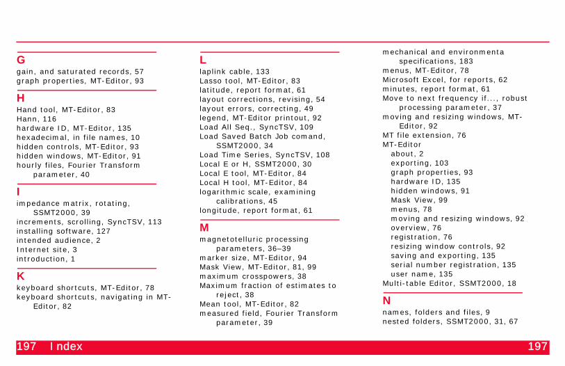
197 Index 197
Ggain, and saturated records, 57graph properties, MT-Editor, 93
HHand tool, MT-Editor, 83Hann, 116hardware ID, MT-Editor, 135hexadecimal, in file names, 10hidden controls, MT-Editor, 93hidden windows, MT-Editor, 91hourly files, Fourier Transform
parameter, 40
Iimpedance matrix, rotating,
SSMT2000, 39increments, scrolling, SyncTSV, 113installing software, 127intended audience, 2Internet site, 3introduction, 1
Kkeyboard shortcuts, MT-Editor, 78keyboard shortcuts, navigating in MT-
Editor, 82
Llaplink cable, 133Lasso tool, MT-Editor, 83latitude, report format, 61layout corrections, revising, 54layout errors, correcting, 49legend, MT-Editor printout, 92Load All Seq., SyncTSV, 109Load Saved Batch Job comand,
SSMT2000, 34Load Time Series, SyncTSV, 108Local E or H, SSMT2000, 30Local E tool, MT-Editor, 84Local H tool, MT-Editor, 84logarithmic scale, examining
calibrations, 45longitude, report format, 61
Mmagnetotelluric processing
parameters, 36–39marker size, MT-Editor, 94Mask View, MT-Editor, 81, 99maximum crosspowers, 38Maximum fraction of estimates to
reject, 38Mean tool, MT-Editor, 82measured field, Fourier Transform
parameter, 39
mechanical and environmenta specifications, 183
menus, MT-Editor, 78Microsoft Excel, for reports, 62minutes, report format, 61Move to next frequency if..., robust
processing parameter, 37moving and resizing windows, MT-
Editor, 92MT file extension, 76MT-Editor
about, 2exporting, 103graph properties, 93hardware ID, 135hidden windows, 91Mask View, 99menus, 78moving and resizing windows, 92overview, 76registration, 76resizing window controls, 92saving and exporting, 135serial number registration, 135user name, 135
Multi-table Editor, SSMT2000, 18
Nnames, folders and files, 9nested folders, SSMT2000, 31, 67

198 Index 198
No acceptable time segments found, SyncTSV, 116
noise test results, viewing, 70noise, coherent, 38North Reference, SSMT2000, 22NPIPlot, 69NPIPlot, appearance, 72NPIPlot, printing, 72Nuttall, 116
Oon-line support, 3Oplog Lines, MT-Editor, 81Options menu, SyncTSV, 111Options tool, MT-Editor, 82organizing your files, 136
Pparallel noise data, processing, 64Parallel Noise Processing (PRM)
command, SSMT2000, 67parallel noise test, Fourier Transform
parameter, 40parallel noise tests, evaluating, 73parallel port
configuring, 130troubleshooting communications, 133
PC requirements, 128PFT file extension, 24PFT File Naming Convention, table, 24
Phoenix Geophysics Limited, contact information, 3
plot appearance, NPIPlot, 72Plot Files, 28PLOT-COMP, 88, 89PLOT-EDIT, 88, 89Pointer tool, MT-Editor, 83Polar Diagrams, 81polar diagrams, viewing, MT-Editor, 101polarity errors, magnetic, 51Ports (COM & LPT), 132power spectra density, SyncTSV, 120power spectra, SyncTSV, 115power spectra, viewing in SyncTSV, 115power, specifications, 182printer setup, SyncTSV, 123printing calibration curves,
SSMT2000, 45printing noise test plots, 72printing, MT-Editor, 102printing, SyncTSV, 121PRM file extension, 28processing flowchart, 125processing times, SSMT2000, 42PSD, 120
Rraw data file names, SSMT2000, 10record formats, 184Rectangular (power spectra),
SyncTSV, 116reference channels, SSMT2000, 30registering MT-Editor, 135related products, specifications, 189Remote E or H, SSMT2000, 30Remote E tool, MT-Editor, 84remote H reference channels, MT-
Editor, 89Remote H tool, MT-Editor, 84Remove linear phase delay, examining
calibrations, 44renaming data files, SSMT2000, 15reports
creating, 57custom parameters, 60importing to spreadsheet, 62latitude and longitude formats, 61modifying custom parameters
reports, 61saturated records, 57time ranges, 23, 57view site parameters, 18, 57
Reprocess (Robust) command, SSMT2000, 33, 68
requirements, PC, 128resistivity variance, 37resizing or restoring window controls,
MT-Editor, 92resolution, specifications, 181Restore Defaults, SyncTSV, 115
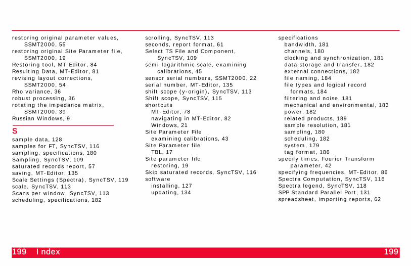
199 Index 199
restoring original parameter values, SSMT2000, 55
restoring original Site Parameter file, SSMT2000, 19
Restoring tool, MT-Editor, 84Resulting Data, MT-Editor, 81revising layout corrections,
SSMT2000, 54Rho variance, 36robust processing, 36rotating the impedance matrix,
SSMT2000, 39Russian Windows, 9
Ssample data, 128samples for FT, SyncTSV, 116sampling, specifications, 180Sampling, SyncTSV, 109saturated records report, 57saving, MT-Editor, 135Scale Settings (Spectra), SyncTSV, 119scale, SyncTSV, 113Scans per window, SyncTSV, 113scheduling, specifications, 182
scrolling, SyncTSV, 113seconds, report format, 61Select TS File and Component,
SyncTSV, 109semi-logarithmic scale, examining
calibrations, 45sensor serial numbers, SSMT2000, 22serial number, MT-Editor, 135shift scope (y-origin), SyncTSV, 113Shift scope, SyncTSV, 115shortcuts
MT-Editor, 78navigating in MT-Editor, 82Windows, 21
Site Parameter Fileexamining calibrations, 43
Site Parameter fileTBL, 17
Site parameter filerestoring, 19
Skip saturated records, SyncTSV, 116software
installing, 127updating, 134
specificationsbandwidth, 181channels, 180clocking and synchronization, 181data storage and transfer, 182external connections, 182file naming, 184file types and logical record
formats, 184filtering and noise, 181mechanical and environmental, 183power, 182related products, 189sample resolution, 181sampling, 180scheduling, 182system, 179tag format, 186
specify times, Fourier Transform parameter, 42
specifying frequencies, MT-Editor, 86Spectra Computation, SyncTSV, 116Spectra legend, SyncTSV, 118SPP Standard Parallel Port, 131spreadsheet, importing reports, 62
200 Index 200
SSMT2000about, 2batch processing, 34Create Fourier Coefficients (TS to FT)
command, 27Create Fourier Coefficients (TS to FT)
command, noise tests, 65creating data folders, 9Edit Robust Parameters (PRM)
command, 28, 35Edit Site Parameters command, 21Edit TS to FT Parameters (PFT)
command, 25, 65Fourier transforms, creating, 24frequency tables, 141Load Saved Batch Job command, 34main window, 8Multi-table Editor, 18North Reference, 22Parallel Noise Processing (PRM)
command, 67processing times, 42renaming data files, 15Reprocess (Robust) command, 33, 68selecting folders and files, 9sensor serial numbers, 22starting, 8temporary file size, 31Toggle Fields command, 21transferring data to your PC, 9
verifying acquisition times, 23verifying site parameters, 17View Ranges command, 31View Site Parameters command, 18, 57View Time Ranges, 23, 57
start and end times, specifying, SyncTSV, 111
Starting Data, MT-Editor, 81starting MT-Editor, 78starting SSMT2000, 8station header, MT-Editor, 81Status bar, SyncTSV, 110Std View, MT-Editor, 82support, contact information, 3support, on-line, 3Synchro Time Series View
about, 3SyncTSV, 105
shift scope, 113troubleshooting time series files, 112
System 2000, 2System 2000.net, 2
Ttag format, specifications, 186TBL (site parameter) file, 17TBO file extension, 18telluric component errors, correcting, 53temporary file size, SSMT2000, 31time span of acquisition, 23
Tipper magnitude scale, MT-Editor, 94Toggle Fields command, SSMT2000, 21toolbars, MT-Editor, 80troubleshooting time series files,
SyncTSV, 112Two Vertical Lines tool, MT-Editor, 83
Uupdating software, 134URL, Phoenix Web site, 3user name, MT-Editor, 135
Vverifying acquisition times,
SSMT2000, 23verifying site parameters, SSMT2000, 17vertical scale, examining calibrations, 45Vertical Scales, SyncTSV, 114View Ranges command, SSMT2000, 31View Site Parameters command,
SSMT2000, 18, 57View Time Ranges command,
SSMT2000, 23, 57viewing noise test results, 70
WWeb site, 3weight cutoff value, 38weight type (Rho variance, Ordinary
coherency), 38
201 Index 201
white noise test, Fourier Transform parameter, 39
Windows Me, installation procedure, 129Windows shortcuts, SSMT2000 Multi-
table Editor, 21Windows XP and ECP port, 133Windows XP, compatibility mode, 134Windows, Russian, 9
ZZoom (spectra), SyncTSV, 119