Data preparation, data presentation, and basic principles of statistics

Gary CollinsEQUATOR Network, Centre for Statistics in Medicine

NDORMS, University of Oxford

EQUATOR Network – OUCAGS training course25 October 2014

2

Summary of last session

“To consult the statistician after an experiment

is finished is often merely to ask him to conduct a post mortem examination. He can perhaps say what the experiment died of.”

R.A. Fisher (1938)

Statistics plays a huge part in research, not just at the analysis stage

• Have a good research question and an appropriate study designcan answer this question

• Protocols are invaluable and should be written for all research studies

3

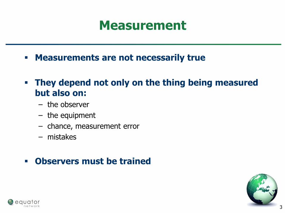
Measurement

Measurements are not necessarily true

They depend not only on the thing being measured but also on:

– the observer

– the equipment

– chance, measurement error

– mistakes

Observers must be trained

4

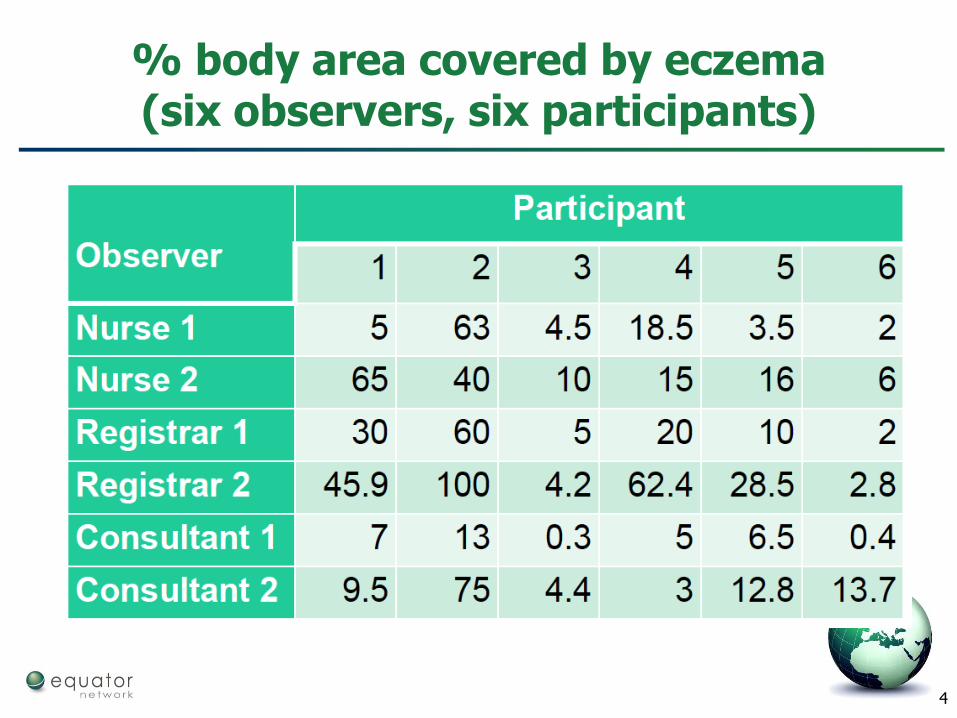
% body area covered by eczema(six observers, six participants)

5

Outline of today

1. Data preparation

1. Basic principles of statistics– introducing some key concepts of statistical inference

----------------------------Break----------------------------

2. Principles of sample size calculations / further data analysis topics

3. Issues to consider in critical appraisal

6

Outline of this session

To understand the importance of data preparation– prospective data collection

To understand why knowing your data is important

To understand the key principles of statistics– inference, uncertainty and bias, confidence intervals,

hypothesis testing

To understand issues in critically appraising a published research article

7

Data preparation

Prior to ANY data analysis it is important to check the data

– often more time is spent ‘cleaning’ and examining the data than the actual analysis

– reliable results rely on accurate and reliable data

• garbage in garbage out

Data accuracy can be improved by prospectively thinking about the data before collecting it

– produce a data collection sheet

– set up database

– is possible, include basic checks in the database

• often done for clinical trials

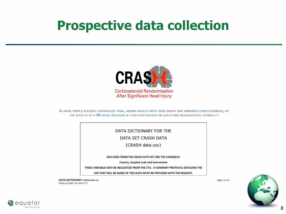
8

Prospective data collection

9

Data Definitions (CRASH dataset)

Variable Label Comments Max length

Type Codes

Patient ID Six digit unique identifier

treatmentbox-pack number

7 string

Sex Gender of the patient

1 Number 0=Male1=Female

DOB Date of birth of the patient

DD/MM/YYYY 10 Date -7303=DOB not known

TRAND Time of randomisation

HH:MM:SSS 8 Time

GCS_EYE Glasgow ComaScale: Eye opening

1 Number 4=spontaneous3=to sound2=to pain1=none

10

Data preparation (after collection)

For data types

– discrete (e.g. number of children): check for non-integer values

– continuous (e.g. height): check values line in plausible range

– binary (e.g. male/female)

– nominal (e.g. blood type)

– ordinal (e.g. cancer stage)

– dates: check for valid dates, date of event before date of birth

– most statistical software doesn’t by default differentiate between upper and lower case (e.g. yes, Yes, yES, yeS, yES, Yes, YeS, YES)

Missing data: consistency in how this is recorded

– how much is missing

Check for unlikely values

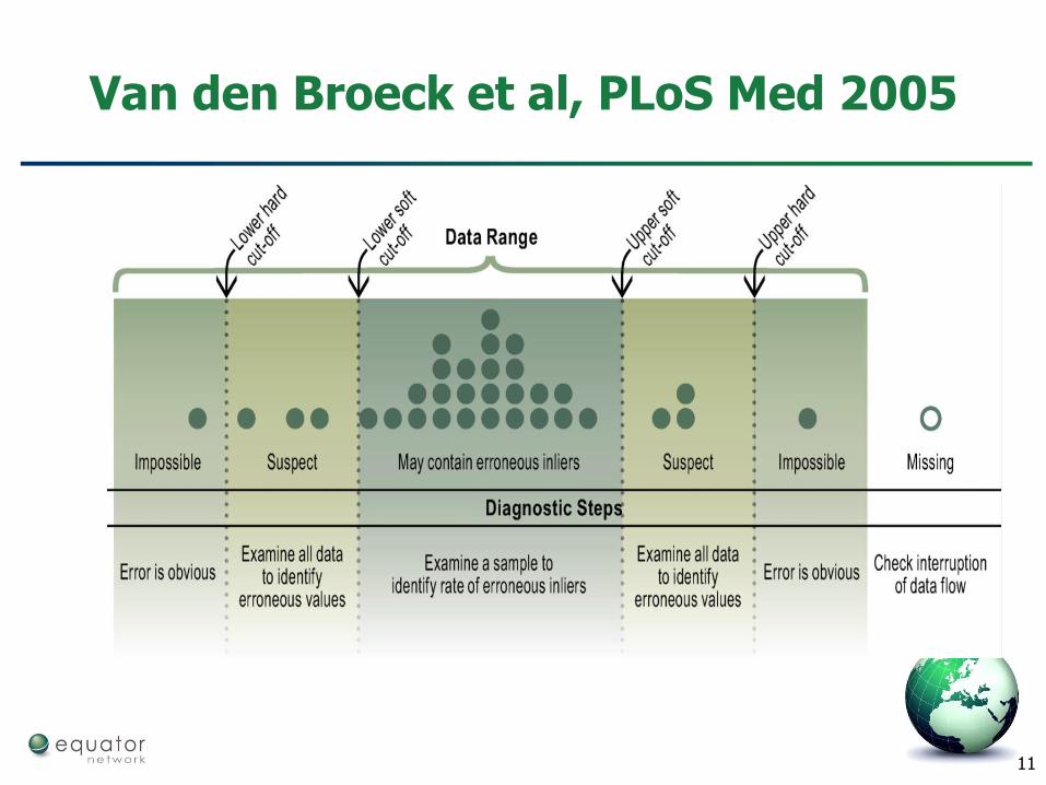
11

Van den Broeck et al, PLoS Med 2005

12

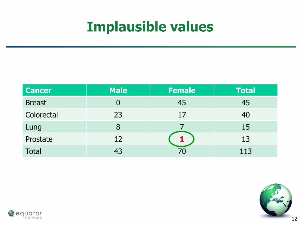
Implausible values

Cancer Male Female Total

Breast 0 45 45

Colorectal 23 17 40

Lung 8 7 15

Prostate 12 1 13

Total 43 70 113

13

Outliers

• Outliers will seem incompatible with the rest of the data

• May deviate from the main body of the data

• Usually extreme values (high or low)

• Can be genuine observations

• Have considerable influence on the results

• Any suspicious values should be checked

• The decision to include or exclude outliers should be made with caution

Provided all the measurements are valid, often useful to analyse with and without the outlier

14

Data presentation (exploration/presentation)

Plot the data, plot the data, plot the data !!!

– prior to any statistical analysis – look at the data!

– get familiar with the data – what does it look like

– can highlight/indicate any errors (spurious values) in the data part of data cleaning)

– what is the distribution of the data (univariate)?

• do they have an approximate Normal distribution?

• if not, can they be transformed (e.g. log transformation)?

Plot the data, plot the data, plot the data !!!

15

Unfortunately, not all data look like this

16

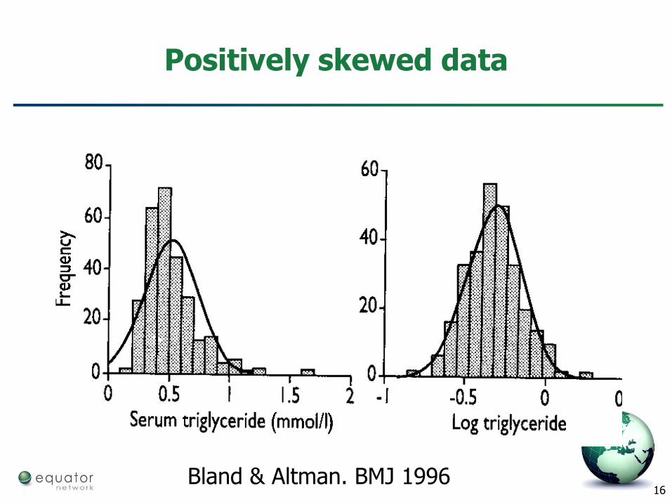
Positively skewed data

Bland & Altman. BMJ 1996

17

CRASH-2 trial(distribution of baseline Glasgow Coma Score)

18

19

20

Data presentation (exploration/presentation)

Where possible, plot the raw values

– there is NO reason to hide it

– let the data tell the story

Beware of ‘chartjunk’ (Edward Tufte)

– anything that distracts the viewer (including you) from the information that graph is intended to present

– let the data speak for themselves, don’t clutter the plot

21

Dynamite plots

Schriger & Cooper. Ann Emerg Med 2001

Mean=82 mmMean=77 mm

22

Dynamite plots

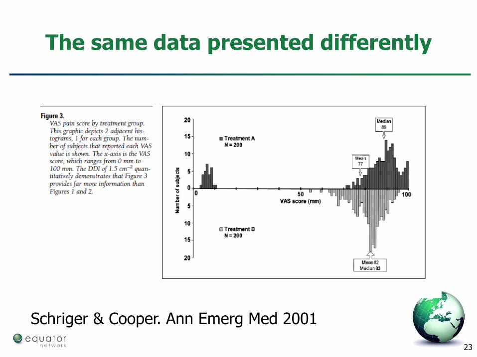
23

The same data presented differently

Schriger & Cooper. Ann Emerg Med 2001

24

Boxplots

25

Sample (Placebo)Sample (Active treatment)

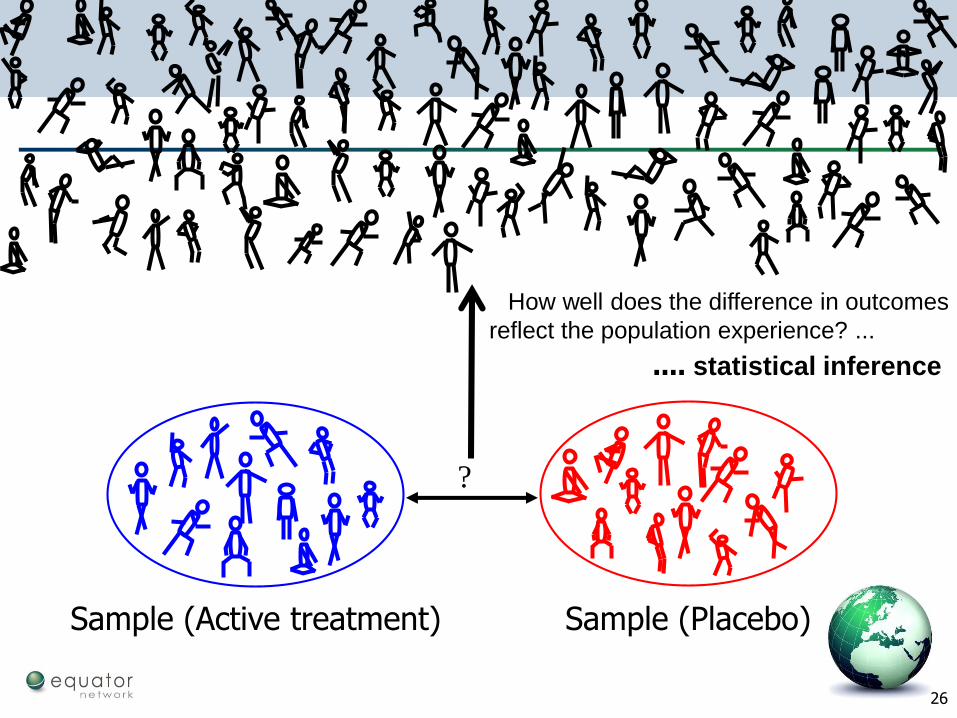
Populations and samples

26

Sample (Placebo)Sample (Active treatment)

?

How well does the difference in outcomes

reflect the population experience? ...

.... statistical inference

27

Basic statistical principles

Information observed from a sample (e.g. single clinical trial) is used to make inferences about a population

Uncertainty (sampling variation)

– the sample value (e.g. treatment effect) is used as the ‘best estimate’ of the population value

– but how good an estimate is it?

– small studies have much uncertainty

A carefully chosen sample can yield reliable answers whereas an unrepresentative (biased) sample produces misleading conclusions

– e.g. in recruitment, follow-up, measurement etc…

28

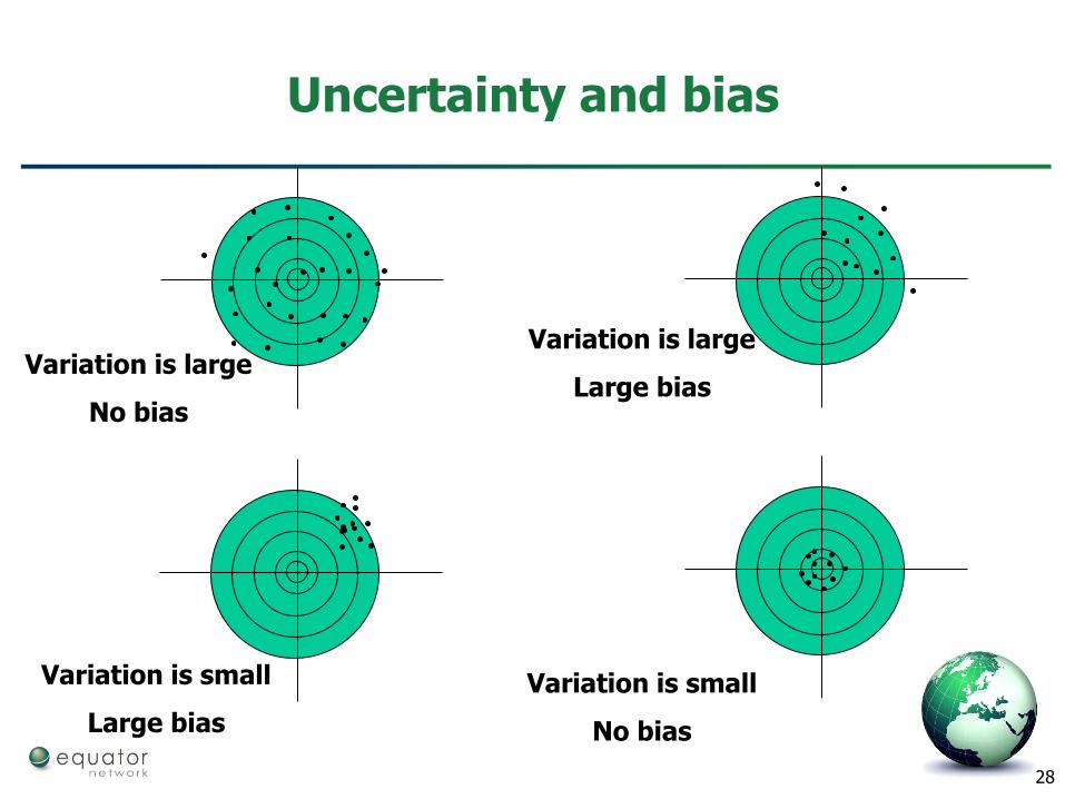
Uncertainty and bias

Variation is large

No bias

Variation is large

Large bias

Variation is small

Large bias

Variation is small

No bias

29

Uncertainty and bias

A single (point) estimate (sample value) is of limited usefulness as it doesn’t reveal the uncertainty associated with the estimate

We can quantify uncertainty

– standard error

– confidence interval

30

Measuring variability

Standard deviation (SD)

– Variability of one sample

Small SD => the data are close to the mean

Large SD => the data are far from the mean

SD = square root of the variance

31

Measuring uncertainty

We are usually interested in the mean (or some other estimate, e.g. proportion) of the population

– so how good is the sample estimate?

Repeat the study lots of times

– sample means will vary (sampling distribution)

– we can calculate the mean and standard deviation (SD) of the sampling distribution (standard error of the mean, SE)

32

Results from a single study (n=100)True mean=35; SD=6

SD=5.6

33

Results from 5 studies (n=100) (same population)

SD=5.6, 5.2, 6.0, 5.5, 5.6

34

Results from 10 studies (n=100) (same population)

SD=5.6, 5.2, 6.0,…6.0, 5.7, 6.5

35

Results from 100 studies (n=100) (same population)

36

Measuring uncertainty

We are usually interested in the mean (or some other estimate, e.g. proportion) of the population

– So how good is the sample estimate?

Repeat the study lots of times

– Sample means will vary (sampling distribution)

– We can calculate the mean and standard deviation of the sampling distribution (standard error of the mean, SE)

– Impractical => not needed

However, a fundamental result in statistics is that the SE = SD/√(sample size)

– Depends only on the sample standard deviation and it’s sample size

37

Sampling distribution

True mean=35, SD=6

Means of 1000 samples of size 100

mean=34.99; SD=0.6;

38

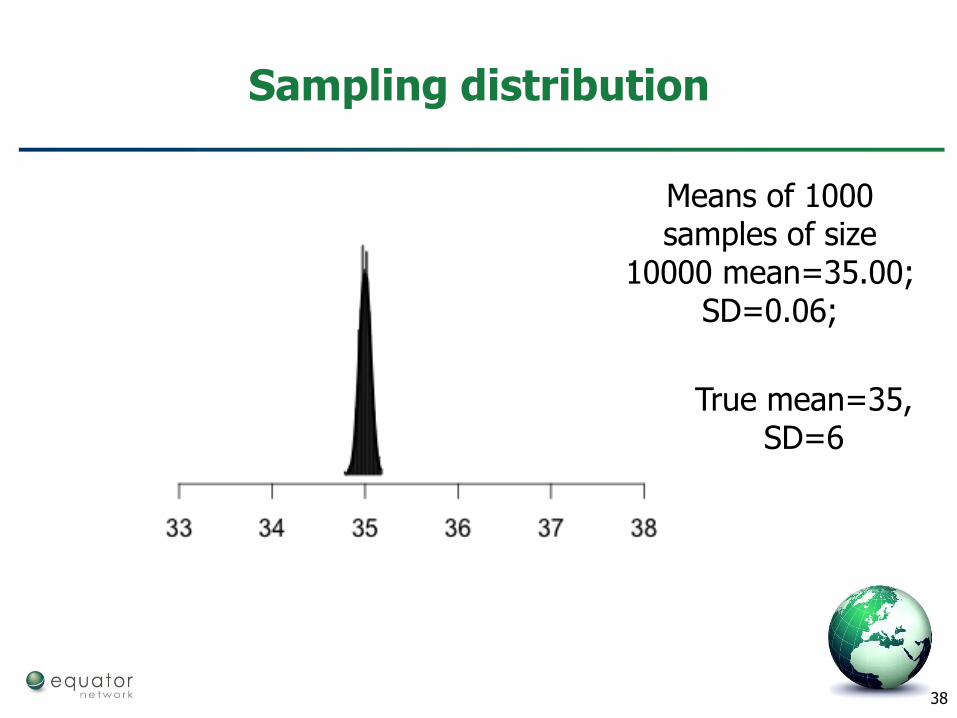
Sampling distribution

Means of 1000 samples of size

10000 mean=35.00; SD=0.06;

True mean=35, SD=6

39

Standard error

Quantifies how far the sample value might be from the true (but unknown) population value

– Assumes that the sample is representative (unbiased)

– Indicates variability due just to sampling variation

SE decreases as the sample size increases

Its main value is as the basis for calculation of a confidence interval

40

Confidence Interval (CI)

Range of values which we can be confident includes the true value

Usually 95% CI

– The 95%CI is the range of values which we are confident (usually 95%) includes the true (population) value

95% CI is approximately

Estimate ± 2 SE

As sample size increases

– uncertainty decreases

– Standard error gets smaller

– width of confidence interval reduces

41

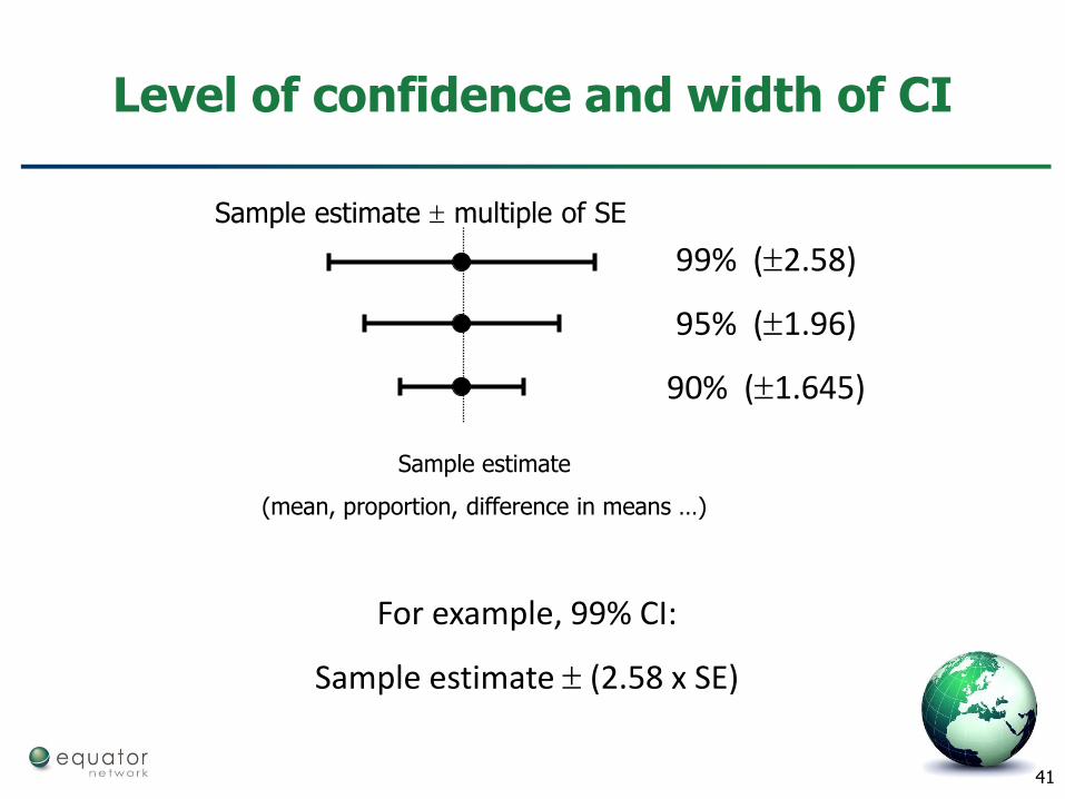
Level of confidence and width of CI

Sample estimate multiple of SE

99% (2.58)

95% (1.96)

90% (1.645)

Sample estimate

(mean, proportion, difference in means …)

For example, 99% CI:

Sample estimate (2.58 x SE)

42

Many samples

Suppose we had many samples and constructed 95% CIs from each sample

– 95% of the CIs would include the population value

43

Mean serum albumin (and 95% CI) of 100 samples (sorted by magnitude)

About 5% of confidence

intervals will not contain

the true value

Mean=33.7; SD=4.98SE=4.98/√100=0.498

95% CI 33.7±(2*0.498)[32.7, 34.7]

44

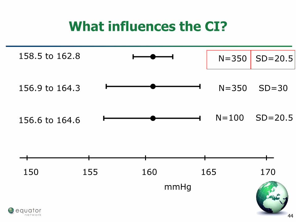
What influences the CI?

150 155 160 165 170

mmHg

N=350 SD=20.5158.5 to 162.8

N=350 SD=30156.9 to 164.3

N=100 SD=20.5156.6 to 164.6

45

Hypothesis testing: General principles

1. Set up “null hypothesis” of no effect

– e.g. active and control treatments are equally effective

2. Conduct the study

3. Calculate a “test statistic”

4. Calculate probability of the data (or more unlikely data) if the null hypothesis is true

– i.e. “P value”

– A result with P<0.05 (i.e. P<5%) is usually called (statistically) ‘significant’

46

Test statistic

The test statistic compares observed value of interest (e.g. difference between two means) with value expected under null hypothesis

For most tests the expected value of test statistic is zero – e.g. difference between 2 proportions or 2 means – so

test statistic = observed value-hypothesised value

SE of observed value

Compare test statistic to a theoretical distribution: Normal, t, 2 or F distribution to get P value

47

Mean serum albumin (and 95% CI) of 100 samples (sorted by magnitude)

Null hypothesis: mean = 35 g/l

Mean=33.7; SD=4.98SE=4.98/√100=0.498

test statistic=(33.7-35)/0.498=-2.61 P=0.01

48

Sacred 5% significance level

5% is an arbitrary level of significance

It is the probability that you would see as much (or greater) difference between the treated and control groups by chance alone

P<0.05 generally called “statistically significant”

0.05 (i.e. 5%) is an arbitrary cut-off– Is a value of p=0.046 different to 0.052?

49

Interpretation of P values

[Sterne et al. BMJ 2001]

50

Interpretation of P

P = 0.027 means that in many identical studies carried out when null hypothesis was true, we would get a result at least as extreme as this on 2.7% of occasions

Infer that null hypothesis is implausible because the data would be (very) unlikely if null hypothesis were true

– i.e. conclude that the difference is real

Clearly, the smaller the P value the more safely we may reject null hypothesis

51

P values and multiple testing

If many statistical tests have been carried out, the risk of a false positive increases

– e.g multiple outcomes, multiple time points

– Data dredging, fishing

Should take account of the multiplicity when interpreting results

Can adjust for multiple testing

– but better to think pre-specify outcomes

52

Summary

Plot your data – get a ‘feeling’ of it

Use a sample to make inferences about a population

Sample provides an estimate of an effect with some uncertainty

SE quantifies uncertainty around effect estimate

CI uses multiple of SE to indicate a range of ‘plausible’ values, assuming no bias

P value provides strength of evidence against the null hypothesis

CI and P both depend on variability and sample size

53

Useful reading

BMJ Statistics Notes (www-users.york.ac.uk/~mb55/pubs/pbstnote.htm)