data modeling
TRANSCRIPT

Data Models and Decision Making
KRISHNENDU SHAWIMT HYDERABAD

2
Let us introduce about yourself
Name Background Statistics, OR and Simulation
experiences Expectations from this course etc.

3
Learning methods PowerPoint slides-lecture Black/White board Excel based method Hand on experience on Excel, SAS etc. Mini-project Search internet Consult library Read books/magazines/newspapers Learn from your classmates/seniors
.

4
Objectives of this course… Appreciate the role of statistics in various decision
making situations
Summarize data with frequency distributions and graphic presentation.
Interpret descriptive statistics for central tendency, dispersion and location
Apply the central limit theorem to determine probabilities of sample means and compute and interpret point and interval estimates.
Utilize linear regression to estimate and predict variables.
Concept of Hypothesis testing & many more.

Introduction
We are living in the age of technology. This has two important implications for everyone entering the business world.
First, technology has made it possible to collect huge amounts of data.
Second, it has given many more people the power and responsibility to analyze data and make decisions on the basis of quantitative analysis.
A large amount of data already exists, and it will also increase in the future.

By using quantitative methods to uncover the information in the data and then acting on this information – again guided by quantitative analysis – they are able to gain advantages that their less enlightened competitors are not able to gain.

An Overview of the course
See the course outline

8
Statistics in Business
Accounting
Economics
Finance
Human resources
Marketing — market analysis and consumer research
International Business — market and demographic analysis
Operations & supply chain

Modeling and Models
A model is an abstraction of a real problem. It tries to capture the essence and key features of the problem without getting bogged down in relatively unimportant details.
There are different type of models, such as: Graphical models Algebraic models Spreadsheet models
Depending on an analyst’s preferences and skills, each can be a valuable aid in solving a real problem.

Graphical Model

Algebraic Model

Spreadsheet Model

A Seven-Step Modeling Process
1. Define the problem.2. Collect and summarize data.3. Develop a model.4. Verify the model.5. Select one or more suitable decisions.6. Present the results to the organization.7. Implement the model and update it
over time.

14
What is Statistics?
Science of gathering, analyzing, interpreting, and presenting data
Branch of mathematics Facts and figures Measurement taken on a sample Type of distribution being used to analyze data
Statistics is the scientific method that enables us to make decisions as responsibly as possible.

15
Statistics…
The science of data to answer research questions Formulate a research question
(hypothesis) Collect data Analyze and summarize data Draw conclusions to answer research
questions Statistical Inference
In the presence of variation

16
Answers Questions from Everyday Life
Business: Will a new marketing strategy be profitable?
Industry: Will a product’s life exceed the warranty period?
Medicine: Will this year’s flu vaccine reduce the chance of flu?
Education: Will technology improve learning?
Government: Will a change in interest rates affect inflation?

17
Statistics prevailing !
In Cricket (Ex: Records of centuries, wickets etc.)
In Movies (Ex: Harry Potter!)
In Media (Ex: TV serial ratings) In Stock market (Ex: Share prices)
In National Economy (Ex: WPI, Inflation, Growth, Population etc.)

18
Decision making process..
1. Collecting pertinent information that is as reliable as possible.
2. Selecting the parts of the available information that are most helpful to make rational decisions.
3. Making the actual decisions as sensibly as possible on the basis of the available evidence.
4. Perceiving the risks entailed in the particular decision made, and evaluating the corresponding risks of alternative actions.

19
Statistics: Science of variability..?
Virtually everything varies Variation occurs among individuals Variation occurs within any one individual as
time passes

20
Population Versus Sample
Population — the whole
Sample — a portion of the whole

Statistics
Descriptive Inferential

22
Data..
Secondary data : Data that has been gathered earlier for some other purpose
Sources: Company reports, GOI reports, bulletins, RBI reports, CMIE, Indiastat etc.
Primary data: Data that are collected first hand specifically for the purpose of facilitating a study
Sources: Observations, Questionnaire, Interview etc.

23
Examples of Data available from company
Employee records Name, code, designation, address, salary, leave,
Production record Item code, quantity produced, labor cost, material cost
Inventory record Item code, units-on-hand, reorder level, order quantity
Sales record Product number, volume, volume by region, category of item etc.
Customer record Age, gender, income level, address, quantity purchased

Data Sets, Variables, Observations
A data set is usually a rectangular array of data, with variables in columns and observations in rows.
A variable (or field or attribute) is a characteristic of members of a population, such as height, gender, or salary.
An observation (or case or record) is a list of all variable values for a single member of a population.


Types of Data
Numeric Discrete vs. continuous (Discrete Data can only take certain values.
For example: the number of students in a class (you can't have half a student!!!!!)
Continuous Data can take any value (within a range) For example: A person's height: could be any
value (within the range of human heights), not just certain fixed heights.
Cross-sectional vs. longitudinal
Categorical. Ordinal Nominal

Nominal - If there is no natural ordering, it is nominal.
For example: Gender (Male & Female) Hair Color (Black, blonde, brown, brunette,
red, etc).
Ordinal - If there is a natural ordering of its possible values.
For example: Economic status of the student (low, medium and high)

A dummy variable is a 0–1 coded variable for a specific category. It is coded as 1 for all observations in that category and 0 for all observations not in that category. (SPSS or Excel)
Categorizing a numerical variable as categorical is called binning (putting the data into discrete bins) or discretizing. ( For example: Range of low, Medium and High income group)
How to handle Nominal & Ordinal data ?

Assignment 1: Example 2.2: Supermarket Transactions.xlsx
Objective: To summarize categorical variables in a large data set.
Solution: Each of the counts in column S can be obtained with Excel‘s COUNTIF function.

30
Data preparation rules
Data presented must be Relevant
Before presentation always check: the source of the data that the data has been accurately transcribed the figures are relevant to the problem

Representation of the data !!!

32
Methods of visual presentation of data
How to interpret ?

Frequency Tables
A frequency table shows the number of pieces of data that fall within given intervals.

Example
Winning Score 20 34 23 34
31 35 27 49 30 52 37 20 55 20 42 39 46 38 38 27
Scores Tally Frequency
20 - 29
30 - 39
40 - 49
50 - 59
6
9
3
2
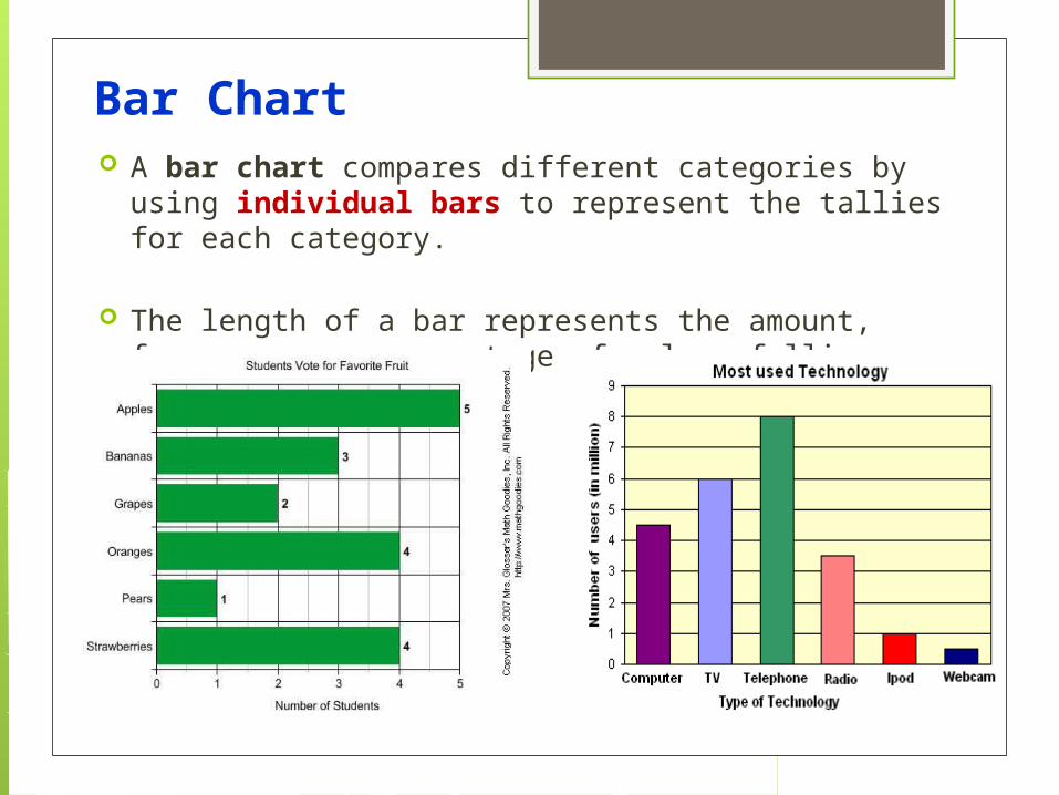
Bar Chart A bar chart compares different categories by using
individual bars to represent the tallies for each category.
The length of a bar represents the amount, frequency, or percentage of values falling into a category.

The Side-by-Side Bar Chart
A side-by-side bar chart uses sets of bars to show the joint responses from two categorical variables.

The Pie Chart
A pie chart uses parts of a circle to represent the tallies of each category. The size of each part, or pie slice, varies according to the percentage in each category.

Construct a Pie Chart

39
Ungrouped Versus Grouped Data
Ungrouped data• have not been summarized in any way• are also called raw data
Grouped data• have been organized into a frequency distribution

40
Example of Ungrouped Data
42
30
53
50
52
30
55
49
61
74
26
58
40
40
28
36
30
33
31
37
32
37
30
32
23
32
58
43
30
29
34
50
47
31
35
26
64
46
40
43
57
30
49
40
25
50
52
32
60
54
Ages of a Sample of Managers from
XYZ

41
Frequency Distribution of Ages
Class Interval Frequency20-under 30 630-under 40 1840-under 50 1150-under 60 1160-under 70 370-under 80 1
Grouped data

42
Data Range
42
30
53
50
52
30
55
49
61
74
26
58
40
40
28
36
30
33
31
37
32
37
30
32
23
32
58
43
30
29
34
50
47
31
35
26
64
46
40
43
57
30
49
40
25
50
52
32
60
54
Smallest
Largest
Range = Largest - Smallest
= 74 - 23
= 51

43
Relative Frequency
RelativeClass Interval Frequency Frequency20-under 30 6 .1230-under 40 18 .3640-under 50 11 .2250-under 60 11 .2260-under 70 3 .0670-under 80 1 .02 Total 50 1.00
6
50
18
50

44
Cumulative Frequency
CumulativeClass Interval Frequency Frequency20-under 30 6 630-under 40 18 2440-under 50 11 3550-under 60 11 4660-under 70 3 4970-under 80 1 50 Total 50
18 + 611 + 24

45
Histogram
Class IntervalFrequency20-under 30 630-under 40 1840-under 50 1150-under 60 1160-under 70 370-under 80 1
010
20
0 10 20 30 40 50 60 70 80
Years
Freq
uenc
y
A histogram is a bar chart for grouped numerical data in which you use vertical bars to represent the frequencies or percentages in each group. In a histogram, there are no gaps between adjacent bars.

46
Histogram Construction
Class Interval Frequency20-under 30 630-under 40 1840-under 50 1150-under 60 1160-under 70 370-under 80 1
010
20
0 10 20 30 40 50 60 70 80
Years
Freq
uenc
y

47
Frequency Polygon
Class Interval Frequency20-under 30 630-under 40 1840-under 50 1150-under 60 1160-under 70 370-under 80 1
010
20
0 10 20 30 40 50 60 70 80
Years
Freq
uenc
y
Frequency Polygon, a line graph is drawn by joining all the midpoints of the top of the bars of a histogram.

Example: Use of Frequency Polygon

49
Ogive
CumulativeClass Interval Frequency20-under 30 630-under 40 2440-under 50 3550-under 60 4660-under 70 4970-under 80 50 0
2040
600 10 20 30 40 50 60 70 80
Years
Freq
uenc
y

50
Relative Frequency Ogive
Cumulative
RelativeClass Interval Frequency20-under 30 .1230-under 40 .4840-under 50 .7050-under 60 .9260-under 70 .9870-under 80 1.00
0.000.100.200.300.400.500.600.700.800.901.001.10
0 10 20 30 40 50 60 70 80
YearsC
um
ula
tiv
e R
ela
tiv
e F
req
ue
nc
y

Example of Ogive
Around 85 percent students have marks in the range of 60.

52
Scatter Plot
Registered Vehicles (1000's)
Petrol Sales (1000's of
Litres)
5 60
15 120
9 90
15 140
7 60
0
100
200
0 5 10 15 20Registered Vehicles
Gas
olin
e Sa
les
Scatter plot: can explore the possible relationship between those measurements by plotting the data of one numerical variable on the horizontal, or X, axis and the data of a second numerical variable on the vertical, or Y, axis.

The Time-Series Plot

Thank you