Data Mining: Data Preprocessing

I211: Information infrastructure II

What is Data?

Collection of data objects and their attributes

Attributes

An attribute is a property or characteristic of an object

E l l f

Tid Refund Marital Status

Taxable Income Cheat

1 Yes Single 125K No– Examples: eye color of a

person, temperature, etc.– Attribute is also known as

variable field characteristic

g

2 No Married 100K No

3 No Single 70K No

4 Yes Married 120K No variable, field, characteristic, or feature

A collection of attributes

5 No Divorced 95K Yes

6 No Married 60K No

7 Yes Divorced 220K No

Objects

A collection of attributes describe an object

– Object is also known as record point case sample

8 No Single 85K Yes

9 No Married 75K No

10 No Single 90K Yes 10 record, point, case, sample,

entity, or instance

Data Preprocessingp g

Why preprocess the data?Why preprocess the data?

Descriptive data summarization (covered!)

Data cleaning

D i i d f iData integration and transformation

Data reduction

Discretization and concept hierarchy generation

Summary

Why Data Preprocessing?y p g

Data in the real world is dirtyi l t l ki tt ib t l l ki t i– incomplete: lacking attribute values, lacking certain attributes of interest, or containing only aggregate data

e.g., occupation=“ ”– noisy: containing errors or outliers

e g Salary=“-10”e.g., Salary 10– inconsistent: containing discrepancies in codes or

namesA “42” Bi thd “03/07/1997”e.g., Age=“42” Birthday=“03/07/1997”

e.g., Was rating “1,2,3”, now rating “A, B, C”e.g., discrepancy between duplicate records

Why Is Data Dirty?

Incomplete data may come from“N t li bl ” d t l h ll t d– “Not applicable” data value when collected

– Different considerations between the time when the data was collected and when it is analyzed.H /h d / ft bl– Human/hardware/software problems

Noisy data (incorrect values) may come from– Faulty data collection instruments– Human or computer error at data entry– Errors in data transmission

Inconsistent data may come fromInconsistent data may come from– Different data sources– Functional dependency violation (e.g., modify some linked data)

Duplicate records also need data cleaning

Why Is Data Preprocessing Important?

No quality data, no quality mining results!– Quality decisions must be based on quality data

e.g., duplicate or missing data may cause incorrect or even misleading statisticsmisleading statistics.

– Data warehouse needs consistent integration of quality data

Data extraction, cleaning, and transformation comprises , g, pthe majority of the work of building a data mining system

Multi-Dimensional Measure of Data Quality

A well-accepted multidimensional view:p– Accuracy– Completeness– ConsistencyConsistency– Timeliness– Believability

V l dd d– Value added– Interpretability– Accessibility

Major Tasks in Data Preprocessing

Data cleaningFill i i i l th i d t id tif tli– Fill in missing values, smooth noisy data, identify or remove outliers, and resolve inconsistencies

Data integration– Integration of multiple databases or files

Data transformation– Normalization and aggregationNormalization and aggregation

Data reduction– Obtains reduced representation in volume but produces the same or

i il l ti l ltsimilar analytical results

Data discretization– Part of data reduction but with particular importance, especially for p p , p y

numerical data

Forms of Data Preprocessing

Data Preprocessing

Why preprocess the data?Why preprocess the data?

Descriptive data summarization (covered!)

Data cleaning

D i i d f iData integration and transformation

Data reduction

Discretization and concept hierarchy generation

Summary

Data Cleaning

Importancep– garbage in garbage out principle (GIGO)

Data cleaning tasks

– Fill in missing valuesFill in missing values

– Identify outliers and smooth out noisy data

Correct inconsistent data– Correct inconsistent data

– Resolve redundancy caused by data integration

Missing Data

Data is not always available– E.g., many tuples have no recorded value for several attributes, such

as customer income in sales data

Missing data may be due toMissing data may be due to – equipment malfunction

– inconsistent with other recorded data and thus deleted

– data not entered due to misunderstanding

– certain data may not be considered important at the time of entry

– not register history or changes of the data

Missing data may need to be inferred

How to Handle Missing Data?

Ignore the tuple: usually done when class label is missing (assuming

the tasks in classification not effective when the percentage ofthe tasks in classification—not effective when the percentage of

missing values per attribute varies considerably.

Fill in the missing value manually: tedious + infeasible?Fill in the missing value manually: tedious + infeasible?

Fill in it automatically with

a global constant : e g “unknown” a new class?!– a global constant : e.g., unknown , a new class?!

– the attribute mean

– the attribute mean for all data points belonging to the same class:the attribute mean for all data points belonging to the same class:

smarter

– the most probable value: inference-based such as Bayesian formula or

decision tree

Noisy Data

Noise: random error or variance in a measured variableI t tt ib t l d tIncorrect attribute values may due to

– faulty data collection instruments– data entry problemsdata entry problems– data transmission problems– technology limitation– inconsistency in naming convention

Class label noise is hard to deal with– sometimes we don’t know whether the class label is correct or it issometimes we don t know whether the class label is correct or it is

simply unexpected

Noise demands robustness in training algorithms, that is, t i i h ld t b iti t itraining should not be sensitive to noise

How to Handle Noisy Data?

Binningfi t t d t d titi i t ( l f ) bi– first sort data and partition into (equal-frequency) bins

– then one can smooth by bin means, smooth by bin median, smooth by bin boundaries, etc.

Regression– smooth by fitting the data into regression functions

Cl t iClustering– detect and remove outliers

Combined computer and human inspectionCombined computer and human inspection– detect suspicious values and check by human (e.g., deal with

possible outliers)

Simple Discretization Methods: Binning

Equal-width (distance) partitioning

– Divides the range into N intervals of equal size: uniform grid

– if A and B are the lowest and highest values of the attribute, the width of

intervals will be: W = (B A)/Nintervals will be: W = (B –A)/N.

– The most straightforward, but outliers may dominate presentation

– Skewed data is not handled wellSkewed data is not handled well

Equal-depth (frequency) partitioning

– Divides the range into N intervals each containing approximately same– Divides the range into N intervals, each containing approximately same

number of data points

– Good data scalingg

– Managing categorical attributes can be tricky

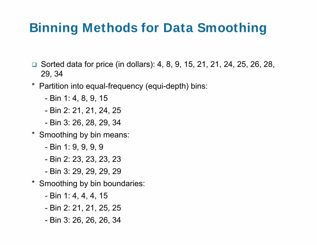
Binning Methods for Data Smoothing

Sorted data for price (in dollars): 4, 8, 9, 15, 21, 21, 24, 25, 26, 28, 29, 3429, 34

* Partition into equal-frequency (equi-depth) bins:- Bin 1: 4, 8, 9, 15- Bin 2: 21, 21, 24, 25- Bin 3: 26, 28, 29, 34

* Smoothing by bin means:g y- Bin 1: 9, 9, 9, 9- Bin 2: 23, 23, 23, 23

Bi 3 29 29 29 29- Bin 3: 29, 29, 29, 29* Smoothing by bin boundaries:

- Bin 1: 4, 4, 4, 15- Bin 2: 21, 21, 25, 25- Bin 3: 26, 26, 26, 34

Cluster Analysis as Binning

Data Cleaning as a Process

Data discrepancy detection– Use metadata (e.g., domain, range, dependency, distribution)– Check field overloading – Check uniqueness rule, consecutive rule and null rule– Use commercial tools

Data scrubbing: use simple domain knowledge (e.g., postal code, spell-check) to detect errors and make corrections

Data auditing: by analyzing data to discover rules and relationship to detect violators (e g correlation and clustering to find outliers)detect violators (e.g., correlation and clustering to find outliers)

Data migration and integration– Data migration tools: allow transformations to be specified

ETL (Extraction/Transformation/Loading) tools: allow users to specify– ETL (Extraction/Transformation/Loading) tools: allow users to specify transformations through a graphical user interface

Integration of the two processes– Iterative and interactive (e g Potter’s Wheels)– Iterative and interactive (e.g., Potter s Wheels)

Data Preprocessing

Why preprocess the data?

Data cleaning

Data integration and transformationData integration and transformation

Data reduction

Discretization and concept hierarchy generation

Summary

Data Integration

Data integration: – Combines data from multiple sources into a coherent storeCombines data from multiple sources into a coherent store

Schema integration: e.g., A.cust-id ≡ B.cust-#– Integrate metadata from different sources

E tit id tifi ti blEntity identification problem: – Identify real world entities from multiple data sources, e.g., Bill

Clinton = William ClintonDetecting and resolving data value conflicts

– For the same real world entity, attribute values from different sources are different

– Possible reasons: different representations, different scales, e.g., metric vs. British units

Handling Redundancy in Data Integration

Redundant data occur often when integration of multiple databasesdatabases

– Object identification: The same attribute or object may have different names in different databases

– Derivable data: One attribute may be a “derived” attribute in another table, e.g., annual revenue

Redundant attributes may be able to be detected byRedundant attributes may be able to be detected by correlation analysisCareful integration of the data from multiple sources mayCareful integration of the data from multiple sources may help reduce/avoid redundancies and inconsistencies and improve mining speed and quality

Correlation Analysis (Numerical Data)

Correlation coefficient (Pearson’s correlation coefficient)

nBAnAB

nBBAA

r BA σσσσ )1()(

)1())((

,

−=

−−= ∑∑

where n is the number of tuples, and are the respective means of Aand B σ and σ are the respective standard deviation of A and B and

BABA nn σσσσ )1()1( −−

A Band B, σA and σB are the respective standard deviation of A and B, and Σ(AB) is the sum of the AB cross-product.

If rA,B > 0, A and B are positively correlated (A’s values increase as B’s). The higher, the stronger correlation.rA,B = 0: uncorrelated; rA,B < 0: negatively correlated

Correlation Analysis (Categorical Data)

Χ2 (chi-square) test

n E dOb d 2)(

i th b f ibl l

∑=

−−

=n

i i

iin Expected

ExpectedObserved1

22

1)(χ

n is the number of possible valuesThe larger the Χ2 value, the more likely the variables are relatedThe cells that contribute the most to the Χ2 value are those whoseThe cells that contribute the most to the Χ value are those whose actual count is very different from the expected countCorrelation does not imply causality

– # of hospitals and # of car-theft in a city are correlated

– Both are causally linked to the third variable: population

Chi-Square Calculation: An Example

Play chess Not play chess Sum (row)

Like science fiction 250 200 450

Not like science fiction 50 1000 1050

Sum (col ) 300 1200 1500Sum (col.) 300 1200 1500

Probability to play chess: P(chess) = 300/1500 = 0.2

Probability to like science fiction: P(SciFi) = 450/1500 = 0.3

If science fiction and chess playing are independent attributes, then the probability to like SciFi AND play chess isprobability to like SciFi AND play chess is

P(SciFi, chess) = P(SciFi) · P(chess) = 0.06

That means, we expect 0.06 · 1500 = 90 such cases (if they are independent)

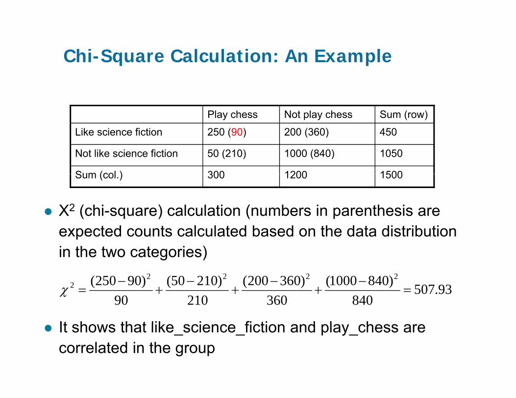
Chi-Square Calculation: An Example

Play chess Not play chess Sum (row)

Like science fiction 250 (90) 200 (360) 450

Not like science fiction 50 (210) 1000 (840) 1050

Sum (col ) 300 1200 1500

Χ2 (chi-square) calculation (numbers in parenthesis are

Sum (col.) 300 1200 1500

expected counts calculated based on the data distribution in the two categories)

2222

It shows that like science fiction and play chess are

93.507840

)8401000(360

)360200(210

)21050(90

)90250( 22222 =

−+

−+

−+

−=χ

It shows that like_science_fiction and play_chess are correlated in the group

Data Transformation

Smoothing: remove noise from dataAggregation: summarizationAggregation: summarizationGeneralization: concept hierarchy climbingNormalization: scaled to fall within a small specifiedNormalization: scaled to fall within a small, specified range

– min-max normalization– z-score normalization– normalization by decimal scaling

Attribute/feature construction– New attributes constructed from the given ones

Aggregation

Variation of Precipitation in Australia

Standard Deviation of Average Standard Deviation of Average Sta da d e at o o e ageMonthly Precipitation

Sta da d e at o o e ageYearly Precipitation

Attribute Transformation

A function that maps the entire set of values of a given attribute to a new set of replacement values gsuch that each old value can be identified with one of the new values– Simple functions: xk, log(x), ex, |x|– Standardization and Normalization

Attribute Normalization

Min-max normalization: to [new_minA, new_maxA]

i

– Ex. Let income range $12,000 to $98,000 normalized to [0.0, 1.0].

AAA

AA

A minnewminnewmaxnewminmax

minvv _)__(' +−−

−=

Then $73,000 is mapped to

716.00)00.1(000,12000,98000,12600,73

=+−−−

Z-score normalization (μ: mean, σ: standard deviation):

v μ

– Ex. Let μ = 54,000, σ = 16,000. Then

A

Avvσμ−

='

225.1000,16

000,54600,73=

−

Data Preprocessing

Why preprocess the data?Why preprocess the data?

Data cleaning

Data integration and transformation

D d iData reduction

Discretization and concept hierarchy generationp y g

Summary

Data Reduction Strategies

Why data reduction?– A database may store terabytes of data– A database may store terabytes of data– Complex data analysis/mining may take a very long time to run on the

complete data setData reductionData reduction

– Obtain a reduced representation of the data set that is much smaller in volume but yet produce the same (or almost the same) analytical resultsresults

Data reduction strategies– Data Compression

S li– Sampling– Discretization and concept hierarchy generation– Dimensionality reduction — e.g. remove unimportant attributes

Data Compression

String compressionTh t i th i d ll t d l ith– There are extensive theories and well-tuned algorithms

– Typically lossless– But only limited manipulation is possible without expansion

Audio/video compression– Typically lossy compression, with progressive refinement– Sometimes small fragments of signal can be reconstructed without

reconstructing the whole

Time sequence is not audioq– Typically short and vary slowly with time

Data Compression

Original Data Compressed Data

losslesslossless

Original DataApproximatedApproximated

Data Compression (via PCA)

Dimensions = 10Dimensions = 40Dimensions = 80Dimensions = 120Dimensions = 160Dimensions = 206

Data Reduction Method: Samplingp g

Sampling: obtaining a small sample s to represent the whole data set Nthe whole data set NAllow a mining algorithm to run in complexity that is potentially sub-linear to the size of the datais potentially sub linear to the size of the dataChoose a representative subset of the data– Simple random sampling may have very poor p p g y y p

performance in the presence of skewDevelop adaptive sampling methods

St tifi d li– Stratified sampling: Approximate the percentage of each class (or

subpopulation of interest) in the overall database p p )Used in conjunction with skewed data

Types of Sampling

Simple Random Sampling– There is an equal probability of selecting any particular item

Sampling without replacement– As each item is selected, it is removed from the populationp p

Sampling with replacement– Objects are not removed from the population as they areObjects are not removed from the population as they are

selected for the sample. In sampling with replacement, the same object can be picked up

more than once

Stratified sampling– Split the data into several partitions; then draw random samplesSplit the data into several partitions; then draw random samples

from each partition

Sampling: with or without Replacement

Raw Data

Sample Size

8000 points 2000 Points 500 Points

Sample Size

What sample size is necessary to get at least oneobject from each of 10 groups.

Sampling: Cluster or Stratified Sampling

Raw Data Cluster/Stratified Sample

Feature Subset Selection

Another way to reduce dimensionality of data

Redundant features – duplicate much or all of the information contained in

one or more other attributesone or more other attributes– Example: purchase price of a product and the amount

of sales tax paid

Irrelevant featurescontain no information that is useful for the data– contain no information that is useful for the data mining task at hand

– Example: students' ID is often irrelevant to the task of predicting students' GPA

Feature Subset Selection

Techniques:– Brute-force approach:Brute force approach:

Try all possible feature subsets as input to data mining algorithm

– Embedded approaches:Feature selection occurs naturally as part of the data mining

algorithm

– Filter approaches:Filter approaches:Features are selected before data mining algorithm is run

– Wrapper approaches:Use the data mining algorithm as a black box to find best subset

of attributes

Feature Creation

Create new attributes that can capture the important information in a data set much moreimportant information in a data set much more efficiently than the original attributes

Methodologies:– Mapping Data to New Space

Feature construction by combining features

Data Preprocessingp g

Why preprocess the data?

Data cleaning

D t i t ti d t f tiData integration and transformation

Data reduction

Discretization and concept hierarchy generation

Summary

Discretization

Three types of attributes:

– Nominal — values from an unordered set, e.g., color, professionNominal values from an unordered set, e.g., color, profession

– Ordinal — values from an ordered set, e.g., military or academic rank

– Continuous — real numbers, e.g., integer or real numbers (here we g g (

aggregated interval and ratio attributes into continuous)

Discretization:

– Divide the range of a continuous attribute into intervals

– Some classification algorithms only accept categorical attributes.

– Reduce data size by discretization

– Prepare for further analysis

Discretization Using Class Labels

Entropy based approach

3 categories for both x and y 5 categories for both x and y3 categories for both x and y 5 categories for both x and y

Discretization Without Using Class Labels

D t E l i t l idthData Equal interval width

Equal frequency K-means

Discretization and Concept Hierarchy

Discretization

– Reduce the number of values for a given continuous attribute by dividing the range of the attribute into intervals

– Interval labels can then be used to replace actual data valuesInterval labels can then be used to replace actual data values

– Supervised vs. unsupervised (use class or don’t use class variable)

– Split (top-down) vs. merge (bottom-up)

Concept hierarchy formation

– Recursively reduce the data by collecting and replacing low level concepts (such as numeric values for age) by higher level concepts (such as young, middle-aged, or senior)middle aged, or senior)

Discretization and Concept Hierarchy Generation for Numeric DataGeneration for Numeric Data

Typical methods: All the methods can be applied recursively

– Binning (covered earlier)

Top-down split, unsupervised,

– Histogram analysis (covered earlier)

Top-down split, unsupervised

Cl t i l i ( d li d i d t il l t )– Clustering analysis (covered earlier and in more detail later)

Either top-down split or bottom-up merge, unsupervised

Entropy based discretization: supervised top down split– Entropy-based discretization: supervised, top-down split

– Interval merging by χ2 Analysis: unsupervised, bottom-up merge

– Segmentation by natural partitioning: top-down split unsupervisedSegmentation by natural partitioning: top down split, unsupervised

Concept Hierarchy Generation for Categorical Data

Specification of a partial/total ordering of attributes e plicitl at the schema le el b sers or e pertsexplicitly at the schema level by users or experts

– street < city < state < country

Specification of a hierarchy for a set of values by explicitSpecification of a hierarchy for a set of values by explicit data grouping

– {Urbana, Champaign, Chicago} < Illinois

Specification of only a partial set of attributes– E.g., only street < city, not others

Automatic generation of hierarchies (or attribute levels) by the analysis of the number of distinct values

– E.g., for a set of attributes: {street, city, state, country}

Automatic Concept Hierarchy Generation

Some hierarchies can be automatically generated based on the analysis of the number of distinct values yper attribute in the data set

– The attribute with the most distinct values is placed at the lowest level of the hierarchyy

– Exceptions, e.g., weekday, month, quarter, year

15 di ti t lcountry

province_or_ state

15 distinct values

365 distinct valuesp _ _

city 3567 distinct values

street 674,339 distinct values

Data Preprocessing

Why preprocess the data?

Data cleaning

Data integration and transformation

Data reductionData reduction

Discretization and concept hierarchy

generation

SummarySummary

Summary

Data preparation or preprocessing is a big issue for data miningg

Descriptive data summarization is need for quality data preprocessingp p g

Data preparation includes– Data cleaning and data integrationg g

– Data reduction and feature selection

– Discretization

A lot a methods have been developed but data preprocessing still an active area of research