A SAS Ins t i tu te

Best Pract ices Paper

Data Mining and the Case for Sampling

Solving Business Problems Using SAS® Enterprise Miner™ Software

Table of Contents

ABSTRACT . . . . . . . . . . . . . . . . . . . . . . . . . . . . . . . . . . . . . . . . . . . . . . . . . . . . . . . . . . . . . . . . . . . . . . .1

THE OVERABUNDANCE OF DATA . . . . . . . . . . . . . . . . . . . . . . . . . . . . . . . . . . . . . . . . . . . . . . . .2

DATA MINING AND THE BUSINESS INTELLIGENCE CYCLE . . . . . . . . . . . . . . . . . . . . . . . .2

THE SEMMA METHODOLOGY . . . . . . . . . . . . . . . . . . . . . . . . . . . . . . . . . . . . . . . . . . . . . . . . . .3HOW LARGE IS “A LARGE DATABASE?” . . . . . . . . . . . . . . . . . . . . . . . . . . . . . . . . . . . . . . . .4PROCESSING THE ENTIRE DATABASE . . . . . . . . . . . . . . . . . . . . . . . . . . . . . . . . . . . . . . . . . .4PROCESSING A SAMPLE . . . . . . . . . . . . . . . . . . . . . . . . . . . . . . . . . . . . . . . . . . . . . . . . . . . . . . .6

THE STATISTICAL VALIDITY OF SAMPLING . . . . . . . . . . . . . . . . . . . . . . . . . . . . . . . . . . . . . . .8

SIZE AND QUALITY DETERMINE THE VALIDITY OF A SAMPLE . . . . . . . . . . . . . . . . .9RANDOMNESS: THE KEY TO QUALITY SAMPLES . . . . . . . . . . . . . . . . . . . . . . . . . . . . . .10CURRENT USES OF SAMPLING . . . . . . . . . . . . . . . . . . . . . . . . . . . . . . . . . . . . . . . . . . . . . . . .12WHEN SAMPLING SHOULD NOT BE USED . . . . . . . . . . . . . . . . . . . . . . . . . . . . . . . . . . . . .13MYTHS ABOUT SAMPLING . . . . . . . . . . . . . . . . . . . . . . . . . . . . . . . . . . . . . . . . . . . . . . . . . . . .13

SAMPLING AS A BEST PRACTICE IN DATA MINING . . . . . . . . . . . . . . . . . . . . . . . . . . . . . . .16

PREPARING THE DATA FOR SAMPLING . . . . . . . . . . . . . . . . . . . . . . . . . . . . . . . . . . . . . . .17COMMON TYPES OF SAMPLING . . . . . . . . . . . . . . . . . . . . . . . . . . . . . . . . . . . . . . . . . . . . . . .17DETERMINING THE SAMPLE SIZE . . . . . . . . . . . . . . . . . . . . . . . . . . . . . . . . . . . . . . . . . . . . .18GENERAL SAMPLING STRATEGIES . . . . . . . . . . . . . . . . . . . . . . . . . . . . . . . . . . . . . . . . . . . .20USING SAMPLE DATA FOR TRAINING, VALIDATION, AND TESTING . . . . . . . . . . . .21SAMPLING AND SMALL DATA TABLES . . . . . . . . . . . . . . . . . . . . . . . . . . . . . . . . . . . . . . . .21

CASE STUDY: USING SAMPLING IN CHURN ANALYSIS . . . . . . . . . . . . . . . . . . . . . . . . . . . .21

STEP 1: ACCESS THE DATA . . . . . . . . . . . . . . . . . . . . . . . . . . . . . . . . . . . . . . . . . . . . . . . . . . . .23STEP 2: SAMPLE THE DATA . . . . . . . . . . . . . . . . . . . . . . . . . . . . . . . . . . . . . . . . . . . . . . . . . . . .24STEP 3: PARTITION THE DATA . . . . . . . . . . . . . . . . . . . . . . . . . . . . . . . . . . . . . . . . . . . . . . . . .28STEP 4: DEVELOP A MODEL . . . . . . . . . . . . . . . . . . . . . . . . . . . . . . . . . . . . . . . . . . . . . . . . . . .28STEP 5: ASSESS THE RESULTS . . . . . . . . . . . . . . . . . . . . . . . . . . . . . . . . . . . . . . . . . . . . . . . . . .29SUMMARY OF CASE STUDY RESULTS . . . . . . . . . . . . . . . . . . . . . . . . . . . . . . . . . . . . . . . . . .32

SAS INSTITUTE: A LEADER IN DATA MINING SOLUTIONS . . . . . . . . . . . . . . . . . . . . . . . .33

REFERENCES . . . . . . . . . . . . . . . . . . . . . . . . . . . . . . . . . . . . . . . . . . . . . . . . . . . . . . . . . . . . . . . . . . .34

RECOMMENDED READING . . . . . . . . . . . . . . . . . . . . . . . . . . . . . . . . . . . . . . . . . . . . . . . . . . . . .35

DATA MINING . . . . . . . . . . . . . . . . . . . . . . . . . . . . . . . . . . . . . . . . . . . . . . . . . . . . . . . . . . . . . . . .35DATA WAREHOUSING . . . . . . . . . . . . . . . . . . . . . . . . . . . . . . . . . . . . . . . . . . . . . . . . . . . . . . . .35STATISTICS . . . . . . . . . . . . . . . . . . . . . . . . . . . . . . . . . . . . . . . . . . . . . . . . . . . . . . . . . . . . . . . . . . .35

CREDITS . . . . . . . . . . . . . . . . . . . . . . . . . . . . . . . . . . . . . . . . . . . . . . . . . . . . . . . . . . . . . . . . . . . . . . . .36

i

Figures

Figure 1 : The Data Mining Process and the Business Intelligence Cycle . . . . . . . . . . . . . . . . . . . . . . .2Figure 2 : Steps in the SEMMA Methodology . . . . . . . . . . . . . . . . . . . . . . . . . . . . . . . . . . . . . . . . . . . . .3Figure 3 : How Sampling Size Affects Validity . . . . . . . . . . . . . . . . . . . . . . . . . . . . . . . . . . . . . . . . . . . . .9Figure 4 : How Samples Reveal the Distribution of Data . . . . . . . . . . . . . . . . . . . . . . . . . . . . . . . . . . .11Figure 5 : Example Surface Plots for Fitted Models; Regression, Decision Tree, and

Neural Network . . . . . . . . . . . . . . . . . . . . . . . . . . . . . . . . . . . . . . . . . . . . . . . . . . . . . . . . . . . .19Figure 6 : Churn Analysis — Steps, Actions, and Nodes . . . . . . . . . . . . . . . . . . . . . . . . . . . . . . . . . . . .22Figure 7 : Process Flow Diagram for the Customer Churn Project . . . . . . . . . . . . . . . . . . . . . . . . . . . .22Figure 8 : Input Data - Interval Variable . . . . . . . . . . . . . . . . . . . . . . . . . . . . . . . . . . . . . . . . . . . . . . . . .23Figure 9 : Input Data - Class Variables . . . . . . . . . . . . . . . . . . . . . . . . . . . . . . . . . . . . . . . . . . . . . . . . . .23Figure 10 : Percentage of Churn and No Churn . . . . . . . . . . . . . . . . . . . . . . . . . . . . . . . . . . . . . . . . . . . .24Figure 11 : General Dialog Page . . . . . . . . . . . . . . . . . . . . . . . . . . . . . . . . . . . . . . . . . . . . . . . . . . . . . . . .25Figure 12 : Stratification Variables Dialog Page . . . . . . . . . . . . . . . . . . . . . . . . . . . . . . . . . . . . . . . . . . . .26Figure 13 : Stratification Criteria Dialog Page . . . . . . . . . . . . . . . . . . . . . . . . . . . . . . . . . . . . . . . . . . . . .27Figure 14 : Sampling Results Browser . . . . . . . . . . . . . . . . . . . . . . . . . . . . . . . . . . . . . . . . . . . . . . . . . . . .27Figure 15 : Data Partition Dialog Page . . . . . . . . . . . . . . . . . . . . . . . . . . . . . . . . . . . . . . . . . . . . . . . . . . .28Figure 16 : Regression Results . . . . . . . . . . . . . . . . . . . . . . . . . . . . . . . . . . . . . . . . . . . . . . . . . . . . . . . . . .29Figure 17 : Diagnostic Chart for Validation Data . . . . . . . . . . . . . . . . . . . . . . . . . . . . . . . . . . . . . . . . . . .30Figure 18 : Diagnostic Chart for Test Data . . . . . . . . . . . . . . . . . . . . . . . . . . . . . . . . . . . . . . . . . . . . . . . .30Figure 19 : Incremental Sample Size and the Correct Classification Rates . . . . . . . . . . . . . . . . . . . . . .31Figure 20 : Comparison of Sample Sizes . . . . . . . . . . . . . . . . . . . . . . . . . . . . . . . . . . . . . . . . . . . . . . . . . .32

ii

1

1Accessing, aggregating, and transforming data are primary functions of data warehousing. For more information on data warehousing,see the “Recommended Reading” section in this paper.

2Unscrubbed data and similar terms refer to data that are not prepared for analysis. Unscrubbed data should be cleaned (scrubbed, transformed) to correct errors such as missing values, inconsistent variable names, and inconsequential outliers before being analyzed.

Abstract

Industry analysts expect the use of data mining to sustain double-digit growth into the 21stcentury. One recent study, for example, predicts the worldwide statistical and data miningsoftware market to grow at a compound annual growth rate of 16.1 percent over the nextfive years, reaching $1.13 billion in the year 2002 (International Data Corporation 1998#15932).

Many large- to mid-sized organizations in the mainstream of business, industry, and the publicsector already rely heavily on the use of data mining as a way to search for relationships thatwould otherwise be “hidden” in their transaction data. However, even with powerful datamining techniques, it is possible for relationships in data to remain hidden due to the presenceof one or more of the following conditions:

• data are not properly aggregated

• data are not prepared for analysis

• relationships in the data are too complex to be seen readily via human observation

• databases are too large to be processed economically as a whole.

All of these conditions are complex problems that present their own unique challenges. For example, organizing data by subject into data warehouses or data marts can solve problems associated with aggregation.1 Data that contain errors, missing values, or otherproblems can be cleaned in preparation for analysis.2 Relationships that are counter-intuitiveor highly complex can be revealed by applying predictive modeling techniques such as neuralnetworks, regression analysis, and decision trees as well as exploratory techniques like clustering, associations and sequencing. However, processing large databases en masse isanother story — one that carries along with it its own unique set of problems.

This paper discusses the use of sampling as a statistically valid practice for processing largedatabases by exploring the following topics:

• data mining as a part of the “Business Intelligence Cycle”

• sampling as a valid and frequently-used practice for statistical analyses

• sampling as a best practice in data mining

• a data mining case study that relies on sampling.

For those who want to study further the topics of data mining and the use of sampling to process large amounts of data, this paper also provides references and a list of recommended reading material.

The Overabundance of Data

In the past, many businesses and other organizations were unable or unwilling to store theirhistorical data. Online transaction processing (OLTP) systems, rather than decision supportsystems, were key to business. A primary reason for not storing historical data was the factthat disk space was comparatively more expensive than it is now. Even if the storage spacewas available, IT resources often could not be spared to implement and maintain enterprise-wide endeavors like decision support systems.

Times have changed. As disk storage has become increasingly affordable, businesses haverealized that their data can, in fact, be used as a corporate asset for competitive advantage. Forexample, customers’ previous buying patterns often are good predictors of their future buyingpatterns. As a result, many businesses now search their data to reveal those historical patterns.

To benefit from the assets bound up in their data, organizations have invested numerousresources to develop data warehouses and data marts. The result has been substantialreturns on these kinds of investments. However, now that affordable systems exist forstoring and organizing large amounts of data, businesses face new challenges. For example,how can hardware and software systems sift through vast warehouses of data efficiently?What process leads from data, to information, to competitive advantage?

While data storage has become cheaper, CPU, throughput, memory management, and net-work bandwidth continue to be constraints when it comes to processing large quantities ofdata. Many IT managers and business analysts are so overwhelmed with the sheer volume,they do not know where to start. Given these massive amounts of data, many ask, “How canwe even begin to move from data to information?” The answer is in a data mining processthat relies on sampling, visual representations for data exploration, statistical analysis andmodeling, and assessment of the results.

Data Mining and the Business Intelligence Cycle

During 1995, SAS Institute Inc. began research, development, and testing of a data miningsolution based on our world-renowned statistical analysis and reporting software — the SAS System. That work, which resulted in the 1998 release of SAS Enterprise Miner™ soft-ware, taught us some important lessons.3 One lesson we learned is that data mining is aprocess that must itself be integrated within the larger process of business intelligence. Figure 1 illustrates the role data mining plays in the business intelligence cycle.

Integrating data mining activities with the organiza-tion’s data warehouse and business reporting systemsenables the technology to fit within the existing IT infrastructure while supporting the organization’s larger goals of

• identifying business problems,

• transforming data into information,

• acting on the information, and

• assessing the results.

Figure 1 : The Data Mining Process and the Business Intelligence Cycle

2

3According to the META Group, “The SAS Data Mining approach provides an end-to-end solution, in both the sense of integratingdata mining into the SAS Data Warehouse, and in supporting the data mining process. Here, SAS is the leader” (META Group 1997, file #594).

BusinessQuestions

Data WarehouseDBMS

Data MiningProcess

EIS, BusinessReportingGraphics

IdentifyProblem

Act on Infor-mation

TransformData Into

InformationMeasureResults

The SEMMA MethodologySAS Institute defines data mining as the process used to reveal valuable information and complex relationships that exist in large amounts of data. Data mining is an iterative process —answers to one set of questions often lead to more interesting and more specific questions.To provide a methodology in which the process can operate, SAS Institute further dividesdata mining into five stages that are represented by the acronym SEMMA.

Beginning with a statistically representative sample of data, the SEMMA methodology —which stands for Sample, Explore, Modify, Model, and Assess — makes it easy for businessanalysts to apply exploratory statistical and visualization techniques, select and transformthe most significant predictive variables, model the variables to predict outcomes, and confirma model’s accuracy. Here is an overview of each step in the SEMMA methodology:

• Sample the data by creating one or more data tables.4 The samples should be bigenough to contain the significant information, yet small enough to process quickly.

• Explore the data by searching for anticipated relationships, unanticipated trends, andanomalies in order to gain understanding and ideas.

• Modify the data by creating, selecting, and transforming the variables to focus the modelselection process.

• Model the data by allowing the software to search automatically for a combination ofdata that reliably predicts a desired outcome.

• Assess the data by evaluating the usefulness and reliability of the findings from the datamining process.

SEMMA is itself a cycle; the internal steps can be performed iteratively as needed. Figure 2illustrates the tasks of a data mining project and maps those tasks to the five stages of theSEMMA methodology. Projects that follow SEMMA can sift through millions of records5

and reveal patterns that enable businesses to meet data mining objectives such as:

• Segmenting customers accurately intogroups with similar buying patterns

• Profiling customers for individual relationship management

• Dramatically increasing response rate fromdirect mail campaigns

• Identifying the most profitable customersand the underlying reasons

• Understanding why customers leave forcompetitors (attrition, churn analysis)

• Uncovering factors affecting purchasingpatterns, payments and response rates

• Increasing profits by marketing to thosemost likely to purchase

3

4The terms data table and data set are synonymous.

5Record refers to an entire row of data in a data table. Synonyms for the term record include observation, case, and event. Row refers to the way data are arranged horizontally in a data table structure.

Figure 2 : Steps in the SEMMA Methodology

• Decreasing costs by filtering out those least likely to purchase

• Detecting patterns to uncover non-compliance.

How Large is “A Large Database”To find patterns in data such as identifying the most profitable customers and the underlyingreasons for their profitability, a solution must be able to process large amounts of data.However, defining “large” is like trying to hit a moving target; the definition of “a largedatabase” is changing as fast as the enabling technology itself is changing. For example, theprefix tera, which comes from the Greek teras meaning “monster,” is used routinely to identify databases that contain approximately one trillion bytes of data. Many statisticianswould consider a database of 100,000 records to be very large, but data warehouses filledwith a terabyte or more of data such as credit card transactions with associated demograph-ics are not uncommon. Performing routine statistical analyses on even a terabyte of data canbe extremely expensive and time consuming. Perhaps the need to work with even moremassive amounts of data such as a petabyte (250) is not that far off in the future (Potts 1997, p. 10).

So what can be done when the volume of data grows to such massive proportions? Theanswer is deceptively simple; either

• try to process the entire database, or

• process only a sample of it.

Processing the Entire DatabaseTo move from massive amounts of data to business intelligence, some practitioners arguethat automated algorithms with faster and faster processing times justify processing theentire database. However, no single approach solves all data mining problems. Instead,processing the entire database offers both advantages and disadvantages depending on thedata mining project.

AdvantagesAlthough data mining often presupposes the need to process very large databases, somedata mining projects can be performed successfully when the databases are small. For example,all of the data could be processed when there are more variables6 than there are records. Insuch a situation, there are statistical techniques that can help ensure valid results in whichcase, an advantage of processing the entire database is that enough richness can be maintainedin the limited, existing data to ensure a more precise fit.

In other cases, the underlying process that generates the data may be rapidly changing, andrecords are comparable only over a relatively short time period. As the records age, theymight lose value. Older data can become essentially worthless. For example, the value ofsales transaction data associated with clothing fads is often short lived. Data generated bysuch rapidly changing processes must be analyzed often to produce even short-term forecasts.

Processing the entire database also can be advantageous in sophisticated exception reportingsystems that find anomalies in the database or highlight values above or below some thresh-old level that meet the selected criteria.

4

6Variable refers to a characteristic that defines records in a data table such as a variable B_DATE, which would contain customers’birth dates. Column refers to the way data are arranged vertically within a data table structure.

If the solution to the business problem is tied to one record or a few records, then to findthat subset, it may be optimal to process the complete database. For example, suppose a chainof retail paint stores discovers that too many customers are returning paint. Paint pigmentsused to mix the paints are obtained from several outside suppliers. Where is the problem?With retailers? With customers? With suppliers? What actions should be taken to correct theproblem? The company maintains many databases consisting of various kinds of informationabout customers, retailers, suppliers, and products. Routine anomaly detection (processingthat is designed to detect whether a summary performance measure is beyond an acceptablerange) might find that a specific store has a high percentage of returned paint. A subsequentinvestigation discovers that employees at that store mix pigments improperly. Clearerinstructions could eliminate the problem. In a case like this one, the results are definitiveand tied to a single record. If the data had been sampled for analysis, then that single,important record might not have been included in the sample.

DisadvantagesProcessing the entire database affects various aspects of the data mining process includingthe following:

Inference/GeneralizationThe goal of inference and predictive modeling is to apply successfully findings from adata mining system to new records. Data mining systems that exhaustively search thedatabases often leave no data from which to develop inferences. Processing all of thedata also leaves no holdout data with which to test the model for explanatory power onnew events. In addition, using all of the data leaves no way to validate findings on dataunseen by the model. In other words, there is no room left to accomplish the goal ofinference.

Instead, holdout samples must be available to ensure confidence in data mining results.According to Elder and Pregibon, the true goal of most empirical modeling activities is“to employ simplifying constraints alongside accuracy measures during model formula-tion in order to best generalize to new cases” (1996, p. 95).

Occasionally, concerns arise about the way sampling might affect inference. This con-cern is often expressed as a belief that a sample might miss some subtle but importantniches — those “hidden nuggets” in the database. However, if a niche is so tiny that it isnot represented in a sample and yet so important as to influence the big picture, theniche can be discovered: either by automated anomaly detection or by using appropri-ate sampling methods. If there are pockets of important information hidden in thedatabase, application of the appropriate sampling technique will reveal them and willprocess much faster than processing the whole database.

Quality of the FindingsUsing exhaustive methods when developing predictive models may actually create morework by revealing spurious relationships. For example, exhaustive searches may “dis-cover” such intuitive relationships as the fact that people with large account balancestend to have higher incomes, that residential electric power usage is low between 2 a.m.and 4 a.m., or that travel-related expenditures increase during the holidays. Spendingtime and money to arrive at such obvious conclusions can be avoided by working withmore relevant subsets of data. More findings do not necessarily mean quality findingsand sifting through the findings to determine which are valid takes time and effort.

5

In addition to unreliable forecasts, exhaustive searches tend to produce several indepen-dent findings, each of which needs a corresponding set of records on which to baseinferences. Faster search algorithms on more data can produce more findings but withless confidence in any of them.

Speed and EfficiencyPerhaps the most persistent problems concerning the processing of large databases arespeed and cost. Analytical routines required for exploration and modeling run faster onsamples than on the entire database. Even the fastest hardware and software combina-tions have difficulty performing complex analyses such as fitting a stepwise logisticregression with millions of records and hundreds of input variables. For most businessproblems, there comes a point when the time and money spent on processing the entiredatabase produces diminishing returns wherein any potential modest gains are simplynot worth the cost. In fact, even if a business were to ignore the advantages of statisticalsampling and instead choose to process data in its entirety (assuming multiple terabytesof data), no time-efficient and cost-effective hardware/software solution that excludesstatistical sampling yet exists.

Within a database, there can be huge variations across individual records. A few datavalues far from the main cluster can overly influence the analysis, and result in largerforecast errors and higher misclassification rates. These data values may have been mis-coded values, they may be old data, or they may be outlying records. Had the samplebeen taken from the main cluster, these outlying records would not have been overlyinfluential.

Alternatively, little variation might exist in the data for many of the variables; the recordsare very similar in many ways. Performing computationally intensive processing on theentire database might provide no additional information beyond what can be obtainedfrom processing a small, well-chosen sample. Moreover, when the entire database isprocessed, the benefits that might have been obtained from a pilot study are lost.

For some business problems, the analysis involves the destruction of an item. For exam-ple, to test the quality of a new automobile, it is torn apart or run until parts fail. Manyproducts are tested in this way. Typically, only a sample of a batch is analyzed using thisapproach. If the analysis involves the destruction of an item, then processing the entiredatabase is rarely viable.

Processing a Sample Corporations that have achieved significant return on investment (ROI) in data mining havedone so by performing predictive data mining. Predictive data mining requires the developmentof accurate predictive models that typically rely on sampling in one or more forms. ROI is thefinal justification for data mining, and most often, the return begins with a relatively small sample.7

AdvantagesExploring a representative sample is easier, more efficient, and can be as accurate as explor-ing the entire database. After the initial sample is explored, some preliminary models canbe fitted and assessed. If the preliminary models perform well, then perhaps the data min-ing project can continue to the next phase. However, it is likely that the initial modeling gen-erates additional, more specific questions, and more data exploration is required.

6

7Sampling also is effective when using exploratory or descriptive data mining techniques; however, the goals and benefits (and hencethe ROI) of using these techniques are less well defined.

In most cases, a database is logically a subset or a sample of some larger population.8 Forexample, a database that contains sales records must be delimited in some way such as bythe month in which the items were sold. Thus, next month’s records will represent a differ-ent sample from this month’s. The same logic would apply to longer time frames such asyears, decades, and so on. Additionally, databases can at best hold only a fraction of theinformation required to fully describe customers, suppliers, and distributors. In the extreme,the largest possible database would be all transactions of all types over the longest possibletime frame that fully describes the enterprise.

Speed and EfficiencyA major benefit of sampling is the speed and efficiency of working with a smaller datatable that still contains the essence of the entire database. Ideally, one uses enough datato reveal the important findings, and no more. Sufficient quantity depends mostly onthe modeling technique, and that in turn depends on the problem. “A sample surveycosts less than a complete enumeration, is usually less time consuming, and may evenbe more accurate than a complete enumeration,” as Saerndal, Swensson, and Wretman(1992, p. 3) point out. Sampling enables analysts to spend relatively more time fittingmodels and thereby less time waiting for modeling results.

The speed and efficiency of a process can be measured in various ways. Throughput isa common measure; however, when business intelligence is the goal, business-orientedmeasurements are more useful. In the context of business intelligence, it makes moresense to ask big picture questions about the speed and efficiency of the entire businessintelligence cycle than it does to dwell on smaller measurements that merely contributeto the whole such as query/response times or CPU cycles.

Perhaps the most encompassing business-oriented measurement is one that seeks todetermine the cost in time and money to go from the recording of transactions to a planof action. That path — from OLTP to taking action — includes formulating the businessquestions, getting the data in a form to be mined, analyzing it, evaluating and dissemi-nating the results, and finally, taking action.

VisualizationData visualization and exploration facilitate understanding of the data.9 To betterunderstand a variable, univariate plots of the distribution of values are useful. To examinerelationships among variables, bar charts and scatter plots (2-dimensional and 3-dimensional)are helpful. To understand the relationships among large numbers of variables, correlationtables are useful. However, huge quantities of data require more resources and moretime to plot and manipulate (as in rotating data cubes). Even with the many recentdevelopments in data visualization, one cannot effectively view huge quantities of datain a meaningful way. A representative sample gives visual order to the data and allowsthe analyst to gain insights that speed the modeling process.

GeneralizationSamples obtained by appropriate sampling methods are representative of the entiredatabase and therefore little (if any) information is lost. Sampling is statistically depend-able. It is a mathematical science based on the demonstrable laws of probability, uponwhich a large part of statistics is built.10

7

8Population refers to the entire collection of data from which samples are taken such as the entire database or data warehouse.

9Using data visualization techniques for exploration is Step 2 in the SEMMA process for data mining. For more information, see thesources listed for data mining in the “Recommended Reading” section of this paper.

10For more information on the statistical bases of sampling, see the section “The Statistical Validity of Sampling” in this paper.

EconomyData cleansing (detecting, investigating, and correcting errors, outliers, missing values,and so on) can be very time-consuming. To cleanse the entire database might be a verydifficult and frustrating task. To the extent that a well-designed data warehouse or martis in place, much of this cleansing has already been addressed. However, even with“clean” data in a warehouse or mart, additional pre-processing may be useful for thedata mining project. There may still be missing values or other fields that need to bemodified to address specific business problems. Business problems may require certaindata assumptions, which indicate the need for additional data preparation. For exam-ple, a missing value for DEPENDENTS actually could be missing, or the value could be“zero.” Rather than leave these values as missing, for analytical purposes, you may wantto impute a value based on the available information.

If a well-designed and well-prepared data warehouse or mart is in place, less data pre-processing is necessary. The remaining data pre-processing is performed as needed foreach specific business problem, and it is much more efficiently done on a sample.

Data augmentation (adding information to the data such as demographics, creditbureau scores, and so on), like data cleaning, will be less expensive if applied only to asample. If the analysis is complicated and computationally intensive, it may be cost-effective to run a pilot study to see if further analysis is warranted. If additional data areto be purchased to augment the currently available data, then a test study on one partof the data might be an excellent approach. For example, the additional data for onegeographic region could be purchased. Then as a pilot study, the full analysis performedon that one geographic region. After assessing the pilot study results, the decision couldbe made about purchasing additional data.11

In general, if a small-scale pilot study (based on a representative sample) provides use-ful results, then the costs of performing a larger, more comprehensive study may be aworthwhile investment. If the pilot study does not provide useful results, then it maybe better to stop this line of analysis and go to the next problem.

DisadvantagesNot all samples are created equal. To be representative, a sample should reflect the characteristics of the data. Business analysts must know the data well enough to preservethe important characteristics of the database. In addition, the technology must be robustenough to perform various sampling techniques, because different sampling techniques areappropriate in different situations.

The Statistical Validity of Sampling

Statistics is a branch of applied mathematics that enables researchers to identify relation-ships and to search for ways to understand relationships. Modern statistical methods relyon sampling. Analysts routinely use sampling techniques to run initial models, enable explo-ration of data, and determine whether more analysis is needed. Data mining techniques that

8

11SAS Institute Inc. has agreements with a number of data providers including Claritas Inc., Geographic Data Technologies, andAcxiom Corporation.

use statistical sampling methods can reveal valuable information and complex relationshipsin large amounts of data — relationships that might otherwise be hidden in a company’sdata warehouse.

Size and Quality Determine the Validity of a Sample In data mining, the sample data is used to construct predictive models, which in turn, areused to make predictions about an entire database. Therefore, the validity of a sample, thatis, whether the sample is representative of the entire database, is critically important.

Whether a sample is representative of the entire database is determined by two characteris-tics — the size of the sample and the quality of the sample. The importance of sample size isrelatively easy to understand. However, understanding the importance of quality is a bit moreinvolved, because a quality sample for one business problem may not be a quality sample foranother problem.

How the Size of Samples Affects Validity As the size of the sample grows, it should with increasing clarity reflect the patterns that arepresent in the entire database. When we compare a graphical representation of a samplewith one of a database, we readily can see how samples are able to reflect the patterns orshapes of databases.

For example, Figure 3 graphs customer income levels. Graph A represents the entire database(100 percent of the records), and reveals that most of the customers are of middle income.As you go toward the extremes — either very low or very high income levels, the numberof customer records declines. Graph B, which is a sample of 30 percent of the database,reveals the same overall pattern or shape of the database. Statisticians refer to this patternas the distribution of the data.

Figure 3 : How Sampling Size Affects Validity

If we were to increase the size of the sample, it would continue to take on the distribution ofthe database. Taken to a logical extreme, if we read the entire database, we have the largest,most comprehensive “sample” available — the database itself. The distribution would, ofcourse, be the same, and any inferences we make about that “sample” would be true for theentire database.12

9

Customers by Income Levels

low high low high

A: 100 percent B: 30 percent

12For more information about the size of samples, see the section “Sampling as a Best Practice in Data Mining: Determining the Sample Size” in this paper.

How the Quality of Samples Affects Validity Quality, in the context of statistical sampling techniques, refers to whether the sample capturesthe characteristics of the database that are needed to solve the business problem. Is thesample in fact an ideal representation of the data at large? The highest quality sample wouldbe an exact miniature of the database; it would preserve the distributions of individual variablesand the relationships among variables. At the other extreme, the lowest quality samplewould be so unrepresentative or biased in some direction as to be of no use. In practice, a sample should be unbiased enough to be at least typical of the database.

But how is it possible to construct unbiased samples? How can we ensure that the samplesused in statistical analyses such as data mining projects are representative of the entire database? The answer lies in the procedures used to select records from the database.The sampling selection procedures determine the likelihood that any given record willbe included in the sample. To construct an unbiased sample, the procedure must be basedon a proven, quantifiable selection method — one from which reliable statistics can beobtained. In the least sophisticated form of sampling, each record has the same probabilityof being selected.

Randomness: the Key to Quality SamplesThe concept of randomness and the role it plays in creating unbiased samples can be seen in a technique that is fundamental to statistical analysis. That technique is simple randomsampling. In this context, simple means that the records are selected from the database intheir “simplest form;” that is, the records are not preprocessed or grouped in some mannerprior to sampling (Phillips 1996, p. 91).

Random in this context does not mean haphazard or capricious. Instead, random refers to alack of bias in the selection method. In a random sample, each record in the database hasan equal chance of being selected for inclusion in the sample. Random sampling in a senselevels the playing field for all records in a database giving each record the same chance ofbeing chosen, and thereby ensuring that a sample of sufficient quantity will represent theoverall pattern of the database. For example, to create a simple random sample from acustomer database of one million records, you could use a selection process that wouldassign numbers to all of the records — one through one million. Then the selection processcould randomly select numbers (Hays 1973, pp. 20-22).

Random Samples Reveal the Distribution of the DataWhen we randomly select records from a database and obtain a sample of sufficient size, thesample reflects characteristics of the database as a whole. As shown previously in Figure 3,as the sample size gets larger, the distribution (shape) of the sample reflects the distributionof the entire database. In Figure 3, the data have a symmetric and bell-shaped distribution.This is a commonly occurring and well-understood type of shape and is referred to as anormal distribution.

Not all data are distributed normally. Graphical representations of databases often revealthat the data are skewed in one direction or the other. For example, if in Figure 3, most ofthe customers had relatively lower incomes, then the distribution would be skewed to theright. If these data were randomly sampled, then as the sample size gets larger, its distributionwould reflect better the distribution of the entire database.

10

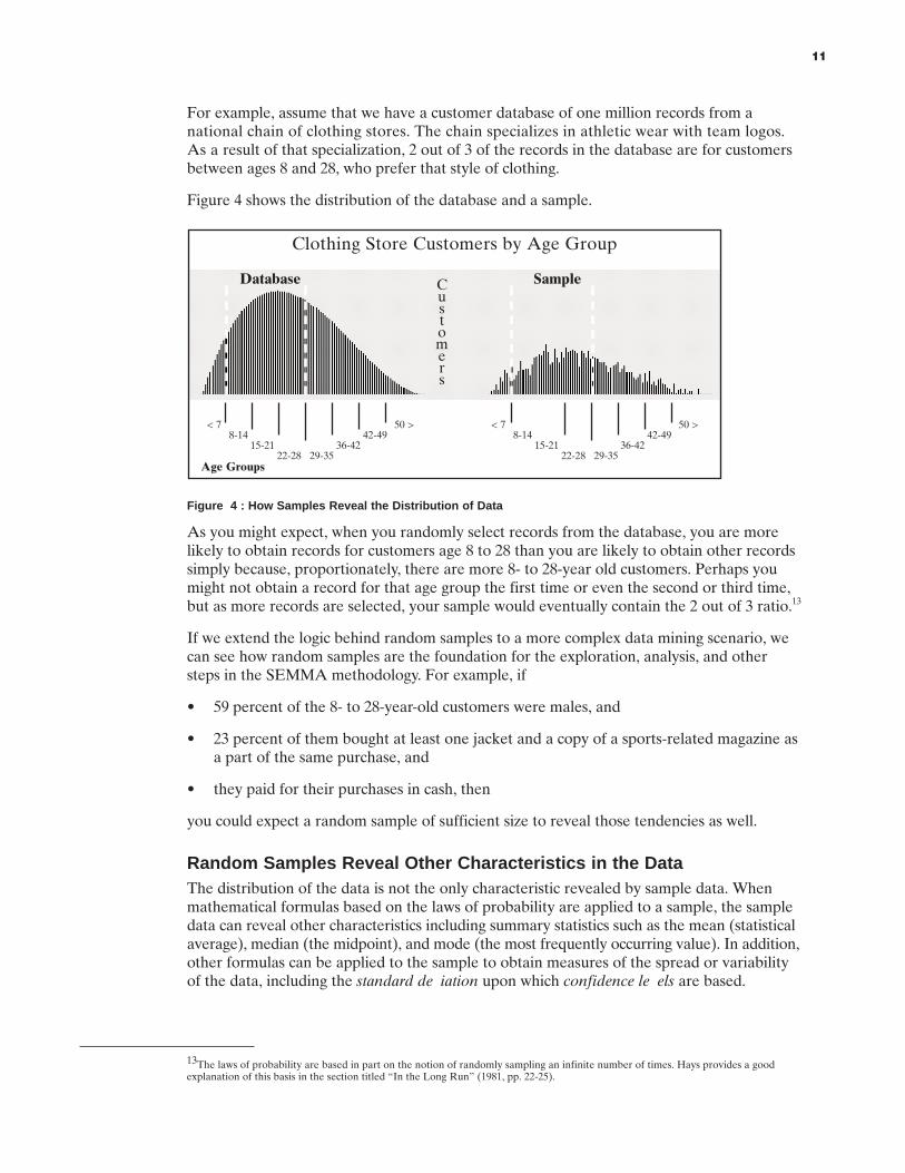
For example, assume that we have a customer database of one million records from anational chain of clothing stores. The chain specializes in athletic wear with team logos.As a result of that specialization, 2 out of 3 of the records in the database are for customersbetween ages 8 and 28, who prefer that style of clothing.

Figure 4 shows the distribution of the database and a sample.

Figure 4 : How Samples Reveal the Distribution of Data

As you might expect, when you randomly select records from the database, you are morelikely to obtain records for customers age 8 to 28 than you are likely to obtain other recordssimply because, proportionately, there are more 8- to 28-year old customers. Perhaps youmight not obtain a record for that age group the first time or even the second or third time,but as more records are selected, your sample would eventually contain the 2 out of 3 ratio.13

If we extend the logic behind random samples to a more complex data mining scenario, wecan see how random samples are the foundation for the exploration, analysis, and othersteps in the SEMMA methodology. For example, if

• 59 percent of the 8- to 28-year-old customers were males, and

• 23 percent of them bought at least one jacket and a copy of a sports-related magazine asa part of the same purchase, and

• they paid for their purchases in cash, then

you could expect a random sample of sufficient size to reveal those tendencies as well.

Random Samples Reveal Other Characteristics in the DataThe distribution of the data is not the only characteristic revealed by sample data. Whenmathematical formulas based on the laws of probability are applied to a sample, the sampledata can reveal other characteristics including summary statistics such as the mean (statisticalaverage), median (the midpoint), and mode (the most frequently occurring value). In addition,other formulas can be applied to the sample to obtain measures of the spread or variabilityof the data, including the standard deviation upon which confidence levels are based.

11

Clothing Store Customers by Age Group

Age Groups

< 78-14

15-2122-28 29-35

36-4242-49

50 > < 78-14

15-2122-28 29-35

36-4242-49

50 >

Database SampleCustomers

13The laws of probability are based in part on the notion of randomly sampling an infinite number of times. Hays provides a goodexplanation of this basis in the section titled “In the Long Run” (1981, pp. 22-25).

Stated simply, standard deviation is the average distance of the data from the mean. Confidencelevel refers to the percentage of records that are within a specified number of standarddeviations from the mean value. For a normal (symmetric, bell-shaped) distribution, approx-imately 68 percent of all records in a database will fall within a range that is 1 standarddeviation above and below the mean. Approximately 95 percent of all records will fallwithin a range that is 2 standard deviations above and below the mean (Hays 1981, p. 209).

In summary, when we have a database and use an unbiased selection process to obtain records,then at some point as more and more records are selected, the sample will reveal the distrib-ution of the database itself. In addition, by applying mathematical formulas based on laws ofprobability, we can determine other characteristics of the entire database. These samplingtechniques and their underlying principles hold true for all populations regardless of the particular application. It does not matter whether we are rolling dice, blindly pulling red andwhite marbles from a barrel, or randomly selecting records from a year’s worth of customertransaction data in order to construct a sample data table for use in a data mining project.14

Current Uses of SamplingSampling has grown into a universally accepted approach for gathering information, and it iswidely accepted that a fairly modest-sized sample can sufficiently characterize a much largerpopulation. Sampling is used extensively by governments to identify problem areas andnational trends, as well as to measure their scope and scale. For example, sampling is usedin the United States to measure and to characterize unemployment and the size of the laborforce, industrial production, wholesale and retail prices, population health statistics, familyincomes and expenditures, and agricultural production and land use. As Cochran (1977, p. 3)points out in Sampling Techniques, sampling associated with the U.S. national census wasintroduced in 1940 and its use in survey questions has grown steadily:

Except for certain basic information required for every person for constitutionalor legal reasons, the whole census was shifted to a sample basis. This change,accompanied by greatly increased mechanization, resulted in much earlier publication and substantial savings.

Today, the U.S. government publishes numerous reports based on sample data obtainedduring censuses. For example, sampling conducted during the 1990 census was used as thebasis for a variety of reports that trace statistics relating to social, labor, income, housing,and poverty (U.S. Bureau of the Census 1992).

Sampling is also used by local governments and by commercial firms. Television and radiobroadcasters constantly monitor audience sizes. Marketing firms strive to know customerreactions to new products and new packaging. Manufacturing firms make decisions toaccept or reject whole batches of a product based on the sample results. Public opinion and elections polls have used sampling techniques for decades.

Sampling of an “untreated” group can provide a baseline for comparing the “treated” group,and hence for assessing the effectiveness of the treatment. Researchers in various fieldsroutinely conduct studies that examine wide-ranging topics including human behavior andhealth; sampling is often an integral part of these analyses.

12

14The techniques used in sampling (and the mathematical formulas that statisticians use to express those techniques) grew out of thestudy of probability. The laws of probability grew out of the study of gambling — in particular, the work of the 17th century mathemati-cians Blaise Pascal and Pierre de Fermat who formulated the mathematics of probability by observing the odds associated with rollingdice. Their work is the basis of the theory of probability in its modern form (Ross 1998, p. 89).

When Sampling Should Not Be UsedSampling is useful in many areas of research, business, and public policy, but there are a few areas in which sampling is not a recommended practice. For example, sampling is notrecommended under the following conditions:

• When exact dollar and cents accounting figures are required. For example, in systemsthat track asset/liability holdings, each individual account and transaction would need tobe processed.

• When the entire population must be used. For example, the U.S. Constitution statesthat an “actual enumeration” of the U.S. population is to be performed (Article 1, Sec-tion 2, Paragraph 3).15

• When the process requires continuous monitoring. For example, for seriously ill med-ical patients, in precision manufacturing possesses, and for severe weather over airports.

• When performing auditing in which every record must be examined such as in an auditof insurance claims to uncover anomalies and produce exception reports.

Myths about SamplingDespite sampling’s scientific background, many people still have reservations about thevalidity of sampling. One well-known incident often cited as an example of the unreliabilityof sampling is the newspaper-published predictions of the outcome of the 1948 U.S. presidentialcampaign in which the Chicago Daily Tribune used samples of voters to report that Deweyhad beaten Truman. Of course, Truman proved the “experts” wrong by winning the election.The photograph of Truman smiling at a victory celebration while holding on high theheadlines that read, “Dewey Defeats Truman” was seen by millions then, and that imagepersists today. But what’s wrong with that picture of sampling?

The problem was two-fold. First, in 1948 the science of using sampling in political polls wasstill in its infancy. Instead of using random sampling techniques, which would have giveneach voter equal opportunity to be polled, the pollsters at that time constructed their sampleby trying to match voters with what they assumed was America’s demographic makeup. This“technique” led the pollsters to choose people on the basis of age, race, and gender therebyskewing the results (Gladstone 1998).

The second error was one of timing that affected the quality of the sample data. Specifically,the surveys upon which the Dewey/Truman prediction was made ended at least two weeksbefore Election Day. Given the volatile political landscape of the late 1940’s, those twoweeks were more than enough time for a major shift in votes from Dewey to Truman.(McCullough 1992, p. 714).

Despite the now well-documented problems of the 1948 poll, myths about the validity ofsampling persist. When evaluating the applicability of sampling to business intelligence tech-nology such as data mining, the skepticism is often expressed in one of the following ideas:

13

15The Constitution reads, “The actual Enumeration shall be made within three Years after the first Meeting of the Congress of theUnited States, and within every subsequent Term of ten Years, in such Manner as they shall by Law direct.” As the year 2000approached, the legality and political ramifications of using statistical sampling for the Decennial Census were debated publicly and incourt. For example, in its report to the President of the United States, the American Statistical Association has argued in favor of usingsampling to mitigate the inevitable undercount of the population (American Statistical Association 1996). However, an August 24, 1998ruling by a U.S. federal court upheld the constitutional requirement for enumeration (U.S. House of Representatives v. U.S. Departmentof Commerce, et al. 1998). The federal court ruling has been appealed to the U.S. Supreme Court (Greenhouse 1998).

• Sampling misses important information.

• Sampling is difficult.

• Lots of hardware lets you avoid sampling.

Myth 1: Sampling Misses Important InformationThe concern that sampling misses important information stems from the fact that data usuallycontain outlying records (values that are far from the main cluster). Consider a proposedmail campaign in which we want to randomly sample the database, build a model, and thenscore16 the database. If the database contains one extraordinary customer who spends farmore than any other customer, then there are implications for the model’s scoring abilitydepending on whether the extraordinary customer is included in the sample.

If the extraordinary customer’s record is included, the model might be overly optimisticabout predicting response to the mailing campaign. On the other hand, if the record is notincluded, the model may yield more realistic prediction for most customers, but the score forthe extraordinary customer may not reflect that customer’s true importance.

In fact, by not sampling, important information can be missed because some of the mostinteresting application areas in data mining require sampling to build predictive models. Rare-event models require enriched or weighted sampling to develop models that can distinguishbetween the event and the non-event.17 For example, in trying to predict fraudulent creditcard transactions, the occurrence of fraud may be as low as 2 percent; however, that percentagemay represent millions of dollars in write-offs. Therefore, a good return on the investmentof time and resources is to develop a predictive model that effectively characterizes fraudulenttransactions, and helps the firm to avoid some of those high-dollar write-offs.

There are many sophisticated modeling strategies from which to choose in developing themodel. A critical issue of these strategies involves which one to use: A sample? An enrichedsample? Or the entire database? If a simple random sample of the database is used, then itis likely that very few of the rare events (fraudulent transactions) will be included in thesample. If there are no fraudulent transactions in the sample that is used to develop themodel, then the resulting model will not be able to characterize which transactions arefraudulent and which are not.

If the entire database is used to train18 a model and the event of interest is extremely rare,then the resulting model may be unable to distinguish between the event and the non-events.The model may correctly classify 99.95 percent of the cases, but the 0.05 percent that representthe rare events are incorrectly classified.

Also, if the entire database is used to train the model and the event of interest is not rare,then it may appear to be trained very well, in fact it may be “over trained” (or over fitted).An over-trained model is trained not only to the underlying trends in the data, but unfortu-nately, it is also trained to the specific variations of this particular database. The model maypredict this particular database very well, but it may be unable to correctly classify new

14

16Scoring is the process of applying a model to new data to compute outputs. For example, in a data mining project that seeks to predictthe results of the catalog mailing campaign, scoring the database might predict which recipients of the catalog will purchase whichgoods and in what amounts.

17Also referred to as case-control sampling in biometrics and choice-based sampling in econometrics. For more information on the useof sampling in biometrics and econometrics, see Manski and McFadden, (1981) and Breslow and Day (1980) respectively.

18Training (also known as fitting) a model is the mathematical process of calculating the optimal parameter values. For example, astraight line is determined by two parameters: a slope parameter and an intercept parameter. A linear model is trained as these parameter values are calculated.

transactions (those not currently in the database). A serious problem of using the entiredatabase to develop the model is that no records remain with which to test or refine themodel’s predictive capabilities.

By contrast, if an enriched sample is used to develop the model, then a larger percentage ofthe rare fraudulent transactions are included in the sample, while a smaller percentage ofthe non-fraudulent transactions are included. The resulting sample has a larger percentageof fraudulent cases than the entire database. The resulting model may be more sensitive tothe fraudulent cases, and hence very good at characterizing fraudulent transactions. Moreover,the model can also be tested and refined on the remaining records in the database (those notused to develop the model). After the model is fully developed, then it can be field-testedon new transaction data.

Another concern about sampling is that a technique may be inappropriately applied. Theproblem is if an inappropriate sampling technique is applied to a data mining project, thenimportant information needed to solve the business problem may be overlooked and there-by excluded from the sample. To ensure that all relevant information is included, businessanalysts must be familiar with the data as well as the business problem to be solved. To illus-trate, again consider a proposed mailing campaign. If a simple random sample were selected,then important information like geographic region may be left out. There may be a stronginteraction between timing of when the catalog is to be mailed and where it is to be mailed.If the proposed catalog is to contain cold weather goods and winter apparel, then a simplerandom sample of the national database may be inappropriate. It may be much better tostratify the random sampling on region, or even to exclude the extreme south from the mailing.

Myth 2: Sampling is DifficultIt is sometimes argued that sampling is too difficult due to the size and other characteristicsof large databases. For example, some argue that no one can completely understand whichvariables are important and what interactions are present in massive amounts of data.

Without the use of modern software technologies, this argument has merit. However, softwarethat is designed to enable modern statistical sampling techniques can assist business analystsin understanding massive amounts of data by enabling them to apply the most effectivesampling techniques at the optimal time in the data mining process. For example, easy-to-use but powerful graphical user interfaces (GUIs) provide enhanced graphical capabilitiesfor data visualization and exploration. GUIs built on top of well-established yet complexstatistical routines enable practitioners to apply sampling and analytical techniques rapidlyand make assessments and adjustments as needed.

Myth 3: Lots of Hardware Lets You Avoid SamplingAnother common misconception about sampling is that if you have enough hardwareresources, you can avoid sampling altogether. This notion is based in part on the fact thatimprovements in technology have been substantial in recent years. In particular, disk spaceand memory have become vastly more affordable than in years past. However, certaintechnological constraints remain including the following:

• network bandwidth

• throughput

• memory management

• load balancing of CPUs.

15

From a perspective of the resources required, data mining is the process of selectingdata (network bandwidth and throughput), exploring data (memory), and modeling data(memory management and CPU) to uncover previously unknown information for a competitive advantage.

Another sampling myth related to hardware resources is the idea that parallel processing is a requirement for data mining. In fact, in its worst incarnation, this myth states that parallelprocessing is a panacea for the problems of mining massive amounts of data. Although parallelprocessing can increase the speed with which some data processing tasks are performed, simplyapplying parallel processing to a data mining project ignores the fact that data mining is notmerely a technical challenge. Instead, along with hardware and software challenges, themassive data processing tasks known collectively as “data mining” have as their impetus logical,business-oriented challenges. From the business perspective, data mining is a legitimateinvestment — one that is expected to provide healthy ROI — because of the way it supportsthe business goals of the organization.

To support business goals, data mining must itself be understood and practiced within a logical process such as the SEMMA methodology. Simply addressing a portion of the technicalchallenge by adding parallel processors ignores the fact that many of the constraints on adata mining project can recur throughout the process. For example,

• sampling can be I/O intensive as can variable selection

• some exploratory steps can be memory-intensive

• the modeling steps can be very CPU-intensive.

Often, the entire process or a sub-process is repeated sequentially. As a result, simply adding parallel processors will not deliver faster results. In terms of processing overhead, the most restrictive constraints in the business intelligence cycle are the input/output (I/O)constrained operations, not the central processing unit (CPU) constrained operations.Therefore, threading or “paralleling” the I/O operations may achieve more efficient processing.However, adding more CPUs might provide improvement only in selected steps of the datamining process. For example, the modeling step might benefit from additional CPUsbecause fitting a large, complex statistical model is a CPU-intensive operation.

Paralleling the CPU operations also should raise some other concerns. In particular, morethreads can create conflicting demands for critical system resources such as physical memory.Beyond the physical memory problem is the problem of matching the workloads for the various threads in the parallel environment. If the workload per thread is not properlymatched, then the parallel algorithm simply uses more CPU time and does not reduce the elapsed time to deliver the results.

Sampling as a Best Practice in Data Mining

Sampling is not new to businesses that rely on analytics. For decades, organizations inbusiness, industry, government, and academia have relied on sampling for statistical analyses.As Westphal and Blaxton (1998, p. 85) point out, extracting data from a database for thepurpose of data mining is based on the sampling techniques routinely used in surveys:

What you are doing with an extraction is taking a representative sample of thedata set. This is similar to the way in which statistical sampling traditionally has

16

been performed on large populations of observations. When surveyors acquireinformation from a general population, they sample only enough of that populationto get a good approximation. You do not have to identify every single occurrenceof a pattern within a data set in order to infer that the pattern exists. Once youlock onto a pattern you can get a feel for how extensive the pattern is throughoutthe entire data set through alternative reporting methods. Remember that youare performing data mining, not generating reports. Do not feel that you need toprocess the entire data set at one time. There will usually be more than enoughresults from the segmented data to keep you busy. We have found important patternsusing as little as several hundred records. It is not the size of your data set thatcounts, but the way in which you use it. Keep in mind that in a well-constructeddata mining environment, you will have access to all of the data that you need bymaking iterative extractions in a series of steps.

In the comparatively new discipline of data mining, the use of statistical sampling posessome new questions. This section addresses several of the more common concerns abouthow best to use sampling in data mining projects. In particular, this section addresses thefollowing questions:

• What needs to be done to prepare data for sampling?

• What are the common types of sampling that apply to data mining?

• How should the size of the sample be determined?

• What are some general sampling strategies that can be used in data mining?

• Should multiple samples be taken for special purposes such as validation and testing?

• What considerations exist when sampling small data tables?

Preparing the Data for SamplingPrior to sampling data and analyzing business problems, most businesses create some formof central data storage and access facility, which is commonly referred to as a data warehouse.Employees in various departments in the business will expect to access the data they needquickly and easily. Data warehouses enable many groups to access the data, facilitate updatingthe data, and improve efficiency of checking the data for reliability and preparing the datafor analysis and reporting.

For example, if the data mining problem is to profile customers, then all of the data for asingle customer should be contained in a single record. If you have data that describes acustomer in multiple records, then you could use the data warehouse to rearrange the data,prior to sampling.

Common Types of SamplingTypes of sampling commonly used in data mining projects include the following:

Simple Random Sampling Each data record has the same chance of being included in the sample.

N-th Record Sampling Each n-th record is included in the sample such as every 100th record. This type ofsampling is also called systematic sampling. For structured data tables, only a portion ofthe structure may be captured.

17

First N SamplingThe first n records are included in the sample. If the database records are in randomorder, then this type of sampling produces a random sample. If the database recordsare in some structured order, then the sample may capture only a portion of that structure.

Cluster SamplingEach cluster of database records has the same chance of being included in the sample.Each cluster consists of records that are similar in some way. For example, a clustercould be all of the records associated with the same customer, which indicates differentpurchases at various times.

Stratified Random SamplingWithin each stratum, all records have the same chance of being included in the sample.Across the strata, records generally do not have the same probability of being includedin the sample.

Stratified random sampling is performed to preserve the strata proportions of thepopulation within the sample. In general, categorical variables are used to define thestrata. For instance, gender and marital status are categorical variables that could beused to define strata. However, avoid stratifying on a variable with too many levels (ortoo few records per level) such as postal codes, which can have many thousands of levels.

Determining the Sample SizeTo help determine the appropriate size of a sample given a particular data table, statisticianshave developed mathematical formulas.19 The formulas are designed to help the researcherselect the optimal sample size by addressing questions such as

• What is the target variable?

• Which variables should be in the model?

• What is the functional form of the model (linear, linear with interaction terms, nonlinear,and so on)?

• What is an acceptable level of accuracy for the results?

If the answers to these questions are known, then sampling theory may be able to provide areasonably good answer to the required sample size. The less confidence you have in theanswers to these questions, the more you are into exploration of the data and iteratingthrough the SEMMA process.

The specifics of the statistical formulas used to determine optimal sample sizes can be complexand difficult for the layperson to follow, but it is possible to generalize about the factors oneneeds to consider. Those factors are

• the complexity of data,

• the complexity of model, and

• the appropriateness of the data to the model.

18

19For sources that include formulas for determining sample sizes, see Cochran (1977, pp. 72 ff) and Snedecor and Cochran (1989, pp.52-53, and 438-440).

Complexity of DataThe first step to understanding the complexity of the data is to determine what variable orvariables are to be modeled. Very different models can be developed if the target variable isa continuous variable (such as “amount of purchase”), rather than a two-level variable (suchas one that indicates “purchase” or “no purchase”). In a well-defined analysis, the researcherwill likely have some prior expectations and some confidence in those expectations.

Depending on the question or questions being asked, the outliers may be the most informa-tive records or the least informative records. Even in the worst case, you should have someidea of what the target variable is when doing predictive data mining. If the target consistsof a rare event and a commonly occurring event, then you can stratify on it. If there aremultiple records, you can perform cluster sampling, and so on. You should explore the datawell enough to identify the stratification variables and outlying records. It may be importantto stratify the sample using some category such as customer gender or geographic region.For some business problems, such as fraud detection, the outlying records are the mostinformative and should be included in the sample. However, for other problems, such asgeneral trend analysis, the outlying records are the least informative ones.

While some level of complexity exists in most data tables, many business problems can beeffectively addressed using relatively simple models. Some solutions necessitate limiting themodel complexity due to outside constraints. For example, regulators might require that thevalues of the model parameters be no more complex than necessary so that the parameterscan be easily understood.20

The Complexity of the ModelModel complexity can range from the simple to the very intricate.21 Models such as regres-sions, decision trees, and neural networks can range from simple, almost intuitive designs todesigns that are complex and difficult to grasp. Linear regression models can include manyvariables that are linearly related to the target variable. Each linearly related variable has anassociated slope parameter that has to be estimated. Enough records have to be included sothat the parameters can be estimated.

19

20Modeling can benefit from the application of “Ockham’s Razor,” a precept developed by the English logician and philosopherWilliam of Ockham (circa. 1285 to 1349), which states that “entities ought not to be multiplied except of necessity.” (Gribbon 1996, p. 299).

21A simple regression model has one input variable linearly related to an output variable. Y = a + bX. More complex regression mod-els include more variables, interaction terms, and polynomials of the input variables. A simple neural network having no hidden layersis equivalent to a class of regression models. More complex neural networks include nonlinear transformations of the input variables,hidden layers of transformations, and complex objective functions. A simple decision tree has only a few branches (splits) of the databefore reaching the terminal nodes. More complex decision trees have many splits that branch through many layers before reachingthe terminal nodes.

Figure 5 : Example Surface Plots for Fitted Models; Regression, Decision Tree, and Neural Network

Decision tree analysis and clustering of records are iterative processes that sift the data toform collections of records that are similar in some way.

Neural networks are still more complex with nonlinear relationships, and many more parametersto estimate. In general, the more parameters in the model, the more records are required.22

The Appropriateness of Data to the ModelDifferent statistical models are appropriate for different types of data. For example, thebusiness question might be: “How much can we expect the customer to purchase?” Thisquestion implies the need for a continuous target variable, which can contain a wide range ofmonetary values. Linear regression models might predict customer purchases quite accurately,especially if the input variables are linearly related to the target variable. If the input variablesare nonlinearly related to the target variable, and they have complex interrelationshipsamong themselves, then a neural network — or possibly a decision tree — might make moreaccurate predictions. If there are many missing values in the data table, then decision treesmight provide the most accurate predictions.

Some modeling questions are easier to answer after exploring a sample of the data. Forexample, are the input variables linearly related to the target variable? As knowledge aboutthe data is discovered, it may be useful to repeat some steps of the SEMMA process. Aninitial sample may be quite useful for data exploration. Then, when the data are betterunderstood, a more representative sample can be use for modeling.

General Sampling Strategies Some sampling strategies are routine in nature and can be used as general guidelines. Forexample, if you only know the target variable, then take an initial sample for exploratorypurposes. A simple random sample of 1 percent of a large database may be sufficient. Ifthis sample proves acceptable, then the sample analysis results should generalize to theentire database. If the data exploration reveals different response rates among the levels ofvariables, then the variables can be used to create strata for stratified random sampling.

The structure of the records may also influence the sampling strategy. For example, if thedata structure is wide (data containing more variables for each record than individual records),then more variables have to be considered for stratification, for inclusion in the model, forinclusion in interaction terms, and so on. A large sample may be needed. Fortunately, somedata mining algorithms (CHAID and stepwise regression, for example) automatically assistwith variable reduction and selection.

By contrast, if the data structure is deep (data containing a few variables and many individualrecords), then as the sample size grows, more patterns and details may appear. Considersales data with patterns across the calendar year. If only a small number of records areselected, then perhaps, only quarterly patterns appear; for example, there is a winter salespeak and a summer sales slump. If more records are included in the sample, perhapsmonthly patterns begin to appear followed by weekly, daily, and possibly even intra-daysales patterns. As a general sampling strategy, it may be very useful to first take a relativelywide sample to search for important variables (inputs), and then to take a relatively deepsample to model the relationships.

20

22For more information on neural networks, see Sarle 1997.

Using Sample Data for Training, Validation, and TestingAn especially beneficial sampling practice is to partition (split) the sample into three smallerdata tables that are used for the following purposes:

• training

• validation

• testing.

The training data table is used to train models, that is, to estimate the parameters of themodel. The validation data table is used to fine tune and/or select the best model. In otherwords, based on some criteria, the model with the best criteria value is selected. For example,smallest mean square forecast error is an often-used criterion. The test data table is used totest the performance of the selected model. After the best model is selected and tested, itcan be used to score the entire database (Ripley 1996, p 354).

Each record in the sample can appear in only one of the three smaller data tables. When youpartition the sample data table, you may want to use the simple random sampling techniqueagain, or stratified random sampling may be appropriate. So first, you might randomlyselect a small fraction of the records from a 5-terabyte database, and in general, simplermodels require smaller sample sizes and more complex models require larger sample sizes.Then secondly, you might use random sampling again to partition the sample: 40 percenttraining, 30 percent validation, and 30 percent test data tables.

Sampling and Small Data TablesSampling small data tables requires some special considerations. For example, if data arescarce, then simple sampling techniques may be inappropriate. More complex samplingtechniques may be required. However, in data mining projects, lack of data is usually not anissue. In addition, cross-validation is often better than partitioned sample validation. Whencross-validation is used, the data are partitioned several ways, and a new model is trained foreach resulting data table. For example, the data are partitioned k ways, and k models aretrained. For each iteration of training, a different subset of the data is left out. This left-outsubset is often called a holdout sample. The holdout sample can be used for validation suchas to compute the error criteria.

Finally, when working with small data tables, bootstrapping may be appropriate. Bootstrappingis the practice of repeatedly analyzing sub-samples of the data. Each sub-sample is a randomsample with replacement from the full sample.

Case Study: Using Sampling in Churn Analysis

To illustrate sampling techniques, this section presents a business problem example from thetelecommunications industry. Like many other businesses, telecommunications firms want toinvestigate why customers churn or switch to a competitor. More specifically, firms want todetermine what is the probability that a given customer will churn. Are there certain charac-teristics of customers who are likely to move to a competitor? By identifying customers whoare likely to churn, telecommunications firms can be better prepared to respond to theoffers of competing firms. For example, the firm might want to counter with a better offersuch as a lower rate or a package of service options for those who are predicted to churnand are potentially profitable.

21

The case study used SAS Enterprise Miner™ software running on Windows NT ServerTM

with Windows 95TM clients, and processed approximately 11 million records (approximately2-gigabytes).23 We sampled incrementally starting at 100,000 records (0.03 percent sample),and then 1 percent and 10 percent samples concluding with 100 percent or all 11 millionrecords. We also sampled repeatedly (100 runs for each sample size with 1 run at 100 percent)to show that sampling can yield accurate results. Plotting the classification rate for the samplesizes shows the resulting accuracy. (See Figure 19, “Incremental Sample Size and the CorrectClassification Rates.”)

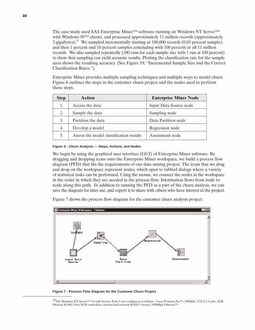
Enterprise Miner provides multiple sampling techniques and multiple ways to model churn.Figure 6 outlines the steps in the customer churn project and the nodes used to performthose steps.

Figure 6 : Churn Analysis — Steps, Actions, and Nodes

We begin by using the graphical user interface (GUI) of Enterprise Miner software. Bydragging and dropping icons onto the Enterprise Miner workspace, we build a process flowdiagram (PFD) that fits the requirements of our data mining project. The icons that we dragand drop on the workspace represent nodes, which open to tabbed dialogs where a varietyof statistical tasks can be performed. Using the mouse, we connect the nodes in the workspacein the order in which they are needed in the process flow. Information flows from node tonode along this path. In addition to running the PFD as a part of the churn analysis, we cansave the diagram for later use, and export it to share with others who have interest in the project.

Figure 7 shows the process flow diagram for the customer churn analysis project.

Figure 7 : Process Flow Diagram for the Customer Churn Project

22

23The Windows NT ServerTM 4.0 with Service Pack 3 was configured as follows: 4-way Pentium ProTM, 200MHz, 512k L2 Cache, 4GBPhysical RAM, Ultra SCSI controllers, internal and external RAID 5 arrays, 100MBps EthernetTM.

Step Action Enterprise Miner Node

1. Access the data Input Data Source node

2. Sample the data Sampling node

3. Partition the data Data Partition node

4. Develop a model Regression node

5. Assess the model classification results Assessment node

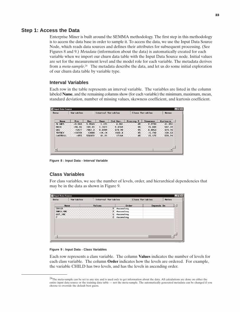
Step 1: Access the DataEnterprise Miner is built around the SEMMA methodology. The first step in this methodologyis to access the data base in order to sample it. To access the data, we use the Input Data SourceNode, which reads data sources and defines their attributes for subsequent processing. (SeeFigures 8 and 9.) Metadata (information about the data) is automatically created for eachvariable when we import our churn data table with the Input Data Source node. Initial valuesare set for the measurement level and the model role for each variable. The metadata derivesfrom a meta-sample.24 The metadata describe the data, and let us do some initial explorationof our churn data table by variable type.

Interval VariablesEach row in the table represents an interval variable. The variables are listed in the columnlabeled Name, and the remaining columns show (for each variable) the minimum, maximum, mean,standard deviation, number of missing values, skewness coefficient, and kurtosis coefficient.

Figure 8 : Input Data - Interval Variable

Class VariablesFor class variables, we see the number of levels, order, and hierarchical dependencies thatmay be in the data as shown in Figure 9.

Figure 9 : Input Data - Class Variables

Each row represents a class variable. The column Values indicates the number of levels foreach class variable. The column Order indicates how the levels are ordered. For example,the variable CHILD has two levels, and has the levels in ascending order.

23

24The meta-sample can be set to any size and is used only to get information about the data. All calculations are done on either theentire input data source or the training data table — not the meta-sample. The automatically generated metadata can be changed if youchoose to override the default best guess.

The variable P represents whether a customer has churned (switched firms). P has two levels:0 indicating churn and 1 indicating no churn. (Enterprise Miner software enables you tomodel either the event or the non-event regardless of whether the event is indicated by 0, 1,or some other means.)

Figure 10 shows the percentage for each level of the variable P. In this case, there is a lowoccurrence of churn (represented by the 0 column). Therefore, we should stratify any subsetsof data we create to ensure that sufficient records are represented. By stratifying, we maintainin the sample the same percentage of records in each level that are present in the entiredatabase. Otherwise, we might obtain a sample with very few or even no customers, whohad switched firms.

Figure 10 : Percentage of Churn and No Churn

For enriched sampling, prior probabilities can be used to weight the data records for properassessment of the prediction results. One weighting scheme is to use the proportion in eachlevel to assign weights to the records in the assessment data table. For example, given avariable with two levels — event and non-event — having the prior probabilities of .04 and.96, respectively, and the proportion of the levels in the assessment data table are .45 and .55,respectively; then the sampling weight for the event level equals .04/.45 and the samplingweight for the non-event level equals .96/.55.

Step 2: Sample the DataAfter accessing the data and performing some initial exploration, we can take a sample. TheSampling node enables us to easily extract a sample from the input data source. For purposesof this case study, samples of different sizes were taken to illustrate that characteristics identifiedin the entire database also are present in the sample. In fact, sample sizes ranging fromoverly large to a small percentage of the data table preserve the characteristics of the entiredatabase. There is no significant loss of information by using small, but representative samples.

24

Percentage

100

70

40

0

0.00 1.00

Legend: 0 indicates churn1 indicates no churn

P

Figure 11 shows the General Dialog page of the Sampling node.

Figure 11 : General Dialog Page

Sampling MethodsAs Figure 11 shows, the Sampling node supports the following types of sampling:

Simple Random By default, every record in the data table has the same probability of being selected forthe sample.

Sampling Every Nth RecordSampling every nth record is also known as systematic sampling.25 This setting computesthe percentage of the population that is required for the sample, or uses the percentagespecified in the General tab. It divides 100 percent by this percentage to come up with anumber. This setting selects all records that are multiples of this number.

Stratified SamplingIn stratified sampling, one or more categorical variables are specified from the input datatable to form strata (or subsets) of the total population. Within each stratum, all recordshave an equal probability of being selected for the sample. Across all strata, however,the records in the input data table generally do not have equal probabilities of beingselected for the sample. We perform stratified sampling to preserve the strata proportionsof the population within the sample. This may improve the classification precision offitted models, which is why we have chosen this method for our case study.

Sampling the First N RecordsThis type of sampling selects the first n records from the input data table for thesample.26 We can specify either a percentage or an absolute number of records to sample in the General tab.

Cluster SamplingThis method builds the sample from a cluster of records that are similar in some way.For example, we want to get all the records of each customer from a random sample ofcustomers.

25

25Sampling every nth record can produce a sample that is not representative of the population, particularly if the input data table is notin random order. If there is a structure to the input data table, then the nth-record sample may reflect only a part of that structure.

26Sampling the first n records can produce a sample that is not representative of the population, particularly if the input data table isnot in random order.

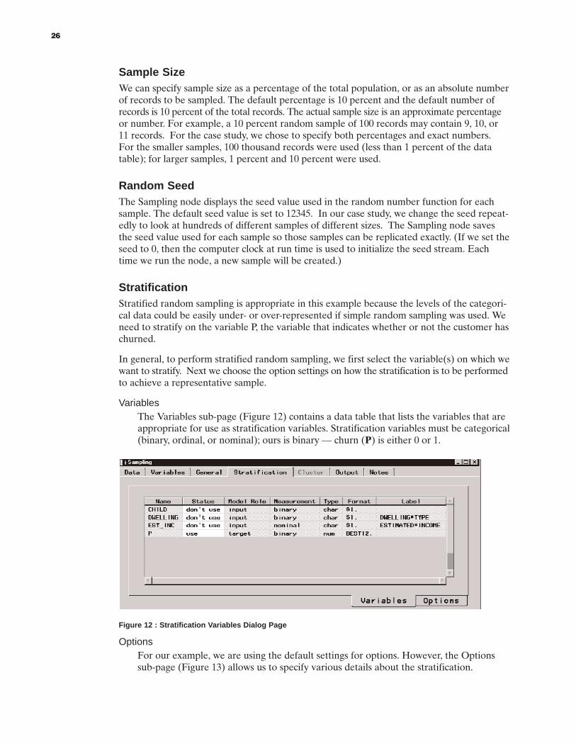
Sample SizeWe can specify sample size as a percentage of the total population, or as an absolute numberof records to be sampled. The default percentage is 10 percent and the default number ofrecords is 10 percent of the total records. The actual sample size is an approximate percentageor number. For example, a 10 percent random sample of 100 records may contain 9, 10, or11 records. For the case study, we chose to specify both percentages and exact numbers.For the smaller samples, 100 thousand records were used (less than 1 percent of the datatable); for larger samples, 1 percent and 10 percent were used.

Random SeedThe Sampling node displays the seed value used in the random number function for eachsample. The default seed value is set to 12345. In our case study, we change the seed repeat-edly to look at hundreds of different samples of different sizes. The Sampling node savesthe seed value used for each sample so those samples can be replicated exactly. (If we set theseed to 0, then the computer clock at run time is used to initialize the seed stream. Eachtime we run the node, a new sample will be created.)

StratificationStratified random sampling is appropriate in this example because the levels of the categori-cal data could be easily under- or over-represented if simple random sampling was used. Weneed to stratify on the variable P, the variable that indicates whether or not the customer haschurned.

In general, to perform stratified random sampling, we first select the variable(s) on which wewant to stratify. Next we choose the option settings on how the stratification is to be performedto achieve a representative sample.

VariablesThe Variables sub-page (Figure 12) contains a data table that lists the variables that areappropriate for use as stratification variables. Stratification variables must be categorical(binary, ordinal, or nominal); ours is binary — churn (P) is either 0 or 1.

Figure 12 : Stratification Variables Dialog Page

OptionsFor our example, we are using the default settings for options. However, the Optionssub-page (Figure 13) allows us to specify various details about the stratification.

26

Figure 13 : Stratification Criteria Dialog Page

The Sampling node supports three criteria for stratified sampling:

• proportional sampling

• equal size27

• optimal allocation28.

All stratified sampling methods in the Sampling node use computations that may requirerounding the number of records within strata. To take a stratified sample on churn, we useproportional stratified sampling, whereby the proportion of records in each stratum is thesame in the sample as it is in the population. We can review the results of the sample inFigure 14, the Sampling Results Browser:

Figure 14 : Sampling Results Browser

27

27The equal size criterion specifies that the Sampling node sample the same number of records from each stratum.

28With optimal allocation, both the proportion of records within strata and the relative standard deviation of a specified variable withinstrata are the same in the sample as in the population.

Step 3: Partition the DataWe use the Data Partition node (Figure 15) to partition the sample data table into three separate, mutually exclusive data tables: training, test, and validation. Note that we also use stratification to create these partitions; we stratify on the variable P. By partitioning thesample, we now can perform split-sample validation, which SAS Institute recommends as a“best practice” in data mining.

The training data table is used for preliminary model fitting. The validation data table isused to monitor and tune the model weights during estimation. The validation data tablealso is used for model assessment. The test data table is an additional holdout data table thatwe can use for further model assessment. In the same way that we used stratified samplingto pull the original sample, we stratify on churn again to partition the data into train, testand validation data tables to ensure sufficient cases of churn in each of them.

Figure 15 : Data Partition Dialog Page

Step 4: Develop a ModelNow that the data have been partitioned into training, test and validation data tables, we canmodel the likelihood of a customer churning. With Enterprise Miner, we could choose amonga number of modeling approaches including various tree-based models as well as variousneural networks. For the purposes of this example, we have chosen a logistic regression model.With the developed model, we learn which variables were important in indicating thelikelihood of customers churning.

The Regression node automatically checks the data, and when a binary target variable isdetected, it uses a logistic regression model. If a continuous target variable is detected, thena linear regression model is used. The Neural Network node and the Decision Tree nodehave similar data checking capabilities.

Figure 16 shows the Regression node Results Browser, which provides part of the estimationresults from fitting the logistic regression model.

28

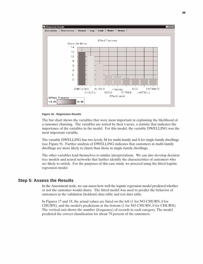
Figure 16 : Regression Results

The bar chart shows the variables that were most important in explaining the likelihood ofa customer churning. The variables are sorted by their t-score, a statistic that indicates theimportance of the variables in the model. For this model, the variable DWELLING was themost important variable.

The variable DWELLING has two levels, M for multi-family and S for single-family dwellings(see Figure 9). Further analysis of DWELLING indicates that customers in multi-familydwellings are more likely to churn than those in single-family dwellings.

The other variables lend themselves to similar interpretations. We can also develop decisiontree models and neural networks that further identify the characteristics of customers whoare likely to switch. For the purposes of this case study, we proceed using the fitted logisticregression model.

Step 5: Assess the ResultsIn the Assessment node, we can assess how well the logistic regression model predicted whetheror not the customer would churn. The fitted model was used to predict the behavior ofcustomers in the validation (holdout) data table and test data table.

In Figures 17 and 18, the actual values are listed on the left (1 for NO CHURN, 0 forCHURN), and the model’s predictions at the bottom (1 for NO CHURN, 0 for CHURN).The vertical axis shows the number (frequency) of records in each category. The modelpredicted the correct classification for about 79 percent of the customers.

29

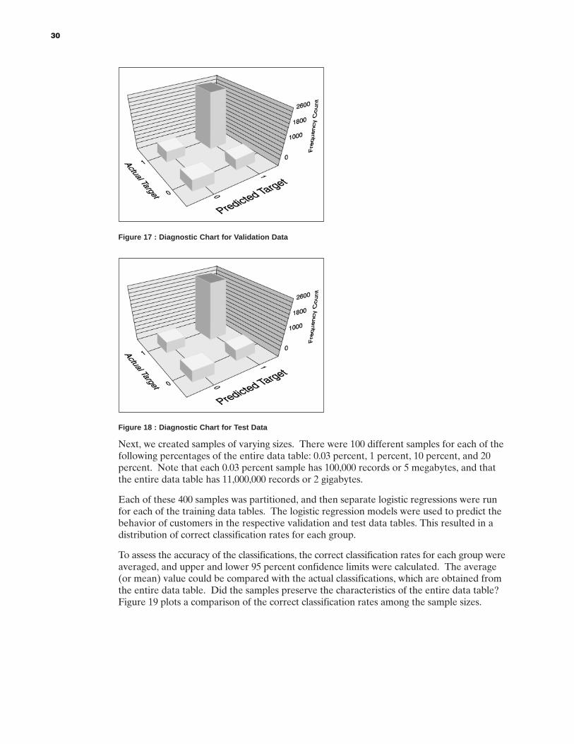
Figure 17 : Diagnostic Chart for Validation Data

Figure 18 : Diagnostic Chart for Test Data

Next, we created samples of varying sizes. There were 100 different samples for each of thefollowing percentages of the entire data table: 0.03 percent, 1 percent, 10 percent, and 20percent. Note that each 0.03 percent sample has 100,000 records or 5 megabytes, and thatthe entire data table has 11,000,000 records or 2 gigabytes.

Each of these 400 samples was partitioned, and then separate logistic regressions were runfor each of the training data tables. The logistic regression models were used to predict thebehavior of customers in the respective validation and test data tables. This resulted in adistribution of correct classification rates for each group.

To assess the accuracy of the classifications, the correct classification rates for each group wereaveraged, and upper and lower 95 percent confidence limits were calculated. The average(or mean) value could be compared with the actual classifications, which are obtained fromthe entire data table. Did the samples preserve the characteristics of the entire data table?Figure 19 plots a comparison of the correct classification rates among the sample sizes.

30

Figure 19 : Incremental Sample Size and the Correct Classification Rates

The mean value of the correct classification rates is shown on the vertical axis. The samplesize is shown on the horizontal axis. The stars plot the mean value of each group, and theplus signs (+) plot the upper and lower 95 percent confidence limits. Note the consistency inthe mean values and in the confidence limits. On average, the different sized-samples providealmost exactly the same accuracy in the classification rates.

In Figure 19, the plot of the correct classification rates looks impressive, but are the resultsreally that good? What about the differences in the classification rates between the samplesizes? To answer these questions, we performed a statistical test on the difference of the means.Figure 20 compares each sample size to the other sample sizes. The first set of three rowsuses the 0.03 percent sample size as the base, and then subtracts the mean of the 1 percent, 10percent, and 20 percent samples. The second set of three rows uses the 1 percent sample asthe base, and so on. The column labeled Difference Between Means shows that the differencein ability to correctly classify is in the fourth decimal place, or in hundredths of a percent.

31

Incremental Sample SizeCorrect Classification Rates

MEAN

0.800

0.795

0.790

+ + + +

✩ ✩ ✩ ✩

+ + + +

0.03% 1% 10% 20%SIZE

Figure 20 : Comparison of Sample Sizes

There are two additional columns in the table that show the 95 percent upper and lowerconfidence limits on the differences between the means. These values are small, and theconfidence limits are “overlapping,” that is, the mean for the 0.03 percent sample size fallswithin the confidence limits for the 20 percent sample.

If a statistically significant difference did exist, then the difference in mean values would beoutside of the confidence interval (upper and lower 95 percent confidence limits). In everycase, the differences are between the confidence limits. We conclude that there are nostatistically significant differences between the mean values of the classification rates. Modelsfit using each group of samples have almost the exact same accuracy in predicting whethercustomers are likely to churn.

Summary of Case Study Results The case study used samples of different sizes to train models, which were used to predictthe behavior of customers. The predicted behavior was compared with the actual behaviorto calculate classification rates. The classification rates had essentially the same level ofaccuracy for models trained using samples having 0.03 percent, 1 percent, 10 percent, and 20percent of the data. These results confirm that properly performed sampling can maintainprecision. Moreover, sampling saves processing time and enables you to validate and testthe results.

32

Simultaneous SimultaneousLower Difference Upper

Sample Size Confidence Between ConfidenceComparison Limit Means Limit

0.03%-1% -0.0008941 -0.00039 0.000110.03%-10% -0.0007792 -0.00028 0.0002250.03%-20% -0.0016483 -0.00016 0.001337

1% -0.03% -0.0001102 0.00392 0.0008941% -10% -0.0003872 0.000115 0.0006171% -20% -0.0012563 0.000236 0.001729

10% -0.03% -0.0002252 0.000277 0.00077910% -1% -0.0006171 -0.00011 0.00038710% -20% -0.0013713 0.000121 0.001614

20% -0.03% -0.0013367 0.000156 0.00164820% -1% -0.0017286 -0.00024 0.00125620% -10% -0.0016136 -0.00012 0.001371

SAS Institute: A Leader in Data Mining Solutions

For more than 20 years, SAS Institute Inc. has distinguished itself by providing world-classtechnology and the technical know-how to solve customers’ business problems around the globe.

For data mining, the Institute has developed SAS Enterprise Miner™ software, whichenables business leaders to make better business decisions by controlling the process thatmoves from data, to information, to business intelligence. However, moving from data tobusiness intelligence requires taking logical steps that will ensure the results of your datamining efforts are reliable, cost efficient, and timely.

In data mining, reliability means the results are based on modern analytical practices. Thus,inferences you make are quantifiable; that is, you can say with a specific degree of confidence —for example a 95 percent confidence level — that the output of your data mining project isbetween the values x and y.

Cost efficiency refers to the balance between, on the one hand, the reliability of the resultsand, on the other hand, the human and computing resources that are expended obtainingthe results.

Timeliness refers to the need to obtain reliable, cost-effective results when you need them;that is, in time to act proactively in a fast-moving, highly competitive global economy.

33

References

American Statistical Association, Blue Ribbon Panel on the Census, (1996 September). Report of the President’s Blue Rib-bon Panel on the Census. Retrieved September 8, 1998 from the World Wide Web: http://www.amstat.org/census.html

Breslow, N.E. and W. Day, (1980), Statistical Methods in Cancer Research. Volume 1 - The Analysis of Case-Control Studies,Lyon: IARC Scientific Publication No. 32.

Cochran, William G., (1977), Sampling Techniques, New York: John Wiley & Sons, Inc.

Elder, John F., IV and Daryl Pregibon, (1996), Advances in Knowledge Discovery & Data Mining, “A Statistical Perspectiveon KDD.”

Gladstone, Brooke, (1998), “Error Naming Campaign Winner,” NPR Online, Morning Edition, November 3, 1998,Retrieved November 6, 1998 from the World Wide Web:http://www.npr.org/programs/morning/archives/1998/981103.me.html

Greenhouse, Linda, (1998), “High Court to Hear Appeal of Census Ruling,” The New York Times on the Web, (September 11),Retrieved via site search on “census” September 11, 1998 from the World Wide Web: http://www.nytimes.com

Gribbon, John, (1996), Companion to the Cosmos, New York: Little, Brown and Company.

Hays, William L., (1981), Statistics, New York: CBS College Publishing.

International Data Corporation, (1998 June), “Information Access Tools: 1998 Worldwide Markets And Trends,” IDC#15932, Volume: 1.

Manski, C. F. and Daniel McFadden, (1981), Structural Analysis of discrete data with Applications, Cambridge, Mass: MIT Press.

McCullough, David, (1992), Truman, New York: Simon & Schuster.

META Group, (1997 August 19), “Data Mining the SAS Data Warehouse,” Application Delivery Strategies, File #594.

Phillips, John L., (1996), How to Think About Statistics, Fifth Edition, New York: W.H. Freeman and Company.

Potts, William J. E., (1997), Data Mining Using SAS Enterprise Miner Software. Cary, North Carolina: SAS Institute Inc.

Ripley, B.D., (1996), Pattern Recognition and Neural Networks, Cambridge: Cambridge University Press.

Ross, Sheldon, (1998), A First Course in Probability, Fifth Edition, Upper Saddle River, New Jersey: Prentice-Hall, Inc.

Saerndal, Carl-Erik, Bengt Swensson, and Jan Wretman, (1992), Model Assisted Survey Sampling. New York: Springer-Verlag.

Sarle, W.S., ed. (1997), Neural Network FAQ, periodic posting to the Usenet newsgroup comp.ai.neural-nets, URL:ftp://ftp.sas.com/pub/neural/FAQ.html

Snedecor, George W. and William G. Cochran, (1989), Statistical Methods, Eighth Edition, Ames, Iowa: The Iowa State University Press.

U.S Bureau of the Census, (1992), Statistical Abstract of the United States, 112th edition, Washington, DC.

U.S. House of Representatives v. U.S. Department of Commerce, et al, (1998), Civil Action No. 98-0456 (Three JudgeCourt) (RCL, DHG, RMU), Opinion filed August 24, 1998 by Circuit Judge Douglas H. Ginsburg, and District CourtJudges Royce C. Lamberth and Ricardo M. Urbina.

Westphal, Christopher and Teresa Blaxton, (1998), Data Mining Solutions: Methods and Tools for Solving Real-World Problems, John Wiley and Sons.

34

Recommended Reading

Data MiningBerry, Michael J. A. and Gordon Linoff, (1997), Data Mining Techniques, New York: John Wiley & Sons, Inc.

SAS Institute Inc., (1997), SAS Institute White Paper, Business Intelligence Systems and Data Mining, Cary, NC: SAS Institute Inc.

SAS Institute Inc., (1998), SAS Institute White Paper, Finding the Solution to Data Mining: A Map of the Features andComponents of SAS Enterprise Miner™ Software, Cary, NC: SAS Institute Inc.

SAS Institute Inc., (1998), SAS Institute White Paper, From Data to Business Advantage: Data Mining, The SEMMAMethodology and the SAS® System, Cary, NC: SAS Institute Inc.

Weiss, Sholom M. and Nitin Indurkhya, (1998), Predictive Data Mining: A Practical Guide, San Francisco, California:Morgan Kaufmann Publishers, Inc.

Data WarehousingInmon, W. H., (1993), Building the Data Warehouse, New York: John Wiley & Sons, Inc.

SAS Institute Inc., (1995), SAS Institute White Paper, Building a SAS Data Warehouse, Cary, NC: SAS Institute Inc.

SAS Institute Inc., (1998), SAS Institute White Paper, SAS Institute’s Rapid Warehousing Methodology, Cary, NC: SAS Institute Inc.

Singh, Harry, (1998), Data Warehousing Concepts, Technologies, Implementations, and Management, Upper SaddleRiver, New Jersey: Prentice-Hall, Inc.

Statistics Hays, William L. (1981), Statistics. New York: Holt, Rinehart and Winston.

Hildebrand, David K. and R. Lyman Ott, (1996), Basic Statistical Ideas for Managers, New York: Duxbury Press.

Mendenhall, William and Richard L. Scheaffer, (1973), Mathematical Statistics with Applications. North Scituate,Massachusetts.

Phillips, John L., (1996), How to Think About Statistics, Fifth Edition, New York: W.H. Freeman and Company.

35

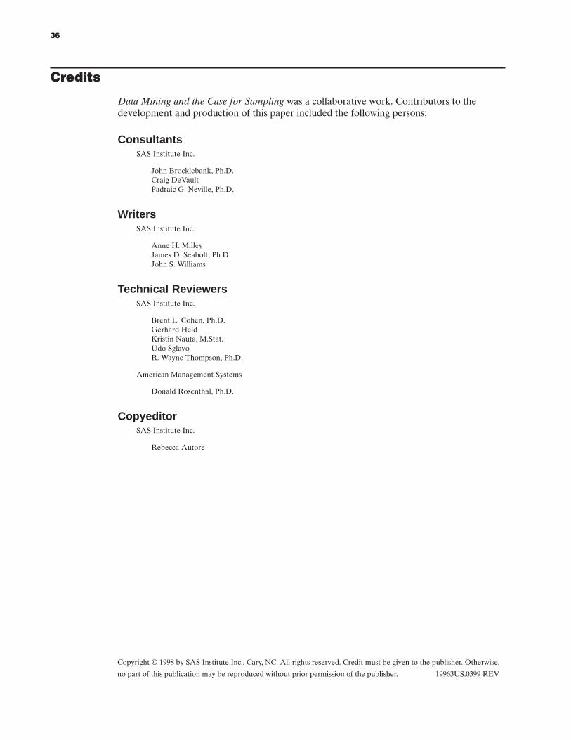
Credits

Data Mining and the Case for Sampling was a collaborative work. Contributors to the development and production of this paper included the following persons:

ConsultantsSAS Institute Inc.

John Brocklebank, Ph.D.Craig DeVaultPadraic G. Neville, Ph.D.

WritersSAS Institute Inc.

Anne H. MilleyJames D. Seabolt, Ph.D. John S. Williams

Technical ReviewersSAS Institute Inc.

Brent L. Cohen, Ph.D.Gerhard HeldKristin Nauta, M.Stat.Udo SglavoR. Wayne Thompson, Ph.D.

American Management Systems

Donald Rosenthal, Ph.D.

CopyeditorSAS Institute Inc.

Rebecca Autore

36

Copyright © 1998 by SAS Institute Inc., Cary, NC. All rights reserved. Credit must be given to the publisher. Otherwise,

no part of this publication may be reproduced without prior permission of the publisher. 19963US.0399 REV