data mining and analysis on twitter -...
TRANSCRIPT

1
Semester Project ReportSemester Project ReportSemester Project ReportSemester Project Report
Data Mining and Analysis on TwitterData Mining and Analysis on TwitterData Mining and Analysis on TwitterData Mining and Analysis on Twitter
Pulkit Goyal ([email protected])
Sapan Diwakar ([email protected])
January 14, 2011
ProfessorProfessorProfessorProfessor::::
Prof. Pascal Frossard
SupervisorSupervisorSupervisorSupervisor::::
Xiaowen Dong

2
Page intentionally left blank

3
Table Table Table Table of Contentsof Contentsof Contentsof Contents Abstract ................................................................................................................................ 5
1 Introduction ................................................................................................................... 5
1.1. Social Media ............................................................................................................ 5
1.2. Twitter .................................................................................................................... 6
1.3. Communities in Social Networks ............................................................................. 7
1.4. Organisation of the report ....................................................................................... 8
2 System Design and Data Collection ................................................................................ 8
2.1. System Architecture ................................................................................................ 8
2.2. Technologies Used .................................................................................................. 10
2.3. Data Collection ...................................................................................................... 11
2.3.1 Geo-tagged tweets ........................................................................................... 12
2.3.2 Tweets about a topic ....................................................................................... 12
2.3.3 Tweets from a group of users .......................................................................... 13
3 Visualizations ................................................................................................................ 15
3.1. Visualization of tweets collected by location .......................................................... 15
3.2. Visualizations for tweets collected by keywords ...................................................... 17
4 Community Detection ................................................................................................... 18
4.1. Background ............................................................................................................ 18
4.1.1 Hierarchical Clustering: ................................................................................... 19
4.1.2 Spectral clustering: .......................................................................................... 20
4.1.3 Similarity Measures between users .................................................................. 21
4.2. Results and analysis on small dataset..................................................................... 23
4.3. Results and analysis on large dataset ..................................................................... 27
5 Future mentions between users ..................................................................................... 33
6 Conclusion & Future Work ........................................................................................... 36
7 References ..................................................................................................................... 37

4
Page intentionally left blank
5
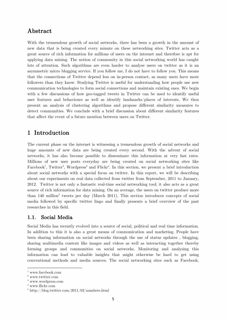
AbstractAbstractAbstractAbstract
With the tremendous growth of social networks, there has been a growth in the amount of
new data that is being created every minute on these networking sites. Twitter acts as a
great source of rich information for millions of users on the internet and therefore is apt for
applying data mining. The notion of community in this social networking world has caught
lots of attention. Such algorithms are even harder to analyse users on twitter as it is an
asymmetric micro blogging service. If you follow me, I do not have to follow you. This means
that the connections of Twitter depend less on in-person contact, as many users have more
followers than they know. Studying Twitter is useful for understanding how people use new
communication technologies to form social connections and maintain existing ones. We begin
with a few discussions of how geo-tagged tweets in Twitter can be used to identify useful
user features and behaviours as well as identify landmarks/places of interests. We then
present an analysis of clustering algorithms and propose different similarity measures to
detect communities. We conclude with a brief discussion about different similarity features
that affect the event of a future mention between users on Twitter.
1111 IntroductionIntroductionIntroductionIntroduction
The current phase on the internet is witnessing a tremendous growth of social networks and
huge amounts of new data are being created every second. With the advent of social
networks, it has also become possible to disseminate this information at very fast rates.
Millions of new user posts everyday are being created on social networking sites like
Facebook1, Twitter2, Wordpress3 and Flickr4. In this section, we present a brief introduction
about social networks with a special focus on twitter. In this report, we will be describing
about our experiments on real data collected from twitter from September, 2011 to January,
2012. Twitter is not only a fantastic real-time social networking tool; it also acts as a great
source of rich information for data mining. On an average, the users on twitter produce more
than 140 million5 tweets per day (March 2011). This section introduces concepts of social
media followed by specific twitter lingo and finally presents a brief overview of the past
researches in this field.
1.1.1.1.1.1.1.1. Social MediaSocial MediaSocial MediaSocial Media
Social Media has recently evolved into a source of social, political and real time information.
In addition to this it is also a great means of communication and marketing. People have
been sharing information on social networks through the use of status updates , blogging,
sharing multimedia content like images and videos as well as interacting together thereby
forming groups and communities on social networks. Monitoring and analysing this
information can lead to valuable insights that might otherwise be hard to get using
conventional methods and media sources. The social networking sites such as Facebook,
1 www.facebook.com 2 www.twitter.com 3 www.wordpress.com 4 www.flickr.com 5 http://blog.twitter.com/2011/03/numbers.html

6
Twitter and Flickr provide a new way to share the information among them and get frequent
updates. In addition to this, the sites also allow sharing of additional information which can
be important in analysing the contents, e.g. location etc.
The social media has an advantage over conventional media sources as it is managed by the
users. Conventional media only allowed users to gain information that was provided to them.
The flow of information was only one-sided from the media to user. With social networks,
however, the users now have the ability to respond to the news and events around them and
provide their opinion on them as well as share them. This leads to the evolution of a multi-
way mode of information dissemination in which the users post information along with other
information like links, images and videos. As a result, a user generated model of information
is generated. The social graph of users and their connections on the social networks plays an
important role in analysing this information model in order to obtain meaningful data from
the vast amount of “user generated content” that is created every day.
Since, the micro-blogging6 sites like Facebook, Twitter and Flickr allow users to share short
messages and multimedia, they have become an instant source of information through which
users from all around the world can remain connected and get to know about the
information from several sources.
1.2.1.2.1.2.1.2. TwTwTwTwitteritteritteritter
Twitter launched as a micro-blogging website in March 2006 which allows users to post
status updates of up to 140 characters, also known popularly as tweets. Since its launch,
twitter has amassed a large user base and now has over 300 million users (June, 2011) [1].
Twitter allows its users to post short status messages called tweets. Tweets can be posted
(tweeted) from various sources which include the twitter website, twitter mobile applications
as well as several third party applications/websites (after authentication). Users also have
the control over the privacy features and they can choose to either make their tweets public
which make the tweets visible to any one or make them private which restricts the access to
only some users who obtain permission from the user. Users can follow other users on twitter
which gives them access to their tweets on their homepage on twitter.
Twitter allows several other features. It allows users to reply to tweets of other users by
clicking on the reply button on the tweet of the user who one wants to reply to. This is a
way to say something back in response to a user’s tweet. In addition to this, users can also
mention other users in their tweets by adding ‘@’ to the username of another user in a tweet.
A mention is a way to refer to some other user. Another popular concept of twitter is
retweeting. A retweet is an event of sharing someone else’s tweet to our followers. Retweet
plays an important part in the dissemination of information on twitter. Users can also add a
hashtag in their tweets by adding a ‘#’ sign before relevant keywords. This is used to
categorize those tweets to show more easily in twitter search. Very popular hash tags on
twitter become trending topics on twitter.
An important feature of twitter that separates it from other social networking sites like
Facebook is that the relationship of following and being followed are not necessarily two
6 Websites that allow a blog that contains very small elements

7
ways. Following someone is equivalent to subscribing to a blog; the follower gets all the
status updates of the user that he follows.
An important characteristic that emerges from the network of twitter users is the Social
Graph. A social graph is a graph derived from the connections between the users. These
connections can be of many forms. The most straightforward social graph that can be
created from twitter is a graph that contains following and being followed relationship
among users. There have been several researches [2] [3] [4] focused towards studying these
social graphs and finding some features from such graphs. There are a few properties
common to many social graphs: the small-world property, power law degree distributions and
network transitivity (two users who have a common neighbour are more likely to be
connected together rather than with some other user who with whom they don’t share a
neighbour).
The social graphs generally also contain a clustered structure meaning that certain users
form a tightly knit group with very low connectivity between different such groups. These
clusters may also contain other similarity features like similar tweets or locations etc. A
community in a social graph can be described as a group of vertices that have more edges
between them than any other vertex that belongs to other group in the social graph.
1.3.1.3.1.3.1.3. Communities in Social NetworksCommunities in Social NetworksCommunities in Social NetworksCommunities in Social Networks
The topology of complex social networks has been studied extensively in the past. It has
been found that social networks exhibit a very clear community structure [5] [6]. This
community structure can occur due to personal as well as political or cultural reasons. The
analysis of community structure on social networks can be used to figure out influential
tweets and user groups for specific brands, sports, political organizations and technologies.
The communities have also been analysed to discover disaster events (e.g. in [7]) etc.
Figure Figure Figure Figure 1111: : : : The Karate Club network
Figure 1 presents an example of a traditional network, Zachary’s karate club network [8]
which has been widely used to evaluate community structure and detection in networks. The

8
network shows social interactions between individuals at a karate club at an American
University. The club split into two groups as a result of a dispute between club’s
administrator and principal karate teacher. The real social structure in the graph is shown
by squares and circles depicting the group of individuals who sided with the administrator
and others with the karate teacher. However, there have been several researches and
community detection methods have also come up with another meaningful clustering result
as shown by different colours in the graph.
Majority of the algorithms for social network analysis only consider the social connections
between users for the analysis of clusters between users and ignore the vast amount of other
information available in the current social networks. In addition to social connections,
twitter can be used to obtain different types of links among users like mentions, similarity
between tweets of different users, retweets, hashtags and locations.
We analyse several different clustering algorithms by using different link structure between
users by taking into account the social connections, mentions, hash tag similarity, tweet
similarity etc. among users. We also analyse two different types of algorithms, firstly where
we know the ground truth data and therefore the number of clusters, and then, the
algorithms that allow clustering without using the information about number of clusters.
1.4.1.4.1.4.1.4. Organisation of the reportOrganisation of the reportOrganisation of the reportOrganisation of the report
The further sections of the report are organised as follows. We begin by presenting an
overview of our data collection system that includes the environment that we use for
collecting data. In addition to this, we also describe more about the filters using which we
collect our data in section 2. In section 3 we present a top level analysis of different types of
collected data and present visualizations. We then present an analysis of clustering
algorithms on twitter and introduce several different types of similarity measures in order to
improve clustering results in section 4. Finally, we present a brief analysis of reasons for
future mentions in twitter in section 5.
2222 System Design and System Design and System Design and System Design and Data CollectionData CollectionData CollectionData Collection
In this section we present a brief overview of the design of our system for data collection and
the experimental setup and filters based on which we collect our data. We follow this brief
description by the goals of the data collection system.
2.1.2.1.2.1.2.1. System Architecture System Architecture System Architecture System Architecture
Figure 2 describes the scope of the system that we built along with the entities outside the
system that it interacts with and a description of the interfaces between these entities.
Although the early web was about human-machine interaction, today's web is about
machine-machine interaction, enabled using web services. These services exist for most
popular websites—from various Google services to LinkedIn, Facebook, and Twitter. Web
services create APIs through which external applications can query or manipulate content on
websites. Twitter API7 provides interfaces to query Twitter for data based on certain filters.
7 https://dev.twitter.com

9
Each API represents a facet of Twitter, and allows developers to build upon and extend their
applications in new and creative ways. Twitter provides three kinds of APIs:
• SearchSearchSearchSearch APIAPIAPIAPI
The Search API allows users to query for Twitter content. This includes finding
tweets for a set of keywords, users or location posted in the past.
• RESTRESTRESTREST APIAPIAPIAPI
The REST API enables developers to access some of the core primitives of
Twitter including timelines, status updates, and user information. In addition to
offering programmatic access to the timeline, status, and user objects, this API
also enables developers a multitude of integration opportunities to interact with
Twitter.
• StreamingStreamingStreamingStreaming APIAPIAPIAPI
The Streaming API allows for large quantities of keywords to be specified and
tracked, retrieving geo-tagged tweets from a certain region, or have the public
statuses of a user set returned. It allows users to establish and maintain a long-
lived HTTP connection with the Twitter server.
Figure Figure Figure Figure 2222: : : : System Architecture
We now present in Figure 3 the schema of our database that represents the information that
we collect for the users and tweets. The user table contains the information for the users on
twitter. We contain all the available profile information from twitter for the users. This
enables us to utilize different kinds of information other than just the social connections for
the clustering algorithms. The status table contains various information related to tweet
posted by user. The text attribute contain the actual text posted by a given user. In addition
to this it also contains the longitude and latitude of the location from where tweet has been
posted, time etc. It also contains a link to the user table which points to the user who has
posted a particular tweet. We also store the information about the place from which the
tweet was posted in the place table. This allows us to collect all tweets that have been
collected from the same place easily. The tweets can also contain several hash tags,
mentions, links, and images which are stored in the respective tables in the database. We
store these information separately in different tables so that we don’t have to perform text
manipulation to obtain these information from the database.

10
Figure Figure Figure Figure 3333: : : : Database Schema for Data collection
2.2.2.2.2.2.2.2. TechnologiesTechnologiesTechnologiesTechnologies UsedUsedUsedUsed
In this section we present a brief overview about the technologies used for building the
system for collecting data as well as preparing further analysis.
• Eclipse8: We use Eclipse for the development. The reason for selecting Eclipse is its
wide community. Most of the plugins can be easily integrated with it.
• Maven9: Apache Maven is a software project management and comprehension tool.
Based on the concept of a project object model, Maven can manage a project's build,
reporting and documentation from a central piece of information. Maven uses a
construct known as a Project Object Model to describe the software project being
8 Eclipse is an integrated development environment (IDE), www.eclipse.org 9 www.maven.apache.org

11
built, its dependencies on other external modules and components, and the build
order. It comes with pre-defined targets for performing certain well defined tasks such
as compilation of code and its packaging.
• Hibernate10: Hibernate's primary feature is mapping from Java classes to database
tables (and from Java data types to SQL data types). Hibernate also provides data
query and retrieval facilities. Hibernate generates the SQL calls and attempts to
relieve the developer from manual result set handling and object conversion and keep
the application portable to all supported SQL databases with little performance
overhead.
Hibernate is basically an ORM Framework which allows you to perform database
activities without bothering about the Database change. With respect to
performance, hibernate provide the capability to reduce the number of database trips
by creating the batch processing and session cache and second level cache. It also
supports the transactions. More than this all, it is very easy to make a cleaner
separation of Data Access Layer from Business logic layer.
With all the capabilities mention above it is fast and easy to learn hibernate, develop
application and maintain easily. The core drawback of JDBC is that it doesn’t allow
you to store object directly to the database you must convert the objects to a
relational format.
• Twitter4J11: It is an open-source, mavenized and Google App Engine safe Java library
for Twitter API which is released under BSD license. It allows to easily integrate a
Java application with the twitter service. We have used it to collect tweets using its
streaming and search methods implementation from the twitter4j package.
• Git12 and Github13: Git is a distributed revision control system. Every Git working
directory is a full-fledged repository with complete history and full revision tracking
capabilities, not dependent on network access or a central server. GitHub is a web-
based hosting service for software development projects that use the Git revision
control system. GitHub offers both commercial plans and free accounts for open
source projects. We use git for version control and github to manage code between
different systems and developers.
• Matlab14: We use Matlab for the implementation of various clustering algorithms as
it provides several tools for the analysis of matrices in which the social connection
graphs can be represented easily.
2.3.2.3.2.3.2.3. Data CollectionData CollectionData CollectionData Collection
We collect different type of data in order to fulfil different goals. In this section, we provide
a brief description of the data that we collect using our system followed by the objectives
that the collected data helps to achieve. We collect data of the following three types:
10 www.hibernate.org 11 www.twitter4j.org 12 http://git-scm.com/ 13 https://github.com/ 14 www.mathworks.com/

12
2.3.12.3.12.3.12.3.1 GeoGeoGeoGeo----tagged tweetstagged tweetstagged tweetstagged tweets
Twitter's Tweet with Your Location feature allows users to selectively add location
information to their Tweets. The users who choose to add location to their tweets will be
able to add their location information to new tweets that they post. Some applications allow
users to tweet with their exact geo-location coordinates of the location from which they
tweet. Figure 4 shows an example of a geo-tagged tweet posted on twitter.
We collect tweets that come from the following five cities:
• London: (51.3695, -0.3475)15 to (51.6435, 0.0915)
• New York: (40.633¸-74.11) to ( 40.800, -73.89)
• Paris: (48.784, 2.241) to (48.929, 2.2460666)
• San Francisco: (37.6925, -122.529) to (37.8661, -122.3094)
• Mumbai: (18.875, 72.55) to (19.275, 73.15)
Figure Figure Figure Figure 4444: : : : An example of geo-tagged tweet
The tweets from these cities can be used to achieve the following objectives.
• Model the spread of interests around the world. The data containing geo location
coordinates can be used to find out the content similarity between the tweets around
different cities in the world to discover the keywords that are popular throughout the
world. This information can also be used to target special interest groups in different
cities using different campaigns. There have been several researches in this field of
social information modelling based on locations. The authors in [9] outline
navigational and social aspects of such location based systems. Such an analysis can
be used to analyse the timed information of different events, locations of different
keywords as well as the rate of information flow.
• Predict future/current events. The tweets’ data collected from different cities has
been used to predict future and current events as well as the result of elections [10],
popularity of movies etc. [11] as well as prediction of disaster events [7].
2.3.22.3.22.3.22.3.2 Tweets about a topicTweets about a topicTweets about a topicTweets about a topic
The next set of tweets that we collect are based on a set of keywords that describe a topic in
real world. We collect tweets that contain the following two sets of keywords:
15 (latitude, longitude) pairs representing the starting and ending point of the bounding box

13
• Tweets about Apple Inc.Tweets about Apple Inc.Tweets about Apple Inc.Tweets about Apple Inc.16: apple, mac, macbook, macbookair, macbookpro, os x,
osx, osxlion, ipod, ipodshuffle, ipodnano, ipodclassic, ipodtouch, itunes, iphone,
iphone3, iphone3s, iphone4, iphone4s, iphone5, ios, ios4, ios5, ipad, ipad2, ipad3
Figure Figure Figure Figure 5555: : : : An example tweet about Apple Inc.
• Tweets about Manchester UnitedTweets about Manchester UnitedTweets about Manchester UnitedTweets about Manchester United17: manchesterunited, manchester united,
manchester utd, man united, manutd, man utd, manu, mufc
Figure Figure Figure Figure 6666: : : : An example tweet about Manchester United
These set of tweets allow us to achieve different goals. These set of tweets again serve
the goal of modelling the spread of user interests around the world as well as the
popularity of these topics at different points in time. This can again be used to model the
rate of information flow on the internet. The collection of tweets from these keywords
can also help these organisations to target different user groups in different places as well
as try to obtain product reviews and popularity of soccer matches. This type of modelling
has been done in the past with the goal of marketing for different companies [12].
2.3.32.3.32.3.32.3.3 Tweets from a group of usersTweets from a group of usersTweets from a group of usersTweets from a group of users
Finally, we also collect tweets from a group of users on twitter. We collected this group of
users by looking at the friends and followers of a central user18. We first collected the users
that follow the central user and the users that are being followed by him. That is we collect
users that have any of the two kinds of links with the central users. We then do the same for
the users collected in the previous step. This means that we collect the followers and friends
of a central user up to two hops in the social connection hierarchy. Our aim with the
collection of these users is to analyse the meaningful connections between these groups of
users and therefore, we excluded celebrities or other very popular users (users which have
more than 1000 followers or follows more than 5000 other users) from our study as these
would have many relationships outside a tightly connected community of users.
Figure 7 presents an overview of the collection system. The links show a directed relationship
between users. A link from user ‘a’ to user ‘b’ means that ‘a’ follows ‘b’ on twitter. The
being followed relation has not been shown in the figure as it is just the reverse of the
16 Multinational corporation that designs and markets consumer electronics, computer software, and personal computers 17 English professional football club, based in Old Trafford, Greater Manchester, that plays in the Premier League 18 Username: ‘_aakash’

14
following relationship between users. The blue links are the links that we follow to collect the
users. The node with dark blue colour in the centre represents the central user that we use
as a starting point for our collection system. The red links are the links at which we stop
collecting the users further. This allows us to limit our system to a limited number of users
as compared to the large user base of twitter.
Figure Figure Figure Figure 7777: : : : Overview of links we use to collect users
We collect all the public profile information of the users that belong to these groups. In
addition to this, we also collect the tweets that these users post. The collection of this
information allows us to model different types of social link and relationships between these
users. Further in the report we will also present a detailed analysis of the social information
that we obtain and how we use this information to detect the community structure in this
group of users. The collection of this information allows us to achieve the following goals.
• Model relationships among users. As explained before, we can use the social
connections between these users to model their relationships on twitter and also
detect a community structure that corresponds to a tight cluster of these users on
twitter.

15
• In addition to this, we can also model the common interest of these users using the
content of their tweets. We also use several other meta-data contained in the tweets
to cluster the users.
3333 VisualizationsVisualizationsVisualizationsVisualizations
We now present a few visualizations and analysis on the data collected using the locations
and keywords that allow us to draw certain simple inferences from the above tweet data.
3.1.3.1.3.1.3.1. Visualization of tweets collected by locationVisualization of tweets collected by locationVisualization of tweets collected by locationVisualization of tweets collected by location
We begin by presenting a very simple analysis of how the geo-tagged tweets from a city can
be used to identify some places of interest in the city. Without any loss of generality, let us
present an example of visualizing tweets in London. These are the geo-tagged tweets
collected for one week (16 Aug, 2011 to 22 Aug, 2011) from London as per the bounding box
coordinates given earlier (in Section 2.3.1). We plot these tweets as small blue points on a
map of London using Geo-Commons19.
Figure Figure Figure Figure 8888: : : : Tweets in London for one week with two places with high density of tweets marked in red
The Figure 8 shows the visualization for the data collected as per the above setup. We can
see from the visualization that there is particularly large density of tweets from a few places.
We have identified and marked two of such places on the map. This presents an example of
how the tweets and their density in a particular location can be used to identify places of
interest and important landmarks at that place.
19 www.geocommons.com

16
In addition to the detection of landmarks in cities, we also show through the above example
another kind of analysis using the tweet density. The high density of tweets at the Oval
cricket ground is as a result of the India vs England cricket match20 during the week from 18
Aug, 2011 to 22 Aug, 2011 as a result of which there is a high density of tweets from the
cricket ground. Hence, one can also discover events that are going on by looking at the data
from the tweets as well as the density of tweets at certain places.
Another important information that we can infer from the above visualization of tweets in
London is that most of the tweets align with the roads/streets rather than from open
grounds.
The next visualization that we present can help us to study the user behaviours at different
times. It can give us a clue to where most of the user tweets come from during different
times in a day. This information can be used by organisers to plan their events so that they
can attract a maximum amount of crowd. The setup for the following experiment consists of
tweets collected from London on 18 Aug, 2011 from 00:00h to 23:59h and then aggregated
into Greater London Ward Boundaries21 dataset using Geo-Commons. The map shown in
Figure 9 below represents the one of the figures obtained by using the experimental setup for
tweets from 18h to 21h.
Figure Figure Figure Figure 9999: : : : Tweets in London from 18h to 21h on 18 Aug, 2011 aggregated by Greater London Wards
20 www.espncricinfo.com/ci/engine/current/match/474475.html 21 http://geocommons.com/overlays/142833

17
We have also tried to plot the geo-tagged tweets on a map based on their time information.
By looking at the location of tweets at different points in time over a week, we can observe
that the location and density of tweets remains periodic over time and we can see the
evolution of tweets as the day progresses. We can also make some simple inferences by using
the tweet’s location and time information. E.g. By looking at the information, we can say
that there are no tweets from the river during the night as opposed to high density of tweets
from the river during day times. Similarly, the number of tweets in the evening is much
more than as compared to day time or after midnight.
3.2.3.2.3.2.3.2. Visualizations for tweets collected by keywordsVisualizations for tweets collected by keywordsVisualizations for tweets collected by keywordsVisualizations for tweets collected by keywords
Now, we present some visualizations obtained by plotting the geo-tagged tweets that have
been collected using the keywords based on two topics as described in Section 2.3.2. After
presenting the visualization results, we also try to extract certain inferences from the two
visualizations. The following visualizations contain geo-tagged tweets that contain the
keywords mentioned above from 27 October, 2011 to 8 Nov, 2011.
Figure 10 contains the tweets for the topic ‘Manchester United’ in the specified time frame.
By looking at the visualization results, we can infer that most of the tweets mentioning
Manchester United come from in and around Europe. This can be because of the fact that
Manchester United plays in the English Premiere League and has its home ground in
Manchester. In addition to this, we also find that there are a lot of tweets from countries
whose players play for Manchester United. We also present a few such examples in the
visualization where we show a tweet mentioning the player ‘Nani’ coming from Portugal and
another tweet mentioning the player ‘Anderson’ from Brazil. In addition to these inferences,
we also find that there are a lot of tweets from Indonesia and Malaysia that talk about
Manchester United. This is because of the fact that Manchester United has invested a lot in
these countries and is therefore very popular.
Figure Figure Figure Figure 10101010: : : : Tweets about the topic 'Manchester United'
Figure 11 on the other hand shows the geo-tagged tweets about the topic ‘Apple Inc.’. We
find that as opposed to tweets about Manchester United which were mostly from Europe,
Apple has a much larger popularity and tweets about Apple come mostly from North

18
America and Europe. This can be explained as the popularity and usage of products of Apple
in these regions.
When we compare the results of Apple and Manchester United, we can see that Apple is
more popular than Manchester United as the volume of tweets for Apple is much larger than
Manchester United. E.g. For the above setup of two weeks, we obtained more than 32,000
geo-tagged tweets for Apple as opposed to only 1,400 geo-tagged tweets for Manchester
United. Another inference that we can draw from the above visualizations is that interests
about Apple are spread over the world whereas for Manchester United, the interests are
restricted mostly to Europe and few countries in Asia.
Figure Figure Figure Figure 11111111: : : : Tweets about the topic 'Apple'
4444 Community DetectionCommunity DetectionCommunity DetectionCommunity Detection
4.1.4.1.4.1.4.1. BackgroundBackgroundBackgroundBackground
Community detection/clustering is the process of taking collections of objects such as tweets,
location similarity and organising them into groups based on their similarity. The
organisation into groups should be such that similar objects belong to the same cluster
whereas there is little or no similarity between objects that belong to different clusters. The
main elements of the problem themselves, i. e. the concepts of community and partition, are
not rigorously defined, and require some degree of arbitrariness and/or common sense. It is
important to stress that the identification of structural clusters is possible only if graphs are
sparse22, i. e. if the number of edges m is of the order of the number of nodes n of the graph.
If m >> n, the distribution of edges among the nodes is too homogeneous for communities to
make sense.
22 This is generally true only for unweighted graphs. There have been clustering algorithms that perform considerably well on graphs with large number of weighted edges with heterogeneous edge weights.

19
Before looking into the clustering algorithms for graphs, let us first discuss about the notion
of communities in social networks. There is not one globally accepted definition for
communities in social networks. But, from intuition, one can say that the communities
should have an important property that the nodes inside a community should have more
connections among them rather than between nodes from different communities.
Communities are the parts of graph with few ties with the rest of the system.
There have been several researches in the field of clustering in the past. The clustering
algorithms can be grouped into two major classes:
4.1.14.1.14.1.14.1.1 Hierarchical Clustering: Hierarchical Clustering: Hierarchical Clustering: Hierarchical Clustering:
In general, since very little is known about the community and its structure in the network,
it is difficult to estimate the number of clusters beforehand. In such cases, one needs to apply
specific algorithms on graphs in order to determine the community structure in graphs.
Often, it requires making certain assumptions about the number and size of clusters in the
graph. On the other hand, there can be certain hierarchical structure in the graph which can
be exploited in order to detect communities in graph. The starting point of hierarchical
clustering algorithms is a measure of similarity between the nodes in the graph. The
hierarchical algorithms are further divided into the following different classes:
a. Agglomerative algorithms: These algorithms iteratively merge two different clusters if
their similarity is sufficiently large. It is a bottom up process which starts with each
node as a different cluster and then merges the clusters based on the similarity
between clusters. Since clusters are merged based on their mutual similarity, it is
essential to determine a measure that estimates how similar clusters are. This
involves some arbitrariness and several prescriptions exist. In single linkage
clustering, the similarity between two groups is the minimum element xij , with i in
one group and j in the other. On the contrary, the maximum element xij for vertices
of different groups is used in the procedure of complete linkage clustering. In average
linkage clustering one has to compute the average of the xij.
b. Divisive algorithms: These algorithms iteratively split a cluster by removing edges
connecting vertices with low similarity. Newman-Girvan [5] is an algorithm that is
based on divisive clustering and has been used extensively in the past for community
detection. The algorithm proceeds by finding the edges with maximum edge
betweenness and removing such edges.
Figure Figure Figure Figure 12121212: Edges connecting two groups has highest edge betweenness: Edges connecting two groups has highest edge betweenness: Edges connecting two groups has highest edge betweenness: Edges connecting two groups has highest edge betweenness

20
Generally the clustering algorithm imposes certain restrictions on the number of
clusters or quality criterion (e.g. modularity) to find the correct distribution of
clusters. The results of a hierarchical clustering algorithm are generally
represented in form of dendrogram.
Figure Figure Figure Figure 13131313: : : : A dendrogram or hierarchical tree [[[[5555]]]]
4.1.24.1.24.1.24.1.2 Spectral clustering:Spectral clustering:Spectral clustering:Spectral clustering:
If we have a set of n objects ��, ��, ��, … , �� with a pairwise similarity function defined
between them which are symmetric and non-negative. Spectral clustering is the set of
methods and techniques that partition the set into clusters by using the eigenvectors of
matrices. The motivation behind using eigenvectors for clustering is that the change of
representation induced by the eigenvectors makes the cluster properties of the initial data set
much more evident. In this way, spectral clustering is able to separate data points that could
not be resolved by applying directly k-means clustering, for instance, as the latter tends to
deliver convex sets of points. Since the introduction of spectral methods in [13] there have
been several researches where scientists have tried using different matrices for the calculation
of eigenvectors followed by applying clustering on the eigenvectors.
The different matrices that have been used to study spectral clustering are the adjacency
matrix, modularity matrix, standard Laplacian matrix, symmetric normalized Laplacian
matrix, random walk normalized Laplacian matrix as well as the correlation matrix. The
spectral clustering algorithms follow a similar approach for clustering. The first step is to
obtain the matrix from the social connections of the graph.
a. The adjacency matrixThe adjacency matrixThe adjacency matrixThe adjacency matrix � is the matrix that contains an edge from � to � if there is
a connection between the two. It just represents the social connections on the
network.
b. The standThe standThe standThe standard Laplacian matrixard Laplacian matrixard Laplacian matrixard Laplacian matrix is defined as� � � �, where � is a diagonal
matrix with the diagonal element � being the degree of the node i.
c. Symmetric Normalized Laplacian matrixSymmetric Normalized Laplacian matrixSymmetric Normalized Laplacian matrixSymmetric Normalized Laplacian matrix is defined as ���� ∶ ��������� � ���������� .
21
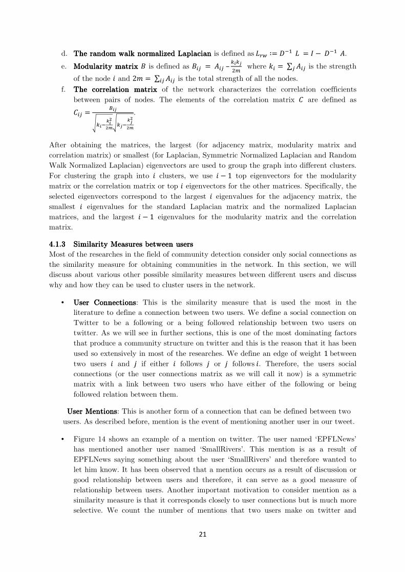
d. TTTThe random walk normalized Laplacianhe random walk normalized Laplacianhe random walk normalized Laplacianhe random walk normalized Laplacian is defined as��� ∶= ���� = � −����.
e. Modularity matrixModularity matrixModularity matrixModularity matrix � is defined as � = � – ������ where � =∑ � is the strength
of the node ! and 2# =∑ � is the total strength of all the nodes.
f. The correlation matrixThe correlation matrixThe correlation matrixThe correlation matrix of the network characterizes the correlation coefficients
between pairs of nodes. The elements of the correlation matrix $ are defined as
$ = %��&���'���(&���'�
��(
.
After obtaining the matrices, the largest (for adjacency matrix, modularity matrix and
correlation matrix) or smallest (for Laplacian, Symmetric Normalized Laplacian and Random
Walk Normalized Laplacian) eigenvectors are used to group the graph into different clusters.
For clustering the graph into ! clusters, we use ! − 1 top eigenvectors for the modularity
matrix or the correlation matrix or top ! eigenvectors for the other matrices. Specifically, the
selected eigenvectors correspond to the largest ! eigenvalues for the adjacency matrix, the
smallest ! eigenvalues for the standard Laplacian matrix and the normalized Laplacian
matrices, and the largest ! − 1 eigenvalues for the modularity matrix and the correlation
matrix.
4.1.34.1.34.1.34.1.3 Similarity Measures between usersSimilarity Measures between usersSimilarity Measures between usersSimilarity Measures between users
Most of the researches in the field of community detection consider only social connections as
the similarity measure for obtaining communities in the network. In this section, we will
discuss about various other possible similarity measures between different users and discuss
why and how they can be used to cluster users in the network.
• User User User User CCCConnectionsonnectionsonnectionsonnections: This is the similarity measure that is used the most in the
literature to define a connection between two users. We define a social connection on
Twitter to be a following or a being followed relationship between two users on
twitter. As we will see in further sections, this is one of the most dominating factors
that produce a community structure on twitter and this is the reason that it has been
used so extensively in most of the researches. We define an edge of weight 1between
two users ! and * if either ! follows * or * follows!. Therefore, the users social
connections (or the user connections matrix as we will call it now) is a symmetric
matrix with a link between two users who have either of the following or being
followed relation between them.
User MentionsUser MentionsUser MentionsUser Mentions: This is another form of a connection that can be defined between two
users. As described before, mention is the event of mentioning another user in our tweet.
• Figure 14 shows an example of a mention on twitter. The user named ‘EPFLNews’
has mentioned another user named ‘SmallRivers’. This mention is as a result of
EPFLNews saying something about the user ‘SmallRivers’ and therefore wanted to
let him know. It has been observed that a mention occurs as a result of discussion or
good relationship between users and therefore, it can serve as a good measure of
relationship between users. Another important motivation to consider mention as a
similarity measure is that it corresponds closely to user connections but is much more
selective. We count the number of mentions that two users make on twitter and

22
assign the weight of the link between two users ! and * as the total number of tweets
posted by ! that mention * and the tweets posted by * that mention the user!.
Figure 14: An example tweet showing a mention on twitter
• DescriptionDescriptionDescriptionDescription23232323 Content SimilarityContent SimilarityContent SimilarityContent Similarity: Users on twitter can post a description about
themselves which is shown in their profile. Figure 15 shows an example of description
on twitter for the user with screen name ‘pulkit110’. This description can sometimes
be used to measure the similarity between users on twitter. Since this description
generally describes the keywords about what the user likes to do or where he
works/studies at, it can serve as a very good suggestion of user similarity on twitter.
Therefore, we consider the cosine similarity between the users’ descriptions as one of
the similarity measures in determining the clusters of users on twitter.
Figure Figure Figure Figure 15151515: : : : Example of user description on Twitter
• Tweet Content SimilarityTweet Content SimilarityTweet Content SimilarityTweet Content Similarity: The most popular concept of twitter is the concept of
tweets. It is tweets that most users on twitter are interested in and therefore, it can
be used as a similarity measure between different users. We define the tweet
similarity between two users as the cosine similarity between the documents formed
by combining the tweets of a user into one. The text similarity measure between the
tweets helps us to observe if the users are interested in talking about similar topics. If
the users talk about the same topic then it is quite possible that they are interested
in similar things and is an indication of good similarity between them.
• HasHasHasHash tag similarity between usersh tag similarity between usersh tag similarity between usersh tag similarity between users: Hashtag is a unique concept on twitter which
allows users to specify important keywords in their tweets my prefixing ‘#’ before a
keyword in a tweet. Hashtags have been used on twitter to set trending topics as well
as start chat rooms etc. The hash tags allow users to specify what they think as an
important keyword in their tweet and therefore can be considered as a very strong
factor to compare two users’ similarity. Figure 16 shows an example of the user
‘diwakarsapan’ posting a tweet with hashtag ‘#IEUsers’. The hashtag shows that the
user wants to emphasize on a particular keyword in his tweet. We define the hash tag
similarity between two users as the cosine similarity between the collections of
hashtags of the different users.
23 Short text that user writes on his profile to describe himself

23
Figure Figure Figure Figure 16161616: : : : Example of hash tag on twitter
4.2.4.2.4.2.4.2. Results and Results and Results and Results and aaaanalysis on small datasetnalysis on small datasetnalysis on small datasetnalysis on small dataset
In this section we present an analysis of the spectral clustering algorithms for a small group
of users which are part of the larger group that we collected as described in section 2.3.3. For
this experiment, we use the following setup. We use three different user lists24 on twitter as
the ground truth data25 for the group of users. We obtained all the tweets from the users
who were listed in the three lists and then try to obtain clusters by using different matrices
(as described in section 4.1.2) using the spectral clustering algorithm. In addition to this, we
also explore different connections (similarity measures as described in section 4.1.3) between
users in addition to just the social connections in order to find out other features that affect
the users being listed together.
We now present the analysis of the clustering algorithms that we used to cluster the user
information from twitter. We present results of applying spectral clustering algorithm using
the modularity matrix (section 4.1.2.e) and the symmetric normalized Laplacian matrix
(section 4.1.2.c). We compare the results of these approaches while using several different
input matrices formed by different combination of the above similarity measures.
Figure 17 shows a spy plot26 of the user connections corresponding to the 501 users belonging
to the three different lists as mentioned above. The users have been ordered by the lists that
they belong to and therefore, we can immediately observe three communities present in the
network by looking at plot in Figure 17.
We try to find out this community structure using the spectral clustering algorithms. We
present the results of application of the algorithm on users’ social connections as well as
several other individual similarity measures (user mention similarity, description content
similarity and tweet content similarity) followed by a simple combination of the different
similarity measures. For finding the combined similarity measure, we sum all the different
similarity measures. Since the different similarity measures can be on different scales, these
similarity measures are normalized before we add them together and apply the clustering
algorithms. Therefore, the adjacency matrix that corresponds to the combined similarity
measures is the sum of all the individual normalized adjacency matrices.
In order to measure the accuracy of our clustering algorithms, we use several different cluster
evaluation objective functions to compare obtained clusters with the ground truth data of
clusters which represents the distribution of the users into different lists.
24 Lists are a way of grouping users on twitter. Users can follow lists to obtain updates from a group of users. 25 List ids: 4293757, 12932674 and 33222959 which correspond to the lists @prolificd/met, @rahulkalra_e/entrepreneurs and @8hasin/mildly-interesting respectively. 26 A plot that shows sparsity pattern of any matrix S.

24
Figure Figure Figure Figure 17171717: : : : Spy plot showing connections between the users ordered by lists that they belong to
We now present a brief description of the cluster evaluation functions that we use to
compare our results:
• Normalized Mutual Normalized Mutual Normalized Mutual Normalized Mutual InformationInformationInformationInformation: A normalized mutual information metric is a
mutual information metric whose range is normalized to [0,1].
+,�-., /0 = �-., /012-.02-/0 where �-0 is the mutual information metric and 2-0 is the entropy metric.
• Rand IndexRand IndexRand IndexRand Index: An alternative to the above information-theoretic interpretation of
clustering is to view it as a series of decisions, one for each of the pairs of documents
in the collection. We want to assign two documents to the same cluster if and only if
they are similar. A true positive (TP) decision assigns two similar documents to the
same cluster; a true negative (TN) decision assigns two dissimilar documents to
different clusters. There are two types of errors we can commit. A (FP) decision
assigns two dissimilar documents to the same cluster. A (FN) decision assigns two
similar documents to different clusters. The Rand index measures the percentage of
decisions that are correct. It penalizes both false positive and false negative decisions
during clustering.
3� = 45 6 4+45 6 75 6 4+ 6 7+
We compare our clustering results with the ground truth values for the different similarity
metrics as well as their combination. The results are presented in Table 1. Note that all
matrices have been normalized before applying the clustering algorithm. In addition to the
evaluation of the benchmark results for our data sets for the clustering algorithms, we also
present a few visualizations for the clustering results obtained on this small dataset in order
to better observe the accuracy of our clustering algorithms.

25
Figure 18 summarizes some of the results. The results have been obtained using Gephi27 for
visualization. The communities are represented by different colours in the visualizations.
Note that the arrangement of the nodes in the space doesn’t represent any communities. The
arrangement of nodes in the visualizations corresponds to a layout. We keep the same layout
for all the visualizations so that it is easy to see the results of the clustering process. The
different clusters in the visualizations are represented by different colours. This means that
all the nodes in the visualization that have the same colour have been placed into one cluster
for that visualization. Figure 18(a) shows the communities formed using the ground truth
data. Figure 18(b) shows the clusters obtained for the network using the user connections as
the only similarity measure using the modularity matrix for spectral clustering. Figure 18(c)
shows the results of community detection using the combination of all similarity measures
for the modularity matrix. Finally Figure 18(d) shows the results for community detection
applied on combined similarity measures using the Symmetric Normalized Laplacian matrix.
Table Table Table Table 1111: : : : Evaluation of clustering for small dataset
Similarity Similarity Similarity Similarity MatrixMatrixMatrixMatrix Modularity MatrixModularity MatrixModularity MatrixModularity Matrix
Symmetric Normalized Symmetric Normalized Symmetric Normalized Symmetric Normalized Laplacian Laplacian Laplacian Laplacian MatrixMatrixMatrixMatrix
NMI RI NMI RI
User Connections 0.3868 0.7174 0.0077 0.3374
Mention 0.0130 0.3398 0.0077 0.3374 Tweet content similarity 0.0074 0.3371 0.0077 0.3374
Description content Similarity
0.0780 0.5254 0.0088 0.3381
All combined 0.2500 0.6175 0.2931 0.6472
We can observe that user’s social connections are the most dominating factors for this group
of users while dividing the users into different communities. We can also observe that the
high values of benchmark results correspond to the good community detection that
corresponds closely to the ground truth data by looking at the visualizations in Figure 18(a)
and Figure 18(b) which show the ground truth clusters and the clusters obtained by
applying community detection using modularity matrix on social connections respectively.
The other individual similarity measures like the user mentions, tweet content similarity and
description content similarity don’t perform very well when used for community detection
using the modularity matrix. We also observe that the results for combined similarity
measures, i.e. the sum of connections, mentions, tweet content similarity and description
content similarity doesn’t perform as well as the connections. This means that the addition
of low information contents like the mentions, tweet content similarity and description
content similarity decreases the accuracy of the clustering algorithm even in the presence of
the highly informative social connections. A reason for the bad performance of the similarity
measures based on the tweets, descriptions and mentions can be that the group of users are
similar and generally post similar content on the web. This also means that the user
behaviours don’t seem to be consistent with the ground truth data.
27 Network analysis and visualization tool: www.gephi.org

26
(a) (b)
(c) (d)
Figure Figure Figure Figure 18181818: : : : Visualization results on small group. (a) Ground truth clusters (b) Clusters obtained using spectral clustering on modularity matrix for user connections (c) Clusters obtained using spectral clustering on modularity matrix for combined similarity measures (d) Clusters obtained using spectral clustering on symmetric normalized
Laplacian for combined similarity measures.
However, the detection of communities for the user’s social connections using the Symmetric
Normalized Laplacian matrix fails. This is because the Laplacian based methods are known
to be quite sensitive to the presence of disconnected nodes in the graph. Therefore, the
results of the social connections for the Symmetric Normalized Laplacian are similar to the
other individual results which mean that we are not able to reconstruct any valuable cluster
information when using the Normalized Laplacian. But the combined matrix performs
consistently even when using the Normalized Laplacian for community detection. This is
because addition of several different kinds of information to the social connections makes it a

27
connected graph and therefore, we now observe results consistent with the ones obtained
while using modularity matrix for community detection.
Therefore, we can conclude from these results that user connections are a very good measure
of information and for this model; they give the best clustering results when used with the
modularity matrix for spectral clustering. We can also see that adding several other non-
informative measures to this layer decreases the accuracy considerably when used with the
modularity matrix. However, an interesting observation occurs from our discussion and
results regarding the Symmetric Normalized Laplacian matrix that even a highly informative
layer (user connections) can prove to be a very bad indication of clustering if not used with
the correct clustering algorithm due to the presence of disconnected nodes in the graph. We
also found that even adding a non-informative (or slightly informative) layer as in this case
can improve the connectivity and therefore improve the clustering results.
4.3.4.3.4.3.4.3. Results and analysis on large datasetResults and analysis on large datasetResults and analysis on large datasetResults and analysis on large dataset
Let us now switch data set and move to a larger group of users. We now consider a group of
11273 users picked from the set of all the users collected in Section 2.3.3. Before we start
with the clustering on these sets of users, we again begin with a spy plot for the connections
between these users. As opposed to the previous spy plot (Figure 17), the users for this
group have not been arranged in any specific order as the ground truth clusters for this large
group of users is unknown to begin with. Figure 19 represents the spy plot for the
connections of the users. We can observe that the graph is sufficiently connected.
Figure Figure Figure Figure 19191919: : : : Spy plot of User Connections for 11273 users
Since we don’t know the number of clusters for the data set beforehand, we cannot apply the
spectral clustering algorithms (however, there have been a few researches on obtaining the
number of clusters form observing the eigenvalues of different matrices [2]). Therefore, we
will use an hierarchical clustering algorithm to obtain clusters for this dataset.

28
We have used the Fast Modularity community structure inference algorithm [3] to cluster
the users for the larger set. We use the algorithm on a weighted graph with the edge weights
representing a similarity measure. The algorithm uses an agglomerative approach to
maximize the modularity of the graph partitioning. Modularity [5] is a property of a network
and a specific proposed division of that network into communities. It measures how good a
partition is in the sense that there should be many edges within communities and very few
between them.
If we denote by � the similarity measure between the elements ! and * and suppose that
the elements are divided into communities such that vertex ! belongs to community 8, then
the fraction of edges that fall within communities, i.e. the edges that connect vertices in the
same community, is
∑ �9-8, 8 )∑ � = 1
2#:�9(8, 8
)
where 9(;, <) is 1 if ; = < and 0 otherwise and # = ��∑ � is the number of edges in the
graph. Note that we consider the graph to be symmetric and undirected. This measure is
large if the division for a graph is a good one meaning that the community structure is well
identified. But it cannot be used as a measure for evaluation of results as it attains its
maximum value when the complete graph is said to belong to one single community.
However, we can subtract the expected value of the same quantity in case of randomized
network in order to make it more meaningful. Let us define the degree of a vertex !by � to
be number of edges incident upon it. We then have the following:
� =:�
If we consider a randomized network, then the probability of an edge existing between
vertices ! and * would be ������ . Therefore, we can now define the modularity, > as
> = 12#:?� − ��2# @9(8, 8
)
We can now describe the simple modularity maximization algorithm. The algorithm works in
a greedy manner starting with each vertex in its own cluster and then repeatedly joins the
two communities whose amalgamation provides the maximum increase in the modularity.
We can see that the process will terminate after A − 1 such joins for a network of A vertices.
Let us define two more quantities in order to make the understanding of the algorithm
simpler.
BC� = 12#:D�E9(8, ;)9(8, <)
as the fraction of edges that join vertices in community ; to vertices in community <, and

29
FC = 12#:�9-8 , ;0
which is the fraction of edges that are attached to vertices in community ;. We can then
rewrite the equation for finding modularity, > as
> :-BCC � FC�0C
Now, if we consider our partitioned graph as a graph with one vertex representing each
community connected with other communities with a bundle of edges with the edges within
the community represented as self-loops, then the elements of the matrix for this modified
graph can be rewritten as �C�G 2#BC� and the joining of two communities ; and < can be
achieved by summing together the ;HI and <HI rows and columns. Another point to note
here is that the modularity can be increased only by merging the vertices having an edge
between them and therefore, we need to keep track of the change of modularity that can be
obtained by merging the vertices !and *only if they are in different communities and have
an edge between them in the original graph. We use the algorithm described in [3] in order
to speed up our community detection by maintaining a set of data structures for storingΔ>s.
Let us now analyse the results of the algorithm. Figure 20 presents the spy plot obtained
after rearranging the users based on the communities in which they were placed by our
algorithm when applied on the social connections matrix as the input. Note that we order
the clusters by the number of users in the cluster with the cluster with the most number of
users on the top. We can observe from the plot that the algorithm performs quite well in
arranging the users into different clusters. We obtain a modularity value of 0.650112 for the
final clustering result shown in the plot which corresponds to a very good community
structure between the users.
Figure Figure Figure Figure 20202020: : : : Connections between users arranged according to the clusters that they were assigned to

30
Figure 21: Visualization of communities obtained using Fast Modularity Community Detection on Users’ Social Connections
Figure 21 shows the results of applying community detection algorithm using users’ social
connections matrix as the only similarity measure between the users. Here, the different
colours represent the different clusters. We can observe that most of the nodes in the graph
are divided into 4 major communities with other small communities with very few nodes. In
fact the top 4 communities in the graph cover more than 93% of the total nodes. These
communities are represented by red, green, blue and purple colours in the decreasing order of
the nodes that they contain. Note that the positions of different nodes on the visualizations
don’t represent any cluster information about them. The positions of the nodes only
correspond to a layout. We keep a constant layout for all the different visualizations for this
group of users so that it is easy to draw conclusions by looking at the figures. We assign a
cluster label of 0, 1, 2 … to the clusters in the increasing order of their size.
By looking at the clusters detected by our community detection algorithm, we can see
several structures and draw inferences from the users in the clusters. E.g. the largest cluster,
(i.e. cluster 0) contains most of the users from UK. We also observe that the users are
mostly web developers/software developers/computer geeks and talk consistently about these
terms. In addition to this, an analysis of other clusters also shows several similarities
between the users in the same cluster. E.g. the users in cluster 2 talk mostly about
technologies like ‘Google’, ‘server’, ‘SQL’ etc. Figure 22 shows the tag cloud28 for the tweets
posted by the users from cluster 2. The tag cloud is built using the online service ‘Tag
Crowd’29. Note that the common words in English have been ignored while creating the tag
cloud. The tag cloud shows the common keywords in a larger font size. Hence, we can see
that most of the words that are very frequently used in the tweets are similar and are related
to technology.
28 A tag cloud or word cloud (or weighted list in visual design) is a visual depiction of user-generated tags, or simply the word content of a site, typically used to describe the content of web sites. 29 http://tagcrowd.com/

31
Figure Figure Figure Figure 22222222: : : : Tag cloud for tweets from cluster 2
If we look at the users in cluster labelled 4, we can see that most of the users are from the
same university in India, ‘International Institute of Information Technology, Hyderabad’30.
If we look at the users of cluster labelled 6, we can see that most of the users in this cluster
follow football. Most of the users that have been placed in the cluster are fans of Juventus
Football Club31.We can observe this through the description of a few users shown in Figure
23 as an example.
Figure Figure Figure Figure 23232323: : : : Descriptions of few users in cluster 6
Figure Figure Figure Figure 24242424: : : : Tag cloud for tweets from cluster 6
We can also observe from the tag cloud of the tweets from these users (as shown in Figure
24) that the users indeed talk a lot about football and also about ‘juventus’ which occurs as
an important keyword from the tag cloud. In addition to this, the other keywords are also
something which are related to football and games. This is what we would expect from the
tweets from one cluster that all the keywords from one cluster talk about similar things and
not something completely different. This also supports our claim that we should include
similarity measures other than the social connections in order to improve clustering results
because then we will be able to not only observe the clusters based on the users’ connections
but also on something that the users generally tweet about.
30 A few examples of such users have the user name ‘harithski’, ‘ravikishore’, ‘sairam’, ‘naveenkr’, ‘nageshwara’ etc. which have all been placed in the same cluster labelled 4. 31 A professional Italian association football club based in Turin, Piedmont

32
We now present results of community detection for the groups in order to visualize an
evolution of clusters in different weeks of data. Since connections of the users remain more or
less consistent throughout different weeks, we use other similarity measures in order to
divide the users into different communities. Our distribution would be mainly based on the
tweets that the users post on twitter. Therefore, we consider three similarity measures (in
addition to the social connections) that can be obtained by analysing the tweets that users
post on twitter. We use the tweet content similarity, user mentions as well as the hash tag
similarity between the users in order to divide them into different clusters for weekly data.
Note that there are several users who don’t tweet very often. E.g. For our data set, we find
that only 10-20% of the total users tweeted during the one month of data that we analyse
here. Therefore, there are several users for whom we don’t have any temporal information
and therefore it is difficult to apply clustering based on only that information (as there will
be several disconnected components in the network). We therefore take social connections
into account when applying community detection on weekly data.
(a) (b)
(c) (d)
Figure Figure Figure Figure 25252525: : : : Visualization of clusters for large dataset. (a) Communities obtained for Fast Modularity Detection on combination of Users’ Social Connections and Tweet content similarity, mentions and hash tag similarity for week 1 (b) Communities using the same kind of similarity measures for week 2 (c) Communities for week 3
(d) Communities for week 4

33
Figure 25 shows the results of applying the above community detection algorithm on the
group of 11273 users for a combination of different similarity measures for different weeks’
data. Figure 25(a) shows the communities obtained by combining other similarity measures
(tweet content similarity, user mentions and hash tag similarity) along with the users’ social
connections. The other similarity measures however are taken for only one week of data from
26th October, 2011 to 1st November 2011. This leads to a much finer distribution of users into
communities with the graph now divided into more than 7 considerably large clusters. We
show 7 different clusters in the graph with the colours red, green, blue, purple, cyan, dark-
red, dark-green and brown representing the different communities arranged according to
their size. Note that we keep the layout same so as to clearly see how the clusters evolve
over time.
We now present three additional visualizations with similar experimental settings for
different weeks of data. Figure 25(b) shows the communities obtained using data for the
week from 2nd November, 2011 to 8th November 2011 whereas Figure 25(c) and Figure 25(d)
show communities for 9th November 2011 to 16th November 2011 and 17th November 2011 to
23rd November 2011 respectively. The colour scheme remains the same with the colours
assigned according to the size of the communities. While transitioning from week 1 to week
2, we can clearly observe that how two communities (red and blue in Figure 25(a)) merged
together to form one cluster in the 2nd week but again split to their original configuration in
the 3rd week. We can observe some similar movements in the next three weeks but this time
between smaller communities.
We can also compare these results with the visualization from the clustering results for users’
social connections from Figure 21. We can see that the clustering on social connections lead
to formation of a cluster (as shown in blue colour in Figure 21) which was identified as a
combination of several small clusters as a result of applying the same algorithm after
employing temporal information along with social connections. This means that the temporal
information allowed us to make distinction between a group of users which were not very
tightly connected or who weren’t interested in similar topics. We can also see that the
division of the big cluster (in blue in Figure 21) into smaller clusters (in different colours in
Figure 25) remains consistent throughout the weekly results meaning that the division was
not a result of temporary fluctuations in the interests of the users and indeed points to a
logical division of users into different communities.
5555 Future mentions between userFuture mentions between userFuture mentions between userFuture mentions between userssss
In this section, we try to establish a relation between the mentions that users make on
twitter with other similarities between the users. First let us explore the reasons for which
the users might mention each other on twitter. We begin with the most obvious link between
the users that might result into a mention. This link is a social connection between the users
(either ! follows * or * follows!). If we consider twitter to be the only mode of
communication between the users, then we can assume that a user will mention another user
only when one of them sees the others’ tweets. And if we ignore the possibility of a user
searching for some keyword/topic and then mentioning a random user who writes something
interesting about the topic the other user is interested in. Therefore, we can assume with a

34
very good accuracy that the user mentions occur on twitter if two users are somehow
connected. Another factor for a user to mention another user would be if they have
mentioned each other in the past. This tends to point out that they have been having a
conversation and therefore share a good relation on twitter and therefore, are more likely to
mention each other in the future. Another reason for a user to mention another user on
twitter can be if he finds the other user’s tweets to be interesting. This similarity measure
between the users can be correctly monitored using the content similarity of the user tweets
and the hash tags. By saying this, we implicitly assume that a user also posts something that
he is interested in.
Therefore, we now have a good model that can correlate between the user mentions in the
future to the past data that we have obtained. Building a good model is the first step in
future link prediction, a topic of vast interest in the research community. However, we limit
our scope in this section to establishing a good relation between the mentions and other
similarity measures which is a starting point towards the more complex link prediction
problem. We now present the correlations between our similarity measures (tweet content
similarity, user mention similarity and hash tag similarity) calculated for the data in the
past with the mentions in the future.
The following results show the complete correlation matrix for the feature vectors obtained
for the users that have a social connection between them. For all the pair of users that have
a social connection between them, for the feature vectors by arranging the mentions between
these pairs of users in column 1, hash-tag similarity between these users in column 2, tweet
content similarity in column 3 followed by a weighted combination32 of these three similarity
measures in column 4.
We assign a weight of 5 to the hashtag similarity measure as it is one of the factors that
should have high correspondence with the future mentions between users on twitter. A main
reason for assigning high weight here is because it can be tracked easily by users on twitter
by using the twitter search feature or by seeing the trending topics. As we discussed earlier,
past mentions are another important factor for future mentions on twitter and therefore, we
assign a weight of 2 to these features. Tweet content similarity is one feature that users
cannot easily track on twitter and therefore we assign the minimum weight to this feature.
The column 5 contains the classes that we want to compare these features with. These
classes are obtained by using the mentions in the subsequent week with a class ‘1’ for a pair
of users that have a mention relationship between them (either ! mentions * or * mentions!) and class ‘0’ otherwise. We then find the correlations between different columns in the
matrix. The tables below summarize the results for the correlation coefficients for different
features. However, what is most interesting in the tables is the last column which shows the
correlation between the feature vectors and the future mentions.
Table 2 shows the results for correlation between the feature-vectors obtained in form data
for week 1 as compared to the mentions occurring in week 2(where the week boundaries are
same as described for Figure 25 in section 4.3) for a complete set of 11,273 users. As
discussed earlier, the most important property, i.e. past user mentions has a high correlation
32 Weighted combination = 2*Mention + 5*Hashtag + Tweet Similarity.

35
with the user mention data in the next week. This is as we expected because the users who
mention each other often are more likely to have a mention relationship in future than the
users who have not mentioned each other in the past. The next highest correlation with the
future mentions for the individual feature vectors is the hash-tag similarity. This is also in
line with our expectations as the users who tend to focus on the same keywords are more
likely to follow it with a conversation with each other on twitter which leads to mentions
between them. Therefore, the hash-tags are also quite good for modelling the future mentions
on twitter. The lowest correlation between the future user mentions is obtained for the
individual feature vector of tweet content similarity. The reason for this can be because it is
difficult to track tweets on twitter based on their content than it is using the hash-tags or
screen-names and therefore the tweets which have one of these features is more likely to start
a conversation between two users. The figure highlighted in Table 2 corresponds to the
correlation between our combined similarity measure w.r.t. the future mentions on twitter.
We see that it is slightly better than the individual information as it includes information
from two informative sources (i.e. the past mentions and the hash tag similarity).
Table Table Table Table 2222: : : : Correlation matrix for features and future mentions for feature vectors for week 1 as compared to mentions in week 2
W1/W2W1/W2W1/W2W1/W2 mention hash Tweet combined class
mention 1 0.0528 0.003 0.919 0.1656
hash 0.0528 1 0.0031 0.4422 0.0565
tweet 0.003 0.0031 1 0.0134 0.0272
combined 0.919 0.4422 0.0134 1 0.1713
class 0.1656 0.0565 0.0272 0.1713 1
Table 3 shows the results for the setting for data in week 1 and 2 as compared to the
mentions in week 3. We can observe some improvement in the results for the combined data
of two weeks as compared to only the first week’s data. From this, we can infer that we can
improve our results if we increase the data that we use to compute the feature vectors. Note
that here the combination of all the feature vectors doesn’t perform as well mention
individually. This is because of the low correlation of tweets and hash-tags which acts as a
noisy data in this example and therefore leads to a worse combined feature vector as
compared to the mention feature vector.
Table Table Table Table 3333: : : : Correlation matrix for features and future mentions for feature vectors for week 1 and week 2 as compared to mentions in week 3
W12/W3W12/W3W12/W3W12/W3 mention Hash tweet combined class
mention 1 0.0976 0.0003 0.8526 0.2186
Hash 0.0976 1 -0.0009 0.6033 0.0635
tweet 0.0003 -0.0009 1 0.008 0.0359
combined 0.8526 0.6033 0.008 1 0.2088
class 0.2186 0.0635 0.0359 0.2088 1
However, the results for Table 4 which show the correlation matrix for feature vectors for
weeks 1, 2 and 3 as compared to the future mentions in week 4 again show an improvement

36
in the correlation for combined feature vector. An interesting point to note here is that the
tweet content similarity feature vector has a negative correlation with the future mentions in
week 4. This means the tweet content similarity feature vector doesn’t correspond very well
to the mentions in the next week. However, we still see that the combined feature vectors
perform better than the past mentions and therefore we can say that the process of
combining the feature vectors can lead to better results.
Table Table Table Table 4444: : : : Correlation matrix for features and future mentions for feature vectors for week 1, 2 and 3 as compared to mentions in week 4
W123/W4W123/W4W123/W4W123/W4 mention hash tweet combined class
mention 1 0.1428 0.0219 0.8912 0.1906
hash 0.1428 1 0.0193 0.5761 0.0861
tweet 0.0219 0.0193 1 0.0343 -0.006
combined 0.8912 0.5761 0.0343 1 0.1968
class 0.1906 0.0861 -0.006 0.1968 1
The final correlation results that we show for the future mentions are obtained by
calculating the correlation for only a cluster of users. This group of users corresponds to the
users placed into the same cluster by using the Fast Modularity Maximization algorithm on
users’ social connections as explained in section 4.3. Table 5 shows the correlation matrix for
feature vectors for the users that belong to cluster 133. We can observe here that the results
are much better as compared to the previous results for the complete group of 11,273 users.
This is because the mentions are more likely to occur between the communities of users
rather than outside these communities. We can see that only one week’s data here surpasses
the previous results that use even more data. Another important observation that we can
make here is that the low correlation of tweets doesn’t act as too much of a noise in this case
as the correlations for the other two features are quite high as opposed to the previous cases.
This is another indication of how the cluster results obtained from the group of users can be
used to establish a relationship between different features on twitter.
Table Table Table Table 5555: : : : Correlation matrix for features and future mentions for feature vectors for week 1 as compared to mentions in week 2 calculated for only the users in cluster 1 (as obtained in section 4.3)
W1/W2W1/W2W1/W2W1/W2 mention hash tweet combined class
mention 1 0.0343 -0.0062 0.7492 0.1616
hash 0.0343 1 -0.0049 0.6876 0.2192
Tweet -0.0062 -0.0049 1 -0.0001 -0.0116
combined 0.7492 0.6876 -0.0001 1 0.2625
class 0.1616 0.2192 -0.0116 0.2625 1
6666 ConclusionConclusionConclusionConclusion & Future Work& Future Work& Future Work& Future Work
We proposed and described an approach to cluster users in twitter based on social
connections as well as content and link similarity. We analysed the performance of two
33 No. of users in the cluster: 2,128

37
standard clustering algorithms for clustering users in twitter and their variations. We also
explored different ways to improve the clustering results based on additional similarity
measures other than just the social connections. From our results and analysis, we conclude
that the social connections are no doubt a dominating factor in the community detection
process and play a major role in determining the communities in twitter. However, the other
similarity measures also perform quite well and can sometimes give us a finer idea of the
distribution of clusters when combined with the social connections. We found however, that
these other similarity measures are not suited to be used in absence of the social connections
mostly because of the lack of user interactions in a short period of time and the lack of
content distinctness when averaged over a long period of time. In our experiments and
clustering algorithms, we directly add the different similarity measures after normalizing
them to the same scale. However, we don’t consider different weights for the similarity
measures based on their importance. This is an approach that can be explored further in
order to improve the clustering results.
Towards the end, we also propose some reasons for the user mentions to occur on twitter.
We explore several different reasons for this event and also calculate the correlations
between the similarities between the tweet content, the past mentions and the hash tag
similarity in the preceding weeks to the event of mention in the subsequent weeks. We find
that the correlation improves as we take more data into consideration or calculate the
correlation for only the group of users that belong to one cluster. This shows that the cluster
results indeed identify some sort of a community structure as we would expect that the
mentions be confined within a community.
Here, we just present a brief discussion and a few arguments relating different similarity
measures to future mentions. The work can further be extended to achieve the solution to
the problem of future link prediction which has been gaining a lot of popularity in the
research. There have been quite a few researches to predict future links between scientists in
academia (based on co-authorship networks34) [14], Question-Answering Bulletin Boards35
[15] and twitter [16]. The prediction of future mentions between users on twitter can help to
better understand the community structure between users. Finally, we have limited our
discussions to very simple visualizations for the tweets collected based on keywords and
locations. We try to infer some conclusions and landmarks of interest from these
visualizations. However, in the future, the data can be used to automatically analyse the
tweets’ contents to achieve these goals.
7777 RRRReferenceseferenceseferenceseferences
[1] Chris Taylor, "Social networking 'utopia' isn't coming," CNN, 2011.
[2] Hua-Wei Shen and Xue-Qi Cheng, "Spectral methods for the detection of network
community structure: a comparative analysis," Journal of Statistical Mechanics: Theory
34 Networks that define collaboration between scientists based on whether they co-authored a paper 35 Questions are submitted on QABB and let somebody in the internet answer them. E.g. Yahoo! Answers

38
and Experiment, October 2010.
[3] M. E. J. Newman, and Cristopher Moore Aaron Clauset, "Finding community structure
in very large networks," Physical Review E, vol. 70, no. 6, 2004.
[4] Xiaowei Xu, Zhidan Feng Nurcan Yuruk, and Thomas A. J. Schweiger, "SCAN: A
Structural Clustering Algorithm for Networks," in 13 th ACM SIGKDD International
Conference on Knowledge Discovery and Data Mining, San Jose, 2007.
[5] M. Girvan and M. E. J. Newman, "Community structure in social and biological
networks," in National Acad. Sci. 99, 2002.
[6] A. Arenas, L. Danon, A. D´ıaz-Guilera, P.M. Gleiser, and R. Guimera, "Community
analysis in social networks," The European Physical Journal B, pp. 373–380, 2004.
[7] Takeshi Sakaki, Makoto Okazaki, and Yutaka Matsuo, "Earthquake shakes Twitter
users: real-time event detection by social sensors," in 19th international conference on
World wide web, Raleigh, North Carolina, USA, 2010, pp. 851--860.
[8] W. W. Zachary, "An information flow model for conflict and fission in small groups,"
Journal of Anthropological Research 33, pp. 452-473, 1977.
[9] Fredrik Espinoza et al., "Social and Navigational Aspects of Location-Based Information
Systems," Ubicomp 2001: Ubiquitous Computing, vol. 2201, pp. 2-17, 2001.
[10] Andranik Tumasjan, Timm O. Sprenger, Philipp G. Sandner, and Isabell M. Welpe,
"Predicting Elections with Twitter: What 140 Characters Reveal about Political
Sentiment," in Fourth International AAAI Conference on Weblogs and Social Media,
2010, pp. 178-185.
[11] S. Asur and B.A. Huberman, "Predicting the Future with Social Media," in 2010
IEEE/WIC/ACM International Conference on Web Intelligence and Intelligent Agent
Technology (WI-IAT), 2010, pp. 492 - 499.
[12] Rachael King. (2008, September) How Companies Use Twitter to Bolster Their Brands.
[13] W. E. Donath and A. J. Hoffman, "Lower bounds for the partitioning of graphs," IBM
Journal of Research and Development, pp. 420–425, 1973.
[14] David Liben-Nowell and Jon Kleinberg, "The Link Prediction Problem for Social
Networks," in 12th International Conference on Information and Knowledge
Management (CIKM), New Orleans, 2003, pp. 556--559.
[15] Tsuyoshi Murata and Sakiko Moriyasu, "Link Prediction of Social Networks Based on
Weighted Proximity Measures," in International Conference on Web Intelligence, 2007,
pp. 85-88.

39
[16] John Hopcroft, Tiancheng Lou, and Jie Tang, "Who Will Follow You Back? Reciprocal
Relationship," in CIKM 2011, 20th ACM Conference on Information and Knowledge
Management, Glasgow, Scotland, UK, 2011.