data management of extreme marine and coastal hydro ... faculteit/afdelingen... · ghahfaroki...

“paper-02” — 2008/6/29 — 12:02 — page 191 — #1

Journal of Hydraulic Research Vol. 46, Extra Issue 2 (2008), pp. 191–210

© 2008 International Association of Hydraulic Engineering and Research

Data management of extreme marine and coastal hydro-meteorological events

Gestion de données des événements hydrauliques-météorologiquesmarins et côtiersPIETER H.A.J.M. VAN GELDER, IAHR Member, Section of Hydraulic Engineering,Faculty of Civil Engineering and Geosciences, Delft University of Technology, The Netherlands. Stevinweg 1, 2628 CN Delft,P.O. Box 5048, 2600 GA DELFT, The Netherlands. Tel.: +31-15-2786544; +31-15-2785124;e-mail: [email protected] (author for correspondence)

CONG V. MAI, Section of Hydraulic Engineering, Faculty of Civil Engineering and Geosciences,Delft University of Technology, The Netherlands. Stevinweg 1, 2628 CN Delft, P.O. Box 5048, 2600 GA DELFT,The Netherlands. Tel.: +31 15 278 4735; fax: +31 15 278 5124; e-mail: [email protected]

WEN WANG, State Key Laboratory of Hydrology-Water Resources and Hydraulic Engineering, Hohai University,Nanjing, 210098, China. Tel.: +86-25-83787331; fax: +86-25-83786606; e-mail: [email protected]

GHAHFAROKI SHAMS, Section of Hydraulic Engineering, Faculty of Civil Engineering and Geosciences,Delft University of Technology, The Netherlands. Stevinweg 1, 2628 CN Delft, P.O. Box 5048, 2600 GA DELFT, The Netherlands.E-mail: [email protected]

MOHAMMAD RAJABALINEJAD, Section of Hydraulic Engineering, Faculty of Civil Engineering and Geosciences, DelftUniversity of Technology, The Netherlands. Stevinweg 1, 2628 CN Delft, P.O. Box 5048, 2600 GA DELFT,The Netherlands. Tel.: +31 (0) 15 27 85520; fax: +31 (0) 15 27 85124; e-mail: [email protected]

MADELON BURGMEIJER, Section of Hydraulic Engineering, Faculty of Civil Engineering and Geosciences,Delft University of Technology, The Netherlands. Stevinweg 1, 2628 CN Delft, P.O. Box 5048, 2600 GA DELFT,The Netherlands. Tel.: +31 15 27 89446; fax: +31 15 27 85124; e-mail: [email protected]

ABSTRACTIn statistical extreme value analysis and forecast modeling, data screening and management are necessary steps before fitting a probability distributionto represent adequately the observed data. These methods include trend analysis, steadiness tests, seasonality analysis, and long-memory studies; arecritically reviewed and applied to coastal datasets. It was shown that the smaller the timescale of the coastal process, the more likely it tends to benon-stationary. The seasonal variations in the autocorrelation structures are present for all the deseasonalized daily, 1/3-monthly and monthly coastalprocesses. The investigation of the long-memory phenomenon of coastal processes at different timescales shows that, with the increase of timescale,the intensity of long-memory decreases. Only the daily water level series exhibit a strong long-memory. Comparing the stationary test results and thelong-memory test results, these two types of tests are more or less linked, not only in that the test results have similar timescale patterns, but also inthat there is a general tendency that the stronger the nonstationarity, the more intense the long-memory.

RÉSUMÉDans l’analyse statistique et la prédiction des valeurs extrêmes, filtrer et gérer les données sont des étapes nécessaires avant d’ajuster une distributionde probabilité pour représenter de façon adéquate les données observées. Ces méthodes comprenant l’analyse de tendance, les tests de stabilité,l’analyse saisonnière et les études de mémoire à long terme sont revues de façon critique et appliquées à des jeux de données côtières. On montreque plus l’échelle de temps du procédé côtier est petite, plus il est probable qu’il soit non-stationnaire. Les variations saisonnières des structuresd’auto-corrélation sont présentes dans tous les procédés côtiers journaliers, tri-mensuels et mensuels desaisonnalisés. L’étude du phénomène demémoire à long terme des procédés côtiers à différentes échelles de temps montre que l’intensité de la mémoire à long terme diminue quand l’échellede temps augmente. Seul le niveau d’eau journalier montre une forte mémoire à long terme. En comparant les résultats des tests de stationnarité et demémoire à long terme, il apparait que les deux types de tests sont plus ou moins liés; non seulement les résultats des tests ont des modèles d’échellede temps similaires mais aussi, plus la non-stationnarité est forte, plus la mémoire à long terme tend à être intense.

Keywords: Data screening, extreme value analysis, long-memory study, seasonality analysis, steadiness test, trend analysis

Revision received September 21, 2007/ Open for discussion until December 31, 2008.

191

“paper-02” — 2008/6/29 — 12:02 — page 192 — #2

192 P.H.A.J.M. van Gelder et al. Journal of Hydraulic Research Vol. 46, Extra Issue 2 (2008)

1 Introduction

Probabilistic methods are used to design civil engineering struc-tures. The stress and load parameters are described by statisticaldistribution functions. The parameters of these functions are esti-mated by various methods. Of particular interest is the behaviorof each method for predicting the p-quantiles, i.e., the valuewhich is exceeded by the random variable with probability p,with p � 1. The estimation of extreme quantiles correspondingto a small probability of exceedance is commonly required in therisk analysis of hydraulic structures. Such extreme quantiles mayrepresent design values of environmental loads, including wind,waves, snow, and earthquakes; river discharges; and flood levelsspecified by design codes and regulations.

In civil engineering practice several estimation methods forprobability distribution functions are available, such as the:

— Method of moments,— Method of maximum likelihood,— Method of least squares (applied either on the original or on

the transformed data),— Method of Bayesian estimation,— Method of minimum cross entropy,— Method of probability weighted moments, and— Method of L-moments.

These methods were assessed relative to their performanceand critically reviewed by, e.g., van Gelder (1999). An investi-gation was made to determine which method is preferable forthe parameter estimation of a particular probability distributionfor a reliable estimate of the p-quantiles. Particular attention waspaid on the performance of the parameter estimation method withrespect to three criteria (i) based on the relative bias, (ii) RootMean Squared Error (RMSE), and (iii) based on the over- andunder-design.

It is desirable that the quantile estimate be unbiased, that isits expected value should be equal to the true value. It is alsodesirable that an unbiased estimate be efficient, i.e., its vari-ance be as small as possible. The problem of an unbiased andefficient estimation of extreme quantiles from small samples iscommonly encountered in civil engineering practice. For exam-ple, annual flood discharge data may be available for past 50–100years; on that basis one may have to estimate a design flood levelcorresponding to a 1000–10,000 years return period.

This work concentrates on the steps required before fittingan analytical probability distribution to represent adequately thesample observations. These steps involve the trend analysis,steadiness tests, a seasonality analysis, and long-memory studies.Then, the distribution type can be fitted from the data and param-eters of the selected distribution type can be estimated. Sincethe bias and the efficiency of quantile estimates are sensitive tothe distribution type, the development of simple and robust cri-teria for fitting a representative distribution to small samples ofobservations was an active area of research. van Gelder (1999)overviews such considerations. Herein, the issues on the trendanalysis are presented in Sec. 2, followed by steadiness testsin Sec. 3. Most environmental data show a seasonality behav-ior as discussed in Sec. 4. Section 5 is devoted to long memory

studies of environmental data. The proposed methods are appliedto test the coastal time series data at Noorwijk station at the DutchNorth Sea. The data were made available by the Dutch Ministryof Transport, Public Works and Water Management (RIKZ). Thedata of the period of 1979 to 2002 include wave heights, waveperiods and water levels.

2 Trend analysis

2.1 Introduction to trend analysis

Hydrological time series typically exhibit a trend behavior or non-steadiness. This behavior is a type of unsteadiness. In this presentstudy, they are treated separately. The purpose of a trend test is todetermine whether the values of a series have a general increaseor decrease with time, whereas the purpose of a stationarity testis to determine if the distribution of a series depends on the time.

An important task in the hydrological modeling is to determineif the data have a trend and how to achieve stationarity when thedata is nonstationary. The possible effects of global warmingon the water resources were recently investigated (e.g., Letten-maier and Wood, 1993; Jain and Lall, 2001; Kundzewicz et al.,2004; Wang, 2006). Thus, detecting the trend and stationarity ina hydrological time series may help to understand the possiblelinks between hydrological processes and changes in the globalenvironment. The focus of the trend analysis and stationarity testin this study is not to detect the changes of regional or world-widestreamflow processes. As a matter of fact, the presence of trendsand nonstationarity is undesirable in the further analysis. There-fore, one should make sure whether there is both a trend and anonstationarity or not, and if yes, the appropriate pre-processingprocedure should be applied. The issue of trend analysis is there-fore studied, whereas the nonstationarity problem is addressed inthe next section.

Non-parametric trend detection methods are less sensitive tooutliers (extremes) than are parametric statistics, such as Pear-son’s correlation coefficient. In addition, a nonparametric testcan determine a trend in a time series without specifying whetherthe trend is linear or nonlinear. Therefore, the rank-based non-parametric Mann-Kendall’s test (Kendall, 1938; Mann, 1945) isapplied to annual and monthly coastal time series.

2.2 Trend test for annual coastal time series data

First, the trend of annual series is tested to obtain an overall viewof the possible changes in coastal time series data.

2.2.1 Mann-Kendall testKendall (1938) proposed a quantity τ (tau) to measure the strengthof the monotonic relationship between two variables x and y.Mann (1945) suggested to use the test for the significance ofKendall’s tau where one of the variables is time as a test fora trend. This test is known as the Mann-Kendall (MK) test,which is powerful for discovering deterministic trends. Underthe null hypothesisH0, that a series {x1, . . . , xN} originates froma population where the random variables are independent and

“paper-02” — 2008/6/29 — 12:02 — page 193 — #3

Journal of Hydraulic Research Vol. 46, Extra Issue 2 (2008) Data management of extreme marine and coastal hydro-meteorological events 193

identically distributed, the MK test statistic states

S =N−1∑i=1

N∑j=i+1

sgn(xj − xi), where

sgn(x) =

+1, x > 00, x = 0

−1, x < 0(1)

with

τ = 2S

N(N − 1)(2)

Kendall (1975) demonstrated that the variance of S, Var(S), forthe situation where there may be equal x values, is given by

σ2s = 1

18

[N(N − 1)(2N + 5)−

m∑i=1

ti(ti − 1)(2ti + 5)

](3)

where m is the number of the tied groups in the data set and tiis the number of data points in the ith tied group. Under the nullhypothesis, the quantity z is approximately standard normallydistributed even for the sample size N = 10, namely

z =(S − 1)/σs if S > 00 if S = 0(S + 1)/σs if S < 0

. (4)

It was found that the positive serial correlation inflates thevariance of the MK statistic S and hence increases the possibilityof rejecting the null hypothesis of no trend (von Storch, 1995). Toreduce the impact of serial correlations, it is common to prewhitenthe time series by removing the serial correlation from the seriesthrough yt = xt−φxt−1, where yt is the prewhitened series value,xt the original time series value, and φ the estimated lag 1 serialcorrelation coefficient. The pre-whitening approach was adoptedin many trend-detection studies (e.g., Douglas et al., 2000; Zhanget al., 2001; Burn and Hag Elnur, 2002).

2.2.2 MK test resultsThe first step in a time series analysis is a visual data inspection.Significant changes in the level or slope usually are obvious. Theannual average wave height, the water level and the wave periodseries of the Noordwijk location are shown in Fig. 1. It seems that

80

85

90

95

1979 1981 1983 1985 1987 1989 1991 1993 1995 1997 1999 2001 2003 2005

110130150170

1979 1981 1983 1985 1987 1989 1991 1993 1995 1997 1999 2001 2003 2005

47

48

4950

51

52

1979 1981 1983 1985 1987 1989 1991 1993 1995 1997 1999 2001 2003 2005

Figure 1 Annual water level (cm), wave height (cm), wave period (0.1 s)series of Noordwijk data set

Table 1 Mann-Kendall tests on annual series

Series Nonmiss tau t-Stat MK-Stat p-value

Wave Height 24 0.0507 14 0.347 0.728Water Level 24 0.4420 122 3.026 0.002Wave Period 24 0.0725 20 0.496 0.620

for the annual wave series there is no clear trend, while a slightupward trend is present for the water level. The MK test result isdisplayed in Table 1.

2.3 Trend test for monthly coastal time series

The trend test for annual series gives an overall view of thechange in coastal time series processes. To examine possiblechanges over to smaller timescale, the monthly coastal seriesneed to be investigated. Monthly coastal data usually exhibitstrong seasonality. The trend test techniques for dealing with sea-sonality of univariate time series fall into three major categories(Helsel and Hirsch, 1992): (1) Fully nonparametric method, i.e.,seasonal Kendall test, (2) Mixed procedure, i.e., regression ofde-seasonalized series on time, and (3) Parametric method, i.e.,a regression of original series on time and seasonal terms. Theseasonal Kendall test will be used here.

2.3.1 Seasonal Kendall testHirsch et al. (1982) introduced a modification of the MK test,referred to as the seasonal Kendall test that allows for seasonalityin observations collected over time by computing the Mann-Kendall test of each of p seasons separately, and then combiningthe results. Compute the following overall statistic S′

S′ =p∑j=1

Sj, (5)

where Sj is simply the S-statistic in the MK test for season jwith j = 1, 2, . . . , p, see Eq. (1). When no serial dependence isexhibited in the time series, the variance of S′ is defined as

σ2S′ =

p∑j=1

Var(Sj). (6)

When a serial correlation is present, as in the case of monthlytime series processes, the variance of S′ is defined as (Hirsch andSlack, 1984)

σ2S′ =

p∑j=1

Var(Sj)+p−1∑g=1

p∑h=g+1

σgh, (7)

where σgh denotes the covariance between the MK statistic forseason g and the MK statistic for season h. The covariance isestimated with the following procedures. Let the matrix

X =

x11 x12 · · · x1p

x21 x22 · · · x2p...

......

xn1 xn2 · · · xnp

(8)

“paper-02” — 2008/6/29 — 12:02 — page 194 — #4


denote a sequence of observations taken over p seasons for nyears. Let the matrix

R =

R11 R12 · · · R1p

R21 R22 · · · R2p...

......

Rn1 Rn2 · · · Rnp

(9)

denote the ranks corresponding to the observations in X, wherethe n observations for each season are ranked among themselves,that is

Rij = 1

2

[n+ 1 +

n∑k=1

sgn(xij − xkj)

]. (10)

Hirsch and Slack (1984) suggest to estimate σgh if there areno missing values (Dietz and Killeen, 1981)

σgh = 1

3

[Kgh + 4

n∑i=1

RigRih − n(n+ 1)2], (11)

where

Kgh =n−1∑i=1

n∑j=i+1

sgn[(Xjg −Xig)(Xjh −Xih)]. (12)

If there are missing values, then

Rij = 1

2

[nj + 1 +

nj∑k=1

sgn(Xij −Xkj)

], (13)

wherenj is the number of observations without missing values fora season j. The covariance between the MK statistic for seasong and season h is

σgh = 1

3

[Kgh + 4

n∑i=1

RigRih − n(ng + 1)(nh + 1)

](14)

Table 2 Seasonal Kendall tests on monthly series

Series Nonmiss Test Stat τau Std. Dev. MK-Stat p-value

Wave Height 288 153 0.004 129.835 1.178 0.2386Water Level 288 628 0.0152 229.603 2.735 0.006Wave Period 288 −16 −0.0004 139.23 −0.108 0.914

Table 3 Mann-Kendall tests for each month

Month Jan Feb Mar Apr May Jun Jul Aug Sep Oct Nov Dec

(a) Wave heightτau −0.116 0.384 0.007 −0.007 0.261 0.174 0.123 −0.181 0.072 0.12 −0.159 −0.123MK-Stat −0.794 2.629 0.05 −0.05 1.786 1.191 0.843 −1.24 0.496 0.819 −1.091 −0.843p-value 0.564 0.555 0.547 0.539 0.531 0.522 0.514 0.506 0.498 0.473 0.481 0.399

(b) Water levelτau 0.036 0.362 0.254 0.261 0.366 0.254 0.261 0.123 0.174 0.109 0.196 −0.119MK-Stat 0.248 2.48 1.736 1.786 2.506 1.737 1.786 0.843 1.191 0.744 1.339 −0.819p-value 0.804 0.013 0.083 0.074 0.012 0.082 0.074 0.399 0.234 0.457 0.18 0.413

(c) Wave periodτau −0.123 0.315 0.058 0.12 0.105 0.04 −0.098 −0.174 −0.01 0.011 −0.163 −0.137MK-Stat −0.843 2.159 0.397 0.819 0.72 0.273 −0.67 −1.191 −0.05 0.074 −1.117 −0.943p-value 0.399 0.031 0.691 0.413 0.472 0.785 0.503 0.234 0.96 0.941 0.264 0.346

Then the quantity z′ is approximately standard normallydistributed, namely

z′ =(S′ − 1)/σS′ if S′ > 00 if S′ = 0(S′ + 1)/σS′ if S′ < 0

. (15)

The overall tau is the weighted average of the p seasonal τ’s,defined as

τ =p∑j=1

njτj

/p∑j=1

nj, (16)

where τj is the tau for season j, estimated with Eq. (2). Theseasonal Kendall test is appropriate for testing for trend of eachseason when the trend is always in the same direction acrossall seasons. However, the trend may have different directions indifferent seasons. van Belle and Hughes (1984) suggested to testfor heterogeneity in trend

χ2het =

p∑j=1

z2j − pz2, (17)

where zj denotes the z-statistic for the jth season, computed as

zj = Sj

(Var(Sj))1/2, (18)

and

z = 1

p

p∑j=1

zj. (19)

Under the null hypothesis of no trend in any season, the statis-tic defined in Eq. (17) is approximately distributed as a chi-squarerandom variable with p− 1 degrees of freedom.

“paper-02” — 2008/6/29 — 12:02 — page 195 — #5


2.3.2 Seasonal Kendall test resultsThe monthly water level, wave height, and wave period timeseries data are tested for the trend with the seasonal Kendall testwhich allows for the serial dependence. The heterogeneity intrend is also tested. The results are shown in Table 2. The trendof coastal data at Noordwijk location of each month is furtherinvestigated with the MK test (Table 3).

3 Stationarity test

3.1 Test methods

In most applications of hydrological and oceanic modelling, theassumption of stationarity is made. It is thus necessary to test it.Sometimes the investigation of nonstationarity may give insightinto the underlying physical mechanism, especially in the con-text of global changes. Therefore, testing for stationarity is animportant topic in the field of environmental data.

There are roughly two groups of methods for testing sta-tionarity. The first group is based on the analysis of statisticaldifferences of different segments of a time series (e.g., Chen andRao, 2002). If the observed variations in a certain parameterof different segments are found to be significant, i.e., outside theexpected statistical fluctuations, the time series is considered non-stationary. Another group of stationarity tests is based on statisticsfor the full sequence, which was adopted in the following.

The stationarity test is carried out with two methods in thispresent study. The first relates to the augmented Dickey–Fuller(ADF) unit root test proposed by Dickey and Fuller (1979) andmodified by Said and Dickey (1984). It tests for the presence ofunit roots in the series (difference stationarity). The second is theKPSS test of Kwiatkowski et al. (1992), which tests for stationar-ity I stop here with marking “stationarity” around a deterministictrend (trend stationarity) and the stationarity around a fixed level(level stationarity). The KPSS test can also be modified to a unitroot test, but Shin and Schmidt (1992) demonstrated that theKPSS statistic, designed for a test for stationarity, was not asgood a unit root test as other standard tests. In particular, itspower is noticeably smaller than of the Dickey–Fuller, or othersimilar tests against stationary alternatives.

3.1.1 ADF testThe Dickey–Fuller unit-root tests are conducted through theordinary least squares (OLS) estimation of regression modelsincorporating either an intercept or a linear trend. Consider theAuto-Regressive (AR) (1) model

xt = ρxt−1 + εt, t = 1, 2, . . . , N, (20)

where x0 = 0; |ρ| ≤ 1 and εt is a real valued sequence ofindependent random variables with mean zero and variance σ2.If ρ = 1, the process {xt} is nonstationary and it is known as arandom walk process. In contrast, if |ρ| < 1, the process {xt} isstationary. The maximum likelihood estimator of ρ is the OLSestimator

ρ =(

N∑t=2

x2t−1

)−1 N∑t=2

xtxt−1. (21)

Under the null hypothesis ρ = 1, Dickey and Fuller (1979)showed that ρ is characterized by

N(ρ − 1) = N∑N

t=2(xtxt−1 − x2t−1)∑N

t=2 x2t−1

D−→ �2 − 1

2�, (22)

where

(�,�) =( ∞∑i=1

γ2i Z

2i ,

∞∑i=1

21/2γiZi

), (23)

with

γi = 2(−1)i+1/[(2i− 1)π], (24)

and the Zi are i.i.d. (independent and identically distributed)N(0,1) distributed random variables. The result of Eq. (22) allowsthe point estimate ρ to be used by itself to test the null hypothe-sis of a unit root. Another popular statistic for testing the nullhypothesis ρ = 1 is based on the usual OLS t-test of thishypothesis,

t = ρ − 1

σρ, (25)

where σρ is the usual OLS standard error for the estimatedcoefficient,

σρ = se

(N∑t=2

x2t−1

)−1/2

, (26)

and se denotes the standard deviation of the OLS estimate of theresiduals in the regression model with Eq. (20), estimated as

s2e = 1

N − 2

N∑t=2

(xt − ρxt−1)2. (27)

Dickey and Fuller (1979) derived the limiting distribution of thestatistic t under the null hypothesis that ρ = 1 as

tD−→ 2�−1/2(�2 − 1). (28)

A set of tables of the percentiles of the limiting distributionof the statistic t under ρ = 1 is available (Fuller, 1976). The testrejects ρ = 1 when t is “too negative”.

The unit root test described above is valid if the time series{xt} is well characterized by an AR(1) with white noise errors.Many hydrological time series, however, have a more compli-cated dynamic structure than is captured by a simple AR(1)model. The basic autoregressive unit root test can be augmented(referred to as ADF test) to accommodate the general ARMA(p, q) models with unknown orders (Said and Dickey, 1984;Hamilton, 1994). A brief description of the ARMA type modelis given in Appendix 2. The ADF test is based on estimating thetest regression

xt = βDt + φxt−1 +p∑j=1

ψj∇xt−j + εt, t = 1, 2, . . . , N,

(29)

whereDt is a vector of deterministic terms. The p lagged differ-ence terms, ∇xt−j , are used to approximate the ARMA structureof the errors, and the value of p is set so that the error εt is

“paper-02” — 2008/6/29 — 12:02 — page 196 — #6


serially uncorrelated. Said and Dickey (1984) show that theDickey–Fuller procedure, which was originally developed forautoregressive representations of known order, remains validasymptotically for a general ARIMA (p, 1, q) process in whichp and q are unknown orders.

3.1.2 KPSS testLet {xt}, t = 1, 2, . . . , N, be the observed series for which wewish to test stationarity. Assume that the series can be decom-posed into the sum of a deterministic trend, a random walk, anda stationary error with the following linear regression model

xt = rt + βt + εt (30)

where rt is a random walk, i.e., rt = rt−1 + ut , and ut is i.i.d.N(0, σ2

u), βt is a deterministic trend, and εt is a stationary error. Totest in this model if xt is a trend stationary process, namely, if theseries is stationary around a deterministic trend, the null hypoth-esis will be σ2

u = 0, meaning that the intercept is a fixed element,against the alternative of a positive σ2

u . In another stationaritycase, the level stationarity, namely, the series is stationary arounda fixed level, the null hypothesis will be β = 0. Under the nullhypothesis, for trend stationary, the residuals et(t = 1, 2, . . . , N)are from the regression of x on an intercept and time trendet = εt; whereas for level stationarity, the residuals et are from aregression of x on intercept only, that et = xt − x.

Let the partial sum process of et be

St =t∑

j=1

ej, (31)

and σ2 be the long-run variance of et , defined as

σ2 = limN−1E[S2N

]. (32)

The consistent estimator of σ2 can be constructed from theresiduals et by (Newey and West, 1987)

σ2(p) = 1

N

N∑t=1

e2t + 2

N

p∑j=1

wj(p)

N∑t=j+1

etet−j, (33)

where p is the truncation lag, wj(p) an optional weighting func-tion that corresponds to the choice of a special window, e.g., theBartlett (1950) window wj(p) = 1 − j/(p+ 1). Then the KPSStest statistic is

KPSS = N−2N∑t=1

S2t

/σ

2(p). (34)

Under the null hypothesis of level stationarity

KPSS →∫ 1

0V1(r)

2 dr, (35)

where V1(r) is a standard Brownian bridge V1(r) = B(r) – rB(1)and B(r) is a Brownian motion process on r ∈ [0, 1]. Under thenull hypothesis of trend stationary

KPSS →∫ 1

0V2(r)

2 dr (36)

where V2(r) is the second level Brownian bridge

V2(r) = B(r)+ (2r − 3r2)B(1)+ (−6r + 6r2)

∫ 1

0B(s) ds

(37)

Table 4 Upper tail critical values for the KPSS test statistic asymptoticdistribution

Distribution Upper tail percentiles

0.1 0.05 0.025 0.01∫ 1

0V1(r)

2 dr 0.347 0.463 0.574 0.739

∫ 1

0V2(r)

2 dr 0.119 0.146 0.176 0.216

The upper tail critical values of the asymptotic distribution ofthe KPSS statistic are listed in Table 4, as given by Kwiatkowskiet al. (1992).

3.2 Results of stationarity test results

Because both the ADF and the KPSS tests are based on thelinear regression, which assumes a normal distribution, a log-transformation can convert an exponential trend possibly presentin the data into a linear trend. Therefore, it is common to takelogs of the data before applying theADF and the KPSS tests (e.g.,Gimeno et al., 1999). In this study, the coastal time series of waterlevels, wave heights and wave periods are log-transformed beforethe doing stationarity tests.

An important practical issue for the implementation of thesetwo tests is to specify the truncation lag values of p in Eqs (29)and (33). The KPSS test statistics are fairly sensitive to the choiceof p, and for every series the value of the test statistic decreasesas p increases (Kwiatkowski et al., 1992). If p is too small thenthe remaining serial correlation in the errors will bias the testtoward rejecting the null hypothesis. If p is too large then thepower of the test will suffer. The larger the p, the less likely isthe null hypothesis to be rejected. Following Schwert (1989) andKwiatkowski et al. (1992), the number of lag length is subjec-tively chosen as p = int[x(N/100)1/4], with x = 4 in the presentstudy for coastal processes from monthly to daily timescales. Forannual series p = 1, because the autocorrelation at lag one isvery low, so it is generally enough to exclude the serial correla-tion. The function unitroot and stationaryTest implemented in theS + FinMetrics version 1.0 (Insightful Corporation, 2001; Zivotand Wang, 2002) are used to do the ADF test and the KPSS test.

The test results for the coastal data at Noordwijk location showthat, except for daily water level time series which is not station-ary, all the other time series appear to be stationary at a 5%significant level, since the unit root hypothesis with ADF test at1% significance level cannot be accepted, nor reject the trendstationarity hypothesis with KPSS test mostly at the 5% level.For the other time series of wave height and wave period thehypothesis of level stationary and trend stationarity is rejected bythe KPSS test or just accepted at a low significance level. Thehypothesis of the level stationary is accepted for the monthly,1/3-monthly, and the annual water level time series. Therefore, itcan be supposed that only the daily time series of the water levelis not stationary. One of the reasons of this nonstationarity canbe the daily fluctuation of the water level.

“paper-02” — 2008/6/29 — 12:02 — page 197 — #7


Two issues should be noticed. Firstly, although no significantcycle with a period longer than one year is detected using spectralanalysis for any coastal time series in this study, as will be seen inSec. 4, coastal processes normally exhibit seasonality. Therefore,they have periodic stationarity, rather than “normal” stationarity.According to Table 5, the KPSS test is not powerful enough todistinguish the periodic stationarity from the “normal” station-arity. Secondly, it is not clear how the presence of seasonalityimpacts the test of stationarity. Besides testing for nonstationarityin log-transformed series, the stationarity for the de-seasonalizedcoastal time series was also tested. The deseasonalization is con-ducted by taking first a log-transformation of the original dataset, then subtracting the seasonal (i.e., the daily, 1/3-monthlymonthly, or yearly) mean values and dividing by seasonal stan-dard deviations. The results are presented in Table 6, showing thatall the test results are generally larger for the KPSS test and “lessnegative” forADF test. In consequence, thep-values decrease for

Table 5 Stationarity test results for log-transformed coastal series

Series Lag max KPSS level stationary KPSS trend stationary ADFunit root

Results p-value Results p-value Results p-value

Daily WL 4 0.1981∗ <0.05 2.297∗∗ <0.01 −24.59 6.598e-90Hs 4 0.0644 >0.01 0.1146 >0.01 −20.35 1.623e-69Tp 4 0.1045 >0.01 0.1061 >0.01 −22.06 4.828e-78

1/3-montly WL 2 0.0451 >0.01 0.2877 >0.01 −8.333 6.104e-13Hs 2 0.034 >0.01 0.0546 >0.01 −10.23 2.788e-19Tp 2 0.0966 >0.01 0.0996 >0.01 −9.594 4.442e-17

Monthly WL 2 0.0199 >0.01 0.046 >0.01 −10.41 1.896e-17Hs 2 0.0282 >0.01 0.0369 >0.01 −9.074 7.512e-14Tp 2 0.0854 >0.01 0.0977 >0.01 −9.143 4.929e-14

Anual WL 1 0.0867 >0.01 0.1223 >0.01 −3.551 0.05834Hs 1 0.0819 >0.01 0.3142 >0.01 −3.812 0.03539Tp 1 0.1441 >0.01 0.1769 >0.01 −3.339 0.08612

Notes: ∗Significant at 5% level = data may not be stationary at p < 5%.∗∗Significant at 1% level = data may not be stationary at p < 1%.

Table 6 Stationarity test results for log-transformed, de-seasonalized coastal data

Series Lag KPSS level stationary KPSS trend stationary ADF unit root

Results p-value Results p-value Results p-value

Daily WL 4 0.05 > 0.01 1.0945∗∗ < 0.01 −23.9 8.933e-87Hs 4 0.0474 > 0.01 0.1747 > 0.01 −23.7 8.337e-86Tp 4 0.1213 > 0.01 1.4921∗∗ < 0.01 −24.21 3.509e-88

1/3-montly WL 2 0.0365 > 0.01 0.2307 > 0.01 −8.386 1.537e-14Hs 2 0.0303 > 0.01 0.0485 > 0.01 −7.974 7.81e-12Tp 2 0.0823 > 0.01 0.0849 > 0.01 −8.378 4.463e-13

Monthly WL 2 0.0199 > 0.01 0.046 > 0.01 −10.41 1.896e-17Hs 2 0.0282 > 0.01 0.0369 > 0.01 −9.074 7.513e-14Tp 2 0.0854 > 0.01 0.0977 > 0.01 −9.143 4.929e-14

Anual WL 1 0.0829 > 0.01 0.1389 > 0.01 −5.54 0.001004Hs 1 0.0866 > 0.01 0.1759 > 0.01 −3.004 0.1531Tp 1 0.1263 > 0.01 0.1328 > 0.01 −2.675 0.2548

Notes: ∗Significant at 5% level = data may not be stationary at p < 5%.∗∗Significant at 1% level = data may not be stationary at p < 1%.

the KPSS test, indicating an increase of the probability of reject-ing the hypothesis of stationary, and an increase for the ADF test,indicating the increase of the probability of accepting the hypoth-esis of unit root. That is, the removal of seasonality in the meanand variance tends to make the time series less stationary, at leastfor the KPSS test. This is an issue open for future investigation.

4 Seasonality analysis

4.1 Seasonality in mean and variance

The dynamics of natural processes such as wind driven coastalprocesses including the variation of water level, wave heights andwave periods are often dominated by annual variations (Fig. 1).The quality of capturing the seasonality is an important crite-rion for assessing a stochastic model for these processes. Theseasonality of hydro-meteorological processes is often described

“paper-02” — 2008/6/29 — 12:02 — page 198 — #8


in terms of the mean values, the variances, the extremes, andthe probability distribution of the variable in each season. In thefollowing the daily coastal series is used for the seasonality anal-ysis. This can be easily adapted to the 1/3-monthly or to monthlyseries.

For convenience to analyze the seasonality of a coastal dataseries of N years, the data are arranged in the matrix form as

X =

x1,1 x1,2 · · · x1,365

x2,1 x2,2 · · · x2,365...

... xj,i...

xN,1 xN,2 · · · xN,365

, (38)

where the rows denote year 1 ∼N, and the columns denote day1 ∼ 365. For simplicity, the 366th days of leap years are omitted.This would not introduce major errors when analyzing season-ality of the daily variation of the water level, the wave heightand the wave period. Consequently, the mean value, the standarddeviation and the coefficient of variation of each column of thematrix are the daily mean of the water level, the wave heightand the wave period, the standard deviation and the coefficient ofvariation (CV) of these daily data for each day over a year. Theyare easily calculated as

Mean value : xi = 1

N

N∑j=i

xj,i (39a)

Standard deviation : si = 1

N − 1

N∑j=1

(xj,i − xi)2

1/2

(39b)

Coefficient of variation : CV i = si

xi(39c)

The daily variations of mean, standard deviations and CVs ofwater level WL, the significant wave heightHs and the peak waveperiod Tp of North Sea at Noordwijk location are shown in Figs 2to 4. It is clear that days with high mean values have also highstandard deviations, a property well recognized (e.g., Mitosek,

0 50 100 150 200 250 300 350

80

100

120Daily mean variation

day

Wat

er le

vel(m

)

0 50 100 150 200 250 300 3500

50

Daily standard variation

day

Wat

er le

vel(m

)

0 50 100 150 200 250 300 3500

0.5

1Daily CV variation

day

CV

(-)

Figure 2 Seasonal variations in daily mean, standard deviation andcovariance of water level

0 50 100 150 200 250 300 350

100

200

Daily mean variation

day

Wav

e he

ight

(m)

0 50 100 150 200 250 300 3500

50

100

150Daily standard variation

day

Wav

ehe

ight

(m)

0 50 100 150 200 250 300 3500

0.5

1Daily CV variation

day

CV

(-)

Figure 3 Seasonal variations in daily mean, standard deviation and CVsof wave heights

0 50 100 150 200 250 300 350

0 50 100 150 200 250 300 350

0 50 100 150 200 250 300 350

40

50

60Daily mean variation

day

Wav

e pe

riod(

s)

0

10

20Daily standard variation

day

Wav

e pe

riod(

s)

0

0.2

0.4Daily CV variation

day

CV

(-)

Figure 4 Seasonal variations in daily mean, standard deviation and CVsof wave periods

2000). As a consequence, it has a similar seasonal pattern in theCVs too, as shown in the same figure. For all three data sets, theresults show that the seasons with high mean, standard deviationand CV’s are between the months October and March. This isexplained by the fact that this period corresponds to the winterseason when large wind speeds and therefore surges leading tohigher water levels and wave heights are expected. The highestcoastal values are found around mid February and the end ofDecember, which roughly equates to the time of the equinoxeswhen the largest tides of the year occur.

4.2 Detrending, normalization and de-seasonalization

After the trend and the seasonality analyses, the trend and theseasonal components can be removed from the original coastaldata series, to give an approximately stationary process. Furtherthe analysis of the autocorrelation and long-memory propertiescan be performed.

“paper-02” — 2008/6/29 — 12:02 — page 199 — #9


Because coastal data series are skewed and heavily tailed,whereas many models such as the regression or the autoregressivemoving average (ARMA) models require the time series data tobe normally distributed, it is necessary to normalize the data tomake them at least approximately normally distributed. The mostpopular approach is the Box–Cox transformation (Box and Cox,1964)

x ={λ−1[(x+ c)λ − 1] λ = 0ln(x+ c) λ = 0

. (40)

Usually simply the logarithms to normalize the data are taken.After log-transformation, the trend by fitting a regression modelif the trend is present can be estimated, and then subtracted fromthe original series.

The deseasonalization can be viewed as the standardization foreach season, with a daily series of a season meaning each day. Thedaily mean xi and the standard deviation si are computed fromEqs (39) for each element xj,i of Eq. (39) using the followingstandardization transformation

yj,i = xj,i − xi

si. (41)

With the above pre-processing procedure, the seasonality inthe mean values and the standard deviations of a coastal timeseries data is removed. With such de-seasonalized series, theautocorrelation analysis may be made.

4.3 Seasonality in autocorrelation structures

Given a time series {xi}, i = 1, 2, . . . , n, the autocorrelation func-tion (ACF) at lag k for the time series is given by as ρ(k) = ck/c0,where k = 0, 1, 2, . . ., and ck = 1/n− k

∑n−ki=1 (xi− x)(xi+k− x)

(Box and Jenkins, 1976). The ACF obtained in this way takes thewhole time series into consideration, which reflects the overallautocorrelation property for the time series. However, to exam-ine the seasonal variation in the autocorrelation structure of adaily coastal series, the values of the autocorrelation coefficient

0

100

200

300Coarse data

data

val

ue

0 50 100 150 200 250 300 350-5

0

5De-trending, normalized, de-seasonal data

time interval (day)

0 50 100 150 200 250 300 350time interval (day)

data

val

ue

Figure 5 Visualisation of coarse water level data and its normalisation,de-seasonalisation data

between the column vector Xi and Xi+k of Eq. (38) need to becalculated, with i = 1, 2, . . . , 365 and k = 0, 1, 2, . . . , kmax,(kmax ≤ 365) (Mitosek, 2000)

ρi(k) =

1

N

N∑j=1

(xj,i − xi)(xj,i+k − xi+k)

sisi+k,

i+ k ≤ 365,

1

N − 1

N−1∑j=1

(xj,i − xi)(xj+1,i+k−365 − xi+k−365)

sisi+k−365,

i+ k > 365

(42)

where xi and si are identical as in Eqs (39), N is the number ofyears, and

xi+k−365 = 1

N − 1

N−1∑j=i

xj+1,i+k−365, (43)

si+k−365 = 1

N − 1

N∑j=1

xj+1,i+k−365 − xi+k−365)2

1/2

. (44)

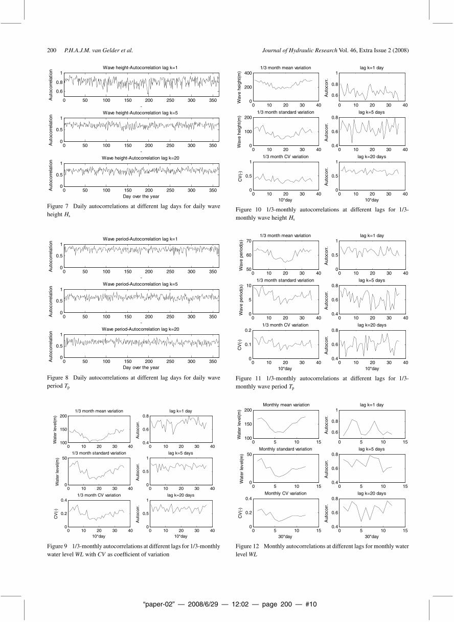
The result obtained with Eq. (42) is the autocorrelation func-tion on a day-by-day basis, referred to as the daily autocorrelationfunction here. It is calculated after detrending, log-transformingand de-seasonalizing the raw series. The daily autocorrelations atdifferent lags for the six daily coastal data processes are displayedin Figs 6–9. Similarly, the 1/3-monthly and monthly coastalseries can be de-seasonalized, to calculate their autocorrelationsat different lags for the six 1/3-monthly and monthly processes(Figs 10–14).

By a visual inspection of Figs 6 to 14, it can be concludedthat there are more or less seasonal variations in the autocorrela-tion structures of all the daily, the 1/3-monthly and the monthlycoastal data. In general, the autocorrelation is high for low-valueseasons and low for high-value seasons. However there are some

0 50 100 150 200 250 300 3500

0.5

1Water level-Autocorrelation lag k=1

-

Aut

ocor

rela

tion

0 50 100 150 200 250 300 3500

0.5


-

Aut

ocor

rela

tion

0 50 100 150 200 250 300 3500

0.5


Day over the year

Aut

ocor

rela

tion

Figure 6 Daily autocorrelations at different lag days for daily waterlevel WL

“paper-02” — 2008/6/29 — 12:02 — page 200 — #10


0 50 100 150 200 250 300 350

0.6

0.8

1Wave height-Autocorrelation lag k=1

-

Aut

ocor

rela

tion

0 50 100 150 200 250 300 3500

0.5


-

Aut

ocor

rela

tion

0 50 100 150 200 250 300 3500

0.5


Day over the year

Aut

ocor

rela

tion

Figure 7 Daily autocorrelations at different lag days for daily waveheight Hs

0 50 100 150 200 250 300 3500

0.5

1Wave period-Autocorrelation lag k=1

-

Aut

ocor

rela

tion

0 50 100 150 200 250 300 3500

0.5


-

Aut

ocor

rela

tion

0 50 100 150 200 250 300 3500

0.5


Day over the year

Aut

ocor

rela

tion

Figure 8 Daily autocorrelations at different lag days for daily waveperiod Tp

0 10 20 30 40100

150

2001/3 month mean variation

Wat

er le

vel(m

)

0 10 20 30 400

501/3 month standard variation

Wat

er le

vel(m

)

0 10 20 30 400

0.2

0.41/3 month CV variation

10*day

CV

(-)

0 10 20 30 400.4

0.6

0.8lag k=1 day

Aut

ocor

r.

0 10 20 30 400

0.5

1lag k=5 days

Aut

ocor

r.

0 10 20 30 400

0.5

1lag k=20 days

10*day

Aut

ocor

r.

Figure 9 1/3-monthly autocorrelations at different lags for 1/3-monthlywater level WL with CV as coefficient of variation

0 10 20 30 400

200


Wav

ehe

ight

(m)

0 10 20 30 400

100


Wav

e he

ight

(m)

0 10 20 30 400

0.5

11/3 month CV variation

10*day

CV

(-)

0 10 20 30 40

0.6

0.8

1lag k=1 day

Aut

ocor

r.

0 10 20 30 400.4

0.6

0.8lag k=5 days

Aut

ocor

r.

0 10 20 30 400

0.5

1lag k=20 days

10*day

Aut

ocor

r.

Figure 10 1/3-monthly autocorrelations at different lags for 1/3-monthly wave height Hs

0 10 20 30 4050

60


Wav

epe

riod(

s)

0 10 20 30 400

5


Wav

epe

riod(

s)

0 10 20 30 400

0.1

0.21/3 month CV variation

10*day

CV

(-)

0 10 20 30 400

0.5

1lag k=1 day

Aut

ocor

r.

0 10 20 30 400.4

0.6

0.8lag k=5 days

Aut

ocor

r.

0 10 20 30 400.4

0.6

0.8lag k=20 days

10*day

Aut

ocor

r.

Figure 11 1/3-monthly autocorrelations at different lags for 1/3-monthly wave period Tp

0 5 10 15100

150

200Monthly mean variation

Wat

er le

vel(m

)

0 5 10 150

50Monthly standard variation

Wat

er le

vel(m

)

0 5 10 150

0.2

0.4Monthly CV variation

30*day

CV

(-)

0 5 10 15

0.6

0.8

1lag k=1 day

Aut

ocor

r.

0 5 10 150.4

0.6

0.8lag k=5 days

Aut

ocor

r.

0 5 10 150.4

0.6

0.8lag k=20 days

30*day

Aut

ocor

r.

Figure 12 Monthly autocorrelations at different lags for monthly waterlevel WL

“paper-02” — 2008/6/29 — 12:02 — page 201 — #11


0 5 10 15200

300


Wav

ehe

igh

(m)

0 5 10 150

100


Wav

ehe

igh(

m)

0 5 10 150

0.2


30*day

CV

(-)

0 5 10 150.4

0.6

0.8lag k=1 day

Aut

ocor

r.

0 5 10 150.4

0.6

0.8lag k=5 days

Aut

ocor

r.

0 5 10 150.4

0.6

0.8lag k=20 days

30*day

Aut

ocor

r.

Figure 13 Monthly autocorrelations at different lags for monthly Hs

0 5 10 1560

70


Wav

epe

riod(

s)

0 5 10 150

5


Wav

epe

riod(

s)

0 5 10 150

0.1


30*day

CV

(-)

0 5 10 150.4

0.6

0.8lag k=1 day

Aut

ocor

r.

0 5 10 150

0.5

1lag k=5 days

Aut

ocor

r.

0 5 10 150

0.5

1lag k=20 days

30*day

Aut

ocor

r.

Figure 14 Monthly autocorrelations at different lags for monthly Tp

points where the autocorrelation are suddenly low. These could beconsidered as outliers. Daily autocorrelations of the water leveldata are generally higher than those for wave data. The dailyautocorrelations of daily coastal data are at about 0.6 to 0.9 forlag k = 1 having high variation properties. The daily autocorre-lations decrease as lag k increases. A similar trend is found forthe 1/3-monthly and the monthly coastal data series.

5 Long-memory analysis

5.1 Introduction to long-memory

Long-memory, or long-range dependence, refers to a non-negligible dependence between distant observations of a timeseries. Since the early work of Hurst (1951), it was well rec-ognized that many time series in diverse fields of application,such as financial time series (e.g., Lo, 1991; Lee and Schmidt,1996; Meade and Maier, 2003), meteorological time series (e.g.,Haslett and Raftery, 1989; Bloomfield, 1992; Hussain and Elber-gali, 1999) or internet traffic time series (e.g., Karagiannis et al.,

2004), may exhibit the phenomenon of long-memory or long-range dependence. In the hydrology community, studies werecarried out on the test for long-memory in streamflow pro-cesses. Montanari et al. (1997) applied a fractionally integratedautoregressive moving average (ARFIMA, see Appendix 3 fora brief description) model to the monthly and daily inflows ofLake Maggiore, Italy. Rao and Bhattacharya (1999) exploredsome monthly and annual hydrologic time series, including aver-age monthly streamflow, maximum monthly streamflow, averagemonthly temperature and monthly precipitation at various sta-tions in the mid-western United States. They stated that thereis little evidence of long-term memory in monthly hydrologicseries, and for annual series the evidence for lack of long-termmemory is inconclusive. Montanari et al. (2000) introduced a sea-sonal ARFIMA model and applied it to the Nile River monthlyflows at Aswan to detect whether long-memory is present. Theresulting model also indicates that non-seasonal long-memory isnot present in the data. At approximately the same time, Oomsand Franses (2001) documented that monthly river flow data dis-plays long-memory, in addition to pronounced seasonality basedon simple time series plots and periodic sample autocorrelations.

Long-memory processes can be expressed either in the time,or in the frequency domain. In the time domain, long-memoryis characterized by a hyperbolically decaying autocorrelationfunction. It decays so slowly that the autocorrelations are notassumable. For a stationary discrete long-memory time seriesprocess, its autocorrelation function ρ(k) at lag k satisfies(Hosking, 1981)

ρ(k) : �(1 − d)

�(d)k2d−1, as k → ∞, (45)

where d is the long-memory parameter or the fractional differ-encing parameter, and 0 < |d| < 0.5.

In the frequency domain, the long-memory manifests itself asan unbounded spectral density at zero frequency. For a stationarydiscrete long-memory time series process, its spectral density atzero frequency satisfies

f(λ) ∼ Cλ1−2H, as λ → 0+,for a positive, finite C. H is called the Hurst coefficient or theself-similarity parameter, as originally defined by Hurst (1951),representing the classical parameter characterizing long-memory.H is related to the fractional differencing parameter d as d =H − 0.5.

A number of models were proposed to describe the long-memory feature of time series. The Fractional Gaussian Noisemodel was the first with long-range dependence introducedby Mandelbrot and Wallis (1969). Then, Hosking (1981) andGranger and Joyeux (1980) proposed the fractional integratedautoregressive and moving average model, denoted by ARFIMA(p, d, q). When −0.5 < d < +0.5, the ARFIMA (p, d, q)process is stationary, and if 0 < d < 0.5 the process presentslong-memory behavior.

Many methods are available for testing the existence of long-memory and estimating the Hurst coefficient H or the fractionaldifferencing parameter d. Many of them are well described by

“paper-02” — 2008/6/29 — 12:02 — page 202 — #12


Beran (1994). These techniques include graphical methods (e.g.,the classical R/S analysis; or the aggregated variance method),parametric methods (e.g., Whittle maximum likelihood estima-tion method) and semi-parametric methods (e.g., GPH methodand local whittle method). Heuristic methods are useful to testif a long-range dependence exists in the data and to find a firstestimate of d or H , but they are generally neither accurate norrobust. The parametric methods obtain consistent estimators ofd or H via a maximum likelihood estimation (MLE) of para-metric long-memory models. They give more accurate estimatesof d or H , but generally require knowledge of the true modelwhich is in fact always unknown. The semi-parametric meth-ods, such as the GPH method (Geweke and Porter-Hudak, 1983),seek to estimate d under few prior assumptions concerning thespectral density of a time series and, in particular, without spec-ifying a finite parameter model for the dth difference of the timeseries. Herein, the statistic GPH test which is a semi-parametricmethod will be used to test for the null hypothesis of no presenceof long-memory. Besides, an approximate maximum likelihoodestimation method is used to estimate the fractional differencingparameter d, but without testing for the significance level of theestimation.

Two heuristic methods will be used below, namely the autocor-relation function analysis, and the aggregated variance methodto detect the existence of long-memory in the coastal processesat Noordwijk location. Then, the GPH test (Geweke and Porter-Hudak, 1983) is used to test for the existence of long-memoryin the coastal processes of all the five rivers, and the maximumlikelihood estimates of the fractional differencing parameter dwill be made as well.

5.2 Detecting long-memory with heuristic methods

5.2.1 Autocorrelation function analysisIn the presence of long-memory, the autocorrelation function(ACF) of a time series decreases to 0 at a much slower rate thanthe exponential rate implied by a short-memory ARMA model.The sample ACF of the observed time series under investigationcan then be compared with the theoretical ACF (McLeod, 1975)of theARMA model fitted to the time series. If the sampleACF ofthe observed series decays much slower than theACF of the fittedARMA model, then the existence of long-memory is indicated.

0

-0.2

0.0

0.2ac

fAR

0.4

0.6

0.8

1.0

20 40

Lag k(a)-Water level

60 80 100 0

0.0

0.2

acfA

R

0.4

0.6

0.8

1.0

20 40

Lag k(b)-Wave height

60 80 100 0

0.0

0.2

acfA

R

0.4

0.6

0.8

1.0

20 40

Lag k(c)-Wave period

60 80 100

Figure 15 Theoretical ACF daily coastal data

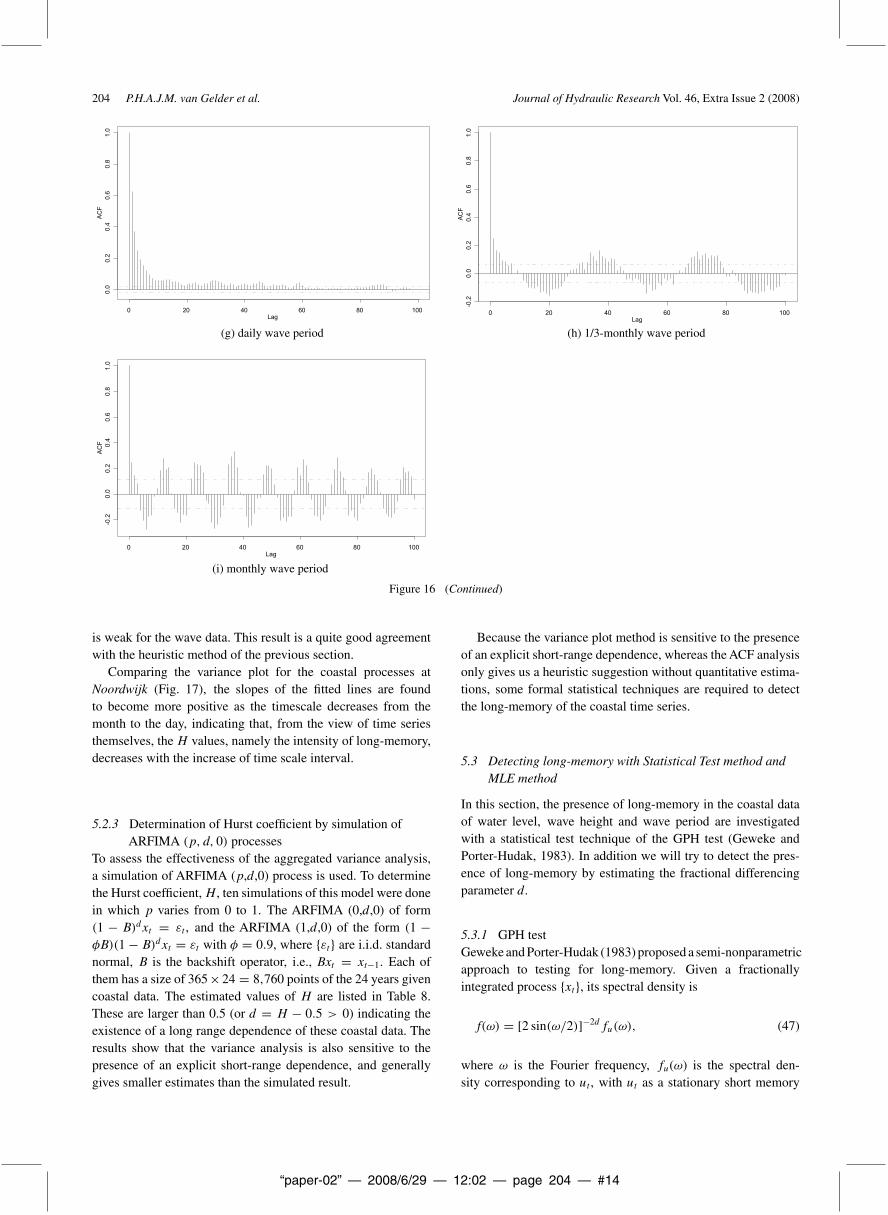
The theoretical ACF are plotted in Fig. 15. The sample ACFof the coastal time series of the fitted models from lag 1 to lag100 are plotted in Figs 16–18. The autocorrelation estimate ateach lag is given by the height of the vertical lines. The valueof the autocorrelation function at lag 0 is always 1. The horizon-tal band about zero represents the approximate 95% confidencelimits forH0 ≈ 0. If no autocorrelation estimate falls outside thestrip defined by the two dotted lines, and the data contain no out-liers, it may be safely assumed that there is no serial correlation.Otherwise, there should be concern about the presence of a serialcorrelation. Then, the ACF plot indicates serial correlation fromlags 1 to 8 of daily and 1/3-monthly water levels, 1 to 4 lags ofmonthly water level data. The long range correlation increasesfor the dailyHs and the daily Tp data up to lags 64. It decreases forthose of the 1/3-monthly and the monthly data by similar trend.

Upon comparing the theoretical ACF of the fitted AR modelswith the sample ACF of the observed coastal series, one findthat:

(1) The daily coastal time series is highly persistent and the auto-correlation remains significant from zero at lag 100. Thetheoretical autocorrelation closely matches the sample auto-correlation at short lags from lag 1 to lag 10. However, forlarge lags, the sample ACF decays much slower than thetheoretical ACF.

(2) The 1/3-monthly and monthly coastal time series are muchless persistent. For both 1/3-monthly coastal series of waterlevels, significant wave heights and wave periods, the sam-ple autocorrelations are slightly larger than the theoreticalautocorrelations for large lags.

5.2.2 Aggregated Variance Method (AVM)For independent random variables x1, . . . , xN , the variance ofsample mean is equal to Var(x) = σ2N−1. In presence of long-memory, Beran (1994) proved that the variance of the samplemean may be expressed by var(x) ≈ cN2H−2, where c > 0.Correspondingly, Beran suggested the following method forestimating the Hurst coefficient H :

(1) Take a sufficient number (say m) of sub-series of lengthk (2 ≤ k ≤ N/2), calculate the sample meansx1(k), x2(k), . . . , xm(k) and the overall mean x(k) =m−1∑m

j=1 xj(k);

“paper-02” — 2008/6/29 — 12:02 — page 203 — #13


(2) For each k, calculate the sample variance s2(k) of the msample means using

s2(k) = (k − 1)−1k∑j=1

(xj(k)− x(k))2 (46)

(3) Plot log[s2(k)] against log k. For large values of k, the pointsin this plot are expected to be scattered around a straightline with a negative slope (2H − 2). The slope is steeper

Lag

ACF

0 20 40 60 80 100

0.0

0.2

0.4

0.6

0.8

1.0

Lag

ACF

0 20 40 60 80 100

-0.2

0.0

0.2

0.4

0.6

0.8

1.0

(a) Daily water level (b) 1/3-monthly water level

Lag

ACF

0 20 40 60 80 100

-0.4

-0.2

0.0

0.2

0.4

0.6

0.8

1.0

Lag

ACF

0 20 40 60 80 100

0.0

0.2

0.4

0.6

0.8

1.0

(c) monthly water level (d) daily wave height

Lag

ACF

0 20 40 60 80 100

-0.2

0.0

0.2

0.4

0.6

0.8

1.0

Lag

ACF

0 20 40 60 80 100

-0.4

-0.2

0.0

0.2

0.4

0.6

0.8

1.0

(e) 1/3-monthly wave height (f) monthly wave height

Figure 16 Sample ACF (vertical lines) for daily, 1/3-monthly and monthly coastal data at Noordwijk

(more negative) for short-memory processes. In the case ofindependence, the ultimate slope is −1.

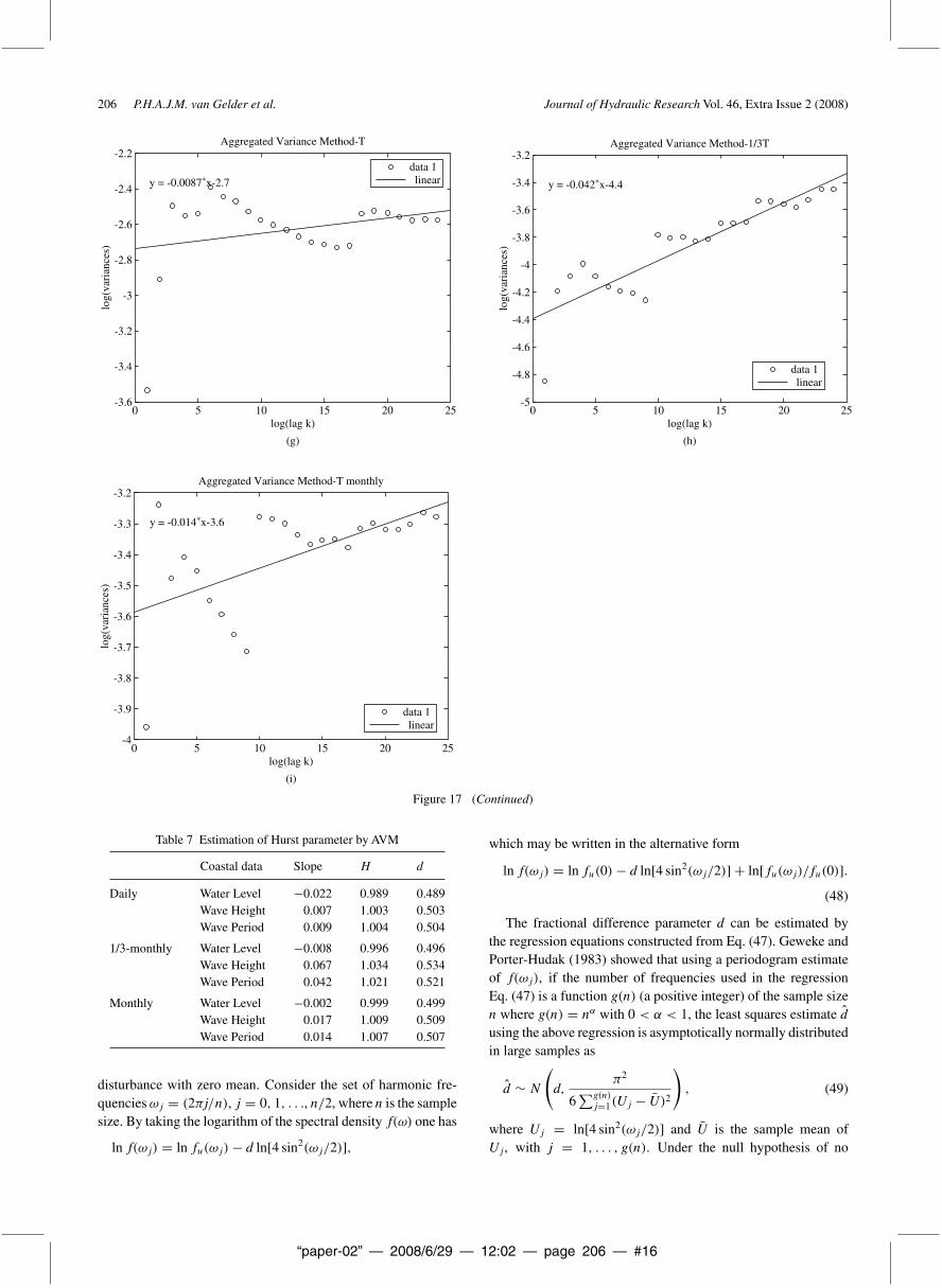
The variance analysis for the coastal data at Noordwijk is givenin Fig. 17. The Hurst coefficient and the d value are summarizedin Table 7. According to this method the long range dependenceexists clearly in the water level data at all time scale intervals(daily, 1/3-monthly and monthly). The intensity of dependencedecreases as the time scale interval is increased. The dependence

“paper-02” — 2008/6/29 — 12:02 — page 204 — #14


Lag

ACF

0 20 40 60 80 100

0.0

0.2

0.4

0.6

0.8

1.0

Lag

ACF

0 20 40 60 80 100

-0.2

0.0

0.2

0.4

0.6

0.8

1.0

(g) daily wave period (h) 1/3-monthly wave period

Lag

ACF

0 20 40 60 80 100

-0.2

0.0

0.2

0.4

0.6

0.8

1.0

(i) monthly wave period

Figure 16 (Continued)

is weak for the wave data. This result is a quite good agreementwith the heuristic method of the previous section.

Comparing the variance plot for the coastal processes atNoordwijk (Fig. 17), the slopes of the fitted lines are foundto become more positive as the timescale decreases from themonth to the day, indicating that, from the view of time seriesthemselves, the H values, namely the intensity of long-memory,decreases with the increase of time scale interval.

5.2.3 Determination of Hurst coefficient by simulation ofARFIMA (p, d, 0) processes

To assess the effectiveness of the aggregated variance analysis,a simulation of ARFIMA (p,d,0) process is used. To determinethe Hurst coefficient,H , ten simulations of this model were donein which p varies from 0 to 1. The ARFIMA (0,d,0) of form(1 − B)dxt = εt , and the ARFIMA (1,d,0) of the form (1 −φB)(1 − B)dxt = εt with φ = 0.9, where {εt} are i.i.d. standardnormal, B is the backshift operator, i.e., Bxt = xt−1. Each ofthem has a size of 365 × 24 = 8,760 points of the 24 years givencoastal data. The estimated values of H are listed in Table 8.These are larger than 0.5 (or d = H − 0.5 > 0) indicating theexistence of a long range dependence of these coastal data. Theresults show that the variance analysis is also sensitive to thepresence of an explicit short-range dependence, and generallygives smaller estimates than the simulated result.

Because the variance plot method is sensitive to the presenceof an explicit short-range dependence, whereas the ACF analysisonly gives us a heuristic suggestion without quantitative estima-tions, some formal statistical techniques are required to detectthe long-memory of the coastal time series.

5.3 Detecting long-memory with Statistical Test method andMLE method

In this section, the presence of long-memory in the coastal dataof water level, wave height and wave period are investigatedwith a statistical test technique of the GPH test (Geweke andPorter-Hudak, 1983). In addition we will try to detect the pres-ence of long-memory by estimating the fractional differencingparameter d.

5.3.1 GPH testGeweke and Porter-Hudak (1983) proposed a semi-nonparametricapproach to testing for long-memory. Given a fractionallyintegrated process {xt}, its spectral density is

f(ω) = [2 sin(ω/2)]−2dfu(ω), (47)

where ω is the Fourier frequency, fu(ω) is the spectral den-sity corresponding to ut , with ut as a stationary short memory

“paper-02” — 2008/6/29 — 12:02 — page 205 — #15


0-0.9

-0.8

-0.7

-0.6

-0.5

-0.4

-0.3

-0.2

-0.1

0

y = -0.022∗x-0.29

Aggregated Variance Method-Daily WL

data 1linear

5 10log(lag k)

log(

vari

ance

s)

15 20 25 0-1.4

-1.3

-1.2

-1.1

-1

-0.9

-0.8

-0.7

-0.6

y = -0.0084∗x-1

Aggregated Variance Method-1/3month WL

data 1linear

5 10log(lag k)

(a) (b)

log(

vari

ance

s)

15 20 25

0-1.4

-1.3

-1.2

-1.1

-1

-0.9

-0.8

-0.7

-0.6

-0.5

y = -0.0021∗x-0.96

Aggregated Variance Method-monthly WL

data 1linear

5 10log(lag k)

log(

vari

ance

s)

15 20 25 0-1.8

-1.6

-1.4

-1.2

-1

-0.8

-0.6

-0.4

-0.2

0

y = -0.0068∗x-0.58

Aggregated Variance Method-Hs

data 1linear

5 10log(lag k)

(c) (d)

log(

vari

ance

s)

15 20 25

0-5

-4.5

-4

-3.5

-3

-2.5

-2

-1.5

-1

-0.5

y = -0.067∗x-2.7

Aggregated Variance Method-1/3Hs

5 10log(lag k)

log(

vari

ance

s)

15 20 25 0-1.8

-1.7

-1.6

-1.5

-1.4

-1.3

-1.2

-1.1

y = -0.017∗x-1.6

Aggregated Variance Method-Hs monthly

data 1linear

5 10log(lag k)

(e) (f)

log(

vari

ance

s)

15 20 25

data 1linear

Figure 17 (a–i) Variance analyses to see long range dependence of daily, 1/3-monthly and monthly coastal data at Noordwijk location

“paper-02” — 2008/6/29 — 12:02 — page 206 — #16


0-3.6

-3.4

-3.2

-3

-2.8

-2.6

-2.4

-2.2

y = -0.0087∗x-2.7

Aggregated Variance Method-T

data 1linear

5 10log(lag k)

log(

vari

ance

s)

15 20 25

(g)

0-5

-4.8

-4.6

-4

-4.2

-4.4

-3.8

-3.6

-3.4

-3.2

y = -0.042∗x-4.4

Aggregated Variance Method-1/3T

data 1linear

5 10log(lag k)

log(

vari

ance

s)

15 20 25

(h)

0-4

-3.9

-3.6

-3.7

-3.8

-3.5

-3.4

-3.3

-3.2

y = -0.014∗x-3.6

Aggregated Variance Method-T monthly

data 1linear

5 10log(lag k)

log(

vari

ance

s)

15 20 25

(i)

Figure 17 (Continued)

Table 7 Estimation of Hurst parameter by AVM

Coastal data Slope H d

Daily Water Level −0.022 0.989 0.489Wave Height 0.007 1.003 0.503Wave Period 0.009 1.004 0.504

1/3-monthly Water Level −0.008 0.996 0.496Wave Height 0.067 1.034 0.534Wave Period 0.042 1.021 0.521

Monthly Water Level −0.002 0.999 0.499Wave Height 0.017 1.009 0.509Wave Period 0.014 1.007 0.507

disturbance with zero mean. Consider the set of harmonic fre-quenciesωj = (2πj/n), j = 0, 1, . . ., n/2, where n is the samplesize. By taking the logarithm of the spectral density f(ω) one has

ln f(ωj) = ln fu(ωj)− d ln[4 sin2(ωj/2)],

which may be written in the alternative form

ln f(ωj) = ln fu(0)− d ln[4 sin2(ωj/2)] + ln[fu(ωj)/fu(0)].(48)

The fractional difference parameter d can be estimated bythe regression equations constructed from Eq. (47). Geweke andPorter-Hudak (1983) showed that using a periodogram estimateof f(ωj), if the number of frequencies used in the regressionEq. (47) is a function g(n) (a positive integer) of the sample sizen where g(n) = nα with 0 < α < 1, the least squares estimate dusing the above regression is asymptotically normally distributedin large samples as

d ∼ N

(d,

π2

6∑g(n)

j=1(Uj − U)2

), (49)

where Uj = ln[4 sin2(ωj/2)] and U is the sample mean ofUj , with j = 1, . . . , g(n). Under the null hypothesis of no

“paper-02” — 2008/6/29 — 12:02 — page 207 — #17


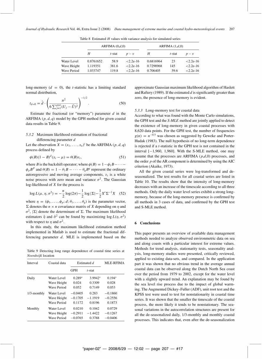
Table 8 Estimated H values with variance analysis for simulated series

ARFIMA (0,d,0) ARFIMA (1,d,0)

H t-stat p− v H t-stat p− v

Water Level 0.8761652 58.9 <2.2e-16 0.6816964 23 <2.2e-16Wave Height 1.119351 381.6 <2.2e-16 0.7298968 145 <2.2e-16Wave Period 1.033747 119.8 <2.2e-16 0.706405 59.6 <2.2e-16

long-memory (d = 0), the t-statistic has a limiting standardnormal distribution,

td=0 = d ·(

π2

6∑g(n)

j=1(Uj − U)2

)−1/2

. (50)

Estimate the fractional (or “memory”) parameter d in theARFIMA (p, d, q) model by the GPH method for given coastaldata results in Table 9.

5.3.2 Maximum likelihood estimation of fractionaldifferencing parameter d

Let the observation X = (x1, . . . , xn)t be the ARFIMA (p, d, q)

process defined by

φ(B)(1 − B)d(xt − µ) = θ(B)εt, (51)

whereB is the backshift operator; where φ(B) = 1−φ1B−· · ·−φpB

P and θ(B) = 1 − θ1B − · · · − θqBq represent the ordinary

autoregressive and moving average components, εt is a whitenoise process with zero mean and variance σ2. The Gaussianlog-likelihood of X for the process is

logL(µ, η, σ2) = −n2

log(2π)− 1

2log |�|− 1

2Xt�−1X (52)

where η = (φ1, . . . , φp; d; θ1, . . . , θq) is the parameter vector,� denotes the n× n covariance matrix of X depending on η andσ2, |�| denote the determinant of �. The maximum likelihoodestimators η and σ2 can be found by maximizing logL(η, σ2)

with respect to η and σ2.In this study, the maximum likelihood estimation method

implemented in Matlab is used to estimate the fractional dif-ferencing parameter d. MLE is implemented based on the

Table 9 Detecting long range dependence of coastal time series atNoordwijk location

Interval Coastal data Estimated d MLE-RFIMA

GPH t-stat

Daily Water Level 0.289∗ 3.9942∗ 0.194∗

Wave Height 0.024 0.3309 0.028Wave Period 0.052 0.7149 0.053

1/3-monthly Water Level −0.0405 0.283 −0.1860Wave Height −0.1705 −1.1919 −0.2556Wave Period 0.1172 0.8196 0.1873

Monthly Water Level 0.0210 0.1042 0.0729Wave Height −0.2911 −1.4422 −0.1267Wave Period −0.0765 0.3788 −0.0406

approximate Gaussian maximum likelihood algorithm of Haslettand Raftery (1989). If the estimated d is significantly greater thanzero, the presence of long-memory is evident.

5.3.3 Long-memory test for coastal dataAccording to what was found with the Monte Carlo simulations,the GPH test and the S-MLE method are jointly applied to detectthe existence of long-memory in given coastal processes with8,620 data points. For the GPH test, the number of frequenciesg(n) = n−0.5 was chosen as suggested by Geweke and Porter-Hudak (1983). The null hypothesis of no long-term dependenceis rejected if a t-statistic in the GPH test is not contained in theinterval [−1,960, 1,960]. With the S-MLE method, one mayassume that the processes are ARFIMA (p,d,0) processes, andthe order p of the AR component is determined by using the AICcriterion (Akaike, 1973).

All the given coastal series were log-transformed and de-seasonalized. The test results for all coastal series are listed inTable 10. The results show that the intensity of long-memorydecreases with an increase of the timescale according to all threemethods. Only the daily water level series exhibit a strong long-memory, because of the long-memory presence is confirmed byall methods in 3 cases of data, and confirmed by the GPH testand S-MLE method.

6 Conclusions

This paper presents an overview of available data managementmethods needed to analyze observed environmetric data on seaand along coasts with a particular interest for extreme values.Methods for trend analysis, stationarity tests, seasonality anal-ysis, long-memory studies were presented, critically reviewed,applied to existing data-sets, and compared. In the applicationpart it was shown that no obvious trend in the average annualcoastal data can be observed along the Dutch North Sea coastover the period from 1979 to 2002, except for the water levelwith a slightly upward trend. An explanation may be found bythe sea level rise process due to the impact of global warm-ing. The Augmented Dickey–Fuller (ADF), unit root test and theKPSS test were used to test for nonstationarity in coastal timeseries. It was shown that the smaller the timescale of the coastalprocess, the more likely it tends to be nonstationary. The sea-sonal variations in the autocorrelation structures are present forall the de-seasonalized daily, 1/3-monthly and monthly coastalprocesses. This indicates that, even after the de-seasonalization

“paper-02” — 2008/6/29 — 12:02 — page 208 — #18


procedure, the seasonality is still present, not in the mean andvariance, but in the autocorrelation structure.

The investigation of the long-memory phenomenon of coastalprocesses at different timescales shows that, with the increase oftimescale, the intensity of long-memory decreases. According tothe GPH test and the maximum likelihood estimation method,all daily coastal series are more or less considered as long rangedependent. However, only the daily water level series exhibit astrong long-memory. The presence of long-memory is satisfiedby all indicated tests. Comparing the stationary test results and thelong-memory test results, these two types of tests are more or lesslinked, not only in that the test results have similar timescale pat-terns, but also in that there is a general tendency that the strongerthe nonstationarity, the more intense the long-memory. Thereare some attempts to use the KPSS stationary tests to test for theexistence of long-memory. It is worthwhile to continue the inves-tigation on the issue of the relationship between nonstationarityand the long-memory.

Acknowledgements

The work described in this publication was supported by the Euro-pean Community’s Sixth Framework Programme through thegrant to the budget of the Integrated Project FLOODsite, ContractGOCE-CT-2004-505420. The paper reflects the authors’ viewsand not those of the European Community. Neither the EuropeanCommunity nor any member of the FLOODsite Consortium isliable for any use of the information in this paper.

Appendix 1 Stationarity and Periodic Stationarity

Let {xt}, t = 1, . . . , N be N consecutive observations of a sea-sonal time series with seasonal period s. For simplicity, assumethat N/s = n is an integer. In other words, there are n full yearsof data available. The time index parameter t may be writtent = t(r − m) = (r − 1)s + m, where r = 1, . . . , n and m =1, . . . , s. For monthly data s = 12 and r and m denote the yearand month. If µm = E(zt(r,m)) and γl,m = cov(zt(r,m), zt(r,m)−l)exist and depend only on l and m, zt is said to be periodicallycorrelated or periodic stationary (Gladysev, 1961). Note that thecase whereµm and γt,m do not depend onm reduces to an ordinarycovariance stationary time series.

A series {xt} is called stationary if, loosely speaking, its sta-tistical properties do not change with time. More precisely, {xt}is said to be completely stationary if, for any integer k, the jointprobability distribution of xt, xt+1, . . . , xt+k−1 is independent onthe time index t (e.g., Priestley, 1988).

Appendix 2 Brief description of ARMA-type Model

One of the most important and highly popularized time seriesmodels is theARMA-type model, includingAR,ARMA,ARIMAand seasonal ARIMA model, introduced by Box and Jenkins(1976). It has a long history of being applied to streamflowforecasting problems. For instance, McKerchar and Delleur

(1974) used an ARMA process to achieve stochastic modelingof monthly flows. McLeod et al. (1977) applied the ARMAapproach to average annual streamflows. Three types of seasonaltime series models are commonly used to model hydrologi-cal processes which usually have strong seasonality (Hipel andMcLeod, 1994): (1) Seasonal autoregressive integrated movingaverage (SARIMA) models, (2) De-seasonalizedARMA models,and (3) Periodic ARMA models. The de-seasonalized modelingapproach was adopted in this study. The general form of ARIMA(p,d,q) model is given by

φ(B)∇dxt = θ(B)εt, (53)

where B is the backshift operator, i.e., Bxt = xt−1; φ(B) =1−φ1B−· · ·−φpBP , and θ(B) = 1−θ1B−· · ·−θqBq representthe ordinary autoregressive and moving average components; εt isa white noise process with zero mean and variance σ2. ∇ = 1−Bis the first-order difference operator and ∇d = (1 − B)d is thed-fold differencing. When d = 0, the ARIMA (p,d,q) modelreduces to the ARMA (p,q) model

φ(B)xt = θ(B)εt

When q = 0, then the ARMA (p,q) model further reduces to theAR(p) model.

Box and Jenkins (1976) give the following paradigm for fittingARIMA models:

(1) Model identification: Determination of the ARIMA modelorders,

(2) Estimation of model parameters: The unknown parametersin Eq. (52) are estimated, and

(3) Diagnostics and model criticism: The residuals are used tovalidate the model and suggest potential alternative models,which may be better.

These steps are repeated until a satisfactory model is found.

Appendix 3 Brief description of ARFIMA Model

The general form of the ARFIMA (p,d,q) model is

φ(B)∇dxt = θ(B)εt, |d| < 0.5,

where φ(B), θ(B) and ∇d are identical as in Eq. (3.1). The dif-ference operator ∇d = (1 − B)d is by means of the binomialexpansion

∇d = (1 − B)d =∞∑j=0

πjBj

where

πj = �(j − d)

�(j + 1)�(−d) =∏

0≤k≤j

k − 1 − d

k, j = 0, 1, 2, . . .

The parameters φ, θ and d of the ARFIMA model may be esti-mated by the maximum likelihood method or log-periodogrambased regression method (e.g., Brockwell and Davis, 1991).The S-Plus function arima.fracdiff fits the ARFIMA models tounivariate time series data through approximate the Gaussianmaximum likelihood algorithm of Haslett and Raftery (1989).

“paper-02” — 2008/6/29 — 12:02 — page 209 — #19


Notation

ω = Fourier frequencyτ = Trend test statisticσ = Standard deviationχ = Test statistic for heterogeneity� = Gamma functionρ = Autocorrelation coefficientH = Hurst coefficientHs = Significant wave heightk = Time lag (day)N = Number of observation years

p, d, q = Parameters of ARIMA, ARFIMA modelsR = Matrix of ranks of random variablesS = Mann-Kendall test statistict = Test statistic of t-testTp = Wave peak periodxi = Random variable iβt = Deterministic trendεt = Stationary error

References

Akaike, H. (1973). “Information Theory and an Extension ofthe Maximum Likelihood Principle”. Proc. 2nd Intl. Symp.Information Theory, B.N. Petrov, F. Csaki (eds.), pp. 267–281,Akademia Kiado, Budapest.

Bartlett, M.S. (1950). “Periodogram Analysis and ContinuousSpectra”. Biometrika 37, 1–16.

Beran, J. (1994). “Statistics for Long-Memory Processes”.Chapman & Hall, New York.

Bloomfield, P. (1992). “Trend in Global Temperature”. ClimaticChange 21, 1–16.

Box, G.E.P., Cox, D.R. (1964). “An Analysis of Transforma-tions”. J. Royal Statistical Society, Ser. B, 26, 211–252.

Box, G.E.P., Jenkins, G.M. (1976). “Time Series Analysis: Fore-casting and Control”, 2nd (edn.) Holden-Day, San Francisco.

Burn, D.H., Hag Elnur, M.A. (2002). “Detection of HydrologicalTrend and Variability”. J. Hydrol. 255, 107–122.

Chen, H.L., Rao, A.R. (2002). “Testing Hydrological Time Seriesfor Stationarity”. J. Hydrol. Eng. 7(2), 129–136.

Dickey, D.A., Fuller, W.A. (1979). “Distribution of the Estima-tors for Autoregressive Time Series with a Unit Root”. J. Am.Stat. Assoc. 74, 423–431.

Dietz, E.J., Killeen, T.J. (1981). “A Nonparametric MultivariateTest for Monotonic Trend with Pharmaceutical Applications”.J. Am. Stat. Assoc. 76(373), 169–174.

Douglas, E.M., Vogel, R.M., Kroll, C.N. (2000). “Trends inFloods and Low Flows in the United States: Impact of SpatialCorrelation”. J. Hydrol. 240, 90–105.

Fuller, W.A. (1976). “Introduction to statistical time series”.Wiley, New York.

Geweke, J., Porter-Hudak, S. (1983). “The Estimation andAppli-cation of Long Memory Time Series Models”. J. Time Ser.Anal. 4, 221–238.

Gimeno, R., Manchado, B., Minguez, R. (1999). “StationarityTests for Financial Time Series”. Physica A 269, 72–78.

Gladysev, E.G. (1961). “Periodically Correlated RandomSequences”. Soviet Math. Dokl. 2, 385–388.

Granger, C.W.J., Joyeux, R. (1980). “An Introduction to Long-Memory Time Series Models and Fractional Differencing”.J. Time Ser. Anal. 1, 15–29.

Hamilton, J.D. (1994). “Time Series Analysis”. PrincetonUniversity Press, Princeton.

Haslett, J., Raftery, A.E. (1989). “Space-Time Modelingwith Long-Memory Dependence: Assessing Ireland’s WindPower Resource” (with Discussion). Applied Statistics 38,1–50.

Helsel, D.R., Hirsch, R.M. (1992). “Statistical Methods in WaterResources”. Elsevier, Amsterdam.

Hirsch, R.M., Slack, J.R. (1984). “A Nonparametric Trend Testfor Seasonal Data with Serial Dependence”. Water ResourcesResearch 20(6), 727–732.

Hirsch, R.M., Slack, J.R., Smith, R.A. (1982). “Techniquesof Trend Analysis for Monthly Water Quality Data”. WaterResources Research 18(1), 107–121.

Hosking, J.R.M. (1981). “Fractional Differencing”. Biometrika68, 165–176.

Hurst, H.E. (1951). “Long-Term Storage Capacity of Reser-voirs”. Trans. ASCE 116, 770–808.

Hussain, S., Elbergali, A. (1999). “Fractional Order Estima-tion and Testing, Application to Swedish Temperature Data”.Environmetrics 10, 339–349.

Insightful Corporation (2001). “Analyzing Time Series and Sig-nals, of the S-PLUS 6 for Windows Guide to Statistics”, Vol. 2,Chap. 27, Insightful Corporation, Seattle WA.

Jain, S., Lall, U. (2001). “Floods in a Changing Climate: Doesthe Past Represent the Future”? Water Res. Research 37(12),3193–3205.

Karagiannis, T., Molle, M., Faloutsos, M. (2004). “Long-RangeDependence: Ten Years of Internet Traffic Modeling”. IEEEInternet Computing 8(5), 57–64.

Kendall, M.G. (1938). “A New Measure of Rank Correlation”.Biometrika 30, 81–93.

Kendall, M.G. (1975). “Rank Correlation Methods”. Griffin,London.

Kundzewicz, Z.W., Graczyk, D., Maurer, T., Przymusinska, I.,Radziejewski, M., Svensson, C., Szwed, M. (2004). “Detec-tion of Change in World-Wide Hydrological Time Series ofMaximum Annual Flow”. GRDC Report 32. Global RunoffData Centre, Koblenz, Germany.

Kwiatkowski, D., Phillips, P.C.B., Schmidt, P., Shin, Y. (1992).“Testing the Null of Stationarity Against the Alternative of aUnit Root: How Sure are We that Economic Time Series Havea Unit Root”? J. Econometrics 54, 159–178.

Lee, D., Schmidt, P. (1996). “On the Power of the KPSS Testof Stationarity Against Fractionally-Integrated Alternatives”.J. Econometrics 73(1), 285–302.

Lettenmaier, D.P., Wood, E.F. (1993). “Hydrological Forecast-ing, Handbook of Hydrology”, Chap. 26, D.R. Maidment,(ed.) McGraw-Hill, New York.

“paper-02” — 2008/6/29 — 12:02 — page 210 — #20


Lo, A.L. (1991). “Long-Term Memory in Stock Market Prices”.Econometrica 59(5), 1279–1313.

Mandelbrot, B.B., Wallis, J.R. (1969a). “Computer Experimentswith Fractional Gaussian Noises”. Water Res. Research 5,228–267.

Mandelbrot, B.B., Wallis, J.R. (1969b). “Robustness of theRescaled Range R/S in the Measurement of Non-CyclicLong-Run Statistical Dependence”. Water Res. Research 5,967–988.

Mann, H.B. (1945). “Nonparametric TestAgainst Trend”. Econo-metrica 13, 245–259.

McLeod, A.I. (1975). “Derivation of the Theoretical Autoco-variance Function of Autoregressive-Moving Average TimeSeries”. Applied Statistics 24(2), 255–256.

Meade, N., Maier, M.R. (2003). “Evidence of Long Memory inShort-Term Interest Rates”. J. Forecast. 22, 553–568.

Mitosek, H.T. (2000). “On Stochastic Properties of Daily RiverFlow Processes”. J. Hydrol. 228, 188–205.

Montanari, A., Rosso, R., Taqqu, M.S. (1997). “FractionallyDifferenced ARIMA Models Applied to Hydrological TimeSeries: Identification, Estimation, and Simulation”. Water Res.Research 33(5), 1035–1044.

Montanari, A., Rosso, R., Taqqu, M.S. (2000). “A Seasonal Frac-tional ARIMA Model Applied to the Nile River Monthly atAswan”. Water Res. Research 36, 1249–1259.

Newey, W.K., West, K.D. (1987). “A Simple, Positive Semi-Definite, Heteroskedasticity and Autocorrelation ConsistentCovariance Matrix”. Econometrica 55, 703–708.

Ooms, M., Franses, P.H. (2001). “A Seasonal Periodic LongMemory Model for Monthly River Flows”. EnvironmentalModelling and Software 16, 559–569.

Priestley, M.B. (1988). “Non-Linear and Non-Stationary TimeSeries Analysis”. Academic Press, London.

Rao, A.R., Bhattacharya, D. (1999). “Hypothesis Testing forLong-Term Memory in Hydrological Series”. J. Hydrol.216(3/4), 183–196.

Said, S.E., Dickey, D. (1984). “Testing for Unit Roots in Autore-gressive Moving-Average Models with Unknown Order”.Biometrika 71, 599–607.

Schwert, G.W. (1989). “Tests for Unit Roots: A Monte CarloInvestigation”. J. Business Eco. Stat. 7, 147–159.

Shin, Y., Schmidt, P. (1992). “The KPSS Stationarity Test as aUnit Root Test”. Economics Letters 38, 387–392.

van Belle, G., Hughes, J.P. (1984). “Nonparametric Testsfor Trend in Water Quality”. Water Res. Research 20(1),127–136.

van Gelder, P.H.A.J.M. (1999). “Statistical Methods for the Risk-Based Design of Civil Structures”. Communication 00-1 onHydraulic and Geotechnical Engineering, ISSN: 0169-6548,TU Delft, The Netherlands.

von Storch, H. (1995). “Misuses of StatisticalAnalysis in ClimateResearch. Analysis of ClimateVariability: Applications of Sta-tistical Techniques”, H.V. Storch, A. Navarra (eds.), pp. 11–26,Springer, New York.

Wang, W. (2006). “Stochasticity, Nonlinearity and Forecasting ofStreamflow Processes”. PhD thesis. University of Technology,Delft.

Zhang, X., Harvey, K.D., Hogg, W.D., Yuzyk, T.R. (2001).“Trends in Canadian Streamflow”. Water Res. Research 37(4),987–998.

Zivot, E., Wang, J. (2002). “Modelling Financial Time Serieswith S-Plus”. Springer, New York.

data management of extreme marine and coastal hydro ... faculteit/afdelingen... · ghahfaroki...

Documents