data-driven network analysis and applications
TRANSCRIPT

Data Driven NetworkAnalysis and Applications
Dissertation
zur Erlangung des DoktorgradesDr. rer. nat.
der Mathematisch-Naturwissenschaftlichen Fakultatender Georg-August-Universitat zu Gottingen
im PhD Programme in Computer Science (PCS)der Georg-August University School of Science (GAUSS)
vorgelegt von
Narisu Taoaus Inner Mongolia, China
Gottingenim August 2015

Betreuungsausschuss: Prof. Dr. Xiaoming Fu,Georg-August-Universitat Gottingen
Dr. Jan Nagler,Eidgenossische Technische Hochschule Zurich
Prufungskommission:Referent: Prof. Dr. Xiaoming Fu,
Georg-August-Universitat Gottingen
Korreferenten: Prof. Dr. Dieter Hogrefe,Georg-August-Universitat Gottingen
Weitere Mitglieder Prof. Dr. K.K. Ramakrishnan,der Prufungskommission: University of California, Riverside, USA
Prof. Dr. Carsten Damm,Georg-August-Universitat Gottingen
Prof. Dr. Winfried Kurth,Georg-August-Universitat Gottingen
Prof. Dr. Burkhard Morgenstern,Georg-August-Universitat Gottingen
Tag der mundlichen Prufung: 14. September 2015

Abstract
Data is critical for scientific research and engineering systems. However, data collectionprocedures are often subject to high cost or heavy loss rate. It is challenging to accuratelyestimate missing or unobserved data points through the available ones. To cope with thischallenge, data interpolation methods have been utilized to approximate the missing datawith lower price.
In this thesis, we study three specific problems on missing data interpolation in computernetworking. They are 1) Autonomous System (AS) level path inference problem, 2) en-vironment reconstruction problem in Wireless Sensor Networks (WSNs) and 3) rating ofnetwork paths inference problem.
For the first problem, we bring a new angle to the AS path inference by exploiting themetrical tree-likeness or the low hyperbolicity of the Internet, part of the complex networkproperties of the Internet. We show that such property can generate a new constraint thatnarrows down the searching space of possible AS paths to a much smaller size. Based onthis observation, we propose two new algorithms, namely HyperPath and Valley-free Hy-perPath. With intensive evaluations on AS paths from real-world BGP Routing InformationBases, we show that the proposed algorithms can achieve better performance. We demon-strate that our algorithms can significantly reduce inter-AS traffic for P2P applications withan improved AS path prediction accuracy.
For the second problem, we propose a new approach, namely Probabilistic Model En-hanced Spatio-Temporal Compressive Sensing (PMEST-CS), to boost the performance ofCS-based methods for environment reconstruction in WSNs. During algorithm design, weconsider two new perspectives, which are exploiting the sparsity in spatio-temporal differ-ence in environment and using probabilistic model and inference to enrich the availabledataset. Experimental results utilizing the two real-world datasets show that significant per-formance gains, in terms of reconstruction quality, can be obtained in comparison with thestate of the art CS-based methods.
For the third problem, we investigate the rating of network paths, which is not only infor-mative but also cheap to obtain. We firstly address the scalable acquisition of path ratingsby statistical inference. By observing similarities to recommender systems, we examinethe applicability of solutions to recommender system and show that our inference problemcan be solved by a class of matrix factorization techniques. Then, we investigate the us-ability of rating-based network measurement and inference in applications. A case study

IV
is performed on whether locality awareness can be achieved for overlay networks of Pastryand BitTorrent using inferred ratings. We show that such coarse-grained knowledge canimprove the performance of peer selection and that finer granularities do not always lead tolarger improvements.

Acknowledgements
I have been fortunate to work with many people. Without their kind help, this thesiswould never have been possible.
My deep appreciation goes to my advisor Prof. Dr. Xiaoming Fu. It was his constantguidance, support, and encouragement that allow me to pursue my diverse research interests.His valuable assistance, suggestions, and feedback made this thesis possible.
I would like to sincerely thank Dr. Wei Du. I have learned and benefited hugely from ourcollaboration. His deep knowledge and insight on research have strongly shaped the way Iwork.
I am greatly indebted to Dr. Xu Chen, with whom we had so many fruitful discussion onresearch ideas. He had spent a lot of time revising, polishing, and improving almost everysingle paper of mine. Without his patience and efforts, this thesis would not have been whatit is today.
Last but definitely not least I am deeply grateful to my former and current colleaguesat the Computer Networks Group at the University of Gottingen, especially Konglin Zhu,Florian Tegeler, Mayutan Arumaithurai, Jiachen Chen, Hong Huang and David Koll. Thewhole lab helped me to continuously improve through constructive criticism and reviews,hours over hours of discussions, collaboration, and the enjoyable time in the lab.
My thanks in addition go to Dr. Jan Nagler for being a member of my thesis committee;I also thank him, Prof. Dr. K.K. Ramakrishnan, Prof. Dr. Dieter Hogrefe, Prof. Dr. CarstenDamm, Prof. Dr. Burkhard Morgenstern and Prof. Dr. Winfried Kurth for serving as theexam board for my thesis.
I owe a great deal to my parents. Their unconditional and endless love and support isalways my motivation to go forward.
I would like to thank my wife, Tselmeg, who is always my constant source of strength.With her company, the four years PhD life at Gottingen was full of memorable moments. Iwant to thank my daughter, Dulaan. She has been bringing us so many joy and happinesssince her birth. To them I dedicate this thesis.


Contents
Abstract III
Acknowledgements V
Table of Contents VII
List of Figures XI
List of Tables XIII
1 Introduction 11.1 The Problem . . . . . . . . . . . . . . . . . . . . . . . . . . . . . . . . . . 1
1.1.1 AS Path Inference . . . . . . . . . . . . . . . . . . . . . . . . . . 21.1.2 Environment Reconstruction in WSNs . . . . . . . . . . . . . . . . 31.1.3 Rating of Network Paths Inference . . . . . . . . . . . . . . . . . . 3
1.2 Dissertation Contributions . . . . . . . . . . . . . . . . . . . . . . . . . . 41.2.1 Improving AS Path Inference Accuracy . . . . . . . . . . . . . . . 41.2.2 Improving Environment Reconstruction Accuracy in Sensor Network 51.2.3 Improving Locality-Awareness in Overlay Network Construction
and Routing . . . . . . . . . . . . . . . . . . . . . . . . . . . . . . 61.3 Dissertation Overview . . . . . . . . . . . . . . . . . . . . . . . . . . . . 7
2 AS Path Inference from Complex Network Perspective 92.1 Introduction . . . . . . . . . . . . . . . . . . . . . . . . . . . . . . . . . . 112.2 Related Work . . . . . . . . . . . . . . . . . . . . . . . . . . . . . . . . . 132.3 δ -hyperbolicity: Tree-likeness from Metric Point of View . . . . . . . . . . 14
2.3.1 Definition . . . . . . . . . . . . . . . . . . . . . . . . . . . . . . . 152.3.2 Low Hyperbolicity of Scale-free Networks . . . . . . . . . . . . . 15
2.4 HyperPath Method for AS Path Inference . . . . . . . . . . . . . . . . . . 172.4.1 Data Collection and Analysis . . . . . . . . . . . . . . . . . . . . . 172.4.2 Algorithms . . . . . . . . . . . . . . . . . . . . . . . . . . . . . . 182.4.3 Discussion . . . . . . . . . . . . . . . . . . . . . . . . . . . . . . 20

Contents VIII
2.5 Evaluation . . . . . . . . . . . . . . . . . . . . . . . . . . . . . . . . . . . 212.5.1 Benchmark Methods . . . . . . . . . . . . . . . . . . . . . . . . . 222.5.2 Experiment Set-up . . . . . . . . . . . . . . . . . . . . . . . . . . 232.5.3 Estimation Accuracy . . . . . . . . . . . . . . . . . . . . . . . . . 242.5.4 Application: Inter-domain Traffic Reduction for BitTorrent P2P
System . . . . . . . . . . . . . . . . . . . . . . . . . . . . . . . . 272.6 Chapter Summary . . . . . . . . . . . . . . . . . . . . . . . . . . . . . . . 28
3 Probabilistic Model Enhanced Compressive Sensing for Environment Re-construction in Sensor Networks 313.1 Introduction . . . . . . . . . . . . . . . . . . . . . . . . . . . . . . . . . . 333.2 Related Work . . . . . . . . . . . . . . . . . . . . . . . . . . . . . . . . . 343.3 Problem Formulation . . . . . . . . . . . . . . . . . . . . . . . . . . . . . 35
3.3.1 Environmental Data Reconstruction . . . . . . . . . . . . . . . . . 353.3.2 Problem Statement . . . . . . . . . . . . . . . . . . . . . . . . . . 35
3.4 Two Real World WSN Datasets . . . . . . . . . . . . . . . . . . . . . . . . 363.4.1 Intel Lab Dataset . . . . . . . . . . . . . . . . . . . . . . . . . . . 363.4.2 Uppsala Dataset . . . . . . . . . . . . . . . . . . . . . . . . . . . 37
3.5 Probabilistic Model for WSN . . . . . . . . . . . . . . . . . . . . . . . . . 373.5.1 Preprocessing: Data Quantization . . . . . . . . . . . . . . . . . . 383.5.2 Pairwise MRF for WSN . . . . . . . . . . . . . . . . . . . . . . . 38
3.6 Model Learning in WSN MRF . . . . . . . . . . . . . . . . . . . . . . . . 403.6.1 The Log-linear Representation . . . . . . . . . . . . . . . . . . . . 403.6.2 Spatio-Temporal Local Distribution Learning Algorithm from
Complete Data . . . . . . . . . . . . . . . . . . . . . . . . . . . . 433.6.3 Spatio-Temporal Local Distribution Learning Algorithm from In-
complete Data . . . . . . . . . . . . . . . . . . . . . . . . . . . . 443.7 Probabilistic Model Enhanced Spatio-Temporal Compressive Sensing . . . 45
3.7.1 Compressive Sensing Based Approach Design . . . . . . . . . . . 463.7.2 ESTI-CS Approach . . . . . . . . . . . . . . . . . . . . . . . . . . 473.7.3 Our Approach: PMEST-CS . . . . . . . . . . . . . . . . . . . . . 48
3.8 Evaluation . . . . . . . . . . . . . . . . . . . . . . . . . . . . . . . . . . . 513.8.1 Incomplete Data Driven Model Training . . . . . . . . . . . . . . . 523.8.2 Environment Reconstruction . . . . . . . . . . . . . . . . . . . . . 53
3.9 Chapter Summary . . . . . . . . . . . . . . . . . . . . . . . . . . . . . . . 53
4 Rating Network Paths for Locality-Aware Overlay Construction and Routing 574.1 Introduction . . . . . . . . . . . . . . . . . . . . . . . . . . . . . . . . . . 594.2 Related Work . . . . . . . . . . . . . . . . . . . . . . . . . . . . . . . . . 61
4.2.1 Inference of Network Path Properties . . . . . . . . . . . . . . . . 614.2.2 Locality-Aware Overlay Networks . . . . . . . . . . . . . . . . . . 61

IX Contents
4.3 Properties and Rating of Network Paths . . . . . . . . . . . . . . . . . . . 624.3.1 Properties of Network Paths . . . . . . . . . . . . . . . . . . . . . 624.3.2 Rating of Network Paths . . . . . . . . . . . . . . . . . . . . . . . 63
4.4 Network Inference of Ratings . . . . . . . . . . . . . . . . . . . . . . . . . 644.4.1 Problem Statement . . . . . . . . . . . . . . . . . . . . . . . . . . 644.4.2 Connections to Recommender Systems . . . . . . . . . . . . . . . 654.4.3 Matrix Factorization . . . . . . . . . . . . . . . . . . . . . . . . . 674.4.4 MF for Network Inference . . . . . . . . . . . . . . . . . . . . . . 704.4.5 Comparison of Different MF Models . . . . . . . . . . . . . . . . 71
4.5 Case Study: Locality-Aware Overlay Construction and Routing . . . . . . . 764.5.1 Pastry . . . . . . . . . . . . . . . . . . . . . . . . . . . . . . . . . 774.5.2 BitTorrent . . . . . . . . . . . . . . . . . . . . . . . . . . . . . . . 784.5.3 Remarks . . . . . . . . . . . . . . . . . . . . . . . . . . . . . . . 80
4.6 Chapter Summary . . . . . . . . . . . . . . . . . . . . . . . . . . . . . . . 80
5 Conclusion 81
Bibliography 83
Curriculum Vitae 93


List of Figures
2.1 Power law distribution of node degrees in the AS topology . . . . . . . . . 18
2.2 Two paths example . . . . . . . . . . . . . . . . . . . . . . . . . . . . . . 20
2.3 inter-domain traffic reduction on unstructured overlay networks . . . . . . . 27
3.1 Two real world WSN deployments . . . . . . . . . . . . . . . . . . . . . . 37
3.2 The graphical model of Intel lab WSN . . . . . . . . . . . . . . . . . . . . 39
3.3 The spatial correlation knowledge learned from Intel lab temperaturedataset with increasing loss rate. The bars on the right hand side representthe correlation factors. A larger value means a stronger correlation . . . . . 41
3.4 Spatio-temporal difference analysis in selected real world datasets . . . . . 49
3.5 Normalized entropy obtained by probabilistic model versus normalized er-ror of expected value when 50% data is missing . . . . . . . . . . . . . . . 50
3.6 Loss data prediction application based on learned model from incompletedata with random loss rate from 10% to 90% . . . . . . . . . . . . . . . . . 53
3.7 Performance of different CS-based algorithms on environment reconstruction 54
3.8 Uppsala light intensity data and its restoration with 60% data loss rate bydifferent CS-based environment reconstruction methods . . . . . . . . . . . 55
4.1 A matrix completion view of network inference. In (b), the blue entriesare measured path properties and the green ones are missing. Note that thediagonal entries are empty as they represent the performance of the pathfrom each node to itself which carries no information . . . . . . . . . . . . 64
4.2 The singular values of a 2255×2255 RTT matrix, extracted from the Merid-ian dataset [1], and a 201× 201 ABW matrix, extracted from the HP-S3dataset [2], and of their corresponding rating matrices. The rating ma-trices are obtained by thresholding the measurement matrices with τ =20%,40%,60%,80% percentiles of each dataset. The singular values arenormalized so that the largest ones equal 1 . . . . . . . . . . . . . . . . . . 66
4.3 Matrix factorization . . . . . . . . . . . . . . . . . . . . . . . . . . . . . . 68

List of Figures XII
4.4 Stretch of the routing performance of Pastry, defined as the ratio betweenthe routing metric of Pastry using inferred ratings and of Pastry using truemeasurements. Note that R = 0 means that no proximity knowledge is used,and R = ∞ means that inferred values are used . . . . . . . . . . . . . . . . 78
4.5 Performance of peer selection for BitTorrent, calculated as the average linkperformance between each pair of selected peers. Note that “true” meansthat true measurements are used . . . . . . . . . . . . . . . . . . . . . . . 79

List of Tables
2.1 Synthetic scale-free networks . . . . . . . . . . . . . . . . . . . . . . . . . 162.2 Distribution of the δ -hyperbolicity value of quadruplets in different graphs . 162.3 Comparisons between the different AS path inference methods . . . . . . . 232.4 Confusion matrices of the prediction performance of the baseline method . 252.5 Confusion matrices of the prediction performance of the HyperPath method 252.6 Confusion matrices of the prediction performance of the AS relationships
based method . . . . . . . . . . . . . . . . . . . . . . . . . . . . . . . . . 262.7 Confusion matrices of the prediction performance of the KnownPath method 262.8 Confusion matrices of the prediction performance of the Valley-free Hyper-
Path method . . . . . . . . . . . . . . . . . . . . . . . . . . . . . . . . . . 26
3.1 Selected datasets for spatio-temporal difference analysis . . . . . . . . . . 483.2 Selected datasets for probabilistic model learning form incomplete data . . 523.3 Selected datasets for environment reconstruction . . . . . . . . . . . . . . 52
4.1 An example of a recommender system . . . . . . . . . . . . . . . . . . . . 664.2 RMSE on different datasets . . . . . . . . . . . . . . . . . . . . . . . . . . 734.3 Confusion matrices . . . . . . . . . . . . . . . . . . . . . . . . . . . . . . 74


Chapter1Introduction
1.1 The Problem
In computer networking, we measure and collect data for the desirable information behind.In this thesis, the information can be about the characteristics of surrounding environment,such as temperature or light intensity, obtained through Wireless Sensor Networks (WSNs),or about the characteristics of the communication system, such as hop count distance, la-tency or bandwidth between end-systems in the Internet. Provided the data collected byWSNs, scientist have conducted a variety of insightful research work [3–7]. Provided thedata about the end-to-end connection quality in the Internet, Peer to Peer (P2P) system orContent Delivery Network (CDN) can perform more efficient server selection and, there-fore, reduce download time and inter-domain traffic volume.
However, data collection of above mentioned characteristics can be costly and, sometimeseven, impossible. During the data collection in WSNs, it cost energy for sensors to domeasurement and data delivery. If congestions or packet loss happened or sensor hardwarewas damaged, the measurement would fail to reach the sink node and lost. To gather thelatency or bandwidth data of certain end-to-end connection, active measurements, such astraceroute, has to be initiated in the source node. Active probing always introduces extraoverhead to the infrastructure. When there are a large number of clients in the system, itbecome formidable to collect the data on the connection quality between all pairs of endsystem with active measurements.
To cope with the high cost for data collection in computer networking, data interpola-tion methods has been utilized to approximate the missing data with a much cheaper price.Given a number of data point obtained by sampling or experimentation, data interpolationmethods estimate the value for an intermediate value of the independent variable. Specifictechniques include curve fitting and regression analysis. Traditional interpolation methods

Chapter 1 Introduction 2
is based on the assumption that the data is generated by a hidden function, whose closeapproximations can be obtained by data fitting. Then the approximation function is used tointerpolate the missing value given a input of the value of the function variable. However,for the above mentioned data collection problem in computer networking, it is not straight-forward to find such a hidden function to approximate. The measurements of a single sensorin a WSNs can be generated by a hidden function where the variable is the time when mea-surements take place. But this kind of interpolation works poorly, especially when a greatpercentage of readings are missing.
In this thesis, we propose novel data interpolation methods for estimating the sensorreadings data in WSNs, Autonomous System Level hop counts distance data and latencyand bandwidth data in the Internet.
1.1.1 AS Path Inference
The Internet is actually a network of Autonomous Systems (ASes). Each AS is owned andadministered by the same organization and adheres to a single and clearly defined routingpolicy. AS Number (ASN) is a globally unique identifier for every AS [8]. As a result, onepossible way to describe the path taken by data packets delivered in the Internet would be aseries of ASNs, which is referred as AS path.
The knowledge of the actual inter-domain routing path or AS path between arbitrary pairsof end hosts is essential for network operators and researchers to detect and diagnose prob-lems, study routing protocol behavior, characterize end-to-end paths through the Internetand optimize network performance [9]. Moreover, being aware of AS paths is beneficial fornumerous network applications [10–16]
Although AS paths are of great value for many network applications, there is no oraclethat can tell the AS paths between arbitrary pairs of end systems. BGP routing tables col-lected from vantage ASes can reveal a small portion of actual AS paths. But the numberof ASes that support publicly direct access is very limited. To the best of our knowledge,only hundreds (out of totally around 47,000) ASes on the Internet can support remote ac-cess and routing information viewing [17–20]. Another way to obtain AS paths is activeprobing (e.g.,traceroute, iPlane [21] and iPlane Nano [22]). However, besides the directaccess requirement, these active probing approaches have to deal with other issues, suchas mapping between IP address to ASN, blocking from ISPs and additional overload to theinfrastructure.
In Chapter 2, we introduce two new data interpolation methods for AS path inference byexploiting the underlying geometry of the Internet.

3 1.1 The Problem
1.1.2 Environment Reconstruction in WSNs
Wireless Sensor Networks (WSNs) are able to monitor the environment of interest in muchhigher frequency and resolution. WSNs [3–7] have been used to collect various kinds ofdata, ranging from the temperature in forest to the marine pollution level in ocean. However,due to hardware damage, low battery level and/or poor condition in WSN communication,data collected by WSN often contains considerable percentage of missing readings. Tointerpolate the original measurements from raw (incomplete) data in WSNs, environmentreconstruction [23] methods have been proposed.
In Chapter 3, we extends the state of the art environment reconstruction method by ex-ploiting the spatio-temporal feature in WSNs and additional information obtained fromprobabilistic model of WSNs.
1.1.3 Rating of Network Paths Inference
Network measurement is a fundamental problem in the heart of the networking research.Over the years, various tools have been developed to acquire path properties such as round-trip time (RTT), available bandwidth (ABW) and packet loss rate, etc [24].
A practical issue of network measurement is the efficient acquisition on large networks.While cheap for a single path, it is still infeasible to rate all paths in a network by activeprobing due to the quadratic complexity. The scalability issue has been successfully ad-dressed by statistical inference that measures a few paths and predicts the properties of theother paths where no direct measurements are made [25–33]. Inspired by these studies, aparticular focus of this chapter is network inference of ratings: how ratings of networkpaths can be accurately predicted. Although coarse-grained, ordinal ratings are appealingfor the following reasons:
• Ratings carry sufficient information that already fulfills the requirements of manyapplications.• Ratings are rough measures that are cheaper to obtain than exact property values.• Ratings can be encoded in a few bits, saving storage and transmission costs.
In Chapter 4, we investigate the rating of network paths and answer the following twoquestions: 1) whether the inference of ratings is accurate enough to be exploited by appli-cations and 2) how to determine a proper granularity.

Chapter 1 Introduction 4
1.2 Dissertation Contributions
1.2.1 Improving AS Path Inference Accuracy
In Chapter 2, we study the AS path inference problem from a complex network’s point ofview.
In particular, we focus on exploring a key and intrinsic geometrical characteristic of com-plex networks, namely hyperbolicity or metrical tree-likeness. Roughly speaking, hyperbol-icity measures the extent to which a graph resembles a tree from the metric’s point of view.The key rationale for considering hyperbolicity for the AS path inference problem is that anAS system can be regarded as a complex network (i.e., a network of networks) and manycomplex networks (e.g., web graphs, collaboration networks, social networks and biologicalnetworks) have been empirically shown to have a low hyperbolicity or be metrically tree-like. By exploiting the property of hyperbolicity, we design an efficient AS path inferencescheme.
Specifically, we make the following contributions:
• We conduct intensive empirical study with AS paths extracted from BGP controlplane data to understand the extent to which actual AS paths exhibit metrical tree-likeness.• We propose HyperPath and Valley-free HyperPath, two novel AS path inference al-
gorithms which consider the impact of underlying geometric structure on the actualAS paths. To show the performance of the new methods, we implement two state-of-the-art benchmark methods, namely AS relationships based inference method [9] andKnownPath method [34], and compare them with the new algorithms.• Experiments with ground truth AS paths show that our methods can be highly com-
petitive when AS path is short and achieve significant performance gain when ASpath is long with much less computation time and information. Moreover, while thebenchmark techniques based on valley-free property frequently fail to work when ac-tual AS paths are with 6 hops or more, the new inference algorithms can still achieveimpressive prediction accuracy.• We show that the improvement of AS path prediction accuracy by our methods can
reduce inter-AS traffic on BitTorrent network [35].

5 1.2 Dissertation Contributions
1.2.2 Improving Environment Reconstruction Accuracy in Sensor Network
In Chapter 3, we extends the state of the art environment reconstruction method by exploit-ing the spatio-temporal feature in WSNs and additional information obtained from proba-bilistic model of WSNs.
Different kinds of prior knowledge have been exploited in existing solutions to optimizethe speed and accuracy of signal reconstruction. A recent proposal — Compressive Sensing(CS [36]) exploits sparsity for efficient reconstruction and has become a key techniquein today’s signal processing systems. It can be adapted in WSN since the measurementmatrices also have sparse structure in their singular values, but a straightforward adaptationis not enough. Studies have observed that many natural signals have features in additionto sparsity, e.g., structure [37], clustering property in image [38], etc. A recent researchin WSN (ESTI-CS [39]) exploits strong time stability and spatial correlation together withsparsity to improve the accuracy of reconstruction. However, we show that by exploitingmore features we can further improve the performance of reconstruction in WSNs.
In Chapter 3, we propose Probabilistic Model Enhanced Spatio-Temporal CompressiveSensing (PMEST-CS) that extends ESTI-CS by utilizing two kinds of prior knowledge: 1)with analysis on real datasets, we show that the spatio-temporal feature of WSN data issparse and can be exploited further, and 2) we find that statistical inference on the proba-bilistic model can provide us a rough guess with a confidence level on the missing readingswhich can enhance the overall accuracy.
We also realized that the probabilistic model is a critical component in our solution.Therefore, we design a tree based Markov Random Field (MRF) that takes both temporaland spatial correlation of environment into consideration. Furthermore, we train the MRFfrom WSN data to improve model quality. One challenge raised here is that standard learn-ing scheme cannot scale when the feeding WSN data is incomplete. Therefore, we alsopropose a new algorithm that can build a qualified MRF out of highly incomplete data.
Specifically, we make the following contributions:
• We propose a new compressive sensing optimization problem which exploits the spar-sity in the spatio-temporal difference and leverages prior knowledge from a proba-bilistic model.• To overcome the limitations of existing probabilistic models, we design an MRF
model which incorporates both spatial and temporal correlation in the environment.To cope with the highly incomplete data in WSNs, we propose a new learning algo-rithm for MRF. Our evaluation results show that the proposed learning algorithm cangenerate highly effective MRF models from data even with 60% of missing readings.

Chapter 1 Introduction 6
• We perform intensive quantitative analysis to show that our solution can outperformthe state of the art approach (ESTI-CS) by 30% in terms of accuracy.
1.2.3 Improving Locality-Awareness in Overlay Network Construction andRouting
In Chapter 4, we investigate the rating of network paths and answer the following two ques-tions: 1) whether the inference of ratings is accurate enough to be exploited by applicationsand 2) how to determine a proper granularity.
An interesting observation is that the inference problem resembles the problem of rec-ommender systems which studies the prediction of preferences of users to items [40]. If weconsider a path property as a “friendship” measure between end nodes, then intelligent peerselection can be viewed as a “friend” recommendation task. This seemingly trivial connec-tion has the great benefit to leverage the rapid progresses in machine learning and investigatethe applicability of various solutions to recommender systems for network inference.
Another practical issue on rating-based network measurement is the usability in appli-cations. Two questions need to be answered, the first of which is whether the inferenceof ratings is accurate enough to be exploited by applications and the second of which ishow to determine a proper granularity. While a coarser granularity means rougher andthus cheaper measurement, it also means more information losses which may hurt the per-formance of applications. Answers to these questions are critical in the design of systemarchitecture, particularly for P2P applications where the knowledge of locality plays animportant role [35, 41, 42].
Thus, we answer these two questions by investigating quantitatively the impacts of boththe inaccuracy of the inference and the granularity. For the case study, we consider locality-aware overlay construction and routing where locality refers to the proximity between net-work nodes according to some path property such as RTT or ABW. More specifically, weperformed the study on Pastry [42] and BitTorrent [35], which are typical structured and un-structured overlay networks and are known to enjoy the property of locality awareness, andevaluated the performance of overlay construction and routing, with the knowledge of lo-cality obtained via network inference of ratings. Our studies show that while the knowledgeof inferred ratings can improve the performance of peer selection, finer granularities do notalways lead to larger improvements. For example, our simulations on various datasets showthat the performance of peer selection improves very little when the rating level reaches 24.
Specifically, we make the following contributions:
• We investigate the rating-based network measurement that acquires quantized path

7 1.3 Dissertation Overview
properties represented by ordinal numbers. Such representation not only is informa-tive but also reduces measurement, storage and transmission costs.• We investigate the scalable acquisition of ratings by network inference. We highlight
similarities between network inference and recommender systems and examine theapplicability of solutions from this latter domain to network inference. In particular,we show that our inference problem can be solved by a class of matrix factorizationtechniques.• We perform a case study on locality-aware overlay construction and routing to
demonstrate the usability of rating-based network measurement and inference in P2Papplications.
1.3 Dissertation Overview
This thesis contains part of the content of the following published and submitted papers.
• Narisu Tao, Xu Chen, Xiaoming Fu, AS Path Inference from Complex Network Per-spective. IFIP Networking 2015, May 2015.• Narisu Tao, Xu Chen, Farshid Hassani Bijarbooneh, Wei Du, Edith Ngai, Xiaom-
ing Fu, Probabilistic Model Enhanced Compressive Sensing for Environment Recon-struction in Sensor Networks. INFOCOM 2016, April 2016. (under submission)• Wei Du, Yongjun Liao, Narisu Tao, Pierre Geurts, Xiaoming Fu, Guy Leduc, Rating
Network Paths for Locality-Aware Overlay Construction and Routing. IEEE/ACMTransactions on Networking, July 2014.
The remainder of this dissertation is organized as follows: Chapter 1 provides anoverview of this thesis: introducing the problem and the challenges and stating the con-tributions and the structure of this thesis. Chapter 2, based on our first publication asmentioned above, describes our work on improving the AS path inference accuracy byexploiting the metric tree-likeness of AS level topology of the Internet. Chapter 3, basedon our second submitted paper as mentioned above, describes our work on improving theenvironment reconstruction in WSN with probabilistic model enhanced compressive sens-ing approach. Chapter 4, based on our third publication as mentioned above, describes ourwork on improving the locality awareness of structured and unstructured overlay networkwith matrix completion approach. Chapter 5 summarizes this thesis.


Chapter2AS Path Inference from Complex NetworkPerspective
AS-level end-to-end paths are of great value for ISPs and a variety of network applications.Although tools like traceroute may reveal AS paths, they require the permission to accesssource hosts and introduce additional probing traffic, which is not feasible in many applica-tions. In contrast, AS path inference based on BGP control plane data and AS relationshipinformation is a more practical and cost-effective approach. However, this approach suffersfrom a limited accuracy and high traffic, especially when AS paths are long.
In this chapter, we bring a new angle to the AS path inference problem by exploiting themetrical tree-likeness or low hyperbolicity of the Internet, part of the complex networkproperties of the Internet. We show that such property can generate a new constraint thatnarrows down the searching space of possible AS paths to a much smaller size. Based onthis observation, we propose two new AS path inference algorithms, namely HyperPathand Valley-free HyperPath. With intensive evaluations on AS paths from real-world BGPRouting Information Bases, we show that the proposed new algorithms can achievesuperior performance, in particular, when AS paths are long paths. We demonstrate thatour algorithms can significantly reduce inter-AS traffic for P2P applications with animproved AS path prediction accuracy.
Contents2.1 Introduction . . . . . . . . . . . . . . . . . . . . . . . . . . . . . . . 112.2 Related Work . . . . . . . . . . . . . . . . . . . . . . . . . . . . . . . 132.3 δ -hyperbolicity: Tree-likeness from Metric Point of View . . . . . . . 14
2.3.1 Definition . . . . . . . . . . . . . . . . . . . . . . . . . . . . 15
2.3.2 Low Hyperbolicity of Scale-free Networks . . . . . . . . . . 15
2.4 HyperPath Method for AS Path Inference . . . . . . . . . . . . . . . . 172.4.1 Data Collection and Analysis . . . . . . . . . . . . . . . . . . 17

Chapter 2 AS Path Inference from Complex Network Perspective 10
2.4.2 Algorithms . . . . . . . . . . . . . . . . . . . . . . . . . . . 182.4.3 Discussion . . . . . . . . . . . . . . . . . . . . . . . . . . . 20
2.5 Evaluation . . . . . . . . . . . . . . . . . . . . . . . . . . . . . . . . 212.5.1 Benchmark Methods . . . . . . . . . . . . . . . . . . . . . . 222.5.2 Experiment Set-up . . . . . . . . . . . . . . . . . . . . . . . 232.5.3 Estimation Accuracy . . . . . . . . . . . . . . . . . . . . . . 242.5.4 Application: Inter-domain Traffic Reduction for BitTorrent
P2P System . . . . . . . . . . . . . . . . . . . . . . . . . . . 272.6 Chapter Summary . . . . . . . . . . . . . . . . . . . . . . . . . . . . 28

11 2.1 Introduction
2.1 Introduction
As a network of networks, the Internet infrastructure consists of tens of thousands of net-works or Autonomous Systems (ASes). Each AS, as a part of the Internet, is owned andadministered by the same organization and adheres to a single and clearly defined routingpolicy. AS Number (ASN) is a globally unique identifier for every AS [8]. AS path is aseries of ASNs, representing the route taken by data packets sent from one AS to a cer-tain network and originally exchanged by neighboring ASes to avoid loops in inter-domainrouting.
The knowledge of the actual AS path between arbitrary pairs of end hosts directly reflectsthe topological property of the connection. Therefore it is essential for network operatorsand researchers to detect and diagnose problems, study routing protocol behavior, character-ize end-to-end paths through the Internet and optimize network performance [9]. Moreover,many network applications can benefit from being aware of AS paths. For example, it hasbeen shown that most bottleneck links are more likely to appear in the access network or onthe links between ISPs, rather than in the backbones of the ISPs [10]. Therefore, preferringthe peers or servers with a shorter AS path can reduce chances of having bottlenecks in thepath and, in turn, improve performance of applications (e.g., P2P), reduce the inter-domaintraffic and lower cost for ISPs. With this motivation, J. Li and K. Sollins have proposeda structured P2P network, in which AS hop counts are used to filter out unlikely candi-dates [11]. This proposed system significantly reduces network traffic while maintainingfast lookups. As another example, AS path information has been leveraged for improvingQoS of the VoIP service (e.g., Skype) [12]. In addition, AS path information has also beenused for network delay estimation [13], cache deployment in Content Delivery Networks(CDNs) [14] and assessment of Internet routing resilience to failures and attacks [15, 16].
Although AS paths are of great value for many network applications, how to obtain suchinformation is still a challenging issue. Collecting the BGP routing tables directly is im-practical, since the number of ASes that support public direct access is very limited. To thebest of our knowledge, only hundreds (out of totally around 47,000) ASes on the Internetcan support remote access and routing information viewing [17–20]. Another way to obtainAS paths is active probing (e.g.,traceroute, iPlane [21] and iPlane Nano [22]). However, be-sides the direct access requirement, these active probing approaches have to deal with otherissues, such as mapping between IP address to ASN, blocking from ISPs and additionaloverload to the infrastructure. A more practically-relevant and cost-effective approach is toestimate the AS paths by inference techniques based on BGP control plane data and AS re-lationship information [9,34]. However, traditional inference-based approaches suffer fromlimited accuracy, especially when AS paths are long.
In this chapter, we study the AS path inference problem from a complex network’s point

Chapter 2 AS Path Inference from Complex Network Perspective 12
of view. In particular, we focus on exploring a key and intrinsic geometrical characteristicof complex networks, namely hyperbolicity or metrical tree-likeness. Roughly speaking,hyperbolicity measures the extent to which a graph resembles a tree from the metric’s pointof view. The key rationale for considering hyperbolicity for the AS path inference problemis that an AS system can be regarded as a complex network (i.e., a network of networks)and many complex networks (e.g., web graphs, collaboration networks, social networksand biological networks) have been empirically shown to have a low hyperbolicity or bemetrically tree-like.
In this chapter, we leverage the property of hyperbolicity to design an efficient AS pathinference scheme. To this end, we address the following main challenges:
• AS path inference problem is complicated by the fact that information collected fromthe current routing system is highly incomplete [43].• Hyperbolicity is only studied under the shortest path distance metric of graph models
of communication networks [44–47]. However, due to the policy-based inter-domainrouting, actual AS path is not necessarily the shortest path and usually longer thanthe shortest path [48]. With the actual AS path hop count as the distance function,whether the AS-level Internet still exhibits metrical tree-likeness and to which extentit follows remain open questions.• If the actual AS paths respect the underlying geometry of the Internet, how can we
leverage this fact to improve AS path inference technique?
To tackle the above-mentioned challenges, we first conduct intensive empirical studywith AS paths extracted from BGP control plane data to understand the extent to whichactual AS paths exhibit metrical tree-likeness. Then we propose HyperPath and Valley-freeHyperPath, two novel AS path inference algorithms which consider the impact of under-lying geometric structure on the actual AS paths. To show the performance of the newmethods, we implement two state-of-the-art benchmark methods, namely AS relationshipsbased inference method [9] and KnownPath method [34], and compare them with the newalgorithms. Experiments with ground truth AS paths show that our methods can be highlycompetitive when AS path is short and achieve significant performance gain when AS pathis long with much less computation time and information. Moreover, while the benchmarktechniques based on valley-free property frequently fail to work when actual AS paths arewith 6 hops or more, the new inference algorithms can still achieve impressive predictionaccuracy. We also show that the improvement of AS path prediction accuracy by our meth-ods can reduce inter-AS traffic on BitTorrent network [35].
The remainder of the chapter is organized as follows. In Section 2.2, we introduce relatedwork. In Section 2.3, we introduce the concept of δ -hyperbolicity of graphs and illustratewith synthetic network models. In Section 2.4, we conduct empirical study to understand

13 2.2 Related Work
the impact of underlying geometry of the Internet on AS path and propose new algorithms.In Section 2.5 we evaluate the new methods and conclude the chapter in Section 2.6.
2.2 Related Work
Active probing from an end host in a source AS can reveal the AS path. By running tracer-oute, a series of IP addresses of router interfaces would be obtained. Mapping these IPaddresses into ASNs can give us a raw AS path. After removing the repeatedly occurringASNs, the AS path can be finally generated. Although active probing can deliver accurateAS path, it can be problematic in practice. Firstly, traceroute can be blocked by ISPs forsecurity consideration. Secondly, the mapping from IP address to AS number is not alwaysaccurate. Thirdly, it introduces additional measurement overhead into the infrastructure.Finally, the biggest problem is that it requires direct access to the end host in the source AS,which is usually hard to achieve.
To deal with the lack to direct access of active probing method, a plethora of differenttechniques have been proposed for inferring AS path. The most straightforward way is torun the shortest path algorithm, such as Dijkstra’s algorithm, on the AS topology generatedfrom BGP routing information as an approximation [11]. However, due to the inflation ofAS paths, this method cannot provide high accuracy [48].
Later, AS relationships were introduced to design better AS path inference methods [9,34, 49]. Specifically, AS relationships between two connected ASes can be classified intothe following three types: customer to provider (c2p), peer to peer (p2p) or sibling to sibling(s2s). In a c2p relationship, the customer pays the provider to obtain transit service throughthe provider’s network, while, in a p2p relationship, it is assumed that two peering ASesshare the deployment and maintenance cost for the connecting link. Siblings are peeringASes that generally have a mutual transit agreement, i.e., merging ISPs.
Gao et al. [50] pointed out that patterns of AS path should follow, the so called, valley-free property. The valley-free property stems from the fact that ASes don’t want to be usedas a transit. Gao et al. characterize a path as downhill (uphill) if it only contains p2c or s2slinks (c2p or s2s links) and any valid (valley-free) path must match one of the followingpatterns [50]:
• An uphill path;• A downhill path;• An uphill segment followed by a downhill segment;• An uphill segment followed by a p2p link;

Chapter 2 AS Path Inference from Complex Network Perspective 14
• A p2p link followed by a downhill segment;• An uphill segment followed by a p2p link, followed by a downhill segment.
Mao et al. proposed one of the first methods to infer arbitrary AS path from the BGProuting tables [9]. Their method filter out the AS paths violating the valley-free propertyand choose the shortest AS path from the remaining AS paths. Later, Qiu and Gao [34]proposed the KnownPath algorithm for AS path inference. The key idea of the KnownPathmethod is to exploit AS paths that have appeared in BGP routing tables. This method hasbeen cited by many recent research papers as one of the state-of-the-art method for ASpath inference based on BGP control plane data [13, 51, 52]. One weak point of inferencebased on AS relationships information is that AS relationships can contain errors. In fact,inference about AS relationships itself is an active research problem [50, 53, 54].
In this chapter, we enrich the AS path inference techniques by introducing a new kind ofconstraint or filtering mechanism, which is similar to the role the valley-free property plays.The new constraint mainly narrows down the candidate AS path set to a much smallersize. Without this filtering of possible AS path sets, originally, we have to go through ev-ery possible path connecting source AS and destination prefix, which can be O(|V |2) inAS relationships based inference method, where V is the number of ASes in an AS topol-ogy. Therefore, the new constraint can enable speed-up in inference time. In addition, eventhough the new methods infer with much less information input, they can be highly com-petitive and even outperform the benchmark methods. Finally new inference methods canbe implemented in a distributed manner, which is not easy for the state-of-the-art methods.
The hyperbolic space has been used for distance embedding and greedy routing for com-munication networks [44–47]. These methods are based on a given topology and a shortestpath length distance function. The main difference between our methods and the existingstudies is that we investigate and leverage the hyperbolicity of a metric space where thedistance function is the actual AS hop count, rather than the shortest path distance.
2.3 δ -hyperbolicity: Tree-likeness from Metric Point of View
To facilitate discussions, in this part, we first give a brief introduction to the definition ofhyperbolicity.

15 2.3 δ -hyperbolicity: Tree-likeness from Metric Point of View
2.3.1 Definition
The notion of δ -hyperbolicity comes from the field of geometric group theory and the ge-ometry of negatively curved metric spaces [55, 56]. Intuitively speaking, hyperbolicity of agraph/network can be viewed as a measure of how close a graph is to a tree from a metricpoint of view.
There are two definitions of hyperbolicity, which are equivalent to each other up to amultiplicative constant. In this chapter, we use the 4-point δ -hyperbolicity definition byGromov [55].
Definition 2.1 (). [55] Let δ ≥ 0. A metric space (X ,d), where X is the set of points andd is the distance measure, is called δ -hyperbolic if and only if given quadruplet x,y,u,v ∈ Xsatisfying that d(x,y)+d(u,v)≥ d(x,u)+d(y,v)≥ d(x,v)+d(y,u), the following conditionholds:
(d(x,y)+d(u,v))− (d(x,u)+d(y,v))≤ 2∗δ (2.3.1)
For a graph G = (V,E), we can regard it as a metric space where X =V and d is the graphdistance (e.g., shortest path distance) between two vertices u and v in the graph G. Then,the hyperbolicity δ of the graph G is typically defined as the minimum value of δ and themetric space (V,d) based on graph G is δ -hyperbolic.
A key property of hyperbolicity is that it can characterize the metrical tree-likeness of agraph. Generally, the lower the hyperbolicity of a graph is, the more likely it is metricallyto a tree. For example, trees are exactly 0-hyperbolic. A cycle of length 2k is k
2 -hyperbolic,which is the largest hyperbolicity a finite graph with 2k vertexes can have. It has been em-pirically shown that many real-world graphs/networks, such as collaborative graphs, emailnetworks, biological networks, web graphs, p2p networks and social networks, have lowhyperbolicity [57, 58].
2.3.2 Low Hyperbolicity of Scale-free Networks
In this section, we will demonstrate the metrical tree-likeness of scale-free networks byusing the measure of hyperbolicity through numerical evaluation. Note that this is usefulfor our study later since the AS topology is also scale-free as shown in Section 2.4. Thescale-free networks are generated according to the H2 model [59], which is one of the latest

Chapter 2 AS Path Inference from Complex Network Perspective 16
scale-free network generation models. The generated networks by the H2 model exhibitmany similar properties of real-world complex networks. The H2 model requires inputparameters, such as the node number (N), the average node degree (d), the exponent of thepower law distribution of the node degrees (γ) and the temperature (T ).
We generate three synthetic scale-free networks (i.e., S1, S2, S3) according to the parame-ters in Table I. Note that we choose γ as 2.1, which is the exponent of the power distributionof node degrees in the AS topology observed in our numerical study.
To gain more useful insight of the network structures, we compute the δ -hyperbolicityvalue distribution of the Largest Connected Component (LCC) of each network. O(N4)number of quadruplets has to be exhaustively iterated to obtain a complete δ -hyperbolicityvalue distribution. It is computationally prohibitive to obtain such a complete distributionwhen networks are of tens of thousands of nodes. Therefore, we randomly sample 100million quadruplets to approximate the distribution when a network has more than onethousand nodes.
Table 2.1: Synthetic scale-free networks.ID |V | E(d) γ T |V | in LCC |E| in LCCS1 100 60 2.1 0 100 293S2 1,000 25 2.1 0 875 3,435S3 10,000 30 2.1 0.8 8,952 31,058
Table 2.2: Distribution of the δ -hyperbolicity value of quadruplets in different graphs.@@@δ
ID(S1,d) (S2,d) (S3,d) (T,d2)
0 0.838 0.932 0.724 0.4600.5 0.162 0.068 0.275 0.4301 1.64E-06 1.88E-06 0.002 0.093
1.5 - - 2.20E-07 0.0152 - - - 0.002
2.5 - - - 1.41E-043 - - - 1.75E-05
3.5 - - - 6.73E-074 - - - 5.34E-09
%≤ 1 1.000 1.000 0.999 0.983
Table 2.2 shows that scale-free networks (i.e., (S1,d), (S2,d), (S3,d) in Table 2.2) aremetrical tree-like and almost every quadruplet has a δ -hyperbolicity smaller than or equalto one.

17 2.4 HyperPath Method for AS Path Inference
2.4 HyperPath Method for AS Path Inference
As mentioned in Section 2.3.1, the graph hyperbolicity is typically defined under the short-est path distance metric. But due to AS path inflation [48], the actual AS path is usually notthe shortest one. In this case, whether the space (T,d2), where T is ASes set and d2 is actualAS hop count distance, is hyperbolic or not is not explored yet.
To understand to which extent (T,d2) exhibits metrical tree-likeness, in this section, weconduct a data driven analysis on AS paths obtained from real-world BGP control planedata.
2.4.1 Data Collection and Analysis
To facilitate the data analysis, we need a large survey of ground truth AS paths set. Toobtain this set, we use a collection of BGP tables (collected on 08:00 AM UTC on August29, 2013) obtained from the RouteViews [18] and RIPE [19] repositories. Although we onlyconsider one snapshot data in this study, a brand new snapshot on BGP tables is availablein every two hours and an additional update is available in every fifteen minutes [18, 19].From the BGP routing tables, we can extract AS paths. Each AS path is a path from asource AS, via a set of intermediate ASes, to a destination IP prefix. For example, the ASpath from the AS680 (German National Research and Education Network) to the IP prefixof 65.169.169.0/24 in U.S. is AS680→ AS6939→ AS6598→ AS25612. Note that the IPprefixes 65.169.169.0/24 belongs to the AS25612.
The full dataset is collected from 389 unique monitors; it consists of over 60 million ASpaths and contains at least 646,567 unique destination prefixes. The AS topology obtainedfrom the AS paths data includes 48,133 ASes and 164,883 links. The degree distributionof the AS topology is given in figure 2.1, which is scale-free and follows a power lawdistribution.
Since part of the monitor-to-prefix paths is missing, we hence filter out the monitors withfew known AS paths to IP prefixes, leading to 70 out of 389 monitors selected. All of these70 monitors can simultaneously reach 30,000 distinctive IP prefixes, which are from morethan 7,000 different ASes.
Moreover, by accounting the paths originated from one of the vantage ASes and end-ing with prefixes only appeared in one individual AS, the final ground truth AS paths setcontains 2,446,644 AS paths.
Note that, to get the AS hop count, we don’t treat the multiple occurrences of the same AS

Chapter 2 AS Path Inference from Complex Network Perspective 18
100 102 10410−5
100
degree
freq
uenc
y
Figure 2.1: Power law distribution of node degrees in the AS topology.
as multiple hops. In other words, the AS hop count is equal to the number of the distinctiveASes in the AS path minus one.
Using the dataset above, we compute the δ -hyperbolicity value distribution based on asample set of hundreds of millions of quadruplets in the largest connected component of AStopology graph (T,d2). The result is given in the last column of table 2.2. We can see that(T,d2) is indeed metrically tree-like with most quadruplets having δ value smaller than orequal to one.
2.4.2 Algorithms
Motivated by the observation that AS topology (T,d2) is metrically tree-like (i.e., low hy-perbolicity), we then propose AS path inference algorithms accordingly. To proceed, wefirst introduce the following definitions.

19 2.4 HyperPath Method for AS Path Inference
Definition 2.2 (). We denote the shortest distance between two points x,y ∈ X by |x− y|. Ifx ∈ X and A⊆ X then
dist(x,A) = inf|x− y| : y ∈ A. (2.4.1)
Definition 2.3 (). For ε > 0 the open ε-neighborhood Nε(A) of a set A⊆ X is
Nε(A) = x ∈ X : dist(x,A)< ε (2.4.2)
According to the property of the δ -hyperbolicity [56], all triangles in the space are δ -thin,i.e. for all x,y,z ∈ X and segments [x,y],[x,z] and [y,z], we have
[x,y]⊆ Nδ ([x,z])∪Nδ ([y,z]). (2.4.3)
For the AS topology space (T,d2), this property implies that, given two AS paths rootedfrom the same origin to two different destinations ASes, the ground truth AS path betweentwo destinations ASes should be in δ -neighborhood of these two paths. Based on the prop-erty above, we then propose an AS path inference algorithm. The key idea is to constructan AS path that is within the δ -neighborhood of the AS path we want to know.
To construct such an AS path, let’s first look at AS paths obtained from BGP controlplane data. There are hundreds of vantage ASes and each has AS paths from itself tohundreds of thousands of IP prefixes. The entire AS paths originated from every vantageAS can make up a sub-graph of the AS topology. This sub-graph can include loops, soit is not a spanning tree of the original graph. But, still, every pair of AS paths from thesame vantage AS nv to two different IP prefixes prefix1 and prefix2 always split at a certainnode which we call a branching point, denoted by nb. Note that, while the two paths mayhave several branching points, we only consider the first one. Assuming that two paths arep = nv→ ··· → nb · · · → n1→ prefix1 and q = nv→ ··· → nb · · · → n2→ prefix2, we definethe following function to construct a path to approximate the ground truth AS path:
φnv(p,q) = n1→ ·· · → nb→ ·· · → n2. (2.4.4)
Figure 2.2 shows a simple example, where the vantage AS is AS10026 and the paths to twodifferent IP prefixes are p = AS10026→ AS174→ AS39792→ 37.140.192.0/22 and q =AS10026→ AS174→ AS2914→ AS8151→ 189.245.128.0/19. AS174 is the branchingpoint and φAS10026(p,q) = AS39792→ AS174→ AS2914→ AS8151.

Chapter 2 AS Path Inference from Complex Network Perspective 20
10026 174
39792
2914 8151
37.140.192.0/22
189.245.128.0/19
Figure 2.2: Two paths example.
In practice, we can have k pairs of AS paths(pi,qi) that are originated from multiplevantage ASes nvi , i = 1, . . . ,k to IP prefix1 and IP prefix2. In this case, suppose that eachφnvi
(pi,qi), i = 1, . . . ,k hits ground truth AS path with a probability Pk independently, theprobability that all φnvi
, i = 1, . . . ,k fail to hit the AS path would be as the following:
P/0 =k
∏i=1
(1−Pk) (2.4.5)
P/0 decreases exponentially as the number of vantage ASes increase. One straightfor-ward way to incorporate estimation from multiple vantage ASes would be to choose theargminφnvi
|φnvi|, i ∈ [1, . . . ,k] as the estimation. The match rate of this method is equal to
the probability that at least one of the φnvihits the AS path, which is 1−P/0. Based on this
simple idea, HyperPath algorithm is given in Algorithm 1.
For the HyperPath algorithm, we do not require AS relationship information. WhenAS relationship information is taken into account, we develop the Valley-free HyperPathalgorithm. It is an extension of the HyperPath algorithm by integrating the valley-freeproperty and is given in Algorithm 2. The idea is to consider two constraints (i.e., valley-free property and low hyperbolicity of the Internet) together to filter possible AS paths.When the valley-free property fails to work, we return the AS path that only considers lowhyperbolicity in the inference process.
2.4.3 Discussion
Comparisons between the different AS path inference methods from complexity and infor-mation requirement aspects are given in Table 2.3. It shows that our proposed algorithmsrequire less information and demand lower computation complexity. Note that, in Table 2.3,|V | and |E| are the total numbers of nodes and links in the AS topology respectively.
Because the HyperPath algorithm and the Valley-free HyperPath algorithms only con-sider dozens of constructed paths recorded by the vantage ASes, the computational com-plexity of both algorithms are O(K). Here K is the number of vantage ASes (around a few

21 2.5 Evaluation
Algorithm 1 HyperPath AlgorithmINPUT: k pairs of AS paths (pi,qi), i = 1, . . . ,k. pi can reach prefix1 and qi can reach
prefix2. Both paths are originated from vantage AS ni.OUTPUT: Inferred AS path p between prefix1 and prefix2.
1: b =+∞; p = /02: for i = 1 to k do3: path= φni(pi,qi)4: if b≥ HopCount(path) then5: b = HopCount(path)6: p = path7: end if8: end for9: return p
hundreds), which is much smaller than the number of all ASes in the AS topology. If twoend hosts store the AS paths set from the vantage ASes to the networks they are sittingin locally, our methods make it possible for them to infer the AS path connecting themby exchanging the AS paths sets. However, the benchmark methods need to build entireAS topology locally to do inference and, therefore, have to iterate through a much biggersearch space. As a result, these methods require higher computational complexity and de-mand more information. Moreover, our methods are able to infer certain individual AS pathbetween two end hosts at a time. In contrary, to infer certain individual AS path, one ofthe benchmark methods, KnownPath method, has to infer all AS paths from one node to allother nodes in the graph, even when they are not required.
2.5 Evaluation
In this section, we evaluate the performance of the two proposed methods with realistic ASpaths data. We will use two state-of-the-art methods (i.e., AS relationships based inferencealgorithm and KnownPath algorithm) as the benchmark. In addition, we also implement theno policy method (shortest path heuristic) as the baseline method. Experiment set-up detailsand evaluation result will be discussed after the introduction of the benchmark methods.

Chapter 2 AS Path Inference from Complex Network Perspective 22
Algorithm 2 Valley-free HyperPath AlgorithmINPUT: k pairs of AS paths (pi,qi), i = 1, . . . ,k. pi can reach prefix1 and qi can reach
prefix2. Both paths are originated from vantage AS ni; AS relationships information oneach edge appeared in the AS paths.
OUTPUT: Inferred AS path p between prefix1 and prefix2.1: b1 =+∞ ; b2 =+∞; p1 = /0; p2 = /02: for i = 1 to k do3: path = φni(pi,qi)4: if isValidPath(path) and b1 ≥ HopCount(path) then5: b1 = HopCount(path)6: p1 = path7: end if8: if b2 ≥ HopCount(path) then9: b2 = HopCount(path)
10: p2 = path11: end if12: end for13: if b1 6=+∞ then14: p = p115: else16: p = p217: end if18: return p
2.5.1 Benchmark Methods
2.5.1.1 AS Relationships based Inference Algorithm
This algorithm is one of the pioneers and the most cited work on AS path inference al-gorithm [9]. The key idea of this method is to filter out the paths that don’t satisfy thevalley-free property and to find the shortest AS path from the remaining valid AS paths set.The algorithm is given in Algorithm 3.
2.5.1.2 KnownPath Algorithm
As an extension of the AS relationships based inference algorithm, besides using the valley-free property, this algorithm improves the inference accuracy by further integrating the ASpaths that are already observed from the vantage ASes. The algorithm is detailed in Algo-

23 2.5 Evaluation
Table 2.3: Comparisons between the different AS path inference methods.
Baselinemethod
HyperPathmethod
ASrelationshipsbased method
KnownPathmethod
Valley-freeHyperPathmethod
Time complexityfrom one nodeto all nodes O(|E|log(|V |)) O(|V |K) O(|V |3) O(|V ||E|) O(|V |K)Time complexityfrom one nodeto another node O(|E|log(|V |)) O(K) O(|V |2) O(|V ||E|) O(K)AS topologyinformationrequired global local global global localAS relationshipsinformationrequired no no yes yes yes
rithm 4, in which rib in(u)[p] is a path set that contains all the feasible paths from AS u to aspecific IP prefix p learned from u’s neighbors. The baseASset contains the ASes that havethe assured paths from themselves to the prefix p.
2.5.1.3 No Policy Baseline Method
We also implement the no policy method as the baseline method. In no policy method, theactual AS path is approximated by the shortest AS path in the AS topology obtained fromBGP control plane data.
2.5.2 Experiment Set-up
Algorithm Input:
• AS paths: we use the 2.4 million ground truth AS paths to do the evaluation, whichhas been introduced in Section 2.4. Besides that, we have also AS paths from 70vantage ASes to feed our proposed algorithms.• AS topology: To mimic the case where we don’t have access to the routing table
of the ASes, we build the AS topology out of the BGP control plane data of the69 ASes, excluding the one we are interested in. These AS topologies are the only

Chapter 2 AS Path Inference from Complex Network Perspective 24
input required by the no policy method. In comparison, our methods don’t need toconstruct the entire topology locally. For the AS relationships based inference methodand knownPath method, the AS relationships information on links in the AS topologyis also required.• AS relationship: We use the AS relationships data from Caida’s Inferred AS Rela-
tionships Dataset [60]. This data is of as high as 97% accuracy [53]. Although itis possible to generate the AS relationships data of the same day when we collectedBGP data, we use the AS relationships data on 1st of September 2013 in our study,simply because Caida’s AS relationships data is only available on the first day of eachmonth. The date on which AS relationships data is generated is two days later thanthe date on which BGP control plane data is collected. But we still use this AS re-lationships data in our study, assuming that most of the AS relationships would notchange dramatically and remain almost the same within several days.
To achieve a fair comparison, we organize the experiments in two categories by consid-ering the cases with and without AS relationships information.
• Comparisons without considering AS relationship: In this part, we compare againstHyperPath with no policy baseline method. Both methods don’t require AS relation-ship information to do estimation.• Comparisons with considering AS relationship: In this part, we compare against
Valley-free HyperPath with the benchmark methods. In addition to AS path infor-mation, all of them take the AS relationships information into account.
2.5.3 Estimation Accuracy
Similar to many studies in the literature [9, 34], we evaluate the methods’ performancebased on the hop count number of AS paths and present the prediction accuracy in the formof confusion matrices.
• Comparisons without considering AS relationships: Table 2.4 and 2.5 show the pre-diction accuracy of both the HyperPath method and the no policy baseline method.We observe that the HyperPath method achieves similar performance as the baselinemethod when AS paths are short (e.g., hop counts are smaller than or equal to 2).HyperPath method achieves significant performance improvement over the baselinemethod when AS paths are long (e.g., hop counts are greater than 2). For example,when AS path hop counts are greater than 3, the HyperPath method possesses morethan 50% prediction accuracy, while the baseline method only has an accuracy of27%.

25 2.5 Evaluation
Table 2.4: Confusion matrices of the prediction performance of the baseline method.
%Predicted hop count
1 2 3 4 5 6 7 8
Act
ualh
opco
unt
1 50.7 49.1 0 0 0 0 0 02 2.2 83.4 14.4 0 0 0 0 03 0.9 30.2 67.1 1.9 0 0 0 04 0.5 13.2 58.3 26.9 1.2 0 0 05 1.1 7.9 27.0 38.9 24.8 0.3 0 06 0 2.7 16.3 17.9 31.9 26.1 5.2 07 0 1.2 1.2 3.5 1.5 67.3 25.4 08 0 0 30.7 11.4 17.6 1.1 39.2 0
Table 2.5: Confusion matrices of the prediction performance of the HyperPath method.
%Predicted hop count
1 2 3 4 5 6 7 8
Act
ualh
opco
unt
1 48.1 51.6 0.3 0 0 0 0 02 0.1 78.0 21.8 0 0 0 0 03 0 10.3 84.0 5.7 0 0 0 04 0 4.0 32.7 60.1 3.2 0 0 05 0 0.7 10.2 30.0 57.5 1.6 0 06 0 0.1 3.1 7.4 25.2 58.6 5.6 07 0 0 1.3 1.5 1.1 2.3 92.3 1.48 0 0 1.1 1.1 12.0 6.9 0.6 78.3
• Comparisons with considering AS relationships: Table 2.6,2.7 and 2.8 show the pre-diction accuracy of AS relationships based method, KnownPath method and Valley-free HyperPath method. Similar to the case where AS relationship information is notconsidered, we also observe similar performance among the different methods whenAS paths are short (e.g., hop counts are smaller than or equal to 3). The valley-freeHyperPath method, however, achieves significant performance improvement over thebenchmark methods when AS paths are long (e.g., hop counts are greater than 3).For example, when AS path hop counts are greater than 6, the Valley-free Hyper-Path method achieves more than 70% prediction accuracy, while the accuracy of thebenchmark methods drops significantly, with the accuracy of less than 17%. More-over, as reported in [9,34], we also observe (see the columns of ”N/A” in Table 2.6,2.7and 2.8) that benchmark methods could fail to return estimation values, in particular,when AS paths are long. By contrast, the Valley-free HyperPath method is morerobust and doesn’t suffer from this issue.

Chapter 2 AS Path Inference from Complex Network Perspective 26
Table 2.6: Confusion matrices of the prediction performance of the AS relationships basedmethod.
%Predicted hop count
1 2 3 4 5 6 7 8 N/A
Act
ualh
opco
unt
1 50.7 43.7 5.4 0.1 0 0 0 0 02 1.8 81.6 15.8 0.7 0 0 0 0 0.13 0.9 18.8 77.1 3.0 0.1 0 0 0 0.24 0.5 8.9 41.3 47.6 1.5 0 0 0 0.25 1.1 6.1 19.5 38.8 31.6 0.3 0 0 2.76 0 2.5 14.2 17.5 16.5 2.9 0 0 46.57 0 1.2 0.7 3.6 1.1 0.1 0 0 93.48 0 0 2.3 0.6 17.6 1.1 0 0 78.4
Table 2.7: Confusion matrices of the prediction performance of the KnownPath method.
%Predicted hop count
1 2 3 4 5 6 7 8 N/A
Act
ualh
opco
unt
1 50.4 41.3 7.9 0.1 0 0 0 0 0.32 0.3 78.5 19.0 1.9 0.1 0 0 0 0.33 0.3 3.7 88.6 5.8 0.3 0 0 0 1.34 0.1 2.4 14.6 74.9 3.4 0.5 0 0 4.25 0.4 0.2 6.0 16.6 67.2 3.2 0.2 0 5.86 0 0.4 3.2 2.8 10.4 55.2 0.6 0 27.47 0 0.2 1.1 2.3 0 0.9 16.4 0 79.18 0 0 1.1 1.1 12.5 0 4.6 8.0 72.7
Table 2.8: Confusion matrices of the prediction performance of the Valley-free HyperPathmethod.
%Predicted hop count
1 2 3 4 5 6 7 8 N/A
Act
ualh
opco
unt
1 48.1 42.5 9.2 0.2 0 0 0 0 02 0.1 75.1 22.6 2.2 0 0 0 0 03 0 3.2 88.8 7.7 0.3 0 0 0 04 0 2.4 14.9 77.7 4.4 0.5 0 0 05 0 0.3 6.4 18.4 70.2 4.3 0.3 0 06 0 0.1 2.3 2.9 17.0 70.9 6.7 0 07 0 0 1.3 1.5 0.3 2.3 93.2 1.5 08 0 0 1.1 1.1 11.9 0 5.7 79.6 0

27 2.5 Evaluation
0 20 40 60 80 1001
1.1
1.2
1.3
1.4
1.5
1.6
1.7
1.8
Selected peer NO.
Str
etch
.
Random.
No policy.
AS_rel based.
HyperPath.
KnownPath.
Valley−free HyperPath.
Figure 2.3: inter-domain traffic reduction on unstructured overlay networks.
2.5.4 Application: Inter-domain Traffic Reduction for BitTorrent P2P System
To demonstrate the usefulness of our AS path inference methods for the inter-domain trafficreduction, we simulate the BitTorrent, which is one of the most popular unstructured peerto peer overlay network applications.
We use the same dataset in the previous section for the underlying network condition.Specifically, we assume that a certain BitTorrent client is located in one of the 93 differentIP prefixes. Then the client has to select k number of peers out of a pool of 100 peers. The100 peers are randomly located in 26,308 different IP prefixes. We change the selectedpeers number k from 10, 20 to 90. To evaluate how much inter-domain traffic is reducedby each peer selection method, we measure the performance on traffic reduction with thestretch metric, which is defined as the following:
stretch =∑
ki=1 dx′i
∑ki=1 dxi
(2.5.1)
where x′i, i = 1, . . . ,k is the IDs of the selected peers based on the inferred information andxi, i = 1, . . . ,k is the IDs of the true best-performing peers in the pool. d denotes the actualAS hop count from the node to the peer. The stretch metric can reflects the ratio of the inter-ASes traffic introduced by the peer selection strategy based on estimation to the inter-ASestraffic introduced by idealized peer selection strategy. We simulate 50 times. For each time,we conduct more than 10,000 rounds of peer selection.

Chapter 2 AS Path Inference from Complex Network Perspective 28
Figure 2.3 shows the stretch metric with confidence interval with different k for all meth-ods. We can see that Valley-free HyperPath method outperforms all the other methods.For instance, when k = 10, the random peer selection method introduces 89% additionalinter-domain traffic, compared with the ideal case. If we do peer selection with the helpof inference methods without considering AS relationships information, no policy methodintroduces 39% additional traffic and HyperPath introduces 27% additional traffic. If wetake AS relationships information into account, AS relationships based method, Known-Path method and Valley-free HyperPath method introduce 36%, 25% and 21% additionaltraffic respectively.
This experiment shows that, even though without considering AS relationships informa-tion, traffic reduction by HyperPath method is competitive with that by KnownPath method.When we further take into account AS relationships information in our algorithm design, theproposed Valley-free HyperPath method can achieve better performance than the Known-Path method. Please note that, as shown in Table 2.3, KnownPath method also requiresadditional information on AS topology and higher computational complexity.
2.6 Chapter Summary
In this chapter, we revisit the AS path inference problem from the complex network per-spective. A brand new constraint is proposed based on the fact the AS paths respect theunderlying geometric structure of the Internet. Resulting two new AS path inference algo-rithms, HyperPath and Valley-free HyperPath, have O(K) complexity to infer certain end-to-end AS path and can run locally. Intensive evaluation on the ground truth AS paths showsthat HyperPath method can not only outperform no policy method, it can be superior to ASrelationships based method by being blind to the AS relationships information. The Valley-free HyperPath method outperforms both AS relationships based method and KnownPathmethod. Moreover, two new algorithms are immune to the fail-to-detect problem, by whichthe benchmark methods are always haunted. We also simulate BitTorrent P2P applicationsto show the potential of our methods on inter-domain Internet traffic reduction.

29 2.6 Chapter Summary
Algorithm 3 AS relationships based inference algorithm [9]INPUT: A pair of source and destination ASes(s,d), AS topology T and AS relationships
information R of each link in the AS topology.OUTPUT: An inference path p between source and destination ASes (s,d)
1: find all shortest uphill paths rooted from source node s as S = s → ··· → pi|i ∈1, . . . ,K; and find all shortest uphill paths rooted from destination node d asD = d→ ··· → qi|i ∈ 1, . . . ,L. We denote the end points of the uphill paths rootedfrom s as P = pi|i ∈ 1, . . . ,K and the end points of the uphill paths rooted from das Q = qi|i ∈ 1, . . . ,L
//cost without peer to peer link2: if P∩Q 6= /0 then3: cost0 = mink(dist(s,k)+dist(d,k))4: else5: cost0 =−16: end if
//cost with peer to peer link7: if true ∈ rp(p,q)|p ∈ P,q ∈ Q, p 6= q then8: cost1 = minp,q(dist(s, p)+dist(d,q)+1)9: else
10: cost1 =−111: end if
Here we assume for two ASes x and y, function
rp(x,y) =
true if (x,y) is a p2p link;false otherwise.
12: if cost0 ==−1 and cost1 ==−1 then13: return null.14: else if cost0 ==−1 then15: return uphill(s,p), (p,q), reverse(uphill(d,q)).16: else if cost1 ==−1 then17: return uphill(s,k), reverse(uphill(d,k)).18: else if cost0 <= cost1 then19: return uphill(s,k), reverse(uphill(d,k)).20: else21: return uphill(s,p), (p,q), reverse(uphill(d,q)).22: end if

Chapter 2 AS Path Inference from Complex Network Perspective 30
Algorithm 4 KnownPath algorithm [34]INPUT: A destination IP prefix p, baseASset, AS topology T and AS relationships infor-
mation R of each link in the AS topology.OUTPUT: Inferred paths from all ASes to the IP prefix p.
1: queue← /02: for v ∈ baseASset do3: append v to queue4: path(v)[p]←sure path of v5: SORT(rib in(v)[p])6: end for7: while queue.length > 0 do8: u← POP(queue,0)9: for w ∈ peers(u) do
10: Pu← rib in(u)[p][0]11: if w /∈ baseASset and (w)+Pu is a valid path then12: tmppath← rib in(w)[p][0]13: rib in(w)[p]← rib in(w)[p] ∪ (w) + Pu14: SORT(rib in(w)[p])15: if tmppath == path(w)[p][0] and w /∈ queue then16: append w to queue17: end if18: end if19: end for20: end while21: return rib in(v)|∀v ∈V

Chapter3Probabilistic Model Enhanced CompressiveSensing for Environment Reconstruction inSensor Networks
Recent studies on environment reconstruction in Wireless Sensor Networks (WSNs)suggest that compressive sensing (CS) is a promising approach to restore all sensorreadings from small percentage of observations. In this chapter, we propose a newapproach, namely Probabilistic Model Enhanced Spatio-Temporal Compressive Sensing(PMEST-CS), to boost the performance of CS-based methods from two new perspectives.Firstly, we explicitly exploit the sparsity in spatio-temporal difference in environment.Secondly, we propose a pair-wise Markov Random Field (MRF) based probabilistic modelto integrate spatio-temporal correlation structure into CS-based algorithm design.Experimental results utilizing the Intel lab dataset and the Uppsala dataset show thatsignificant performance gains, in terms of reconstruction quality, can be obtainedcompared to the state of the art CS-based methods. For instance, PMEST-CS can achieve30% accuracy improvement when 90% and even more data is missing for Intel labtemperature data.
Contents3.1 Introduction . . . . . . . . . . . . . . . . . . . . . . . . . . . . . . . 333.2 Related Work . . . . . . . . . . . . . . . . . . . . . . . . . . . . . . . 343.3 Problem Formulation . . . . . . . . . . . . . . . . . . . . . . . . . . . 35
3.3.1 Environmental Data Reconstruction . . . . . . . . . . . . . . 35
3.3.2 Problem Statement . . . . . . . . . . . . . . . . . . . . . . . 35
3.4 Two Real World WSN Datasets . . . . . . . . . . . . . . . . . . . . . 363.4.1 Intel Lab Dataset . . . . . . . . . . . . . . . . . . . . . . . . 36
3.4.2 Uppsala Dataset . . . . . . . . . . . . . . . . . . . . . . . . . 37
3.5 Probabilistic Model for WSN . . . . . . . . . . . . . . . . . . . . . . 37

Chapter 3 Probabilistic Model Enhanced Compressive Sensing for EnvironmentReconstruction in Sensor Networks
32
3.5.1 Preprocessing: Data Quantization . . . . . . . . . . . . . . . 383.5.2 Pairwise MRF for WSN . . . . . . . . . . . . . . . . . . . . 38
3.6 Model Learning in WSN MRF . . . . . . . . . . . . . . . . . . . . . . 403.6.1 The Log-linear Representation . . . . . . . . . . . . . . . . . 403.6.2 Spatio-Temporal Local Distribution Learning Algorithm from
Complete Data . . . . . . . . . . . . . . . . . . . . . . . . . 433.6.3 Spatio-Temporal Local Distribution Learning Algorithm from
Incomplete Data . . . . . . . . . . . . . . . . . . . . . . . . 443.7 Probabilistic Model Enhanced Spatio-Temporal Compressive Sensing . 45
3.7.1 Compressive Sensing Based Approach Design . . . . . . . . . 463.7.2 ESTI-CS Approach . . . . . . . . . . . . . . . . . . . . . . . 473.7.3 Our Approach: PMEST-CS . . . . . . . . . . . . . . . . . . . 48
3.8 Evaluation . . . . . . . . . . . . . . . . . . . . . . . . . . . . . . . . 513.8.1 Incomplete Data Driven Model Training . . . . . . . . . . . . 523.8.2 Environment Reconstruction . . . . . . . . . . . . . . . . . . 53
3.9 Chapter Summary . . . . . . . . . . . . . . . . . . . . . . . . . . . . 53

33 3.1 Introduction
3.1 Introduction
Compared with traditional data collection methods, Wireless Sensor Networks (WSNs)are able to monitor the environment of interest in much higher frequency and resolution.WSNs [3–7] have been used to collect various kinds of data such as temperature and hu-midity level in forest, seismic and acoustic data of active volcano, marine pollution levelin ocean etc. In reality, due to hardware damage, low battery level and/or poor conditionin WSN communication data collected by WSN often contains considerable percentage ofmissing readings. Thus environment reconstruction [23] methods have been proposed torestore the measurements from raw (incomplete) data. The accuracy of the environmentreconstruction is critical for many basic scientific research.
Different kinds of prior knowledge have been exploited in existing solutions to optimizethe speed and accuracy of signal reconstruction. A recent proposal — Compressive Sensing(CS [36]) exploits sparsity for efficient reconstruction and has become a key techniquein today’s signal processing systems. It can be adapted in WSN since the measurementmatrices also have sparse structure in their singular values, but a straightforward adaptationis not enough. Studies have observed that many natural signals have features in additionto sparsity, e.g., structure [37], clustering property in image [38], etc. A recent researchin WSN (ESTI-CS [39]) exploits strong time stability and spatial correlation together withsparsity to improve the accuracy of reconstruction. However, we show that by exploitingmore features we can further improve the performance of reconstruction in WSNs.
In this chapter, we propose Probabilistic Model Enhanced Spatio-Temporal CompressiveSensing (PMEST-CS) that extends ESTI-CS by utilizing two kinds of prior knowledge: 1)with analysis on real datasets, we show that the spatio-temporal feature of WSN data issparse and can be exploited further, and 2) we find that statistical inference on the proba-bilistic model can provide us a rough guess with a confidence level on the missing readingswhich can enhance the overall accuracy.
We also realized that the probabilistic model is a critical component in our solution.Therefore, we design a tree based Markov Random Field (MRF) that takes both temporaland spatial correlation of environment into consideration. Furthermore, we train the MRFfrom WSN data to improve model quality. One challenge raised here is that standard learn-ing scheme cannot scale when the feeding WSN data is incomplete. Therefore, we alsopropose a new algorithm that can build a qualified MRF out of highly incomplete data.
Specifically, we make the following contributions:
• We propose a new compressive sensing optimization problem which exploits the spar-sity in the spatio-temporal difference and leverages prior knowledge from a proba-

Chapter 3 Probabilistic Model Enhanced Compressive Sensing for EnvironmentReconstruction in Sensor Networks
34
bilistic model.• To overcome the limitations of existing probabilistic models, we design an MRF
model which incorporates both spatial and temporal correlation in the environment.To cope with the highly incomplete data in WSNs, we propose a new learning algo-rithm for MRF. Our evaluation results show that the proposed learning algorithm cangenerate highly effective MRF models from data even with 60% of missing readings.• We perform intensive quantitative analysis to show that our solution can outperform
the state of the art approach (ESTI-CS) by 30% in terms of accuracy.
The remainder of the chapter is organized as follows. In Section 3.2, we provide therelated work on environment reconstruction in WSN. The problem is modeled in Section3.3 which is followed by the WSN data set description in Section 3.4. We introduce theprobabilistic graphical model in Section 3.5 and describe the learning scheme in Section 3.6.Section 3.7 details the overall PMEST-CS approach and Section 3.8 reports the evaluationresults. We conclude this chapter in Section 3.9.
3.2 Related Work
A new idea of signal processing is of compressive sensing. For many real world signalexhibits structure and redundancy, it is possible to reconstruct original signal from partialor incomplete one. The structure or redundancy in real world signal are also called sparsity.It means there are a great fraction of zeros and a tiny fraction of nonzero values in thesignal vector. In the context of matrices, sparsity means low rank of the matrix. Becausethe vector made up by the singular values of such a matrix is a sparse vector. CS-basedmethods have been utilized in different use cases, including network traffic estimation [61]and localization in mobile network [62].
ESTI-CS [39] is the state of the art CS-based method for environment reconstruction inWSNs. It leverages the benefits of both compressive sensing and environmental space-timefeatures. PMEST-CS is similar to ESTI-CS considering that both of them explore priorknowledge or structure in WSN data to improve CS method. Different from ESTI-CS,PMEST-CS considers not only spatio-temporal feature in WSNs, but also information fromadditional probabilistic model.

35 3.3 Problem Formulation
3.3 Problem Formulation
In this section, we first introduce the problem formulation for environment reconstruction,by using the part of the notations stated in [39].
3.3.1 Environmental Data Reconstruction
Suppose for a given WSN, n sensor nodes are deployed in an environment of interest. Thesensors sense and forward readings to the sink node periodically for m time instances.
Definition 3.1 (). Environment Matrix (EM): We use X to denote the sensor readings of aWSN in an ideal case. The ideal case here means all readings can be successfully trans-ferred to the sink node. X is with the form of a n×m matrix. Row Xi,: records all thereadings from the ith sensor during the whole m time instances. Column X:,t records thereadings from all sensors at time instance t.
Definition 3.2 (). Binary Indicator Matrix (BIM): We use B to denote all the possible miss-ing readings in the WSN. B is a matrix and shares the same size with X. Specifically, eachelement in B is defined as the following:
Bi,t =
0 if sensor reading Xi,t is lost1 otherwise
, (3.3.1)
Definition 3.3 (). Sensory Matrix (SM): We use S to denote the actual sensor readings col-lected at the sink node. S is a matrix and share the same size with X and B. Let’s assumeXi,t > 0 and denote lost readings in S as 0. Then the actual readings S can be presented bythe element-wise production of X and B as follows:
S = X B, (3.3.2)
3.3.2 Problem Statement
Environment reconstruction aims to restore the EM X given available SM S.

Chapter 3 Probabilistic Model Enhanced Compressive Sensing for EnvironmentReconstruction in Sensor Networks
36
Definition 3.4 (). Reconstructed Matrix (RM): We use X to denote the reconstruction of theEM X.
Problem 3.3.1. Environment Reconstruction in Sensor Network (ERSN): Given an SM S,the ERSN problem is to find an optimal RM X that approximates the original EM X asclosely as possible. i.e.,
minimize ||X− X ||Fsubject to X B = S.
(3.3.3)
Here || • ||F is the Frobenius norm and used to measure the error between matrix X and X .
In ERSN problem, ||X− X ||F =√
∑i,t(Xi,t − Xi,t)2.
In order to measure the performance of environment reconstruction in different scenariosamong different methods, we define the following metric:
Definition 3.5 (). Error Ratio(ER): is a metric for measuring the reconstruction error afterspace interpolation.
ε =
√∑i,t:B(i,t)=0(Xi,t −Xi,t)2√
∑i,t:B(i,t)=0 X2i,t
(3.3.4)
3.4 Two Real World WSN Datasets
We then introduce the two real world datasets, based on which analysis and evaluation arecarried out in the following sections.
3.4.1 Intel Lab Dataset
This dataset contains information about data collected from 54 sensors deployed in theIntel Berkeley Research lab between February 28th and April 5th, 2004. Mica2Dot sensorswith weather boards collected time stamped topology information, along with humidity,temperature, light and voltage values once every 31 seconds. Data was collected usingthe TinyDB in-network query processing system, built on the TinyOS platform [63]. Thesensors were arranged in the lab according to the diagram shown in Figure 3.1a. We willcarry out analysis and experiments by using the temperature and light intensity measurementfrom this dataset.

37 3.5 Probabilistic Model for WSN
(a) Intel Lab WSN.
(b) Uppsala WSN.
Figure 3.1: Two real world WSN deployments.
3.4.2 Uppsala Dataset
This dataset is collected by the WSN deployed using ProFuN TG tool [64] in Polacksbackencampus, department of information technology of Uppsala University during April 2015.The network includes 17 sensor nodes, measuring temperature, light intensity, and humidity.The sensors were arranged in the lab according to the diagram shown in Figure 3.1b. Wewill carry out analysis and experiments using the temperature and light readings from thisdataset.
3.5 Probabilistic Model for WSN
In this section we propose a probabilistic model based on pairwise Markov Random Fields(MRF) to learn both temporal and spatial correlation of WSN sensory readings. By leverag-ing the learned temporal and spatial correlation knowledge, we will enhance the CS methodfor environment reconstruction by using the posterior distribution of missing readings de-rived from pairwise MRF and the given observed readings to increase the prediction confi-

Chapter 3 Probabilistic Model Enhanced Compressive Sensing for EnvironmentReconstruction in Sensor Networks
38
dence.
3.5.1 Preprocessing: Data Quantization
To proceed, we first briefly introduce a key data preprocessing technique — data quantiza-tion.
Quantization is a classic technique in signal processing and has been widely used forcompression [65]. In general, quantized measures offer a couple of advantages as follows:
• A quantized measure is tunable and can be informative enough for describing thecorrelation between the data.• A quantized measure can be encoded into a few bits, saving storage and transmission
costs.• A quantized measure is highly adjustable to match the needs of WSN application.
Let the metric to be quantized take on values in the range [rmin,rmax], and values outsidethis interval are mapped either to rmin or rmax. The quantization is done by partitioning theinterval into d bins using d− 1 thresholds, denoted by τ = τ1, . . . ,τd−1. Let the value lirepresent the i bin. A table look-up is used to map a metric value to li according to the binthreshold:
Quant(x) = l j, if τ j−1 < x≤ τ j, j = 1, . . . ,d, (3.5.1)
where τ0 = rmin and τd = rmax. The bin index values are the followings:
L = l1, . . . , ld, (3.5.2)
and L is stored in a codebook. A sensor reading is represented by a bin index in L, that isencoded into few bits.
Given a SM S, usually we have Si,t ∈ R+. Then we quantize the valid reading in S andobtain quantized n×m sensory matrix Q, where
Qi,t =
0 if Si,t = 0,Quant(Si,t) otherwise.
(3.5.3)
3.5.2 Pairwise MRF for WSN
In a graph of a pairwise MRF, nodes represent the random variables and edges represent ajoint probability distribution between pairs of variables. When it comes to MRF in WSN,

39 3.5 Probabilistic Model for WSN
time = t
time = t− 1
Figure 3.2: The graphical model of Intel lab WSN.
each node represents one individual sensor reading and edge corresponds to the spatio-temporal correlation between pairs of sensor readings.
To parametrize MRF, we associate with each single variable (i.e., node) or pairwise con-nected variables (i.e., edge) a general-purpose function, also called a factor. Specifically,we have the following three factors. In Figure 3.2, the MRF model for Intel lab WSN of 54sensors is shown for illustration of these factors.
• Singleton factors: Factor φ Si,t(Qi,t) is used to encode how likely the ith sensor at
time instance t is a particular quantized value. For example, in Figure 3.2, greendots represent the singleton factor of sensor readings at the time instance t − 1 andblue dots represent all singleton factors of sensor readings at time instance t, whereScope[φ S
i,t(Qi,t)] = L, where L is given in Equation (3.5.2);
• Spatial pairwise factors: Factor φ SPi, j (Qi,t ,Q j,t) is used to encode the joint probability
distribution between the reading of the ith sensor and the reading of the jth sensor attime instance t. For example, in Figure 3.2, blue edges represent all spatial pairwisefactor in current time instance, where Scope[φ SP
i, j (Qi,t ,Q j,t)] = L×L;
• Temporal pairwise factors: Factor φ T Pi (Qi,t−1,Qi,t) is used to encode the ith sensor’s
joint probability distribution between the reading at the time instance t and the readingat the time instance t − 1. For example, in Figure 3.2, orange edges represent alltemporal pairwise factor, where Scope[φ T P
i (Qi,t−1,Qi,t)] = L×L.
By combining these local interactions or factors, we can define a global model to approx-imate the spatio-temporal joint probability distribution of all sensor readings in the WSN.We denote Q:,t as the quantized sensor reading of all sensors at time instance t. Then theapproximated joint probability distribution of the quantized sensor readings Q:,t−1 and Q:,t

Chapter 3 Probabilistic Model Enhanced Compressive Sensing for EnvironmentReconstruction in Sensor Networks
40
is the following:
P(Q:,t−1,Q:,t) =1Z
n
∏i=1
φSi (Qi,t−1)
n
∏i=1
φSi (Qi,t)
∏(i, j)∈E
φSPi, j (Qi,t ,Q j,t)
n
∏i=1
φT Pi (Qi,t−1,Qi,t),
(3.5.4)
where E is the edge set of all spatial pairwise factors and Z is the partition function given as
Z = ∑Q′:,t−1,Q
′:,t
n
∏i=1
φSi (Q
′i,t−1)
n
∏i=1
φSi (Q
′i,t)
∏(i, j)∈E
φSPi, j (Q
′i,t ,Q
′j,t)
n
∏i=1
φT Pi (Q′i,t−1,Q
′i,t).
(3.5.5)
3.6 Model Learning in WSN MRF
To make the joint probability in Equation (3.5.4) capture the real statistical properties ofWSN, we still need to specify local factors carefully. We adapt learning scheme to extractthe local factor parameters instead of using a hand crafted model. The benefits are manyfolds. Learning scheme is free from involving expert knowledge of environment and italways delivers optimal model parameters. In this section, we will first introduce the MRFlearning algorithm based on the complete sensory data. Building on this, we further proposean advanced MRF learning algorithm for the incomplete data case.
3.6.1 The Log-linear Representation
Due to the factor product form of the distribution in (3.5.4), it is very difficult to do thelearning. Thus we consider to use log linear representation to approximate the distributionin Equation (3.5.4). We first define the following notations.
3.6.1.1 Feature Functions
A feature is a function fi(Di) :Val(Di)→ R, where Di is the set of variables in the scope ofthe ith feature. Features are binary indicators features and each of them has an associatedparameter θi. We define the following three types of indicator features for the three types offactors in our pairwise MRF above:

41 3.6 Model Learning in WSN MRF
10 20 30
5
10
15
20
25
300.005
0.01
0.015
0.02
0.025
0.03
(a) 0% data loss.
10 20 30
5
10
15
20
25
300.005
0.01
0.015
0.02
0.025
0.03
(b) 30% data loss.
10 20 30
5
10
15
20
25
30
0.005
0.01
0.015
0.02
(c) 60% data loss.
10 20 30
5
10
15
20
25
300.9
1
1.1
1.2
1.3
1.4x 10
−3
(d) 90% data loss.
Figure 3.3: The spatial correlation knowledge learned from Intel lab temperature datasetwith increasing loss rate. The bars on the right hand side represent the correla-tion factors. A larger value means a stronger correlation.
• f Si,u(Qi,t) = 1(Qi,t = lu) for singleton factor;
• f SPi, j,u,v(Qi,t ,Q j,t) = 1(Qi,t = lu and Q j,t = lv) for spatial pairwise factor;
• f T Pi,u,v(Qi,t−1,Qi,t) = 1(Qi,t−1 = lu and Qi,t = lv) for temporal pairwise factor.
Here i, j ∈ 1, . . . ,n, t = 2, . . . ,m and u,v ∈ 1, . . . ,d.
3.6.1.2 Parameters Sharing
To reduce the total number of parameters we need to learn, we share parameters acrossmultiple features. The parameters that we use in our model are the following:

Chapter 3 Probabilistic Model Enhanced Compressive Sensing for EnvironmentReconstruction in Sensor Networks
42
• θ Su , shared by f S
i,u(Qi,t) where i = 1, . . . ,n, i.e., all n number of singleton factors sharethe same set of parameters;• θ SP
u,v , shared by f SPi, j,u,v(Qi,t ,Q j,t) where (i, j)∈E, i.e., all |E| number of spatial pairwise
factors share the same set of parameters;• θ T P
u,v , shared by f T Pi,u,v(Qi,t−1,Qi,t) where i = 1, . . . ,n, i.e., all n number of temporal
factors share the same set of parameters.
We denote Θ = θ S1 , . . . ,θ
Sd ,θ
SP1,1, . . . ,θ
SPd,d ,θ
T P1,1 , . . . ,θ
T Pd,d. There are d = d+2×d2 parame-
ters in total, where d is quantized bin number.
Given the above features functions and parameters, the distribution in Equation (3.5.4)can be approximated as the following:
P(Q:,t−1,Q:,t |Θ) =1
Z(Θ)exp(S (Q:,t−1,Q:,t ,Θ)), (3.6.1)
where Z(Θ) is the partition function as
Z(Θ) = ∑Q′:,t−1,Q
′:,t
exp(S (Q′:,t−1,Q′:,t ,Θ)), (3.6.2)
and S (Q:,t−1,Q:,t ,Θ) is given as
S (Q:,t−1,Q:,t ,Θ) =n
∑i=1
d
∑u=1
θSu f S
i,u(Qi,t−1)
+n
∑i=1
d
∑u=1
θSu f S
i,u(Qi,t)
+ ∑i, j∈E
d
∑u=1
d
∑v=1
θSPu,v f SP
i, j,u,v(Qi,t ,Q j,t)
+n
∑i=1
d
∑u=1
d
∑v=1
θT Pu,v f T P
i,u,v(Qi,t−1,Qi,t).
(3.6.3)
Intuitively, here we assign different weights (i.e.,parameters) for different features to cap-ture the correlation dependencies cross different factors including singleton/spatial pair-wise/temporal pairwise factors. Accordingly, we can use the aggregate weights to measurethe likelihood of the future sensory readings. The key issue is how to derive or learn theoptimal weights to well characterize the behavior or pattern of WSN sensory readings, andthis will be addressed in the coming section.

43 3.6 Model Learning in WSN MRF
3.6.2 Spatio-Temporal Local Distribution Learning Algorithm fromComplete Data
We now consider to how to learn the optimal weights to train the pair-wise MRF modelfor WSN. Based on Bayesian rule, we have the following conditional distribution of thelearning parameters given the observed sensory readings:
P(Θ|Q:,t−1,Q:,t) =P(Q:,t−1,Q:,t |Θ)P(Θ)
P(Q:,t−1,Q:,t), (3.6.4)
where P(Q:,t−1,Q:,t) is a normalization constant and without prior information P(Θ) is as-sumed to be uniformly distributed. Then to find the optimal learning parameters, we want tomaximize P(Θ|Q:,t−1,Q:,t). In this case, we only need to maximize the likelihood functionP(Q:,t−1,Q:,t |Θ), or equivalently minimize the following negative log-likelihood function(due to (3.6.1)):
N (Q:,t−1,Q:,t |Θ) = log(Z(Θ))−S (Q:,t−1,Q:,t ,Θ). (3.6.5)
To prevent over-fitting, we also introduce a L2-regularization penalty on the parameter val-ues and, as a result, we have the following negative log-likelihood function:
N (Q:,t−1,Q:,t |Θ) = log(Z(Θ))
−S (Q:,t−1,Q:,t ,Θ)+λ
2
u
∑i=1
θ2i .
(3.6.6)
It can be proved that the resulting objective function is convex and the global minimumand the corresponding variable can be found by using standard optimization methods, suchas gradient descent. The partial derivatives for this function have the following elegantforms:
∂
∂θiN (Q:,t−1,Q:,t |Θ) = EΘ[ fi]−ED[ fi]+λθi, (3.6.7)
where Eθ [ fi] is the expectation of feature values with respect to the model parameters,and ED[ fi] is the expectation of the feature values with respect to the sensor readings from(Q:,t−1,Q:,t). Using the definition of expectation, we have:
EΘ[ fi] = ∑Q′:,t−1,Q
′:,t
P(Q′:,t−1,Q′:,t |Θ) fi(Q′:,t−1,Q
′:,t), (3.6.8)
ED[ fi] = fi(Q:,t−1,Q:,t). (3.6.9)

Chapter 3 Probabilistic Model Enhanced Compressive Sensing for EnvironmentReconstruction in Sensor Networks
44
Algorithm 5 Learning with complete dataINPUT: Sensor nodes number n, the number of times for measurement m, n×m raw sen-
sor readings matrix S, number of bits for quantization b, minimum spanning tree Tregularization parameter λ , learning rate α , maximum iteration number IterMax
OUTPUT: Learned parameter set Θ.1: Initialize Θ = 0.2: Quant(S) = Q.3: for θi ∈Θ do4: Compute ED[ fi] according to (3.6.10).5: end for6: repeat7: for θi ∈Θ do8: Compute EΘ[ fi] according to (3.6.8).9: Compute regularization value r = λ ∗θi
10: Compute gradθi = EΘ[ fi]− ED[ fi]+ r.11: θi = θi−α ∗gradθi
12: end for13: until Θ is converged or the iteration number exceeds IterMax.
To speed up the learning procedure, we compute ED[ fi] of every (Q:,t−1,Q:,t), t = 2, . . . ,mand get the average feature counts ED[ fi] as follows:
ED[ fi] =1
m−1(
m
∑t=2
fi(Q:,t−1,Q:,t) (3.6.10)
To compute EΘ[ fi], we have to do inference with the MRF with current parameters Θ.To this end, we use the efficient Belief Propagation (BP) algorithm [66]. The detailedalgorithm for the spatio-temporal correlation learning with complete data algorithm is givenin Algorithm 5.
3.6.3 Spatio-Temporal Local Distribution Learning Algorithm fromIncomplete Data
When WSN data includes missing readings, Algorithm 5 simply does not work, due to thatfeature functions become undefined when their input variables include no value.
To cope with this challenge, a simple approach is to “fill in” the missing sensor readingsarbitrarily first, then call Algorithm 5 as usual. The problem with such an approach is that

45 3.7 Probabilistic Model Enhanced Spatio-Temporal Compressive Sensing
the filled in default values introduces a bias that will be reflected in the spatio-temporaldistribution we learn.
A better approach is to first run probabilistic inference given a choice of parameters to getthe distribution of variables whose readings are missing and then use Algorithm 5 to updatethe parameters.
Based on this simple idea, we propose a new algorithm that is capable for extractingspatio-temporal distribution from highly incomplete WSN data. The new algorithm is aninstantiations of Expectation-Maximization algorithm. The detailed algorithm is given inAlgorithm 6.
Specifically, in the E-step, the algorithm use the current model Θ to determine the ex-pected feature count with respect to the incomplete data, which has the similar rule ofED[ fi]. For each pair of continues sensor readings (Q:,t−1,Q:,t), t = 2, . . . ,m, we first builda model in which observed sensor readings are regarded as evidence. Then we computethe expected feature count EP(h(i)|o(i),Θ)[ fi] and treat it as ED[ fi], where P(h(i)|o(i),Θ) isthe probability distribution of missing readings h(i) given observed readings o(i) for sen-sor readings (Q:,t−1,Q:,t). Then, just like Equation (3.6.10), we can compute the averagefeature count as follows:
MΘ[ fi] =1
m−1
[ m
∑i=2
EP(h(i)|o(i),Θ)[ fi]
]. (3.6.11)
With the average expected feature counts MΘ[ fi], we can perform an M-step by doing maxi-mum likelihood parameter estimation. As an instantiations of EM algorithm, our algorithmconverges to an (at least local) optimum in the parameter space.
To get a better understanding of the performance on Algorithm 6, we extract the spatialcorrelation knowledge (i.e. θ SP
1,1, . . . ,θSPd,d ∈ Θ) from data with different loss rates. Figure
3.3 shows that Algorithm 6 can learn the knowledge well from data even with 60% ofmissing readings.
3.7 Probabilistic Model Enhanced Spatio-TemporalCompressive Sensing
In this section, we will introduce the Probabilistic Model Enhanced Spatio-Temporal Com-pressive Sensing (PMEST-CS) approach for environment reconstruction, by leveraging thespatial and temporal distributional knowledge learned by the pair-wise MRF. To make thediscussion easier, we first briefly review the basic CS and ESTI-CS approaches in literature.

Chapter 3 Probabilistic Model Enhanced Compressive Sensing for EnvironmentReconstruction in Sensor Networks
46
Algorithm 6 Learning with incomplete dataINPUT: Sensor nodes number n, the number of times for measurement m, n×m raw sen-
sor readings matrix S, number of bits for quantization b, minimum spanning tree T ,regularization parameter λ , learning rate α , maximum iteration number IterMax1 forgradient descent, maximum iteration number IterMax2 for E-M steps,
OUTPUT: Learned parameter set Θ.1: Initialize Θ = 0.2: Quant(S) = Q.3: repeat4: Expectation-Step5: for θi ∈Θ do6: Compute Mθ [ fi] according to Equation (3.6.11).7: end for8: Maximization-Step9: repeat
10: for θi ∈Θ do11: Compute EΘ[ fi] according to Equation (3.6.8).12: Compute regularization value r = λ ∗θi
13: Compute gradθi = EΘ[ fi]− Mθ [ fi]+ r.14: θi = θi−α ∗gradθi
15: end for16: until Θ is converged or the iteration number exceeds IterMax1.17: until Θ is converged or the iteration number exceeds IterMax2.
3.7.1 Compressive Sensing Based Approach Design
The standard compressive sensing estimation on EM X based SM S can be obtained bysolving following optimization problem:
minimize rank(X)
subject to X B = S.(3.7.1)
Suppose X has low rank k << min(n,m), we can factorize X into the matrix product of atall thin n× k matrix L and a short thick k×m matrix R as follows:
X = LR. (3.7.2)
If we substitute Equation (3.7.2) into optimization problem (3.7.1), we have the followingnew optimization problem:
minimize rank(LR)
subject to B (LR) = S.(3.7.3)

47 3.7 Probabilistic Model Enhanced Spatio-Temporal Compressive Sensing
Unfortunately, the objective function rank(LR) in the above optimization problem is notconvex and we can not solve it efficiently. But if the BIM B satisfies the, so called, restrictedisometry property [67] and the rank of X is less then the rank of LR then Equation (3.7.3) isequivalent to the following convex optimization problem:
minimize ||L||2F + ||R||2Fsubject to B (LR) = S.
(3.7.4)
To avoid over-fitting, the following problem with regularization is solved instead:
minimize ||B (LR)−S||2F +λ ∗ (||L||2F + ||R||2F). (3.7.5)
The parameter λ can be used to trade off between precise matching to the observationand achieving low rank matrix.
3.7.2 ESTI-CS Approach
ESTI-CS method extends the standard CS by taking into account the idea of “spatial andtemporal stability”, i.e., the differences between the readings from two neighboring sensorsat the same time instance or from the same sensor between two time consecutive instancesshould be very small [39].
To compute the spatial and temporal stability, two matrices H and T are introduced. Fora WSN, a graph G with sensors as nodes and Euclidean distance between sensors as theedge weights is constructed. In the graph G, one of minimum spanning trees is selected andits adjacent matrix is denoted as A. Then H is the n×n random walk normalized Laplacianmatrix of A and defined as follows:
H = I−D−1A, (3.7.6)
where I is identical matrix andD is the degree matrix of A. T is a m×m Toeplitz matrixwith the central diagonal given by ones and the first upper diagonal given by negative ones.For a given EM X , matrix operation HX captures spatial difference between nearby sensorsand matrix operation XT captures the temporal difference of consequent readings of samesensors.
Then the resulting ESTI-CS optimization problem is the following:
minimize ||B (LR)−S||2F +λ ∗ (||L||2F + ||R||2F)
+||H(LR)||2F + ||(LR)T ||2F .(3.7.7)
Chapter 3 Probabilistic Model Enhanced Compressive Sensing for EnvironmentReconstruction in Sensor Networks
48
Table 3.1: Selected datasets for spatio-temporal difference analysis.Data Name Matrix Size Time IntervalIntel lab temperature 54 nodes × 1000 intervals 31 secondsIntel lab light 54 nodes × 1000 intervals 31 secondsUppsala temperature 17 nodes × 1000 intervals 15 secondsUppsala light 13 nodes × 1000 intervals 15 seconds
By incorporating the term ||H(LR)||2F + ||(LR)T ||2F in the objective function, ESTI-CS istrying to minimize the spatio-temporal difference in RM X while it is reaching a low rankapproximation.
3.7.3 Our Approach: PMEST-CS
We now introduce our proposed probabilistic model enhanced compressive sensing method.The main enhancement stems from the following two aspects.
3.7.3.1 Exploiting Sparsity in Spatio-temporal Difference
Many environment properties, such as temperature, light intensity and humidity, usuallyremain stable in a short period of time. As a result, two measurements of a certain environ-ment property at consequent two time instances are often close to each other. In the sameway, two places close to each other also share similar environment properties. Kong et al.had already shown this phenomenon in their paper [39] for the ESTI-CS method. However,they didn’t fully exploit the spatio-temporal difference features in their approach.
In order to better understand this problem, we conduct similar analysis on the selecteddatasets as shown in Table 3.1. For each EM X , we again use matrix operation HX and XTto capture the spatio-temporal difference of data. We normalize the result and summarizetheir CDF in Figure 3.4. In Figure 3.4a, The X-axis presents the normalized differencebetween values of one sensor and its direct neighbors on the minimum spanning tree. InFigure 3.4b, The X-axis presents the normalized difference between values of one sensorat two consequent time instances. Y-axis presents the cumulative probability. We observethat, for any data set, at least 60% of spatial difference and 95% of temporal difference areless than 0.2. From the analysis result, it is safe to argue that temporal differences in WSNare sparse and spatial differences are close to sparse.
However, the penalty function on individual spatio-temporal difference introduced by thesquare of Frobenius norm in ESTI-CS is actually L2 norm. It is well known that L2 norm

49 3.7 Probabilistic Model Enhanced Spatio-Temporal Compressive Sensing
0 0.2 0.4 0.6 0.8 10
0.2
0.4
0.6
0.8
1
Normalized difference berween neighbors
perc
enta
ge
Empirical CDF
Intel temperature
Intel light
Uppsala temperature
Uppsala light
(a) Spatical difference.
0 0.2 0.4 0.6 0.8 10
0.2
0.4
0.6
0.8
1
Normalized difference berween two consecutive intervals
perc
enta
ge
Empirical CDF
Intel temperature
Intel light
Uppsala temperature
Uppsala light
(b) Temporal difference.
Figure 3.4: Spatio-temporal difference analysis in selected real world datasets.
is not the best penalty function for usage when the signal is sparse or close to sparse. Totruly fully exploit the sparsity in spatio-temporal difference in WSN, the Smoothly ClippedAbsolute Deviation (SCAD) [68] penalty function or similar ones should be considered. Yetit would leave the objective function non convex and make the problem hard to solve. Inthis chapter, instead, we introduce L1 norm as the replacement of L2 norm. L1 norm is thetightest convex surrogate of L0 norm which leads to sparse solution [69]. .
3.7.3.2 Enriching Observation Set by Probabilistic Model
Given available sensory data, statistical inference based on our probabilistic model (i.e.,inference based on the learned spatial and temporal distributional knowledge) is able togenerate posterior probability distribution function of the missing readings. We denotethe posterior probability distribution function of ith sensor at tth time instance as pXi,t andcompute its expected sensor reading as E(pXi,t ) = ∑xi,t xi,t pXi,t (xi,t).
Intuitively, if we regard the expected sensor reading as the predicted value E(pXi,t ), thenwe can then use the entropy H(pXi,t ) of the posterior probability distribution function pXi,t tocapture the uncertainty of the predicted reading by ith sensor at tth time instance. Moreover,in Figure 3.5, we show the scatter plot between prediction error (i.e., |Xi,t −E(pXi,t )|) andthe entropy H(pXi,t ). We can see that prediction with a concentrated probability distributionfunction (i.e., lower entropy) often corresponds to accurate prediction to Xi,t . The extremecase would be those observed readings whose H(pXi,t ) = 0 and E(pXi,t ) = Xi,t . On theother hand, predictions with a scatted probability distribution function or higher entropy areusually inaccurate.

Chapter 3 Probabilistic Model Enhanced Compressive Sensing for EnvironmentReconstruction in Sensor Networks
50
0 0.2 0.4 0.6 0.8 10
0.2
0.4
0.6
0.8
1
Normalized Entropy.
Nor
mal
ized
Err
or.
Figure 3.5: Normalized entropy obtained by probabilistic model versus normalized error ofexpected value when 50% data is missing.
After observing the connection between the prediction error and the entropy from theposterior probability distribution function, the next question would be how to leverage thisconnection to boost compressive sensing approach? The following compressive sensingproblem can make it happen:
minimize ||W (LR−E)||2F +λ ∗ (||L||2F + ||R||2F), (3.7.8)
where W and E are matrices with the same size of the EM X . Specifically, for the matrix Ewe set Ei,t = E(pXi,t ), and for the matrix W we have
Wi,t =
(1− H(pXi,t )
H(pU)
)k
, (3.7.9)
where pU is the uniform distribution such that H(pU) represents the maximum entropyH(pXi,t ). Intuitively, for a pair of sensor readings X1,t and X2,t , let’s assume H(pX1,t ) >H(pX2,t ), i.e., E(pX1,t ) tends to have a higher chance of being erroneous (i.e., having higherentropy). In this case, according the Equation (3.7.9), the matrix weights satisfy that W1,t <W2,t . Since |Xi,t −E(pXi,t )| measures the deviation of the restored reading Xi,t from theexpected reading E(pXi,t ), in this case Problem (3.7.8) will impose more weight on thedeviation term |X2,t −E(pX2,t )| than |X1,t −E(pX1,t )|, in order to reduce the deviation fromthe expected readings for those sensor readings (e.g., X2,t) of higher confident level (i.e.,lower entropy).

51 3.8 Evaluation
Moreover, the parameter k is used to tune the degree to which the posterior probabilitydistribution function based entropy measure should be integrated into compressive sensing.A larger k means less importance. When the parameter k → +∞, Wi,t = 1 when Xi,t isobserved and Wi,t = 0 otherwise. In this case, Equation (3.7.8) degenerates to a standardcompressive sensing method without using the entropy measure. In this chapter, throughnumerical evaluation we set k = 3 to achieve best performance.
Together with exploiting sparsity discussed in Section 3.7.3.1, we finally have ourPMEST-CS problem as follows:
minimize ||W (LR−E)||2F +λ ∗ (||L||2F + ||R||2F)
+||H(LR)||1 + ||(LR)T ||1,(3.7.10)
where || • ||1 is the matrix element wise norm with p = 1 (i.e., L1 norm). For example,||X ||1 = ∑i,t |Xi,t |.
3.7.3.3 Solving PMEST-CS Problem
Similar to the standard CS approach, we derive L and R using an alternative least squareprocedure. Specifically, L and R are initialized as random matrix. Then we first treat oneof them as given constant and get another one by solving a convex (quadratic) program-ming problem. Afterwards we swap their roles and solve the problem again. We continuethis procedure until L and R converge or the iteration time reach the threshold value. Tosolve each sub problem, we used CVX, a package for specifying and solving convex pro-grams [70, 71]. From the evaluation experience in Section 3.8, L and R converge after 5iterations.
3.8 Evaluation
We next evaluate the performance of the proposed PMEST-CS method through numericalstudies. The evaluation contains two parts. First part evaluates the incomplete data learningalgorithm on generating effective probabilistic model. Second part evaluates the PMEST-CS approach in environment reconstruction.

Chapter 3 Probabilistic Model Enhanced Compressive Sensing for EnvironmentReconstruction in Sensor Networks
52
Table 3.2: Selected datasets for probabilistic model learning form incomplete data.Data Name Matrix Size Time IntervalIntel lab temperature 54 nodes × 120 intervals 31 secondsIntel lab light 54 nodes × 120 intervals 31 secondsUppsala temperature 17 nodes × 400 intervals 15 seconds
Table 3.3: Selected datasets for environment reconstruction.Data Name Matrix Size Time IntervalIntel lab temperature 54 nodes × 100 intervals 31 secondsIntel lab light 54 nodes × 100 intervals 31 secondsUppsala temperature 17 nodes × 100 intervals 15 secondsUppsala light 13 nodes × 100 intervals 15 seconds
3.8.1 Incomplete Data Driven Model Training
To understand the relationship between the quality of learned probabilistic model and theseverity of the missing data, we build nine different models based on incomplete data withloss rate ranging from 10% to 90%. Then we use these models for environment reconstruc-tion, where the percentages of missing readings also range from 10% to 90%. We use thedataset in Table 3.2. For Intel lab data, we use first 100 time instance data for training anduse the remaining ones for testing. For Intel Uppsala data, we use first 300 time instancedata for training and use the remaining ones for testing. Other settings on the Algorithm 6are given as the following:
• IterMax = 200, IterMax1 = 20, IterMax2 = 10;• λ = 0.03;• α = 0.05
1+0.05∗iter .
The result is given in Figure 3.6. We observe that the learned models from incompletedata can achieve comparable performance with those model learned from complete datauntil 50% of data loss for Intel temperature, 30% of data loss for Intel light and 70% ofdata loss for Uppsala temperature. The result is showing that even with a considerablepercentage of data loss, the incomplete data learning algorithm can generate high qualitymodels which is comparable with the models trained on complete data.
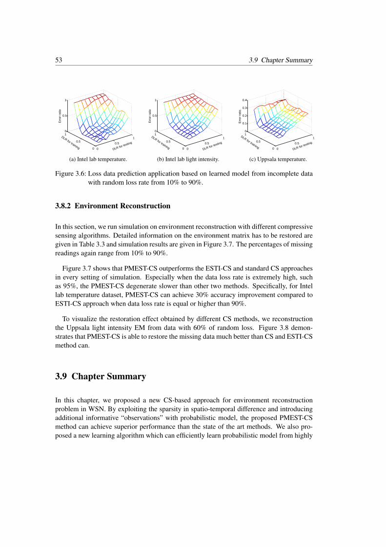
53 3.9 Chapter Summary
0
0.5
1
0
0.5
10
0.5
1
DLR for testing
DLR for training
Err
or r
atio
(a) Intel lab temperature.
0
0.5
1
0
0.5
10
0.5
1
DLR for testing
DLR for trainingE
rror
rat
io
(b) Intel lab light intensity.
0
0.5
1
0
0.5
10
0.1
0.2
0.3
0.4
DLR for testing.
DLR for training.
Err
or r
atio
.
(c) Uppsala temperature.
Figure 3.6: Loss data prediction application based on learned model from incomplete datawith random loss rate from 10% to 90%.
3.8.2 Environment Reconstruction
In this section, we run simulation on environment reconstruction with different compressivesensing algorithms. Detailed information on the environment matrix has to be restored aregiven in Table 3.3 and simulation results are given in Figure 3.7. The percentages of missingreadings again range from 10% to 90%.
Figure 3.7 shows that PMEST-CS outperforms the ESTI-CS and standard CS approachesin every setting of simulation. Especially when the data loss rate is extremely high, suchas 95%, the PMEST-CS degenerate slower than other two methods. Specifically, for Intellab temperature dataset, PMEST-CS can achieve 30% accuracy improvement compared toESTI-CS approach when data loss rate is equal or higher than 90%.
To visualize the restoration effect obtained by different CS methods, we reconstructionthe Uppsala light intensity EM from data with 60% of random loss. Figure 3.8 demon-strates that PMEST-CS is able to restore the missing data much better than CS and ESTI-CSmethod can.
3.9 Chapter Summary
In this chapter, we proposed a new CS-based approach for environment reconstructionproblem in WSN. By exploiting the sparsity in spatio-temporal difference and introducingadditional informative “observations” with probabilistic model, the proposed PMEST-CSmethod can achieve superior performance than the state of the art methods. We also pro-posed a new learning algorithm which can efficiently learn probabilistic model from highly

Chapter 3 Probabilistic Model Enhanced Compressive Sensing for EnvironmentReconstruction in Sensor Networks
54
0 0.2 0.4 0.6 0.8 1
0.1
0.2
0.3
0.4
Data loss probability
Err
or r
atio
CS
ESTI−CS
PMEST−CS
(a) Intel lab temperature.
0 0.2 0.4 0.6 0.8 10.2
0.3
0.4
0.5
0.6
0.7
Data loss probability
Err
or r
atio
CS
ESTI−CS
PMEST−CS
(b) Intel lab light intensity.
0 0.2 0.4 0.6 0.8 10
0.2
0.4
0.6
0.8
1
1.2
Data loss probability
Err
or r
atio
CS
ESTI−CS
PMEST−CS
(c) Uppsala temperature.
0 0.2 0.4 0.6 0.8 10
0.5
1
1.5
Data loss probability
Err
or r
atio
CS
ESTI−CS
PMEST−CS
(d) Uppsala light intensity.
Figure 3.7: Performance of different CS-based algorithms on environment reconstruction.
incomplete data. Experimental results corroborate PMEST-CS method is very efficient andcan achieve significant reconstruction quality gain over the state of the art CS-based meth-ods.

55 3.9 Chapter Summary
Time instance.
Sen
sor
ID.
100 200 300
2
4
6
8
10
12
(a) Original complete data.
Time instance.
Sen
sor
ID.
100 200 300
2
4
6
8
10
12
(b) PMEST-CS restoration.
Time instance.
Sen
sor
ID.
100 200 300
2
4
6
8
10
12
(c) Standard CS restoration.
Time instance.
Sen
sor
ID.
100 200 300
2
4
6
8
10
12
(d) ESTI-CS restoration.
Figure 3.8: Uppsala light intensity data and its restoration with 60% data loss rate by differ-ent CS-based environment reconstruction methods.


Chapter4Rating Network Paths for Locality-AwareOverlay Construction and Routing
This chapter investigates the rating of network paths, i.e. acquiring quantized measures ofpath properties such as round-trip time and available bandwidth. Comparing to fine-grainedmeasurements, coarse-grained ratings are appealing in that they are not only informativebut also cheap to obtain.
Motivated by this insight, we firstly address the scalable acquisition of path ratings bystatistical inference. By observing similarities to recommender systems, we examine theapplicability of solutions to recommender system and show that our inference problem canbe solved by a class of matrix factorization techniques.
Then, we investigate the usability of rating-based network measurement and inference inapplications. A case study is performed on whether locality awareness can be achieved foroverlay networks of Pastry and BitTorrent using inferred ratings. We show that suchcoarse-grained knowledge can improve the performance of peer selection and that finergranularities do not always lead to larger improvements.
Contents4.1 Introduction . . . . . . . . . . . . . . . . . . . . . . . . . . . . . . . 594.2 Related Work . . . . . . . . . . . . . . . . . . . . . . . . . . . . . . . 61
4.2.1 Inference of Network Path Properties . . . . . . . . . . . . . 614.2.2 Locality-Aware Overlay Networks . . . . . . . . . . . . . . . 61
4.3 Properties and Rating of Network Paths . . . . . . . . . . . . . . . . . 624.3.1 Properties of Network Paths . . . . . . . . . . . . . . . . . . 624.3.2 Rating of Network Paths . . . . . . . . . . . . . . . . . . . . 63
4.4 Network Inference of Ratings . . . . . . . . . . . . . . . . . . . . . . 644.4.1 Problem Statement . . . . . . . . . . . . . . . . . . . . . . . 64

Chapter 4 Rating Network Paths for Locality-Aware Overlay Construction and Routing 58
4.4.2 Connections to Recommender Systems . . . . . . . . . . . . 654.4.3 Matrix Factorization . . . . . . . . . . . . . . . . . . . . . . 674.4.4 MF for Network Inference . . . . . . . . . . . . . . . . . . . 704.4.5 Comparison of Different MF Models . . . . . . . . . . . . . . 71
4.5 Case Study: Locality-Aware Overlay Construction and Routing . . . . 764.5.1 Pastry . . . . . . . . . . . . . . . . . . . . . . . . . . . . . . 774.5.2 BitTorrent . . . . . . . . . . . . . . . . . . . . . . . . . . . . 784.5.3 Remarks . . . . . . . . . . . . . . . . . . . . . . . . . . . . . 80
4.6 Chapter Summary . . . . . . . . . . . . . . . . . . . . . . . . . . . . 80

59 4.1 Introduction
4.1 Introduction
Network measurement is a fundamental problem in the heart of the networking research.Over the years, various tools have been developed to acquire path properties such as round-trip time (RTT), available bandwidth (ABW) and packet loss rate, etc [24]. As in mostscientific disciplines, the common sense in the field is that a measurement should be madeas fine-grained and accurate as possible. This is considered necessary to enable quantitativeanalysis of network performance.
However, recent advances in emerging Internet services have created numerous situationswhere coarse-grained measurements can be leveraged and may even be preferred. A typicalexample is Peer-to-Peer (P2P) Overlay Networks [72] where a common design is to useIntelligent Peer Selection to improve traffic locality [41], i.e. encourage more communica-tions between “nearby” nodes, with connections of small RTT or high ABW. The objectiveis thus to find “good-enough” paths for overlay construction and routing, which can be wellserved by using coarse-grained network measurement.
Motivated by this insight, this chapter investigates the rating of network paths, i.e. ac-quiring quantized path properties represented by ordinal numbers of 1,2,3, . . ., with largervalue indicating better performance. Although coarse-grained, ordinal ratings are appealingfor the following reasons:
• Ratings carry sufficient information that already fulfills the requirements of manyapplications.• Ratings are rough measures that are cheaper to obtain than exact property values.• Ratings can be encoded in a few bits, saving storage and transmission costs.
A practical issue of rating-based network measurement is the efficient acquisition on largenetworks. While cheap for a single path, it is still infeasible to rate all paths in a network byactive probing due to the quadratic complexity. The scalability issue has been successfullyaddressed by statistical inference that measures a few paths and predicts the properties ofthe other paths where no direct measurements are made [25–33]. Inspired by these studies,a particular focus of this chapter is network inference of ratings: how ratings of networkpaths can be accurately predicted. An interesting observation is that the inference problemresembles the problem of recommender systems which studies the prediction of preferencesof users to items [40]. If we consider a path property as a “friendship” measure betweenend nodes, then intelligent peer selection can be viewed as a “friend” recommendation task.This seemingly trivial connection has the great benefit to leverage the rapid progresses inmachine learning and investigate the applicability of various solutions to recommender sys-tems for network inference. Our studies show that a class of matrix factorization techniquesare suitable for network inference and achieved good results that are known to be acceptable

Chapter 4 Rating Network Paths for Locality-Aware Overlay Construction and Routing 60
for recommendation tasks.
Another practical issue on rating-based network measurement is the usability in appli-cations. Two questions need to be answered, the first of which is whether the inferenceof ratings is accurate enough to be exploited by applications and the second of which ishow to determine a proper granularity. While a coarser granularity means rougher andthus cheaper measurement, it also means more information losses which may hurt the per-formance of applications. Answers to these questions are critical in the design of systemarchitecture, particularly for P2P applications where the knowledge of locality plays animportant role [35, 41, 42].
Thus, we answer these two questions by investigating quantitatively the impacts of boththe inaccuracy of the inference and the granularity. For the case study, we consider locality-aware overlay construction and routing where locality refers to the proximity between net-work nodes according to some path property such as RTT or ABW. More specifically, weperformed the study on Pastry [42] and BitTorrent [35], which are typical structured and un-structured overlay networks and are known to enjoy the property of locality awareness, andevaluated the performance of overlay construction and routing, with the knowledge of lo-cality obtained via network inference of ratings. Our studies show that while the knowledgeof inferred ratings can improve the performance of peer selection, finer granularities do notalways lead to larger improvements. For example, our simulations on various datasets showthat the performance of peer selection improves very little when the rating level reaches 24.
Thus, this chapter makes the following contributions:
• We investigate the rating-based network measurement that acquires quantized pathproperties represented by ordinal numbers. Such representation not only is informa-tive but also reduces measurement, storage and transmission costs.• We investigate the scalable acquisition of ratings by network inference. We highlight
similarities between network inference and recommender systems and examine theapplicability of solutions from this latter domain to network inference. In particular,we show that our inference problem can be solved by a class of matrix factorizationtechniques.• We perform a case study on locality-aware overlay construction and routing to
demonstrate the usability of rating-based network measurement and inference in P2Papplications.
The rest of the chapter is organized as follows. Section 4.2 introduces related work.Section 4.3 describes the properties and the rating of network paths. Section 4.4 introducesnetwork inference by a class of matrix factorization techniques. Section 4.5 introduces thecase study on locality-aware overlay construction and routing. Section 4.6 gives conclusionsand future work.

61 4.2 Related Work
4.2 Related Work
4.2.1 Inference of Network Path Properties
Network inference has been studied for over a decade, and numerous approaches have beendeveloped. For example, GNP [25] and Vivaldi [26] solved the inference of RTT by Eu-clidean embedding, while tomography-based approaches such as TOM [27], Network Krig-ing [28] and NetQuest [29] used linear algebraic methods and the routing tables to inferadditive properties such as RTT and packet loss rate. Although interesting in different as-pects, these approaches are limited only to certain path properties and/or rely on the routinginformation of the network which is expensive to obtain for applications.
To overcome these constraints, a recent advance was made in [32, 33] that formulatednetwork inference as a matrix completion problem. A class of algorithms called DMFSGDwas proposed and showed improved accuracy and flexibility in dealing with various prop-erties including the non-additive ABW. Matrix completion is suitable for network inferencebecause it exploits the correlations between measurements of different paths [27,28,33,73]and has also been used for other problems such as network traffic estimation [74–76].
All above-mentioned work focused on the prediction of exact measurement values, ex-cept [32] which classified path properties into binary classes of either “good” or “bad”.This chapter goes further and is the first to investigate rating-based network measurementand inference. Ratings are measures in between property values and binary classes: onthe one hand, they are more informative than binary classes; on the other hand, they areadvantageous over property values due to the coarse-grained measurement.
4.2.2 Locality-Aware Overlay Networks
There are two classes of overlay networks: structured and unstructured [72]. The formerplaces content deterministically at specified locations according to the Distributed Hash Ta-ble (DHT) which makes subsequent queries efficient. The latter organizes peers more ran-domly and uses flooding or random walks to query content. Examples of structured systemsare Kademlia [77], Chord [78] and Pastry [42], and those of unstructured are Freenet [79],Gnutella [80] and BitTorrent [35].
For both structured and unstructured overlay networks, a desired property is locality-awareness which makes communications as local as possible. Such a property is importantfor P2P applications because it can reduce cross-domain traffic, avoid congestions and im-prove service performance [41]. It is recognized that locality-awareness can be achieved via

Chapter 4 Rating Network Paths for Locality-Aware Overlay Construction and Routing 62
intelligent peer selection whereby dense connections are enforced between nodes that arewell connected to each other, i.e., short in terms of RTT or wide in terms of ABW. Whilethe effectiveness of intelligent peer selection has been repeatedly justified [41, 81, 82], thischapter is the first to study whether locality-awareness can be achieved, in both structuredand unstructured overlay networks, using rough and inaccurate knowledge of network prox-imity obtained via network inference of ratings.
4.3 Properties and Rating of Network Paths
4.3.1 Properties of Network Paths
While ultimately the performance of a network path should be judged by the quality ofservice (QoS) perceived by end users, it is important to define an objective metric thatis directly measurable without user interventions. Among the commonly-used path prop-erties mentioned earlier, this chapter only discusses round-trip time (RTT) and availablebandwidth (ABW) due to the availability of such data and the relatively rare occurrence ofpackets losses in the Internet [24].
4.3.1.1 Round-Trip Time (RTT)
The RTT is one of the oldest and most commonly-used network measurements due partiallyto its ease of acquisition by using ping with little measurement overhead, i.e., few ICMPecho request and response packets between the sender and the target node. Although theone-way forward and reverse delays are not exactly the same due e.g. to the routing policies,the RTTs between two network nodes can be treated as symmetric.
4.3.1.2 Available Bandwidth (ABW)
The ABW is the remaining capacity of the bottleneck link on a path. Many comparativestudies have shown that tools based on self-induced congestion are generally more accu-rate [24, 83]. The principle states that if the probing rate exceeds the available bandwidthover the path, then the probe packets become queued at some router, resulting in an in-creased transfer time. The ABW can then be estimated as the minimum probing rate thatcreates congestions or queuing delays. To this end, pathload [84] sends trains of UDP pack-ets at a constant rate and adjusts the rate from train to train until congestions are observed

63 4.3 Properties and Rating of Network Paths
at the target node, while pathchirp [85] reduces the probe traffic by varying the probe ratewithin a train exponentially.
Comparing to the RTT, the ABW measurement is much more costly and less accurate.For example, many studies revealed the pitfalls and the uncertainties of the ABW mea-surement [83, 86, 87]. In this chapter, we ignore these measurement issues and investigatehow network inference can be performed1 for ABW using a publicly available dataset [2]in which the measurements were acquired by pathchirp, a fairly accurate and widely-usedtool [83]. In contrast to the RTT, the ABW is asymmetric and its measurement is inferredat the target node.
4.3.2 Rating of Network Paths
Generally, ratings can be acquired by vector quantization that partitions the range of the pathproperty into R bins using R−1 thresholds, denoted by τ = τ1, . . . ,τR−1, and determinesto which bins property values belong. The thresholds can be chosen evenly or unevenlyaccording to the data distribution or the requirements of applications. For example, GoogleTV requires a broadband speed of 2.5Mbps or more for streaming movies and 10Mbps forHigh Definition contents [88]. Accordingly, τ = 2.5Mbps,10Mbps can be defined forABW to separate paths of rating 1, 2 and 3.
Rating by quantization is directly applicable to RTTs whose measurements are cheap. Forthe ABW, it is preferable to directly obtain the rating measures without the explicit acquisi-tion of the values in order to reduce measurement overhead. In general, as data acquisitionundergoes the accuracy-versus-cost dilemma, stating that accuracy always comes at a cost,coarse-grained measurements are always cheaper to obtain than fine-grained ones. The ad-vantage of the low measurement cost holds particularly for ABW whose measurement iscostly.
Note that when R = 2, rating degenerates to binary classification of network paths whichwas studied in [32]. When R is very large, rating approaches the measurement of propertyvalues, which was studied in [33]. Thus, R results from a trade-off between the granularityand the measurement costs. A larger R means finer granularity but at the cost of moremeasurement overheads, and vice versa. Nevertheless, we will fix R = 5 in Section 4.4where we examine the applicability of solutions to recommender systems. Such a choice isnatural because it corresponds to the commonly-used 5-star rating system which categorizesperformance into 5 discrete levels of “very poor”, “poor”, “ordinary”, “good” and “verygood” quality . We will study the impact of different choices of R in Section 4.5.
1Strictly speaking, we do not infer the property of a path. Instead, we infer the property value that should havebeen obtained by some measurement tool.

Chapter 4 Rating Network Paths for Locality-Aware Overlay Construction and Routing 64
11
2
2
3
3
4
4
5
5
6
6
7
7
8
8
3
1 2
45
6 7
83
1 2
6
8
(a) Node 3 probes node 1, 2, 6 and 8.
11
2
2
3
3
4
4
5
5
6
6
7
7
8
8
3
1 2
45
6 7
83
1 2
6
83
5
2
8
4
7
5
(b) A matrix with some missing entries is formed.
Figure 4.1: A matrix completion view of network inference. In (b), the blue entries aremeasured path properties and the green ones are missing. Note that the diagonalentries are empty as they represent the performance of the path from each nodeto itself which carries no information.
4.4 Network Inference of Ratings
This section describes the scalable acquisition of ratings on large networks by statisticalinference.
4.4.1 Problem Statement
Formally, the inference problem is stated as follows. Consider a network of n end nodes, anddefine a path to be a routing path between a pair of end nodes. There are O(n2) paths in thenetwork, and we wish to monitor a small subset of paths so that the performance of all other

65 4.4 Network Inference of Ratings
paths can be estimated. Note that here we seek to infer ratings, instead of values, of pathproperties. Besides reducing the measurement overheads, another motivation of networkinference is that we can estimate the properties of those paths which are not measurable duee.g. to the lack of experimental controls.
This inference problem has a matrix completion form where a partially observed matrixis to be completed [89]. In this context, a matrix, denoted by X , is constructed, with itsentry xi j being the rating of the path from node i to node j. Each node randomly probes afew other nodes and measures the ratings of the paths to them. The measurements are put inthe corresponding entries of X , and the missing entries are the ratings of those unmeasuredpaths and need to be estimated, illustrated in Figure 4.1. Note that X is a square matrixwhen it contains the performance of all pairwise paths in a network. However, for situationswhere one set of nodes in a network probe another set of nodes in the same or a differentnetwork, X becomes non-square. Such situations arise in content distribution networks(CDNs) where a set of users probe a set of servers [90].
In order for network inference to be feasible, network measurements on different pathshave to be correlated with or dependent on each other. Otherwise, the inference would beimpossible or suffer from large errors, regardless the inference schemes used. The correla-tions between network measurements exist, because Internet paths with nearby end nodesoften overlap or share bottleneck links due to the simple topology of the Internet core. Theredundancy of link usage across paths causes the performance of many paths to be corre-lated [27–29]. For example, the congestion at a certain link causes the delays of all pathsthat traverse this link to increase jointly. A direct consequence of such correlations is thatthe related performance matrix occurs to have a low-rank characteristic [33, 73] which fur-ther enables the inference problem to be solved by matrix factorization techniques, shownin the following sections. The low-rank characteristic of performance matrices of RTT andABW is illustrated by the spectral plots in Figure 4.2. It can be seen that the singularvalues of these matrices decrease fast, which is an empirical justification of the low-rankphenomenon.
4.4.2 Connections to Recommender Systems
The problem of network inference bears strong similarities to the problem of recommendersystems which predicts the preference of users to items such as music, books, or movies [40,91]. Table 4.1 shows an example of a recommender system. Consider that network nodesare users and that each node treats other nodes as items or “friends”. The performance ofa network path is then actually a “friendship” measure of how one end node would like tocontact the other end node of the path. In particular, the task of intelligent peer selection canbe viewed as a “friend” recommendation task. Guided by this insight the rapid advances

Chapter 4 Rating Network Paths for Locality-Aware Overlay Construction and Routing 66
1 5 10 15 200
0.2
0.4
0.6
0.8
1
# singular value
sin
gu
lar
va
lue
s
RTT
RTT ratings
ABW
ABW ratings
Figure 4.2: The singular values of a 2255×2255 RTT matrix, extracted from the Meridiandataset [1], and a 201×201 ABW matrix, extracted from the HP-S3 dataset [2],and of their corresponding rating matrices. The rating matrices are obtained bythresholding the measurement matrices with τ = 20%,40%,60%,80% per-centiles of each dataset. The singular values are normalized so that the largestones equal 1.
made for recommender systems can be applied to our inference problem.
Table 4.1: An example of a recommender system.item1 item2 item3 item4 item5 item6
user1 5 3 4 1 ? ?user2 5 3 4 1 5 2user3 5 ? 4 1 5 3user4 1 3 2 5 1 4user5 4 ? 4 4 4 ?
In particular, research on recommender systems was largely motivated by the Netflix prizewhich was an open competition initiated in 2006 for algorithms that predict the preference,quantized by the 5-star rating system, of users to movies [92]. A grand prize of one milliondollar was to be given to the first algorithm that improves the accuracy of Netflix’s ownalgorithm cinematch by 10%. The prize had attracted a lot of efforts and attempts before itwas given to the BellKor’s Pragmatic Chaos team in 2009 which achieved an improvementof 10.21%. In what follows, the prize-winning solution is called BPC. Specifically, BPCintegrated two classes of techniques based on neighborhood models and on matrix factor-

67 4.4 Network Inference of Ratings
ization. Neighborhood models exploit the similarities between users and between items.For example, two users are considered similar if they rate a set of items similarly. Mean-while, two items are considered similar if they are given similar ratings by a set of users.Although interesting, neighborhood models are infeasible for network inference, because,to compute the similarities between network nodes, they must probe a number of commonnodes, which is impossible when the nodes being probed are randomly selected2. Thus, wefocus below on the matrix factorization models in BPC.
4.4.3 Matrix Factorization
Matrix factorization (MF) exploits the low-rank nature of matrices of real-world data. Math-ematically, a n by n matrix of rank r, where r n, has only r non-zero singular values andit can be factorized as
X =UV T , (4.4.1)
where U and V are matrices of size n× r. In practice, due to data noise, X is often full-rankbut with a rank r dominant component. That is, X has only r significant singular values andthe other ones are negligible. In this case, a rank-r matrix X can be found that approximatesX with high accuracy, i.e.,
X ≈ X =UV T . (4.4.2)
MF can be used for solving the problem of matrix completion, which generally minimizesan objective function of the following form:
min ∑i j∈Ω
l(xi j,uivTj ), (4.4.3)
where Ω is the set of observed entries, xi j is the i jth entry of X , and ui and v j are the ith andjth row of U and of V respectively. l is a loss function that penalizes the difference betweenthe two inputs. In words, we search for (U,V ) so that X =UV T best approximates X at theobserved entries in Ω . The unknown entries in X are predicted by
xi j = uivTj , for i j /∈Ω . (4.4.4)
Note that xi j is real-valued and has to be rounded to the closest integer in the range of 1,Rfor ordinal rating. Figure 4.3 illustrates MF for matrix completion.
Below, we introduce various MF models that were integrated in BPC including RMF,MMMF and NMF.
2However, if we accept to depart from a fully distributed solution to the problem, it is possible to deploy somelandmark nodes in the network for other nodes to probe. Thus, each node knows its performance informationto/from the common landmarks. In such situations, the neighborhood models become applicable and areinteresting to study, which is left as future work.

Chapter 4 Rating Network Paths for Locality-Aware Overlay Construction and Routing 68
X
uivTj = xij ≈ xij
X≈xij xij
Uui
V T
vTj
Figure 4.3: Matrix factorization.
4.4.3.1 RMF
Regularized matrix factorization (RMF) [40] adopts the widely-used square loss functionand solves
min ∑i j∈Ω
(xi j−uivTj )
2 +λ
n
∑i=1
(uiuTi + vivT
i ). (4.4.5)
The second term is the regularization which restricts the norm of U and V so as to preventoverfitting, and λ is the regularization coefficient.
4.4.3.2 MMMF
Max-margin matrix factorization (MMMF) solves the inference problem by ordinal regres-sion [93] which relates the real-valued estimate xi j to the ordinal rating xi j by using R− 1thresholds θ1, . . . ,θR−1. More specifically, MMMF requires the following constraint tobe satisfied for each xi j, i j ∈Ω ,
θc−1 < xi j = uivTj 6 θc, for xi j = c, 1 6 c 6 R. (4.4.6)
For simplicity of notation θ0 =−∞ and θR =+∞. In words, the value of xi j does not matter,as long as it falls in the range of θc−1,θc for xi j = c, 1 6 c 6 R. Here we set the thresholdsas 1.5,2.5,3.5,4.5 for R = 5. Thus, the constraint in eq. 4.4.6 means that, for example, ifxi j = 2, then it is required that 1.5 < xi j < 2.5 so that xi j will be rounded to 2. Whether xi j
is 2, 2.2 or 1.6 makes no difference.

69 4.4 Network Inference of Ratings
Thus, we penalize the violation of the constraint in eq. 4.4.6 for each xi j and minimizethe following objective function
min ∑i j∈Ω
R−1
∑c=1
l(T ci j,θc−uivT
j )+λ
n
∑i=1
(uiuTi + vivT
i ), (4.4.7)
where T ci j = 1 if xi j > c and −1 otherwise. Essentially, the objective function in eq. 4.4.7
consists of R− 1 binary classification losses, each of which compares an estimate xi j witha threshold θc in θ1, . . . ,θR−1. For example, for xi j = 2, it is required that xi j > 1.5and xi j < 2.5, xi j < 3.5, xi j < 4.5. Each violation of these four constraints is penalized byl(T c
i j,θc−uivTj ), with
T ci j =
−1 for c = 11 for 2 6 c 6 4
(4.4.8)
indicating the correct sign of (θc−uivTj ).
Note that l in eq. 4.4.7 can be any classification loss function, among which the smoothhinge loss function is used [93], defined as
l(x, x) =
0 if xx > 1
12(1− xx)2 if 0 < xx < 1
12 − xx if xx 6 0
(4.4.9)
4.4.3.3 NMF
Non-negative matrix factorization (NMF) [94] incorporates an additional constraint that allentries in U and V have to be non-negative so as to ensure the non-negativity of X . Besides,NMF uses the divergence as the loss function, defined as
D(X ||X) = ∑i j∈Ω
(xi jlogxi j
xi j− xi j + xi j). (4.4.10)
Thus, NMF solves
minD(X ||UV T )+λ
n
∑i=1
(uiuTi + vivT
i ), s.t. (U,V )> 0. (4.4.11)
4.4.3.4 MF Ensembles
Instead of using one of these MF models, BPC integrated all of them in an ensemble frame-work, which is the root of its success. The idea is to learn multiple predictors simulta-neously, by using different MF models (RMF, MMMF and NMF) and by setting different

Chapter 4 Rating Network Paths for Locality-Aware Overlay Construction and Routing 70
parameters for each MF model, and combines their outputs, by voting or averaging, forprediction [95, 96]. Intuitively, the power of ensemble methods comes from the “wisdomof the crowd”, which says that a large group’s aggregated answer to a question is generallyfound to be as good as, and often better than, the answer given by any of the individualswithin the group [97].
Besides improving accuracy, ensemble models allow to compute the variance of eachprediction, by computing the variance of the predictions by different predictors. Varianceindicates the uncertainty of the prediction: large variance means that different predictorsdisagree with each other and we are thus less certain about the combined prediction3. Suchinformation can be exploited in e.g. intelligent peer selection so that we can choose, amongnodes with high ratings, those with small variance as they are more certain.
4.4.4 MF for Network Inference
4.4.4.1 Inference By Stochastic Gradient Descent
We adopted Stochastic Gradient Descent (SGD) for solving all MF models. In short, wepick xi j in Ω randomly and update ui and v j by gradient descent to reduce the differencebetween xi j and uivT
j . SGD is particularly suitable for network inference, because mea-surements can be acquired on demand and processed locally at each node. We refer theinterested readers to [32, 33] for the details of the inference by SGD.
4.4.4.2 Neighbor Selection
We also adopted the common architecture that each node randomly selects k nodes to probe,called neighbors in the sequel. That is, each node measures the properties of the paths fromitself to the k neighbors and predicts the other paths by using MF-based inference schemes.
The choice of k is the result of a trade-off between accuracy and measurement overhead.On one hand, increasing k always improves accuracy as we measure more and infer less.On the other hand, the more we measure, the higher the overhead is. Thus, we vary k fornetworks of different sizes so as to control the number of paths being monitored to be acertain percentage of the total number of paths in a network. In particular, we require kto be no smaller than 10 so that a certain amount of information about the performance
3While we build our confidence on the variance of a prediction, it does not mean that smaller variance leadsto better accuracy. Instead, it means that the combined prediction makes more sense if the variance is small,i.e. if different predictors agree with each other.

71 4.4 Network Inference of Ratings
at each node is guaranteed. This leads to less than 5% of available measurements for anetwork of about two hundred nodes, which is the smallest dataset we used in the chapter.For large networks of a few thousand nodes, we increase k so that about 1% of the paths aremonitored. As the largest dataset we used in this chapter has less than 5000 nodes, k is nolarger than 50. We consider that such setting of k leads to sparse available measurementsthat is affordable for large networks.
4.4.4.3 Rank r
The rank r is an important parameter and can only be determined empirically. On the onehand, r has to be large enough so that the dominant components in X are kept. On theother hand, a higher-rank matrix has less redundancies and requires more data to recover,increasing measurement overheads. Our experiments show that empirically, r = 10 is agood choice, given the sparse available measurements.
4.4.5 Comparison of Different MF Models
This section compares different MF models on our network inference problem. In the eval-uations, we set R = 5, which was also used in the Netflix prize.
The comparison was then performed on the following publicly available datasets:
• Harvard contains dynamic RTT measurements, with timestamps, between 226Azureus clients deployed on PlanetLab [98];• Meridian contains static RTT measurements between 2500 network nodes obtained
from the Meridian project [1];• HP-S3 contains static ABW measurements between 231 PlanetLab nodes [2].• YouTube contains static RTT measurements from 441 PlanetLab nodes to 4816
YouTube servers [90].
In the simulations, the static measurements in Meridian, HP-S3 and YouTube are used inrandom order, whereas the dynamic measurements in Harvard are used in time order ac-cording to the timestamp of each measurement.
We adopted the evaluation criterion, Root Mean Square Error (RMSE), given by
RMSE =
√∑
ni=1(xi− xi)2
n. (4.4.12)

Chapter 4 Rating Network Paths for Locality-Aware Overlay Construction and Routing 72
which was used in the Netflix prize. As RMSE is the average estimation error, the smallerit is, the better.
4.4.5.1 Obtaining Ratings
The first step is to obtain ratings on a scale of 1,5 from the raw measurements. To thisend, the range of a path property is partitioned by the rating threshold τ = τ1, . . . ,τ4. τ isset by two strategies:
• Strategy 1: set τ by the 20%,40%,60%,80% percentiles of each dataset.
– Harvard: τ = 48.8,92.2,177.2,280.3ms– Meridian: τ = 31.6,47.3,68.6,97.9ms– HP-S3: τ = 12.7,34.5,48.8,77.9Mbps– YouTube: τ = 38.1,91.1,131.3,192.4ms
• Strategy 2: partition evenly the range between 0 and a large value manually selectedfor each dataset.
– Harvard: τ = 75,150,225,300ms– Meridian: τ = 25,50,75,100ms– HP-S3: τ = 20,40,60,80Mbps– YouTube: τ = 50,100,150,200ms
4.4.5.2 Results
Throughout the chapter, the MF parameters are set as follows: for RMF, MMMF and NMF,the regularization coefficient λ = 0.1 and the rank r = 10. For MF ensembles, we generatedfor each MF model (RMF, MMMF and NMF) 6 predictors using different parameters, i.e.r ranges from 10 to 100 and λ ranges from 0.01 to 1, as described in [96]. For the neighbornumber, k = 10 for Harvard of 226 nodes, leading to about 4.42% available measurements;k = 32 for Meridian of 2500 nodes, leading to about 1.28% available measurements; k =10 for HP-S3 of 231 nodes, leading to about 4.33% available measurements; k = 50 forYouTube of 4816 servers, leading to about 1.04% available measurements. Thus, we collectk measurements at each node and perform the inference using different MF models. Theevaluation was done by comparing the inferred ratings of those unmeasured paths with theirtrue ratings, calculated by RMSE defined above.
Table 4.2 shows the RMSEs achieved by different MF models and on different datasets.We can see that while RMF generally outperforms MMMF and NMF, MF ensembles per-

73 4.4 Network Inference of Ratings
form the best at the cost of more computational overheads due to the maintenance of multi-ple MF predictors. Note that all MF models achieved fairly accurate results with the RMSEless than 1. In comparison, for the dataset in the Netflix prize, the RMSE achieved by theNetflix’s cinematch algorithm is 0.9525 and that by BPC is 0.8567 [92]. While the RMSEson different datasets are not comparable, it shows that in practice, the prediction with anaccuracy of the RMSE less than 1 for ratings on a scale of 1,5 is already accurate enoughto be used for recommendation tasks. Note that from Table 4.2, it appears that Strategy 2which partitions the range of the property evenly produced smaller RMSEs than Strategy 1which set τ by certain percentiles of the data. However, the RMSEs by different strategiesare not comparable, because the evaluations were performed on different rating data gen-erated by different strategies. Nevertheless, Strategy 2 may create unbalanced portions ofratings. For example, we may have no path of rating 1 but a lot of paths of rating 2, whichwill never occur for Strategy 1. For this reason, Strategy 1 is used by default in the rest ofthe chapter.
Table 4.2: RMSE on different datasets.τ: Strategy 1 Harvard Meridian HP-S3 YouTube
RMF 0.934 0.831 0.675 0.923MMMF 0.969 0.863 0.686 0.957
NMF 0.977 0.904 0.682 0.969MF Ensembles 0.920 0.821 0.661 0.901τ: Strategy 2 Harvard Meridian HP-S3 YouTube
RMF 0.920 0.776 0.669 0.910MMMF 0.919 0.810 0.670 0.944
NMF 0.932 0.829 0.674 0.961MF Ensembles 0.904 0.766 0.653 0.873
Overall, RMF is lightweight and suits well for online deployment in P2P applications, andis thus used in Section 4.5 for the case study on overlay construction and routing. Table 4.3shows the confusion matrices achieved by RMF on the four datasets. In these matrices, eachcolumn represents the predicted ratings, while each row represents the actual ratings. Thus,the diagonal entries represent the percentage of the correct prediction, and the off-diagonalentries represent the percentage of “confusions” or mis-ratings. For example, the entry at(2,2) represents the percentage of the rating-2 paths which are correctly predicted as rating-2, and the entry at (2,3) represents the percentage of the rating-2 paths which are wronglypredicted as rating-3, i.e. the confusions from rating-2 to rating-3. It can be seen that whilethere are mis-ratings, most of them have a small error of |xi j− xi j| = 1, marked as shadedentries in the confusion matrices in Table 4.3. This means that the mis-ratings are undercontrol. For example, a rating-5 path may be wrongly predicted as 4, but seldom as 3, 2 or

Chapter 4 Rating Network Paths for Locality-Aware Overlay Construction and Routing 74
1, since the entries at (5,3), (5,2) and (5,1) in all confusion matrices are small.
Table 4.3: Confusion matrices.
HarvardPredicted
1 2 3 4 5
Actual
1 68% 28% 2% 1% 1%2 18% 60% 20% 1% 1%3 3% 13% 66% 17% 1%4 3% 4% 16% 67% 10%5 3% 3% 5% 43% 46%
MeridianPredicted
1 2 3 4 5
Actual
1 78% 18% 3% 1% 0%2 8% 59% 30% 3% 0%3 1% 18% 60% 20% 1%4 1% 3% 33% 59% 4%5 1% 1% 12% 59% 27%
HP-S3Predicted
1 2 3 4 5
Actual
1 92% 6% 1% 1% 0%2 11% 65% 22% 2% 0%3 1% 20% 68% 11% 0%4 0% 3% 33% 58% 6%5 0% 1% 10% 55% 34%
YouTubePredicted
1 2 3 4 5
Actual
1 80% 17% 1% 1% 1%2 13% 66% 20% 1% 0%3 2% 13% 69% 15% 0%4 3% 8% 33% 52% 4%5 2% 7% 12% 46% 32%
Note that we also evaluated another matrix completion method, namely LMaFit4, whichwas used in [74] for traffic matrix completion and found that it performed much worse thanthe MFs used in this chapter. For example, the RMSE by LMaFit on Meridian, HP-S3and YouTube are 1.357, 1.139 and 1.422 respectively. Note also that many general matrixcompletion methods including LMaFit take as input an incomplete matrix and make updates
4The source code is downloaded from http://lmafit.blogs.rice.edu/.

75 4.4 Network Inference of Ratings
on the entire matrix. This means that they can not process the dynamic measurements in theHarvard dataset, nor can they be decentralized. It is however worth mentioning that LMaFitruns much faster than the MFs based on SGD.
4.4.5.3 Observations
Our experiments reveal a useful effect of ordinal rating. In practice, MF is known to besensitive to outliers such as those unusually large and small values in the datasets. However,as ratings are quantized measures, measurement outliers are naturally handled by truncatingthe large and small property values to 1 and R. A direct consequence is that MF becomesinsensitive to parameter settings, as the inputs are always in a relatively small and fixedrange.
In the experiments, we observed that there exist nodes which have a poor rating with alltheir k neighbors. The likely reason is that those nodes have a poor access link, i.e. thelink by which a node is connected to the Internet core is the bottleneck, which causes allconnected paths to perform poorly. Thus, we calculate the mean rating and the standarddeviation of the measured paths associated with each node, denoted by µi and σi. If σi issmall, we do not consider that node i provides useful information about the performanceof the network, and will simply predict the ratings of all paths of node i as µi. In ourdatasets, the non-informative nodes are rare (i.e. no more than 10 in each dataset), and thusthe “mean rating” trick improved the accuracy only slightly. However, we incorporate it todetect non-informative nodes so that they won’t pose a problem in any case.
4.4.5.4 Discussions on Scalability
The MF models have proved to work well for recommender systems on extremely largematrices such as the one in the Netflix prize. Thus, there is no scalability issue when run-ning MFs on performance matrices constructed on networks even with millions of nodes.However, two practical questions need to be answered when deploying MFs on real, largenetworks:
• How many measurements are required to make predictions with a decent accuracy,i.e., an RMSE at least smaller than 1?• How fast do MFs run on such a large matrix?
Regarding the first question, a theory in matrix completion states that a n×n matrix of rankr can be exactly or accurately recovered, with high probability, from as few as O(nrlog(n))randomly sampled entries [89]. This means that each node would have to probe O(rlog(n))

Chapter 4 Rating Network Paths for Locality-Aware Overlay Construction and Routing 76
neighbors, which scales fairly well in theory. Nevertheless, we are interested in evalu-ating whether such a bound holds or is required for MF-based network inference on largenetworks. Regarding the second question, it is known that MFs based on SGD are computa-tionally efficient, as SGD involves only vector operations [32,33], and empirically convergefast for large matrices, as demonstrated in BPC. We leave the study of these issues as futurework, because it would require really large-scale network measurement data.
4.5 Case Study: Locality-Aware Overlay Construction andRouting
With the techniques of rating-based network measurement and inference presented above,the remaining issue is the usability in Internet applications. There are two questions to beanswered:
• While Section 4.4.5 shows that the inference by various MF models can achieve atleast an accuracy of RMSE less than 1, it is natural to ask whether such an accuracyis acceptable for applications.• It is critical to choose a proper granularity for rating network paths, because although
a finer granularity leads to more informative measurement, it also means more mea-surement overheads which may overweigh the benefit of exploiting the knowledge ofnetwork proximity. Thus, it is also natural to ask whether more fine-grained ratingsalways improve the performance of applications.
To answer these questions, we perform a case study on locality-aware overlay construc-tion and routing and investigate whether locality-awareness can be achieved by using in-ferred ratings of path properties such as RTT and ABW. More specifically, we consider Pas-try [42] and BitTorrent [35] which are typical structured and unstructured overlay networksand are known to enjoy the property of locality-awareness. Both Pastry and BitTorrent relyon an outside program that acquires network path properties. For example, Pastry uses mea-surement tools such as traceroute for hop count or ping for RTT [42], and BitTorrent usesVivaldi to infer RTTs [98]. Here, we are interested in knowing whether our MF-based in-ference schemes can serve as the outside program in Pastry and BitTorrent5 and the impactof the rating granularity on their performance. To simplify the evaluation, we only employ
5Note that investigating how MF-based inference can actually be incorporated in the Pastry and BitTorrentprotocols is beyond the scope of this chapter. However, [32, 33] showed that MF can be implemented ina fully decentralized manner, with the same architecture as Vivaldi [26] which has been incorporated inBitTorrent [98]. This indicates that our MF-based inference schemes can be seamlessly used in BitTorrent,with no extra overhead required. We refer the interested readers to [32,33] for the details of the decentralizedarchitecture and implementations of our MF-based inference schemes.

77 4.5 Case Study: Locality-Aware Overlay Construction and Routing
RMF in this section due to its accuracy and simplicity which facilitates its deployment inP2P applications.
4.5.1 Pastry
Pastry is a classic structured overlay network for the implementation of a DHT where thekey-value pairs are stored in a P2P network in an organized manner so that queries can beachieved within O(logn) hops of routing, where n is the number of nodes. Here, we dropthe description but refer the interested readers to [42] for the construction and routing algo-rithms of Pastry. We mention that Pastry determines the best routes by using the proximityknowledge.
In the simulations, we predicted ratings using RMF on the same datasets and with thesame configuration as described in Section 4.4.5, except that we varied the rating levelsfrom R = 2, R = 22,..., to R = 28, instead of R = 5 in the previous sections. For comparison,we also ran RMF to predict values of path properties, which is the most fine-grained mea-sure. We then built the routing tables in Pastry using respectively no proximity knowledge,inferred ratings, inferred values, as well as the true measurements in the original datasets.We refer to Pastry using no proximity knowledge as R = 0 and using inferred values asR = ∞. Pastry using true measurements is the ideal case where the best routes can be foundat the cost of O(n2) active measurements. In the implementation of Pastry, considering thatthere are at most 2500 nodes in our datasets, the node Id space is N = 214. Other parametersare: the base is B = 2, the leaf set size is L = 2B, the neighbor set size is M = 2B+1, and therouting table size is T = (logL N,L−1) = (7,3).
After construction, we simulated 100,000 lookup messages, i.e. queries, which wererouted from randomly chosen nodes with randomly chosen keys. Then, we compared therouting performance of Pastry under R = 0,21, . . . ,28,∞ respectively with that of usingtrue measurements. We measured the routing performance as the average of a routing met-ric, RTT for Harvard and Meridian and ABW for HP-S3, of each query and calculated theratio between the different cases of R and the ideal case of using true measurements, calledstretch. As Pastry can find the best routes when using true measurements, stretch for therouting performance is greater than 1 for RTT and smaller than 1 for ABW. The closer it isto 1, the better.
Figure 4.4 shows the stretches of both the routing performance and the hop count. Wemake the following observations. First, the stretch of the hop count is very close to 1,which is expected because Pastry always produces routes of O(logn) hops, with or withoutusing the proximity knowledge. Second, also as expected, the routing performance of usinginferred knowledge is worse than that of using true measurements, but is better than using

Chapter 4 Rating Network Paths for Locality-Aware Overlay Construction and Routing 78
no knowledge at all (R = 0), even for the case of R = 2 which leads to the most coarse-grained ratings. This shows that network inference of ratings is accurate enough to beused in Pastry. Third, increasing R after R reaches 23 or 24 cannot further improve therouting performance of Pastry. This shows that rating with finer granularities is not alwaysbeneficial for applications, let alone the extra costs due to more fine-grained measurements.Last, the routing performance of using inferred values (R = ∞) is a little worse than thatof using inferred ratings with R = 24. This seems to suggest that the inference of propertyvalues was affected by measurement outliers, which further degraded the performance ofPastry. In contrast, outliers were naturally filtered out by rating-based measurements.
Harvard Meridian HP-S3
1
1.2
1.4
1.6
1.8
0 21 22 23 24 25 26 27 28 ∞ R
Str
etch
RTTHop Counts
1
1.5
2
2.5
3
0 21
22
23
24
25
26
27
28 ∞
R
Str
etch
RTTHop Counts
0.6
0.7
0.8
0.9
1
1.1
0 21
22
23
24
25
26
27
28 ∞
R
Str
etch
ABWHop Counts
Figure 4.4: Stretch of the routing performance of Pastry, defined as the ratio between therouting metric of Pastry using inferred ratings and of Pastry using true measure-ments. Note that R = 0 means that no proximity knowledge is used, and R = ∞
means that inferred values are used.
4.5.2 BitTorrent
BitTorrent is perhaps the most popular unstructured overlay network and is widely usedfor file sharing [35]. The protocol adopts a random peer selection procedure which causeslarge inter-domain traffic and degrades application performance. It is well known that theseissues can be overcome by intelligent peer selection with the use of the proximity knowledge[41, 81, 82].
In the simulations, we inferred ratings and values of path properties using RMF as de-scribed in the above section. Then, we constructed overlay networks in BitTorrent with astandard scheme whereby a tracker node randomly proposes to each peer 50 peers in thenetwork, among which 32 are selected. Ideally, we would like to connect each peer withthose best performing peers, i.e. shortest for RTT and widest for ABW. However, such bestpeer selection strategy leads to the problem of reachability that some nodes are not reach-

79 4.5 Case Study: Locality-Aware Overlay Construction and Routing
Harvard Meridian HP-S3
100
120
140
160
180
200
220
21 22 23 24 25 26 27 28 ∞ true R
RT
T(m
s)
best100%best90%best50%best0%
60
70
80
90
21 22 23 24 25 26 27 28 ∞ true R
RT
T(m
s)
best100%best90%best50%best0%
50
55
60
65
21 22 23 24 25 26 27 28 ∞ true R
AB
W(M
bps)
best100%best90%best50%best0%
Figure 4.5: Performance of peer selection for BitTorrent, calculated as the average link per-formance between each pair of selected peers. Note that “true” means that truemeasurements are used.
able by some other nodes6. Our simulations showed that there could be 10%∼ 15% of theend-to-end obstructed paths. To overcome this problem, we came up with a mixed strategywhereby p% of the peers execute best peer selection and the other ones execute randompeer selection, referred to as best p% peer selection7. We tested p = 100,90,50,0, withp = 100 being essentially the strategy of best peer selection and p = 0 being random peerselection. Note that the reachability problem is already avoided when p = 90.
We measured the performance of peer selection by the average performance of the linksbetween each pair of peers selected by the peer selection procedure, shown in Figure 4.5.It can be seen that the performance of peer selection improves as more nodes execute thestrategy of best peer selection. This shows that we can reduce download time or avoidcongestions in BitTorrent by exploiting inferred ratings of RTT or ABW. It can also be seenthat, while R = 24 or 25 appear to be optimal, which is similar to Pastry, the granularityseems to have less impact on BitTorrent. This is probably due to the protocol that requireseach peer to select 32 peers out of 50 candidates, thus leaving us with limited choices forpeer selection. Note that BitTorrent is particularly concerned with the performance of peerselection, because chunks of files are frequently exchanged between direct neighbors.
6In an overlay network, the links between nodes are directed. For example, there may be a link from A toB, because A chooses B as its neighbor. However, there may not be a link from B to A, because B maynot choose A as its neighbor. Thus, the problem of reachability doesn’t mean that the overlay network isdisconnected. Instead, it means that some end-to-end paths are obstructed and that packets can only berouted in one direction between some end nodes.
7An alternative strategy for best p% peer selection is to let each node select p% best peers and (100− p)%random peers. We tested both strategies and found that they achieved statistically similar results.

Chapter 4 Rating Network Paths for Locality-Aware Overlay Construction and Routing 80
4.5.3 Remarks
Our case study is encouraging, showing that inferred ratings are accurate enough to be ben-eficial to applications such as Pastry and BitTorrent. Empirically, a coarse granularity ofR = 24 appears to be satisfactory for our datasets, which is acceptable for RTT whose mea-surement is cheap. However, for ABW, the improvement by increasing R from 23 to 24
comes at the cost of more probe flows and thus more overheads, which may not be consid-ered worthy. In practice, the choice of R has to take into account not only the performanceof applications but also the measurement budget.
We measured the inference accuracy by RMSE which reflects the overall accuracy of theprediction for each path. Such metric is more meaningful for applications where the infer-ence accuracy of every path is equally important. For the task of intelligent peer selectionwhere it is only important to ensure that the selected paths have a high rating, it may not beworth pushing the metric of RMSE to the limit. This insight shows that a prediction systemshould be evaluated from the applications’ point of view, which highlights the importanceof carrying out case studies on real applications.
Note that the case study focused on the impact of the accuracy of rating inference andthe impact of the granularity in rating-based network measurement. Thus, we performedno comparison with other inference approaches, as none can deal with ratings of differentpath properties. For example, Vivaldi [26] infers RTT values by Euclidean embedding andwas already shown to be less accurate than our MF-based approach when using the sameamount of RTT measurements [33]. Tomography-based approaches [27–29] do not workon non-additive properties such as ABW and require the routing information of the networkwhich is not available in our scenarios. In contrast, our MF-based approach is flexible indealing with both additive and non-additive properties and in dealing with both propertyvalues and ratings of different levels, which is a unique feature that distinguishes it from allprevious approaches.
4.6 Chapter Summary
This chapter presents a novel concept of rating network paths, instead of measuring valuesof path properties, and investigates the inference of ratings by solutions designed for rec-ommender systems, particularly by a class of matrix factorization techniques, which werefound to work well. The case study on locality-aware overlay construction and routinghighlights the usability of rating-based network measurement and inference by Internet ap-plications. These studies reveal the advantages of ratings: they are informative, have lowmeasurement cost and are easy to process in applications.

Chapter5Conclusion
This thesis demonstrate that novel data interpolation methods can make original expensiveand, even, unobtainable data collection tasks become affordable and feasible. Three specificproblems are considered.
We revisit the AS path inference problem from the complex network perspective. Abrand new constraint is proposed based on the fact the AS paths respect the underlyinggeometric structure of the Internet. Resulting two new AS path inference algorithms, Hy-perPath and Valley-free HyperPath, have O(K) complexity to infer certain end-to-end ASpath and can run locally. Intensive evaluation on the ground truth AS paths shows thatHyperPath method can not only outperform no policy method, it can be superior to ASrelationships based method by being blind to the AS relationships information. The Valley-free HyperPath method outperforms both AS relationships based method and KnownPathmethod. Moreover, two new algorithms are immune to the fail-to-detect problem, by whichthe benchmark methods are always haunted. We also simulate BitTorrent P2P applicationsto show the potential of our methods on inter-domain Internet traffic reduction.
We proposed a new CS-based approach for environment reconstruction problem inWSN. By exploiting the sparsity in spatio-temporal difference and introducing additionalinformative “observations” with probabilistic model, the proposed PMEST-CS method canachieve superior performance than the state of the art methods. We also proposed a newlearning algorithm which can efficiently learn probabilistic model from highly incompletedata. Experimental results corroborate PMEST-CS method is very efficient and can achievesignificant reconstruction quality gain over the state of the art CS-based methods.
We presents a novel concept of rating network paths, instead of measuring values of pathproperties, and investigates the inference of ratings by solutions designed for recommendersystems, particularly by a class of matrix factorization techniques, which were found towork well. The case study on locality-aware overlay construction and routing highlights

Chapter 5 Conclusion 82
the usability of rating-based network measurement and inference by Internet applications.These studies reveal the advantages of ratings: they are informative, have low measurementcost and are easy to process in applications.

Bibliography
[1] Bernard Wong, Aleksandrs Slivkins, and Emin Gun Sirer. Meridian: A lightweightnetwork location service without virtual coordinates. In Proceedings of the 2005Conference on Applications, Technologies, Architectures, and Protocols for ComputerCommunications, SIGCOMM ’05, pages 85–96, New York, NY, USA, 2005. ACM.
[2] Praveen Yalagandula, Puneet Sharma, Sujata Banerjee, Sujoy Basu, and Sung-Ju Lee.S3: A scalable sensing service for monitoring large networked systems. In Proceed-ings of the 2006 SIGCOMM Workshop on Internet Network Management, INM ’06,pages 71–76, New York, NY, USA, 2006. ACM.
[3] Gilman Tolle, Joseph Polastre, Robert Szewczyk, David Culler, Neil Turner, KevinTu, Stephen Burgess, Todd Dawson, Phil Buonadonna, David Gay, and Wei Hong.A macroscope in the redwoods. In Proceedings of the 3rd International Conferenceon Embedded Networked Sensor Systems, SenSys ’05, pages 51–63, New York, NY,USA, 2005. ACM.
[4] Geoff Werner-Allen, Konrad Lorincz, Jeff Johnson, Jonathan Lees, and Matt Welsh.Fidelity and yield in a volcano monitoring sensor network. In Proceedings of the7th Symposium on Operating Systems Design and Implementation, OSDI ’06, pages381–396, Berkeley, CA, USA, 2006. USENIX Association.
[5] A. Khan and Lawrence Jenkins. Undersea wireless sensor network for ocean pollutionprevention. In Communication Systems Software and Middleware and Workshops,2008. COMSWARE 2008. 3rd International Conference on, pages 2–8, Jan 2008.
[6] Mo Li and Yunhao Liu. Underground coal mine monitoring with wireless sensornetworks. ACM Trans. Sen. Netw., 5(2):10:1–10:29, April 2009.
[7] Xuefeng Liu, Jiannong Cao, Wen-Zhan Song, and Shaojie Tang. Distributed sensingfor high quality structural health monitoring using wireless sensor networks. In Real-Time Systems Symposium (RTSS), 2012 IEEE 33rd, pages 75–84, Dec 2012.
[8] J. Hawkinson and T. Bates. Guidelines for creation, selection, and registration of anAutonomous System (AS). RFC 1930 (Best Current Practice), March 1996. Updated

Bibliography 84
by RFCs 6996, 7300.
[9] Z. Morley Mao, Lili Qiu, Jia Wang, and Yin Zhang. On as-level path inference. InProceedings of the 2005 ACM SIGMETRICS International Conference on Measure-ment and Modeling of Computer Systems, SIGMETRICS ’05, pages 339–349, NewYork, NY, USA, 2005. ACM.
[10] Aditya Akella, Srinivasan Seshan, and Anees Shaikh. An empirical evaluation ofwide-area internet bottlenecks. SIGMETRICS Perform. Eval. Rev., 31(1):316–317,June 2003.
[11] Ji Li and Karen Sollins. Exploiting autonomous system information in structuredpeer-to-peer networks. In In ICCCN, pages 403–408. IEEE CS Press, 2004.
[12] Shansi Ren, Lei Guo, and Xiaodong Zhang. Asap: An as-aware peer-relay protocolfor high quality voip. In Proceedings of the 26th IEEE International Conference onDistributed Computing Systems, ICDCS ’06, pages 70–, Washington, DC, USA, 2006.IEEE Computer Society.
[13] D K Lee, Keon Jang, Changhyun Lee, Gianluca Iannaccone, and Sue Moon. Pathstitching: Internet-wide path and delay estimation from existing measurements. InProceedings of the 29th Conference on Information Communications, INFOCOM’10,pages 201–205, Piscataway, NJ, USA, 2010. IEEE Press.
[14] S. Hasan, S. Gorinsky, C. Dovrolis, and R.K. Sitaraman. Trade-offs in optimizing thecache deployments of cdns. In INFOCOM, 2014 Proceedings IEEE, pages 460–468,April 2014.
[15] Jian Wu, Ying Zhang, Z. Morley Mao, and Kang G. Shin. Internet routing resilienceto failures: Analysis and implications. In Proceedings of the 2007 ACM CoNEXTConference, CoNEXT ’07, pages 25:1–25:12, New York, NY, USA, 2007. ACM.
[16] Danny Dolev, Sugih Jamin, Osnat Mokryn, and Yuval Shavitt. Internet resiliencyto attacks and failures under bgp policy routing. Comput. Netw., 50(16):3183–3196,November 2006.
[17] Bgp ipv4/ipv6 looking glass servers. http://www.bgp4.as/looking-glasses.
[18] University of Oregon Route Views Project. http://www.routeviews.org.
[19] Ripe’s Routing Information Service Raw Data Project. http://www.ripe.net/
data-tools/stats/ris/ris-raw-data.
[20] Tony Bates, Philip Smith, and Geoff Huston. CIDR Report. http://www.cidr-

85 Bibliography
report.org/as2.0.
[21] Harsha V. Madhyastha, Tomas Isdal, Michael Piatek, Colin Dixon, Thomas Ander-son, Arvind Krishnamurthy, and Arun Venkataramani. iplane: An information planefor distributed services. In Proceedings of the 7th Symposium on Operating SystemsDesign and Implementation, OSDI ’06, pages 367–380, Berkeley, CA, USA, 2006.USENIX Association.
[22] Harsha V. Madhyastha, Ethan Katz-Bassett, Thomas Anderson, Arvind Krishna-murthy, and Arun Venkataramani. iplane nano: Path prediction for peer-to-peer appli-cations. In Proceedings of the 6th USENIX Symposium on Networked Systems Designand Implementation, NSDI’09, pages 137–152, Berkeley, CA, USA, 2009. USENIXAssociation.
[23] Linghe Kong, Dawei Jiang, and Min-You Wu. Optimizing the spatio-temporal distri-bution of cyber-physical systems for environment abstraction. In Distributed Comput-ing Systems (ICDCS), 2010 IEEE 30th International Conference on, pages 179–188,June 2010.
[24] Mark Crovella and Balachander Krishnamurthy. Internet Measurement: Infrastruc-ture, Traffic and Applications. John Wiley & Sons, Inc., New York, NY, USA, 2006.
[25] T. S. Eugene Ng and Hui Zhang. Predicting internet network distance withcoordinates-based approaches. In In INFOCOM, pages 170–179, 2001.
[26] Frank Dabek, Russ Cox, Frans Kaashoek, and Robert Morris. Vivaldi: A decentralizednetwork coordinate system. SIGCOMM Comput. Commun. Rev., 34(4):15–26, August2004.
[27] Yan Chen, David Bindel, Hanhee Song, and Randy H. Katz. An algebraic approachto practical and scalable overlay network monitoring. SIGCOMM Comput. Commun.Rev., 34(4):55–66, August 2004.
[28] D.B. Chua, E.D. Kolaczyk, and M. Crovella. Network kriging. Selected Areas inCommunications, IEEE Journal on, 24(12):2263–2272, Dec 2006.
[29] Han Hee Song, Lili Qiu, and Yin Zhang. Netquest: A flexible framework for large-scale network measurement. Networking, IEEE/ACM Transactions on, 17(1):106–119, Feb 2009.
[30] Yun Mao, L.K. Saul, and J.M. Smith. Ides: An internet distance estimation service forlarge networks. Selected Areas in Communications, IEEE Journal on, 24(12):2273–2284, Dec 2006.

Bibliography 86
[31] Yongjun Liao, Pierre Geurts, and Guy Leduc. Network distance prediction based ondecentralized matrix factorization. In In Proc. of IFIP Networking, 2010.
[32] Yongjun Liao, Wei Du, Pierre Geurts, and Guy Leduc. Decentralized prediction ofend-to-end network performance classes. In Proceedings of the Seventh COnferenceon Emerging Networking EXperiments and Technologies, CoNEXT ’11, pages 14:1–14:12, New York, NY, USA, 2011. ACM.
[33] Yongjun Liao, Wei Du, Pierre Geurts, and Guy Leduc. Dmfsgd: A decentralizedmatrix factorization algorithm for network distance prediction. IEEE/ACM Trans.Netw., 21(5):1511–1524, October 2013.
[34] Jian Qiu and Lixin Gao. As path inference by exploiting known as paths. Technicalreport, In Proceedings of IEEE GLOBECOM, 2005.
[35] Vuze bittorrent. http://www.vuze.com/.
[36] E.J. Candes and T. Tao. Near-optimal signal recovery from random projections: Uni-versal encoding strategies? Information Theory, IEEE Transactions on, 52(12):5406–5425, Dec 2006.
[37] R.G. Baraniuk, V. Cevher, M.F. Duarte, and C. Hegde. Model-based compressivesensing. Information Theory, IEEE Transactions on, 56(4):1982–2001, April 2010.
[38] Volkan Cevher, Marco F. Duarte, Chinmay Hegde, and Richard Baraniuk. Sparsesignal recovery using markov random fields. In D. Koller, D. Schuurmans, Y. Bengio,and L. Bottou, editors, Advances in Neural Information Processing Systems 21, pages257–264. Curran Associates, Inc., 2009.
[39] Linghe Kong, Mingyuan Xia, Xiao-Yang Liu, Min-You Wu, and Xue Liu. Data lossand reconstruction in sensor networks. In INFOCOM, 2013 Proceedings IEEE, pages1654–1662, April 2013.
[40] Yehuda Koren, Robert Bell, and Chris Volinsky. Matrix factorization techniques forrecommender systems. Computer, 42(8):30–37, August 2009.
[41] I. Rimac E. Marocco, A. Fusco and V. Gurbani. Improving peer selection in peer-to-peer applications: myths vs. reality. Internet Research Task Force Working Group,December 2012.
[42] Antony I. T. Rowstron and Peter Druschel. Pastry: Scalable, decentralized object loca-tion, and routing for large-scale peer-to-peer systems. In Proceedings of the IFIP/ACMInternational Conference on Distributed Systems Platforms Heidelberg, Middleware

87 Bibliography
’01, pages 329–350, London, UK, UK, 2001. Springer-Verlag.
[43] M. Roughan, W. Willinger, O. Maennel, D. Perouli, and R. Bush. 10 lessons from 10years of measuring and modeling the internet’s autonomous systems. Selected Areasin Communications, IEEE Journal on, 29(9):1810–1821, October 2011.
[44] Yuval Shavitt and Tomer Tankel. On the curvature of the internet and its usage foroverlay construction and distance estimation, 2004.
[45] Robert Kleinberg. Geographic routing using hyperbolic space. In in Proc. of INFO-COM, pages 1902–1909, 2007.
[46] A. Cvetkovski and M. Crovella. Hyperbolic embedding and routing for dynamicgraphs. In INFOCOM 2009, IEEE, pages 1647–1655, April 2009.
[47] D. Krioukov, F. Papadopoulos, M. Boguna, and A. Vahdat. Efficient Navigation inScale-Free Networks Embedded in Hyperbolic Metric Spaces. Technical report, arXivcond-mat.stat-mech/0805.1266, May 2008.
[48] Lixin Gao and Feng Wang. The extent of as path inflation by routing policies, 2002.
[49] B. Quoitin and S. Uhlig. Modeling the routing of an autonomous system with c-bgp.Netwrk. Mag. of Global Internetwkg., 19(6):12–19, November 2005.
[50] Lixin Gao. On inferring autonomous system relationships in the internet. IEEE/ACMTrans. Netw., 9(6):733–745, December 2001.
[51] Josh Karlin, Stephanie Forrest, and Jennifer Rexford. Nation-state routing: Censor-ship, wiretapping, and bgp. arXiv:0903.3218, 2009.
[52] Aaron Johnson Nikita Borisov Matthew Caesar Joshua Juen, Anupam Das. Defendingtor from network adversaries: A case study of network path prediction, 2014.
[53] Matthew Luckie, Bradley Huffaker, Amogh Dhamdhere, Vasileios Giotsas, andkc claffy. As relationships, customer cones, and validation. In Proceedings of the2013 Conference on Internet Measurement Conference, IMC ’13, pages 243–256,New York, NY, USA, 2013. ACM.
[54] X. Dimitropoulos, D. Krioukov, M. Fomenkov, B. Huffaker, Y. Hyun, k. claffy, andG. Riley. As relationships: Inference and validation. ACM SIGCOMM ComputerCommunication Review (CCR), 37(1):29–40, Jan 2007.
[55] M. Gromov. Hyperbolic groups. Springer, 1987.

Bibliography 88
[56] M. R. Bridson and A. Hafliger. Metric Spaces of Non-Positive Curvature. Springer,2009.
[57] AB. Adcock, B.D. Sullivan, and M.W. Mahoney. Tree-like structure in large socialand information networks. In Data Mining (ICDM), 2013 IEEE 13th InternationalConference on, pages 1–10, Dec 2013.
[58] Feodor F. Dragan Muad Abu-Ata. Metric tree-like structures in real-life networks: anempirical study. arXiv:1402.3364, 2014.
[59] Dmitri Krioukov, Fragkiskos Papadopoulos, Maksim Kitsak, Amin Vahdat, andMarian Boguna. Hyperbolic geometry of complex networks. Phys. Rev. E, 82:036106,Sep 2010.
[60] Inferred as relationships dataset. http://www.caida.org/data/request_user_
info_forms/as_relationships.xml.
[61] Yin Zhang, Matthew Roughan, Walter Willinger, and Lili Qiu. Spatio-temporal com-pressive sensing and internet traffic matrices. In Proceedings of the ACM SIGCOMM2009 Conference on Data Communication, SIGCOMM ’09, pages 267–278, NewYork, NY, USA, 2009. ACM.
[62] Swati Rallapalli, Lili Qiu, Yin Zhang, and Yi-Chao Chen. Exploiting temporal sta-bility and low-rank structure for localization in mobile networks. In Proceedings ofthe Sixteenth Annual International Conference on Mobile Computing and Networking,MobiCom ’10, pages 161–172, New York, NY, USA, 2010. ACM.
[63] Intel Lab Data. http://db.csail.mit.edu/labdata/labdata.html, 2004.
[64] Atis Elsts, Farshid Hassani Bijarbooneh, Martin Jackobsson, and Konstantinos Sag-onas. Demo abstract: ProFuN TG: A tool using abstract task graphs to facilitatethe development, deployment and maintenance of wireless sensor network applica-tions. Proceedings of EWSN’15, the 12th European Conference on Wireless SensorNetworks, pages 20–21, 2015.
[65] A. Gersho and R. M. Gray. Vector quantization and signal compression. 1992.
[66] Judea Pearl. Probabilistic Reasoning in Intelligent Systems: Networks of PlausibleInference. Morgan Kaufmann Publishers Inc., San Francisco, CA, USA, 1988.
[67] Benjamin Recht, Maryam Fazel, and Pablo A. Parrilo. Guaranteed minimum-ranksolutions of linear matrix equations via nuclear norm minimization. SIAM Review,52(3):471–501, 2010.

89 Bibliography
[68] Jianqing Fan and Li R. Variable selection via nonconcave penalized likelihood andits oracle properties. Journal of the American Statistical Association, 96:1348–1360,2001.
[69] Robert Tibshirani. Regression shrinkage and selection via the lasso. Journal of theRoyal Statistical Society, Series B, 58:267–288, 1994.
[70] Michael Grant and Stephen Boyd. CVX: Matlab software for disciplined convex pro-gramming, version 2.1. http://cvxr.com/cvx, March 2014.
[71] Michael Grant and Stephen Boyd. Graph implementations for nonsmooth convexprograms. In V. Blondel, S. Boyd, and H. Kimura, editors, Recent Advances in Learn-ing and Control, Lecture Notes in Control and Information Sciences, pages 95–110.Springer-Verlag Limited, 2008. http://stanford.edu/~boyd/graph_dcp.html.
[72] Eng Keong Lua, J. Crowcroft, M. Pias, R. Sharma, and S. Lim. A survey and com-parison of peer-to-peer overlay network schemes. Communications Surveys Tutorials,IEEE, 7(2):72–93, Second 2005.
[73] Liying Tang and Mark Crovella. Virtual landmarks for the internet. In Proceedingsof the 3rd ACM SIGCOMM Conference on Internet Measurement, IMC ’03, pages143–152, New York, NY, USA, 2003. ACM.
[74] Gonca Gursun, Natali Ruchansky, Evimaria Terzi, and Mark Crovella. Inferring vis-ibility: Who’s (not) talking to whom? In Proceedings of the ACM SIGCOMM 2012Conference on Applications, Technologies, Architectures, and Protocols for ComputerCommunication, SIGCOMM ’12, pages 151–162, New York, NY, USA, 2012. ACM.
[75] Gonca Gursun and Mark Crovella. On traffic matrix completion in the internet. InProceedings of the 2012 ACM Conference on Internet Measurement Conference, IMC’12, pages 399–412, New York, NY, USA, 2012. ACM.
[76] M. Roughan, Yin Zhang, W. Willinger, and Lili Qiu. Spatio-temporal compressivesensing and internet traffic matrices (extended version). Networking, IEEE/ACMTransactions on, 20(3):662–676, June 2012.
[77] Petar Maymounkov and David Mazieres. Kademlia: A peer-to-peer information sys-tem based on the xor metric. In Revised Papers from the First International Workshopon Peer-to-Peer Systems, IPTPS ’01, pages 53–65, London, UK, UK, 2002. Springer-Verlag.
[78] Ion Stoica, Robert Morris, David Karger, M. Frans Kaashoek, and Hari Balakrishnan.Chord: A scalable peer-to-peer lookup service for internet applications. In Proceed-

Bibliography 90
ings of the 2001 Conference on Applications, Technologies, Architectures, and Proto-cols for Computer Communications, SIGCOMM ’01, pages 149–160, New York, NY,USA, 2001. ACM.
[79] Ian Clarke, Oskar Sandberg, Brandon Wiley, and Theodore W. Hong. Freenet: A dis-tributed anonymous information storage and retrieval system. In International Work-shop on Designing Privacy Enhancing Technologies: Design Issues in Anonymity andUnobservability, pages 46–66, New York, NY, USA, 2001. Springer-Verlag New York,Inc.
[80] Gnutella. http://www.gnu.org/philosophy/gnutella.html.
[81] David R. Choffnes and Fabian E. Bustamante. Taming the torrent: A practical ap-proach to reducing cross-isp traffic in peer-to-peer systems. In Proceedings of theACM SIGCOMM 2008 Conference on Data Communication, SIGCOMM ’08, pages363–374, New York, NY, USA, 2008. ACM.
[82] Haiyong Xie, Y. Richard Yang, Arvind Krishnamurthy, Yanbin Grace Liu, and Abra-ham Silberschatz. P4p: Provider portal for applications. In Proceedings of the ACMSIGCOMM 2008 Conference on Data Communication, SIGCOMM ’08, pages 351–362, New York, NY, USA, 2008. ACM.
[83] Alok Shriram, Margaret Murray, Young Hyun, Nevil Brownlee, Andre Broido, MarinaFomenkov, and kc claffy. Comparison of public end-to-end bandwidth estimation toolson high-speed links. In Proceedings of the 6th International Conference on Passiveand Active Network Measurement, PAM’05, pages 306–320, Berlin, Heidelberg, 2005.Springer-Verlag.
[84] Manish Jain and Constantinos Dovrolis. End-to-end available bandwidth: Measure-ment methodology, dynamics, and relation with tcp throughput. IEEE/ACM Trans.Netw., 11(4):537–549, August 2003.
[85] Vinay J. Ribeiro, Rudolf H. Riedi, Richard G. Baraniuk, Jiri Navratil, and Les Cottrell.pathchirp: Efficient available bandwidth estimation for network paths, 2003.
[86] Manish Jain and Constantinos Dovrolis. Ten fallacies and pitfalls on end-to-end avail-able bandwidth estimation. In Proceedings of the 4th ACM SIGCOMM Conference onInternet Measurement, IMC ’04, pages 272–277, New York, NY, USA, 2004. ACM.
[87] Joel Sommers, Paul Barford, and Walter Willinger. Laboratory-based calibration ofavailable bandwidth estimation tools. Microprocessors and Microsystems, 31(4):222–235, 2007.

91 Bibliography
[88] Google TV. http://www.google.com/tv/.
[89] E.J. Candes and Y. Plan. Matrix completion with noise. Proceedings of the IEEE,98(6):925–936, June 2010.
[90] V.K. Adhikari, S. Jain, Yingying Chen, and Zhi-Li Zhang. Vivisecting youtube: Anactive measurement study. In INFOCOM, 2012 Proceedings IEEE, pages 2521–2525,March 2012.
[91] Gabor Takacs, Istvan Pilaszy, Bottyan Nemeth, and Domonkos Tikk. Scalable col-laborative filtering approaches for large recommender systems. J. Mach. Learn. Res.,10:623–656, June 2009.
[92] Netflix Prize. http://www.netflixprize.com/.
[93] Jasson D. M. Rennie and Nathan Srebro. Fast maximum margin matrix factorizationfor collaborative prediction. In Proceedings of the 22Nd International Conference onMachine Learning, ICML ’05, pages 713–719, New York, NY, USA, 2005. ACM.
[94] Daniel D. Lee and H. Sebastian Seung. Algorithms for non-negative matrix factor-ization. In T.K. Leen, T.G. Dietterich, and V. Tresp, editors, Advances in NeuralInformation Processing Systems 13, pages 556–562. MIT Press, 2001.
[95] T. G. Dietterich. Ensemble learning. MIT Press, Cambridge, MA, USA, 2nd edition,2002.
[96] M. Wu. Collaborative filtering via ensembles of matrix factorizations. In KDD Cupand Workshop 2007, pages 43–47. Max-Planck-Gesellschaft, August 2007.
[97] James Surowiecki. The Wisdom of Crowds. Anchor, 2005.
[98] Jonathan Ledlie, Paul Gardner, and Margo Seltzer. Network coordinates in the wild.In Proceedings of the 4th USENIX Conference on Networked Systems Design &Implementation, NSDI’07, pages 22–22, Berkeley, CA, USA, 2007. USENIX Associ-ation.


Narisu TaoCurriculum Vitae
Education2011–2015 Ph.D., Institute of Computer Science, Georg-August-Universität Göttingen, Ger-
many, Expected.2007–2010 M.E., Department of Computer Science and Technology, Nanjing University, China.2003–2007 B.S., Department of Computer Science and Technology, Nanjing University, China.
Research InterestsBig Data Analysis, Machine Learning, Probabilistic Modeling, Optimization,Computer Network, Inter-domain Routing, Compressive Sensing, NetworkMeasurement, Wireless Sensor Network, Internet of Things.
Research Projects01/2014–Present
MobileCloud - Linking Sino-European Research Institutions in the MobileCloud, Georg-August-Universität Göttingen, Göttingen, Germany, Spon-sored by EC FP7 IRSES Project (http://www.fp7-mobilecloud.eu/). Extracting the spatio-temporal knowledge of the environment of interest throughincomplete sensor readings in Wireless Sensor Network by using ProbabilisticGraphical Models (Markov Random Field).
Reconstructing the complete sensor readings out of incomplete data based onthe inference on the probabilistic model.
01/2013–Present
Simulation Center, Georg-August-Universität Göttingen, Göttingen,Germany, Sponsored by Lower Saxony Ministry for Culture and Education, Ger-many (https://www.simzentrum.de/projekte/securing-communications-in-internet-of-things-iot-environments/). Data analysis based on the Big Data (5GB/15min) from the Internet inter-domain (BGP) routing tables from the perspectives of several different backbonesand locations around the Internet.
Proposing new inference methods for Autonomous System level path in theInternet by exploiting the metrically tree-likeness of the Internet.
Improving the locality property of overlay networks by inferring the end-to-endnetwork connection quality with the Matrix Completion method (compressivesensing).
Goldschmidt Street 7 – Göttingen, 37077H +49(0)17656592544 • T +49(0)551-39-172046
u +49(0)551-39-14416 • B [email protected]Í Homepage 1/3

09/2011–04/2012
Microsoft Hawaii project, Georg-August-Universität Göttingen, Göttin-gen, Germany, http://research.microsoft.com/en-us/projects/hawaii/default.aspx. Develpment of an smart phone application for real time train tickets sharing.
10/2008–06/2010
Multiagent Coalition Formation in Antagonistic Environment, Nanjing Uni-versity, Nanjing,China, (National Natural Science Foundation of China, No.60875038.
03/2008–09/2008
Applying Data Mining Technology into the Cell Phone Call Records DataAnalysis, Nanjing University, Nanjing, China, (High Tech Project of JiangsuProvince, P. R. China, No. BG2007038).
Positions04/2012–Present
Research and Teaching Assistant, Computer Network Group, Georg-August-Universität Göttingen, Göttingen, Germany.
04/2015–05/2015
Visiting Scholar, Knowledge Engineering Group, Department of Com-puter Science, Tsinghua University, Beijing, China.
09/2007–06/2010
Research and Teaching Assistant, State Key Laboratory for NovelSoftware Technology at Nanjing University, Nanjing, China.
03/2008–07/2008
Internship, Product Development Department, Jiangsu Fuyue Tech-nology Co., Ltd, Nanjing, China.
Awards2011–2015 German Academic Exchange Service Long-Term Scholarship
2008 Excellent Graduate Student of Nanjing University2008 GUANGHUA Scholarship for Excellent Students
SkillsBasic scala, Apache Spark(MLlib), Apache Hadoop, MapReduce, Python with
scikit-learn, MySQL.Intermediate python, C#,C++,C,Java, LATEX, OpenOffice, , Microsoft Windows, Microsoft
Office, Windows Phone Application Development.Advanced Matlab/Octave. CVX optimizer, Gurobi optimizer, Linux
Online Course Certificates08/2015 Scalable Machine Learning (UC Berkeley)(100%)07/2015 Autonomous Navigation for Flying Robots (Technische Universität München)07/2015 Introduction to Big Data with Apache Spark (UC Berkeley)(98%)11/2014 Functional Programming Principles in Scala (Ècole Polytechnique Fédérale de
Lausanne) (100%) (With Distinction).06/2014 Convex Optimization (Stanford University) (With Distinction).
Goldschmidt Street 7 – Göttingen, 37077H +49(0)17656592544 • T +49(0)551-39-172046
u +49(0)551-39-14416 • B [email protected]Í Homepage 2/3

07/2013 Probabilistic Graphical Models (Stanford University) (With Distinction).
Presentations2015 Paper presentation, IFIP Networking conference, Toulouse, France.2013 Poster, Workshop on Statistical Issues in Compressive Sensing, Göttingen, Germany.2013 Worshop on Nonsmooth Optimization in Machine Learning, Liège, Belgium.2012 Demonstration, IEEE Pervasive Computing conference, Lugano, Switzerland.
Publications2015 Narisu Tao, Xu Chen, Farshid Hassani Bijarbooneh, Wei Du, Edith Ngai, Xiaoming
Fu, Probabilistic Model Enhanced Compressive Sensing for Environment Reconstruc-tion in Sensor Networks. INFOCOM 2016, April 2016.(under submission)
2015 Narisu Tao, Xu Chen, Xiaoming Fu, AS Path Inference from Complex NetworkPerspective. IFIP Networking 2015, May 2015.
2014 Wei Du, Yongjun Liao, Narisu Tao, Pierre Geurts, Xiaoming Fu, Guy Leduc, RatingNetwork Paths for Locality-Aware Overlay Construction and Routing. IEEE/ACMTransactions on Networking, July 2014.
2013 Narisu Tao, Wei Du, Xiaoming Fu. Ratings of Network Paths Inference by Com-pressive Sensing, Workshop on Statistical Issues in Compressive Sensing, Göttingen,November 2013
2012 Narisu Tao, Konglin Zhu, Xiaoming Fu. Thumb: A Real-Time Resource InformationSharing Application over Mobile Phones. IEEE International Conference on PervasiveComputing and Communications (PerCom 2012), Demo Session, Marh 19-23, 2012.
LanguagesMongolian Native or bilingual proficiencyMandarin Native or bilingual proficiencyEnglish Full professional proficiency TOEFL(103/120), GRE(1350/1600)German Limited working proficiency Goethe Institute B1 certificate
Interests- Soccer - Running- Learning - Programming- Kaggle
Goldschmidt Street 7 – Göttingen, 37077H +49(0)17656592544 • T +49(0)551-39-172046
u +49(0)551-39-14416 • B [email protected]Í Homepage 3/3