data driven modeling using reinforcement learning...
TRANSCRIPT

Data Driven Modeling Using Reinforcement Learning
in Autonomous Agents
By
Murat KARAKURT
A Dissertation Submitted to the
Graduate School in Partial Fulfillment of the
Requirements for the Degree of
MASTER OF SCIENCE
Department: Mechanical Engineering
Major: Mechanical Engineering
Izmir Institute of Technology
Izmir,Turkey
September 2003

We approve the thesis of Murat KARAKURT
Date of Signature
………………………. 12.9.2003
Assist. Prof. Dr. Serhan ÖZDEMİR
Supervisor
Department of Mechanical Engineering
………………………. 12.9.2003
Prof. Dr. F. Acar Savacı
Department of Electrical and Electronics Engineering
………………………. 12.9.2003
Assist. Prof. Dr. Şevket Gümüştekin
Department of Electrical and Electronics Engineering
………………………. 12.9.2003
Assoc. Prof. Dr. Barış ÖZERDEM
Head of Department
Department of Mechanical Engineering

i
ABSTRACT This research has aspired to build a system which is capable of solving problems
by means of its past experience, especially an autonomous agent that can learn from trial
and error sequences. To achieve this, connectionist neural network architectures are
combined with the reinforcement learning methods. And the credit assignment problem
in multi layer perceptron (MLP) architectures is altered. In classical credit assignment
problems, actual output of the system and the previously known data in which the
system tries to approximate are compared and the discrepancy between them is
attempted to be minimized. However, temporal difference credit assignment depends on
the temporary successive outputs. By this new method, it is more feasible to find the
relation between each event rather than their consequences.
Also in this thesis k-means algorithm is modified. Moreover MLP architectures
is written in C++ environment, like Backpropagation, Radial Basis Function Networks,
Radial Basis Function Link Net, Self-organized neural network, k-means algorithm.
And with their combination for the Reinforcement learning, temporal difference
learning, and Q-learning architectures were realized, all these algorithms are simulated,
and these simulations are created in C++ environment.
As a result, reinforcement learning methods used have two main disadvantages
during the process of creating autonomous agent. Firstly its training time is too long,
and too many input parameters are needed to train the system. Hence it is seen that
hardware implementation is not feasible yet. Further research is considered necessary.

ii
ÖZ Hazırlanan bu tez bazı yapay zeka öğrenme metodlarını makina mühendisliği
bakış açısından incelemektedir. Bilgisayar teknolojisindeki gelişmeler pek çok
disiplinde olduğu gibi makina mühendisliğinde de problem çözme metodlarını geriye
döndürülemez bir şekilde değiştirmiştir.
Hazırlanan bu tezin amacı geçmiş deneyimlerine dayanarak öğrenebilen bir
sistem geliştirmektir, özelde ise, deneme yanılma ile öğrenen otonom bir ajan
geliştirmektir. Bu amacı gerçekleştirmek için bağlantısal yapay sinir ağları takviyeli
öğrenme metodları ile birleştirilmiştir. Ve sistemin o anki çıktısı ile yakınsamaya
çalıştığı değer arasındaki farkı en küçüklemeye çalışan klasik kredi atama metodu
yerine, geçici başarılı hamleler arasındaki farkı en küçüklemeye çalışan geçici farklar
metodu kullanılmıştır. Bu yeni metodun avantajı olaylarla yalnız sonuç arasındaki
ilşkiyi değil aynı zamanda olayların birbiriyle olan ilşkilerini de yakalamaya
çalışmasıdır.
Ayrıca bu tez çalışması sırasında K-means algoritmasında değişiklikler yapılmış,
çeşitli çok tabakalı algılayıcı algoritmaları C++ ortamında gerçeklenmiştir. Bu
algoritmalar Backpropagation, Radial Basis Function Network, Radial Basis Function
Link Net, Self-organized neural network, k-means algoritmalarıdır. Bu algoritmalar
takviyeli öğrenme metodlarından geçici farklar metodu ve Q-learning algoritmaları ile
birlikte C++ ortamında gerçeklenmiştir.
Sonuç olarak, uygulanan takviyeli öğrenme metodlarının gerçek problemlere
uygulanmasına engel olan iki yönü olduğu görülmüştür bunlar; programların öğrenme
sürelerinin çok uzun ve yapay sinir ağlarını eğitebilmek için gerekli olan girdi sayısının
çok fazla olmasıdır. İleride yapılacak çalışmalarda bunların iyileştirilmesi
gerekmektedir.

iii
TABLE OF CONTENTS
LIST OF FIGURES……………………………………………………………...….…..v
LIST OF TABLES…….……………………………………………………………….vi
Chapter 1. INTRODUCTION …………..…………………………………………..1
Motivation ……………………….………………….…………….3
Chapter 2. MULTI LAYER PERCEPTRONS …………………………..………….4
Backpropagation ……………………………………..………….4
Radial Basis Function Neural Networks (RBFNN)………..…….7
Parzen’s Method of Density Estimation…………………….…...9
Training Methods………………………………………….…....10
Responsive Perturbation Training................................................13
How Does It Work…………….……………………………......14
Clustering Algorithms …….…………………………….……...14
Self-Organized Neural Networks….……………...…….16
K-Means Algorithm …………………………….….…..19
K-Means as A NLP Problem……………………..…….20
Combining Techniques ………………………………….….….22
SONN & RBFNN…………………………………..…..23
K-Means & RBFNN………………………………..…..23
Chapter 3. REINFORCEMENT LEARNING……………………………….…….25
Reinforcement-Learning Model………………………….…….26
Models of Optimal Behavior………………………………..….28
Exploitation versus Exploration……….………………..….…...30
Dynamic-Programming Approach………………………..…….31
Delayed Reward………………………………………….….….32
Markov Decision Processes……………………………..……...32
Finding a Policy Given a Model……………………………..…32
Learning an Optimal Policy……………………...………..……33
Temporal Difference Learning…………………………..……..34

iv
Temporal Difference and Supervised Methods In
Prediction Problem……………………………….…...36
Single Step and Multi-Step Prediction………………....36
Computational Issues………………………………..….37
)(λTD Learning Procedures……....………………..…...40
)(λTD Learning Procedures Outperforms Supervised
Scheme?…………………………………………….......41
A Game Playing Example………………………….…..41
A Random Walk Example……………………………...43
Theoretical Approach to the TD Learning……………...44
TD (0) Learning ……………………………………..…44
Gradient Descent in TD Learning…………………..…..48
Q-Learning…………………………………………………..….49
Problem Description ………………………………………..….50
Chapter 4. EXPERIMENTS……………………………………………………..…52
Simulation for Combined Techniques ……………………….....52
Test Base for TD and Q-Learning……………………….……...54
Chapter 5. CONCLUSIONS…………………………………...……………….….59
REFERENCES………………………………………………………………………....61
APPENDIX A CODE INTERFACE SAMPLES…………………………………….67
APPENDIX B TEST DATA…………………………………………………………75
v
LIST OF FIGURES
Figure 1.1 Biological neurons…...………………………...……………………….…….2
Figure 2.1 Linearly separable two cluster……...………………...………………………4
Figure 2.2 Architectural structure of ADALINE NNs………...…..…………………….5
Figure 2.3 structures of MLPs……………………………………..…………………….6
Figure 2.4 Gaussian function………………………………..…………………………...8
Figure 2.5 structure of RBFLN…………………………...……….…..…………………8
Figure 2.6 responsive perturbation algorithm…………...…………...…………………14
Figure 2.7 Graphical representations of vehicles…………..……………...…………...16
Figure 2.8 structure of SONN…………………………..……….………..………...…..17
Figure 2.9 step functions that used to determine the nodes within the
neighborhood............................................................................................................…...18
Figure 2.10 combined structures of SONN&RBFNN………………...……...………...24
Figure 2.11 combined structures of K-Means & RBFNN……………………………...24
Figure 3.1 Reinforcement agent and its interaction with environment……...…………26
Figure 3.2 comparing models of optimality. All unlabeled arrows produce a reward of
zero……………………………………………………………………..……...……….30
Figure 3.3 a novel game position that can reach win or lose……………..………….…42
Figure 3.4 random walk example……………………………………..…..……..……..43
Figure 3.1 framework for connectionist Q-learning……………………………..……..50
Figure 4.1 windows interface for the combined NNs……………………..……………53
Figure 4.2 room for Q-learning……………………………………..…….………..…..54
Figure 4.3 room for TD learning…………………………………..…….…………..…54
Figure 4.4 windows application results for Q-learning………………..……………….55
Figure 4.5 after learning took place, agent directly find the target……..……….……..56
Figure 4.6 TD learning results: Room is divided into four region……..………….…...57
Figure 4.7 after learning took place, agent able to go directly………..………………..58
Figure 4.8 if the learning parameters changed appropriately learning can take place
much faster……………………………………………………………………………..58

vi
LIST OF TABLES
Table 2.1 Vehicles speed and weight information…………………….……...………15
Table 4.1 Experiment results………………………………………………………….54

1
CHAPTER 1
INTRODUCTION
Throughout the history, humans have always been fascinated by intelligence. It
is this very trait that separates homo sapiens from other living beings. Philosophers,
thinkers, scientists all attempted to understand and make a definition of such an
intangible yet such a conspicuous quality as intelligence. Understanding the secrets of
the human brain will always be an interesting research area for scientists.
Artificial Intelligence research areas comprise many mathematical methods and
biologically inspired architectural methods as well. This research mostly built on the
Neural Networks (NNs) methods. The author prefers to use NNs, because they have
strong approximation capabilities, yet suffers from generalization difficulties. And it is
proven to be a robust function approximator.
Connectionist NNs are inspired from biological structures, but it is only
inspiration that should be kept in mind. To understand what is placed behind this
inspiration, biological neurons will be briefly discussed. Biological neurons are
comprised of three parts; Axon, dendrite, and soma. In this structure, dendrites are used
to supply the input data, and then the system responds through the axon after the input is
processed at soma. As it is the case with the biological neurons, an algorithm can be
developed by Object Oriented programming methods. C++ computer language has been
used to create Simulated Artificial Neural Networks (SANNs).
Developing simulated artificial neural networks in C++ IDE brings us great
flexibility. Once a node is described as a class, then it can be reused for another time.
Also C++ programming language is much faster than the other editors like MATLAB.

2
Figure 1.1 A biological neuron
The connectionist NNs first developed in the simplest form by Widrow and Hoff
[1] which consist of two layers, input layer and output node but only the output node
has an activation function, which is a linear function and it can only solve linearly
separable problems. This simple architecture named ADALINE NN.
After ADALINE NN, new architectures are developed like Multi Layer
Perceptrons (MLP). In MLPs some new activation functions are utilized like sigmoid or
Gaussian activation functions.
Indeed AI methods can be subsumed into three main categories, they are
supervised, unsupervised and reinforcement algorithms. MLPs are the most popular and
widely used supervised algorithms. Supervised algorithms need input-output pairs. With
these pairs, through the error propagation, network approximates a function. Apart from
supervised algorithms in unsupervised algorithm there is no error to back propagate and
there is no target to reach, instead, this type of algorithms only works on input pairs and
tries to arrange inputs according to pre-specified rules. These rules can be some
declaration such as minimize the cluster centers or distance between inputs and cluster
centers. Reinforcement learning (RL) attempts to learn from its past experience and it is
expected that after each trial it is going to respond more rationally. In this research all
these AI methods are used.
Self-Organized NNs are used as an unsupervised learning method, which is
developed by Teuvo Kohonen [2]. And Radial basis NNs and Backpropagation NNs are
3
used as MLP. Q-Learning and Temporal Difference reinforcement learning are
implemented as reinforcement algorithms.
1.1 Motivation
AI methods are not a panacea, indeed these methods were developed to create
intelligent systems, and however their mathematical power, robustness and their ease of
implementation make them widely used tools both in engineering and operational
sciences, also Neural Network models are used for simulating and understanding the
nature of the biological neurons.
If the parameters can be tuned appropriately, the system can be easily identified
to be built and predictions can be made over its future behavior.
We are inspired from the nature and during this research an autonomous agent is
intended to be built, that can learn from its environment and respond to new conditions
rationally. In nature, there are relatively simple animals that can carry out many
complex daily tasks, and we want to create a system which resembles these relatively
simple yet skillful biological animals. But it remains only as an inspiration at the
moment and the rest is simulations, mathematical modeling and crude experimentation.

4
CHAPTER 2
MULTI LAYER PERCEPTRONS MLP algorithms will be described in the following sections. MLPs
fundamental points will be introduced at back propagation section. Then Radial Basis
Function NN and Radial Basis Function Link Net structures will be discussed.
2.1 Back propagation
Having developed ADALINE linear separator, there are still some questions,
like, is there a computational method that this structure can be used in multiple layers?
If we can find a way prompt the middle layer nodes to respond in an appropriate way to
approximate the associated output? This procedure is named credit assignment problem.
Back propagation (BP) algorithm was the answer to these questions. This
algorithm and architecture was the first developed MLP architecture, it can contain
more than one output and more than one middle layer.
BP algorithm is needed because so far only the linear separator was used and
from the classification point of view, they can only separate the clusters that can be
divided by a line. However in real life problems there are too many complex situations
exist that we have to use more intricate lines. MLP structure and algorithm gives us that
opportunity.
Figure 2.1 Linearly separable two clusters
To train a MLP, Gradient Descent method can be used. This method provides us
a tool to direct the middle layer nodes to follow the appropriate direction to minimize
the distance between the target value and the actual output.

5
To train the network, input values and target values are used in which
represented by “x” and “t” symbols respectively.
Figure 2.2 Architectural structures of ADALINE NNs.
In BP algorithm every middle and output layer uses an activation function.
Mostly sigmoid activation functions are used, hence the output of the network will be
between 0 and 1. Also Gaussian distribution can be used as an activation function
because of the formation of the function this structure is named as Radial Basis NN.
In MLP every input layer node is connected to the every middle layer node and
every middle layer node is cooperated to the every output layer node. Process begins
when the input data is presented to the input layer. Consequently, these data is
multiplied by the corresponding link value which is called weight. This multiplication is
used to weight the input values. After the multiplication is done, summation of this
value is presented to the activation function and this process goes on to the end of the
output layer. After this procedure output value compared with the expected output value
and the distance between them are taken as an error to back propagate. Hence, it is
called back propagation.
∑ −==
J
jjj ztE
1
2)( ( )1
“E” represents the total error term and “z” is the actual output for the input “j”.

6
Figure 2.3 Structures of MLPs.
The BP scheme is in the following form:
The derivative of the error with respect to the weight connecting i to j is;
ijij
yWE δ=
∂∂ (2)
To change weights from unit i to unit j by;
ijij yW ηδ−=∆ (3)
Where;
iyjδ
η
Every middle layer node employs an activation function. BP process, a sigmoid
function is used because sigmoid function can easily be calculated and differentiable
form.
aeafy −+
==1
1)( (4)
And its derivative is;
is the learning rate ( 0>η ) is the error for unit j is the input from unit i

7
))(1)(()(' afafaf −= (5)
Every input value is calculated in weighted form;
)()( xfTwxy = (6)
It is crucial to compute the error term for both output units and the middle units.
For output unit
(7)
For hidden unit
.)1( ∑−=k
kijjjj Wyy δδ (8)
Gradient descent algorithm physically means that, magnitude of error and the
direction is calculated so as to minimize the error, new weight values are driven in the
opposite direction. The learning rate determines the amount of update in the specified
direction.
2.2 Radial Basis Function NNs
Radial basis function NN (RBFNN) was first developed in 1964 as potential
function [3, 4], but first used for non-linear regression in [5]. RBFNNs were brought to
widespread attention by Broomhead & Lowe [6] and Moody & Darken [7].
RBFNNs are widely used because they can be trained in a fast and robustly
manner. Also it has strong scientific base. RBFNNs have the same structure with MLP.
Every input layer node is connected to the every middle layer node and every middle
layer node is connected to the every output node.
RBFNNs use Gaussian distribution function as an activation function;
22
2)(
21)( σ
σπϕ
mx
ex
−−= (9)
Where x is the input, m is mean and σ expression is the standard variance.
Gaussian function given in (9) gives the maximum value when the center of the
distribution and the input value are the same. If the input datum is very close to the
).( targetyykk −=δ

8
cluster center, Gaussian function produces an output which is very close to unity. On the
other hand if the datum is far from the center, the output value will be close to zero.
This decrease from 1 to zero is proportional to datum point distance from the center. Its
distribution can be seen at figure 2.4. As output nodes are the summation nodes.
Figure 2.4 Gaussian function
Figure 2.5 Structure of RBFLN.
Some slight modification can be done on this architecture. Every input layer
node can be combined to the every output layer node like bias nodes. With these
architectural changes better approximation performance can be obtained and this
structure is named as Radial Basis Function Link Net (RBFLN) [8] and it is stated that it
9
gives better performance than RBFNN. Because with the RBFLN algorithm additional
links that combine the input nodes to the output nodes also gives us a chance to cover
the linear portion of the feature space. Its structure can be seen at the figure 2.5.
RBFNN is needed because even the old structures are capable of drawing some
complex separator line, the clusters can not be separated appropriately. In these
situations the density distribution around the unknown datum can be used to separate
these clusters. There is a method to find the density which is named Parzen’s method of
density estimation
2.3 Parzen’s Method of Density Estimation
Parzen [9], suggested an excellent method for estimating the uni-variate
probability density function from random sample. As the sample size increases this
method converges to the true density function. Parzen’s probability density function
(PDF) estimator uses a weight function, W (d), which is called a kernel, has its largest at
d=0 and which decreases rapidly as the absolute value of d increases. One of these
weight functions is centered at each training sample point, with the value of each
sample’s function at a given abscissa x being determined by the distance d between x
and that sample point. His PDF estimator is a scaled sum of that function for all sample
cases.
Parzen’s method mathematically stated as in the following form. A sample of
size n from a single population is collected. And an estimated density function is
obtained like Gaussian.
∑=
−=n
iixxW
nxg
1)(1)(
σσ (10)
The scaling parameter sigma defines the width of the bell curve that surrounds
each sample point. Calculating the appropriate sigma value has profound effect on the
solution, if it is too small because individual training cases to exert too much influence,
losing the benefit of aggregate information. Values of sigma that are too large cause so
much blurring that the details of the density are lost, often distorting the density
estimate badly.
We have considerable freedom in choosing the weight function. There are
surprisingly few restrictions on its properties. [9] And [10] state them explicitly. There
are some simple definitions to develop a new weight function.

10
-The weight function must be bounded.
∞<||W(d)supd
-The weight function must rapidly go to zero as its argument increases in
absolute value. This restriction, which is the most likely violated by careless
experimenters, is expressed in two conditions.
∞<∫∞+
∞−dxxW |)(|
0|)(|lim =→∞
xxWx
-The weight function must be properly normalized if the estimate is going to be
a density function, rather than just a constant multiple of a density function.
∫∞+
∞−=1)( dxxW
-In order to achieve correct asymptotic behavior, the window must become
narrower as the sample size increases. If we express sigma as a function of n, the sample
size, two conditions must be true.
0lim =→∞
nn
σ
∞=→∞
nnn
σlim
2.4 Training Methods
Both RBFNN and RBFLN can be trained with the same procedure except for
the additional links. And again the gradient descent training algorithm is used.
According to this algorithm centers, sigma terms and all weights are updated following
the given procedure.
Error term is found by;
∑
∑ −=
= =
Q
q
J
jjj ztE
1 1
2)(

11
Where;
J =1.....J (J is the number of output nodes)
m=1....M (M is the number of middle layer nodes)
q =1....Q (Q is the number of inputs)
t = Target
C= Center of a cluster
S = σ (sigma)
Output value is given as in the following formulation;
For this section calculations are given for the RBFLN shown in figure 2.5
however it can easily be implemented to the RBFNN case.
The RBFNN has an input layer of N nodes, a hidden layer of M nodes and an
output layer of J nodes. Calculation begins when the input vectors x are presented to the
input layer. The outputs from the m-th hidden layer neurode and the j-th output layer
neurode, respectively, for the q-th input exemplar vector are
−−= )2/(exp 22)(
mmqq
m vxy σ (11)
.)/1(1
)()(
∑ +=
=
M
mj
qmmj
qj byuMz (12)
“v” stands for the cluster center and the “σ ” stands for the spread parameter.
Where m=1…M and j=1 …J. The weights mju are on the connection lines from
the hidden layer to the output layer. “b” term represents the bias term, if it is employed.
)/()()1( WEtWtW ∂∂−=+ η
)/()()1( CEtCtC ∂∂−=+ η
)/()()1( SEtStS ∂∂−=+ η
[ ]
= ∑
=
M
mmmjj WMz
1
/1 ϕ
12
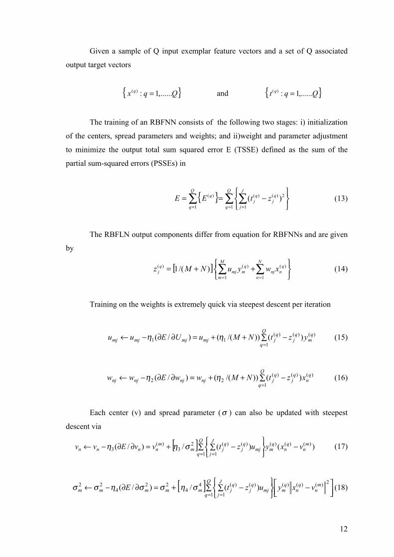
Given a sample of Q input exemplar feature vectors and a set of Q associated
output target vectors
{ }Qqx q ,......1:)( = and { }Qqt q ,......1:)( =
The training of an RBFNN consists of the following two stages: i) initialization
of the centers, spread parameters and weights; and ii)weight and parameter adjustment
to minimize the output total sum squared error E (TSSE) defined as the sum of the
partial sum-squared errors (PSSEs) in
{ }∑ ∑ ∑= = =
−==Q
q
Q
q
J
j
qj
qj
q ztEE1 1 1
2)()()( )( (13)
The RBFLN output components differ from equation for RBFNNs and are given
by
[ ]
++= ∑∑
==
N
n
qnnj
M
m
qmmj
qj xwyuNMz
1
)(
1
)()( )/(1 (14)
Training on the weights is extremely quick via steepest descent per iteration
)()(
1
)(11 )())/(()/( q
mq
j
Q
q
qjmjmjmjmj yztNMuUEuu −∑++=∂∂−←
=ηη (15)
)()(
1
)(22 )())/(()/( q
nq
j
Q
q
qjnjnjnjnj xztNMwwEww −∑++=∂∂−←
=ηη (16)
Each center (v) and spread parameter (σ ) can also be updated with steepest
descent via
[ ] )()(/)/( )()()(
1 1
)()(23
)(3
mn
qn
qm
Q
q
J
jmj
qj
qjm
mnnnn vxyuztvvEvv −∑
∑ −+=∂∂−←
= =σηη (17)
[ ]
−∑
∑ −+=∂∂−←
= =
2)()()(
1 1
)()(44
224
22 )(/)/( mn
qn
qm
Q
q
J
jmj
qj
qjmmmmm vxyuztE σησσησσ (18)

13
2.5 Responsive Perturbation Training
Responsive perturbation training (RPT) is a newly proposed [11] algorithm in
the traning arena. It uses the general philosophy of combining genetic algorithms (GA)
and simulated annealing (SA). Nonetheless, in RPT, both the GA and the SA are
changed in such a way that neither is the original optimization method other than the
slight semblance in the guidelines. For example, when a population is created,
individuals are not converted to binary strings, since no crossing occurs. Instead of
selecting the best performing individuals, only the best is kept.
Perturbation replaces the crossing. A new family of individuals are created by
perturbing the best solution. This guarantees that all the offsprings are the variations of
the best parent. The pertubation is a gaussian noise, whose variance is monotonically
decreasing or simply given by a function, added to the selected individual.
RPA is a simple and robust algorithm. Its simplicity saves on CPU time. Weight
and sigma update equations are given by
S (i,j) = S(i,j) + (percent error) * R,
w (i,j) = w(i,j) + (percent error) * R,
Where i=1...K, j=1...number of individuals, and
R = k * r. Here k is a suitable coefficient, less than unity, and r is Gaussian noise with
zero mean.
Thus RPA is an error-driven process. With the carefully arranged coefficient, weight
and spread parameters are perturbed less and less in amplitude by use of the error term.
This eliminates the occasional need for hill-climbing. Unless the error reaches a certain
level, the perturbation amplitude never drops and the algorithm keeps searching within a
specified search radius. At the outset, error is high and a rough search starts, and a
neighborhood of solution is sought to converge to. Once the neighborhood is roughly
spotted, the search closes in on the optimal vectors. Usually, towards the final stages of
the search, noise variance is reduced, and the coupled effect of error and the reduced
noise variance help smoothen the computed vectors.

14
Figure 2.6 Responsive Perturbation Algorithm [11].
2.6 How Does It Work?
Apart from the BP in RBFNN, every middle layer represents a cluster which has
a center in Gaussian distribution and they are represented by the mean (m) and cluster
diameter which is given by sigma (σ ). If we can represent the feature space with an
optimum number of clusters and appropriate sigma and mean, function can be more
easily approximated. And if the feature space can be sufficiently covered, systems
response will be improved.
However many nodes can be used at middle layer which means that more
clusters are used and it gives more accurate solutions, on the other hand operator should
avoid from over-fitting because it will not be a healthy solution.
And with the RBFLN algorithm additional links that combine the input nodes to
the output nodes also gives us a chance to cover the linear portion of the feature space.
It can easily be seen that the RBFNN needs cluster centers and we will see that
these centers can be initialized more accurately than a random process. A unsupervised
algorithm and a supervised algorithm are utilized to compliment them.
2.7 Clustering Algorithms
In a real world problem most of the time data must be arranged to make them
useful in applications where number of data is too many to calculate, most of the time
plenty of data is available, so their number must be decreased. Even in these conditions
a new datum must be classified correctly especially in pattern recognition application.

15
However as in the RBFNN, cluster centers must be known. With clustering algorithms
cluster centers can be found appropriately to cover the feature space.
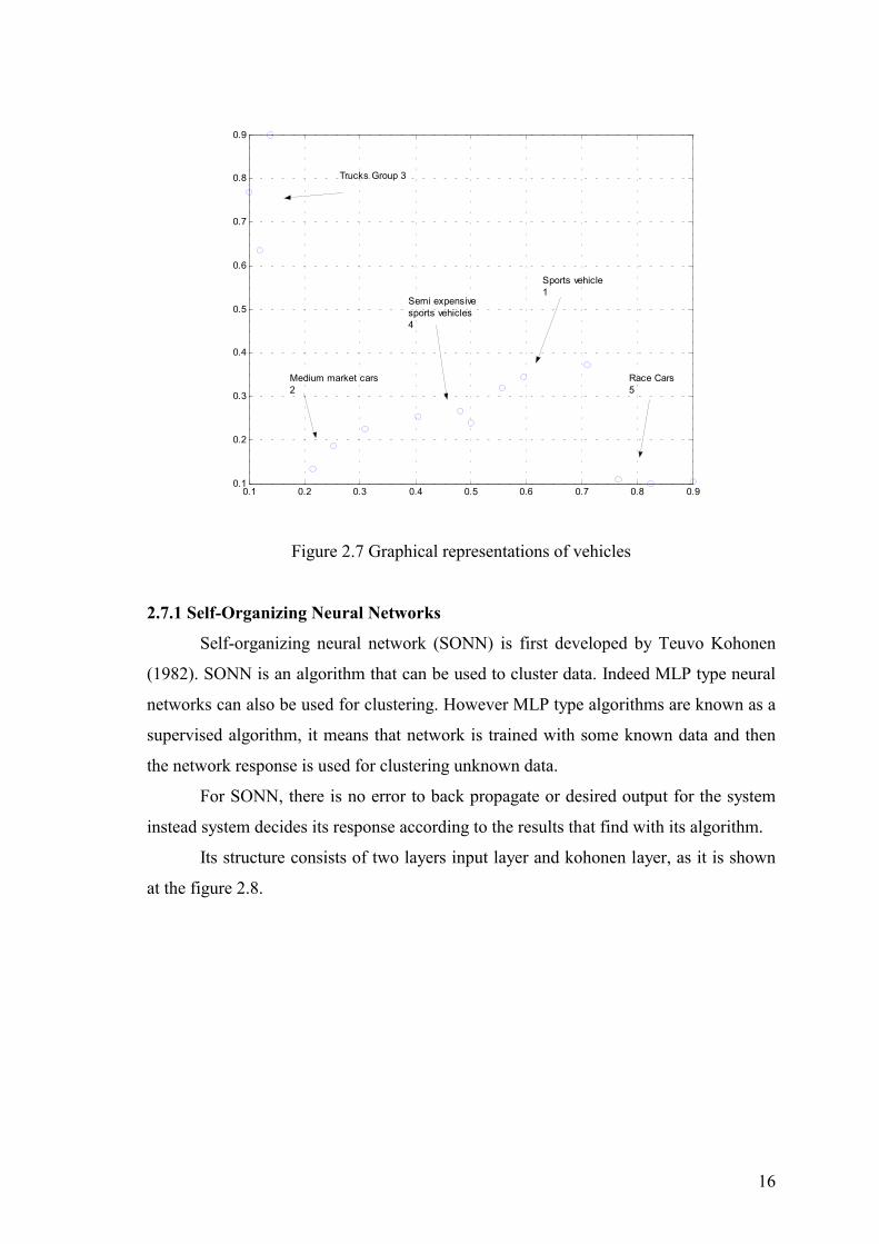
To visualize the clustering methods, following application will be introduced.
For the following data some vehicles are shown as a point in the figure 2.7 according to
their weight and speed.
As in the table 2.1, if a vehicle’s correct cluster is not known, at first sight it is
hard to recognize from the list of data. However if the data is drawn to a table it is more
easy to obtain the relation between these data.
Normalized data are used for this application to obtain more healthy solutions
and it is a good practice to use normalized data. In this application there are six clusters
sports vehicles, medium market cars, trucks, race cars, semi-expensive and sports
vehicles.
Instead of drawing a figure, an algorithm can be written to do this. In literature
there are some algorithms. In the following section these algorithms will be examined.
The author prefers k-means and SONN application to represent the supervised and
unsupervised algorithms respectively.
Table 2.1 Vehicle speed and weight information Experimental Data Sheet Normalized
Speed Weight Speed Weight
1 220 1300 Sports Vehicles 0.5571 0.3182
2 230 1400 0.5952 0.3446
3 260 1500 0.7095 0.3711
4 140 800
Medium Market
Cars 0.2524 0.1860
5 155 950 0.3095 0.2256
6 130 600 0.2143 0.1331
7 100 3000 Trucks 0.1000 0.7678
8 105 2500 0.1190 0.6355
9 110 3500 0.1381 0.9000
10 290 475 Race Cars 0.8238 0.1000
11 275 510 0.7667 0.1093
12 310 490 0.9000 0.1040
13 180 1050 Semi-expensive 0.4048 0.2521
14 200 1100 Sports Vehicles 0.4810 0.2653
15 205 1000 0.5000 0.2388
16
0.1 0.2 0.3 0.4 0.5 0.6 0.7 0.8 0.90.1
0.2
0.3
0.4
0.5
0.6
0.7
0.8
0.9
Trucks Group 3
Medium market cars 2
Semi expensivesports vehicles 4
Sports vehicle1
Race Cars5
Figure 2.7 Graphical representations of vehicles
2.7.1 Self-Organizing Neural Networks
Self-organizing neural network (SONN) is first developed by Teuvo Kohonen
(1982). SONN is an algorithm that can be used to cluster data. Indeed MLP type neural
networks can also be used for clustering. However MLP type algorithms are known as a
supervised algorithm, it means that network is trained with some known data and then
the network response is used for clustering unknown data.
For SONN, there is no error to back propagate or desired output for the system
instead system decides its response according to the results that find with its algorithm.
Its structure consists of two layers input layer and kohonen layer, as it is shown
at the figure 2.8.

17
Figure 2.8 Structure of SONN
Input layer is used to present the data. Kohonen layer nodes and their positions
represent the topological position of clusters and its link values can be assumed as their
center position.
Computation begins when the input data presented to the input layer. And every
input datum is compared with every kohonen layer node and their Euclidian distance is
calculated. After this calculation a winner node is found for each input datum as
follows.
Where )(,0 tn k : the thk node in the input layer at the time “t”. )(),(,1,0 tw yxk→
represents the link value which is combined to the thk node in the input layer from node
at kohonen layer which is placed at (x,y).
Algorithm of SONN is inspired from biology. In human brain there is a layer
which is called cerebral cortex. At cerebral cortex biological process depends on lateral
interaction like SONN. As in the figure 2.9 after calculation of the winning node,
winning node and its neighbors are updated. Nodes that are placed outside of this
boundary do not participate in learning.
∑=
→−=0
2))(),(,1,0)(,0()(,k
tyxkwtkntyxDist

Figure 2.9 Step functions that used to determine the nodes within the neighborhood
“N” term show
the width of the neig
increased. Learning
Neighborhood (H) an
the iteration.
Weight values
0 10 20 30 40 50 60 70 80 90 1000
0.2
0.4
0.6
0.8
1
1.2
NEIGHBOURHOOD
Participates in learning
Does not participate
W
(),(,1, tjiki → +∆
=
0
1
)(, tjiN
)()()()( tHtWinitHtin rowrow +≤≤−ia
Wf
nd)()()()( tHtWinitHtWin colcol +≤≤−
othervise18
s whether this node participates in learning or not. “H” represents
hborhood of the winning node and it is decreased as the time is
rate parameter (Lr) should be decreased appropriately.
d learning rate parameter should be minimum for the last 10% of
are updated according to the following procedure.
)1()()1( ),(,1,0,,0),(,1,0 +∆+=+ →→→ ttWt kikjikjik
))()1()(()1 ),(,1,0,0)1()1( twtntLrcolrowN jikitwintwin →++ −+=

2.7.2 K-Means Algorithm
K-means algorithm is a widely used clustering algorithm. Its strength comes
from its simple mathematical fundamentals, hence it can be easily implement able.
However k-means algorithm has supervised type and heuristic nature. So it must be
applied for many k terms.
Term “k” comes from the initialized number of clusters hence before running the
program, we know, how many clusters we are going to have. This procedure tries to
divide the feature space into number of “k” slices, according to the Euclidian distance
equation. Performance index for the ith cluster;
This algorithm is iterative k based on minimization of a performance index F.
K: Number of clusters specified by user.
F: Sum of squared distance of all points in a cluster to the cluster center.
1)
2) Each in
clusters acc
input datum
3) Update
cluster cent
4) If the ce
otherwise g
∑ ⋅==
iZxF
N
jiji
1
2
∑==
iFF
N
jii
1
{ }NXXX ,......., 21We have ınput data
{ }112
11 ,......., KZZZ
ClusX ∈
Choose initial cluster centers
N
dividual input datum classified into the one of the k number ofording to the distance between initial cluster centers and itself. And than the
is assigned to the cluster, which has minimum distance.
all cluster
ers should
nters are n
o to step 2
{ }iiX 1=
ter22 j
pj
m ZxZx −≤− ∀ mP ≠ )( j
iZ
M, ifcenters for i=1, 2 …K. Distance of all pa
be minimized.
ot changed for some number of iteration, iteratio
.
P, m=1, 2...K
19
tterns to the new
n can be stopped,
20
The k-means algorithm finds locally optimal solutions with respect to the
clustering error. It is a fast iterative algorithm that has been used in many clustering
applications. It is a point-based clustering method that starts with the cluster centers
initially placed at arbitrary positions and proceeds by moving the cluster centers at each
step in order to minimize the clustering error. The main disadvantage of the method lies
in its sensitivity to initial positions of the cluster centers. Therefore, in order to obtain
near optimal solutions using the k-means algorithm several runs must be done differing
in the initial positions of the cluster centers.
-1- It implies that the data clusters are ball-shaped because it performs
clustering based on the Euclidean distance.
-2-Also there is the dead-unit problem. That is, if some units are initialized far
away from the input data set in comparison with other units, they then immediately
become dead without learning chance any more in the whole learning process.
-3-It needs to pre-determine the cluster number. When k equals to optimum
number of k, the k-means algorithm can correctly find out the clustering centers.
Otherwise, it will lead to an incorrect clustering result, where some of centers do not
locate at the centers of the corresponding clusters. Instead, they are either at some
boundary points among different clusters or at points biased from some cluster centers.
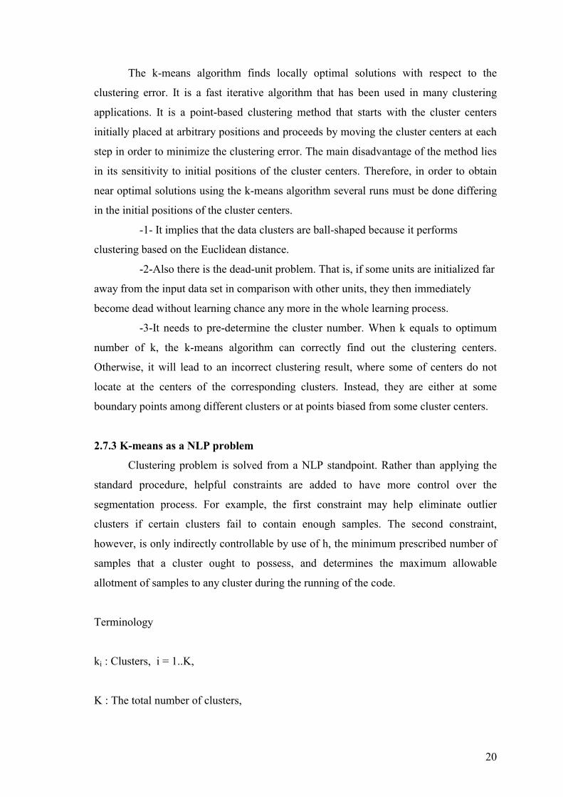
2.7.3 K-means as a NLP problem
Clustering problem is solved from a NLP standpoint. Rather than applying the
standard procedure, helpful constraints are added to have more control over the
segmentation process. For example, the first constraint may help eliminate outlier
clusters if certain clusters fail to contain enough samples. The second constraint,
however, is only indirectly controllable by use of h, the minimum prescribed number of
samples that a cluster ought to possess, and determines the maximum allowable
allotment of samples to any cluster during the running of the code.
Terminology
ki : Clusters, i = 1..K,
K : The total number of clusters,

21
h : The minimum number of data points required in a cluster to constitute a cluster.
N : The total number of data,
D : Data space, a dim x N matrix.
di : Vector of dimension dim, i = 1 .. N,
Pi : The number of data points in ith cluster, i = 1 ..K,
ci : ith cluster center of dimension dim, i = 1 .. K.
DkK
ii =
=Υ
1 (19)
∅=ji kk Ι , i j≠ (20)
-2- States that no fuzzy membership exists between the clusters and the clustering is, in
fact, a hard clustering.
DP ⊂⊆ ih (21)
N 2≥≥ K (22)
The Problem Statement;
Minimize Cost Function
J = )djci(1 1
2∑ ∑ −= =
K
i
N
j, kidj ∈ (23)
s.t.
i) hPi ≥ , where i = 1... K, (24)
and
22
ii)
∑ −−−≤
−
=
1
1r )()P(
i
ri hiKNP ,
Where i = 1... K. (25)
The constraint (24) enforces the lower limit in that the number of data within any cluster
may not be less than the prespecified h, and (25), given the data space, determines the
upper limit.
It should be noted that
∑ ==
K
ii NP
1 (26)
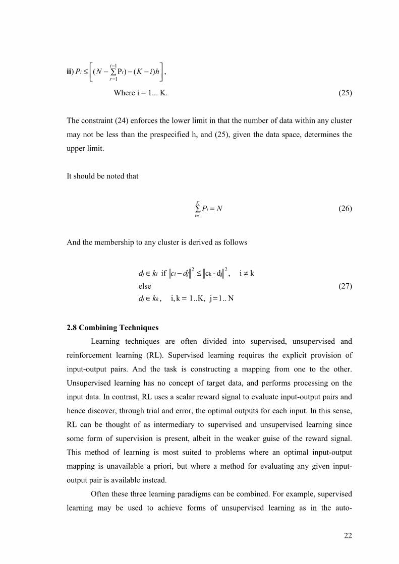
And the membership to any cluster is derived as follows
N .. 1 j ..K, 1 k i, ,else
ki ,d-c if
2jk
2
==∈
≠≤−∈
kj
jiij
kd
dckd (27)
2.8 Combining Techniques
Learning techniques are often divided into supervised, unsupervised and
reinforcement learning (RL). Supervised learning requires the explicit provision of
input-output pairs. And the task is constructing a mapping from one to the other.
Unsupervised learning has no concept of target data, and performs processing on the
input data. In contrast, RL uses a scalar reward signal to evaluate input-output pairs and
hence discover, through trial and error, the optimal outputs for each input. In this sense,
RL can be thought of as intermediary to supervised and unsupervised learning since
some form of supervision is present, albeit in the weaker guise of the reward signal.
This method of learning is most suited to problems where an optimal input-output
mapping is unavailable a priori, but where a method for evaluating any given input-
output pair is available instead.
Often these three learning paradigms can be combined. For example, supervised
learning may be used to achieve forms of unsupervised learning as in the auto-
23
associative MLP of [12]. Conversely, unsupervised learning can be used to support
supervised learning as, for example, in radial basis networks [13] and also the SOM-
MLP hybrid model of [14]. Alternatively, supervised learning can be embeded within an
RL framework. Examples are common, the Q-AHC algorithm of [15] (Based on the
adaptive heuristic critic (AHC) and actor-critic models of [16], [17], the backgammon
learning application of [18,19], the QCON arhitecture of [20], and the lift scheduler of
Crites and [21], all of which make use of the MLP and the backpropagation training
algorithm. Similarly, unsupervised learning may also be used to provide representation
and generalization within RL as in the self-organizing map (SOM) based approaches of
[22, 23].
In this research, radial basis function NN is used as a main function
approximator. In the process, it is crucial to cover the feature space. It is known that, to
cover the feature space radial basis cluster centers must be chosen appropriately. If the
centers can not be obtain appropriately computation time takes to long and most
probably the results will not be healthy.
To obtain the cluster centers the author prefers to use K-Means and SONN.
Additionally slight modifications are made on K-Means algorithm and also its
performance is compared.
2.8.1 SONN & RBFNN
When the SONNs are used, number of clusters that will be obtained at the end of
the process is not known or given initially. This is very useful for the process that the
system is searching through the unknown region. Sometimes our data base is very huge
and it needs to be diminished that can be used in process. Otherwise it needs huge time
to be processed.
It is much better when the cluster represented by a center and the cluster’s
diameter instead of great number of data point. This flexibility can be implemented
through the nature of RBFNN.
This algorithm will be discussed deeply at the simulations and experiments
section. However its simple architecture will be given in this section.
2.8.2 K-Means & RBFNN
In this combining techniques section, aim is to find the right cluster centers
appropriately and in the previous section unsupervised algorithm is used however in this
algorithm a supervised algorithm was used.

Both conventional K-means algorithm and the author modified K-means
algorithm need to be given initial number of cluster centers. Hence k-means algorithm
has a draw back. So, if the number of clusters can not be given appropriately, most
probably the solutions will be incorrect. Also this algorithm will be discussed in depth
at simulation and experiments' section.
SONN: to find the clusters and
Input dataFigure 2.10 Combined structures of SONN&RBFNN
Figu
their centers
RBFNN: to process the data
K-Means: to find the clusters and their centers
Input data24
re 2.11 Combined structures of K-Means & RBFNN
RBFNN: to process the data

25
CHAPTER 3
REINFORCEMENT LEARNING Reinforcement learning dates back to the early days of cybernetics and work in
statistics, psychology, neuroscience, and computer science. In the last five to ten years,
it has attracted increasing interest in the machine learning and artificial intelligence
communities. Its promise is beguiling a way of programming agents by reward and
punishment without needing to specify how the task is to be achieved. But there are
formidable computational obstacles to fulfilling the promise [24].
Reinforcement learning is the problem faced by an agent who must learn
behavior through trial-and-error interactions with a dynamic environment. The work
described here has a strong family resemblance to widely mentioned work in
psychology, but differs considerably in the details and in the use of the word
reinforcement." It is appropriately thought of as a class of problems, rather than as a set
of techniques.
There are two main strategies that are used in reinforcement problems. First is to
search the space to find the optimal solution, which is used in genetic algorithms and
some other novel search techniques. And the other is statistical and dynamic
programming methods. The author prefers to use these statistical methods. There is no
formally justified method.
In the following sections, some fundamental reinforcement lexicon will be
briefly discussed and then other crucial points will be given. For instance, should the
agent explore the environment? Or should it trust its previous knowledge? If the answer:
yes the agent should explore the environment and then there is another question. How
often should the agent explore. At this point trade off between exploration and
exploitation will be discussed.
To realize how a reinforcement learning agent behave or decide. TD (λ ) and Q-
Learning algorithms is going to be presented.

26
3.1 Reinforcement-Learning Model
In the standard reinforcement-learning model, an agent is connected to its
environment via perception and action, as depicted in Figure 3.1 [24] On each step of
interaction the agent Receives an input, i, and some indication of the current state, s, of
the environment; the agent then chooses an action, a, to generate as output. The action
changes the state of the environment, and the value of this state transition is
communicated to the agent through a scalar reinforcement signal, r. The agent's
behavior, B, should choose actions that tend to increase the long-run sum of values of
the reinforcement signal. It can learn to do this over time by systematic trial and error,
guided by a wide variety of algorithms that are the subject of later subsections of this
thesis.
Figure 3.1 Reinforcement agent and its interrreaction with environment
The model consists of
A discrete set of environment states, S;
A discrete set of agent actions, A; and
A set of scalar reinforcement signals; generally between {0, 1}, or the real numbers.
The figure 3.1 also includes an input function I, this parameter settle on how the agent
views the environment state; we will assume that it is the identity function. An intuitive
way to understand the relation between the agent and its environment is with the
following example dialogue [24].
Environment: You are in state 65. You have 4 possible actions.
Agent: I'll take action 2.

27
Environment: You received a reinforcement of 7 units. You are now in state 15. You
have 2 possible actions.
Agent: I'll take action 1.
Environment: You received a reinforcement of -4 units. You are now in state 65. You
have 4 possible actions.
Agent: I'll take action 2.
Environment: You received a reinforcement of 5 units. You are now in state 44. You
have 5 possible actions.
...
...
The agent's job is to find a policyπ , mapping states to actions, that maximizes some
long-run measure of reinforcement. We expect, in general, that the environment will be
non-deterministic; that is, that taking the same action in the same state on two different
occasions may result in different next states and/or different reinforcement values. This
happens in our example above: from state 65, applying action 2 produces differing
reinforcements and differing states on two occasions. However, we assume the
environment is stationary; that is, that the probabilities of making state transitions or
receiving specific reinforcement signals do not change over time.
Reinforcement learning differs from widely studied supervised learning
algorithm. In reinforcement learning there is no input/output pairs. Supervised
algorithms are trained to give the known solution for the known input, however in
reinforcement learning algorithm the agent tries to learn the optimum through the trial
and error sequences. It is the most important difference.
Reinforcement learning agent should be able to gather the appropriate data and
exploration and exploitation dilemma should be solved.
Some aspects of reinforcement learning are closely related to search and
planning issues in artificial intelligence. AI search algorithms generate a satisfactory
trajectory through a graph of states. Planning operates in a similar manner, but typically
within a construct with more complexity than a graph, in which states are represented by
compositions of logical expressions instead of atomic symbols. These AI algorithms are
less general than the reinforcement-learning methods, in that they require a predefined
model of state transitions, and with a few exceptions assume determinism. On the other
hand, reinforcement learning, at least in the kind of discrete cases for which theory has

28
been developed, assumes that the entire state space can be enumerated and stored in
memory an assumption to which conventional search algorithms are not tied.
3.2 Models of Optimal Behavior
To start the optimal behavior or learning algorithms, there is a question that
needs to be answered. What will be the optimality and how should the agent take into
account its future. And how should the agent decide about its actual action. In literature
there are three main methods to find the optimality.
The finite-horizon model is the easiest to think about; at a given moment in time,
the agent should optimize its expected reward for the next h steps:
∑
=
h
ttrE
0 (28)
there is no need to worry about what will happen after this sequence. In this and
subsequent expressions, tr represents the scalar reward received t steps through the
future. This model can be used in two ways. In the first, the agent will have a non-
stationary policy; that is, one that can change over time. On its first step it will take
what is termed an h-step optimal action. This is defined to be the best action available
given that it has h steps remaining in which to act and gain reinforcement. On the next
step it will take a (h-1)-step optimal action, and so on, until it finally takes a 1-step
optimal action and terminates. In the second, the agent does receding-horizon control, in
which it always takes the h-step optimal action. The agent always take action according
to the same policy, but the value of h limits how far ahead it looks in choosing its
actions. The finite-horizon model is not always suitable. In many cases we may not
know the precise length of the agent's life in real applications.
The infinite-horizon discounted model takes the long-run reward of the agent
into account, but rewards that are received in the future are geometrically discounted
according to discount factor, (where 10 <≤ γ ):
∑
∞
=0tt
t rE γ (29)
We can explain in several ways. It can be seen as an interest rate, a probability
of living another step, or as a mathematical trick to bind the infinite sum. The model is
conceptually similar to receding-horizon control, but the discounted model is more

29
mathematically tractable than the finite-horizon model. This is a main reason for the
wide attention this model has received.
Another optimality criterion is the average-reward model, in which the agent is
supposed to take actions that optimize its long-run average reward:
∑
=∞→
h
tth
rh
E0
1lim (30)
This method is called as a gain optimal policy; it can be seen as the limiting case
of the infinite-horizon discounted model as the discount factor approaches 1 [26].
Problem with this criterion is that there is no way to discriminate between two policies,
one of which gains a large amount of reward in the initial phases and the other of which
does not. Reward gained on any initial prefix of the agent's life is surpassed by the long-
run average performance. It is possible to generalize this model so that it takes into
account both the long run average and the amount of initial reward than can be gained.
In the generalized, bias optimal model, a policy is preferred if it maximizes the long-run
average and ties are broken by the initial extra reward. Figure 3.2 [24] contrasts these
models of optimality by providing an environment in which changing the model of
optimality changes the optimal policy. In this example, circles represent the states of the
environment and arrows are state transitions. There is only a single action choice from
every state except the start state, which is in the upper left and marked with an incoming
arrow. All rewards are zero except where marked. Under a finite-horizon model with h
= 5, the three actions yield rewards of +6.0, +0.0, and +0.0, so the first action should be
chosen; under an infinite-horizon discounted model with = 0.9, the three choices yield
+16.2, +59.0, and +58.5 so the second action should be chosen; and under the average
reward model, the third action should be chosen since it leads to an average reward of
+11. If we change h to 1000 and to 0.2, then the second action is optimal for the finite-
horizon model and the first for the infinite-horizon discounted model; however, the
average reward model will always prefer the best long-term average. Since the choice of
optimality model and parameters matters so much, it is important to choose it carefully
in any application.
The finite-horizon model is appropriate when the agent's lifetime is known; one
important aspect of this model is that as the length of the remaining lifetime decreases,
the agent's policy may change. A system with a hard deadline would be appropriately
modeled this way. The relative usefulness of infinite-horizon discounted and bias-

30
optimal models is still under debate. Bias-optimality has the advantage of not requiring
a discount parameter; however, algorithms for finding bias-optimal policies are not yet
as well-understood as those for finding optimal infinite-horizon discounted policies.
Figure 3.2 Comparing Models of Optimality. All unlabeled arrows produce a reward of
zero.
3.3 Exploitation versus Exploration
Main difference between reinforcement learning and supervised learning is that
a reinforcement-learner must explicitly explore its environment. In order to underline
the problems of exploration, we treat a very simple case in this section. The
fundamental issues and approaches described here will, in many cases, and can be used
to understand the more complex issues in the following chapters.
The simplest possible reinforcement-learning problem is known as the k-armed
bandit problem, which has been the subject of a great deal of study in the statistics and
applied mathematics literature [26]. The agent is in a room with a collection of k
gambling machines (each called a “one-armed bandit" in colloquial English). The agent
is permitted a fixed number of pulls, h. Any arm may be pulled on each turn. The
machines do not require a deposit to play; the only cost is in wasting a pull playing a
suboptimal machine. When arm i is pulled, machine i pays off 1 or 0, according to some
underlying probability parameter ip , where payoffs are independent events and the spi
are unknown. What should the agent's strategy be?
This problem illustrates the fundamental tradeoff between exploitation and
exploration. The agent might believe that a particular arm has a fairly high payoff
probability; should it choose that arm all the time, or should it choose another one that it
has less information about, but seems to be worse? Answers to these questions depend
on how long the agent is expected to play the game; the longer the game lasts, the worse
31
the consequences of prematurely converging on a sub-optimal arm, and the more the
agent should explore.
There is a wide variety of solutions to this problem. We will consider a
representative selection of them, but for a deeper discussion and a number of important
theoretical results, see the book by [26]. We use the term “action" to indicate the agent's
choice of arm to pull. This eases the transition into delayed reinforcement models.
3.4 Dynamic-Programming Approach
If the agent is going to be performing for a total of h steps, it can use basic
Bayesian analysis to solve for an optimal strategy [26]. This requires an assumed prior
joint distribution for the parameters{ }ip , the most natural of which is that each ip is
independently uniformly distributed between 0 and 1. We compute a mapping from
belief states to actions. Here, a belief state can be represented as a tabulation of action
choices and payoffs: { }kk wnwnwn ,.........,.........,,, 2211 denotes a state of play in which
each arm i has been pulled in times with iw payoffs. We write
( )kk wnwnwnV ,.........,.........,,, 2211* as the expected payoff remaining, given that a total
of h pulls are available, and we use the remaining pulls optimally.
If ∑ =i
i hn , then there are no remaining pulls, and. This is the basis of a recursive
definition. If we know the iw value for all belief states with t pulls remaining, we can
compute the *V value of any belief state with t + 1 pulls remaining:
( ) EikwknwnwnV max,.........,.........2,2,1,1* = (Future payoff if agent takes action i,
then acts optimally for remaining pulls)
Where ip is the posterior subjective probability of action i paying off given in , iw and
our prior probability. For the uniform priors, which result in a beta distribution,
ip = ( iw + 1) = ( in + 2).
The expense of filling in the table of *V values in this way for all attainable belief
states is linear in the number of belief states times actions, and thus exponential in the
horizon.
32
3.5 Delayed Reward
In reinforcement learning most of the case, the agent's actions determine not
only its immediate reward, but also the next state of the environment. These
environments can be thought of as networks of bandit problems, but the agent must take
into account the next state as well as the immediate reward when it decides which action
to take. In the long run the agent also determines the future rewards. The agent will have
to be able to learn from delayed reinforcement: it may take a long sequence of actions,
receiving unimportant reinforcement, and then finally arrive at a state with high
reinforcement. The agent must be able to learn which of its actions are desirable based
on reward that can take place arbitrarily far in the future.
3.6 Markov Decision Processes
For the delayed reinforcement modeling, Markov decision processes (MDPs)
can be used to describe. An MDP consists of
-a set of states S,
-a set of actions A,
-a reward function RASR →×: , and
-a state transition function )(: SAST ∏→× , where a member of )(S∏ is a probability
distribution over the set S (i.e. it maps states to probabilities). We write ),,( sasT ′ for
the probability of making a transition from state s to state s′ using action a. The state
transition function probabilistically specifies the next state of the environment as a
function of its current state and the agent's action. The reward function specifies
expected instantaneous reward as a function of the current state and action. The model is
Markov if the state transitions are independent of any previous environment states or
agent actions.
There are many good references to MDP models [27, 28, 29, and 30].
3.7 Finding a Policy Given a Model
Before searching algorithms for learning to move in MDP environments, we will
explore techniques for determining the optimal policy given a correct model. These
dynamic programming techniques will serve as the foundation and inspiration for the
learning algorithms to follow. We restrict our attention mainly to finding optimal
policies for the infinite-horizon discounted model, but most of these algorithms can be

33
assumed similar for the finite horizon and average-case models as well. We rely on the
result that, for the infinite-horizon discounted model, there exists an optimal
deterministic stationary policy [27].
We will speak of the optimal value of a state-it is the expected infinite
discounted sum of reward that the agent will gain if it starts in that state and executes
the optimal policy. Using π as a complete decision policy, it is written
∑=
∞
=0
* max)(t
ttrEsV γ
π (31)
The optimal value function is unique and can be defined as the solution to the
simultaneous equations
SssVsasTasREsVSsa
∈∀
∑ ′′+=
∈′,)(),,(),(max)( ** γ (32)
Which assert that the value of a state s is the expected instantaneous reward plus
the expected discounted value of the next state, using the best available action. Given
the optimal value function, we can specify the optimal policy as
∑ ′′+=
∈′ SsasVsasTasRs )(),,(),(maxarg)( ** γπ (33)
3.8 Learning an Optimal Policy
In the previous section we reviewed methods for obtaining an optimal policy for
an MDP assuming that we already had a model. The model consists of knowledge of the
state transition probability function ),,( sasT ′ and the reinforcement function R(s,a).
Reinforcement learning is primarily concerned with how to obtain the optimal policy
when such a model is not known in advance. The agent must interact with its
environment directly to obtain information which, by means of an appropriate
algorithm, can be processed to produce an optimal policy.
At this point, there are two ways to proceed.
-Model-free: Learn a controller without learning a model.
- Model-based: Learn a model, and use it to derive a controller.
Which approach is better? This is a matter of some debate in the reinforcement-learning
community. A number of algorithms have been proposed on both sides. This question

34
also appears in other fields, such as adaptive control, where the dichotomy is between
direct and indirect adaptive control.
The biggest problem facing a reinforcement-learning agent is temporal credit
assignment. How do we know whether the action just taken is a good one, when it might
have far reaching effects? One strategy is to wait until the “end" and reward the actions
taken if the result was good and punish them if the result was bad. In ongoing tasks, it is
difficult to know what the “end" is, and this might require a great deal of memory.
Instead, we will use insights from value iteration to adjust the estimated value of a state
based on the immediate reward and the estimated value of the next state. This class of
algorithms is known as temporal difference methods [31]. We will consider two
different temporal-difference learning strategies for the discounted infinite-horizon
model.
3.9 TEMPORAL DIFFERENCE LEARNING So far, some neural network and classification methods are discussed. These
methods can be assumed as prediction methods. For instance, classification methods
predict the cluster of the unknown data. Also conventional neural network methods
predict the output for unknown input according to the known input output pairs. These
methods assign credits by means of the difference between actual output and the
predicted output. Temporal Difference Learning methods assign credits by means of the
temporally successive predictions. Although such temporal difference methods have
been used in samuel’s checker player, Holland’s bucket brigade and in the Adaptive
Heuristic Critic. The author prefers to use TD methods because it requires less memory
and less computational time than conventional methods and it gives better results for
real world problems. In literature there are some real world applications show that TD
methods deserve to be investigated and used in real engineering and robotics problems.
Especially [17] applied the TD method to Backgammon and obtains the world master
level backgammon player computer software.
This research purpose is to create an autonomous agent that is capable to learn
from its past experience. After having built this kind a system, there is no need to know
the output that should be instead it is enough to gather sensory inputs from the
environment and let the agent learn its optimal behavior. Fro instance, agent should
predict whether this formation will led to win or end up with loss or from the cloud

35
formation it can be capable to predict whether it is going to be rain or not. For particular
economic condition whether the stock market will rise [32].
Apart from conventional learning algorithm credit assignment is made by
means of the difference between temporary successive predictions, whether there is a
change between the predictions over time. For example, suppose a weatherman attempts
to predict on each day of the week whether it will rain on the following Saturday. The
conventional approach is to compare each prediction to the actual outcome whether or
not it does rain on Saturday. A TD approach, on the other hand, is to compare each day's
prediction with that made on the following day. If a 50% chance of rain is predicted on
Monday, and a 75% chance on Tuesday, then a TD method increases predictions for
days similar to Monday, whereas a conventional method might either increase or
decrease them depending on Saturday's actual outcome.
TD methods have two kinds of advantages over conventional prediction
learning methods. First, they are more incremental and therefore easier to compute. For
example, the TD method for predicting Saturday's weather can update each day's
prediction on the following day, whereas the conventional method must wait until
Saturday, and then make the changes for all days of the week. The conventional method
would have to do more computing at one time than the TD method and would require
more storage during the week. The second advantage of TD methods is that they tend to
make more efficient use of their experience: they converge faster and produce better
predictions. We argue that the predictions of TD methods are both more accurate and
easier to compute than those of conventional methods.
The earliest and best-known use of a TD method was in [33] celebrated checker-
playing program. For each pair of successive game positions, the program used the
difference between the evaluations assigned to the two positions to modify the earlier
one's evaluation. Similar methods have been used in [34] bucket brigade, in Adaptive
Heuristic Critic [16, 17], and in learning systems studied by [35, 36, 37]. TD methods
have also been proposed as models of classical conditioning [38, 39, 40, 41, and 42].
Although TD prediction method is applied successfully, TD method can not be
understood theoretically, most probably because it is being used in complex problems.
In these systems TD employed as a better evaluation function predictor.
The TD method explanation is focused on numerical prediction processes rather
than on rule-based or symbolic prediction. The approach taken here is much like that

36
used in connectionism and in Samuel's original work our predictions are based on
numerical features combined using adjustable parameters or "weights."
This research uses TD methods with conventional methods in some simple
application to compare their performance. TD methods presented here can be directly
extended to multilayer networks.
3.9.1 TEMPORAL DIFFERENCE AND SUPERVISED METHODS IN
PREDICTION POBLEMS
Supervised learning techniques are known as the most important and widely
used learning paradigms. Supervised learning methods try to approximate the relation
between input and output pairs. After learning takes place, when the input presented, the
system responds it according to this relation. This paradigm has been used in pattern
classification, concept acquisition, learning from examples, system identification, and
associative memory. For example, in pattern classification and concept acquisition, the
first item is an instance of some pattern or concept, and the second item is the name of
that concept. In system identification, the learner must reproduce the input-output
behavior of some unknown system. Here, the first item of each pair is an input and the
second is the corresponding output.
Supervised learning methods can be applied any type of learning
algorithms. If the pair wise tabulation of the used data can be obtained, the supervised
algorithm can be trained. For whether forecasting one can gather data for Monday
prediction as input and Saturday actual output as the target value to predict the
Saturday’s whether in the same way Tuesday and Wednesday’s data can be trained
according to the actual output of the Saturday. It is easy to understand and analyze. It is
called supervised prediction method and it is widely used. However it is not preferable
and this type of prediction method is not appropriate for this kind of problem.
3.9.2 SINGLE STEP AND MULTI-STEP PREDICTION
In TD methods there are two types of prediction methods; one of them is the
single step prediction and the other one is called the multi-step prediction problem. In
single step prediction correctness of the prediction will be given at each step. In multi-
step prediction the correctness of the prediction is not revealed until more then one step
takes place, however partial information is revealed at each step. For example, the
weather prediction problem mentioned above is a multi-step prediction problem because

37
inconclusive evidence relevant to the correctness of Monday's prediction becomes
available in the form of new observations on Tuesday, Wednesday, Thursday and
Friday. On the other hand, if each day's weather were to be predicted on the basis of the
previous day's observations that is, on Monday predict Tuesday's weather, on Tuesday
predict Wednesday's weather, etc. one would have a single-step prediction problem,
assuming no further observations were made between the time of each day's prediction
and its confirmation or denial on the following day.
In single step application it is not possible to distinguish the difference from
supervised algorithm. Hence the advantage of the TD learning paradigm can be obtained
in multi step prediction problem. For example, predictions about next year's economic
performance are not confirmed or disconfirmed all at once, but rather bit by bit as the
economic situation is observed through the year. The likely outcome of elections is
updated with each new poll, and the likely outcome of a chess game is updated with
each move.
In real world many single step prediction can be thought as multi step prediction.
For pattern recognition problem mostly supervised algorithms are used with known
correctly classified pair of data. However when human sees something, he or she has a
concept about the object that is seen and after each perception this concept is updated
with the information that gives us a capability to update.
3.9.3 Computational issues
In this section some practical issues is going to be discussed with the theoretical
issues. During this section TD family of learning will be discussed on the basis of
supervised learning procedure. Mostly on Widrow-Hoff learning rule as it was
discussed. And then other different TD learning procedures will be introduced.
We consider multi-step prediction problems in which experience comes in
observation-outcome sequences of the form zxxxx m ,,.....,, 321 where each tx is a vector
of observations available at time t in the sequence, and z is the outcome of the sequence.
Many such sequences will normally be experienced. The components of each tx are
assumed to be real-valued measurements or features, and z is assumed to be a real-
valued scalar. For each observation outcome sequence, the learner produces a
corresponding sequence of predictions ,,.....,, 321 mPPPP each of which is an estimate of
z. In general, each tP can be a function of all preceding observation vectors up through

38
time t, but, for simplicity, here we assume that it is a function only of tx . The
predictions are also based on a vector of modifiable parameters or weights, w. tP 's
functional dependence on tx and w will sometimes be denoted explicitly by writing it as
),( wxP t .
Learning can be described as the update procedure of the w. In TD learning
weights are updated after a sequence completed and a terminal state is reached. Not
after each observation.
∑∆+==
m
ttwww
1 (34)
This procedure can be cast into more or less incremental phases. One can update
the weights after each observation or all the sequences completed.
Supervised learning algorithm considers the input and output as
pairs ),(),........,(),,( 21 zxzxzx m . The increment in weights depends on the difference
between tP and z, as the time progresses. The supervised learning formulation can be
given as in the following form.
,)( twtt PPzw ∇−=∆ α (35)
α term stand for the learning parameter and effect the learning. twP∇ term
stands for the partial derivative of the term tP with respect to each component of w.
For example, consider the special case in which tP is a linear function of tx and
w, that is, in which ∑== i ttT
t ixiwxwP )()( , where w(i) and )(ixt are the i'th
components of w and tx , respectively. In this case we have ,ttw xP =∇ and the
formulation reduces to the well known Widrow-Hoff rule [1]:
,)( ttT
t xxwzw −=∆ α (36)
This linear learning method is also known as the "delta rule," the ADALINE,
and the LMS filter. It is widely used in connectionism, pattern recognition, signal
processing, and adaptive control. The basic idea is that the difference
txTwz − represents the scalar error between the prediction, txTw , and what it should
have been, z. This is multiplied by the observation vector tx to determine the weight
changes because tx indicates how changing each weight will affect the error. For

39
example, if the error is positive and )(itx is positive, then )(tiw will be increased,
increasing tT xw and reducing the error. The Widrow-Hoff rule is simple, effective, and
robust.
Having being given formulation is for the one layer problems generalization has
already been made in Backpropagation procedure. In this case tP is solved in multilayer
structure as a nonlinear case. However, only difference is the way to solve the partial
differential of the gradient twP∇ .
In these equations there is a disadvantage, tw∆ depends on the final outcome z. It
means that all the formation until the final sate must be stored and the sequential process
is not allowed.
However in TD methods this process can be changed into incremental procedure
by the change; if tPz − assumed as the sum of all predictions.
∑ −=−=
+m
tkkkt PPPz )( 1 (37)
Hence the fallowing formulation can be obtained;
∑ ∇−∑+=∑ ∇−+==
+==
m
tktwkk
m
t
m
ttwt PPPwPPzww )()( 1
11αα (38)
∑ ∇−∑+==
+=
k
tktwkk
m
tPPPw )( 1
1α
∑∇−∑+==
+=
t
kkwtt
m
tPPPw
11
1)(α
At the end converting to the equation (34);
∑∇−=∆=
+t
kkwttt PPPw
11 )(α (39)
Unlike (38), this equation can be computed incrementally, because each tw∆
depends only on a pair of successive predictions and on the sum of all past values
for twP∇ . This saves substantially on memory, because it is no longer necessary to
individually remember all past values of twP∇ . Equation (39) also makes much milder
demands on the computational speed of the device that implements it; although it
requires slightly more arithmetic operations overall (the additional ones are those
needed to accumulate ∑ ∇=tk kwP1 ), they can be distributed over time more evenly.
Whereas (39) computes one increment to w on each time step, (38) must wait until a

40
sequence is completed and then compute all of the increments due to that sequence. If M
is the maximum possible length of a sequence, then under many circumstances (39) will
require only 1/Mth of the memory and speed required by (38).
Equation (39) is called TD (1) procedure. This type of learning algorithms are
called )(λTD procedure and this will be investigated in the following section.
3.9.4 )(λTD Learning procedures
Influence of TD learning procedure comes from its sensitivity of to the changes
between successive predictions. However supervised algorithms are sensitive to the
changes between the predictions and the final outcome. When there is a change occurs
between tP and 1+tP then it effects the changes on weights tw∆ . These changes predict
the difference between the all input data or the some portions of the previous inputs.
When the equation (39) is applied to a prediction problem, all the predictions are
affected equally. However for some reasons when latest predictions make more
alternation on the system, this will give more correct solution. It can be obtained by the
following formulations. In which alterations to the predictions of observation vectors
occurring k steps in the past are weighted according to kλ for 10 ≤≤ λ :
∑ ∇−=∆=
−+
t
kkw
ktttt PPPw
11 )( λα (40)
For λ =1 equation (40) will be equal to the equation (39). And this procedure is
called as the TD (λ ) algorithms. Hence the equation (39) called as TD (1).
Change of past predictions can be weighted in ways other than the exponential
form given above, and this may be appropriate for particular applications. However, an
important advantage to the exponential form is that it can be computed incrementally.
Given that te is the value of the sum in (40) for t, we can incrementally compute te + 1,
using only current information.
∑ ∇=+
=
−++
1
1
11
t
Kkw
ktt Pe λ
∑ ∇+∇==
−++
t
Kkw
kttw PP
1
11 λ
ttw eP λ+∇= +1

41
When the term λ is chosen less then 1, the learning procedure weight changes
differ from any supervised learning. And this difference reaches its maximum point
when the term λ is chosen as 0. If the term λ equals to the 0, it means that weight
changes affected by the most recent changes.
twttt PPPw ∇−=∆ + )( 1α
With these calculations, supervised learning algorithm is obtained with a little
difference. The term z, which is final outcome, is replaced by the term 1+tP . This shows
that supervised learning mechanism is the same when the λ term is chosen as 0.
3.9.5 )(λTD Learning procedures outperforms supervised scheme?
In literature there are some examples that show TD learning scheme outperforms
supervised algorithms. However there is an intuitive denial, because in supervised
learning the final outcome is known and the predictions are updated according to this
actual information. On the other hand TD learning procedure tries to minimize the
temporal difference. With this scheme one can converge more rapidly and accurately in
dynamic world problems, which is ubiquitous. Almost any real system is a dynamical
system, including the weather, national economies, and chess games. In this section, we
develop two illustrative examples: a game-playing example to help develop intuitions,
and a random-walk example as a simple demonstration with experimental results.
3.9.6 A Game Playing Example
Game playing consists of sequences of positions. Some of them is lead our game
to win while others lead to loss. This can be backgammon or one of the card games. For
example there is a state that we know that with 90% probability it leads to loss but with
only 10% probability leads to win. However after a novel game formation this “bad”
game condition is played and it leads us to win. How one can assign the credits to these
game positions. This situation is showed at the figure 3.3.

42
Figure 3.3 A novel game position that can reach win or loss.
Classical supervised learning procedure assigns the credits according to the final
outcome however this will affect the novel position as well. However TD methods
assign credits according to the temporal difference between successive predictions.
Indeed there is a disadvantage that in this example, we have ignored the possibility that
the bad state's previously learned evaluation is in error. Such errors will inevitably exist
and will affect the efficiency of TD methods in ways that cannot easily be evaluated in
an example of this sort. The example does not prove TD methods will be better on
balance, but it does demonstrate that a subsequent prediction can easily be a better
performance standard than the actual outcome.
This game-playing example can also be used to show how TD methods can fail.
Suppose the bad state is usually followed by defeats except when it is preceded by the
novel state, in which case it always leads to a victory. In this odd case, TD methods
could not perform better and might perform worse than supervised-learning methods.
Although there are several techniques for eliminating or minimizing this sort of
problem, it remains a greater difficulty for TD methods than it does for supervised-
learning methods. TD methods try to take advantage of the information provided by the
temporal sequence of states, whereas supervised-learning methods ignore it. It is
possible for this information to be misleading, but more often it should be helpful.

43
3.9.7 A Random Walk Example
So far TD methods discussed in a relatively complex way, however to make
clear the definition and to pave the way to theoretical results the notion of the TD
learning must be understood. In the following section there is an example which can be
also used to identify the nature of the Markov decision process. In the following
example which is called Bounded Random Walks.
In the bounded random walks, agent can choose an action to move right or left.
Game is terminated when the agent reaches to the one of the terminal state. This play
ground is shown in the figure 3.4.
Figure 3.4 Random walk example.
Terminal states are the right most or the left most states in which “G” or “A”
respectively. Every game starts from the state “D”. If either edge state (A or G) is
entered, the walk terminates. A typical walk might be DCDEFG. Suppose we wish to
estimate the probabilities of a walk ending in the rightmost state, G, given that it is in
each of the other states.
When the linear supervised learning scheme is used, and the final outcome given
when the system reaches to the state A z=0, if reaches to the state G z=1. The learning
methods estimated the expected value of z; for this choice of z, its expected value is
equal to the probability of a right-side termination. For each non-terminal state i, there
was a corresponding observation vector ix ; if the walk was in state i at time t
then ixtx = . Thus, if the walk DCDEFG occurred, then the learning procedure would be
given the sequence XD, XC, XD, XE, X F, 1. The vectors { }ix were the unit basis
vectors of length 5, that is, four of their components were 0 and the fifth was 1 (e.g., XD
=(0,0,1,0,0)T), with the one appearing at a different component for each state. Thus, if
the state the walk was in at time t has its 1 at the ith component of its observation
vector, then the prediction tT
t xwP = was simply the value of the ith component of w.
We use this particularly simple case to make this example as clear as possible. The

44
theorems we prove later for a more general class of dynamical systems require only that
the set of observation vectors { }ix be linearly independent.
3.9.8 Theoretical Approach to the TD Learning
So far, TD learning procedure has been discussed in a more heuristic way.
However to understand the way it works and how it works, some theoretical notions
need to be developed also to make further development more scientific approach is
needed. In the following section this theoretical approach will be developed. The theory
developed here relate to the linear TD (0) procedure and a class of tasks characterized
by the random walk example discussed in the previous section. Two major results are
presented: 1) an asymptotic convergence theorem for linear TD (0) when presented with
new data sequences; and 2) a theorem that linear TD (0) converges under repeated
presentations to the optimal estimates. Finally, how TD methods can be viewed as
gradient-descent procedures. 3.9.10 TD (0) Learning
Through this section process is assumed as a Markov decision process, in which
next state depends only on the current state. The states are defined as in the following
form, T stands for the terminal states and N stands for the non-terminal states. The term
ijP stands for the probability of transition from state i to state j. In which the agent
stands at state i, ),( TNjNi ∪∈∈ . The "absorbing" property means that indefinite
cycles among the non-terminal states are not possible; all sequences except for a set of
zero probability eventually terminate. Given an initial state 1q , an absorbing Markov
process provides a way of generating a state sequence 1,.......321 ,, +mqqqq ,
where Tmq ∈+1 . the initial state is chosen probabilistically from among the non-
terminal states will be assumed, each with probability iµ . As in the random walk
example, the learning algorithms direct knowledge of the state sequence will not be
given, but only of a related observation-outcome sequence zxxxx m ,,, ,......321 . Each
numerical observation vector tx is chosen dependent only on the corresponding non-
terminal state tq , and the scalar outcome z is chosen dependent only on the terminal
state 1+mq . In what follows, we assume that there is a specific observation vector ix

45
corresponding to each non-terminal state i such that if iqt = , then it xx = . For each non-
terminal state j, we assume outcomes z are selected from an arbitrary probability
distribution with expected value jZ .
To go forward for this section, it needs to be proved that this learning scheme
converges asymptotically. This problem can be cast into map the input states ix s into
the final outcome z. That is, we want the predictions ),( wixP to equal { }izE | , Ni ∈∀ .
Let us call these the ideal predictions. Given complete knowledge of the Markov
process, they can be computed as follows:
{ } ∑∈
∑∈
∑∈
++∑∈
∑∈
∑∈
+=Nj Nk Tl
lzklpjkpijpTj Nj Tk
kzjkpijpjzijpizE ......| (41)
For any matrix M, let [ ]ijM denote its ij'th component, and, for any vector v, let
[ ]iv denote its i'th component. Let Q denote the matrix with entries [ ] ijpijQ =
for Nij ∈ , and let h denote the vector with components [ ] ∑ ∈= Tj jzijpih for Ni ∈ .
Then we can write the above equation as
{ }i
hQIik
hkQizE
−−=
∑∞
== 1
0| (42)
kQ is the probabilities of going from one non-terminal state to another in k
Steps; for an absorbing Markov process, these probabilities must all converge to 0 as
∞→k .
For any absorbing Markov chain, for any distribution of starting probabilities iµ ,
for any outcome distributions with finite expected values jz , and for any linearly
independent set of observation vectors{ }Niix ∈| , there exists an 0>ε such that, for all
positive a < e εα < and for any initial weight vector, the predictions of linear TD (0)
(with weight updates after each sequence) converge in expected value to the ideal
predictions . That is, if nw denotes the weight vector after n sequences have been
experienced, then

46
{ } { } Nii
hQIizEnwTixEn ∈∀
−−==∞→ ,1|lim
PROOF: Linear TD (0) updates nw after each sequence as follows, where m denotes the
number of observation vectors in the sequence:
∑=
∇−++=+m
ttPwtPtPnwnw
1)1(1 α
∑−
=∇−+∇−++=+
1
1)()1(1
m
tmPwmPztPwtPtPnwnw αα
∑−
=−+−++=+
1
1)()1(1
m
tmqxmqxT
nwztqxtqxTnwtqxT
nwnwnw αα
Wheretqx is the observation vector corresponding to the state tq entered at time
t within the sequence. This equation allows us to separate the system into transition
from initial state to the next state.
∑∈
∑∈
−+−+=+Ni Nj
ixixTnwzijnixixT
nwjxTnwijnnwnw )()(1 αα
Where ijn denotes the number of times the transition ji → occurs in the
Sequence. (For Tj ∈ , all but one of the ijn is 0.)
In this process random number generator is used hence the actions that is taken
by agent are independent o each other. Expected value of each state can be calculated as
in the following form.
{ } ∑∈
∑∈
−+∑∈
∑∈
−+=+Ni Tj
ixixTnwjzijPid
Ni TjixixT
nwjxTnwijPidnwnwnwE )()(|1 αα
Where id is the expected number of times the Markov chain is in state i in one
sequence, so that iji pd is the expected value of ijn .
1)( −−= QITTd µ
Where [ ] idid = and [ ] ii µµ = , Ni ∈ . Each id is strictly positive, because any
state for which 0=id has no probability of being visited and can be discarded. Let nw

47
denote the expected value of nw . Then, since the dependence of { }nn wwE |1+ on nw is
linear, we can write
∑∈
∑∈
∑∈
∑∈
−+−+=+Ni Nj Ni Tj
ixixTnwjzijpidixixT
nwjxTnwijpidnwnw )()(1 αα
an iterative update formula in nw that depends only on initial conditions. Now we
rearrange terms and convert to matrix and vector notation, letting D denote the diagonal
matrix with diagonal entries [ ] iii dD = and X denote the matrix with columns ix .
)(1 ∑∪∈
−∑∈
∑∈
+∑∈
+=+TNj
ijpixTnw
Nj NjTnwijpjzijp
Niixidnwnw α
[ ] )(1 ∑∈
−+∑∈
+=+Nj
ixTnwjxT
nwijphNi
ixidnwnw α
)( nwTXnwTQXhXDnw −++= α
)(1 nwTXnwTQXhXDTXnwTXnwTX −++=+ α
nTT wXQIXDQXIXDh )(( −−+=α
0))((1
0))(( wTXnQIXDTXIDh
n
kXTXkQIXDTXI −−+∑
−
=−− ααα
when the following equation is assumed 0))((lim =−−→∞nQIXDTXIn α and
the following theorem is true, if 0lim =∞→n
n A , then I-A has an inverse, and
∑∞==−− 0
1)( iiAAI . Equations converge to
XDhTXQIXDTXIInwTXn
αα 1)))(((lim −−−−=∞→
XDhTXXTXDQI αα 11)(11)( −−−−−=

48
hQI 1)( −−=
{ } Nii
hQInwTixE
n∈∀
−−=
∞→,1)(lim
This is the desired result. Note that 1−D must exist because D is diagonal with
all positive diagonal entries, and 1)( −XX T must exist.
It thus remains to show that 0))((lim =−−∞→nQIXDTXIn α . We do this by
first showing that D (I-Q) is positive definite, and then that )( QIXDX T − has a full set
of eigen values all of whose real parts are positive. This will enable us to show that a
can be chosen such that all eigen values of )( QIXDXI T −−α are less than 1 in
modulus, which assures us that its powers converge.
3.9.11 Gradient Descent in TD Learning Gradient descent learning method is widely used in MLP. This method
guaranties to converge if the learning rate chosen small enough and the number of
iteration is suffice to converge. Gradient descent method is also called as hill climbing
method. Which is tries to minimize the overall error j (w). In this method gradient of the
overall error is calculated and the system’s weights tuned through the opposite direction.
This can be formalized as follows.
)( twjwtw ∇−=∆ α
Where the term α represents the learning rate and gives us the step size for the hill
climbing.
For the multi step prediction problem, system tries to approximate the term
),( wxpp tt = to the term { }txzE | and the error can be calculated by the difference
between target value and the prediction’s Euclidian distance.
{ }( ){ }2),(|)( wxpxzExEwj −=

49
where Ex{ } denotes the expectation operator over observation vectors x. J(w)
measures the error for a weight vector averaged over all observation vectors, but at each
time step one usually obtains additional information about only a single observation
vector. The usual next step, therefore, is to define a per-observation error measure
Q(w,x) with the property that { } )(),( wjxwQEx = . For a multi-step prediction problem,
{ }( )2),(|),( wxpxzExwQ −=
To determine the each step’s increment gradient of the each error is computed as
following ),( txwQw∇ , and if the following equation is assumed
correct { } )(),( wjwxwQwxE ∇=∇ . Weight update rule becomes as follows;
),( txwQwtw ∇−=∆ α
{ }( ) ),(),(|2 wtxpwwtxptxzE ∇−= α
In this prediction problem { }txzE | is not known or predicted initially. One can
use supervised learning methods to predict the expected value. In this case { }txzE | is
matched to the actual outcome z. On the other hand if the TD method is used { }txzE | is
matched to the next state prediction ),1( wtxp + . In the last case the TD (0) prediction
method is obtained, in which every prediction approximate to the subsequent prediction.
3.10 Q-Learning
Q-learning was first developed by Watkins [44, 45]. Q-learning is relatively
simple and easy to implement. Because of these specifications, it is widely used. If
),(* asQ is the discounted expected value of the taking action a in state s. Note that
)(* sV is the value of s assuming the best action is taken initially, and so
),(max)( ** asQsV a= . ),(* asQ can hence be written recursively as
∑ ′′′+=′′
),(*max),,(),(),(*asQsasTasRasQ
a
γ

50
Note also that, since ),(*max)(* asQasV = , we have ),(maxarg)( * asQs a=π
as an optimal policy.
Q-learning procedure can be cast into iterative form. At each step agent takes the
action which has maximum Q value. These values are stored in tabular form. And if
each state visited infinitely, while the term α is decayed appropriately. Q values
approximate the optimal value with probability 1 [44, 46, and 47].
After the Q values approximate to the optimal values, greedy action selection
method can be used. In literature, there is no formally justified method for the
exploration & exploitation dilemma.
3.11 Problem Description The problem is to build a system which can interact with its environment, and
learns from its past experience in dynamically changing conditions. To achieve this
task, system must be capable of learn in trial and error sequence. However how can the
system know that its action is reasonable or optimal in that condition? To test whether
the chosen action leads to win or lose, a utility must be assigned to tell the system it is
improving itself or it has to try something else. In the figure 3.1 a solution to this
problem is proposed by [46]. This system can be improved by adding extra networks.
Figure 3.1 Framework for connectionist Q-learning.
In the figure 3.1 connectionist Q-learning is given as an example. And in the
following its algorithm is given as a pseudo code.
1. x← current state; for each action ),(, ixutilUi i ←
2. a ← select(U,T);
3. Perform action a; (y;r) ←new state and reinforcement;

51
4. { }actionskkyutilru ∈+←′ |),(maxγ
5. Adjust utility network by backpropagating error U∆
through it with input x, where −′
=∆0
UuUi
6. Go to 1.
Generally speaking, the utility of an action a in response to a state x is equal to
the immediate payoff r plus the best utility that can be obtained from the next state y,
discounted by γ Therefore, the desired util function must satisfy
{ }actionskkyutilru ∈+←′ |),(maxγ
If i=a otherwise
52
CHAPTER 4
EXPERIMENTS So far supervised, unsupervised and reinforcement learning algorithms are
discussed. During the preparation of this thesis many applications are made. In this
chapter, these experiments and their results will be discussed.
Neural network applications are all written in C++ ID environment. Their
interface samples are given at appendix A.
4.1 Simulation for Combined Techniques Two combinations were simulated. First SON and RBFLN with gradient descent
training, and secondly K-means and RBFNN with RP training. The simulation data are
obtained from [24] and in appendix B. For RPT, case 1, R is 0.15 and R is reduced by
an amount of 0.01 every 10% of the running of the code. For case 2, again R is taken
0.15, and reduced by 25% after the first half of the training, and in the last tenth of the
running, it is reduced by 90%. RP training was run for 5000 epochs for both cases, and
the rate of acceptance based on the fitness is about half for the first case and one third
for the latter.
In this study, two novel ideas have been presented. K-means clustering is
formulated as a NLP, and by specific constraints, outlier clustering was eliminated.
Once a minimum number of samples to be contained in a cluster was specified, no such
cluster is allowed below that certain limit.
And finally, a new heuristic training is proffered. Training of a RBF neural
network has been carried out by two distinct ways. In the first, a self organizing map is
used to cluster a given data set and then the cluster centers are used to train RBFLN
parameters via gradient descent. In the second, K-means clustering is used to partition
the set. Then the centers were fed to the RBFNN. Spread constants and the weights were
trained by use of responsive perturbation training.

53
Figure 4.1 Windows interface for the combined NNs.
The results in the simulations have shown that this method is already promising.
Yet further analysis on how to pick the error coefficient, and a more elaborate error
function to lower the perturbation amplitude will enhance the overall network training

54
Table 4.1 Experiment results
Original
test data
RBF with
SON
11 clusters
RBF with
SON
13 clusters
RBF with
SON
Every datum
is a center
Responsive
Perturbation
Testing, 10
individuals(1)
Responsive
Perturbation
Testing, 10
individuals.
(2)
66 67.0 67.3 67.8 66.5230 69.0616
66 59.8 59.7 61.8 60.7654 64.1022
81 59.8 55.0 65.5 62.0122 70.0467
53 45.5 44.6 44.8 49.6030 65.5347
79 78.8 79.9 86.8 84.3361 85.3412
Error 23.29 28.0 19.69 13.26 11.65
4.2 TEST BASE FOR TD and Q-LEARNING
The TD and Q-learning methods are tested in simulations. In these simulations a
square shape room is drawn. And an agent is placed to an initial position, and then the
agent is asked to go to the predefined target position. This configuration can be assumed
as a car backing problem. After some trial and error sequences, the agent reaches the
target directly, both in Q-learning and TD prediction. However there is a difference
between the rooms that the agent initially roamed. There is an obstacle in Q-learning
simulation, but there is no obstacle for the TD learning.
90 squares 50 squares
During the Q-learning application, 5050× square room was used. The initial
starting position was x=15, y=15.The target position to which the agent tries to reach is
90 squares
Figure 4.2 Room for Q-learning
50 squares
Figure 4.3 Room for TD learning
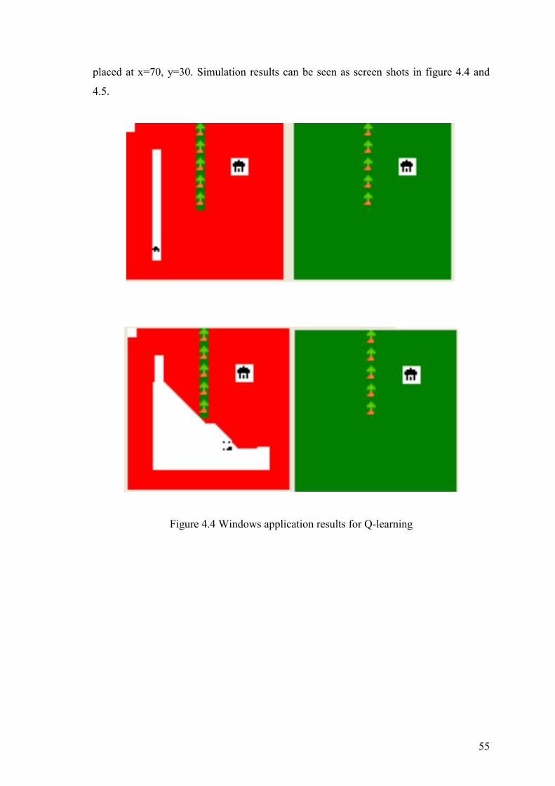
55
placed at x=70, y=30. Simulation results can be seen as screen shots in figure 4.4 and
4.5.
Figure 4.4 Windows application results for Q-learning
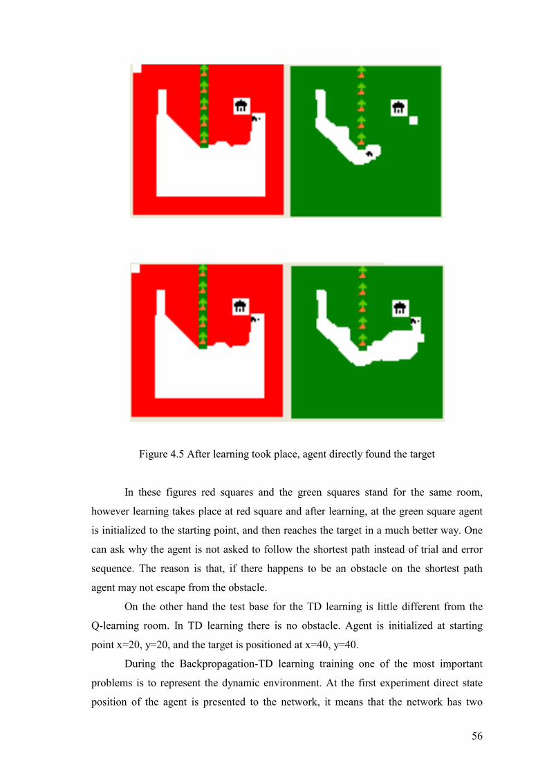
56
Figure 4.5 After learning took place, agent directly found the target
In these figures red squares and the green squares stand for the same room,
however learning takes place at red square and after learning, at the green square agent
is initialized to the starting point, and then reaches the target in a much better way. One
can ask why the agent is not asked to follow the shortest path instead of trial and error
sequence. The reason is that, if there happens to be an obstacle on the shortest path
agent may not escape from the obstacle.
On the other hand the test base for the TD learning is little different from the
Q-learning room. In TD learning there is no obstacle. Agent is initialized at starting
point x=20, y=20, and the target is positioned at x=40, y=40.
During the Backpropagation-TD learning training one of the most important
problems is to represent the dynamic environment. At the first experiment direct state
position of the agent is presented to the network, it means that the network has two
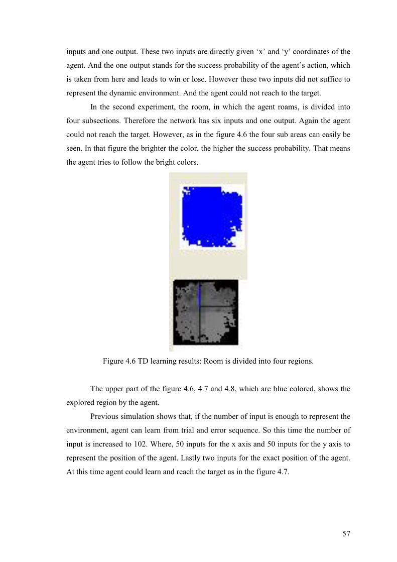
57
inputs and one output. These two inputs are directly given ‘x’ and ‘y’ coordinates of the
agent. And the one output stands for the success probability of the agent’s action, which
is taken from here and leads to win or lose. However these two inputs did not suffice to
represent the dynamic environment. And the agent could not reach to the target.
In the second experiment, the room, in which the agent roams, is divided into
four subsections. Therefore the network has six inputs and one output. Again the agent
could not reach the target. However, as in the figure 4.6 the four sub areas can easily be
seen. In that figure the brighter the color, the higher the success probability. That means
the agent tries to follow the bright colors.
Figure 4.6 TD learning results: Room is divided into four regions.
The upper part of the figure 4.6, 4.7 and 4.8, which are blue colored, shows the
explored region by the agent.
Previous simulation shows that, if the number of input is enough to represent the
environment, agent can learn from trial and error sequence. So this time the number of
input is increased to 102. Where, 50 inputs for the x axis and 50 inputs for the y axis to
represent the position of the agent. Lastly two inputs for the exact position of the agent.
At this time agent could learn and reach the target as in the figure 4.7.

58
Figure 4.7 After learning took place, agent is able to go directly.
If the learning parameters can be tuned appropriately, learning can take place
much faster.
Figure 4.8 If the learning parameters are changed appropriately, learning can take place
much faster.

59
CHAPTER 5
CONCLUSIONS Through this research, various AI methods are investigated. And their formal
definitions and fundamentals are given with their applications as well. Aim of this
research was to develop a system which interacts with its environment. And during this
interaction with the environment the system will be capable of gathering information
about its environment and response to the dynamic changes in a reasonable way.
In this thesis learning methods are divided into three main groups, these are
supervised algorithms, unsupervised algorithms and reinforcement learning in which the
genetic algorithms are included. MLP algorithms are utilized as supervised algorithms.
In the subsequent sections Backpropagation NNs, RBFNNs, and RBFLNs are
discussed. Their fundamentals are given and then their performance and robustness are
compared with each other. SONNs and K-means algorithms are discussed as
unsupervised methods. And, K-means algorithm is modified by author and it is shown
that this new modified K-means outperform the classic k-means algorithm.
Reinforcement learning is the most important subject of this thesis, since
reinforcement learning gives us an ability to teach the agent or system by its past
experience. Also the supervised and unsupervised methods are utilized to improve the
reinforcement learning. Finally, supervised methods are used as complementary
methods for reinforcement learning. In literature there are some other applications that
used unsupervised learning scheme with reinforcement learning.
Temporal difference method has studied intensively in the reinforcement
learning chapter, which was the method discussed in depth. Also the Q-learning method
is discussed and simulated. When the performance of these two reinforcement methods
are compared, for the simple one obstacle case Q-learning seams faster than TD
learning. However because of the memory usage of the Q-learning, generalization
capability is lower than the TD learning procedure. On the other hand training time of
the TD learning is too long because of the trial and error scheme. The navigation
application which is presented in this thesis takes between two and four hours according
to the initial position of the target and the agent. Also in literature TD-Backgammon
training time is given as several months.

60
In the future, training time must be decreased. In literature there is no way
formally presented to heal this training time problem for all cases. Also there is another
difficulty to implement the TD learning method to complex real world problems.
Connectionists TD structure needs many inputs to represent the environment and the
dynamic system. These problems are yet to be tackled as future work.

61
REFERENCES
[1] Widrow, B. and M. Hoff. “Adaptive Switching and Circuits,” Institute of Radio
Engineers WESCON convention record, part 4, (1960), 96-104.
[2] Kohonen, Teuvo. “Self-Organized Formation of Topologically Correct Feature
Maps,” Biological Cybernetics, 48, (1982), 59-69.
[3] M.A Aizerman, E.M. Braverman, and L.I. Rozonoer, “Theoretical foundations of
the potential function method in pattern recognition learning,” Automation and
Remote Control, 25, (1964), 821-837.
[4] O.A. Bashkirov, E.M. Braverman, and I.B. Muchnik, “Potential function algorithms
for pattern recognition learning machines,” Automation and Remote Control, 25,
(1964), 629-631.
[5] D.F. Sprecht, “A practical technique for estimating general regression surfaces,”
Report LMSC-6-79-68-6, Lockheed Missile and Space Co., Inc., Palo Alto, CA,
(1968).
[6] D.S. Broomhead, and D. Lowe, “Multivariable functional interpolation and adaptive
networks,” Complex Systems, 2, (1988), 321-335.
[7] J.E. Moody, and C.J. Darken, “Fast Learning in Networks of locally-tuned
processing units,” Neural Computation, 1(2), (1989), 281-294.
[8] Carl G. Looney, “Radial basis functional link nets and fuzzy reasoning”,
Neurocomputing, 48, (2002), 489–509
[9] Parzen, E. “On Estimation of a Probability Density Function and Mode,” Annals of
Mathematical Statistics, 33, (1962), 1065-1076.
[10] Specht, Donald. “Probabilistic Neural Networks,” Neural Networks, 3, (1990),
109-118.

62
[11] Ozdemir S., Karakurt M., "A Novel Hybrid Algorithm for Training ANNs".
International Symposium on Artificial Intelligence and Neural Networks, July
2003, Çanakkale.
[12] Rumelhart, D.E., Hinton, G.E., &Williams,R.J. ,Learning internal representations
by error propagation, In Parallel distributed processing ,(vol. 1), Cambridge,
MA:MIT Press, (1986).
[13] Bishop, C. Neural Networks for Pattern Recognition. New York: Oxford
University Press,(1995).
[14] Tani, G. J., & Fukumura, N. “Learning goal-directed sensory-based navigation of a
mobile robot,” Neural Networks, 7(3), (1994), 553-563.
[15] Rummery, G. A., Problem Solving with Reinforcement Learning, PhD thesis,
Cambridge University, (1995).
[16] Barto, A. G., Sutton, R.S., & Anderson, C. W. “Neuron like elements that can solve
difficult learning control problems,” IEEE Transactions on Systems, Man, and
Cybernetics, 13, (1983), 835-846.
[17] Sutton, R. S. (1984). Temporal credit assignment in reinforcement learning,
Doctoral dissertation, Department of Computer and Information Science,
University of Massachusetts, Amherst.
[18] Tesauro, G. J., “Practical issues in temporal difference learning,” Machine
learning, 8, (1992), 257-277.
[19] Tesauro, G. J. “Td-Gammon, a self teaching backgammon program, achieves
master-level play,” Neural Computation, 6(2), (1994), 215-219.
[20] Lin L. J. (1993). , Reinforcement Learning for Robots using neural networks, PhD
thesis, Carnegie Mellon University, Pittsburg, CMU-CS-93-103.

63
[21] Crites, R. H., & Barto, A. G. “Improving elevator performance using reinforcement
learning,” Neural Information Processing Systems, 8, (1996).
[22] Wedel, J., & Polani, D. ,Critic-based learning of actions with self organizing
feature maps, Technical Report NU-CCS-88-3, College of Computer Science of
Northeastern University, Boston, MA,(1996).
[23] Touzet, C. “Neural reinforcement learning for behavior synthesis,” Robotics and
Autonomous Systems, Special Issue on Learning Robots: The New Wave, 222,
(1997), 251-281.
[24] L. P. Kaelbling, M. L. Littman, A. W. Moore, “Reinforcement Learning: A
Survey”, Journal of Artificial Intelligence Research, 4, (1996), 237-285.
[25] Bertsekas, D. P. “Dynamic Programming and Optimal Control,” Athena Scientific,
Belmont, Massachusetts, 1, 2, (1995).
[26] Berry, D. A.,& Fristedt, B. , Bandit Problems: Sequential Allocation of
Experiments. Chapman and Hall, London, UK, (1985).
[27] Bellman, R. Dynamic Programming, Princeton University Press, Princeton, NJ,
(1957).
[28] Bertsekas, D. P., Dynamic Programming: Deterministic and Stochastic Models,
Prentice-Hall, Englewood Cliffs, NJ, (1987).
[29] Howard, R. A., Dynamic Programming and Markov Processes, The MIT Press,
Cambridge, MA, (1960).
[30] Puterman, M. L. ,Markov Decision Processes: Discrete Stochastic Dynamic
Programming, John Wiley & Sons, Inc., New York, NY, (1994).
[31] Sutton, R. S. “Learning to predict by the method of temporal differences,” Machine
Learning, 3 (1), (1988), 9-44.

64
[32] N. Baba , H. Suto., “Utilization of artificial neural networks and the TD-learning
method for constructing intelligent decision support systems,” European Journal
of Operational Research, 122, (2000), 501-508.
[33] Samuel. A. L. “Some studies in machine learning using the game of checkers,”
IBM Journal on Research and Development, 3, (1959), 210-229.
[34] Holland, J. H., Escaping brittleness: The possibilities of general purpose learning
algorithms applied to parallel rule-based systems, In R. S. Michalski, J. G.
Carbonell, & T. M. Mitchell (Eds.), Machine learning: An artificial intelligence
approach,2, Los Altos, CA: Morgan Kaufmann, (1986).
[35] Witten, I. H. “An adaptive optimal controller for discrete-time Markov
environments,” Information and Control, 34, (1977), 286-295.
[36] Booker, L. B., Intelligent behavior as an adaptation to the task environment,
Doctoral dissertation, Department of Computer and Communication Sciences,
University of Michigan, Ann Arbor, (1982).
[37] Hampson, S. E., A neural model of adaptive behavior, Doctoral dissertation,
Department of Information and Computer Science, University of California,
Irvine, (1983).
[38] Sutton, R. S., & Barto, A. G. “Toward a modern theory of adaptive networks:
Expectation and prediction,” Psychological Review, 88, (1981a), 135-171.
[39] Sutton, R. S., & Barto, A. G., A temporal-difference model of classical
conditioning, Proceedings of the Ninth Annual Conference of the Cognitive
Science Society, Seattle, WA: Lawrence Erlbaum, (1987) , p. 355-378.
[40] Gelperin, A., Hopfield, J. J., Tank, D. W., The logic of Limax learning, In A.
Selverston (Ed.), Model neural networks and behavior. New York: Plenum Press
(1985).

65
[41] Moore, J. W., Desmond, J. E., Berthier, N. E., Blazis, D. E. J., Sutton, R. S., &
Barto, A. G. “Simulation of the classically conditioned nictitating membrane
response by a neuron-like adaptive element: Response topography, neuronal firing
and interstimulus intervals,” Behavioral Brain Research, 21, (1986), 143-154.
[42] Klopf, A. H. (1987), A neuronal model of classical conditioning, (Technical Report
87-1139). OH: Wright-Patterson Air Force Base, Wright Aeronautical
Laboratories.
[43] Kemeny, J. G., & Snell, J. L., Finite Markov chains, New York: Springer-Verlag,
(1976).
[44] Watkins, C. J. C. H., Learning from Delayed Rewards, Ph.D., thesis, King's
College, Cambridge, UK, (1989).
[45] Watkins, C. J. C. H., & Dayan, P. “Q-learning,” Machine Learning, 8 (3), (1992),
279-292.
[46] Tsitsiklis, J. N. “Asynchronous stochastic approximation and Q-learning,” Machine
Learning, 16 (3), (1994).
[47] Jaakkola, T., Jordan, M. I., & Singh, S. P. “On the convergence of stochastic
iterative dynamic programming algorithms,” Neural Computation, 6 (6), (1994).
[48] Long-Ji Lin, “Self-Improving Reactive Agents Based On Reinforcement Learning,
Planning and Teaching,” Machine Learning, 8, (1992), 293-321
[49] Özel, T. Development of a predictive machining simulator for orthogonal metal
cutting process. 4 th International Conference on Engineering Design and
Automation, July 30- August 2, 2000, Orlando, Florida, USA., Department of
Industrial and Manufacturing Engineering Cleveland State University, Cleveland,
OH 44115, 2000.

66
[50] J. Rogers, in Object-oriented neural networks in C++, (Academic Press, Inc.
1997).

67
APPENDIX A
CODE INTERFACE SAMPLES These codes are developed from [50]. There are thousands of rows codes, hence
It is not possible to show all the codes.
class Base_Link // Base Neural-Network Link class
{
private:
static int ticket;
protected:
int id; // ID number for link
double *value; // Value(s) for Link
Base_Node *in_node; // Node instance link is comming from
Base_Node *out_node; // Node instance link is going to
int value_size;
public:
Base_Link( int size=1 ); // Constructor
~Base_Link( void ); // Destructor for Base Links
virtual void Save( ofstream &outfile );
virtual void Load( ifstream &infile );
inline virtual double Get_Value( int id=WEIGHT );
inline virtual void Set_Value( double new_val, int id=WEIGHT);
inline virtual void Set_In_Node( Base_Node *node, int id );
inline virtual void Set_Out_Node( Base_Node *node, int id );
inline virtual Base_Node *In_Node( void );
inline virtual Base_Node *Out_Node( void );
inline virtual char *Get_Name( void );
inline virtual void Update_Weight( double new_val );
inline int Get_ID( void );
inline virtual double In_Value( int mode=NODE_VALUE );

68
inline virtual double Out_Value( int mode=NODE_VALUE );
inline virtual double In_Error( int mode=NODE_ERROR );
inline virtual double Out_Error( int mode=NODE_ERROR );
inline virtual double Weighted_In_Value( int mode=NODE_VALUE );
inline virtual double Weighted_Out_Value( int mode=NODE_VALUE );
inline virtual double Weighted_In_Error( int mode=NODE_VALUE );
inline virtual double Weighted_Out_Error( int mode=NODE_VALUE );
inline virtual int Get_Set_Size( void );
inline virtual void Epoch( int mode=0 );
};
//------------------------------------------------------------------------------
class LList // Linked-List Support Class
{
private:
struct NODE
{
NODE *next, *prev;
Base_Link *element;
};
NODE *head,*tail,*curr;
int count;
public:
LList( void );
~LList( void );
int Add_To_Tail( Base_Link *element );
int Add_Node( Base_Link *element );
int Del_Node( void );
int Del( Base_Link *element );
int Find( Base_Link *element );
inline void Clear( void );
inline int Count( void );

69
inline void Reset_To_Head( void );
inline void Reset_To_Tail( void );
inline Base_Link *Curr( void );
inline void Next( void );
inline void Prev( void );
};
//--------------------------------------------------------------------------
class Base_Node // Base Neural-Network Node
{
private:
static int ticket;
protected:
int id; // Identification Number
double *value; // Value(s) stored by this node
int value_size; // Number of Values stored by this node
double *error; // Error value(s) stored by this node
int error_size; // Number of Error values stored by this node
LList in_links; // List for input links
LList out_links; // List for output links
public:
Base_Node( int v_size=1, int e_size=1 ); // Constructor
~Base_Node( void ); // Destructor
LList *In_Links( void );
LList *Out_Links( void );
virtual void Run( int mode=0 );
virtual void Learn( int mode=0 );
virtual void Epoch( int code=0 );
virtual void Load( ifstream &infile );
virtual void Save( ofstream &outfile);
inline virtual double Get_Value( int id=NODE_VALUE );
inline virtual void Set_Value( double new_val, int id=NODE_VALUE );

70
inline virtual double Get_Error( int id=NODE_ERROR );
inline virtual void Set_Error( double new_val, int id=NODE_ERROR );
inline int Get_ID( void );
inline virtual char *Get_Name( void );
void Create_Link_To( Base_Node &to_node, Base_Link *link );
virtual void Print( ofstream &out );
void Set_Centers (Base_Node *from_node);
double Compute_Distance();
double Compute_Sigma (Base_Node *Onode);
virtual double Transfer_Function();
double Compute_Min_Distance(Base_Node *Onode,int dump);
double Update_Sigma(double Lr,double output_error,double weight,
double node_value,double distance,double prev_sigma);
void Update_Center(double error,double lr);
virtual void Learn2(int mode, int dump, int additive, int inputs,double Lr);
friend void Connect( Base_Node &from_node, Base_Node &to_node,
Base_Link *link );
friend void Connect( Base_Node &from_node, Base_Node &to_node,
Base_Link &link );
friend void Connect( Base_Node *from_node, Base_Node *to_node,
Base_Link *link );
friend int Disconnect( Base_Node *from_node, Base_Node *to_node);
friend double Random( double lower_bound, double upper_bound );
};
//--------------------------------------------------------------------------
class Feed_Forward_Node : public Base_Node // This derived class provides
{ // a generic feed-forward
// neural-network node which
// can be used by the ADALINEs
// and Backprop networks.
protected:

71
virtual double Transfer_Function( double value );
public:
Feed_Forward_Node( int v_size=1, int e_size=1 ); // Constructor
virtual void Run( int mode=0 );
virtual char *Get_Name( void );
};
//--------------------------------------------------------------------------
class RB_Node : public Feed_Forward_Node
{
protected:
double *Center;
// virtual double Transfer_Function(double value/*Base_Node *Onode*/);
public:
RB_Node( int v_size=1, int e_size=0 ); // Default of 1 value set member
(NODE_VALUE)
virtual char *Get_Name( void );
void Set_Centers (Base_Node *from_node/*,Base_Node *to_node*/);
double Compute_Sigma (/*Base_Node *Main_Node,*/Base_Node *Onode);
double Update_Sigma(double Lr,double output_error,double weight,
double node_value,double distance,double prev_sigma);
virtual void Save(ofstream &outfile);
virtual void Load(ifstream &infile);
void Creat_Center(int num)
{
Center=new double[num];
for (int i=0;i<num;i++)
Center[i]=0.0;
}
void Set_Center(double new_val,int id) { Center[id]=new_val;}

72
double Get_Center(int id) {return Center[id];}
};
//-----------------------------------------------------------------------------
class RB_Link : public Base_Link
{
public:
RB_Link( int size=1 ); // default of 2 link value set members (WEIGHT,
DELTA)
virtual void Save( ofstream &outfile );
virtual void Load( ifstream &infile );
/* virtual char *Get_Name( void );
virtual void Update_Weight( double new_val );*/
};
//-----------------------------------------------------------------------------
class RB_Output_Node : public RB_Node
{
public:
RB_Output_Node( double lr, double mt, int v_size=3, int e_size=1 );
// default of 3 value set members (NODE_VALUE, LEARNING_RATE,
MOMENTUM)
// default of 1 error set member (NODE_ERROR)
virtual void Save(ofstream &outfile);
virtual void Load(ifstream &infile);
protected:
virtual double Compute_Error( int mode=0 );
virtual void Learn( int mode=0);
virtual void Learn2( int mode=0,int dump=0, int additive=0,int inputs=0,double
Lr=0);
virtual char *Get_Name( void );
virtual void Run (int mode=0);
};
//-----------------------------------------------------------------------------
class RB_Middle_Node : public RB_Node

73
{
public:
RB_Middle_Node(int v_size=10, int e_size=1 );
// default of 3 value set members
(NODE_VALUE,LEARNING_RATE,MOMENTUM)
// default of 1 error set member (NODE_ERROR)
// additionaly 5 centers
//and 1 sigma
//1 distance
virtual char *Get_Name( void );
void Set_Sigma(double new_val) {Sigma=new_val;}
double Get_Sigma() {return Sigma;}
double Compute_Distance(/*Base_Node *Node*/);
virtual double Transfer_Function(/*Base_Node *Onode*/);
// double Compute_Min_Distance(Base_Node *Onode,int dump);
virtual void Save(ofstream &outfile);
virtual void Load(ifstream &infile);
protected:
virtual double Compute_Error( int mode=0 );
double Sigma;
// virtual void Run(Base_Node *Node);
};
//-----------------------------------------------------------------------------
class RB_Additive_Node : public RB_Node
{
public:
RB_Additive_Node (double lr, double mt, int v_size=10, int e_size=1);
// default of 3 value set members
(NODE_VALUE,+LEARNING_RATE,+MOMENTUM)
// default of 1 error set member (NODE_ERROR)
// additionaly 5 centers
//and 1 sigma

74
//1 distance
virtual char *Get_Name( void );
void Set_Sigma(double new_val) {Sigma=new_val;}
double Get_Sigma() {return Sigma;}
double Compute_Distance(/*Base_Node *Node*/);
virtual double Transfer_Function(/*Base_Node *Onode*/);
// double Compute_Min_Distance(Base_Node *Onode,int dump);
virtual void Save(ofstream &outfile);
virtual void Load(ifstream &infile);
protected:
virtual double Compute_Error( int mode=0 );
double Sigma;
// virtual void Run(Base_Node *Node);
};
//--------------------------------------------------------------------------

75
APPENDIX B
TEST DATA
No:
Cutting
Speed Feed Time Fx Fz Flank Wear
1 200 0.05 10 150 110 38
2 200 0.05 20 180 120 48
3 300 0.05 60 200 120 114
4 200 0.1 10 220 190 38
5 200 0.1 20 230 150 58
6 200 0.1 60 270 190 59
7 250 0.1 10 200 150 51
8 300 0.1 20 230 190 89
9 300 0.05 40 180 120 81
10 200 0.05 80 180 140 79
11 250 0.05 50 220 200 89
12 200 0.05 60 250 120 74
13 300 0.05 20 130 80 58
14 200 0.05 100 220 90 84
15 250 0.05 20 150 120 53
16 250 0.05 60 220 120 99
17 300 0.1 10 210 140 56
18 200 0.1 40 260 190 71
19 200 0.1 30 250 210 66
20 200 0.05 70 210 110 76
21 250 0.05 40 220 130 79
22 200 0.05 30 150 10 53
23 250 0.1 20 230 170 81
24 200 0.05 40 200 120 66
25 200 0.05 50 210 120 66
Max 300 0.1 100 270 210 114
Min 200 0.05 10 130 10 38