Data-driven LPV modeling of continuous pulp digesters

TUE-CS-2013-002

D. Piga and R.Toth

May 1, 2013

Abstract

In this technical report, the LPV-IO identification techniques described in Kauven et al. [2013](Chapter 5) are applied in order to estimate an LPV model of a continuous pulp digester. The pulpdigester simulator (described in Moden [2011]) has been provided by ABB for benchmark studiesas part of its participation in the EU project Autoprofit.

1 Description of the continuous pulp digester

The continuous pulp digester is an upright standing tubular reactor (see Fig. 1) where wood chipstogether with withe liquor (a strongly aqueous solution of sodium hydroxine and sodium sulfide)are heated under pressure to dissolve the lignin in the wood chips and thus to obtain almost purecellulose fibers (wood pulp). These fibers are used to make all kinds of paper products.Wood chips and white liquor are fed continuously at the top, and the chips travel downwardsslowly, surrounded by free liquor and full of entrapped liquor in their porosities. Additional liquor,a mixture of white and wash liquor, is added at some points along the digester, and black liquor(spent mixture of white liquor and lignin) is extracted at a few points as well. The required heat forthe conversion is provided as latent heat by the feed liquor flows. The temperatures of the liquorflows can be controlled. In the bottom of the reactor, pulp and liquor leave the digester. Dependingon the zone of the reactor, the resulting flow of free liquor is counter-current or co-current withthe chip flow direction.The quality of the pulp is indicated by the amount of remaining lignin in the pulp. A measure forthis is the Kappa number. The smaller the Kappa number the higher is the quality of the pulp. Thequality is positively influenced by a longer resting (cooking) time of the pulp, higher temperaturesand larger liquor flows. It is worth remarking that in the process, though unwanted, some of thecellulose are dissolved, causing lower yield. Therefore, there is always a trade-off due to the factthat if the cook process is longer or the temperature is higher, more lignin is removed, but, at thesame time, more cellulose is lost.

1

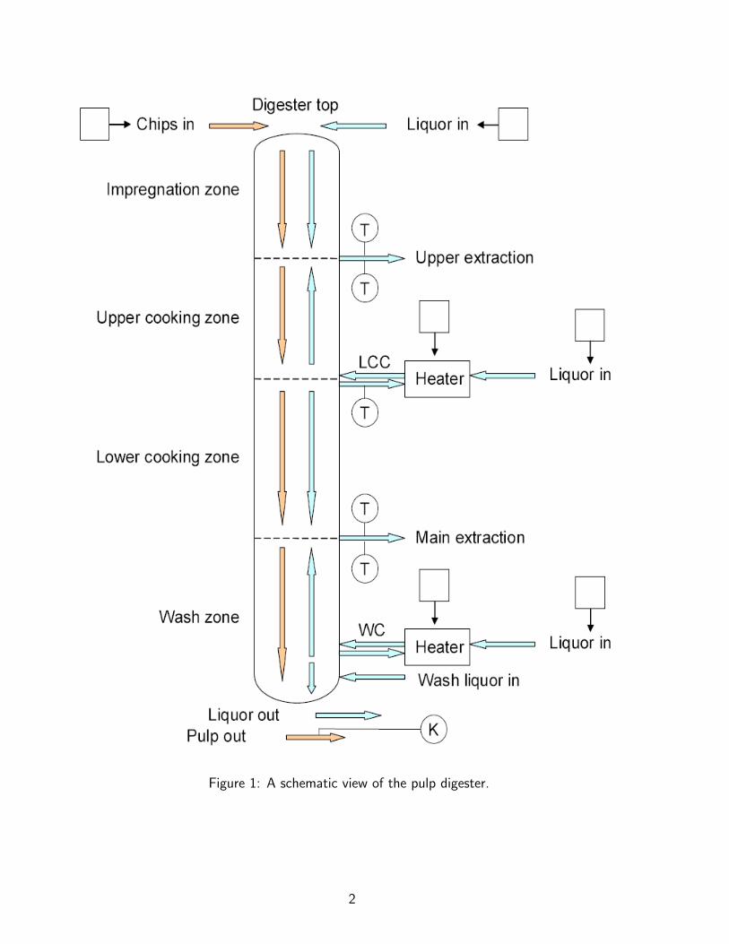
Figure 1: A schematic view of the pulp digester.

2

2 Simulator description

The basic core of the model implemented in the simulator provided by ABB is the extended Purduemodel introduced in Wisnewski et al. [1997], which consists of a set of nonlinear ordinary differentialequations (ODEs) modeling the three phases of the process: the solid phase of the wood chips, theentrapped-liquor phase, and the free-liquor phase. Exchange between the phases is also considered.

The manipulated variables (controller variables used to influence the process) are:

MV1 Temperature setpoint to LCC (lower cook circulation) heater;

MV2 Temperature setpoint to WC (wash circulation) heater;

MV3 Alkali-to-wood ratio with liquor feed to digester top;

MV4 Alkali-to-wood ratio with liquor feed to LCC;

MV5 Alkali-to-wood ratio with liquor feed to WC.

The disturbance variable (which is assumed to be measured) is:

D1 Chip feed rate.

The process variables (outputs of the process model) are:

PV1 Kappa number,

PV2 Liquor temperature in extraction from impregnation zone;

PV3 Liquor temperature in extraction from upper cooking zone;

PV4 Liquor temperature in extraction from lower cooking zone;

PV5 Liquor temperature in extraction from washing zone;

PV6 Liquor temperature in recirculation to LCC heater.

3 Simulation scenarios

The pulp digester is simulated for two different species of wood chips (hardwood and softwood)and for two different set-points for the Kappa number (Kappa number = 90 and Kappa number= 30). Then, the four different operating conditions considered in simulation are:

• Hardwood/Kappa number= 90;

• Softwood/Kappa number = 90;

• Hardwood/Kappa number = 30;

3

• Softwood/Kappa number = 30.

Details about the compositions of hardwood and softwood are available in Moden [2011].A closed-loop simulation is performed. More precisely, a linear MPC has been designed based on

the linearization of the Purdue model around the operating point. The considered (quadratic) costfunction penalizes the variations of all the manipulated variables and the deviations of the Kappanumber w.r.t. the setpoint. The temperature setpoints (i.e., MV1 and MV2) are constrained tobe smaller than 170 ◦C and the alkali-to-wood ratios (i.e., MV3, MV4 and MV5) are not allowedto be negative.

For each operating condition, the data are gathered by simulating the behavior of the pulpdigester for about 14 days (corresponding to 2000 samples measured with a time interval of 10

minutes). The chip feed rate is a (measurable) stochastic variable, normally distributed with amean of 0.025 m3/s and a standard deviation of 0.005 m3/s. The measurements of the Kappanumber are corrupted by an additive Gaussian white noise eo(t) with zero mean and standarddeviation 0.03. This corresponds to a signal-to-noise ratio (SNR) equal to about 8 db, where theSNR is defined as

SNR = 10 log10

2000∑t=1

(wo(t)− K

)22000∑t=1

e2o(t)

, (1)

where wo(t) is the noise-free measurement of the Kappa number at time t, while K is either 90

or 30, depending on the considered operating condition.The available data are splitted into two sets, i.e. an estimation data set DN (which consists of

the first N = 1500 data and is used to estimate a model of the pulp digester) and a validationdata set DV (which consists of the last NV = 500 data and is used to test the performance of theestimated model).

4 LPV model structure

The pulp digester dynamics are described by a MISO LPV model with:

• Kappa number (i.e., PV1) as output;

• MV1, MV2, MV3, MV4 and MV5 as inputs;

• Chip feed rate (i.e., DV1) and liquor temperature in extraction from impregnation zone (i.e.,PV2) as scheduling parameters.

The LPV model structure has been selected based on physical insights on the system behaviorand through a trial-and-error procedure, which aimed at maximizing the best fit rate (BFR) w.r.t.the validation data set DV , where the BFR is defined as

BFR = max{0, 1−‖y − y‖2‖y − y‖2

}, (2)

4

with y denoting the measured output (i.e., Kappa number), y the estimate of Kappa number, andy the sample mean of the (noise-corrupted) system output y in the validation data set. As physicalinsight for the choice of the regressors we used the residence time of the pulp in the different zonesof the pulp digester (cf. Moden [2011]). Hence, a certain number of recent inputs and outputs(different from the Kappa number) should not enter the regression vector. Using the BFR ascriterion, the trial-and-error procedure led to a model where the value of the Kappa number attime t depends on:

• Kappa number at time t − 1 and t − 2;

• MV1 at time t − 12, t − 13 and t − 14;

• MV2 at time t, t − 1 and t − 2;

• MV3 at time t − 12, t − 13 and t − 14;

• MV4 at time t − 32, t − 33 and t − 34;

• MV5 at time t, t − 1 and t − 2;

• DV1 at time t, t − 1 and t − 2;

• PV2 at time t − 20.

5 Obtained results

For each considered operating condition (i.e., Hardwood/Kappa number = 90; Softwood/Kappanumber = 90; Hardwood/Kappa number = 30; Softwood/Kappa number = 30), an LPV modelof the pulp digester is estimated through the identification algorithms described in Kauven et al.[2013]. It is important to point out that, when the parametric LPV identification approaches areapplied, an LPV model with affine dependencies on the scheduling variables is assumed.

In case of nonparametric LPV identification, Radial Basis Functions (RBFs) are used as kernelsK(�, �), i.e.,

K(p(j), p(k)) =exp

((p(j)− p(k))2

σ2

), (3a)

where p(k) is the value of the scheduling parameter vector at time k and σ > 0 is an hyper-parameter chosen by the user to control the width of the RBF. The value of σ is chosen througha cross-validation procedure, that is by maximizing (through an exhaustive search) the BFR (eq.(2)) w.r.t the validation data set DV. Of course, different values of σ are obtained in each of theconsidered operating conditions.

For the sake of comparison, an LTI model of the pulp digester is also estimated.First, the Hardwood/Kappa number = 90 operating condition is considered. The obtained

results are reported in Table 1, which shows the performance of the estimated models in terms ofBFR and MSE w.r.t. the validation data set DV, where the MSE is given by

MSE =1

N

NV∑t=1

(y(t)− y(t))2 . (4)

5

Table 1 also shows the computational time required by Matlab to estimate the model on a 2.40-GHz Intel Pentium IV with 3 GB of RAM. The outputs of the identified models over the validationset are plotted in Figs. 2(a)-7(a), together with the true values of Kappa number. Figs. 2(b)-7(b)show the differences between the estimates and the true values of Kappa number.

The other three operating conditions are then considered. The performance (in terms of BFR,MSE and required computational time) of the estimated models are summarized in Table 2, Table3 and Table 4. Only the outputs of the LPV models estimated through the open-loop parametricLPV identification approach are plotted (Figs. 8-10). It is important to remind that an LPV modelis identified at each operating condition.

The obtained results show that, besides having a low computational complexity, the parametricLPV identification algorithms achieved better performance in modeling the behavior of the pulpdigester in comparison to the LS-SVM based approaches. Furthermore, although the data aregathered in a closed-loop setting, the performance achieved by the open-loop identification schemesare comparable, and sometimes even better, than the ones achieved by the instrumental-variablebased algorithms. It is also important to point out that the estimated LPV models described moreaccurately the nonlinear dynamics of the pulp digester compared to LTI models. Therefore, theLPV modeling paradigm seems to be an interesting approach for improving the performance of theclosed-loop system.

References

D. Kauven, D. Piga, and R. Toth. Report on adaptive model refinement. Autoprofit Project,Deliverable 2.2, 2013.

P. E. Moden. Continuous pulp digester simulation model. ABB document: SECRC/AT/TR-2011/035, 2011.

P. A. Wisnewski, F. J. Doyle III, and F. Kayihan. Fundamental continuous-pulp-digester model forsimulation and control. AIChE journal, 43(12):3175–3192, 1997.

6

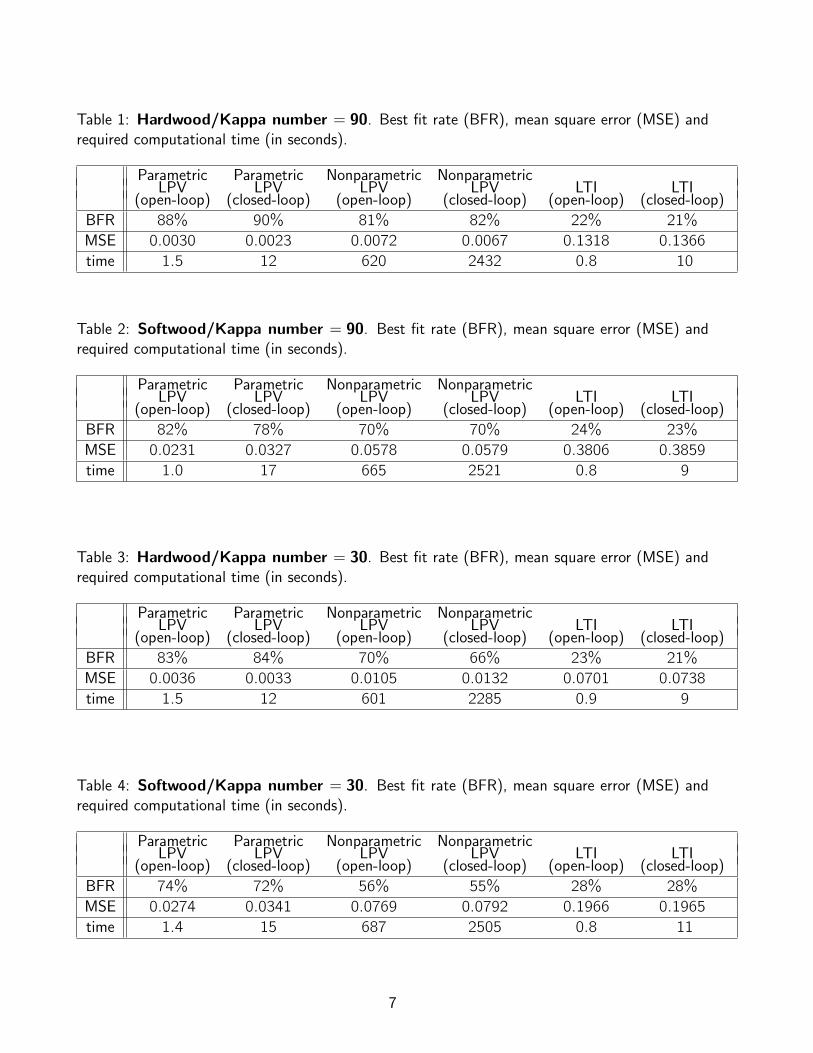
Table 1: Hardwood/Kappa number = 90. Best fit rate (BFR), mean square error (MSE) andrequired computational time (in seconds).

Parametric Parametric Nonparametric NonparametricLPV LPV LPV LPV LTI LTI

(open-loop) (closed-loop) (open-loop) (closed-loop) (open-loop) (closed-loop)

BFR 88% 90% 81% 82% 22% 21%

MSE 0.0030 0.0023 0.0072 0.0067 0.1318 0.1366

time 1.5 12 620 2432 0.8 10

Table 2: Softwood/Kappa number = 90. Best fit rate (BFR), mean square error (MSE) andrequired computational time (in seconds).

Parametric Parametric Nonparametric NonparametricLPV LPV LPV LPV LTI LTI

(open-loop) (closed-loop) (open-loop) (closed-loop) (open-loop) (closed-loop)

BFR 82% 78% 70% 70% 24% 23%

MSE 0.0231 0.0327 0.0578 0.0579 0.3806 0.3859

time 1.0 17 665 2521 0.8 9

Table 3: Hardwood/Kappa number = 30. Best fit rate (BFR), mean square error (MSE) andrequired computational time (in seconds).

Parametric Parametric Nonparametric NonparametricLPV LPV LPV LPV LTI LTI

(open-loop) (closed-loop) (open-loop) (closed-loop) (open-loop) (closed-loop)

BFR 83% 84% 70% 66% 23% 21%

MSE 0.0036 0.0033 0.0105 0.0132 0.0701 0.0738

time 1.5 12 601 2285 0.9 9

Table 4: Softwood/Kappa number = 30. Best fit rate (BFR), mean square error (MSE) andrequired computational time (in seconds).

Parametric Parametric Nonparametric NonparametricLPV LPV LPV LPV LTI LTI

(open-loop) (closed-loop) (open-loop) (closed-loop) (open-loop) (closed-loop)

BFR 74% 72% 56% 55% 28% 28%

MSE 0.0274 0.0341 0.0769 0.0792 0.1966 0.1965

time 1.4 15 687 2505 0.8 11

7

0 100 200 300 400 50088.5

89

89.5

90

90.5

91

91.5

Sample

Kap

pa

(a) Kappa number

0 100 200 300 400 500−0.4

−0.3

−0.2

−0.1

0

0.1

0.2

0.3

Sample

Err

or(b) Error

Figure 2: Hardwood/Kappa number = 90; Parametric LPV identification (open-loop): (a) trueKappa number (blue), estimated Kappa number (red); (b) difference between true Kappa numberand estimated Kappa number.

0 100 200 300 400 50088.5

89

89.5

90

90.5

91

91.5

Sample

Kap

pa

(a) Kappa number

0 100 200 300 400 500−0.4

−0.3

−0.2

−0.1

0

0.1

0.2

0.3

0.4

Sample

Err

or

(b) Error

Figure 3: Hardwood/Kappa number = 90; Parametric LPV identification (closed-loop): (a)true Kappa number (blue), estimated Kappa number (red); (b) difference between true Kappanumber and estimated Kappa number.

8

0 100 200 300 400 50088.5

89

89.5

90

90.5

91

91.5

Sample

Kap

pa

(a) Kappa number

0 100 200 300 400 500−0.4

−0.3

−0.2

−0.1

0

0.1

0.2

0.3

0.4

Sample

Err

or(b) Error

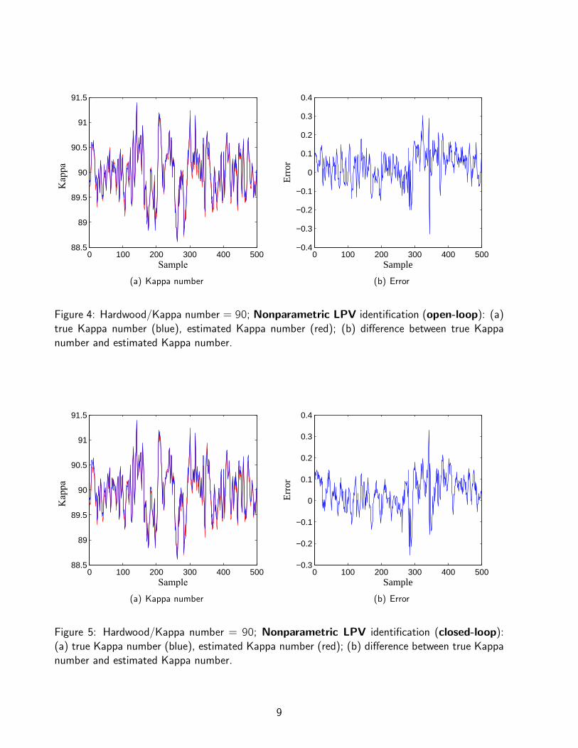
Figure 4: Hardwood/Kappa number = 90; Nonparametric LPV identification (open-loop): (a)true Kappa number (blue), estimated Kappa number (red); (b) difference between true Kappanumber and estimated Kappa number.

0 100 200 300 400 50088.5

89

89.5

90

90.5

91

91.5

Sample

Kap

pa

(a) Kappa number

0 100 200 300 400 500−0.3

−0.2

−0.1

0

0.1

0.2

0.3

0.4

Sample

Err

or

(b) Error

Figure 5: Hardwood/Kappa number = 90; Nonparametric LPV identification (closed-loop):(a) true Kappa number (blue), estimated Kappa number (red); (b) difference between true Kappanumber and estimated Kappa number.

9

0 100 200 300 400 50088.5

89

89.5

90

90.5

91

91.5

Sample

Kap

pa

(a) Kappa number

0 100 200 300 400 500−1.5

−1

−0.5

0

0.5

1

1.5

Sample

Err

or(b) Error

Figure 6: Hardwood/Kappa number = 90; LTI identification (open-loop): (a) true Kappa number(blue), estimated Kappa number (red); (b) difference between true Kappa number and estimatedKappa number.

0 100 200 300 400 50088.5

89

89.5

90

90.5

91

91.5

Sample

Kap

pa

(a) Kappa number

0 100 200 300 400 500−1.5

−1

−0.5

0

0.5

1

1.5

Sample

Err

or

(b) Error

Figure 7: Hardwood/Kappa number = 90; LTI identification (closed-loop): (a) true Kappanumber (blue), estimated Kappa number (red); (b) difference between true Kappa number andestimated Kappa number.

10

0 100 200 300 400 50087

88

89

90

91

92

93

Sample

Kap

pa

(a) Kappa number

0 100 200 300 400 500−1

−0.5

0

0.5

1

1.5

Sample

Err

or(b) Error

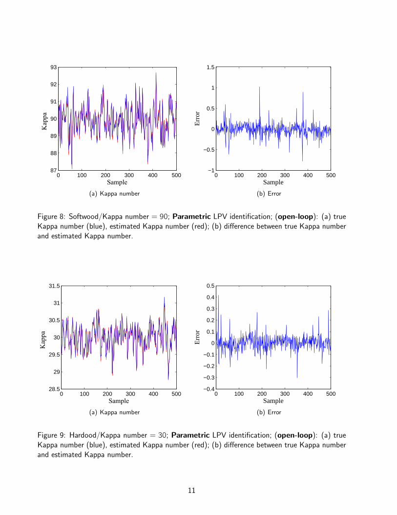
Figure 8: Softwood/Kappa number = 90; Parametric LPV identification; (open-loop): (a) trueKappa number (blue), estimated Kappa number (red); (b) difference between true Kappa numberand estimated Kappa number.

0 100 200 300 400 50028.5

29

29.5

30

30.5

31

31.5

Sample

Kappa

(a) Kappa number

0 100 200 300 400 500−0.4

−0.3

−0.2

−0.1

0

0.1

0.2

0.3

0.4

0.5

Sample

Err

or

(b) Error

Figure 9: Hardood/Kappa number = 30; Parametric LPV identification; (open-loop): (a) trueKappa number (blue), estimated Kappa number (red); (b) difference between true Kappa numberand estimated Kappa number.

11

0 100 200 300 400 50028

28.5

29

29.5

30

30.5

31

31.5

32

Sample

Kap

pa

(a) Kappa number

0 100 200 300 400 500−1

−0.5

0

0.5

1

1.5

Sample

Err

or

(b) Error

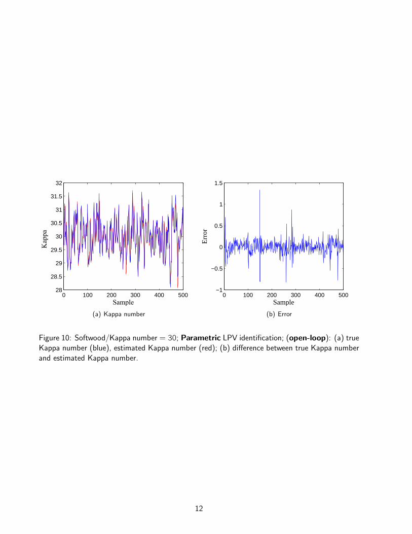
Figure 10: Softwood/Kappa number = 30; Parametric LPV identification; (open-loop): (a) trueKappa number (blue), estimated Kappa number (red); (b) difference between true Kappa numberand estimated Kappa number.

12