NREL is a national laboratory of the U.S. Department of Energy, Office of Energy Efficiency & Renewable Energy, operated by the Alliance for Sustainable Energy, LLC.

Contract No. DE-AC36-08GO28308

Data Collection for Current U.S. Wind Energy Projects: Component Costs, Financing, Operations, and Maintenance January 2011 – September 2011 M. Martin-Tretton, M. Reha, M. Drunsic, and M. Keim DNV Renewables (USA) Inc. Seattle, Washington

Subcontract Report NREL/SR-5000-52707 January 2012

NREL is a national laboratory of the U.S. Department of Energy, Office of Energy Efficiency & Renewable Energy, operated by the Alliance for Sustainable Energy, LLC.

National Renewable Energy Laboratory 1617 Cole Boulevard Golden, Colorado 80401 303-275-3000 • www.nrel.gov

Contract No. DE-AC36-08GO28308

Data Collection for Current U.S. Wind Energy Projects: Component Costs, Financing, Operations, and Maintenance January 2011 – September 2011 M. Martin-Tretton, M. Reha, M. Drunsic, and M. Keim DNV Renewables (USA) Inc. Seattle, Washington

NREL Technical Monitors: Paul Schwabe and Suzanne Tegen Prepared under Subcontract No. ADB-1-11427-00

Subcontract Report NREL/SR-5000-52707 January 2012

This publication received minimal editorial review at NREL.

NOTICE

This report was prepared as an account of work sponsored by an agency of the United States government. Neither the United States government nor any agency thereof, nor any of their employees, makes any warranty, express or implied, or assumes any legal liability or responsibility for the accuracy, completeness, or usefulness of any information, apparatus, product, or process disclosed, or represents that its use would not infringe privately owned rights. Reference herein to any specific commercial product, process, or service by trade name, trademark, manufacturer, or otherwise does not necessarily constitute or imply its endorsement, recommendation, or favoring by the United States government or any agency thereof. The views and opinions of authors expressed herein do not necessarily state or reflect those of the United States government or any agency thereof.

Available electronically at http://www.osti.gov/bridge

Available for a processing fee to U.S. Department of Energy and its contractors, in paper, from:

U.S. Department of Energy Office of Scientific and Technical Information P.O. Box 62 Oak Ridge, TN 37831-0062 phone: 865.576.8401 fax: 865.576.5728 email: mailto:reports@adonis.osti.gov

Available for sale to the public, in paper, from:

U.S. Department of Commerce National Technical Information Service 5285 Port Royal Road Springfield, VA 22161 phone: 800.553.6847 fax: 703.605.6900 email: orders@ntis.fedworld.gov online ordering: http://www.ntis.gov/help/ordermethods.aspx

Cover Photos: (left to right) PIX 16416, PIX 17423, PIX 16560, PIX 17613, PIX 17436, PIX 17721

Printed on paper containing at least 50% wastepaper, including 10% post consumer waste.

i

Data Collection for Current U.S. Wind Energy Projects: Component Costs, Financing and Operations and Maintenance

DNV Renewables (USA) Inc. 1809 7th Avenue, Suite 900 Seattle, WA 98101 USA Tel: 1-206-387-4200 Fax: 1-206-387-4201 http://www.dnv.com/windenergy

Prepared For: National Renewable Energy Laboratory 1617 Cole Boulevard Golden, Colorado 80401

Date of First Issue: May 24, 2011 Project No. PP004318

Report No.: DDRP0073 Organization Unit: ACGUS368

Version: Revision Date: October 10, 2011

Summary:

The National Renewable Energy Laboratory retained DNV to prepare this report to supplement the Excel workbook developed under subcontract no. AGB-1-11427 dated January 18, 2011.

Prepared by: Marina Martin-Tretton Technical Consultant

Signature

Prepared by: Meghan Reha Engineer

Signature

Prepared by: Michael W. Drunsic Head of Section

Signature

Verified & Approved by:

Michael Keim, Head of Section

Signature

ii

Acknowledgements

This work was funded by the U.S. Department of Energy’s (DOE’s) Wind and Water Power Program. The authors thank the individuals who reviewed various drafts of this report including Maureen Hand, Eric Lantz, Ben Maples, Paul Schwabe, and Suzanne Tegen of the National Renewable Energy Laboratory (NREL) and Jeroen Dolmans of DNV Renewables. The authors also offer their gratitude to Denise Fisher in NREL’s Communications Office for providing editorial support.

iii

Table of Contents

1 ABSTRACT ............................................................................................................................ 1

2 INTRODUCTION.................................................................................................................. 2

3 O&M COST MODEL SCENARIOS ................................................................................... 2

3.1 Scenarios - Method and Assumptions ........................................................................ 2

3.2 Results: Reference Component Replacement Scenario .............................................. 5

3.3 Results: High Failure, 100% Replacement, and Serial Failure Scenarios .................. 6

4 2010 COMPONENT COST UPDATE ................................................................................. 8

4.1 Component Costs – Methods and Assumptions ......................................................... 9

4.2 Results: Component Cost .......................................................................................... 12

4.3 O&M Arrangements ................................................................................................. 15

4.4 Component Cost 2005 – 2010 Historical Trend ....................................................... 15

5 PROJECT FINANCING ..................................................................................................... 17

5.1 Financing Structures ................................................................................................. 17

5.2 Capital Availability and Cost of Capital ................................................................... 21

5.3 Empirical Findings on Financial Metrics .................................................................. 22

6 REFERENCES ..................................................................................................................... 24

iv

Tables

Table 3-1. O&M Cost Model 20 Year Failure Rate Inputs for All Scenarios ............................ 4Table 3-2. Cost Comparisons to Reference Costs for Each Scenario ......................................... 6Table 4-1. Parts Categories by System ..................................................................................... 10Table 4-2. Annual Labor Rates ................................................................................................. 11Table 4-3. 2010 Component Cost Data 1.5 MW – 2.0 MW ..................................................... 13Table 4-4. 2010 Component Cost Data 2.1 MW – 3.0 MW ..................................................... 14Table 4-5. 2005 – 2010 Component Cost Trend ....................................................................... 16

Figures Figure 3-1. Reference Failure Rates, Five Year Average O&M Costs ...................................... 6Figure 4-1. Wind Turbine Manufacturers’ Share of 2010 U.S. Wind Power Installations ........ 9Figure 4-2. Cumulative Inflation Rate 2005 – 2010 ................................................................. 17

1

1 ABSTRACT

DNV Renewables (USA) Inc. (DNV) used an Operations and Maintenance (O&M) Cost Model to evaluate ten distinct cost scenarios encountered under variations in wind turbine component failure rates. The O&M Cost Model used in the analysis was developed for the National Renewable Energy Laboratory and is detailed in the 2008 report, Development of an Operations and Maintenance Cost Model to Identify Cost of Energy Savings for Low Wind Speed Turbines [1]. The analysis considers 1) a Reference Scenario using the default part failure rates within the O&M Cost Model, 2) High Failure Rate Scenarios that increase the failure rates of three major components (blades, gearboxes, and generators) individually, 3) 100% Replacement Scenarios that model full replacement of these components over a 20 year operating life, and 4) Serial Failure Scenarios that model full replacement of blades, gearboxes, and generators in years 4 to 6 of the wind project. DNV selected these scenarios to represent a broad range of possible operational experiences. The three High Failure Scenarios showed relatively little change from the Reference Scenario. The 100% Replacement and Serial Failure Scenarios showed much larger increases in overall costs relative to the High Failure and Reference Scenarios. The magnitude of the increase varied by component; the largest increase resulted when the blade failure rate was modified and the smallest increase resulted when the generator failure rate was modified. DNV updated the component cost data in the O&M Cost Model based on information from suppliers and actual receipts from recent component replacement work. A trend analysis comparing the 2010 component cost to data from 2005 shows no clear pattern of price changes and different changes by component type. Also in this report, DNV summarizes the predominant financing arrangements used to develop wind energy projects over the past several years and provides summary data on various financial metrics describing those arrangements. The summary is based on projects developed in 2010 and 2011. The financial metric information reflects a significant increase in financed projects using term debt and the monetized version of the investment tax credit since 2009, when compared to the number of projects financed using tax equity investments in 2006 and 2007. The review of these metrics suggests a more consistent debt market, with largely equivalent terms across projects, compared to tax equity financing arrangements that vary widely from project to project.

2

2 INTRODUCTION

The National Renewable Energy Laboratory (NREL) retained DNV under Subcontract No. AGB-1-11427 to prepare an Excel workbook with wind energy component replacement data for U.S. wind energy projects. The inputs included component replacement costs, financing metrics, and O&M parameters. This report provides a narrative description of DNV’s work under this agreement. It describes the model scenarios considered, the updated component costs from previous analyses, historical trends, and various aspects of project financing in 2010 and 2011.

3 O&M COST MODEL SCENARIOS

DNV created ten unique O&M scenarios to demonstrate the impact of various major component failure rates on O&M costs. The default rates and costs were based on data gathered from operating projects and industry component failure testing. The data is detailed in NREL's report, NREL/SR-500-40581, titled Development of an Operations and Maintenance Cost Model to Identify Cost of Energy Savings for Low Wind Speed Turbines, published in January 2008 (the O&M Model Report) [1]. This report accompanied the original model developed for NREL. It states, in part:

“The model estimates parts use by applying two types of failure rates to selected components, or categories of components. The first type of failure event is random, and is represented by a constant failure rate. The model assumes by default that 5% of the blades and gearboxes, and 10% of the generators, will fail over the 20-year life of the project because of uncontrollable circumstances such as lightning strikes, manufacturer defects, operational errors, or servicing omissions and errors.

The second type of failure event is wear out or deterioration, and is a two-parameter Weibull distribution. This distribution is commonly used in reliability studies as it allows for variation of the scale as well as the shape of the failure distribution. Weibull distributions are intended to describe failure rates for a given population of like components. Generally the most reliable data are obtained from exercising the components in actual or simulated conditions that are consistent over time. In an actual application, however, the parts that fail are replaced, so that the population eventually becomes a combination of components with varying periods of operation. At some point in time past the characteristic life, the instantaneous failure rate will oscillate about, and finally approach, a constant value.”

3.1 Scenarios - Method and Assumptions The O&M Cost Model requires input assumptions of project and turbine characteristics. In all scenarios, DNV assumed that the following inputs represent a typical project: 100 turbines, 36% net capacity factor, 1.5 MW turbine rating, 80 m hub height, electric pitch control, and partial power conversion. Specifying these project and turbine characteristics, DNV used the default failure rates within the model to construct a Reference Scenario to represent the baseline O&M costs. From a design

3

perspective, major components are certified to a 20 year design life. In practice, however, most turbine components experience failure before 20 years and the failure rate varies by component. Failure inputs to the O&M Cost Model can be modified by the user. The standard assumptions include a 5% catastrophic failure rate for blades and gearboxes and a 10% catastrophic failure rate for generators during the life of the turbine. Such catastrophic failures are considered to be the result of uncontrollable circumstances including, but not limited to, manufacturing defects and operational errors. In addition to the baseline failure rate, DNV modeled the considerable uncertainty of actual O&M costs due to factors not easily accounted for, such as variations in O&M practices, site conditions, like icing, extreme temperatures and environments, variations in individual turbine inflow conditions relative to the turbine's International Electrotechnical Commission (IEC) classification, and price ranges in the component costs. These uncertainties are estimated by evaluating O&M costs using a 30% higher parts failure rate and a 30% lower parts failure rate. DNV varied the blades, gearboxes, and generator failure rates from the default rates for three distinct scenarios. DNV selected these three components and scenarios based on proprietary wind industry data to represent a broad range of possible operational experiences. These permutations of components and scenarios resulted in nine additional cases. Once again, the uncertainty in O&M costs is represented with a 30% higher and lower component failure rate relative to the specific scenario discussed below. High Failure Rate Scenarios: DNV increased the individual component failure rate to three times (3x) the reference failure rate of a specified component. For example, the default failure rate for blades in the model is 5%; therefore, the High Blade Failure Scenario used a 15% failure rate for blades and the default failure rate for all other components. Similarly, the High Gearbox Failure Scenario used a 15% failure rate for gearboxes, and default failure rates for all other components. The High Generator Failure Scenario used a 30% failure rate for the generator, and default failure rates for all other components. 100% Replacement Scenarios: DNV increased the failure rate to 100% for a specified component, distributing the failures evenly throughout the entire 20 year project life. In the 100% Failure Scenarios, the 30% uncertainty band represents failures at 130% and 70% over 20 years. For example, in the 100% Blade Replacement Scenario, the baseline represents 300 blade replacements, or 15 replacements per year. While the 30% Higher Parts Failure Scenario represents 390 blade replacements, and the 30% Lower Parts Failure Scenario represents 210 blade replacements. The components experiencing 100% replacement have a zero defect rate after the replacement. Serial Defect Scenarios: DNV increased the component failure rate to 100%, distributing these failures throughout operating years 4 through 6. This scenario simulates how O&M costs are distributed in the event of a serial failure occurring outside of a warranty period. Components not experiencing serial failure use the default failure rates, which are applied over the entire project life. As with the 100% Replacement Scenarios, the components experiencing a serial defect have a zero defect rate after the serial defect remediation is complete. DNV assumed that the cost of serial replacements would be the cost of the components plus the cost of installation including a

4

crane, labor, and other associated costs. These costs were distributed over a typical replacement period of three years with 33 or 34 turbines receiving replacements per year. Years 4 to 6 were selected as representative operating years because they occur after a typical original equipment manufacturers (OEM) warranty period. The failure rate inputs to the O&M Cost Model for the scenarios described above are shown in Table 3-1.

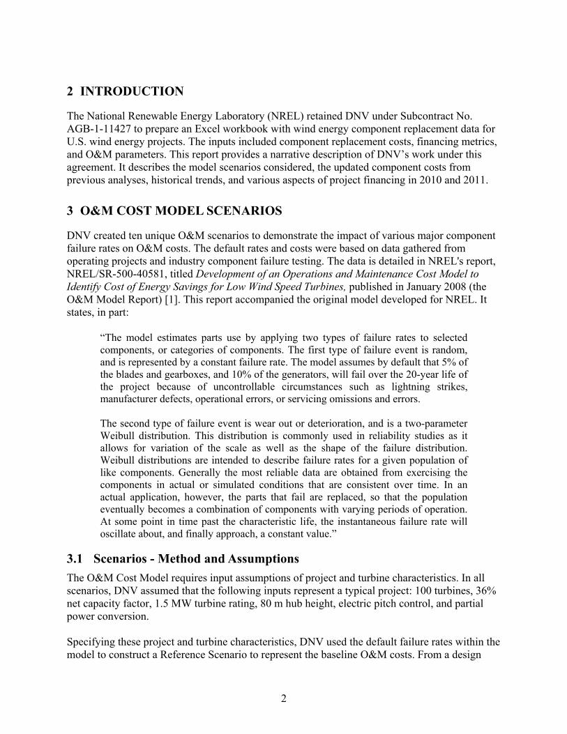
Table 3-1. O&M Cost Model 20 Year Failure Rate Inputs for All Scenarios

Blade Failure Rate (%)

Gearbox Failure Rate (%)

Generator Failure

Rate (%) Reference Scenario 5 5 10 High Blade Failure Scenario 15 5 10 High Gearbox Failure Scenario 5 15 10 High Generator Failure Scenario 5 5 30 100% Blade Failure Scenario 100 5 10 100% Gearbox Failure Scenario 5 100 10 100% Generator Failure Scenario 5 5 100 Serial Blade Failure Scenario* 100 5 10 Serial Gearbox Failure Scenario* 5 100 10 Serial Generator Failure Scenario* 5 5 100

* In the Serial Failure Scenarios, 100% component failures are modeled to occur in years 4 to 6 rather than evenly spread across the 20 year operating life (see description in text above).

Under all scenarios, DNV assumed that blades, gearboxes, and generators would be replaced as complete units. Rebuilt gearboxes and generators are common in the wind industry and the price of the replacement components in the O&M Cost Model is lower than the price of new components. Depending on the nature of the damage and when it is detected, gearbox maintenance ranges from repair or replacement of subcomponents to replacement of the entire gearbox. In many cases, subcomponents can be repaired prior to catastrophic failure, if the damage is identified in time. Such repairs often avoid the cost of crane deployment. Condition monitoring systems and inspections can help identify failures prior to a catastrophic event. It is uncommon to purchase refurbished blades; therefore, only new blade costs are considered in this analysis. The O&M Cost Model does not explicitly include economies of scale cost savings for crane costs. However, the cost of a crane rental is a significant contributor to the replacement cost of most major components. One way project operators reduce their costs is by performing multiple repairs that require a crane at the same time [1]. Therefore, DNV has included some economies of scale savings in this analysis. The general scheme used for crane economies of scale is that mobilization and demobilization costs are reduced per replacement job since the crane remains on site and in operation for an extended period of time, allowing these costs to be distributed over multiple jobs. In this analysis, DNV assumed that if more than four major failures occurred in a given year, all subsequent crane events for that year would be discounted. Larger discounts result as the number of crane events increases, until a minimum per-event crane cost is reached. As outlined in the O&M Model Report, turbines with integrated cranes that are capable of

5

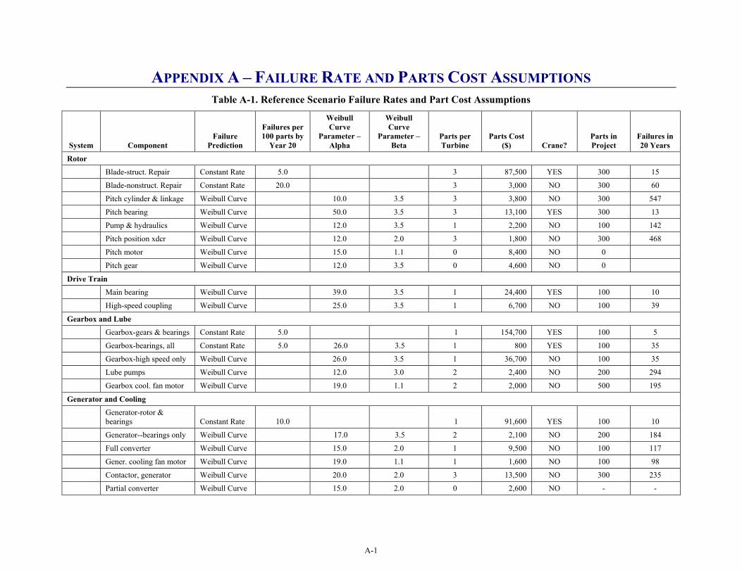
replacing wind turbine generators (e.g., nacelle mounted lifts) are not considered in the current model [1]. DNV used the updated component costs described in Section 4 of this report as input cost assumptions in the ten scenarios. In these scenarios, failures of blades, gearboxes, and generators were considered to be the most relevant major components. Additional components that could be considered include the bed-frame and main bearings. However, replacement of these components is rare compared to the replacement of blades, gearboxes, and generators. In addition to other components, two invariable cost items in the above scenarios are regularly scheduled maintenance (included through the labor budget and the consumables line items in the model) and a small budget for the maintenance of roads, meteorological equipment, and other facility maintenance. These items are held constant across the scenarios. Substation maintenance costs are not currently included in the model. These costs are highly variable from project to project and, in some cases, are borne by the off-taking utility instead of the project. There are various other costs when operating a wind project, such as insurance, taxes, and purchased electricity, that are not included in the model. A full listing of all component failure rates and cost assumptions is in Appendix A.

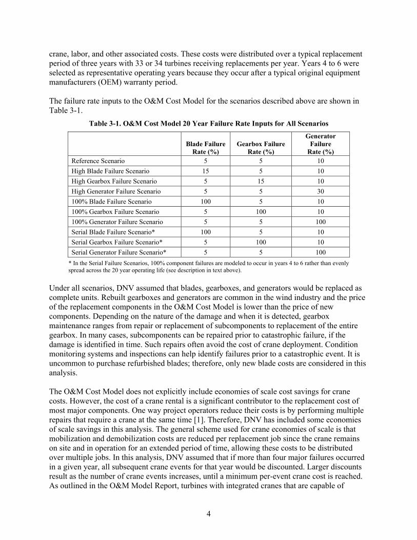
3.2 Results: Reference Component Replacement Scenario The results of the Reference Scenario are presented in Figure 3-1 as five year average O&M costs. As previously described, the uncertainty in the O&M costs is represented by the 30% higher and 30% lower parts failure rate band. The Reference Scenario results show increasing O&M costs over time. There is a slightly greater difference between the baseline and the 30% high case than between the baseline and the 30% low case due to the accelerated parts failures in the 30% high case which leads to a non-linear compounding effect in the total number of components replaced over 20 years.

6

Figure 3-1. Reference Failure Rates, Five Year Average O&M Costs

3.3 Results: High Failure, 100% Replacement, and Serial Failure Scenarios The results of the High Failure, 100% Replacement and Serial Failure Scenarios are shown in Table 3-2 and in Figure 3-2. In Figure 3-2, the High Failure, 100% Replacement and Serial Failure Scenarios are shown as solid black lines, while the 30% cost uncertainty band is shown with dashed black lines. For comparison purposes, the Reference Scenario is presented as solid grey lines while the uncertainties are shown as dashed grey lines. The Reference Scenario is identical in each plot.

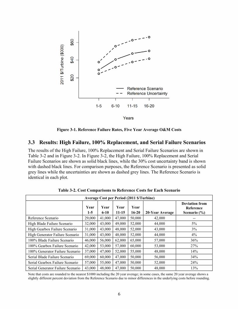
Table 3-2. Cost Comparisons to Reference Costs for Each Scenario

Average Cost per Period (2011 $/Turbine)

Year 1-5

Year 6-10

Year 11-15

Year 16-20 20-Year Average

Deviation from Reference

Scenario (%)

Reference Scenario 29,000 41,000 47,000 50,000 42,000 -- High Blade Failure Scenario 32,000 43,000 49,000 52,000 44,000 5% High Gearbox Failure Scenario 31,000 43,000 48,000 52,000 43,000 3% High Generator Failure Scenario 31,000 43,000 48,000 52,000 44,000 4% 100% Blade Failure Scenario 46,000 56,000 62,000 65,000 57,000 36% 100% Gearbox Failure Scenario 42,000 53,000 57,000 60,000 53,000 27% 100% Generator Failure Scenario 37,000 47,000 52,000 55,000 48,000 14% Serial Blade Failure Scenario 69,000 60,000 47,000 50,000 56,000 34% Serial Gearbox Failure Scenario 57,000 55,000 47,000 50,000 52,000 24% Serial Generator Failure Scenario 43,000 48,000 47,000 50,000 48,000 13% Note that costs are rounded to the nearest $1000 including the 20 year average; in some cases, the same 20 year average shows a slightly different percent deviation from the Reference Scenario due to minor differences in the underlying costs before rounding.

7

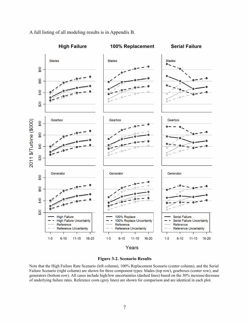
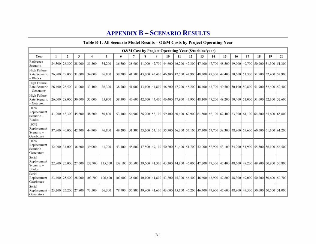
A full listing of all modeling results is in Appendix B.

Figure 3-2. Scenario Results

Note that the High Failure Rate Scenario (left column), 100% Replacement Scenario (center column), and the Serial Failure Scenario (right column) are shown for three component types: blades (top row), gearboxes (center row), and generators (bottom row). All cases include high/low uncertainties (dashed lines) based on the 30% increase/decrease of underlying failure rates. Reference costs (grey lines) are shown for comparison and are identical in each plot.

8

Comparing across scenarios (i.e., columns in Figure 3-2), there is only a minor difference between the High Failure Scenarios and the Reference Scenario, while the 100% Replacement Scenarios and the Serial Failure Scenarios illustrate significant differences from the Reference Scenario. When compared to the 100% Failure Rate Scenario, the Serial Defect Scenario for each component shows slightly lower 20 year average costs. This is primarily driven by the significantly discounted crane costs in the Serial Defect Scenarios as compared to the 100% Failure Rate Scenarios. The evolution of these costs over time is quite different between the 100% Replacement Scenarios, in which replacements are spread evenly across 20 years, and the Serial Failure Scenarios, in which replacements are concentrated in years 4 to 6. In the 100% Replacement Scenarios, costs increases from major component failures are incurred over all 20 years. In the Serial Failures Scenarios, the average O&M costs increases primarily in years 1 to 5 and years 6 to 10. The shape of the cost distribution changes slightly depending on the component selected. For example, in the Serial Failure Scenario, the cost of blades sharply decreases in per turbine O&M cost from the first five years to the last five years. The 200 blades replaced in years 4 and 5 increases the average in years 1 to 5. The 100 blades replaced in year 6 increases the average for years 6 to 10, but replacements are lower than in the first five years. No blades were replaced in years 11 to 20, resulting in significantly lower costs relative to the first 10 years. By comparison, the Gearbox and Generator Serial Failure Scenarios show much shallower declines in O&M costs over the first 15 years. Replacing a set of blades is more expensive than replacing a single gearbox or generator and the default generator failure rate (10%) is higher than the default blade failure rate (5%). There are only minor differences between the Reference Scenario and the High Failure Scenarios for each of the three components (on average less than 5% over 20 years). For the 100% Replacement Scenarios and Serial Failure Scenarios, the largest cost differences relative to the Reference Scenario are for blades, followed by gearboxes, followed by a relatively smaller difference for generators. Several factors contribute to the blade’s higher O&M costs relative to the gearbox and generator. The modeled project has 300 blades, as compared to 100 gearboxes and 100 generators. A set of three blades costs more than a single gearbox or generator. This accounts for a significant portion of the higher O&M cost. Also, this scenario assumes the blades must be purchased new, and therefore, does not consider any savings associated with using refurbished components or possible discounts for buying multiple blade sets.

4 2010 COMPONENT COST UPDATE

DNV compiled annual component cost data in the form of price lists, from the years 2005 through 2010, from the leading turbine manufacturers in the U.S. market. DNV updated the component cost data to capture some of the changes in wind project costs since the original O&M Model Report was published in early 2008 [1]. These data, from O&M replacement part price lists, are used with the permission of the turbine operators. Due to confidentiality agreements with price list contributors, individual owners of the manufacturers' price lists are not disclosed. However, the component cost data analyzed in this report are representative of close to

9

90% of U.S. wind turbines installed in 2010 [2]. Wind turbine manufacturers' U.S. market share in 2010 is shown in Figure 4-1.

GE Wind43%

Vestas17%

Siemens13%

Mitsubishi10%

Gamesa6%

Suzlon Group

6%

Nordex3% Others

2%

2010 United States Market Share% of 6,334 MW Total Installed

Figure 4-1. Wind Turbine Manufacturers’ Share of 2010 U.S. Wind Power Installations

Source: U.S. Wind Industry Annual Market Report Year Ending 2010 [2] Using these replacement costs as data inputs, turbine characteristics, and the year when the pricelists were issued, DNV calculated average turbine component costs, component cost ranges, estimated labor costs, and crane costs. The data are sorted into two main categories based on turbine rating:

• Wind turbine rating of 1.5 - 2.0 MW

• Wind turbine rating of 2.1 - 3.0 MW The resulting component, labor, and crane costs were used to update the inputs to the O&M Cost Model. The same list of components that were part of the original O&M Cost Model were populated with updated inputs to generate 2010 cost values for the scenarios discussed earlier in this report. It is important to note that, due to the nature of the model and the use of replacement parts price lists, the component cost values should not be interpreted as a bottom up calculation of the initial capital cost of a wind turbine.

4.1 Component Costs – Methods and Assumptions As shown in Table 4-1, the various replacement parts are categorized as the rotor, drive train, gearbox and lubrication, generator and cooling, brakes and hydraulics, yaw system, control system, electrical and grid, or miscellaneous. These categories are exclusive of consumables. Replacement parts (including mechanical, electrical, and hydraulic components) are those that wear or deteriorate during normal use. For example, gearboxes are a mechanical wear item, but

10

the main shaft and bedplate are not.

Table 4-1. Parts Categories by System

Rotor Blades, pitch bearings, pitch actuators

Drive train Main bearing, seals, couplings

Gearbox and lubrication Gearbox, lube pump, cooling system

Generator and cooling Generator, power converter, cooling system

Brakes and hydraulics Hydraulics, calipers, shoes

Yaw system Calipers, wear pads

Control system CPU, interface modules, sensors

Electrical and grid Contactors, circuit breakers, relays, capacitors

Miscellaneous Hardware, other small mechanical, hydraulic and electrical parts not identified specifically

The components included in the generic configuration represent the current state of the art for modern turbines currently being supplied. The assumptions for each component category are described below. Rotor: The rotor is three-bladed and each blade has independent pitch. The pitch bearings are the rolling-element type, and are periodically lubricated with grease. The pitch mechanism may be one of two types: 1) a hydraulic pitch system, which includes a pitch cylinder, proportional valve, crank arm mechanism, accumulator, and displacement transducer for each blade; or (2) an electric pitch system, which includes a motor with a position encoder, gear reducer, electronic drive, and backup battery bank for each blade. The pump and position controller are common for all three mechanisms (i.e., one per blade). Drive train: The drive train consists of a main shaft supported by two main bearings, coupled to the gearbox using a hydraulic shrink coupling. A composite tube, with flexure connections, is used to couple the gearbox to the generator. Gearbox and lubrication: The gearbox is a combination planetary/helical unit, with an integral lubrication system and fluid cooler system. The gearbox is suspended from the bedplate with elastomeric bushings. Generator and cooling: The generator is a single-speed, induction type. The variable-speed machine includes a wound rotor and slip-rings. Cooling is provided by an integral forced-air system. Brakes and hydraulics: The brake is a caliper-type system located on the high-speed shaft of the gearbox. A dedicated hydraulic system provides pressure for the calipers. The brake is used only for parking, since the primary rotor brake is the blade pitch system.

11

Yaw system: The yaw bearing is a sliding-bearing type, with spring-applied calipers for stabilization. The surfaces are periodically lubricated with grease. The yaw drives are electric-motor driven in a multiple-reduction gearbox. The number and size of the yaw drives increases with turbine size. Control system: The control and monitoring system consists of a main controller in the turbine base, a remote controller in the nacelle, and another in the hub. The base unit contains a user interface and display. Control sensors include wind measurement instruments, rotor speed control, and power/grid monitoring transducers. Sensors specific to monitoring component condition are included in that category. Electrical and grid: The turbine switchgear consists of a main breaker/disconnect, a line contactor for the generator power, and smaller contactors and circuit breakers for ancillary systems and power factor correction capacitors. A soft-starter is included for connecting to the grid for constant-speed machines. Miscellaneous: This category includes a value for miscellaneous parts not specifically identified elsewhere, such as hardware, small hydraulics, and small electrics. Parts costs for each of the generic turbine sizes were estimated from machine cost data. In some cases, these data were drawn from manufacturers’ price lists; in other cases, they were derived from actual receipts. The former data set is subject to an indeterminate mark-up; the latter may reflect a limited scope of supply. In addition to the component categories above, the O&M Cost Model includes a labor cost category. It includes the staff dedicated to turbine maintenance including regularly scheduled, unscheduled, and major maintenance. The calculation assumes the hourly rates for site staff show in Table 4-2. These are representative of rates at operating projects. Technician rates usually vary by skill level and experience, and often a crew consists of a senior-level technician paired with a junior-level technician. The rates represent average values for a crew. Local rates can vary by 25% and depend on the local labor market. The impact of labor rates on overall O&M costs is a function of the time required for repairs.

Table 4-2. Annual Labor Rates

Category Base Burdened @ 35% Junior Technician $31 $48 Senior Technician $49 $75

Source: DNV Update to Original O&M Cost Model [1]

Typically, the lead time to procure the crane and the components is longer than the time it takes to install a new major component. Total return-to-service time can be significantly longer than the time required for labor for the repair. As examples, a blade, gearbox, or generator can be replaced by experienced technicians in approximately 3-5 days, weather permitting, once the

12

crane has arrived on site. Smaller components typically can be replaced in a few hours. Downtime for these components can be minimized by maintaining a good spare parts inventory. Finally, the model assumes that the wind energy facility rents a crane for any major replacement, and that the replacements will occur on a per-unit basis. Crane rental costs are driven by crane capacity and mobilization time. Two common crane types—conventional crawler cranes and truck-mounted cranes—are appropriate for wind turbine component replacements. The cost for a crawler crane is driven by mobilization, as the crane and boom are shipped in pieces and require 10 to 20 truckloads, depending on height. Hydraulic truck-mounted cranes use a telescopic boom and require only one to three additional loads for counterweights. They are significantly cheaper to mobilize, but generally cost more per hour. Conventional cranes are sometimes available in a truck-mounted version, but still require multiple loads for the lattice boom and jibs.

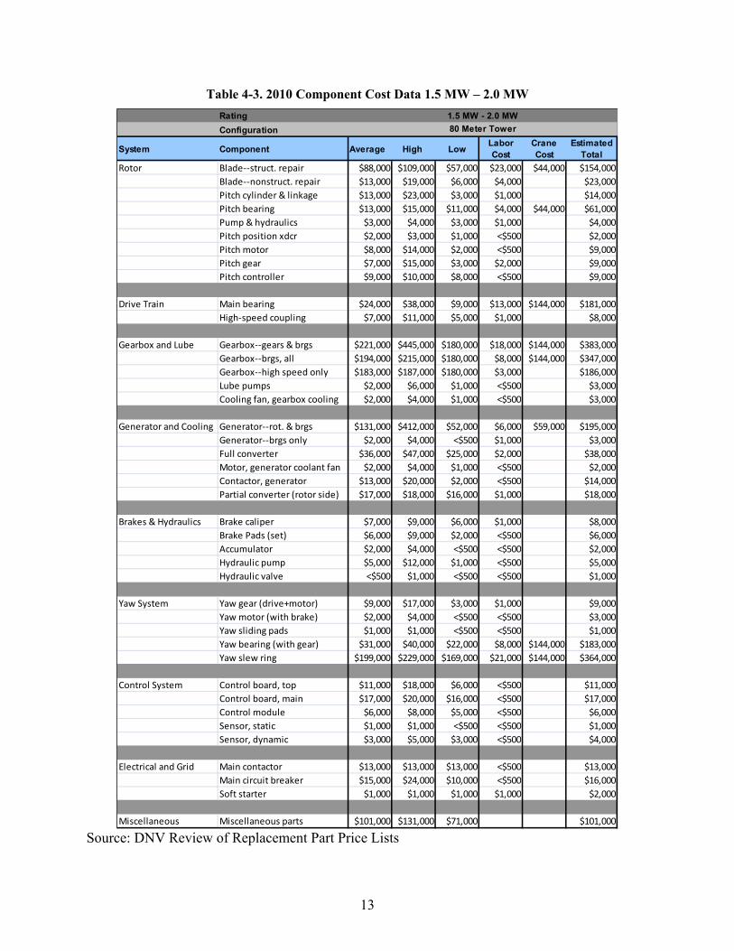
4.2 Results: Component Cost The results of the 2010 component cost data analysis are presented in Table 4-3 and 4-4. Average, maximum, and minimum costs are provided for each component, as well as the per event labor costs associated with the repair or replacement of the component, and the per event costs associated with crane mobilization and deployment (for components where crane use is required). Finally, the estimated total per event component replacement cost is provided; this is the combined average cost of the component, labor and, if applicable, crane costs. Amounts shown are rounded to represent reasonable levels of precision. In some cases, the rounded per-event totals do not equal the sum of the rounded parts, labor, and crane costs because the totals were rounded after summing the inputs. Major component cost data on the two categories discussed in this report, 1.5-2.0 MW and 2.1-3.0 MW machines, are biased toward the predominant turbines in the U.S. market today. Typically, the cost of major components and mechanical equipment associated with them will scale up relative to size. In particular, crane costs are sensitive to hub height and component weight. However, the rotor diameter, the complexity of control systems, and the overall quality of components varies based on different manufacturers; thus, a linear cost relation cannot be established for all components. Where no price list data inputs were available, such as the cost of the gearbox high speed section for turbines in the 2.0 MW to 3.0 MW range, the space was left blank to avoid providing misleading information.

13

Table 4-3. 2010 Component Cost Data 1.5 MW – 2.0 MW RatingConfiguration

System Component Average High Low Labor Cost

CraneCost

EstimatedTotal

Rotor Blade--struct. repair $88,000 $109,000 $57,000 $23,000 $44,000 $154,000Blade--nonstruct. repair $13,000 $19,000 $6,000 $4,000 $23,000Pitch cylinder & linkage $13,000 $23,000 $3,000 $1,000 $14,000Pitch bearing $13,000 $15,000 $11,000 $4,000 $44,000 $61,000Pump & hydraulics $3,000 $4,000 $3,000 $1,000 $4,000Pitch position xdcr $2,000 $3,000 $1,000 <$500 $2,000Pitch motor $8,000 $14,000 $2,000 <$500 $9,000Pitch gear $7,000 $15,000 $3,000 $2,000 $9,000Pitch controller $9,000 $10,000 $8,000 <$500 $9,000

Drive Train Main bearing $24,000 $38,000 $9,000 $13,000 $144,000 $181,000High-speed coupling $7,000 $11,000 $5,000 $1,000 $8,000

Gearbox and Lube Gearbox--gears & brgs $221,000 $445,000 $180,000 $18,000 $144,000 $383,000Gearbox--brgs, all $194,000 $215,000 $180,000 $8,000 $144,000 $347,000Gearbox--high speed only $183,000 $187,000 $180,000 $3,000 $186,000Lube pumps $2,000 $6,000 $1,000 <$500 $3,000Cooling fan, gearbox cooling $2,000 $4,000 $1,000 <$500 $3,000

Generator and Cooling Generator--rot. & brgs $131,000 $412,000 $52,000 $6,000 $59,000 $195,000Generator--brgs only $2,000 $4,000 <$500 $1,000 $3,000Full converter $36,000 $47,000 $25,000 $2,000 $38,000Motor, generator coolant fan $2,000 $4,000 $1,000 <$500 $2,000Contactor, generator $13,000 $20,000 $2,000 <$500 $14,000Partial converter (rotor side) $17,000 $18,000 $16,000 $1,000 $18,000

Brakes & Hydraulics Brake caliper $7,000 $9,000 $6,000 $1,000 $8,000Brake Pads (set) $6,000 $9,000 $2,000 <$500 $6,000Accumulator $2,000 $4,000 <$500 <$500 $2,000Hydraulic pump $5,000 $12,000 $1,000 <$500 $5,000Hydraulic valve <$500 $1,000 <$500 <$500 $1,000

Yaw System Yaw gear (drive+motor) $9,000 $17,000 $3,000 $1,000 $9,000Yaw motor (with brake) $2,000 $4,000 <$500 <$500 $3,000Yaw sliding pads $1,000 $1,000 <$500 <$500 $1,000Yaw bearing (with gear) $31,000 $40,000 $22,000 $8,000 $144,000 $183,000Yaw slew ring $199,000 $229,000 $169,000 $21,000 $144,000 $364,000

Control System Control board, top $11,000 $18,000 $6,000 <$500 $11,000Control board, main $17,000 $20,000 $16,000 <$500 $17,000Control module $6,000 $8,000 $5,000 <$500 $6,000Sensor, static $1,000 $1,000 <$500 <$500 $1,000Sensor, dynamic $3,000 $5,000 $3,000 <$500 $4,000

Electrical and Grid Main contactor $13,000 $13,000 $13,000 <$500 $13,000Main circuit breaker $15,000 $24,000 $10,000 <$500 $16,000Soft starter $1,000 $1,000 $1,000 $1,000 $2,000

Miscellaneous Miscellaneous parts $101,000 $131,000 $71,000 $101,000

1.5 MW - 2.0 MW80 Meter Tower

Source: DNV Review of Replacement Part Price Lists

14

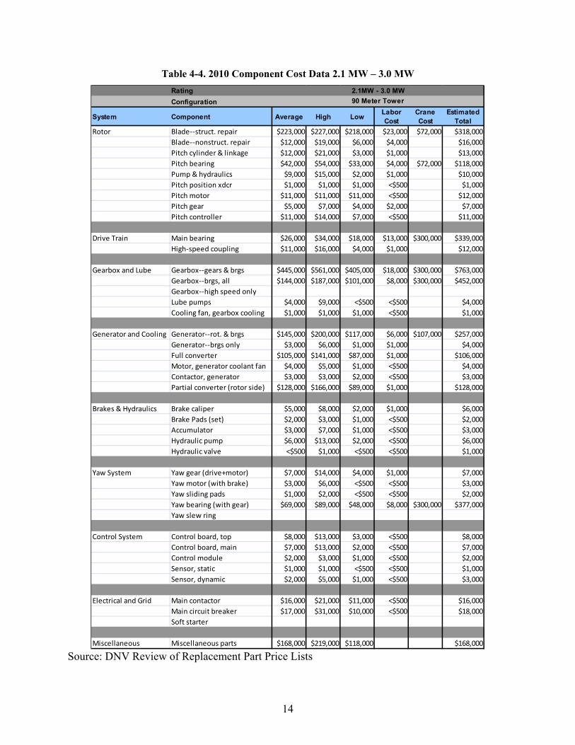
Table 4-4. 2010 Component Cost Data 2.1 MW – 3.0 MW RatingConfiguration

System Component Average High Low Labor Cost

CraneCost

EstimatedTotal

Rotor Blade--struct. repair $223,000 $227,000 $218,000 $23,000 $72,000 $318,000Blade--nonstruct. repair $12,000 $19,000 $6,000 $4,000 $16,000Pitch cylinder & linkage $12,000 $21,000 $3,000 $1,000 $13,000Pitch bearing $42,000 $54,000 $33,000 $4,000 $72,000 $118,000Pump & hydraulics $9,000 $15,000 $2,000 $1,000 $10,000Pitch position xdcr $1,000 $1,000 $1,000 <$500 $1,000Pitch motor $11,000 $11,000 $11,000 <$500 $12,000Pitch gear $5,000 $7,000 $4,000 $2,000 $7,000Pitch controller $11,000 $14,000 $7,000 <$500 $11,000

Drive Train Main bearing $26,000 $34,000 $18,000 $13,000 $300,000 $339,000High-speed coupling $11,000 $16,000 $4,000 $1,000 $12,000

Gearbox and Lube Gearbox--gears & brgs $445,000 $561,000 $405,000 $18,000 $300,000 $763,000Gearbox--brgs, all $144,000 $187,000 $101,000 $8,000 $300,000 $452,000Gearbox--high speed onlyLube pumps $4,000 $9,000 <$500 <$500 $4,000Cooling fan, gearbox cooling $1,000 $1,000 $1,000 <$500 $1,000

Generator and Cooling Generator--rot. & brgs $145,000 $200,000 $117,000 $6,000 $107,000 $257,000Generator--brgs only $3,000 $6,000 $1,000 $1,000 $4,000Full converter $105,000 $141,000 $87,000 $1,000 $106,000Motor, generator coolant fan $4,000 $5,000 $1,000 <$500 $4,000Contactor, generator $3,000 $3,000 $2,000 <$500 $3,000Partial converter (rotor side) $128,000 $166,000 $89,000 $1,000 $128,000

Brakes & Hydraulics Brake caliper $5,000 $8,000 $2,000 $1,000 $6,000Brake Pads (set) $2,000 $3,000 $1,000 <$500 $2,000Accumulator $3,000 $7,000 $1,000 <$500 $3,000Hydraulic pump $6,000 $13,000 $2,000 <$500 $6,000Hydraulic valve <$500 $1,000 <$500 <$500 $1,000

Yaw System Yaw gear (drive+motor) $7,000 $14,000 $4,000 $1,000 $7,000Yaw motor (with brake) $3,000 $6,000 <$500 <$500 $3,000Yaw sliding pads $1,000 $2,000 <$500 <$500 $2,000Yaw bearing (with gear) $69,000 $89,000 $48,000 $8,000 $300,000 $377,000Yaw slew ring

Control System Control board, top $8,000 $13,000 $3,000 <$500 $8,000Control board, main $7,000 $13,000 $2,000 <$500 $7,000Control module $2,000 $3,000 $1,000 <$500 $2,000Sensor, static $1,000 $1,000 <$500 <$500 $1,000Sensor, dynamic $2,000 $5,000 $1,000 <$500 $3,000

Electrical and Grid Main contactor $16,000 $21,000 $11,000 <$500 $16,000Main circuit breaker $17,000 $31,000 $10,000 <$500 $18,000Soft starter

Miscellaneous Miscellaneous parts $168,000 $219,000 $118,000 $168,000

2.1MW - 3.0 MW90 Meter Tower

90 t t di t

Source: DNV Review of Replacement Part Price Lists

15

4.3 O&M Arrangements The discussion above presents cost outputs for various component replacements that could be implemented under a range of O&M arrangements at any given wind energy project. Aspects that vary by O&M arrangement (and may or may not affect actual O&M costs) include: Warranty Provisions: Warranty provisions affect who is responsible for replacement costs at a project. While specific warranty provisions vary, the original equipment manufacturer is typically responsible for replacing failed parts when failures occur during normal operations in the warranty period. There are four primary warranty scenarios:

1. A parts-only warranty is a warranty in which the OEM is only responsible for providing replacement parts; the owner is responsible for troubleshooting, labor, and significant additional expenses that can be incurred in the event a crane is required.

2. A full parts warranty provides parts and "in and out" service. This typically covers all costs associated with removing and replacing the parts.

3. A hybrid of these two options is a parts-only warranty with crane services. This is similar to the parts-only service except that any repairs that require a crane will be performed by the OEM.

4. The final option is when the OEM provides all O&M services in addition to the warranty services. In this case, the OEM will provide all scheduled and unscheduled maintenance, including troubleshooting and repair.

Regular maintenance: Typically, regular O&M consists of scheduled and unscheduled maintenance, including some provision for remote monitoring of the project. These services can be provided by the owner, the OEM, or a third-party operator. When provided by the OEM or a third-party operator, the contract may either cover only scheduled maintenance, with unscheduled maintenance provided on a time and materials basis, or the contract may include both scheduled and unscheduled maintenance for one fee. Parts may be included in the contract or they may be purchased by the owner for use by the operator. Some OEM contracts may include all parts and labor for a fixed fee, or charge an adjustable fee that is based on production. Maintenance reserves: In cases where the project company responsible for the maintenance costs has obtained project-level debt, the terms of the credit agreement often stipulate certain reserve mechanisms to manage unplanned future costs not directly included in the annual O&M budget. The amount reserved will depend on the project history to date, expected issues relevant to the project equipment, and known equipment issues industry-wide. In the absence of project-level debt, owners typically have some planned provision for these maintenance costs, but the mechanism or approach varies widely in such cases.

4.4 Component Cost 2005 – 2010 Historical Trend Using a collection of manufacturers’ replacement part price lists, DNV analyzed main turbine component prices, when available, from 2005 through 2010, to determine historical cost trends. The analysis focused on the main turbine component prices, where they were available. Prices were selected from similar size turbines and equal capacity gearboxes, with comparable

16

configurations and/or components. These were used to generate the data inputs for the following major wind turbine component assemblies:

• Blades

• Gearbox

• Generator

• Converter

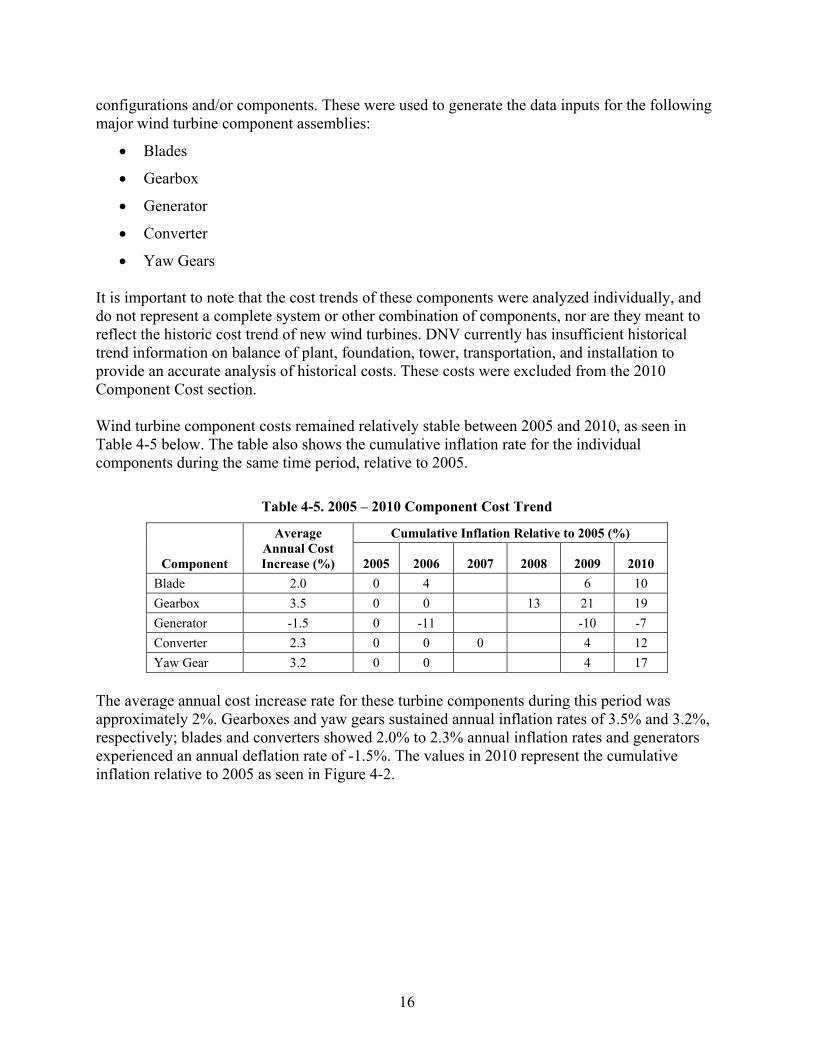
• Yaw Gears It is important to note that the cost trends of these components were analyzed individually, and do not represent a complete system or other combination of components, nor are they meant to reflect the historic cost trend of new wind turbines. DNV currently has insufficient historical trend information on balance of plant, foundation, tower, transportation, and installation to provide an accurate analysis of historical costs. These costs were excluded from the 2010 Component Cost section. Wind turbine component costs remained relatively stable between 2005 and 2010, as seen in Table 4-5 below. The table also shows the cumulative inflation rate for the individual components during the same time period, relative to 2005.

Table 4-5. 2005 – 2010 Component Cost Trend

Component

Average Annual Cost Increase (%)

Cumulative Inflation Relative to 2005 (%)

2005 2006 2007 2008 2009 2010 Blade 2.0 0 4 6 10 Gearbox 3.5 0 0 13 21 19 Generator -1.5 0 -11 -10 -7 Converter 2.3 0 0 0 4 12 Yaw Gear 3.2 0 0 4 17

The average annual cost increase rate for these turbine components during this period was approximately 2%. Gearboxes and yaw gears sustained annual inflation rates of 3.5% and 3.2%, respectively; blades and converters showed 2.0% to 2.3% annual inflation rates and generators experienced an annual deflation rate of -1.5%. The values in 2010 represent the cumulative inflation relative to 2005 as seen in Figure 4-2.

17

Cumulative Inflation Rate 2005 - 2010

-10%

-5%

0%

5%

10%

15%

20%

25%

Turbine Components

Com

poun

ded

Varia

nce

Blade Gearbox Generator Converter Yaw Gear

Figure 4-2. Cumulative Inflation Rate 2005 – 2010

5 PROJECT FINANCING

This section provides a high-level description of representative financing structures in 2010 and 2011 and relevant metrics for utility-scale wind power projects. Included is a qualitative outline of general wind development market conditions, including financing structures, capital availability, sources of funds (debt versus equity), and other information.

5.1 Financing Structures Wind projects typically require higher capital costs and lower operating costs than fossil-fueled power plants. These result in the need for higher levels of capital earlier than for a similar-sized conventional power project. As a result of the high capital cost for commercial-scale wind energy projects, the wind industry may use any one of eight primary financing structures and leasing options to manage project risk. The eight structures range in complexity and involve varying combinations of cash and tax equity capital from project developers and institutional investors, as well as commercial debt. These structures, outlined below, consider the differing financial capacities and business objectives of wind project developers, and the varying investment risk tolerances and objectives of the tax-oriented investors and debt providers. The descriptions of the structures below are based on the report, Wind Project Financing Structures: A Review & Comparative Analysis, by Harper et al. [3]. DNV has updated the prevalence of the various structures based on our knowledge of 2010 and 2011 market activities, when possible. Corporate Equity: In this structure, a single developer/investor (parent), with significant financial strength, will establish a special purpose entity to hold the assets of the project. Capital

18

initially generated from other projects and activities is used to fund the project. The project’s net cash flow and tax benefits flow back to the parent. While the parent performs sole management duties, other entities may take part in the day-to-day operational and maintenance responsibilities. [3] The Corporate Equity Structure is the simplest financing arrangement considered here, and is prevalent among larger developers and utilities that have the capacity to self finance. All financial and management issues are solved in-house, without requiring the approval of outside investors and all benefits flow directly to the parent. The parent may gain competitive advantage due to the flexibility and time-efficiencies inherent to this structure [3]; however, there are relatively few organizations active in the wind industry in 2011 with the capital resources to adopt this approach. Strategic Investor Flip: In the Strategic Investor Flip structure, an investor (known as a tax investor) interested in playing an active role in wind projects will negotiate a percentage ownership share with a project developer. This structure is similar to traditional joint ventures, but with three differentiating characteristics. [3] First, in the Strategic Investor Flip structure, the tax investor provides almost all of the project equity and, in return, is allotted almost all of the distributable cash and tax benefits. For example, a tax investor may provide an undercapitalized developer with 99% of the project’s total cost, leaving just 1% to be funded by the developer. In some cases, a tax investor has provided as much as 99.9% of the total project’s costs. [3] Second, at a point in time known as the flip point, the tax benefits and cash flow change typically in favor of the developer. The flip point occurs when a pre-negotiated internal rate of return (IRR) is met by the investor. It is often projected to be reached shortly after the tenth anniversary of the project’s commercial operation date, coinciding with the expiration of production tax credits (PTC) for the project. This strategy is favored by developers who are unable to efficiently use tax benefits. It is even possible to incorporate a second flip point, having the inversion of percentage allocations staged across two flip points. [3] Third, there is often an option included in the financial structure that allows the developer to purchase the tax investor’s ownership share after the flip point. By this time, tax benefits have been realized by the tax investor and the investment is recorded as a true equity investment. [3] The Strategic Investor Flip is less common today. This structure attracts third-parties who have equity to initiate projects to capture tax benefits, while allowing developers to retain some financial interest in the project. Institutional Investor Flip: Similar to the Strategic Investor Flip structure, the Institutional Investor Flip structure has developers bring in a separate tax investor who receives the project’s tax benefits. There is a flip point when the allocation of cash and tax benefits change. But there are important differences between these two flip structures. [3]

19

First, the Institutional Investor Flip structure tends to attract equity from more passive institutional investors that are not actively involved in the wind project. Second, the cash and tax benefit percentages received by the investor do not equal their initial investment percentage. This allows developers, who have a greater portion of initial equity capital invested in the project, to receive distributable cash from the project until they recover their investment, minus any tax benefits (which go to the institutional investor). The developer may receive what they have invested in the project, but not any returns on their investment, usually for the first four to six years of commercial operation. Once the developer has received 100% of their initial investment, 100% of the distributable cash plus tax benefits are allocated to the institutional investor until the flip point is reached. [3] Under the Institutional Investor Flip structure, the developer maintains management control over project operations, but the institutional investor has voting rights and veto power on major decisions. Developers who have capital to invest, but lack the ability to use tax benefits, find this structure appealing. Investors who want developers more vested in the success of the project also find this structure appealing. [3] This structure was popular for most of the 2000s. Repeated use has made investors comfortable with the structure and has brought improved standardization of transaction documentation. Pay-As-You-Go (PAYGO): Structurally, PAYGO is based on the Strategic Investor Flip, but with significant differences. Under PAYGO, the developer contributes roughly half of the initial capital required for the project, but the pre-“flip” cash and tax benefits do not match the percentage of equity contributions. In addition to their initial investment obligation, the tax investor makes annual payments based on the value of PTCs, allowing them to defer a portion of their equity investment over time. [3] PAYGO is typically used as a refinancing strategy by developers who are also major investors. This structure allows developers to reduce their investment stake in projects or raise capital for other corporate purposes. Additionally, developers with capital to invest can maintain an ownership stake in projects for a longer term than some of the previous structures. Investors lacking a tax appetite and, when unsure about PTCs, they tend to choose PAYGO to acquire existing wind project assets and tap tax investor capital to finance a portion of the acquisition costs. PAYGO allows tax investors to offset some of the risk associated with potentially lower-than-expected wind resource, new turbine technologies, and other project risks. [3] Cash Leveraged: In the Cash Leveraged structure, project-level loans are sized to be repaid from the cash flow generated by the project and secured by the project’s assets. Initial funding contributions by investors and developers are similar to those in the Strategic Investor structure, but the amount of initial equity capital required is reduced based on the amount of debt incurred. As a result, loan principal and interest payments decrease the amount of distributable cash available to the project’s investors. Debt can vary based on project requirements, but it is typically 40-60% of the total project costs. [3] By seeking limited recourse project debt, equity returns can increase and required equity contributions can decrease. By adding debt to the project, equity returns go up because debt is usually cheaper than equity. In general, investors are not comfortable contending with a lender

20

when the project encounters financial stress or if the project experiences foreclosure. As a result, more passive investors, like institutional investors not strategic investors, are usually sought out for this type of financial structure. The use of Cash Leveraged structures has increased significantly in 2010 and 2011 with the availability of the cash grant form of the Investment Tax Credit (ITC). Cash and PTC Leveraged: The cash and PTC-leveraged structure adds an additional layer of debt based on the expected PTC at the project level, and lasts the full term of the PTC loan – ten years. Both PTC-based and cash-based loans are secured by project assets and assignments of contract rights. PTCs are used as a tax credit for project owners and do not generate cash that is used to repay project-level debt. As a result, additional debt may negatively impact (possibly exceed) cash flow created by the debt service coverage ratio for the cash-based loan. Consequently, tax investors usually need to commit periodic additional equity investments into the project to address lender concerns. This is capped at the amount the PTC generated during that same period. [3] The same rationale for using debt to finance projects can be applied in this case. Lower costs associated with debt capital increase project equity returns while requiring less up-front investment. Developers favoring this structure are comfortable using debt to leverage their equity investment and believe the increase in IRR from incremental PTC debt justifies the added complexity. Maintaining control of projects also is attractive to developers and they usually already have experience in debt financing. By including the PTC, the number of tax investors may be limited because investors have to be willing to assume a contingent obligation around future capital contributions. [3] Due to the uncertainty associated with the future cost of capital for up to ten years, and the increased risk presented by a senior debt’s priority in receiving payments from the project, tax investors have been reluctant to participate in the Cash and PTC Leveraged structure and generally charge an associated premium when debt is used at the project level. Back Leveraged: Similar to the Institutional Flip structure, the Back Leveraged structure adds a layer of debt for the developer outside of the project, specifically at the holding company level. The developer initially shows interest in the project by acquiring debt to fund capital contributions. The debt provider can impact returns at the developer level, demanding a pledge of the developer’s equity interests, but the creditor has no recourse to the project company. Therefore, this structure does not affect project-level economics. The underlying allocations and structure remain the same as in the Institutional Investor Flip structure; however, loan terms are typically shorter (e.g., five years). [3] The developer can increase IRR by securing lower cost capital to fund initial contributions under this structure. It also can increase an undercapitalized developer’s equity participation. Since the financing is done at the developer level, tax investors are not impacted by this type of financial structure. The back leveraged structure is becoming more common because 1) it allows developers to increase their returns from projects through the use of leverage, and 2) tax investors are not exposed to project-level debt. [3]

21

Sale-Leaseback: The Sale-Leaseback is a recent innovation in wind project financing [4]. It became more viable when the PTCs were supplemented with the ITCs and cash grants; both can be used by a non-operating owner. The Sale-Leaseback provides benefits unavailable in the other structures and allows the borrower to obtain 100% financing. Equity investors have a starting tax basis equal to the acquisition price of the project, which can be beneficial in calculating tax benefits, including incentives and depreciation. The Sale-Leaseback structure can provide access to capital from bank leasing companies, which may be unavailable in an Investor Flip structure. Either the lessee or the lessor has the option to apply for the grant. The lessee can apply for, and be the recipient of, the grant; the lessee places the property in service, sells the property to the lessor, and leases it back within three months of the project being placed in service.

5.2 Capital Availability and Cost of Capital According to several discussions with equipment manufacturers, developers, and representatives of finance institutions, availability of project financing was one of the significant limiting factors in the U.S. wind energy market in 2009 and early in 2010, but the situation has since rebounded significantly. The primary reason for project financing limitations was the economic downturn that hit the U.S. and global economies in the fall of 2008, and led to a tightening of the financial markets. The global credit crisis negatively affected wind project financing in two important ways:

• Project-level debt – In the aftermath of the credit crisis, lenders were sizing debt on more stringent terms compared to pre-crisis conditions. This resulted in increased borrowing costs and an overall reduction in the level of lending for new projects in 2009 and early 2010. The availability of project-level debt has since rebounded significantly.

• Tax equity – Historically, most projects relied largely on tax equity investment for project financing. The number of tax equity participants and the associated availability of tax equity were significantly reduced due to commensurate reductions in corporate profits and the resulting tax appetite. About 20 investors were active in the renewable energy tax equity market before the crisis, but this was reduced to a handful of organizations by the end of 2008. The number of investors active in the market rebounded, but as of 2010, it was still below the pre-crisis level at about 16 tax equity investors. All were not active in the U.S. wind market [5]. The need for tax equity was decreased by the use of the cash grant program instead of the ITC and PTC programs.

In an effort to counteract the impact of the global credit crisis on the wind industry, provisions were included in the American Reinvestment and Recovery Act (ARRA) passed in February 2009. This included the aforementioned cash grant in lieu of the ITC. This incentive provided financing for projects that otherwise would have had difficulty monetizing the tax benefits associated with the PTC or ITC due to the limited availability of tax appetite. The U.S. Treasury disbursed $1.4 billion in 2009 and $3.5 billion in 2010 to wind projects under this program [6]. Prior to the global credit crisis, the cost of project-level debt was trending upward. During this period, commonly referenced benchmark rates were relatively high, while bank margins were

22

relatively low, ranging from about 125 to 175 basis points. As a result of the credit crisis, base rates dropped significantly, but margins increased to about 325 to 375 basis points. The combined result is that the overall interest rates for project-level debt have remained fairly steady in 2010 and 2011, with perhaps a slight reduction in interest rates relative to pre-crisis levels. Bank margins have come down recently from around 275 to 300 basis points. [7]

5.3 Empirical Findings on Financial Metrics DNV conducted empirical research on various financial metrics including the following standard financial metrics:

• Cost of standard equity – defined as the 20 year after-tax internal rate of return (IRR) for the primary project owner.

• Cost of tax equity – defined as the 20 year after-tax IRR for a tax equity owner. In projects with a flip structure, this includes both pre- and post-flip cash flows.

• Cost of debt – defined as the before-tax all-in annual interest rate for a term loan. This does not include construction loans, which are typically short-term instruments.

• Debt fraction – defined as the percentage of the overall project cost that is funded by a term loan. This does not include any construction loan.

• Debt tenor – defined as the length of the term loan in years.

• Debt service coverage ratio (DSCR) – defined as the coverage ratio for sizing debt using a P50 production case. In practice, most term loans are also sized on the one year P99 production case, with a DSCR of 1.0. Lenders may offer the smaller of the loan sizes between the two cases. [8]

DNV reviewed project-level pro formas for 15 projects developed in 2010 and 2011. Most of these projects were funded using the cash-grant version of the ITC. DNV reviewed recent public presentations and reports from debt and equity institutions to gather information on target rates of return. DNV also interviewed six project participants, between June 2011 and July 2011, including project lenders, sponsors, and equity investors to discuss our empirical findings. The results below reflect both the empirical data from the evaluated pro formas and the results of interviews with project participants. Where appropriate, a range of results is presented. However, individual projects may vary materially from the ranges indicated below. The cost of standard equity ranged from 8% to 13%, with a baseline of 10%. This was lower if an equity holder were buying into an equity stake in an operating portfolio as compared to early-stage, non-operating development portfolio. The cost of tax equity ranged between 7% and 15%, with a baseline of 9% or 12% depending on the presence or absence of senior debt (e.g., a term loan). There were relatively fewer tax equity deals in years when the cash grant was in place. There was a premium of approximately 300 basis points (3%) on the cost of tax equity, if the project had senior term debt. This market was much more variable and project-specific than the debt market and was influenced by dynamics in the affordable housing market, which competes with renewable energy projects for tax equity

23

investment funding. DNV’s review of this metric relied more heavily on discussion with industry partners than our review of the debt-related metrics. The cost of debt ranged between 6.75% and 8%, with a baseline of 7.125%. The typical bank margin over LIBOR was approximately 225-325 basis points. In 2010 and 2011, many term loans were fully amortized over longer periods (e.g., 15-18 years) as opposed to mini-perm structures that included a large balloon payment after 5 to 7 years. Mini-perm structures were more common in late 2008 and 2009 following the financial crisis of 2008. Other findings included the following:

• The debt fraction ranged between 40% and 55%, with a baseline of 45%, though some isolated cases were identified outside this range,

• The debt tenor ranged from 15 to 18 years, with a baseline of 17 years, though some isolated cases were identified outside this range, and

• The base case DSCR ranged from 1.4 to 1.55, with a baseline of 1.45.

Overall, the debt market appeared to be more consistent across projects than the tax equity market, which had more project-specific details. Our investigation converged quickly on the debt numbers and there were fewer comments on these in our discussions with industry partners.

24

6 REFERENCES

[1] Poore, R. Development of an Operations and Maintenance Cost Model to Identify Cost of Energy Savings for Low Wind Speed Turbines: July 2, 2004 -- June 30, 2008. NREL/SR-500-40581. Work performed by Global Energy Concepts, LLC, Seattle, Washington, Golden, CO: National Renewable Energy Laboratory, January 2008. http://www.nrel.gov/docs/fy08osti/40581.pdf [2] American Wind Energy Association. U.S. Wind Industry Annual Market Report Year Ending 2010. Washington D.C., 2011. http://www.awea.org/learnabout/publications/reports/AWEA-US-Wind-Industry-Market-Reports.cfm [3] Harper, J.; Karcher, M.; Bolinger, M. Wind Project Financing Structures: A Review & Comparative Analysis. LBNL-63434. Berkeley, CA: Lawrence Berkeley National Laboratory, September 2007. http://eetd.lbl.gov/ea/emp/reports/63434.pdf [4] Bolinger, M. Community Wind: Once Again Pushing the Envelope of Project Finance. LBNL-4193E. Berkeley, CA: Lawrence Berkeley National Laboratory, January 2011. http://eetd.lbl.gov/ea/emp/reports/lbnl-4193e.pdf [5] Partnership for Renewable Energy Finance. Prospective 2010-2012 Tax Market Observations, 2010. http://uspref.org/white-papers [6] “Section 1603: List of Awards.” Microsoft Excel file, U.S. Department of Treasury. http://www.treasury.gov/initiatives/recovery/Documents/Web Posting.xlsx [7] GlobalData. Project Finance Trends in the Global Wind Energy Market to 2015 - Deals, Competitive Analysis of Debt Providers, Advisors, Sponsors and Interest Rates, August 2010. [8] Lowder, T. P50? P90? Exceedance Probabilities Demystified. Renewable Energy Project Finance. Golden, CO: National Renewable Energy Laboratory, October 2011. https://financere.nrel.gov/finance/content/p50-p90-exceedance-probabilities-demystified.

A-1

APPENDIX A – FAILURE RATE AND PARTS COST ASSUMPTIONS Table A-1. Reference Scenario Failure Rates and Part Cost Assumptions

System Component Failure

Prediction

Failures per 100 parts by

Year 20

Weibull Curve

Parameter – Alpha

Weibull Curve

Parameter – Beta

Parts per Turbine

Parts Cost ($) Crane?

Parts in Project

Failures in 20 Years

Rotor

Blade-struct. Repair Constant Rate 5.0 3 87,500 YES 300 15

Blade-nonstruct. Repair Constant Rate 20.0 3 3,000 NO 300 60

Pitch cylinder & linkage Weibull Curve 10.0 3.5 3 3,800 NO 300 547

Pitch bearing Weibull Curve 50.0 3.5 3 13,100 YES 300 13

Pump & hydraulics Weibull Curve 12.0 3.5 1 2,200 NO 100 142

Pitch position xdcr Weibull Curve 12.0 2.0 3 1,800 NO 300 468

Pitch motor Weibull Curve 15.0 1.1 0 8,400 NO 0

Pitch gear Weibull Curve 12.0 3.5 0 4,600 NO 0

Drive Train

Main bearing Weibull Curve 39.0 3.5 1 24,400 YES 100 10

High-speed coupling Weibull Curve 25.0 3.5 1 6,700 NO 100 39

Gearbox and Lube

Gearbox-gears & bearings Constant Rate 5.0 1 154,700 YES 100 5

Gearbox-bearings, all Constant Rate 5.0 26.0 3.5 1 800 YES 100 35

Gearbox-high speed only Weibull Curve 26.0 3.5 1 36,700 NO 100 35

Lube pumps Weibull Curve 12.0 3.0 2 2,400 NO 200 294

Gearbox cool. fan motor Weibull Curve 19.0 1.1 2 2,000 NO 500 195

Generator and Cooling

Generator-rotor & bearings Constant Rate 10.0 1 91,600 YES 100 10

Generator--bearings only Weibull Curve 17.0 3.5 2 2,100 NO 200 184

Full converter Weibull Curve 15.0 2.0 1 9,500 NO 100 117

Gener. cooling fan motor Weibull Curve 19.0 1.1 1 1,600 NO 100 98

Contactor, generator Weibull Curve 20.0 2.0 3 13,500 NO 300 235

Partial converter Weibull Curve 15.0 2.0 0 2,600 NO - -

A-2

System Component Failure

Prediction

Failures per 100 parts by

Year 20

Weibull Curve

Parameter – Alpha

Weibull Curve

Parameter – Beta

Parts per Turbine

Parts Cost ($) Crane?

Parts in Project

Failures in 20 Years

Brakes and Hydraulics

Brake caliper Weibull Curve 10.0 2.0 1 700 NO 100 194

Brake pads Constant Rate 200.0 10.0 2.0 1 5,900 NO 100 200

Accumulator Weibull Curve 6.0 3.0 4 1,500 NO 400 1,356

Hydraulic pump Weibull Curve 12.0 3.0 1 4,900 NO 100 146

Yaw System

Yaw gear (drive+motor) Constant Rate 5.0 4 6,000 NO 400 20

Yaw motor (with brake) Weibull Curve 10.0 2.0 4 2,400 NO 400 776

Yaw sliding pads Weibull Curve 10.0 3.5 8 800 NO 800 1,462

Control System

Control board, top Weibull Curve 15.0 2.0 1 5,500 NO 100 117

Control board, main Weibull Curve 15.0 2.0 1 8,600 NO 100 117

Control module Weibull Curve 15.0 2.0 13 6,100 NO 1300 1526

Sensor, static Weibull Curve 14.0 2.0 17 500 NO 1700 2184

Electrical and Grid

Main contactor Weibull Curve 20.0 2.0 1 9,200 NO 100 77

Main circuit breaker Weibull Curve 30.0 2.0 1 10,800 NO 100 7737

Soft starter Weibull Curve 30.0 2.0 0 700 NO - -

Misc. (All others)

Miscellaneous parts Constant Rate 5.0 1 100,900 NO 100 5

B-1

APPENDIX B – SCENARIO RESULTS Table B-1. All Scenario Model Results – O&M Costs by Project Operating Year

O&M Cost by Project Operating Year ($/turbine/year) Year 1 2 3 4 5 6 7 8 9 10 11 12 13 14 15 16 17 18 19 20

Reference Scenario 24,300 26,300 28,900 31,300 34,200 36,500 38,900 41,000 42,700 44,600 46,200 47,300 47,400 47,700 48,500 49,000 49,700 50,900 51,300 51,300

High Failure Rate Scenario – Blades

26,900 29,000 31,600 34,000 36,800 39,200 41,500 43,700 45,400 46,300 47,700 47,900 48,300 49,300 49,400 50,600 51,300 51,900 52,400 52,900

High Failure Rate Scenario – Generator

26,400 28,500 31,000 33,400 36,300 38,700 41,000 43,100 44,800 46,800 47,200 48,200 48,400 48,700 49,500 50,100 50,800 51,900 52,400 52,400

High Failure Rate Scenario – Gearbox

26,000 28,000 30,600 33,000 35,900 38,300 40,600 42,700 44,400 46,400 47,900 47,900 48,100 49,200 49,200 50,400 51,000 51,600 52,100 52,600

100% Replacement Scenario – Blades

41,200 43,300 45,800 48,200 50,800 53,100 54,900 56,700 58,100 59,400 60,400 60,900 61,500 62,100 62,400 63,300 64,100 64,800 65,600 65,800

100% Replacement Scenario – Gearboxes

37,900 40,000 42,500 44,900 46,800 49,200 51,300 53,200 54,100 55,700 56,300 57,100 57,300 57,700 58,300 58,900 59,600 60,600 61,100 61,200

100% Replacement Scenario – Generators

32,000 34,000 36,600 39,000 41,700 43,400 45,600 47,500 49,100 50,200 51,400 51,700 52,000 52,900 53,100 54,200 54,900 55,500 56,100 56,500

Serial Replacement Scenario – Blades

22,900 25,000 27,600 132,900 135,700 138,100 37,500 39,600 41,300 43,300 44,800 46,000 47,200 47,300 47,400 48,600 49,200 49,800 50,800 50,800

Serial Replacement – Gearboxes

23,400 25,500 28,000 103,700 106,600 109,000 38,000 40,100 41,800 43,800 45,300 46,400 46,600 46,900 47,800 48,300 49,000 50,200 50,600 50,700

Serial Replacement – Generators

23,200 25,200 27,800 73,500 76,300 78,700 37,800 39,900 41,600 43,600 45,100 46,200 46,400 47,600 47,600 48,900 49,500 50,000 50,500 51,000