DATA BUS NETWORK SIMULATION

IBM FEDERAL SYSTEMS DIVISION

PREPARED FOR

AIR FORCE AVIONICS LABORATORY

U.S. DCPMTMENT OF COMMERCE NatioMl Ttdmical lirtomiat«« Service

AD-A025 115

MARCH 1976

Best Available

Copy

MCMMTV ct***iFir*T}0* nr fWtttm r>mim pm»**»m

REPORT DOCUMENTATION PAGE READ IMSTHtTTiriNS BEFOIIC COMPLF.TINf, FORM

AFAL-TR-7 5-109

1 60VT «CCtUlO« HO I ■Ctl»ltMT-t C*T«LOC MUM*f ■

DATA BIS NETWORK SIMTLATION

t TT^t O» Hf^OIIT • ■ ■ •■ ,0 covtato Tntcria 31 Mar. 197S - 11 Aug. 1975

• »caroMMMC oac ataoar Mu«Ma 76W-0026

T auTMONro

L. Balliet J. W. Dalton, J. R. Earl, W. W. Scott 75-C-1133

a*MT Huaacafu

K rtaroMMiac oao*Mii*TioN H*itc SMÜBSSM

IBM Corporation ISO Sparkaan Drive Huntavllle, AL 35805

i« »aocaau CLCHCMT aaojtCT T.I« «at* • aoa« uaiT NüMacat

Project 2052 0303

n. coNTnoLLiac orncc MMMI »NO «ooacst

Air Force Avionics Laboratory Wrigh«- Patterson AFB, Ohio

it ataoar OATC

March 1976 11 MuM*ca of a*6ts

£L I« MONlToaiNC MittCV MBM • «OOaESVl' mtltml Ifam Cmtlrtllmi Olt'ct) IS SCCuaiTT CL»SJ (ml tKlt 'mptrll

Unclassified HS OCCLAMl'ICATION 0OaMCa4DlMC

KMlDukC

nSTIHSWTION tTATCMCMT (ol Ihlm ••

Approved for puolic release; distribution unlimited.

IT. nSTMISUTIOH tTATCHIMT (ol Ittt mtmftmcl m>fn* In SI»« JO. II milfttl Irmm ftaaartj

is «oaatcneaTABY HOT»

IS. RCV aoaOS (SmUmm an <»«>»•• •<<• •' n»t»tmir m* Hmflh »» Mac» >

Data Bus Simulator Transmission Line MIL-STD-1553 Multiplex

AMTMACI fC—W—« an ravarw •!«• (I ■Mnmatr «a^ l«m«l|i *r Mac» »aaitirj

This report describes a FORTRAN coded digital computer simulator program for predicting waveforms on a data bus network consisting of a main bus with numerous stubs connected via transformer couplers. Bus operation is at baseband with configurations compatible with MIL-STD-1553. The report includes simulation theory, program operation, operating instructions and laboratory verification data. ._

mas suutcrn atwi POMM

• JAM n 1473 EOITIOM OF I MOV •■ IS OSSOLETC

//

UNCLASSIFIED MCUMITV CLUMFICaTIOM OF TMIS a «Of rMkaa Oala iMara«

FOREWORD

This report describes a simulation program and related verification

hardware developed for the Air Force Avionics Laboratory by the IBM

Corporation, Huntsville, Alabama. This six month effort was performed

under Contract F33615-75-C-1133 and Work Unit 20520303. MIL-STn-1553A

data networks are simulated using iterative time domain calculations

and results verified with breadboard hardware. Correlation of

simulation results with hardware is excellent and modelling improvements

are presented for skin effects, transformer coupling and timing.

The results suranarized in this report were obtained by Bud Balliet,

Program Director, Jamt., W. Dalton, William W. Scott and James R. Farl.

Michael J. O'Connor was the contract monitor for the Air Force Avionics

Laboratory.

^it y m

•nit t:ii.M/^3 ■MWNCrS MTIFiMTtBX

IT »[«IKiWTIO!1 l«tttt!Lmi «J£S

" JWT in... J . M •■,: uT

P ili

TABLE OF CONTENTS

Section Title Page

I Introduction 1

II Theory 4

A. Transmission Line Simulation 4 B. Reflections 14 C. Stub Simulation 16 D. Transformer Modeling 19 E. Suamary of Theoretical Approach and Assumptions 28

III Program 30

30 30

30 30 30 4] 41

IV Simulation Operation 47

A. DEC-10 Compablllty 47 B. Input Data 47

1. Input Definitions 48 2. Array Inputs 50

C. Constraints of the Simulation 50 D. Coupler/Stub Calibration Discussion 51

V Laboratory Evaluation 53

A. Data Bus Breadboard 53 B. Test Data 58

VI Conclusions and Recommendations 69

References 70

A. Organization B. Basic Routines

1. Main Routine 2. Subroutine Filter 3. Subroutine Plotter 4. Subroutine SAVPNT 5. Subroutine PL4020

IV

LIST OF ILLUSTRATIONS

Figure

1 2 3

5 6 7

8 9

10

11 12 13 14 15 16 17« 17b 18 19 20 21 22 23 24 25 26 27 28 29 30 31 32

33 34 35 36 37 38 39 40

Title

Simulator Element» Transforaer Coupler Scheaatic Possible Equivalent Circuit of a Transmission Line Line Characteristics Response of Sample Cable to a Unit Step Input Line Response to Step Input Skin Effect Line Simulation Algorithm (Ignoring Time Delay) References for Estimating Function Reflection Signals at Bus/Coupler Junction Average Energy Spectral Density for MIL-STD-1553 Symetrical Waveforms Output Response to Transformer 11 Transformer and Stub Line Equivalent Circuit Equivalent Circuit from Stub to Main Bus TRANS2 Test Setup Output Response to TRANS2 Block Diagram of Data Bus Cable Simulation Main Subroutine (Sheet one of two) Main Subroutine (Sheet two of two) Filter Subroutines Decimal Codes Subroutine Floter (Key-1) Subroutine Floter (Key-2) Subroutine Floter (Key>4) SAVFNT PL4020 Flow FLTEND Flow FLOTID Flow Coupler Box Breadboard Driver Schematic Breadboard Driver Input and Output Waveforms Setup A Setup B Simulator/Lab Comparison for 120 Feet of Cable into 68 ohms Simulator/Lab Comparison for one 10 Foot Stub Simulator/Lab Cooparlson for one 20 Foot Stub Simulator/Lab Comparison for eight 10 Foot Stubs Simulator/Lab Comparison for eight 10 Foot Stubs Simulator/Lab Comparison Driving Stub #1 Simulator/Lab Comparison at Stubs #1 and #8 Simulator/Lab Comparison for one 20 Foot Stub Simulator/Lab Comparison for eight 10 Foot Stubs

Fate

2 3 5 8 9

10

12 13 13

18 21 22Figure 13. 24 26 26 31 32 33 34 37 38 39 40 42 44 45 46 54 56 57 59 59

60 61 62 63 64 65 66 67 68

LIST OF TABLES

Table Title Page

1 Line Algorithm Suimnary 15

2 Reactance and Corresponding Capacitance 19 presented by Ten and Twenty Foot Lossless Stubs Terminated in an Open

VI

SUMMARY

The widespread application of baseband data buses for avionics system Inter- face has obrlated the importance of computer simulation for design and evaluation of complex cable networks. This report describes a general purpose digital computer program that provides this capability. Programming routines are coded in FORTRAN IV for easy modification and for operation on either an IBM System 370 or a Digital Equipment Corporation DEC 10 computer. The simulator is specifically designed to emulate one megabit MIL STD 1353 type waveforms and bus configurations.

A typical MIL STD 1553 data bus consi; ts of a main bus accessed through shorter cables, herein called stubs. These stubs present a capacltive load to the bus coupler which is located at ehe main bus, stub junction. Coupler trans- formers with their stub loads are simulated as second order systems with parameters derived from measurement data. Tustlns transformation is used to produce different equations that permit time domain computation. Itera- tive time domain calculations are employed. Reflection coefficients are used to calculate signal imperfections caused by junction and termination dis- continuities. Transmission line filter effects are acconmodated by an independent algorithm that takes skin effects into account. Procedures are Included for operating the program and for characterizing the line and the transformer couplers from laboratory data. The program will permit stubs of lengths up to nominally 20 feet at numerous points along the main bus trunk. Multiple stubs can also be simulated so that the amount of stub loading is not bounded.

To verify validity of simulation, a breadboard of a typical bus network was constructed. This breadboard permitted a worst case configuration of a 300 foot main bus trunk with 8 stubs connected via either of two types of trans- former couplers. Results produced by the simulation agreed favorably with data taken on the breadboard. Additional transformer/stub characterization study is recommended to better correlate transformer parameters to the software model.

vii

I. INTRODUCTION

The class of data bus defined by MIL-STD-1353 (reference 1) employs time division multiplexing at baseband with a unique synchronization waveform followed by Biphase L (Manchester II) coded binary data. The main bus trunk can be accessed by as many as 33 cable stubs. A data bus system thus represents a complex network for simulation.

Network simulation can generally be approached In either the time domain or frequency domain with each approach providing advantages and disadvan- tages. In general, time domain simulation will simplify handling complex waveforms and was the approach IBM selected during a Company-funded devel- opment in 1974. This development resulted in a FORTRAN coded simulation tool that emulated MIL-STD-1553 networks, but did not provide transformer coupling.

Recognizing the importance of a network simulation tool for continued MIL- STD-1Ü53 related network study, this contract was awarded to IBM by the Air Force Avionics Laboratory for supplying a modified version of IBM's original simulator. Modifications were to incorporate transformer coupling and add provisions for transmission line skin effects and other features to general- ly improve utilization flexibility.

Figure 1 shows the elements of the data bus network simulator. The cable of specific Interest is twisted shielded wire pair and is shown divided into line segments. The main trunk contains up to 30 segments each of identical length. For a maximum MIL-STD-1553 configuration, each line segment would be 10 feet long to simulate a 300 foot main trunk. At each line segment junction, stubs can optionally be connected through couplers. A coupler consists of a pair of isolation resistors and a transformer connected as shown in Figure 2 ■ Again referring to Figure 1 , each stub in turn also contains cables that terminate in a load R . R simulates the impedance of a receiver/transmitter. The ends of the main trunk are also terminated in an impedance R , normally but not necessarily equal to the characteristic impedance of the line.

Normally, one of the receiver/transmitters on a stub will be activated in the transmit mode. Thus, a generator, G, can be simulated to drive the bus from one of the bus stubs. It can also be connected to one of the ends of the main trunk. The generator produces a variable three-level format in- cluding a MIL-STD-1553 waveform to drive the bus from an off state (level 1) to a plus state (level 2) and/ot a minus state (level 3). The source impedance of the generator is set at a value that can differ from R or Z .

o

As noted in Figure 1 , N «tubs can be connected to a given Junction of the main bus. "N" can vary and can be any positive real integer. Two restrictions are placed on the use of multiple stubs at any Junction. These are that: 1) "N" must equal one if the generator is active through that specific Junction, and 2) all "N" stubs must be of the

' LINE NO. r

LINE NO. 2

TRANSFORMER COUPLER

LINE NO. 3

■^ S-

TRANSFORMER COUPLER

N STUBS

LINE NO. 3

TRANSFORMER COUPLER

7 STUB LOAD

•ANY LENGTH UP TO 30 FEET

M * 1,1,9 STUBS AT EACH JUNC'ON

G■GENERATOR

RT ■ TERMINATION RESISTANCE

RL = LOAD RESISTANCE

Figure 1. Simulator Elements

MAIN TRUNK

TMSTED SHIELDED PAIR LINE

MAIN TRUNK

STUB

Figure 2. Transfomer Coupler Schematic

same length tor all active 1 unctions. Thus, the number of stub loads that can be simulated Is not bounded.

The report Is organized to first cover basic theory of network simulation. This Is provided In Section II and Includes the treatment of the transmission line, couplers and junction calculations. Section III describes the basic program organization and relates the theory to program routines. With an understanding of the program. Section IV provides operation instructions and describes operational capability and limitations. Section V describes the breadboard used in the simulator development and documents test data. The final section briefly provides conclusions of the development program.

II. THEORY

Thli section describes the basic data bus elements to be simulated and pro- vides the theoretical basis for the simulation.

A. TRANSMISSION LINE SIMULATION

Each of the transmission line segments Identified In Figure 1 will modify the signals passing up and down the data bus. The task of the transmission line simulation Is to accurately duplicate the transfer characteristics of a selected line via a set of parameters that accurately describe it. It is furthermore highly desirable to use parameters that are easily obtained by laboratory measurement.

1. Applicable Line Parameters

Transmission line theory is well documented (see References 2, 3, and 4 for specific examples)*. Most treatments start by modeling the dis- tributed properties of a length, I , by equivalent Rs, L and C as shown in Figure 3 . The resistance, inductance and capacitance is defined per unit length. From this model idealized transfer equations and key line characteristics are readily derived. For a line free of reflection (infinite length or uniquely terminated), it is shown as a function of frequency, that.

out

in e-Y* (1)

whereY is the propagation function.

Y((D) -^(R + jwL)(G + juC)

In terms of real and imaginary components,

Y(a)) - a(u) + jS(u))

(2)

(3)

a is the attenuation tern and Is a function of frequency. 0 is the delay or phase term and also frequency dependent. In well behaved lines (non dispersive) ß is linear with frequency and merely represents a constant time delay, !£,, in the time domain.

*Unless specifically noted otherwise, transmission line equations used in this report were all fully developed in these references.

IRt • wwv

IL

Ic R. "^G

^ • length of line

Figure 3. Possible Equivalent Circuit of a ^-..«w-'ssion Line

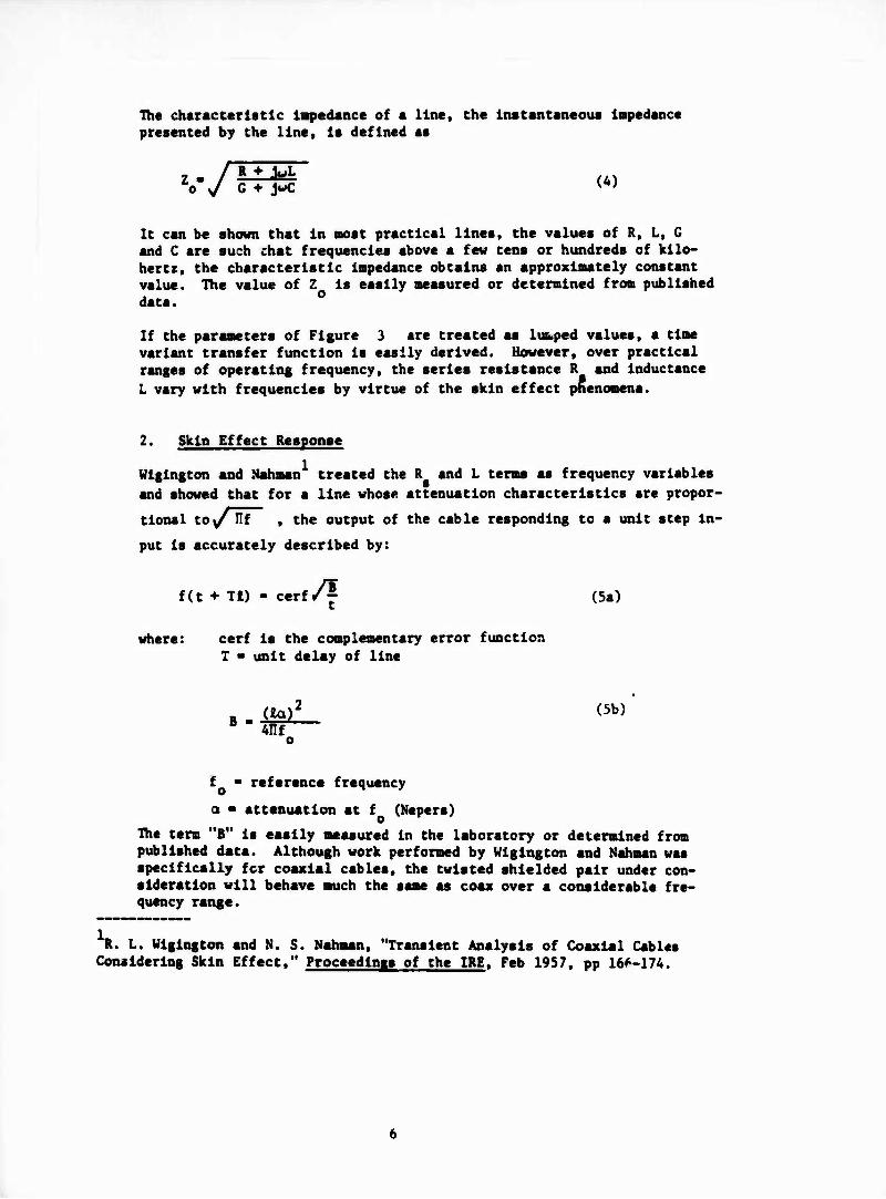
The characteristic Impedance of a line, the Instantaneous Impedance presented by the line. Is defined as

z. /TTJ^T © y G ♦ jwc w

It can be shown that In most practical lines, the values of R, L, G and C are such chat frequencies above a few tens or hundreds of kilo- hertz, the characteristic Impedance obtains an approximately constant value. The value of Z Is easily measured or determined from published data. 0

If the parameters of Figure 3 are treated as lumped values, a time variant transfer function Is easily derived. However, over practical ranges of operating frequency, the series resistance R and Inductance

L vary with frequencies by virtue of the skin effect phenomena.

2. Skin Effect Response

Wlglngton and Nahmen treated the R and L terns as frequency variables

and showed that for a line whose attenuation characteristics are propor-

tional to/Hf , the output of the cable responding to a unit step In-

put Is accurately described by:

A f(t + Tl) - cerf/^r (5a)

where: cerf Is the complementary error function T - unit delay of line

(la) 2 (5b)

AHf o

f - reference frequency

a • attenuation at f (Nepers)

The term "B" Is easily measured In the laboratory or determined from published data. Although work performed by Wlglngton and Nahmen was specifically fcr coaxial cables, the twisted shielded pair under con- sideration will behave much the same as coax over a considerable fre- quency range.

R. L. Wlglngton and N. S. Nahmen, "Transient Analysis of Coaxial Cables Conaidering Skin Effect," ProceedinRs of the IRE. Feb 1957, pp 16^-17A.

Figure 4 shows characteristics of the twisted shielded pair (TSP) used in the verification breadboard of a larger cable RG 108A/U. The region at higher frequency where the attenuation, a is linear with frequency on the log/log plot corresponds to the condition for compliance with equation(5). Thus, the saaple cables will reasonably respond in accordance with equation (5) at high frequency.

Figure 5 shows the tine response of the #24 Teflon TSP sample depicted in Figure 4. The theoretical curve is the response anticipated by equation (5) using a value for B derived from Figure 4. The fact that the actual response does not achieve an amplitude equal to the theoretical is attributed to the higher attentuation at lower frequency, i.e., deviation from the linear \/Wl region. The actual response tracts the theoretical closely along the edge of the input rise (region of high frequency).

3. Transmission Line Algorithm

In the simulation program, signals passing up and down the data bus are treated as incremental step functions. For a transmission line segment, an input step of amplitude "E" will produce an output v(t+T ). See Figure 6. During the region where equation (5) applies.

vCt-Wi) - E cerf /I (6)

This expression can be evaluated over the time Increments between t., t , t , t_, etc. where each increment is of identical duration and corresponds Co tne computation time of the program. Equation (6) for a single step becomes:

r(t+Tl) - E (cerf/|l 1 + cerf^ + cerf 4 (7)

For a given length of line and constant time increments, each evaluation will be constant and equation (7) is represented by:

v(t4Tl) • E(G1 + G2 + G3 + )

G , G,, G. etc are constants

(8)

FREQUENCY (MHZ)

100

10

CABLE LOSS VS.

FREQUENCY

(LOG/LOG)

u. 8 » o

1.0

J i : i i i i < j ( i t i » »i J i I LJJLU 0.1 1.0 10.0

FREQUENCY IN MEGAHERTZ

Figure 4. Line Characteristics

I

H to Uj

w B

g 8 I

v Oi 2

a- z O

M

a! g

u

fc

il M

w u 2 tj

"1 2S S

i Z M

It m o

\

\

•s 13 i I

M

«

I

01

Figure 6. tine Response to Step Input

10

An arbitrary signal Into a line segment can be treated as a sequence of snail step functions. This Is depicted in Figure 7. The signal f(t) Is shown being composed of superimposed step Inputs AE, occurring at t^, AE, at tj.AE. at t-, etc. From Figure 7, it can be seen that:

Vout " V El + G2 AE(1.1) + G3 AE(1.2) + (9)

where: 1 - present value

1-1 - first past value

1-2 ■ second past value, etc.

AE - amplitude of Incremental Input changes

The above expression Indicates that the present output is a function of the previous step Inputs. If the number of past input evaluations were made very large, ths evaluation would closely approach equation (6). Since this Is not practical or desirable, an estimating function is Introduced to allow the output to approach an attenuated value of the Input after a fixed number of past value calculations.

The estimating function calculation is referenced to Figure 8. It consists of the implementation of the differential equation for allowing the output to approach the input exponentially.

. ^- k[V-v(t)] (10)

In the diagram of Figure 9, the output after t is allowed to approach a final value at V., passing through V. at the t . The solution to the above Is simply: y

V - (V3-V1)(l-e't/T)

(11)

Evaluating the above at V - (Vj-V.)

- £n

t - t y , * (12)

3 2

VV

11

AE,

AE,

1- AE, 61 +AE1 G2 ♦AE, G3 +...

2 s A E2 G1 + A Ej Gj + A E3 G3 +

AE, 3-AE3G1+AE3G2+AE3G3

AE. 4- AE4G1+AE4G2 + .

AT TIME I,

'OUT «G^Ej ♦ G2AE(j.1) ♦ G3AE<i.2) ♦ + VM ,(A)

PRESENT VALUE

1ST PAST VALUE

2ND PAST VALUE

ESTIMATING PREVIOUS FUNCTION OUTPUT

TOTAL

Figure 7. Skin Effect Line Simulation Algorithm (Ignoring Time Delay)

12

T

TIME

Figure 8. References for Estlaating Function

AV IN

STUB

Ave

Figure 9. Reflection Signals at Bus/Coupler Junction

13

where the value for k ■ r ■ G.

The complete estimating function which takes the form of equation (10) is:

(W'-Va)" (13) where: E/J ox " 3rd past input

V,, -* - 3rd past output

G7 - attenuation tern for line

G4 « k factor discussed above

A transmission line is calibrated at some convenient length. This was arbitrarily set at 100 feet. From curves similar to that of Figure 5, values for 04 and 07 are determined. The value for 04 is set as the relative amplitude after 250 ns; the value of 07 is set as the relative amplitude after 1500 ns.

B. REFLECTIONS

As a wa-"front travels down the main bus it «rill encounter discontinues at each coupler Junction (and possibly at the end terminations). See Figure 9. Part of the incident wave, 4VR, „in be reflected and the other part, 4VT,

will continue in the direction of the original wave. A portion of the wave, JVg, will also travel down the stub. The reflection coefficient, , and transmission coefficient, , describe the amplitudes of these waves.

(14)

where z ■ instantaneous impedance seen at a junction

p - 1 + V

(15)

The line algorithm is summarized in Table 1. The change In subscript of Table 1, equation B as compared to that of equation A in Figure 7 takes the delay of a line segment into account. For example, the first term of equation A has an "1" index whereas the first tern of equation B is indexed "1-1". The delay of one line segment is one computation cycle as indicated by this indexing.

14

Table 1. LINE ALGORITHM SUMMARY

E - Inputs V - outputs 1 - present tins

outi

Where:

Gl ^(i-l) + G2 ^(1-2) + G3 ^(1-3) + (Ei-*G7 + V8-3) C4 + '«-»' ™

Gl"cerf,/ll c«) G2-cerf^f ^ (D)

G3 " Cerf^TT " cerf S£t W G7 • final relative amplitude for longest pulse,

determined at value after 1500 ns.

r. - li chosen to provide desired amplitude (F) ' " T * sfter 250 ns.

15

The Instantaneous Inpedance seen at a junction Is the parallel combination of the line, Zo, and the stub load.

Thus,

('o)(S)

0 * (16)

The Instantaneous signal amplitudes are as follows:

AVU - AV, v (17)

R In

AVT - L\in (l+v) (18)

AV • LV, il+X) i (TRANS 1) (19) s in

where (TRAN 1) Is the transfer function of the coupler as viewed from the bus side.

It is noted that - is a function of time making many of the dependent variables also functions of time. This point Is discussed later In the report.

In the simulation program the signal wavefronts, AV and AV are calculated

and their summations accumulated each cable junction. These se summations are used to reconstruct a composite waveform for display.

C. STUB SIMULATION

There were two approaches considered for stub simulation. The first, which was employed during the original simulator development, is to calcv'ate wavefront amplitudes coming out of the transformer coupler and permits them tc travel to the stub termination through cable segments. Reflection^ at a stub termination would result In a portion of the wavefront travelling back and forth on the stub until a steady state condition is reached. The first approach would keep track of these wavefronts. The second approach Is to treat the stub as an Impedance or load to the transformer. The load would vary with the stub length and Is a practical consideration If load variation Is not significant over the frequency spectrum of Interest. This second approach has the advantages of (1)simplifying simulation of any reasonable stub lengths and (2) reducing program complexity and operating cost (run) time and main store).

16

A typical frequency spectrum of symmetrical MIL-STD-1553 waveform (sychro-

nization signal plus Bi-phase data) is shown In Figure 10. A null at two megahertz can be expected with ideal symmetrical waveforms. In practice deviation from the ideal will result in even harmonics and some energy around two megahertz. (The fundamental bi-phase signalling fre- quency is one megahertz.) However, it clear form Figure 10 that most of the energy will be distributed between about 100 KHz and 2 MHz.

The input impedance at a given frequency of a stub as seen from a transformer coupler is given by

pfc + zo tanh YH Zin " 2o [_z + z^ tanh ylj

(20)

where Z. * the load impedance presented by a remote terminal.

Since tne remote terminal impedance is relatively high and losses on the short stubs of interest (less than 20 feet) are small, it is of Interest to examine the case of a lossless line with Zn approaching infinity. For a lossless line equation (20) becomes

z. ■ z in o Lzo + j Zl tan (21T/V*l (21)

where \ - the wavelength at the frequency of interest. U)

Letting Z. approach infinity, equation (21) furthet reduces to

.. --1 %

Equation 22 suggests that for low loss short stubs terminated in a high impedance, the impedance seen by the transformer will be capacltive, inversely proportional to the tangent of the angle determined by the stub length and wavelength of interest. For small angles (short stubs) a linear relation- ship is indicated.

Table 2 shows values of Impedance and capacitance calculated from equation 22 for stubs of 10 feet and 20 feet respectively. Indications are that an open stub can be reasonably simulated by a capacitor of size directly proportioned to the stub length for stub lengths less than 20 feet. Table suggests a value of capacitance equal to 24 p, pfd where £ equals the stub

length.

17

icon

Curve taken from Reference 6

3.50

FREQUENCY (IN MHz)

Figure 10. Average Energy Spectral Density for MIL-STD-1553 Synetrical Waveforms

18

Table 2. REACTANCE AND CORRESPONDING CAPACITANCE PRESENTED BY TEN AND TWENTY FOOT LOSSLESS STUBS TERMINATED IN AN OPEN.

I - 10 feet £ - 20 feet 1 Frequency Xc (ohm«) C (pfd) Xc (0hM) C (pfd)|

SO KHz -j 13,500 200 -J 6760 470 I

100 KHz -j 6,760 200 -J 3380 470 \

500 KHz -j 11,350 235 -J 674 472 |

1 MHz -j 674 236 -J 334 477 |

3 MHz -J 219 243 -j 99 537 1

Obviously, the above analysis Is not rigorous and does not show the effects of lines with loss or with teralnatlons cf finite impedance. The limited program scope precluded further investigation in this area. Additional work is reconmtended.

Section V presents emperical data that verifies the accuracy of simulating a stub as a capacitor.

D. TRANSFORMER MODELING

A variety of transformer models are possible (See References 7 and 8), with the selection generally determined by the nature of the problem. Transformer models were investigated but an accurate correlation of measurable parameters was not achieved due to limited contract scope. The approach taken was to model the transfer function of the combined transformer with its stub losd from generalized parameters. Looking from the bus to the stub, this wss shown in the laboratory to be closely approximated by a second order system of the form.

GjCs) u (Gain 1)

n

S2 + 2CUJ S + w n n

(23)

where s - complex frequency

u - undamped natural frequency

C - damping coefficient

Gain 1 - constant determined experimentally.

19

A typical output of a transformer with « capacitive stub load Is shown In Figure 11» A transfomer looking from the bus Into a stub load is defined as TRANS 1. Although satisfactory correlation to transformer parameters was not achieved. Figure 12 provides a high frequency model that produces a transfer function of the form to equation (23) and suggests that additional chcracterization efforts would be advantageous. Parameters of Figure 12 are as follows:

R - series Isolation resistor

R ■ primary resistance L > leakage inductance

n ■ turns ratio (primary to secondary) 9

R n ■ secondary resistance as seen from primary 8 2

C/n ■ capacitive load of stub as seen by primary

The transfer function is easily shown to be,

G(s).J * E 2 Rt 1

■ * r«+ ic (24)

2 ... .1 x p s

C - effective capacitance

where R_ ■ R._ + R_ + R_n

The capacitance term, C, and Inductance L, can be shown to be primarily contributed by the capacitance load of the stub and the leakage inductance of the transformer respectively.

Again, referring to equation 23, the transformer to stub characteristics can be adequately modeled from a single set of test data of the form shown in Figure 11. The voltage gain is,

V GAIN 1*» outPut amplitude at steady state m 2

input amplitude at steady state v

GA1N1 adjusts for turns ratio and coupler losses.

The frequency related terms are:

T ■ periods in seconds

f ■ 1/1 frequency in Hz

u - m

* GAIN 1 here is not identically the same as GAIN 1 in the program as discussed in Section IV.

20

Figure 11. Output Response to Transformer //I

21

Figure 12. Transformer and Stub Line Equivalent Circuit

22

The duping calculation is determined by knowing the tine required for the aaplltude of the transient to decrease by 50 percent and the frequency oscillation Is determined by the oscillation period. Thus,

e'ta - 0.5 (25)

where: t - time for transient to decrease by 50 percent

a - Cu (damping constant)

at- 0.6933 a - 0.6933/t

The undamped natural frequency Is:

(26)

u -• o + u n

The damping ratio is:

5- 5- (27) n

Since t and u can be determined from test data, the undamped natural frequency and damping coefficient can be calculated from equations (26) and (27).

As discussed previously, signals on the stub will be reflected at the end termination and sent back toward the main bus where they will again be partially reflected and partially transmitted onto the main trunk. In the simulation, the transfer of energy back to the main bus is treated as a generator driving the transformer (defined as TRANS 2) in the opposite direction.

The transformer model from the stub to the main bus is similar to the case for TRANS 1 except in this instance the load is always resistive and equal to Zo/2. The main bus looks like two transmission lines that are effectively driven in parallel. A model for this, the circuit of which is shown in Figure 13, is first order. Parameters are as follows:

Z ■ equivalent source Impedance

R - isolation resistor between transfcrmer and main bus

R - ZL + R + R + R /n2 + Z/2*n2 c p S X

R - transform primary resistance P 2 L • Lp + L /n total leakage Inductance

2 * R - R /n transformer secondary resistance

23

2 Z Rp L RS/n^ Rx^n

-VV V WA» 'r>rVV^ ^V 'VNAr-

o E ( N ) ' A <2»/2*n2

Figure 13. Equivalent Circuit from Stub to Main Bus

24

T

The solution for this circuit Is:

n * /2 2

G(9) " I " LT^ (28)

This again Is of the form:

G (8) . (Gain 2HRoot 2) V8; s + (Root 2) (29)

GAIN 2 adjusts for the source Impedance presented by the stub, the turns ratio and miscellaneous losses. GAIN 2 Is an Important parameter because It determines the amount of energy reflected back onto the bus and conse- quently reflects signal loss due to the coupling. A method of determining GAIN 2 Is given In paragraph IV-B.

The transfer function for driving the data bus from the generator located at a stub end Is Identical to the model described above except for parameter changes. Parameter changes result because of a different signal source Impedance. This transfer function Is again first order and given as follows:

G (s) . (Gain 3) (Pole) G3W s + (Pole) (Pole)

(30

where POLE Is related to Rt/L

Using the test setup shown In Figure 14, the gain (GAIN 3) and POLE (R /L) are easily determined. Referring to Figure 15, these parameters are as follows:

G < 3 . output amplitude bain J Input amplitude

T. - Rise time (63% of final value)

Pole - 1/T1 * ^

A bilinear Z - transformation la used to convert transfer functions G(s) to difference equations used for time domain calculations. Tustln trans- formation (Reference 8) was used successfully on the previous simulator development and was employed for transformer transfer calculations. The Tustln transformation requires substitution for the complex frequency variable s.

IT s + ij

25

OUTPUT

Figure 14. TRANS2 Teat Setup

INPUT (n)

TIME

Figure 15. Output Response to TRANS2

26

where T Is the computation cycle time

With this substitution, equation (23) becomes.

0(.).}. C1FM.W1) ^ 0 ClF3*z + ClF2*s + C1F1

•

where: ClFl' - W2*T2-2 w*T+l

C2F2, - 2*W2*T2-2.

C2F3 - 1.+2 CV^T+W2*!2

C2F2, - GAIN1*W*T2

iV - output E ■ Input

Performing cross multiplication yields:

((^♦Z^lFj^Z-WlFl1 ^-cm' (Z2+2Z+1)E

Dividing by C1F2*Z2 and solving for V yields

-U„ «-2, V - ClF4*E+2*cm*Z **E+C1F2*Z *E

-C1F2*Z"1*V-C1F1*Z"2*V

Transforming the above equation to the discrete time domain where Z cor^ responds to the present value, Z"1 corresponds to first past value and Z corresponds to second past value yields

VI - ClF2*lEi+2E1_1+Ei-2l-ClF*V1'1

-C1F1*V. ,

Making the Tustln transformation Into equation 29 yields:

G(z. . V „ C2F3(z-H) GU, E C2F2*2 + C2F1

where: C2F1 - R00T2*T-1.

C2F2 - l.+R00T2*T

C2F3 - GAIN2*ROOT2*T

27

Cross multiplication and dividing by C2F2*Z yields:

V - C2F3* (l+t"1)E- C2F1*«"1

Now, writing the above equation in the discrete tine domain yields:

Vi - C2F3* [Ej + E1_1] - C2Fl*Vi_1

E. SUMMARY OF THEORETICAL APPROACH AND ASSUMPTIONS

Transmission line elements of a data bus network are simulated by s special algorithm that takes skin effect into account. All segments of the main bus sre of identical length, ten feet for MIL-GTD-15S3 network. The algorithm, summarized in Table 1, introduces no Inherent delay. The delay of a transmission line segment becomes the assigned value for a computation cycle and is set equal to the group delay characteristics of the line.

An input to a line segment produces sn output, which during the next computation cycle, becomes the input to the next line element.

When a transformer coupler is attached to a Junction on the main bus, a discontinuity is introduced. This discontinuity is simulated by s reflection coefficient as defined by equation 14.

Stubs are normally terminated in high impedances. Stubs of relatively short length, 20 feet or less, will reflect s capacltlve load.

At each line element along the main bus, s transformer coupler can optionally be attached. All transformer couplers are identical. The transfer function of a transformer coupler working into a capacltlve stub losd is simulated as a second order system, the parameters of which are determined by stsndard techniques from laboratory measurement. This approach adjusts for transformer parameters that are difficult to measure snd the fact that stubs hsve finite termination and loss characteristics.

Basic simplifying assumptions for the simulation are as follows:

1. The transmission line is non-dispersive. This assumption appears reasonable because dispersive lines would make poor data bus candidates. Most transmission lines reasonably meet this assumption.

2. The characteristic impedance of the line is constant and resistive over the spectrum of interest. The line used in the breadboard did not fully meet this criteria, but adverse effects were minimal.

28

3. Stubs present a predominantly capacltlve load. This aseuaptlon should be valid for cases under twenty feet where stub termination Impedance Is high. MIL-STD-1SS3 terminates dictate a high impe- dance .

A. The second order system simulation of a coupler with its stub load accurately simulates the transformers under investigation. This later assumption has proven reasonably accurate for the two transformers tested, but should be verified for other samples. The FORTRAN IV coding used in the program makes alternate transformer models easily Inserted.

29

III. PROGRAM

A. ORGANIZATION

The program is structured to Independently aelnteln the tlne/emplltude phasing, during multlpath signal propagation, of data transmissions and resulting reflections. Figure 16 shows the signal functional flow.

Incident data wavefronts propagate from left to right In filter sequence FIL1 through FIL30. FIL functions Implement the transmission line segments. Transmission reflections travel from right to left In descending order through FIL60 to FIL31. Twenty-nine ISTUB filter paths corresponding to the data bus stubs connect the transmission sequence and the reflection sequence. Data traveling down the ISTUB paths change from the transmission mode to the reflection mode stream at the mid point (Labeled End of Bus).

A typical stub path starts through TRANS1, the transfer function of a coupler from bus to stub. TRANS1 provides the capadtlve loading of the stub. The output of TRANS1 travels through a FIL section to the stub termination Indicated by the Tk calculation. FA Is the stub end reflection coefficient which determines the portion of the signal to be sent back toward the main bus. This reflection Is passed through a FIL element and through TRANS2 which provides transfer characteristics from stub to bus.

The program Is organized to maintain signal "book-keeping" for each data bus location versus time and to call block function subroutines In proper sequence. Data transfer between routines Is accomplished through COMMON.

B. BASIC ROUTINES

Three types of routines are basic In the program organization. The MAIN routine performs calculations, controls the sequencing of the calculation subroutine FILTER, and also calls output subroutines PLOTER and SAVPNT.

1. Main Routine

The book-keeping function associated with maintaining Initial and subsequent values of program variables and of sequencing subroutines Is accomplished In "MAIN." In-line calculations are also performed to generate the transmitted dsta string. See Figure 17 (2 sheets)

2. Subroutine Filter

Subroutine Filter performed the difference equation calculations necessary to advance time (T). See Figure 18.

3. Subroutine Ploter

The PLOTER subroutine Is designed to Interface with the host system's plot package. A PL4020 subroutine Is supplied to obtain printer plots only. The PL4020 routine can be replaced with the host system's plot modules. Care should be taken that coamunlcatlon variables

30

8

I

K

\

IS o M M

•-* o

as a

"-^

o z

Q~

-?€Mi<l>-

-©- I-®-

-(£>

^

i i KSh-i-<?)-

-(S>

31

8

®

S

X x

8

^"■v.

£ O

14 « c

«I u

«

( Eü) •HFAO(IN.SFCT) WRITE( iaUTt280»T,CrMAX.ZXtLENGTH( l » . K50 0.K1500t ALPHA,R(30.4)

l ,H(3l,4),^0,/L(l) ... «. FÜBMAK «OSFCT DATA • ,2X , I IF I 0 . 5 )

READ(IN.TRANl) WRITF( IOUT .TRANl ) READ(IN.TWAN2) WRITEC IOUT.TRAN^I

READ( IN.Ü^NXFR » WRiTE(ICUT.GENXFR)

READ( IN.STUB) WRITE«IOUT.STUB) READ(IK.GFNEW) WWITMIIOUT.GENFR)

$ » t * CALCULATE REFLECT FACTORS S » S. » ' DO 270 1 = 1 .2^ IF( ISTUtM M .LT.l)G0 TO 270 R«I.1) = HFFl R« I .2) = r?EFi XK( I ) = 1 SIUBd » RP(l)=/0/2. R(I.4)= ( ^LII» - ZO)/(ZL<I) ♦ ZO»

270 CONTINUF:

f)59 5o0

Ö6I

******** T = T

DO 5b 1 IF(ISTU XI ENG ■ D01 =

GO TO b L)D 1 = M 1)02 = T 003 = 1

004 = C1F3I C1F?( CIF1 ( C|F4(

CHNTINU *♦*♦*•• C2F2 = C?F1 = C^fl =

*********

C3>-2 = C3FI = C3F3 =

T = T

TRANSFORMER DATA /2. 1=1.2^ B(I ) .LT .1 » GO TO 559

Lf: NGTHd ) *NSU1*XLENÜ/LSTUUII» 60 NSiJl WOZWl .0 Oül* (JAINI

I ) I > I > I )

f- *

DO 3 ♦• T«0U2 ♦ T«T*D01 (2.*D0l*T*T - ?.♦003)/ClfJ(1) (OOI*T*T - nD2*T ♦ D03)/C1F3(I| UD4*T»T/C1F3(I»

TRANSFORMER DATA 1 .♦T*R00T2 < T*RQ0T2-1 . )/C2K2 GAIN2«M0r!T2*T/r2F2 »* FI«ST ORDER SIM

I ♦ T»POLE (T*POLE - 1»/C3F2 GAIN3*T* POLE / C3F2 ♦ P.

FPUM STUl1 T(l !3Ub

f OW GHN FROM STU.J*

0 32

Figure 17a. Ilain Subroutine Sheet 1 of 2

»ST fNPUT V»Lue5"

DO iro N*Iiiae DO tor i^i.«

iOO FILIN.I.W) - »^ It. I ►. . 1 ,» )

MLCULATP IDS mm ■■;. c.. i . 1 ' - IL< J«?»l I an r - i s"

CALCULATE 1STUB INPUTS

C ^-^,

• ••••••*••> »POk TeAMSpC<)MFAS O'iNT NEED V)lTt',r 0|VI">: ••' 'nil I, 1,1 I = (F|L('<1-',1) - FIi. ('.P.?)» • (I ♦ oiN,|)) »

1 lrll(L.C.n - F|L(L<?«2I) • I't^vCO ? » ( FtLIJ«2(l) - 1110.2.?)) • i-lf.«')

'11 (1.1.1) => It (1.1.1 J * IM I I . I . 1) >. I I «.I.I I - ( F|L(J>2>tl - FIL<J.?«?I»

I 1 M^-U.t.l) - fU(l.i'.?>> • I SI Dr-I - ) ? ♦ ( '' 11 < * . P . I I - FtL|K«Zt7ll • " ( «. . | )

F J L < »i , 1 . 1 1 c <" 11 ( v , 1 , 1 I ♦ DFL I M • 1 « I I ■).-l. I >«,1. I ) ■ ( -IL (■..,'. 1) - IL <<.?.? I)

1 |F|L(J«?>tt - F]LtJi2««)l • ( 1 ♦ M|K.?II ' ILlM.l.II ■ FIL(M.I>I) * O'LtM.ltl)

( 1 ♦ «(K.i!) I ♦

<I ♦&(<,!))♦

END CONDITIONS

ICO CONTINUE

DLLCOI.I.I>^'r'L'^i•?•},

■ (F IL ( '0.2 . 1 ) F ILloO. > «I )

ot u(< :. i. i i:

r IL ( ->v . 1 .1 )

* DFl < 31.1.11 _ F II ( JO.?.?»»•«( 11 .♦» * 0f L(60«I til _^_ ,

C •• SIGNAL ufSfCAT

• ll . ■ • •. • 1

..; . I i

1.1) « >• '1 I

Figure L7b. |Ulo Subroutine 3J Sheet 2 of 2

C FILTER J

•••••••••••••a

^30

•••••••••*HUS C«aLP SIMULATION jr set !^lt»>0 orLFUl) - riL< I.lVVT^TTLn.T.ST O^LF?!!» * riL<ltl.?) - FILll.ltD OEL^JII) ■ flLtltl.M - FILM.».«) FILCI.2.M x Cd.nOEuFIM) ♦ Gn.?>«OELF2M»

1 ♦ 'ii I . j)«OCLr J( I l»vUI.«»«(G( I.T(«F.ILI I.J.»» 2 * FIL ll<2.?)

- FILI l.2r«H

^r™

YF<

• ••••••••••*• TH«NbFCMUL». IRS 3fu3 ÜIM 00 «25 1 = 1.30 _ -

FWO* aus Tb STUH ••••

»JC

M » I ♦48 L » I ♦ "JO TRSC I . 1.1 )=Cir*( t )«|F|L («. I .1 )»^.*r |L(M,| ,? )*r|L(«>.1.3) I -Cir2( D'TUSI I . I .J)-Cir HI )«Toc;( | , i ,1) - ——

UtLFllll ■ T-b(I.i,|) - TPSII.1.2) OELF2(I| = TM3(I.1.?I - TPSII.l.-M O^LF.KII = TOSd.!.'») - TVMI.I.«) FILC'.^.l» = v.( 1 . 1 » «v i Fi < i ( * G(I .2)«r(?LF2( I ) ♦ 6<l.3)*nfcLF?(I I ♦ ü(I.«l*(G(1.7)»TRS(l.l.4l - F|LIMt2.«)l ♦ f ILC W.2.?) TafCI.l,«) -_TnS(I .1.31 i«<s(i.i.j) - T^sd.i.ä) T-3SI I .1 .c 1 - TPSCI .1.1}

»"CiNT INUC

IF« ISTUBCO.EQ.O.O)

<^

VFS

>*•••<••• »T- a.-SFi'^VjO «'JO StU-> S|V FWg«« bTclü T: O'J 62= I = Sl .tQ R« 1-30

•« • t >_S0 L = I ♦ ftö " riL(L.l.l) • FIi(L.l.l) * (FILC.Z.l) ncLPim = FiLiL.i.n - FIL(L.I.2)

«OS

- FILIM.2.2)>*P|*.«I

n'-LF? < I» s F IL(L .1 .?)_ - PILfL.l."«! DiLF^Il» = FIL(L\r.3r- "ILJL.l.«) MLLIL.a.lt x G( 1. 1 >*0CLF|( t )*r>(I .2>*)ELF2( I» ♦ SI I t3}«PtLF3( t I ♦ 0<I.«»»l&( I.7MF tL(L.l.«»-FILL<L.2.«» »

♦ FILL(L-.2.2» ULLlL.-'.^l = FILLTL.2.3) ' ^ILL<L.^.3> =FtLL(L.2i2) FILL(L.2.2) s FILL<L.2.U

C •••••«»••» REFLFCTION FACTO» F«n'. STUB TQ 6US ♦ 50 «IK.-»! s *EF3

FlLP|K,| .1 I 2 rtLLIL.2.1I TBSII.1 .1)«C^F1««FIL»«K.1,I l*FILP<K.I,2)I

1 -C2F1»T'Sl I .1.21 FILO<K.1.J)=rlLP|<.l.2)

F1LP(H.1.2» «FILP'K.l.ll FIL(L.2.1 ) • T4S(I ...1 I F|L(L.2.2I = Tac(|,1.2) FIL<L.'.3I ■ TESIt.l.3> TBSI i .1.31 • TRSd .1.21 TMSCJ.l.Z) ■ TBS«!.1,1»

c RETURN J Figur« 18. Filter Subroutlnt«.

are consistent if a change is made.

a. Internal Parameters

The routine must be supplied information in tabular form on what variables are to be plotted and/or printed. If plots are requested, then information pertaining to the plots desired must be supplied by input cards.

No output parameters are returned from this subroutine. The output of the routine will be the requested plots.

b. Input Cards

The supplied input cards contain information required to obtain a plot of one or more program variables, using the PLOTER subroutine for the supplied plot package. In order to use the PLOTER subroutine, the user must supply a sub- routine named SAVPNT. This subroutine has the calling sequence CALL SAVPNT (AREA, 2) where the array AREA can obtain a maximum of 25 variables.

Control Card (one card)

Columns 1-2: Number of variables (must be 25 or less). For clarity, it may coincide with the dimension of array AREA.

Columds 3-4: Number of plots requested.

Columns 5-6: The increment to determine the number of points to be plotted; e.g., 2 will cause every second data point to be plotted. This will default to 1 if the field is blank.

Columns 7-8: The FORTRAN unit number of the peripheral storage device. This will default to 1 if this field is blank; therefore, a GO FT01F001 DD statement must be specified for the unit.

Plot Requests (one to four cards)

Columns 1-2: An integer value which denotes a subscript in the AREA array containing the variable; e.g., 02 would denote AREA (2). This is the independent variable for the curve (abscissa).

Columns 3-4: An integer value denoting s subscript in the AREA array of the dependent variable to be used for the curve (ordinate).

35

Column 5: Blank

Column 6: The mode of the grid. (Mode ■ 0; linear grid for both the independent and dependent variable. Mode - 1; log grid for the independent variable (abscissa) and linear grid for the dependent variable (ordinate). Mode - 2; linear grid for the independent variables and log grid for the dependent variables. Mode - 3; log grid for both the independent and dependent variables.)

Column 8: Frame advance. (0 - advance to a new frame; and 1 - plot on the same grid. To reflect meaningful information when using 1, the independent variables for the curves should be in the same units.)

Column 9-10: A decimal value for the plot symbol. This is the symbol used to define the curve. (See Figure 19 for the decimal values of the plot symbols.) Unprintable characters will yield blanks when using the printer plots.

The preceding 10 character sequence should be continued across the card(s) until N fields have been completed, where N - the number of curves requested, as denoted in columns 3-4 of the Control Card.

Identification Frame Data (one card)

Columns 1-72: Contain the information which is to appear on the identification frame of the plotter output.

Frame Title Data (one card)

Columns 1-72: Contain the heading information which will appear on all the frames of the plotter output.

Axis Label Data (one card for each variable - 25 maximum)

Columns 1-72: Contain the labels of the coordinate axes. The number of cards In the set must be equal to the number of variables denoted on the control card. (If the user requests multiple curves per frame, the axis will be labeled with the label of the last variable requested for that frame.)

c. Flow Charts

The flow charts of logic paths of the subroutine are supplied on the following pages. There are three logic paths depending upon the value of the parameter KEY. (See Figures 20, 21 and 22.)

36

Figure 19. Decimal Codes

Dec. Dec. Code Symbol Code Symbol

00 32 Minus 01 1 33 J 02 2 34 K 03 3 35 L 04 4 36 M 05 5 37 N 06 6 38 0 07 7 39 P 08 8 40 Q 09 9 41 R 10 3 42 0 11 ■ 43 $ 12 ii 44 *

13 i 45 Y 14 6 46 %

15 a 47 d(Differential) 16 + 48 Blank 17 A 49 / 18 B 50 S 19 C 51 T 20 D 52 U 21 E 53 V 22 F 54 W 23 G 55 X 24 H 56 y 25 I 57 z 26 n 58 "degree 27 • 59 i

28 ) 60 ( 29 B 61 C 30 + 62 L 31 ? 63 a

80 Zero

37

SUBROUTINE PLOTEH (KEV-1)

( cm" )

/READ f PLOT CONTROLi INFORMATION ,

READ IDEN- TIFICATION CARD

I READ LABEL CARD

I RETURN j

Figure 20. Subroutine Ploter (Key-1)

38

SUBROUTINE PLOTER (KEY-2)

( ENTER 1 1

/ SAVE / / DATA ON /

/ - /

1 STORE MINIMUM « MAXIMUM VALUES

! !

f RETURN 3

Figure 21. Subroutine Ploter (Key-2)

39

■nouTiNi rioriR («VM»

j rtoTio | EXAMINE FRAME REFERENCtj REQUESTS INFRMI AND MARK BEGINNING OF MULTIPLE PLOTS 1NFRM(II-3I

11 CALL ROUTINE 1 TO WRITE

1 »LOT j || IDENTIFICAT ON{

1

PL4030

CALL PLOT ROUTINE

yES I WRITE ERROR >■ / ERROR

MESSAGE

REWIND

Figure 22. Subroutine Ploter (Key-4)

40

Subroutine SAVPNT

The SAVPNT routine allows the user flexibility In the data values he wishes to save for later plotting. The array PLT Is filled with the variables to be plotted and transferred to subroutine PLOTER. Flow charts for SAVPNT are shown In Figure 23.

Subroutine PL4020

This routine Is a FORTRAN routine designed to generate X-Y rectangular graphs on a 125 column, high speed printer.

This routine can be replaced with a host system plot package. Care should be taken to guarantee correct communication variables.

a. Using Printer Plot Routines

1. Initialize

CALL PLOTID (IDF, 1, 1)

where: IDF - Starting location of 72 character label for ID frame.

2. Plotting

CALL PL4020 (NPLOT, MODE, NCHAR, NP, X, Y, XMIN, XMAX, YMIN, YMAX, BCDX, BCDY, IDF, IERR)

where:

X, Y

NP

BCDX, BCDY

NPLOT

MODE

are the names of the arrays containing the X and Y coordinates respectively.

the number of points to be plotted.

BCD labels for the X and Y axes (maximum of 72 characters stored in FORTRAN "A" array).

determines the number of curves per grid. (NPLOT - 1 will advance the frame; NPLOT ■ 2 will use the previous frame).

determines the type of grid that will be drawn. (MODE - 1 linear grid for both X and Y; MODE - 2 log grid for X, linear grid for Y; MODE - 3 linear grid for X, log grid for Y; MODE - 4 log grid for both X and Y.

41

SAVPNT

CJED

SET SAVE ARRAY (PLT) TO VARIABLES TO BE SAVED

STORE MINIMUM AND MAXIMUM VALUES OF EACH VARIABLE SAVED

WRITE SAVE ARRAY TO DISK STORAGE

I EXTERNAL STORAGE

CALL PLOTER

f RETURN J

Figure 23. SAVPNT

42

NCHAR

XMIN, XMAX

YMIN, YMAX

IDF

IERR

this integer selects the plot symbol to be used. (See table of decimal codes.)

minimum end maximum values for the X coordinates.

minimum and maximum values for the Y coordinates.

location of 72 characters to be printed as a heading for each frame.

This paragraph is set by the subroutine to indicate an error condition:

IERR • 1 Normal return. IERR ■ 2 Subroutines unable to

construct readable grid. IERR - 3 Off-scale plot points were

encountered

NOTE: IERR should be set to zero initially.

3. Terminating

CALL PLTEND (1)

The plots are output each time a subsequent call is made. Thus, after the call to PLOTID is made, there is no output until the first call is made to PL4020 with NPLOT "1. On the next call to PU020, the graph from the first call is output. On the call to PLTEND, the final graph is output. The system of always seeming to be one behind was necessary to be able to have multiple plots on a «ingle graph.

b. Flow Charts

Flow diagrams for PL4020 subroutines entry points are shown in Figure 24, 25 and 26.

43

NO

VES

PUT OUT OLD GRAPH ARRAY

CLEAR OUT GRAPH ARRAY

SAVE POINTS IN GRAPH ARRAY

SET ERROR FLAG

YES PS / RETURN 1

Figure 24. PL4020 Flow

44

c PLTEND

)

\

u / / GRAPH /

1 CLEAR GRAPH ARRAY

i i

c RETURN 3

Figure 25, PLTEND Flow

45

( W.OTID j

DRAW IDENTIFICATION FRAME

I CLEAR GRAPH ARRAY

( RETURN j

Figure 26. PLOTID Flow

46

IV. SIMULATION OPERATION

This section of the report provides Instructions for operating the network simulator. The program has been developed on an IBM 370 for anticipated use on AFAL's DEC-10.

A. DEC-10 COMPATIBILITY

Operational requirements of the DEC-10 are that they contain a basic FORTRAN IV compiler. Include peripheral storage of about 5 million bytes and have a printer capable of 125 characters per line or greater. These requirements are met by the model presently at AFAL.

Preliminary tests were made on the DEC-1C with program cards developed for IBM's original network simulator. These tests resulted in minor changes whic't compensate for the fact that the DEC-lO's FORTRAN compiler is somewhat more restrictive than that used on the original development. Rearrangement of source cards easily rectified the minor difficultities. Since the data bus network simulator is programmed in basic FORTRAN, no program logic changes were required to run on the DEC-10. Both machine use EBCDIC punch cards as their normal read mode. Disk space on the DEC-10 was sufficient for the simulator.

The acceptance test demonstration was accomplished on September A, 1975. Again, only minor card changes were required to adjust for operating differences in the two computers.

B. INPUT DATA

Program input is accomplished by using the FORTRAN NAMELIST format. The iaput data shown below is sufficient to characterize the data bus components and configuration.

&SECT T-16.E-9,CCMAX-300,ZX-112,LENGTH-120*10,K500-0.942809467 ,K1500-0.954521364 ALPHA-.009,R(30,4)-0.0,R(31,4)-0.0,Z0-68.,ZL-31*2200. &END &TRAN1 GAIN1-0.25, WNSQ1-5.03E14 ,TW0ZW1-8E6, IDEALT-0 &END &TRAN2 GAIN2-0.1,ROOT2-2E7 &EMD &GEMXFR GAIN3-0.38 ,P0LE-8.9E6 ,REF1—. 044 ,R£F3-0.0 &END &STUB NPSK1P-2,

ISTÜB-0,0,0,1,27*0, LSTUB-0,0,0,10,27*0 &END &GENER GENMAX-10. ,TSLOPE-50. E-9 ,NCCIN«94 ,NCCF-32, IGEN-0,ZG-68 am &SKIN G11-.973,G12-.0079,013-.0060850 &END

47

1. Input Definitions

The program variable definitions and functional groupings are defined below. Unless otherwise Indicated, Impedances are In ohms, and time Is In seconds.

SECT (This group defines transmission line dimensions and parameters)

T Sample data period or computation cycle time. It Is set equal to the transport delay of a section of line on the main bus.

CCMAX

ZX

LENGT

K500

FT 500

ALPHA

R(30,4)

R(31,4)

Z0

ZL

The number of computation cycles to terminate a run. This Is generally determined by the length of time desired for display consistent with plotter capability.

The stub Isolation resistance.

The length of segments modeled. This entry signifies the total number of segments (e.g., 120; see Figure 16) times the length of each In feet (e.g., 10 feet).

The relative output voltage to Input voltage of 100 feet of cable terminated In ZO to a step Input after 250 ns. See point Indicated In Figure 5.

The relative output voltage to Input voltage of 100 feet of cable after 1500 ns. See point Indicated In Figure 5.

Line attenuation In db per foot at one megahertz.

The reflection coefficient at the left end of the iln bus.

The reflection coefficient at the right end of the main bus.

The characteristic Impedance of the cable.

The Impedance of a stub termination. This is an array that permits different inputs at each termination. (See paragraph IV-B-2.)

TRANS 1 (This group defines characteristics of couplers as viewed from the bus).

GAIN 1 A gain factor as described in paragraph II-D. Because of the prcgramming technique used, the entry should be multiplied by 0.5/(l+Ref 1).

48

WNSQI The natural frequency of oscillation squared (see Paragraph II-D.)

TW0ZW1 The term 2 Qu in the denominator of equation 23 (See Paragraph II-D.)

TRAN 2 (This group defines characteristics for transferring reflected energy back to the main bus when a stub does not contain the generator)

GAIN2 The gain factor as described in Paragraph II-D, equation 29.

R00T2 The Rt/L term appearing in equation 29.

GENXFR (This group generally defines transformer characteristics for transmitting from .i stub)

GAIN3 The gain factor similar to GAIN2 above.

POLF An R/L term similar to R00T2 above

REF 1 F,,The reflection coefficient introduced at each stub location. Equation 14 is used to determine this entry.

STUB (Inputs here are for data bus and plot configuration control)

NPSKIP This entry permits fewer plotting points than normal. Resolution is compromised for viewing a longer time base. The sample of NPSKIP-2 means every other point is printed.

1STUB An array that defines the number of stubs at each of the 29 main bus locations. See Paragraph IV-B-2 that follows. An entry of 2 means tvo parallel stubs at a given location.

LSTUB An array that defines the length of stubs at each of the 29 stub locations. For example, 0 indicates no stubs and 3 indicates 3 stubs.

GENER (Generator characteristics are in this group)

GENMAX This entry defines the output voltage of the generator.

TSLOPE The rise and fall times of the generator signal as defined by a signal from zero volts to GENMAX.

NCCIN The number of computation cycles in each half of a synchronization waveform which always appears as a positive followed by a negative level of equal pulse width.

49

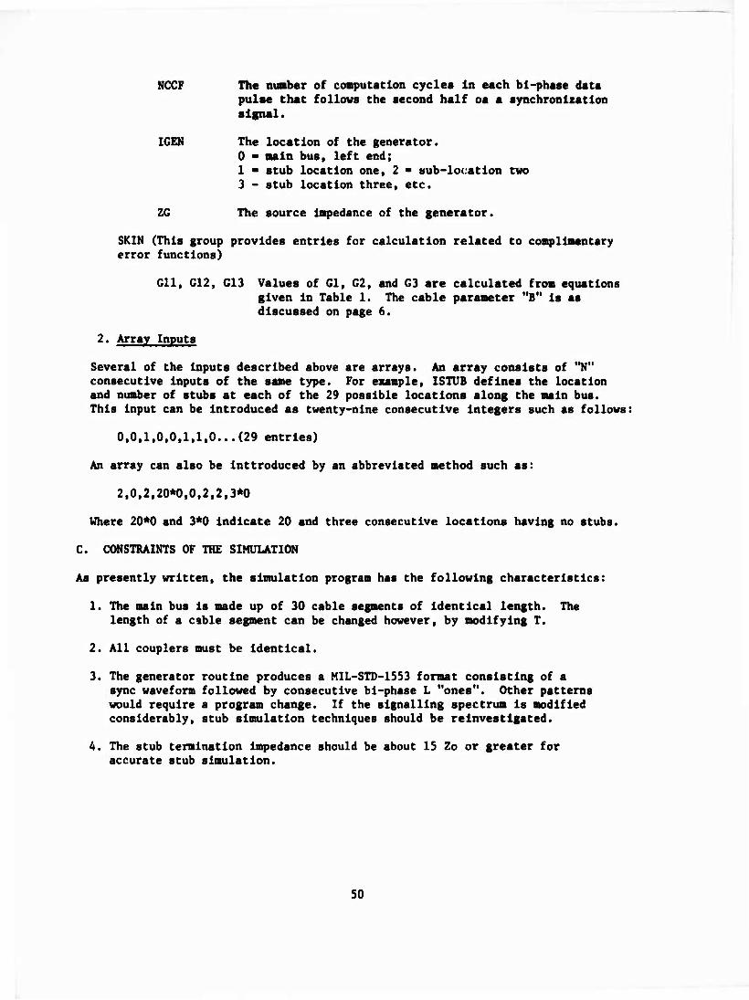
NCCF The number of computation cycles In each bi-phase data pulse that follows the second half oa a synchronization signal.

IGEN The location of the generator. 0 - main bus, left end; 1 • stub location one, 2 - sub-location two 3 - stub location three, etc.

ZG The source Impedance of the generator.

SKIN (This group provides entries for calculation related to complimentary error functions)

Gil, G12, G13 Values of Gl, G2, and G3 are calculated from equations given In Table 1. The cable parameter "B" Is as discussed on page 6.

2. Array Inputs

Several of the Inputs described above are arrays. An array consists of "N" consecutive Inputs of the same type. For example, ISTUB defines the location and number of stubs at each of the 29 possible locations along the main bus. This input can be introduced as twenty-nine consecutive Integers such as follows:

0,0,1,0,0,1,1,0.. .(29 entries)

An array can also be inttroduced by an abbreviated method such as:

2,0,2,20*0,0,2,2,3*0

Where 20*0 and 3*0 indicate 20 and three consecutive locations having no stubs.

C. CONSTRAINTS OF THE SIMULATION

As presently written, the simulation program has the following characteristics:

1. The main bus is made up of 30 cable segments of identical length. The length of a cable segment can be changed however, by modifying T.

2. All couplers must be identical.

3. The generator routine produces a MIL-STD-1553 format consisting of a sync waveform followed by consecutive bi-phase L "ones". Other patterns would require a program change. If the signalling spectrum is modified considerably, stub simulation techniques should be reinvestigated.

4. The stub termination Impedance should be about 15 Zo or greater for accurate stub simulation.

50

5. The length of a stub for display time phasing Is always equal to that of a line element on the main bus. This Introduces a small phasing error when the actual stub length being simulated differs. Effects however, are not easily dlscemable.

6. The length of a stub used to drive the bus from e «tub location Is also always equal to a main bus cable element In length.

7. When multiple stubs are simulated, all stub locations being used must contain the same number of multiple stubs. For example, If 10 stub locations are used and the multiple stub option Is elected, all 10 locations would have the same number of "N" stubs. If N • 4, a total of 40 stubs would load the bus.

D. COUPLER/STUB CALIBRATION DISCUSSION

Coupler/Stub characteristics are determined by the parameter listed under TRANS1 and TRANS2 plus ZL, ZX, REF1 and assigned line length. These parameters describe both dynamic and steady state loading effects.

Dynamic loading parameters consist of WNSQ1, TW0ZW1, R00T2 and the capacltlve load Introduced by the stub length LSTUB array. These parameters are determined by methods dlscustted In Psragraph II-D and/or with aids and references well known to control system design (eg., References 10 and 11).

Steady State loading Is determined by REF1 (I.e., I}), ZL, GAIN1 and GAIN2. REF1 Is calculated from the steady state Input Impedance presented at s stub location In accordance with equation 14.

GAIN1 establishes the voltage levels that appear on the stub end. This para- meter setting Is not generally critical and can be made equal to the no losd steady state output voltage gain of the transformer multiplied by 0.5/|l+Rr.f 1

Reflective calculations at the end of the stub adjust for resistive loading. In the program, the parameter REF4 Is calculated from ZL using equation 14. No specific entry other than ZL is required.

GAIN2 establishes th* steady state voltage fed back onto the bus. This Is an Important Input for accurate simulation with numerous stubs. GAIN2 can be related to the Insertion loss of the coupling network. An equation that can be used to provide this imput Is as follows

CAIH2 - QC - (1 + MfD wuru (1+REF1) (GAiNl)(r4)

where aC - Insertion loss of the coupling (voltage ratio) REF1 • Input parameter GAIN1 - Input parameter

■ reflection coefficient at end of stub determined vis equation 14.

r4

dC Is a measured Insertion loss of the coupler and equal to the voltage on the bus with a loaded coupler divided by the voltage on the bus with no coupler.

51

Multiple stubs are simulated by providing entries that duplicate their loading effects. For example, REF1 is entered as the value of I\ for the number of parallel couplers. The GAIN1 entry is the same as for one stub. The GAIN2 entry can be determined from the equation above with adjusted values of QtC and REF1. Parameters effecting dynamic loading are the same as for a single stub.

52

V. LABORATORY EVALUATION

This section describes the breedboerd hardware used for simulator verifi- cation and provides test data.

A. DATA BUS BREADBOARD

The verification breadboard Is designed In accordance with MIL-STD-1553 design criteria. It consists of coupler units, cable sections of various length, connector mounted resistor terminators and a Bl-phase L breadboard driver. All elements contain compatible connectors so that a variety of data bus configurations are possible without soldering.

Two coupler transformer types (i.e., two different transformers) were purchased by the statement of work. Figure 27 provides a coupler schematic. Transformers and series fault isolation resistors are mounted in small boxes, Pomona model 2397 or 3230.

The transformers were arbitrarily selected to have markedly different parameters. The transformers and key characteristics are as follows:

PE 2244 (Pulse Engineering)

Turns Ratio 1:2

Primary Inductance 6 MHy

Pri/Sec Leakage Inductance 11 UHy*

Winding to Winding Capacitance IS pfd

Primary dc Resistance ^0 ohms

Secondary dc Resistance 24 ohms

PE 2228X (Pulse Engineering)

Turns Ratio 1:1

Primary Inductance 1.3 MHy

Pri/Sec Leakage Inductance 1.5 UHy*

* Measured values.

53

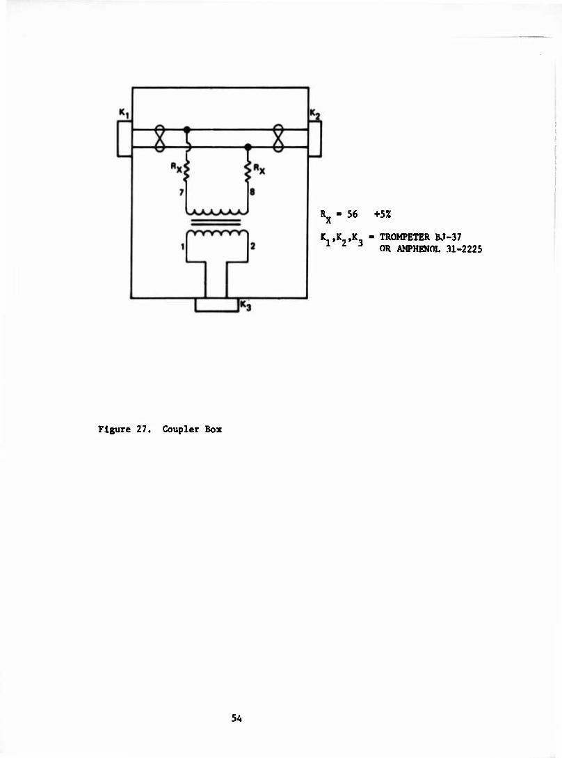
Rx - 56 +5%

K ,K ,K - TROMPETER BJ-37 1 J OR AMPHEMOL .11-2225

Figure 27. Coupler Box

54

Winding to Winding Capacitance 3.6 pfd

Primary dc Resistance 3.6 ohms

Secondsrd dc Resistance 3.8 ohms

Transformer characteristics are as published by the manufacturer except as noted. The 1:2 transformer was connected to provide a step down from the bus to s stub.

The cable sections are fabricated from 68 ohm teflon Insulated twisted shielded pair with 12 twists per foot. Cable Is compatible with MIL-STD-1553 requirements with attenuation characteristics given In Figure 4. Propo- gatlon delay was measured at approximately 1.4 ns/ft. Wire Is ITT type 2A SWTE 1936 AJTM. Cable sections are as follows: eight, 10 feet long; seven, 20 feet long; one, 30 feet long; one, 40 feet long; one, 120 feet long; and two, 2 Inches long.

Termination resistors Include eight 2.2 Kohm resistors for remote terminal load slmulstlon and two 68 ohm resistors for cable end termination.

The Bl-phase L breadboard driver circuit produces three level signalling compatible with MIL-STD-1553. The circuit Is housed In a 6,,x4"x2" chassis with an output chassis connector that mates with the connectors provided on each end of the cable sections. Figure 28 provides a schematic Identifying component parts. Figure 29 shows Input waveform required for operation. The breadboard driver also requires external power supply Inputs of +5 volts, 100 mllllsmps and +8 to +15 volts at 225 mllllamps.

A laboratory pattern generator Is used to operate the driver. DATAPULSE Models 203 and 208 are two examples of compatible pattern generators.

Inputs to the breadboard driver are TTL compatible. Figure 29 defines wave- form Inputs and outputs of the driver.

55

u •H

<J V.

I & ■g

£

X

5«

1 I 8

T i e i

H o > I

5

s o UJ

§5 51 i-

t — i- -

8 X

KS* o >

i o

i- r BC

S7

B. TEST DATA

Basically two test configurations were used for comparing breadboard and siaulator outputs. The first. Setup A (Figure 30), was used for characterizing transformers and stub loading effects of different lengths. The second. Setup B (Figure 31), was used for evaluating eight stub configurations. In Setup B, the generator was moved to different locations which included driving the bus from stub ends as is normally the case in a MIL-STD-1553 application.

Figure 32 shows a unique case of driving 120 feet of cable terminated in 68 ohms. The figure shows photographs taken of waveforms as they appear at both cable ends along with simulator outputs from the identical configuration. Minor distortion noted at the breadboard generator is believed caused by cable characteristic impedance variation with frequency. End termination comparisons agree favorably. The exponential rise effect illustrates skin effect and its simulation.

Figures 33 to 38 reflect data from the coupler that uses 2:1 transformers (PE 2244). Figures 33 «nd 34 show Setup A with different stub lengths and consequently the effects of the capacitance stub loading. Figures 35 and 36 provide comparison ffor eight stub loads of Setup B with generator driving from the left end. Figures 37 and 38 are similar cases except driving from Stub #1, forty feet from the left end of the bus.

Figures 39 and 40 show data comparisons for the 1:1 transformer (PE2228X) coupler units. Figure 39 is a one 20 feet case of Setup A. Figure 40 is the eight stub configuration of Setup B.

Figure 40 indicates that parameter or even a model change would improve simu- lation of data from generator driving from stub to bus.

58

PATTERN GENERATOR

»FT.

POWER SUPPLIES

120 FT. Mi.

STUB (DIFFERENT LENGTHS)

2.2K OHMS C - COUPLER G•GENERATOR

Figure 30. Setup A

<"* <0FT.

0

FT.

10 FT. 10 FT. 10 FT. 10

20 FT

FT.

2.2K 2.2K 2.2K 2.2K

120 FT.

10

20 FT,

FT. 10

20 FT.

FT. 10

WZ>i FT. 10 FT.

-wv- -^/^A>- ^SAA»- -WA^ 2.2K 2.2K 2.2K 2.2K

C- COUPLER G■GENERATOR

Figure 31. Setup B

59

I

fü

I

ta o O m u V J> C 9 •1 w

8 O w u u

S $<< U f^s*

8 V ** t* «J s^w

- ■ i

1 I \ i

o

i-l

i

3

C o CO

I I«

u o

I

IV I- 3 oo

i

5

s

I !

J i ! 3

8 • u

I* S «4 s-§ s <i 5 w

O (O m u »j «J

$* < < 2~. *-S^H

IN

•§ «J ■

s

i o

rf 4

62 IHM!

I o

I

I u o o

o

g u m

I 3 u o

I U1

«

63 I M M «

■

w

u s o

I O

3 u o

i i I i i 6« * ? f 7 T

11« u m u w C m

o ao <M ■ ^ ms

u

C

-o

8 M

O

3 an

i

*i

5

1

i

I 3

i s

I

i

s ! ■a

i

OC ' ■ I . ■ '

S

g u o

!

} 67

■ T

I * T

•

1

w u

x-i O o

•g

HI O W J3

IW IM M » w -H SiH U

M « U O.H < < u —t ^» —~ «I •• f-l (M

C/l H »-'^

i

5 I 5

i. _.i

■

o o

o

68 : T

I ■ ■ • • • 7 T 7

VI. CONCLUSIONS AND RECOMMENDATIONS

The network simulator developed on this program should prove a valuable tool for MIL-STD-1553 application study and for designing couplers. Furthermore, since the program is FORTRAN coded, modifications to the basic software could and should broaden its use.

Because the contract scope was limited, several areas were not investigated as fully as desired. These include the characterization of transformers and stubs. An original goal was to fully simulate transformers from resistance, inductance and capacitance measurements or via similar manufacturer's specifica- tion data. As Indicated in Paragraph II-D, this goal was not achieved. Addi- tional work in this area is recommended. Additional stub analysis is also recommended.

The transmission line algorithm that takes skin effect into account is believed a noteworth development. With three parameters obtainable from laboratory data, an accurate line simulation is achievable for a wide range of transmission lines. Simulation accuracy can be further improved by adding terms and/or by changing calibration points.

69

REFERENCES

1. MIL-STD-1553 (USAF). "Military Standard. Aircraft Internal Time Dlvlalon Multiplex Data Bus," 30 August 1973.

2. W. C. Johnson, "Transmission Lines and Networks," McGraw-Hill Book Company, Inc., 1950, pp. 360.

3. R. E. Matlck. "Transmission Lines for DlRltal and Coosninicatlon Networks,"'McGraw-Hill Book Company, Inc, 1969, pp. 360.

4. R. A. Chlpman, "Transmission Lines," Schaum's Outline Series',' McGraw- Hill Book Company, Inc., 1968, pp. 236.

5. R. L. Ulglngton and N. S. Nahmen, "Transient Analysis of Coaxial Cables Considering Skin Effect," Proceedings of the IRE. February 1957, pp. 166-174.

6. E. F. Boose, "Lessons Learned Through a MIL-STD-1553 Time Division Multiplex Bus," Proceedings of the IEEE 1975 National Aerospace and Electronics Conference (NAECON 1975). June 10-12. 1975. pp. 639.

7. N. R. Grossner, "Transformers and Electronic Circuits," McGraw-Hill Book Company, Inc., 1967, pp. 321.

8. R. Lee,"Electronic Transformers and Circuits," John Wller & Sons, Inc., 1947, 1955, pp. 360.

9. A. Tustin, "A Method of Analyzing the Behavior of Linear Systems in Terms of Time Series," Journal of IEEE. Vol. 94, Part IIA, May 1947, pp. 130-142.

10. C. J. Sovant, Jr., "Control System Design," McGraw-Hill Book Company, Inc., 1958, 1964, pp. 457.

11. J. J. D'Azzo and C. H. Houpis, "Feedback Control System Analysis and Synthesis," McGraw-Hill Book Company, Inc., 1960, 1966, pp. 824.

70