data analysis and correlations for the particulate matter
TRANSCRIPT

University of Tennessee, Knoxville University of Tennessee, Knoxville
TRACE: Tennessee Research and Creative TRACE: Tennessee Research and Creative
Exchange Exchange
Masters Theses Graduate School
5-2001
Data Analysis and Correlations for the Particulate Matter Data Analysis and Correlations for the Particulate Matter
Continuous Emission Monitoring System Test Program at the Continuous Emission Monitoring System Test Program at the
TSCA Incinerator TSCA Incinerator
James A. Calcagno, III University of Tennessee - Knoxville
Follow this and additional works at: https://trace.tennessee.edu/utk_gradthes
Part of the Environmental Engineering Commons
Recommended Citation Recommended Citation Calcagno, III, James A., "Data Analysis and Correlations for the Particulate Matter Continuous Emission Monitoring System Test Program at the TSCA Incinerator. " Master's Thesis, University of Tennessee, 2001. https://trace.tennessee.edu/utk_gradthes/1961
This Thesis is brought to you for free and open access by the Graduate School at TRACE: Tennessee Research and Creative Exchange. It has been accepted for inclusion in Masters Theses by an authorized administrator of TRACE: Tennessee Research and Creative Exchange. For more information, please contact [email protected].

To the Graduate Council:
I am submitting herewith a thesis written by James A. Calcagno, III entitled "Data Analysis and
Correlations for the Particulate Matter Continuous Emission Monitoring System Test Program at
the TSCA Incinerator." I have examined the final electronic copy of this thesis for form and
content and recommend that it be accepted in partial fulfillment of the requirements for the
degree of Master of Science, with a major in Environmental Engineering.
Dr. Wayne T. Davis, Major Professor
We have read this thesis and recommend its acceptance:
Dr. Terry L. Miller, Dr. James L. Smoot
Accepted for the Council:
Carolyn R. Hodges
Vice Provost and Dean of the Graduate School
(Original signatures are on file with official student records.)

To the Graduate Council:
I am submitting herewith a thesis written by James A. Calcagno, III entitled "Data
Analysis and Correlations for the Particulate Matter Continuous Emission Monitoring
System Test Program at the TSCA Incinerator". I have examined the final copy of this
thesis for form and content and recommend that it be accepted in partial fulfillment of the
requirements for the degree of Master of Science, with a major in Environmental
Engineering.
Dr. Wayne T. Davis, Major Professor
We have read this thesis and
recommend its acceptance:
Dr. Terry L. Miller
Dr. James L. Smoot
Accepted for the Council:
Dr. Anne Mayhew
Interim Vice Provost and
Dean of the Graduate School
(Original signatures are on file in the Graduate Student Services Office.)

DATA ANALYSIS AND CORRELATIONS
FOR THE PARTICULATE MATTER
CONTINUOUS EMISIONS
MONITORING SYSTEM
TEST PROGRAM
AT THE TSCA INCINERATOR
A Thesis Presented for the Master of Science Degree
The University of Tennessee, Knoxville
James A. Calcagno, III
May 2001

ii
ACKNOWLEDGEMENTS
I express a sincere gratitude to my major professor, Wayne Davis, for his patience and
steadfast guidance throughout the course of this project. I am also particularly grateful to
the committee members, Terry Miller and James Smoot for their invaluable comments
and kind assistance. A special thanks goes to the Project Manager at the TSCA
Incinerator, Jim Dunn, who provided his time and efforts to make this project a reality.
Another special thanks goes to Marshall Allen at the Hemispheric Center for
Environmental Technology for funding the principal part of this research. Without the
help of this group of people, I would not have been able to bring this project to fruition.
iii
ABSTRACT
A field study was conducted to evaluate the performance of three commercially
available particulate matter (PM) continuous emission monitoring systems (CEMS)
during 1999-2000 at the U.S. Department of Energy (DOE) Toxic Substance Control Act
(TSCA) Incinerator located near Oak Ridge, Tennessee. The incinerator is permitted to
treat mixed-waste, Resource Conservation Recovery Act (RCRA) hazardous and non-
hazardous waste, and wastes containing polychlorinated biphenyls (PCB). The mixed-
waste treated at the incinerator contains both low-level radioactive and hazardous
chemical constituents. The air pollution control system of the incinerator utilizes
Maximum Achievable Control Technology (MACT), which is comprised of a rapid
quench, venturi scrubber, packed bed scrubber, and two ionizing wet scrubbers in series.
The CEMS chosen for the demonstration were two beta-gauge devices and a light-
scattering device. The performance of the CEMS was evaluated using the requirements
in the Environmental Protection Agency (EPA) draft (11-3-98) Performance
Specification 11 (PS11) and draft (11-3-98) Procedure 2. The various possible
combinations of treating liquid, aqueous, and solid wastes simultaneously presented a
challenge in establishing a single, acceptable correlation relationship for the individual
CEMS. The flue gas of the incinerator was also continually at or near saturated moisture
conditions, yet offering an additional challenge to the CEMS. The results of the EPA
reference Method 5i stack tests for establishing the calibration curves demonstrated that
the beta-gauge monitors could meet PS11 criteria, and the light-scattering monitor could
not meet PS11 criteria. Experience seemed to establish however, that more than one set
of correlation tests might be necessary to determine the nature of the calibration curve.

iv
TABLE OF CONTENTS
CHAPTER Page
1 INTRODUCTION ......................................................................................................1
1.1 Research Objective ............................................................................................1
1.2 General Description of PM and CEMS .............................................................3
1.3 Overview of Federal Regulations ......................................................................4
2 LITERATURE REVIEW ...........................................................................................6
2.1 Historical Development .....................................................................................6
2.2 Preliminary Field Demonstrations .....................................................................9
2.3 Technical Approach .........................................................................................10
2.3.1 Reference Method 5i............................................................................11
2.3.2 Procedure 2 ..........................................................................................11
2.3.3 Performance Specification 11 ..............................................................13
2.4 Primary Field Demonstrations .........................................................................14
2.4.1 DuPont Hazardous Waste Incinerator..................................................15
2.4.2 Eli Lilly Hazardous Waste Incinerator ................................................18
2.5 Summary..........................................................................................................20
3 TSCA INCINERATOR AND FACILITY ...............................................................21
3.1 General Description .........................................................................................21
3.2 Incinerator Process System..............................................................................22
3.3 Air Pollution Control System...........................................................................24
3.4 Process Data Collection ...................................................................................27

v
4 CONTINUOUS EMISSION MONITORING SYSTEMS.......................................28
4.1 Durag F-904 K Beta Monitor...........................................................................29
4.2 Environment SA Beta 5M Monitor..................................................................31
4.3 Sigrist CTNR Light-scattering Monitor...........................................................33
5 CALIBRATION TEST METHOLOGY...................................................................36
5.1 Method 5i Stack Sampling Procedure..............................................................36
5.1.1 Sampling Location ...............................................................................36
5.1.2 Sampling Protocol................................................................................37
5.2 Particulate Monitoring Systems.......................................................................38
5.2.1 Installation Locations...........................................................................38
5.2.2 Process Data.........................................................................................39
5.3 Data Collection and Analysis...........................................................................39
5.3.1 Reference Method 5i............................................................................39
5.3.2 CEMS Continuous Raw Data ..............................................................42
5.3.3 Inter-instrument Comparisons .............................................................46
6 RESULTS/DISCUSSION.........................................................................................50
6.1 Quality Assurance Criteria of Procedure 2 ......................................................51
6.1.1 Standardization of the Linear Portion of RSD.....................................52
6.1.2 Slope Criterion .....................................................................................54
6.2 Pre-testing Activity ..........................................................................................54
6.2.1 Phase 1 Correlation Test ......................................................................54
6.2.2 Phase 2 Correlation Test ......................................................................55
6.3 Final-testing Activity (M5i Phase 3 Data) .......................................................58

vi
6.4 PM CEMS (Performance Specification 11).....................................................61
6.4.1 Durag-904 K Beta Monitor..................................................................62
6.4.2 Environment SA Beta 5M Monitor......................................................64
6.4.3 Sigrist CTNR Light-scattering Monitor...............................................67
6.5 Relative Correlation Audit...............................................................................69
6.6 Inter-instrument Comparison Between CEMS ................................................71
7 CONCLUSIONS/SUMMARY.................................................................................74
REFERENCES .........................................................................................................80
APPENDIX ..............................................................................................................84
Appendix A Tables Discussed in Body of Report........................................85
Appendix B Figures Discussed in Body of Report ....................................100
Appendix C Airtech Laboratory Report Phase 3 M5i Testing...................132
Appendix D Summary of M5i and CEMS Data for Phase 3 Testing.........143
Appendix E CEMS Sample Spreadsheet Calculations ..............................145
VITA ............................................................................................................155

vii
LIST OF TABLES
TABLE Page
2.1 Summary of PM CEMS Performance Characteristics (without outliers)
for the DuPont Waste Incinerator ........................................................................86
2.2 Summary of PM CEMS Performance Characteristics (without outliers)
for the Eli Lilly Waste Incinerator .......................................................................86
3.1 Typical Flue Gas Conditions at the Sampling Location Under Normal
Incinerator Operating Conditions ........................................................................87
3.2 Incinerator Process Parameters Monitored During the PM CEMS
Demonstration......................................................................................................88
4.1 Input/Output Signal Requirements for the Purpose of Data Logging..................89
4.2 Summary of PM CEMS Sampling Characteristics..............................................90
5.1 Summary of CEMS Measuring Ranges and Equations for Conversion
Between Milliamp and Concentration .................................................................91
6.1 Estimation of Precision and Rejection of Statistical Outliers for Phase 2
M5i PM Concentration Data................................................................................92
6.2 Summary of Waste Feed Categories, Ash Content, and
Feed Rates for Phase 3.........................................................................................93
6.3 Three Different Levels of PM Concentration Over the Incinerator
Operations for Phase 3 .........................................................................................93

viii
(list of tables continued)
TABLE Page
6.4 Estimation of Precision and Rejection of Statistical Outliers for Phase 3
M5i PM Concentration Data................................................................................94
6.5 CEMS and M5i Phase 3 Data Adapted for Use in the Correlation Tests ............96
6.6 Summary of Durag Phase 3 PS11 Calibration Results ........................................97
6.7 Summary of ESA Phase 3 PS11 Calibration Results...........................................98
6.8 Summary of Sigrist Phase 3 PS11 Calibration Results........................................99
ix
LIST OF FIGURES
FIGURE Page
3.1 Aerial photograph of the TSCA Incinerator demonstration area.......................101
3.2 Overall schematic of the TSCA Incinerator process systems and
the air pollution control equipment....................................................................102
4.1 Front view of Durag F-904 K beta-gauge monitor ............................................103
4.2 General diagram of dilution probe for Durag monitor.......................................104
4.3 Front view of ESA Beta 5M monitor.................................................................105
4.4 Presentation of ESA monitor and probe assemble.............................................106
4.5 Diagram of side view of Sigrist CTNR light-scattering monitor.......................107
4.6 Schematic of Sigrist photometer cell and optical sampling configuration ........108
5.1 Diagram of TSCA Incinerator stack sampling platforms and port elevations...109
5.2 Detail of TSCA Incinerator stack sampling ports..............................................110
5.3 Reference Method 5i sampling train and filter holder assembly .......................111
5.4 Layout of CEMS around incinerator stack ........................................................112
5.5 Schematic representing batch sampling cycle time of beta-gauge monitors .....113
6.1 Phase 2 M5i Cross Correlation (7 Runs Meeting RSD Criteria) .......................114
6.2 Phase 3 M5i Cross Correlation (19 Runs Meeting RSD Criteria) .....................115
6.3 Durag Linear Calibration Curve for Phase 3 .....................................................116
6.4 Durag Logarithmic Calibration Curve for Phase 3 ............................................117
6.5 Durag Polynomial Calibration Curve for Phase 3 .............................................118

x
(list of figures continued)
FIGURE Page
6.6 ESA Linear Calibration Curve for Phase 3........................................................119
6.7 ESA Logarithmic Calibration Curve for Phase 3 ..............................................120
6.8 ESA Polynomial Calibration Curve for Phase 3................................................121
6.9 Sigrist Linear Calibration Curve for Phase 3.....................................................122
6.10 Sigrist Logarithmic Calibration Curve for Phase 3............................................123
6.11 Sigrist Polynomial Calibration Curve for Phase 3.............................................124
6.12 ESA Phase 3 Linear Calibration Curve with Phase 2 Data
Inserted for RCA................................................................................................125
6.13 Sigrist Phase 3 Logarithmic Calibration Curve with Phase 2 Data
Inserted for RCA................................................................................................126
6.14 Durag vs. ESA (1-hour Averages for October 19-22 & 24) ..............................127
6.15 Durag vs. Sigrist (1-hour Averages for October 19-22 & 24) ...........................128
6.16 ESA vs. Sigrist (1-hour Averages for October 19-22 & 24)..............................129
6.17 Durag and ESA Responses vs. Waste Feeds During October 19 ......................130
6.18 Sigrist Response vs. Waste Feeds During October 19.......................................131

xi
NOMENCLATURE
ACA Absolute Correlation Audit
acfm Actual cubic feet per minute
acm Actual cubic meter
AES Airtech Environmental Services
CAA Clean Air Act
CEMS Continuous Emission Monitoring System(s)
CFR Code of Federal Regulations
CI Confidence Interval
cm Cubic meter
CNF Central Neutralization Facility
CO Carbon Monoxide
CO2 Carbon Dioxide
DOE Department of Energy
dscm Dry standard cubic meter
EERC Energy and Environmental Research Corporation
EPA Environmental Protection Agency
ESA Environnement (Environment) SA or Emissions SA
ESC Environmental Systems Corporation
ESP Electrostatic Precipitator
ETTP East Tennessee Technology Park
FRP Fiber-reinforced Polyester

xii
HCl Hydrogen Chloride
HF Hydrogen Fluoride
Hg Mercury
ISO International Standards Organization
IWS Ionizing Wet Scrubber
mA Milliamp
M5i Method 5i
MACT Maximum Achievable Control Technology
mbar Millibar
mg Milligram
min Minute
mm Millimeter
N Normal
N/A Not Applicable
NAAQS National Ambient Air Quality Standards
NaOH Sodium Hydroxide
NG Natural Gas
NESHAPS National Emission Standards for Hazardous Air Pollutants
NSPS New Source Performance Standards
nm Nanometer
O2 Oxygen
P2 Procedure 2
PCB Polychlorinated Biphenyls

xiii
PLA Polystyrene Latex Aerosols
PLC Programmable Logic Controller
PM Particulate Matter
PS11 Performance Specification 11
QA Quality Assurance
QC Quality Control
R or (r) Correlation Coefficient
RCA Response Correlation Audit
RCRA Resource Conservation and Recovery Act
ROM Read Only Memory
RSD Relative Standard Deviation
S ratio Experimental value of deviation (Observed S ratio)
sec Second
SVA Sample Volume Audit
SCDAS Supervisory Control and Data Acquisition System
SO2 Sulfur Dioxide
SSQATP Site-Specific Quality Assurance Test Plan
TI Tolerance Interval
TSCA Toxic Substance Control Act
TÜV (Technischer Überwachungsverein) or Technical Inspection Association.
UD Upscale Drift
WFR Waste Feed Rate
ZD Zero Drift

1
CHAPTER 1
INTRODUCTION
1.1 Research Objective
This thesis summarizes the data analysis and correlation tests that were conducted
to demonstrate and evaluate particulate matter (PM) continuous emission monitoring
systems (CEMS) at the U.S. Department of Energy (DOE) Toxic Substance Control Act
(TSCA) Incinerator located at the East Tennessee Technology Park (K-25) near Oak
Ridge, Tennessee. During July 1999, three PM CEMS were installed on the incinerator:
(1) a Durag F-904K beta monitor, (2) an Emissions SA Beta 5M monitor (ESA), and (3)
a Sigrist CTNR light-scattering monitor. The primary goal of the study was to determine
if PM CEMS operation could satisfy the Environmental Protection Agency (EPA)
requirements in draft Performance Specification 11 (PS11) and the quality assurance
(QA) criteria identified in draft Procedure 2 (P2). Both these guidance documents are
works-in-progress that will eventually appear in CFR 40 Part 60, Appendix B and F,
respectively.
On September 30, 1999, EPA proposed Maximum Achievable Control
Technology (MACT) standards for hazardous waste combustors (i.e., all incinerators,
cement kilns, and lightweight aggregate kilns that burn hazardous wastes). Emission
standards were established in the ruling for several hazardous air pollutants or hazardous
air pollutant surrogates, such as dioxin/furan, mercury, particulate matter, semi-volatile
and low volatile metals, hydrochloric acid/chlorine gas, and hydrocarbons. To verify
compliance with the standards, the EPA also discussed the use of CEMS. Although the

2
final rule did not require the use of CEMS for parameters other than carbon monoxide,
hydrocarbon, oxygen (to provide a dilution correction) and particulate matter, the EPA is
encouraging their use wherever feasible because of certain advantages, which are: (1)
CEMS directly measure the air pollutants; (2) they lead to some degree of certainty
regarding compliance to existing regulations; (3) they allow the public to be better
informed about the emissions from the source at all times; and (4) from a facility
standpoint, CEMS provide real time feedback on combustion processes and allow the
operator to exert a greater degree of control over the operational procedures that might
affect the emissions.
Even though the new MACT standards required the use of PM CEMS, the
installation deadline was deferred because the Agency is still in the process of gathering
additional data to develop source-specific performance requirements. Accordingly, EPA
wished to have more time to resolve other outstanding technical issues that relate to the
implementation of the PM CEMS requirement, such as: (1) the relation of the CEMS
requirement to all other testing, monitoring, notification, and record keeping, (2) the
relation of the CEMS requirement to the PM emission standard, and (3) the technical
issues involving performance, maintenance and calibration of the instrument. Since these
issues will be discussed in later rulemaking decisions, the EPA has deferred the effective
date of the PM-CEMS requirement pending further testing. At present, EPA is also
promoting the use of CEMS for other parameters, such as total mercury, multi-metals,
hydrochloric acid, and chlorine gas.

3
1.2 General Description of PM and CEMS
Particulate matter is a term used to define solid and liquid particles, except
uncombined water, that remain suspended in the atmosphere for extended periods of time
and contain the chemicals or material from the original source. Particulate matter is
known to damage human and animal health, and retard plant growth. Certain pollutant
gases can also form particles through physical and chemical reactions. However, this
type of PM is not the focus of the present study.
The general size range for airborne PM is between 0.001 and 500 µm, though
primary concern is reserved for particles less than or equal to 10 µm because it is in this
range that PM impacts the environment by affecting the transmission of light or visibility.
Smaller particles (less than 0.1 µm) are also easily inhaled and trapped in the alveoli the
lungs, causing various health problems (Wark, Warner, & Davis, 1998). Stationary
sources of fuel combustion, transportation (i.e., mobile sources), and industrial processes
are all major contributors to anthropogenic atmospheric PM. Examples of these sources
of PM are the fossil fuel-burning electric power plants and industrial furnaces, trucks and
automobiles, and the bulk handling of a dry material that can result in the creation of fine
dust.
A continuous emission monitoring system (CEMS), as defined by EPA, is the
total equipment necessary for the determination of a gas, PM concentration, or emission
rate from a stack using pollutant analyzer measurements. Generally a conversion
equation or graph is required to produce the results in units that are applicable to the
emission limit or standard. Continuous monitoring of parameters can determine if a
source is in compliance with the applicable air regulations. The analyzer sends signals to

4
programmable logic controller (PLC). A personal computer utilizing appropriate
software connects with the PLC. Advances in computer technologies also enable the
facility to collect, store, and manage large quantities of data. Collectively, these
components are known as a Data Acquisition System.
1.3 Overview of Federal Regulations
The basic federal standards that regulate or control air pollutants in the United
States are the National Ambient Air Quality Standards (NAAQS), the New Source
Performance Standards (NSPS), and the National Emission Standards for Hazardous Air
Pollutants (NESHAPS). The NAAQS deal with the concentration of pollutants that are
considered permissible in the everyday outdoor atmosphere. Currently there are six
NAAQS pollutants: carbon monoxide, lead, nitrogen dioxide, ozone, PM, and sulfur
dioxide. Ambient-based sampling devices are used to monitor these pollutants.
The NSPS set limits on the amount or concentration of pollutants that may be
emitted from a new stationary source (usually from a stack) into the atmosphere. The
NSPS are further divided into industrial source categories. For example, the NSPS for
new Municipal Waste Combustor established emission standards for cadmium, carbon
monoxide, dioxins/furans, hydrogen chloride, lead, mercury, nitrogen oxides, opacity,
PM, and sulfur dioxide. At this time, the monitoring requirements for certain gaseous
pollutants (e.g., CO, NOx, and SO2) call for the use of CEMS. For the remainder of the
NSPS pollutants (i.e., Cd, dioxins/furans, HCl, Hg, and PM), annual stack sampling is
required using an accepted reference method. Opacity is the notable exception in this
example. A trained and certified observer from ground level, following the provisions
specified in EPA reference Method 9, can determine opacity from visual observations
5
made about the stack plume. Otherwise, the facility can install a monitor that
continuously measures the opacity of the flue gas. Opacity is important because it
provides a relative indication for the concentration of pollutants (e.g., acid gas or PM)
exiting the stack, and as a result, it provides information on the operation and
maintenance of the air pollution control equipment. Nevertheless, opacity is not a true
measure of the mass emission of the pollutants, and furthermore, it has been shown that
instrumental measurements of opacity correlated better with each other than with the
observer measurements of opacity (Conner and White, 1980).
All hazardous air pollutants are essentially regulated under NESHAPS. However
since little progress was actually seen in the reduction of certain air pollutants during the
intervening years after the promulgation of the Clean Air Act (CAA) of 1970,
fundamental modification were made to NESHAPS in the CAA Amendments of 1990,
specifically under Title III. At this stage, each major source (new or existing) is now
required to meet MACT standards, which are defined as not less than the average
emission level achieved by controls on the best performing 12 percent of existing
sources, by category for existing sources, and not less stringent than the emission control
that is achieved in practice by the best controlled similar source for new sources. For
hazardous waste combustors, these standards are being promulgated under joint authority
of the CAA and the Resource Conservation and Recovery Act (RCRA), and as mentioned
previously, the current MACT standards for hazardous waste combustors require the use
of PM CEMS. Thus, there is a need to persist in efforts to develop and demonstrate
instruments that have the ability to accurately measure PM emissions.

6
CHAPTER 2
LITERATURE REVIEW
2.1 Historical Development
There has always been a necessity for better systems to monitor stack emissions
than by conducting manual stack sampling because manual stack tests are time
consuming and do not give daily results about stack emissions. Initially ambient air
analyzers and/or industrial process analyzers were adapted to monitor gaseous pollutants
and/or flue-gas opacity, however these first experimental efforts were not very successful
(Jahnke, 1992). Continuous emission monitoring for PM started in Germany during the
1960s, and the first opacity requirements were promulgated in the United States in 1971.
Throughout the early 1970s, the EPA also funded research to determine if a
transmissometer could be used to estimate PM mass concentration, but the manufacture
of transmissometers for use by in stationary sources did not develop until 1975 with the
establishment of Performance Specification 1.
A transmissometer is an instrument that determines the extinction coefficient and
the visual range or opacity of the atmosphere. It measures the fraction of light from a
collimated light source that reaches a light detector between a fixed distance. A portion
of the light does not reach the detector because it is absorbed or scattered by the medium.
The equation that defines percent opacity is {(1 – T) x 100}. The fraction of light
transmitted, T is (I/Io), where Io is the original intensity of the light at the source, and I is
the intensity of the light at the detector. It has been shown that T = exp(-σd), where σ is
the overall extinction coefficient with units of lenght-1, and d is the path length distance

7
between the light source and the detector. For simplicity, the extinction coefficient used
here included the effects of both light-scattering and adsorption by the gas molecules and
the particulate matter.
Connor and Hodkins (1967) showed that the opacity of smoke from a stack
containing fine particles was affected by the wavelength of light used in the
transmissometer. Their results indicated that the opacity of the plume as measured by a
blue light source was greater than the opacity of the plume as measured by a white light
source (i.e., 40% vs. 25% opacity, respectively). A red light source had less opacity than
the white light source (i.e., 18% vs. 25% opacity, respectively), and the opacity of the
white light source was roughly five-times greater than the opacity of an infrared source
(i.e., 25% vs. 5% opacity, respectively). Connor (1974) also demonstrated that particle
size and light wavelength were functionally related. By means of a white light (average
wavelength about 0.5 µm), the researcher discovered that particles much smaller than the
light wavelength (i.e., particle diameters < 0.05 µm) contributed little to opacity.
Particles much larger than the light wavelength (i.e., particle diameters > 2 µm) were not
a function of the opacity, and for particles about the same size as the wavelength of white
light, opacity showed a strong dependence on particle size.
Conner, Knapp and Nader (1979) correlated opacity and PM mass concentration
measurement separately for three cement (rotary-kiln) plants and three oil-fired power
plants with in-stack transmissometers. Two of the kilns were wet processes systems that
used an ESP for the air pollution control equipment; the other kiln was a dry process
system that used a bag-house for air pollution control. Two oil-fired boilers burned high-
sulfur oil at high excess oxygen conditions, and the other boiler burned low-sulfur oil at

8
low excess oxygen conditions. No air pollution control equipment had been installed on
any of the oil-fired boilers. The researchers discovered that the opacity attenuation
coefficient and PM mass concentration were related, however the slopes of the curves
(attenuation coefficient/mass concentration) were distinctly different at each facility. It
was obvious that a useful correlation existed, but the response from the instrument was
strongly dependent on the operating characteristics that were in effect at the kiln and/or
the boiler.
Philosophies changed within the EPA during the 1980s in relation to particulate
monitoring, and PM CEMS were not a priority again in the U.S. until new initiatives
began in the mid 1990s. The early approach towards PM CEMS in Germany was similar
to the United States. However, the eventual course followed by the Federal
Environmental Agency in Germany lead to wide-range suitability testing and
specifications for particulate continuous monitors. In addition, the European
International Standards Organization (ISO) developed standards for the certification of
PM CEMS that eventually would serve as the guidelines EPA used to draft Procedure 2
(P2) and Performance Specification 11 (PS11) to govern the design, performance, and
installation of PM monitors in the U.S.
Initial tests of transmissometers by the TÜV-Rhineland (the German technical
inspection agency similar to the Underwriters Laboratories in the U.S.) did not produce
results to the satisfaction of the agency. Nevertheless, improvements were made on the
transmissometer, and over 5000 instruments were eventually installed throughout the
country to measure opacity. As emission regulations became more stringent over the
years and air pollution control equipment improved, the PM concentrations decreased to

9
levels that were too low to be accurately measured with simple transmissometers.
Subsequently the emphasis shifted toward optical devices that could measure the forward
or back-scattering of light through a process involving the light beam striking the
particles and detecting certain parts of the scattered light at a some angle between the
light beam and the detector. In this configuration, the concentration of high or low PM is
proportional to the intensity of the scattered light, as long as the particle properties, like
size, shape, color or refractive index do not change appreciably. Consequently, light-
scattering monitors represent about 80 percent of the new PM monitors that were
installed during the 1990s in Germany (Clapsaddle and Trenholm, 2000).
2.2 Preliminary Field Demonstrations
The EPA recognized that the poor correlation between opacity and PM
concentrations near the proposed emission limits was an inherent problem if an opacity
monitor was going to be used to demonstrate compliance since the detection level of
continuous opacity monitors was typically reached at PM concentrations of about 45
mg/dscm @ 7% O2. In 1996 the EPA Office of Solid Waste proposed a rule (Federal
Register; April 19, 1996) that would require the installation and operation of CEMS for
PM and mercury in hazardous waste incinerators. To support the CEMS requirements,
the EPA proposal included draft specifications, test procedures, and quality assurance
requirements for the new monitoring systems. The EPA also had previously solicited
proposal from vendors to participate in the Agency's ongoing field demonstration test
program for PM CEMS (Federal Register; February 27, 1996).
Prior to this initiative, limited field pilot programs were conducted during 1995 at
the Rollins Environmental Services hazardous waste incinerator, located in Bridgeport,

10
New Jersey, and the LaFarge Cement Company hazardous waste kiln, located in
Fredonia, Kansas. Optical (light-scattering) and beta-gauge instruments (i.e. devices that
measure beta radiation attenuation) were tested at both facilities to gain experience in
designing future tests, and to support vendor claims that PM CEMS could be used for
compliance of emission standards. A full calibration of the instruments was also
attempted at the LaFarge plant according to European specifications ISO No. 10155.
From these two preliminary field studies, EPA concluded that the statistical criteria of
ISO 10155 could be used as the basis for Agency's proposed performance specification
for PM CEMS, but the manual gravimetric reference Method 5 (M5) measurements used
in the calibration of the PM CEMS responses exhibited significant variability when
measuring low PM concentrations because of probe washing requirements and the
difficulty in filter recovery (Roberson, 1997).
2.3 Technical Approach
The satisfactory outcome of the preliminary tests mentioned above encouraged
EPA to conduct long-term data gathering field demonstrations of PM CEMS to determine
what accomplishments could be achieved. Yet before discussing the results of the two
most important long-term field studies conducted to date (i.e. by Eli Lilly and Dupont), it
is necessary to review the EPA certification requirements and procedures for PM CEMS.
These documents are either currently still in draft form (i.e. P2 and PS11) or have
recently been included in the CFR 40, Part 60 Appendix (i.e., M5i). Nevertheless, these
documents will eventually serve as the regulatory guidance for all future PM compliance
monitoring for stationary sources located throughout the United States.

11
2.3.1 Reference Method 5i: The EPA determined that much of the variability in
previous attempts to calibrate PM CEMS resulted from inaccuracies in performing the
filter recovery procedure in reference Method 5 (M5). This error would occur when the
PM mass of the total sampling train was very small. Accordingly, the EPA developed a
modified procedure, called M5i and recommend that it be used to calibrate the CEMS
when the PM of the total sampling train is expected to be 50 mg or less. Basically M5i
differs from the traditional M5 through the use of a smaller, lightweight, integrated filter
and filter assembly that can be tared as a single unit. This improves M5 by eliminating
the filter recovery step, and its associated errors due to the loss or contamination of
sample. However, one negative consequence of the smaller filter is that at higher
emission levels, the filter can become plugged. Since it is important that accurate M5i
measurements are obtained for the CEMS calibration, EPA requires that paired sampling
trains be used simultaneously traversing across two 90o axes. If the measurements
between the two samples do not agree, then there is ample evidence that something was
not consistent during the sample collection.
2.3.2 Procedure 2: Since the quality of the calibration curve can be no better that the
quality of the reference method data that is used to develop the curve, it is necessary to
quantify the precision and accuracy of the reference method data based on pre-
determined criteria. Procedure 2 (P2) contains the quality control (QC) and quality
assurance (QA) requirements for the PM CEMS program. It includes a method for
evaluating the M5i data for outliers. The requirements for routine response and absolute
correlation audits, which must be performed on a periodic basis to verify the continued
12
reliability of the initial PM calibration curve are specified in P2, as well as daily
instrument zero and span checks.
When EPA embarked on the CEMS field demonstration test program, they
initially proposed screening the M5 data to remove statistical outliers. At the time, a
statistical outlier was defined as paired-data points with a relative standard deviation
(RSD) greater than 30%, where RDS% = (|Train A – Train B|)*100/(Train A + Train B).
Analyzing the historical M5 data helped EPA develop this criterion, but eventually
several persons, including a vendor with extensive experience with the European
correlation programs, as well as TÜV -Rhineland, recommended that EPA tighten the
RSD criteria (EPA July, 1999). After the Dupont and Eli Lilly field studies, EPA
concurred and promulgated that a graduated precision criterion be utilized to remove M5i
statistical outliers. The criterion was defined as a 10% RSD for PM emissions greater
than or equal to 10 mg/dscm, increased linearly to 25% RSD for concentrations down to
1 mg/dscm with PM concentrations lower than 1 mg/dscm having no RSD limit. Further
discussion clarifying these RSD criteria will be presented in another section of this report.
The critical analytical auditing requirements of Procedure 2 are: (1) the absolute
correlation audit (ACA) which requires an evaluation of the PM CEMS to a series of
reference standards; (2) the response correlation audit (RCA) which involves again
collecting simultaneous CEMS responses and manual reference method data to determine
whether the initial calibration curve of PS11 is still valid; and (3) the sample volume
audit (SVA) which evaluates the accuracy of the PM analyzer to measure the sample gas
volume.

13
2.3.3 Performance Specification 11: The calibration test procedure for PM CEMS is
referred to as Performance Specification 11 (PS11). This procedure differs from the
calibration of gaseous CEMS, which use calibration gases of know concentration to
periodically calibrate the instrument. The PS11 calibration test is carried out by making
simultaneous CEMS and M5i measurements at three different levels of PM mass
concentrations over the full range of operations for the facility. The technique is called
the "correlation". The essential consequence is the development of a statistical
correlation equation between CEMS and M5i results. A minimum of 15 dual-train M5i
runs are required and correlated. At least 20% of the minimum 15 measured data points
should occur in each of the following levels:
• Level 1 (low): from no PM emissions concentration to 50% of the maximum PM
concentration;
• Level 2 (medium): 25% to 75% of the maximum PM concentration; and
• Level 3 (high): 50% to 100% of the maximum PM concentration.
A correlation or regression analysis between M5i measurements and the PM
CEMS responses is then used to develop an equation that will predict the PM
concentration from CEMS response. The calculation method of least squares is applied
to investigate the correlations using three different curve fits: linear, logarithmic, and
quadratic (or a second degree polynomial). The fitness of the curve must meet each of
the following criteria:
• Criterion A: The correlation coefficient "r" shall be greater that or equal to 0.85;

14
• Criterion B: The confidence interval (95%) at the emission limit shall be within
10% of the emission limit value specified in the regulations; and
• Criterion C: The tolerance interval at the emission limit shall have 95%
confidence that 75% of all possible values are within 25% of the emission limit
value specified in the regulations.
The emission limit is defined here as the emission standard reported at the
conditions of the CEMS (e.g., temperature, pressure, and moisture) experienced during
the correlation test. Under PS11 guidelines, extrapolation of the correlation curve is
limited to 125% of the highest measured PM CEMS concentration measured during the
performance testing.
It is significant to note that the PS11 criteria have changed over the course of the
field-testing demonstration programs. The original version of PS11 identified the
correlation coefficient as greater than 0.90, the confidence interval percent within 20%,
and the tolerance interval percent within 35%. Previous PS11 criteria also stated that the
measured data points must lie within 0 to 30%, 30 to 60%, and 60 to 100% of the
maximum PM concentration for the three levels, respectively that are listed above
(Federal Register; December 30, 1997). The confidence interval (CI), and tolerance
interval (TI) now proposed are at the same level as specified in the European ISO Method
101055.
2.4 Primary Field Demonstrations
Based on surveys done in Europe and preliminary testing done in the U.S., the
EPA has determined that CEMS exist that can quantitatively measure PM mass

15
concentrations, rather than opacity. The two types of analytical instruments that currently
dominate the market employ either light-scattering technology as the detection principle
or carbon-14 beta attenuation technology. As previously stated, EPA's major field
demonstration programs for PM CEMS began in 1996. The program included two
phases: calibration testing to compare and evaluate results from each of the CEMS with
the manual reference method and endurance testing over six months to critically examine
CEMS performance relative to stability of the calibration and the reliability of continuous
operation. The EPA also believed that hazardous waste incinerators represented the
worst-case challenge to PM CEMS because they burn a wide variety of wastes to produce
PM with a sufficient variation in characteristics (i.e., composition, size distribution,
shape, and index of refraction). Many hazardous waste incinerators, in addition, utilize
wet scrubber systems to control emissions, which result in flue gas with a saturated
moisture content, yet another challenge for the CEMS. Lastly, hazardous waste
incinerators have highly efficient air pollution control equipment, which requires CEMS
testing at very low emission levels (Roberson, 1997).
2.4.1 DuPont Hazardous Waste Incinerator: The DuPont facility is located in
Wilmington, Delaware. The incinerator can burn solid and liquid wastes. The air
pollution control system was equipped with spray dryer, cyclone, reverse jet gas
cooler/condenser, a variable-throat venturi scrubber, neutralizing spray absorber,
chevron-type mist eliminator, electro-dynamic venturi, and centrifugal droplet separator
(in that order). The flue gas is then passed through an induced draft fan and a series of
steam heat coils before finally being exhausted from the stack. Preliminary
measurements showed that PM emissions ranged between 10 to 100 mg/dscm at 7% O2.

16
The estimated particle size distribution was approximately 90% < 1 µm. The average
temperature and moisture conditions in the stack were about 320 oF and 25% moisture by
volume.
For this field demonstration, six CEMS were tested representing three different
measuring technologies: optical, beta-attenuation, and acoustic energy. Three of the
CEMS were light-scattering monitors: Durag model DR-300-40, Environmental Systems
Corp. (ESC) model P5A, and Sigrist model KTNR. Two of the CEMS were beta-gauge
monitors: Verewa model F-904-KD and Emissions SA (ESA) model Beta 5M. The final
monitor was a Jonas Inc. model Acoustic Energy PM. Both beta monitors and the Sigrist
monitor employed an extractive, heated, and close-to-isokinetic probe sampling system
that conveyed the sample to measuring sensors external from the stack. The remaining
two optical systems and the acoustic monitor used an insitu sampling and measurement
approach. The acoustic monitor did not produce acceptable results throughout the field-
testing period and was not discussed further in the Dupont report.
Reference Method 5 (M5) calibration tests were performed over a 9-month period
from September 1996 to April 1997. Response Correlation Audits (RCA) were also
conducted during May 1997 to meet the requirements of Procedure 2. During the
calibration tests, six different groups of fuel/wastes were fed into the combustion
chamber: (1) fuel oil, (2) solids including shredded paper, animal bedding, and
office/laboratory waste, (3) high-chlorinated solvents, (4) a mixture of low and/or non-
chlorinated,(5) paint pigments containing water, resins, and solvents, and (6) jugs
containing non-, low- or high-chlorinated solvents. The M5 data were compared to the
output of the five CEMS according to draft PS11 criteria.

17
The tests from December 1996 through March 1997 established the initial
calibration relationship. The total database contained 43-paired M5 and CEMS
responses. Seven of the paired M5 runs were rejected because they were statistical
outliers. A second round of calibration tests was conducted in April 1997. A total of 17-
paired M5 runs and CEMS responses comprised this database, but two paired M5 runs
were outliers and rejected from the database. The investigators decided that the
September through November 1996 tests should only be used as a trial-and-error learning
experience and not incorporated into the final cumulative database, but these results are
included here to demonstrate the difficulty of obtaining valid PS11 calibrations before the
operators have become thoroughly familiar with CEMS response and have fully
characterized the PM emissions across the full range of incinerator operating conditions.
The PS11 acceptance criteria data are shown in Table 2.1 only for the linear
regression analysis that was conducted at the 34 mg/dscm @7% O2 emission limit. (All
tables and figures can be found/are located in the appendix). Based on this data and other
information, the following conclusions were reached:
• None of the CEMS met any of the PS11 criteria during the September to
November 1996 (pre-testing) period.
• For the first data set, each of the five CEMS, with one exception produced data
meeting the PS11 criteria. The Sigrist did not achieve the tolerance interval
measure at 25% for linear regression at the emission standard.
• For the second data set, all of five CEMS met the PS11 criteria. Then again, the
Sigrist monitor was very close to not passing the tolerance interval criterion (i.e.
24.9% vs. 25%).

18
• When the slopes of the linear curves were compared between the first and second
calibrations, the percent difference was within 4% for the beta monitors and
within 7% for the Durag light-scattering monitor. However, the percent
difference was 11% for the ESC and 22% for the Sigrist, both light-scattering
monitors.
• The large percent difference between the first and second calibration curves for
the ESC and Sigrist tended to imply that the linear regression equation was not a
suitable fit for these monitors. When a logarithmic regression equation was used
for the two monitors, agreement between the first and second calibration curve
was within 2%. Although the logarithmic regression fit the data, only the ESC
monitor passed PS11 criteria for both the first and second calibration data sets.
The Sigrist yet again failed to pass the tolerance limit criteria on both the first and
second calibration data.
• Except for the Verewa during the initial calibration period, each monitor produced
data during the RCA tests (i.e., at least 75% falling within ± 25% of the proposed
emission limits). However, the RCA tests were not performed in strict
accordance with P2.
2.4.2 Eli Lilly Hazardous Waste Incinerator: The Eli Lilly facility is located in Clinton,
Indiana. The incinerator only burns liquid and aqueous wastes. The air pollution control
system is equipped with a quench chamber, venturi scrubber, a demister tank, and
scrubber tower in that order. Average temperature and moisture conditions in the stack
were approximately 170 oF and 35% moisture by volume. The field demonstration
program extended over an 11-month period. Two sets of calibration tests were

19
conducted. Phase I occurred from February 1998 to May 1998, and Phase II occurred
from November 1998 to December 1998. Two CEMS were tested during both phases of
the field demonstration: Sigrist model KTNR/SIGAR 4000 light-scattering monitor and
Environmental SA (ESA) model Beta 5M beta-gauge monitor. Both monitors employed
an extractive, heated probe system to deliver a sample to measuring sensors external from
the stack. However, only the ESA monitor adjusted the gas-sampling rate to maintain
isokinetic flow conditions at the probe nozzle. The same monitors were used during the
second phase of the demonstration, but the ESA monitor had been mechanically modified
to allow it to operate at higher moisture levels, and the Sigrist monitor was prevented
from auto-ranging during the calibration test. A second beta-gauge monitor, a Durag
model F-904, was added during Phase II, as a learning experience for the vendor, but the
results were not reported in the final Eli Lilly report.
Various combinations of natural gas and waste types were burned in the
incinerator during the M5i calibration test. Organic waste was always fed into the
primary burner. Aqueous waste, a high salt concentrations waste, and waste spiked with
tin chloride were fed into to the secondary injection ports. The water injected into the
wet scrubbing system was also manipulated to control stack temperatures and thus
produce different levels of moisture in the flue gas during the testing. During Phase I, a
total of 74 paired M5i tests were completed. Five M5i paired tests did not meet the
sampling criteria and were discarded from the Phase I data set. The particulate levels
ranged from 17 to 45 mg/dscm @ 7% O2. During Phase II, a total of 40 M5i tests were
conducted, and five M5i paired tests were also discarded from data set. The particulate
levels for Phase II ranged from 1 to 64 mg/dscm @ 7% O2. The acceptance criteria data

20
are shown in Table 2.2 for the PM CEMS for the Phase I and Phase II calibration tests.
The following conclusions were reached:
• Neither monitor met the draft PS11 criteria in the Phase I test for the correlation
coefficient, but both monitors passed all the PS11 acceptance criteria during the
Phase II test.
• Evaluation of the Phase II data showed that the best correlation relation was
logarithmic for the Sigrist monitor and linear for the ESA monitor.
• No RCA tests were conducted to determine the long-term stability of the
calibration curves thus established in Phase II.
2.5 Summary
The use of continuous PM monitors is feasible for regulatory compliance, however there
are many factors that could significantly influence the ability to calibrate the monitor and
for it to maintain a calibration relationship. While relatively uncomplicated, actual
sample extraction and measurement have proven much more difficult in practice than in
concept. Reliable operations of CEMS over prolonged periods of time have also not been
sufficiently demonstrated. It has been hypothesized that changing the waste streams and
the stack conditions in the incinerator will produce PM with different characteristics, and
as a result, influence the reliability of the calibration curve developed with an optical
CEMS. The EPA still feels that more time is needed to resolve the outstanding technical
issues concerning PM CEMS. Since the technologies may not be adequate at this time,
the EPA has not yet required implementation of the PM CEMS requirement for
hazardous waste incinerators as of April 2001.

21
CHAPTER 3
TSCA INCINERATOR AND FACILITY
3.1 General Description
Wide ranges of waste categories are treated at the TSCA incinerator. These
categories include oils, solvents and chemicals, aqueous liquids, solids, and liquid-free
sludges. The TSCA facility holds federal and state permits to thermally treat mixed-
waste, RCRA hazardous and non-hazardous wastes, and wastes containing
polychlorinated biphenyls (PCB). Mixed-waste is a waste that contain both radioactive
and hazardous chemical constituent. In the recent MACT ruling for hazardous waste
incinerators, the EPA has decided that those standards were also compatible with the
controls for mixed-waste incinerators.
The TSCA incinerator is a rotary-kiln furnace with a secondary combustion
chamber. A wet scrubber air pollution control system is used for cleaning the effluent
gases to comply with TSCA and RCRA regulations, as well as with the air emission
standards for the state of Tennessee. The facility includes various support buildings for
operator and maintenance personnel, the unloading and storage of waste in above ground
tanks, an incinerator area, and concrete wastewater collection/holding ponds. An aerial
photograph of the facility taken during 1995 is shown in Figure 3.1. (All tables and
figures can be found/are located in the appendix).
The high heat-of-combustion liquids are burned in the rotary kiln (the primary
combustion chamber) and in the secondary combustion chamber with dual-fuel (natural
gas/liquid waste) burners. However, aqueous wastes (i.e., liquid wastes containing at

22
least 60% water content) are injected through a lance only into the primary combustion
chamber. Solid and sludge materials are received and stored in metal containers but are
repackaged into combustible cardboard containers prior to incineration. The
containerized solids and sludges are inserted into the rotary kiln by a hydraulic ram. The
hazardous waste incinerator permit conditions allow for both solid and liquids to enter the
rotary kiln, however only liquids may enter the secondary combustion chamber.
The off-gas from the secondary combustion chamber is passed through a multi-
stage air pollution control system for cooling, removal/neutralization of acidic by-
products, and removal of particulate matter (PM). The air pollution control system
includes a quench chamber, a low-energy venturi scrubber, a packed bed scrubber, and
two Ceilcote ionizing wet scrubbers (IWS®). Preceding the stack, an induced-draft fan is
located downstream of the air pollution control system. The effluents from the wet
scrubbers are pumped into holding ponds to allow settling of suspended solids. After a
certain period of time and without disturbing the bottom sediment, the accumulated
wastewaters in the holding ponds are transferred to the ETTP existing Central
Neutralization Facility for final treatment. Solid-type wastes, such as scrubber sludge,
residues from the incinerator wet ash removal system, and the sediment in the holding
ponds are collected in steel drums for subsequent offsite disposal at a commercial landfill
(EERC, 1999).
3.2 Incineration Process System
Auxiliary natural gas is used to maintain the minimum incineration temperatures
inside the primary and secondary combustion chambers to ensure the stable destruction of
wastes. A schematic of the incinerator process system is shown in Figure 3.2. To

23
atomize the primary liquid waste, steam is fed through the burners with the liquid waste.
The steam flow rate is controlled at a constant fixed ratio with respect to the waste flow
rate. The normal operating temperature inside the kiln is maintained at approximately
1800 oF. The rotary kiln also receives and incinerates the boxes of solid and sludge
wastes, which are fed by a hydraulic ram. A burner nozzle injects liquid wastes, and a
lance injects aqueous wastes; both nozzle and lance are located at the kiln faceplate. The
outer shell of the kiln is made of carbon steel; the inner shell is lined with refractory
brick.
The next stage of the incineration process is the mixing chamber. It separates the
primary combustion chamber (rotary kiln) and the secondary combustion chamber. The
mixing chamber collects the hot gases and ash discharged from the rotary kiln. It is also
constructed of carbon steel and is lined with refractory brick. The cross-sectional area of
the mixing chamber is larger than the cross-sectional area of the rotary kiln, so the gas
velocity is reduced, allowing larger PM to fall to the bottom of the chamber. The ash
handling system conveys the residue from a water-filled trough beneath the mixing
chamber to the ash hopper for disposal. Water in the ash trough provides a seal against
air leakage. A circulation pump removes the suspended ash and solids from the water
trough at the bottom of the mixing chamber and conveys the material to the purge water
sumps.
The secondary combustion system receives the hot gases from the mixing
chamber. The cross-sectional area at the entrance to the secondary combustion chamber
is smaller so as to rapidly increase the gas velocity, providing turbulence and mixing of
the kiln gas. Auxiliary natural gas and secondary liquid wastes are fired in the burners.

24
The secondary combustion chamber can receive liquid wastes pumped from the primary
waste feed tanks or the fuel oil tanks, though it usually accepts secondary organic liquid
wastes pumped from secondary waste feed tanks. The normal operating temperature in
the secondary combustion chamber is maintained above 2200 oF. The off-gases from the
secondary combustion chamber pass through a duct to the air pollution control system.
All sections of the secondary combustion chamber are constructed of carbon steel and are
refractory lined.
An induced-draft fan is provided within the system to draw gases from the kiln
through the process equipment line and to discharge gases through the stack into the
atmosphere. In the event of an induced-draft fan shutdown or an interruption of the water
flowing to the quench chamber in the wet scrubber systems, a thermal relief vent at the
outlet of the secondary combustion chamber can release combustion gases to the
atmosphere. This prevents damage to the scrubber during an interruption of quenching
and prevents backward flow from the incinerator during a shutdown of the induced-draft
fan. When the thermal relief vent is activated, all waste material and fuel feeds to the
incinerator are automatically discontinued except for natural gas to the secondary burner
(EERC, 1999).
3.3 Air Pollution Control System
The air pollution control system is a wet scrubber process that reduces both acid
gases and PM from being released into the atmosphere. A schematic of the air pollution
control equipment is shown in Figure 3.2. The hot flue gas received from the secondary
combustion chamber is first cooled in a quench chamber. The system is supplied with
fresh water and is equipped with a recycle water system and an emergency water backup

25
system. The quench chamber normally receives the hot flue gas at about 2200 oF
(containing PM, SO2, HF, and HCl) and saturates the flue gas to the adiabatic saturation
temperature with a series of internal sprays of fresh and re-circulated water. The spray
nozzle system has strainers installed on the supply lines to prevent clogging. The excess
water from the fresh water spray header flows by gravity to the quench chamber recycle
tanks, and pumps re-circulate this water back to the quench chamber. The pH of the
recycled water is controlled with a 20% NaOH solution from the caustic storage tank.
The quench chamber has an acid-resistant refractory lining, which is suitable to withstand
the flue gas temperature and corrosive nature of the scrubbing water. The saturated gas
stream from the quench chamber flows through a fire-retardant fiber-reinforced polyester
(FRP) duct to the inlet of the venturi scrubber. With the exception of the venturi damper
and the induced-draft fan, all of the air pollution control devices downstream of the
quench chamber are manufactured of FRP materials.
The venturi scrubber receives the cooled water-saturated flue gas, removes some
PM greater than 1-micron, and neutralizes a portion of the acid gases (HCl and HF). The
venturi scrubber consists of converging and diverging cones with an automatic variable
throat to maintain a pressure differential and an integral water collection sump. The re-
circulating water system from the quench chamber supplies the scrubber solution
upstream of the venturi throat through a nozzle, and the recycled water flows back to the
quench sump. Again, the pH of the recycled water is controlled using a 20% caustic
solution. A mist eliminator between the venturi scrubber and the packed-bed scrubber
removes the entrained water from the saturated flue gas and minimizes the interference
between the cross-flow liquid/gas flow in the packed-bed scrubber. In addition preceding
26
the mist eliminator, a dispersion plate distributes the gas flow more evenly before it
reaches the mist eliminator. From the mist eliminator, the liquid effluents flow by gravity
back into the quench chamber sump.
The packed-bed scrubber is a horizontal cross-flow unit that contains three feet of
irrigated packing and has an entrainment separator following the packed bed. The
scrubber functions to remove soluble and reactive gasses, such as HCl, HF, and SO2. Re-
circulated scrubber water irrigates the packing, however the water recycle system that
serves the IWS units provides recycled water for the pack-bed scrubber. The pH of the
recycled water is controlled with 20% caustic solution from the caustic solution storage
tank. The packed-bed scrubber has an integral sump, and water flows from this sump
towards the IWS sumps. The process gas from the packed-bed scrubber flows through an
inlet transition duct to the IWS. This provides gradual changeover from the packed-bed
to minimize turbulence before the gas enters the IWS.
Two identical IWS units are located in series. They remove PM of less than 1-
micron from the flue gas stream with high efficiency. The key features of the IWS units
are (l) an ionizing module for electrically charging particles, (2) a packed-bed section for
removing charged particles, (3) a re-circulating water system, and (4) an integral sump.
Both IWS units operate on a continuous basis, with the exception of the following:
alternating every four hours, each IWS unit goes into a water flush cycle to remove the
buildup of PM on the plates, Tellerettes, and other surfaces. During the flush cycle, the
IWS operating voltage drops to zero, and the plates, etc. are flushed with recycled IWS
scrubber water for about five minutes. The gas subsequently passes through a flow

27
control damper section, which is used to vary the stack gas velocity at the outlet of the
IWS to the induced-draft fan.
The induced-draft fan maintains negative pressure throughout the incinerator
system and discharges the water-saturated flue gas to the stack. The fan is constructed of
Hastelloy. Instrumentation and controls measure gas pressure, temperature, fan drive
motor power, and vibration. Loss of the fan operation shuts down all waste feed streams
and the auxiliary fuel to the rotary kiln. A short FRP duct section carries the gas stream
from the fan outlet to the stack inlet and then vents the gas stream to the atmosphere. The
stack is constructed of FPP materials and is 100-feet high with a 54-inch inside diameter.
The current amps and pressure drop across the induced-draft fan are used to provide an
approximation for combustion gas velocity. The stack is equipped with several ports for
sampling flue gas and continuous sampling systems for CO, O2, and CO2, and
radionuclides. The typical flue gas conditions found inside the stack at the sampling
locations under normal incinerator operations are shown in Table 3.1 (EERC, 1999).
3.4 Process Data Collection
The entire combustion process and off-gas cleaning systems are monitored with
process computers. Operational parameters are automatically recorded every 15-seconds
by the incinerator Supervisory Control and Data Acquisition System (SCADA). The
facility has conventional flue gas monitoring systems for O2, CO, CO2, stack gas
temperature, stack pressure, and gas flow rate. Table 3.2 lists key process data that are
collected during the demonstration in order to interpret incinerator operations and convert
the manual test data into the same units reported by the CEMS (EERC, 1999).

28
CHAPTER 4
CONTINUOUS EMISSION MONITORING SYSTEMS
Three PM CEMS were evaluated during this field demonstration: (1) a Durag F-
904 K Beta Monitor, (2) an Emission SA Beta 5M Monitor, and (3) a Sigrist CTNR
Light-scattering Monitor. All three instruments extract flue gas through heated sampling
lines. The Durag and Sigrist monitors are programmable to deliver a slightly greater than
isokinetic sample to the analyzer. Only the ESA monitor is designed to maintain true-
isokinetic sampling conditions at the probe nozzle. However, isokinetic sampling is
generally not critical for small particles less than about 3 µm in diameter because small
mass minimizes the inertial effects of particles entering the nozzle (Lodge, 1988).
The Durag and ESA instruments are batch-sampling devices that collect PM on
filter tape. The measurement principle is based on the absorption of beta radiation, which
is emitted from a radioactive source (carbon-14) located in the sampling apparatus. Both
beta-gauge monitors in their present configuration produce a signal on the order of every
10 to 15 minutes. The significant appeal of beta-gauge technology is that the
instrument’s response is independent of the PM characteristics, such as refractive index,
particle size and density. The Sigrist monitor, on the other hand, is a true-continuous
extractive sampler, and it employs light-scattering as the measurement principle. The
primary advantages of this technology are (1) the response is almost instantaneous, and
(2) because there are fewer moving parts, the instrument is very reliable. The primary
drawback of the light-scattering technology is that the response from the instrument is
very dependent on the PM characteristics, for example composition, density, particle size

29
distribution, and index of refraction. The CEMS are described in further detail in the
following sections. The signal input/output requirements for the CEMS with the data
logger (i.e., the SCADA system) are listed in Table 4.1.
4.1 Durag F-904 K Beta Monitor
The Durag (formerly manufactured by Verewa) F-904-K beta PM monitor
extracts a heated sample from the stack at slightly greater than isokinetic conditions. A
programmable sampling flow rate is maintained with a vacuum pump, as isokinetic
sampling is not actively controlled in response to changes in the gas velocity and
temperature inside the stack. The sample gas is diluted with filtered recycled dry gas
because the flue gas is in a wet saturated condition. The dilution gas is mixed with the
extracted flue gas in the cyclonic mixing chamber of the nozzle. The total sample passes
through heated sections consisting of the probe, sample line, and filter housing. The PM
in the sample is then collected on filter tape. After passing through the filter tape, the
sample gas is dried in a chiller, and the flow rate is measured. A portion of this clean
dried sample gas is recycled and used for the dilution air. Figure 4.1 shows a frontal
view of the Durag monitor, and Figure 4.2 shows the sampling probe and mixing nozzle.
The Durag monitor is commonly referred to as a continuous batch sampler. The
filter tape mechanism has an emitter-detector location for analysis and a sampling
location for gas extraction. In the direction of the tape movement, the sampling
mechanism precedes the emitter-detector mechanism. The carbon-14 source emits beta
radiation (electrons), and a Geiger-Muller counter is used to detect the pulse rate of these
electrons as they penetrate the filter and PM collected on the filter. The PM measurement
cycle first begins by analyzing a clean area (spot) on the filter tape for a fixed period of

30
time. This is called the zero-test; a clean filter area is transported into position (i.e., into
the emitter-detector location), and the spot is exposed to the carbon-14 source, and beta
attenuation is measured through the tape. The drive roll mechanism next positions this
same section of filter tape into the sampling location, the vacuum pump is activated, and
a gas sample is drawn through the filter tape. The filter tape is then transported to the
measurement position (i.e., again to the emitter-detector location) and the filter spot is
evaluated by exposure to the carbon-14 source, and the Geiger-Muller counter measures
the pulse rate of beta radiation through the spot. Thus, the pulse rate through the same
filter spot is measured before and after sampling. The difference between these two
measurements is directly proportional to the PM mass collected on the filter tape.
A microprocessor calculates the PM concentration, given the mass collected and
dry sample volume, and reports the concentrations on a dry standard basis via a 4-20
milliamp signal or in units (mg/Nm3). The monitor is preprogrammed to report PM at
European Normal (N) conditions, which are temperature at 0 oC and pressure at 1013
mbar. In addition, the Durag monitor allows for the conversion of the signal to several
reporting conditions. For this field test demonstration, the monitor was programmed to
report concentration at the U.S. standard conditions, which are temperature at 20 oC and
pressure at 1013 mbar, via the 4-20 milliamp signal or in units (mg/dscm). Note that the
concentration is not reported on a normalized oxygen basis (i.e., the units dscm contain
the actual oxygen condition existing in the stack).
The gas sampling and analysis times can be programmed; therefore different
reporting times can be obtained depending on the PM loading and filter cake porosity. A
typical sample analysis requires two minutes to perform for both the blank (zero-test) and

31
the analysis of the dust loaded filter spot with about one minute of total time for the back
and forward motions of the tape. For example, if the actual sampling time were set at
five minutes, then a complete measuring cycle would occur approximately every ten
minutes. The same spot on the filter tape can be used multiple times, however for the
present demonstration, a clean section of filter tape was used during each measurement
cycle.
The probe and sampling line can be purged with clean dry air to remove deposited
PM. The initiation of the purge cycle is also programmable and is usually set at one
purge per hour. The instrument does automatic zero drift (ZD) and upscale drift (UD)
checks to meet quality control (QC) requirements and features several status signals for
identifying operational modes error flags. The operational modes for calibration are
“zero-signal” and “reference-signal”. The error flags are filter plug indication (vacuum-
error), emissions higher than set point (measuring range-error), total volume higher than
set point (volume-error), and broken filter tape (filter-tear). A summary of the important
system parameters that were in effect during this field study is shown in Table 4.2.
4.2 Environment SA Beta 5M Monitor
The Environment SA Beta 5M (ESA) extracts flue gas through a heated probe. A
pitot-tube and thermocouple are used to determine the stack velocity and the required
isokinetic sampling rate. A microprocessor tests for changes in gas velocity and
temperature in the stack and automatically maintains isokinetic conditions at the probe
nozzle by controlling compressed air through a pneumatic ejector to create a vacuum for
sample collection. The sample gas passes through heated sections consisting of the
probe, sample line, and filter holder housing. The dust sample is collected on filter tape.

32
The ESA monitor is also a continuous batch sampler like the Durag monitor. The
filter tape mechanism has an emitter-detector location and a sampling location. In the
direction of the tape movement, the emitter-detector mechanisms precede the sampling
mechanism. This arrangement of analysis and sampling location was in reverse order for
the Durag monitor, however the essential mechanics of tape movement are basically the
same for both beta gauge monitors. The filter tape mechanism first positions a portion of
clean filter tape in the emitter-detector location and a Geiger-Muller counter measures the
pulse rate of beta radiation from a carbon-14 source through the section of filter tape.
The mechanism then positions the filter area into the sampling location, and flue gas is
drawn through the filter section. Finally the tape mechanism returns the filtered section
back to the emitter-detector location, and the Geiger-Muller counter measures the pulse
rate of beta radiation through the sampled filter spot. Likewise using the differential
method (i.e., taking into account the clean and dirty filter), the final analysis is directly
proportional to the PM mass that was collect during the sampling period.
The sampling duration is programmable and is measured along with the sample
flow-rate. Sampling time is usually set at five to 10 minutes for typical applications. It
can be set lower for higher PM concentration and filter cake porosity. The pre and post
analyses (i.e., measurements of clean and dirty filter) each take about two minutes, and
the total time during filter indexing is about one minute. Thus, a complete measurement
cycle is made every ten to fifteen minutes. A microprocessor calculates the PM
concentration, given the measured mass collected and the volume of gas sampled. The
PM concentration data are reported on an actual basis either as a 4-20 milliamp signal or
in units (mg/Nm3). In this situation, actual conditions are only for the actual conditions

33
of oxygen and moisture in the stack. The ESA response is also internally corrected to the
European Normal (N) conditions, which are temperature corrected to 0 oC and pressure
corrected to 1013 mbar. At the end of each sampling period, the probe nozzle is
momentarily closed, opened, and closed again under vacuum, in order to re-entrain any
PM that may have been deposited in the probe and sampling line.
The instrument produces two status signals (flags) called “stand-by” and “general-
alarm”. The former is for identifying suspect data or encountered problems during
normal operation; the latter is for identifying operational modes for maintenance or
calibration. The instrument makes continuous checks of its main components and signals
any fault with a plain language message (e.g., paper tear fault), however the monitor must
be assessed through the keyboard to display these plain language fault messages. The
ESA unit features data sensors to report sample intake volume, stack gas temperature and
velocity, and venturi tube temperature and static pressure. Figures 4.3 and 4.4 are
diagrams of the ESA monitor and probe assembly. Table 4.2 contains a summary of the
important system parameters that were in effect during the field study.
4.3 Sigrist CTNR Light-scattering Monitor
The Sigrist model CTNR is a light-scattering monitor. Figure 4.5 is a diagram of
the major components of the monitor. Using a fan (blower) to create a vacuum, the
instrument extracts a heated gas sample from the stack at a constant flow rate. A smaller
portion of this sample is passed through a light photometer cell. The entire gas sample is
then returned to the stack. A purge system using pre-filtered air keeps the walls and
windows of the photometer flow cell from being fouled by the extracted sample as it
passes through the flow cell. Figure 4.6a is a schematic of the photometer. The Sigrist

34
monitor is programmed for the probe to sample at slightly greater than isokinetic
conditions to reduce the relative error for changing gas flow velocities in the stack.
The illuminant light source is an incandescent bulb emitting between 360 and
2,800 nm. Figure 4.6b is a schematic of the optical sampling configuration. The
photometer measures only a certain part of the forward scattered light under a 15o angle.
The design incorporates the alternating-light dual beam method. The light is divided into
two beams by a semitransparent mirror. One beam enters the sample where the dust
particles scatter light in all directions. The 15o angle scattered light serves as the
measurement signal. The second beam passes through a stable reference standard and
serves as the reference signal. A chopper disk allows the measuring beam and reference
beam to alternate through the photo-detector. The chopper disk also has a third position
in which both beams are blocked. This serves as the zero value. Thus, the photo-detector
receives three signals one after the other: (1) the measurement light with zero value (2)
the reference light with zero value, and (3) the zero value alone. The zero value is
subtracted from the two signal beams. The final value (i.e., the scattered light intensity)
is established as the ratio of the measured beam to the reference beam. The intensity of
the scattered light is linearly related to the concentration of the particles, as long as the
properties of the particles (e.g., size, shape, color, or refractive index) do not change
appreciably. This design along with the internal electronics is inherently self-
compensating in its PM measurement, rendering it immune to fluctuations in aging, drift,
humidity, temperature, voltage, and vibration.
The instrument was factory calibrated with polystyrene latex aerosols (PLA),
uniform spherical particles with a diameter of 1 µm, to ensure the linearity of the
35
calibration over the complete measuring span. The monitor reports PM concentration on
an actual basis either as a 4-20 milliamp signal or in units (mg/m3 PLA). In this situation,
actual conditions are for the actual conditions of oxygen and moisture in the stack and the
actual temperature of the heated probe and sampling lines since the Sigrist monitor does
not internally correct temperature to standard.
The Sigrist instrument as currently configured has two discrete measuring scales,
and each measuring scale has four measuring ranges that reflect differences in sensitivity.
The measuring scale is fixed and can only be changed by programming. On the other
hand, the measuring range is usually allowed to operate on automatic mode to prevent the
instrument from going off-scale. Additionally, the instrument can also be locked on a
single measuring range. The monitor has five digital registers to display status flags.
Three of the registers are necessary to identify the current measuring range, a single
register is for calibration and/or maintenance, and one register is used to record error
signals. The three measuring range registers will be discussed further in Section 5.3.2,
which explains the data preparation. Table 4.2 contains a summary of the important
system parameters that were in effect during the field study.

36
CHAPTER 5
CALIBRATION TEST METHODOGY
The correlation test or calibration procedure required collecting simultaneous
CEMS and reference method measurements under a variety of incinerator operating
conditions. This section provides an overview to the procedures that were used to
calibrate the PM CEMS. The EPA guidance documents Performance Specification 11
(PS11) and Procedure 2 (P2) are currently available only in draft form (11-3-98).
Eventually after EPA has finalizes the certification procedures for PM CEMS, both
documents will appear in the CFR 40 Part 60, Appendix B and F, respectively. The
reference Method 5i (M5i) can now be found in the July 1, 2000 CFR 40 Part 60,
Appendix A – Test Methods.
5.1 Method 5i Stack Sampling Procedure
5.1.1 Sampling Location: The measurement of PM emissions in the stack utilized the
procedures in M5i. The measurements were conducted from the upper platform on the
stack using two sampling ports situated 90o apart. The floor grating of the upper
sampling platform is located about 51 feet above ground level. The sampling ports are 4-
inches in diameter, and are located 5 feet above the floor level of the upper platform. The
ports had been installed specifically for performing compliance testing. The stack
sampling location at the upper platform is more that 8-duct diameters downstream and 2-
duct diameters upstream of the closest disturbance. Thus the location met the
requirements for the minimum number of 12 traverse points. The facility had conducted
velocity profile measurements of gas flow in the stack at the upper platform level, and
37
this data characterized the flow pattern in the stack as a relatively flat velocity profile.
During the PM CEMS calibration, the port lengths and actual stack dimensions were
confirmed on-site with the appropriate adjustments to traverse point locations according
to the procedures in reference Method 1. The M5i measurements were made using
duplicate trains simultaneously, and each M5i train was operated independently through a
separate port. General schematics of the incinerator stack and sampling port locations are
shown in Figures 5.1 and 5.2.
5.1.2 Sampling Protocol: A schematic of the M5i sampling train and special filter holder
assembly is show in Figure 5.3. A stainless steel sheathed thermocouple is used to
measure stack temperature, while a stainless steel pitot-tube and an incline manometer
are used to determine stack gas velocity. A flue gas sample is withdrawn isokinetically
through a heated glass fiber filter from the stack during calibration tests. The filter
collects any solid PM contained in the gas sample. The filter holder apparatus for M5i,
mentioned previously in Section 2.3.1, is different from the standard M5 assembly. The
M5i holder is fitted for a 47 mm filter. To minimize handling of the filter, the complete
glass holder assembly including the filter is desiccated and weighed before and after
sample collection.
During a sampling run, the water vapor in the gas sample passes through the
impingers, downstream of the filter holder, where it is condensed or adsorbed and
collected. The volumes of water condensed in the impingers and adsorbed on the silica
gel are used to calculate the moisture content of the flue gas. After desiccating the filter
and the associated probe rinse and weighing the results on an analytical balance, the mass
of the particulate was determined. Stack gas samples were collected into Tedlar bags

38
from the back of each sample train for the duration of the run. Analysis was performed
using an Orsat gas analyzer to determine carbon dioxide and oxygen content. The dry
molecular weight of the stack gas was calculated using the measured gas from the
analyzer, assuming the remainder of the stack gas composition was nitrogen. Dry gas
meter readings during the test are used to determine the total dry gas volume sampled.
Dividing the mass of the PM collected from the filter and probe rinse by the volume of
gas sample drawn through the line provides the value for mass concentration.
Usually the M5i test is structured to be a nominal 60-minute test, excluding the
time required for port changes midway into the run, and this was the procedure followed
in the PM CEMS field demonstration. However, stack sampling was also conducted
while burning only natural gas in the incinerator to produce very low PM emissions.
Accordingly to improve the accuracy of detecting the PM weight gain on the filter paper
during the incineration of natural gas only, these runs were extended to 120-minute tests,
again excluding time required for port changes.
5.2 Particulate Monitoring Systems
5.2.1 Installation Locations: The floor grating of the lower sampling platform was
located about 30 feet above ground level. Nevertheless, the sampling ports on the lower
platform were only about 5 duct diameters downstream of the fan inlet duct. However,
the facility had also taken velocity traverse data from these ports at the lower sampling
platform, and profile data from these tests met the criteria in reference Method 1,
demonstrating the absence of cyclonic flow and the acceptability of PM measurements at
the location. The Durag and ESA monitors were installed on the lower sampling
platform. It was necessary however that the Sigrist monitor be installed on an accessible

39
platform directly adjacent to the lower platform because the footprint of this monitor was
appreciably greater than the available space on the lower platform.
The CEMS sampling probes were installed in the ports surrounding the stack.
Each sampling port is 6-inches in diameter and was situated in the same plane. Thus, no
CEMS measured downstream of another CEMS. Only the Sigrist monitor however had
an inlet and outlet port connection. The two beta-gauge monitors did not return the gas
sample to the stack. The placement of the probes was at a sufficient distance
(approximately 20 feet) downstream from the manual M5i sampling location to minimize
flow disturbances. As a further precaution, the PM CEMS nozzles were also positioned
in the flatter velocity profile region of the stack, which was earlier discovered while
verifying the absence of cyclonic flow at the lower platform level. The sampling probe
placement for each CEMS around the stack is shown in Figure 5.4.
5.2.2 Process Data: The entire combustion process and off-gas cleaning system was
monitored with a process computer. The facility has flue gas monitoring systems for O2,
CO, CO2, stack gas temperature, saturation gas temperature, and gas flow rate. Table 3.2
in Section 3.3 is a list of the incinerator monitoring data that were collected in order to
interpret process operations during the PM CEMS field demonstration. The operational
parameters were automatically recorded every 15- seconds by the incinerator Supervisory
Control and Data Acquisition System (SCDAS). TSCA personnel also maintained a
logbook documenting incinerator operations.
5.3 Data Collection and Analysis
5.3.1 Reference Method 5i: Airtech Environmental Services (AES) of Bensenville,
Illinois conducted the reference method measurements on the upper platform of the stack

40
in accordance with the procedures specified by the TSCA facility Site-Specific Quality
Assurance Test Plan (SSQATP) and in accordance with EPA draft M5i procedures .
Twelve single M5i tests were made over the course of 3 days (December 15 through
December 17, 1999) and are referred to as Phase 1 data. Twelve paired M5i tests were
conducted again over the course of 3 days (March 24 through March 26, 2000) and are
referred to as the Phase 2 data. Finally, 20 paired M5i tests were made over the course of
five days (October 19 through October 22 and October 24, 2000). These tests are called
Phase 3 data. The M5i run identification scheme adopted by AES was to use consecutive
numbers preceded by the letter R. For example, the first M5i run of Phase 2 is called run
R13.
According to PS11, the M5i data must be converted into the same units of
concentration that represent the reporting conditions of the CEMS. Thus as part of the
AES final report, the PM concentration for each M5i test was also reported in the units of
the measuring conditions of each CEMS. The following general equation was used to
convert the dry-standard M5i runs at 7% oxygen into the appropriate reporting conditions
of the PM CEMS:
( )
−−
⋅−⋅
⋅
⋅=
720.9%O20.9
B1PP
TT
CC 2WS
STD
CEMS
CEMS
STD@7%Omg/dscmCEMS
2 (5.1)
where:
CCEMS = concentration at reporting conditions of the CEMS (mg/acm)
Cmg/dscm @ 7% O2 = standard concentration reported by M5i test

41
T = absolute temperature
P = absolute pressure
BWS = moisture fraction by volume, and
%O2 = percent oxygen in the dry flue gas.
The subscripted letters TSTD and PSTD represent the standard conditions of temperature at
20 oC and pressure at 1013 mbar. The subscripted letters TCEMS and PCEMS represent the
reporting conditions of temperature and pressure for the monitor, respectively. The
following equations summarize the variables that are required to convert the M5i
particulate result into the appropriate reporting conditions of each CEMS.
Since the Durag instrument already expressed concentration on a dry basis, at 20
oC and 1013 mbar, it only required the correction for percent oxygen.
For the Durag:
−−
⋅=720.9
%O20.9CC 2
%O)(mg/dscm@7scm)DURAG(mg/d (5.1a)
The ESA and Sigrist instruments require temperature, moisture, and percent oxygen
corrections, although reporting conditions for temperature are different for both monitors.
For the ESA:
( )
−−
⋅−⋅
++
⋅=720.9
%O20.9B1
027320273
CC 2WS)%O(mg/dscm@7)ESA(mg/Nm 2
3 (5.1b)

42
For the Sigrist:
( )
−−
⋅−⋅
++
⋅=720.9
%O20.9B1
16027320273
CC 2WS)%O(mg/dscm@7PLA) /mSigrist(mg 2
3 (5.1c)
where BWS is the moisture content of the flue gas and %O2 is the value of the percent
oxygen in the dry flue gas, as determined from the M5i analysis for each run.
5.3.2 CEMS Continuous Raw Data: The SCDAS was programmed to select and record
the instantaneous signals from the monitors at 15-second intervals. Typically the output
from the PM analyzer is expressed in milliamps, which is then used as the preferred data,
first by averaging the collection of 15-second milliamp signals corresponding with the
M5i sampling period and then correlating the values according to PS11. However, the
signal generation and sample measurement characteristics of the batch-sampling monitors
(i.e., the ESA and Durag monitors) precluded the simple averaging of the 15-second
signals recorded from the SCDAS. On the other hand, when the measuring range of the
monitor is not constant, as in the case of the auto-range switching utility of the Sigrist
instrument, this required that the 4-20 milliamp signal be converted to a common linear
scale for the purpose of generating the calibration curve.
Throughout the testing period, certain inconsistencies were noticed between the
direct output signals from the ESA monitor to the SCDAS and the concentration values
represented on the digital display screen of the monitor. The measuring range of the ESA
monitor was also exceeded once during the first day of testing. As a result of these

43
idiosyncrasies in the data collection, the raw signals from the CEMS required some initial
preparation before the PS11 regression analysis could be performed. The following
paragraphs will describe in detail the collection and treatment of the CEMS raw data.
The measuring range for the ESA monitor at the beginning of the M5i tests was
fixed at 0 - 70 mg/Nm3. On the first day of testing however, the maximum range on the
monitor was reach briefly during one of the M5i runs; consequently the measuring range
on the ESA monitor was increased to 100 mg/Nm3 for the duration of the testing period.
As in the case of the Sigrist unit, but for different reasons (i.e. because of inconsistencies
transmitting the signal between monitor and SCADS), the direct milliamp output signal
of the ESA monitor was not used to create the calibration curve.
The ESA monitor is a self-contained unit, and the internal memory has a total
storage capacity of 2,800 measurements. For example using a 10-minute measurement
cycle, the monitor will allow 20 days of measurements to be retained and retrieved. For
that reason, the concentration values stored in the monitor memory were used to generate
the calibrate curve for the monitor. There are drawbacks nevertheless to using the ROM
of the monitor for storing the emission measurements: (1) the values are not retained as
milliamp responses, (i.e. the response signals are displayed at the units of the measuring
conditions of the monitor, mg/Nm3); and (2) the PM measurements and time periods are
not readily transferable electronically and must be physically scrolled, copied with pencil
and paper, and hand typed into a computer database for analysis.
The ranges of operation for each monitor during the M5i testing period and the
linear equations used to convert the milliamp signal to concentration are shown in Table
5.1. In the interest of completeness, all the equations that might be necessary to convert

44
the different CEMS signals into units of concentration are represented in the Table 5.1.
Since the Durag monitor remained at the same range setting throughout the testing
period, the milliamp signal of this monitor did not require conversion for the correlation
analysis. On the other hand to maintain uniformity among the CEMS for the inter-
instruments comparisons between the three CEMS, the signals of the monitors were
converted into consistent units of concentration. The low-range PLA equations were in
effect for the Sigrist monitor during the Phase 2 and 3 testing periods, and the high-range
equations were in effect during Phase 1.
It was not possible to physically coordinate the start/stop time periods of the
CEMS with the M5i runs, although this was recommended by PS-11. The present study
was simultaneously evaluating three different CEMS, two of which were batch samplers
on different cycles, and neither of which were designed to provide status signals that
indicate the beginning or the end of the measuring cycle and/or the actual sampling
period. In their present configurations, the beta-gauge monitors produced an emission
signal on the order of every 12 minutes though the actual sampling or flue gas extraction
period occurred in fact during the middle of the measuring cycle. Approximately 2.5
minutes are spent at the beginning of the measuring cycle to position the filter tape and
take a zero measurement, and 2.5 minutes are spent at the end of the cycle to analyze the
sample and move the filter tape into a fresh position. Since the monitor reports the
sample analysis at the end of the measuring cycle, output and sampling time are not
synchronized with respect to the true time.
To preserve the ESA and Durag responses that correspond in time with the
sampling period of the M5i run and to reflect the time-out for M5i port changes, the

45
signals were converted into a time-weighted average. In general, the time-weighted
average for PM concentration CWgtAve is defined as:
∑∑=
i
iiWgtAve t
tCC (5.2)
where Ci is the concentration for the beta-gauge sampling increment, and ti is the time of
sampling that corresponds to the time of the M5i test for the concentration Ci. Hence, the
sum of all weighted concentrations divided by the total sampling period of the monitor
during the M5i run establishes the 1-hour beta-gauge response for the PS-11 correlation
test.
To further clarify the previous statements, a schematic of a beta-gauge output
signal versus time is shown in Figure 5.5. Concentration is represented as a step-
function. Time is measured along the x-axis, except that time at zero minutes is arbitrary.
In this example for simplicity, the measuring cycle for the monitor is 10 minutes and the
sampling period is 5 minutes. The M5i run started inside of a measuring cycle, midway
into a sampling period. The sampling interval is represented as the symbol t1, which in
this case is only a fraction of the 5-minute sampling period. The concentration
represented as Co, on the other hand belongs to the previous measuring cycle, although it
occurs spatially in an analogous position on the graph as the appearance of the time
interval. Another fractional sampling period occurs at t4 during the probe port change
(i.e. where time t4 is also not equal to 5 minutes, the maximum value of the sampling
period). Thus, the 1-hour average concentration for the monitor is calculated as:

46
7654321
77665544332211WgtAve ttttttt
tCtCtCtCtCtCtCC
++++++++++++
= (5.3)
The Sigrist 15-second milliamp signals from the SCDAS as mentioned earlier
were changed into (mg/m3 PLA) using the equations in Table 5.1. The PLA data were
then averaged to determine the average concentration, which occurred during the actual
M5i test (i.e., the two 30 minute periods during which each traverse was conducted).
converted into one-hour averages to correspond with the start and stop time periods of
each M5i test. All the Sigrist data were adjusted to reflect the time break for M5i port
changes.
5.3.3 Inter-instrument Comparisons: The final section of the report will examine how
well the CEMS tracked against each other during the M5i testing period. A comparison
will be made between the two beta-gauge monitors individually and then for each beta-
gauge monitor with the light-scattering monitor. These inter-instrument comparisons are:
• Durag versus ESA (beta-gauge vs. beta-gauge),
• Durag versus Sigrist (beta-gauge vs. light-scattering), and
• ESA versus Sigrist (beta-gauge vs. light-scattering).
The product-moment correlation will be used to determine the strength of each
comparison. The R-squared value can range from one (1) for a perfect association or
tracking between the CEMS to a zero (0) for no association or tracking between the
CEMS. Mathematically, the product-moment correlation analysis is almost identical to
the regression correlation analysis in PS11, but the r-value described in PS11 is slightly

47
more robust than the R-squared value that will be use for these inter-instrument
comparisons.
Note that the primary difference between general correlation analysis and
regression correlation analysis is conceptual rather than procedural. The statistics is
rightly called a correlation when the focus is whether or not two measured variables co-
vary or vary together (e.g., in the comparison between two CEMS). Where as in PS-11,
the main concern of the regression (correlation) is to describe the dependence of the Y
variable (M5i measurement) on the independent X variable (CEMS response), or the
strength of the relationship between M5i/CEMS responses that will be ultimately used to
establish the calibration curve.
The three CEMS, as currently configured, express concentration at the same
pressure (i.e., 1013 mbar) and the same oxygen content as in the flue gas but at different
levels of temperature and moisture content. A convenient property of any correlation
analysis is that the magnitude of (r) or (R2) is unaffected by this disparity of units
between the two data sets. Nevertheless, it is desirable to present the correlation between
the CEMS in consistent units. Since it was necessary that the ESA be configured to
report concentration in mg/Nm3 (i.e., temperature at 0 oC and moisture content at the
condition of the stack), it was also decided to convert the Durag and Sigrist
measurements to the state of the ESA measurements. The general equation that is
essential to make this conversion into equivalent units of concentration was shown in
Section 5.3.
The Durag monitor required a correction for temperature (i.e. TDurag/TESA = (273 +
20)/(273 + 0) = 1.07) and a correction to the stack moisture condition. On the other hand,

48
the Durag also reported concentration in milliamps. Thus, combining the Durag equation
in Table 5.1, which is required to convert milliamps into concentration, with the gas
equation (5.1) in Section 5.3, the Durag response in concentration at the conditions of the
ESA becomes:
] )B(11.07 [] 256.25)(C [C WSmA Duragmg/Nm Durag 3 −⋅⋅−⋅= (5.4)
where CDurag mA is the Durag raw milliamp signal from the SCDAS, and BWS is the
average moisture fraction of the flue gas, in this situation, the average moisture
concentration, as measured by Method 4 during the M5i testing, will be used.
The Sigrist concentration was already expressed in concentration units mg/m3
PLA because it was allowed to auto-range, and it only required the correction for
temperature (i.e., TSigrist/TESA = (273 + 160)/(273 + 0) = 1.59). Thus, using the gas
equation (5.1) only for temperature, the Sigrist response in concentration at the conditions
of the ESA becomes:
1.59 )(CCPLA mg/mSigrist PLA mg/NmSigrist 33 ⋅= (5.5)
where CSigrist mg/m3
PLA is the concentration of the Sigrist that has already been converted
from the raw milliamp signal collected by SCDAS into concentration mg/m3 PLA.
All data conversions for the inter-instrument comparisons were conducted using
the 15-second records from the data logger, including the responses for ESA monitor.

49
Remember only the hand-copied measurements from the ESA monitor RAM will be used
to develop the calibration curves for the ESA. Block 1-hour averages were calculated for
the entire five days during the Phase 3 testing period (October 19 through October 22,
and October 24) for each monitor while the incinerator was operating. The 1-hour
averages were also adjusted to correct for the lag time in responses for the Durag and
ESA monitors. The reason for choosing 1-hour averaging times to compare the monitors
was because it helps to prevent short-term spikes measured by one monitor, but not by
the other monitor (due to shifts between the measurements times) from affecting the
correlations. This is especially important for the batch samplers that only analyze the PM
concentration in the flue gas approximately half of the time during the measuring cycle.

50
CHAPTER 6
RESULTS/DISCUSSION
Performance Specification 11 (PS11) is unique relative to the calibration of other
types of CEMS because it is based on the technique of correlating monitor responses to
emissions obtained by a reference method, rather than by calibrating the instrument with
certifiable commercial standards. The essential component of this technique is that M5i
measurements must be performed over three different levels of PM concentration (i.e.,
low, medium, and high) so that the full range of emissions from the source are entirely
represented by the calibration curve. However, there is a certain degree of uncertainty
associated with the approach of varying waste types and feed rates to provide adequate
emission ranges for the correlation test. At least a 60-day shakedown period is
recommended in PS11, in which the monitor is observed over routing process conditions
for personnel to become familiar with the operation of the monitor and to establish
relationships between process conditions and PM emissions before the actual correlation
test is conducted.
In the present study, an abbreviated pre-correlation test was conducted after the
shakedown effort was completed to allow the test team to gain additional experience at
the facility, identify problems associated with any manual testing issues, and expose any
other issues associated with managing the final correlation tests. The pre-correlation
testing period was called Phase 1. Two additional rounds of correlation tests were also
conducted and are identified correspondingly as Phase 2 and Phase 3. On the other hand,

51
the results from the Phase 1 and Phase 2 correlation tests will not be discussed with great
detail in the present report because the broad range of emissions were not obtained and
the minimum number of 15 valid M5i tests were not performed; both are requirements of
PS11. Before going into a description of the results, it is necessary to further clarify the
quality assurance criteria of EPA draft Procedure 2.
6.1 Quality Assurance Criteria of Procedure 2
The relative standard deviation (RSD) between paired runs is used to calculate the
precision of the M5i data. Percent RSD is calculated according to the following formula:
100)C(C
CCRSD%
21
21 ⋅+
−= (6.1)
where C1 and C2 are the PM concentration values determined from Method 5i train-1 and
train-2, respectively. In view of this, the quality assurance requirements for PM CEMS
appearing in Procedure 2 asserts that:
"A minimum precision criteria for Reference Method PM data is that RSD (as defined in the above equation) for any data pair must be less than 10% as long as the mean PM concentration is greater than 10 mg/dscm. If the mean PM concentration is less that 10 mg/dscm, higher RSD values are acceptable. At mean PM concentration of 1 mg/dscm acceptable RSD for paired trains is 25%. Between 1 and 10 mg/dscm, acceptable RSD criteria must be linearly scaled from 25% to 10%. Pairs of manual method data exceeding these RSD criteria must be eliminated from the data set used to develop a PM CEMS correlation or to assess RCA."

52
Similar statements have appeared in the final rule "NESHAPS: Final Standards
for Hazardous Air Pollutants for Hazardous Waste Combustors" (Federal Register,
September 1999), in which EPA specifically addressed the RSD criteria for mean PM
concentration below 1 mg/dscm. Since there was still confusion by stakeholders over
interpretation of the test method specification and procedures in the final rule, EPA added
the following remark to the above citation (Federal Register, July 2000):
"If the mean PM concentration is less than 1 mg/dscm, RSD does not apply and the mean result is acceptable."
Although this resolves the issue of the precision criteria for average PM concentrations of
less than 1 mg/dscm, it was not clear whether negative mean PM concentrations are
acceptable. It was also not entirely clear from the above citations, how one should handle
mean PM concentrations that are equal to 10 mg/dscm. As a consequence of these
concerns, it was felt that two additional guidelines were needed and were applied during
the analysis of the results: (1) mean PM concentrations less than zero do not apply and
will be rejected from the data set (i.e. negative mean PM concentrations are not
applicable, N/A), and (2) at mean PM concentration equal to 10 mg/dscm, the acceptable
RSD for paired trains is 10%. These two quality assurance criteria were also integrated
into the data analysis, and a standardized quantification procedure for the acceptance of
paired M5i data is put forward in the ensuing paragraphs.
6.1.1 Standardization of the Linear Portion of RSD: At the outset, a linear equation was
developed to express the graduated RSD precision criteria between 1 and 10 mg/dscm.
The x-y coordinates of the two boundary points that lie on the straight line are (10, 10)

53
and (1, 25). The slope (m) of the line is equal to the rise divided by the run ((10 - 25)/(10
- 1)) = -15/9. Substituting (m) into the linear equation of the form y = mx + b, and
evaluating the y-intercept (b) at one of the coordinate points (i.e., x = 1 and y = 25)
conveys b = (25 – (-15/9)) = 240/9. Finally, the results are combined into a single
expression, such that the percent acceptable relative standard deviation (ARSD) is
defined as:
(15/9))}(C/9)Round{(240ARSD% AVE ⋅−= (6.2)
where CAVE is the average value of the paired trains between 1 and 10 mg/dscm. Round
is a mathematical function to remind the user that appropriate significant figures are
required relative to the CAVE value because the slope and y-intercept are actually
irrational numbers.
Finally, the percent minimum precision criterion (MPC) can be defined as:
≥<<
=<≤
<
=
mg/dscm 10C if 10% mg/dscm 10Cmg/dscm 1 if ARSD%
mg/dscm 1C if 25%
mg/dscm 1C0 ifLimit No0 C if N/A
MPC%
AVE
AVE
AVE
AVE
AVE
(6.3)
Accordingly from the above discussion, if the RSD% is greater than the MPC% for a data
pair, then the manual M5i run is not acceptable, and the pair must be eliminated from the
data set. For example, if CAVE falls between 0 and 1 mg/dscm, the MPC% has no limit,

54
and all CAVE values between 0 and 1 mg/dscm (including zero concentration) are
acceptable.
6.1.2 Slope Criterion: The reference method data must also meet a second quality
assurance requirement, which is used to identify the systematic errors. This condition
fundamentally requires that paired M5i data passing the precision requirements discussed
above be cross-plotted on an x-y coordinate graph. Linear regression analysis is then
performed, and the slope of the best-fit line is determined. As a minimum condition
according to Section 10.1.3 (Procedure 2), the slope calculated in the regression analysis
must fall between 0.93 and 1.07. Defined as a double inequality, the minimum condition
can be written as:
1.07 m 0.93 M5i << (6.4)
where mM5i is the best-fit slope of a linear equation with a floating y-intercept. The above
test is referred to as the slope requirement (SR) in this study. For RSD calculations and
the SR, the units of measurement may be arbitrary, as long as identical units (e.g.
mg/dscm or mg/acm) are used consistently. In this report for the P2 analysis, all M5i
particulate matter concentrations were standardized to 20 oC, 1013 mbar, dry basis
(mg/dscm), and 7% oxygen.
6.2 Pre-testing Activity
6.2.1 Phase 1 Correlation Test: During December 15 through December 17, 1999, a
series of 12 preliminary single-train M5i tests were conducted. Since this was an
abbreviated pretest to simulate the actual correlation testing to be done later in the year,

55
the M5i test team performed only single-train sampling runs rather than the dual train
sampling as recommended by PS11. Natural gas (only), a combination of solid wastes
(containing discarded personal protection clothing, adsorbent material, and sweeping
compounds) and an aqueous waste (containing waste treatment water, flammable
solvents, and nitric acid) were incinerated for the correlation test.
The range of M5i data was 16.0 to 31.8 mg/dscm when corrected to 7% oxygen,
which is approximately 47% to 94% of the MACT standard (34 mg/dscm @ 7% O2). No
attempt was made to exclude M5i outliers because only single-train runs were performed.
As mentioned previously, the actual data is not included in this report, nevertheless the
following observations are provided based on the results of the Phase 1 test. (1) During
most of the pre-testing period the Durag behaved erratically. That is, throughout the M5i
sampling runs, the monitor operated in error mode, and the output responses of the Durag
were assumed invalid. (2) Prior to the incinerator shutdown in September 1999, the ESA
had also not produced reliable data. Consequently, the monitor had been removed and
returned to the manufacturer in France for maintenance, and it was not available for the
Phase 1 test. (3) During the shakedown period a few minor difficulties were encountered
with the Sigrist, but for the most part, the monitor performed flawlessly. However, a
valid calibration relationship could not be established between M5i measurements and
Sigrist responses (i.e., essentially the correlation coefficient r-value was approximately
zero). This was primarily believed to be due to the inability to mix and vary the waste
feed rates and to achieve the broad range of PM emissions.
6.2.1 Phase 2 Correlation Test: The second correlation test was conducted during the
period of March 24 to March 26, 2000. A total of 12 paired-train M5i tests were

56
performed during which natural gas (only) and solid wastes (i.e., various solids and
contaminated soil) were incinerated. The results for the RSD test are shown in Table 6.1.
The range for average PM concentrations was –1.05 to 14.8 mg/dscm at 7 % oxygen.
The highest emission recorded during this correlation test was slightly less than 44% of
the emission standard. However, only solid-type wastes were treated during this 3-day
period. Liquid organic wastes were also scheduled for treatment in order to generate the
higher PM emission levels needed for the correlation test, but the waste characterization
data for the organic liquids were not available from the analytical laboratory at the time
of the M5i testing, and the liquid waste streams could not be incinerated. Of the 12-
paired M5i runs conducted during Phase 2, only seven runs passed the RSD criteria.
Four M5i tests were rejected because they were statistical outliers (i.e., the RSD% was
greater than the MPC% for the four out of the five test that failed). Average run R24 was
negative because the magnitude of train-1 was negative and greater than the magnitude of
the positive train-2. Thus, this negative average run was also rejected. Note: the
reference method testing team used a chronological numbering sequence for the M5i
sampling runs that included all three phases of correlation tests; the twelve and last M5i
run conducted during Phase 2 was numbered R24.
Burning only natural gas was expected to produce the lowest PM emission with
the intention of meeting the requirement of Level 1 in the testing protocol. Nevertheless,
it is occasionally common for a slightly negative weight to occur during situations of very
low mass gain on filter paper that is measured in a highly sensitive analytical balance.
The modified filter holder assembly of M5i was developed to determine low-level PM
and reduce the extent of direct handling of the filter paper and sample. Yet once the

57
filters are placed in the filter holder, the filters are never handled directly. A process
disruption occurred during run R24, but this is unlikely to be the cause of the extremely
high negative weight obtained from sample train-1. The source of the negative weight
problems is unanswered.
The best-fit linear curve for the Phase 2 data passing the RSD criteria (i.e., train-1
versus train-2) is shown in Figure 6.1. The R-squared value for the best-fit line was
0.9768; the slope of the line was 0.954. Thereby, these seven runs also met the slope
requirement (i.e., 0.93 < 0.954 < 1.07). Excluding the criteria for the minimum number
of 15 paired M5i runs, which is a requirement of the correlation relation test, it was still
not possible to meet the three level (i.e., low, medium, and high) conditions of PS-11. Of
the seven-paired test, which did meet the RSD requirements, it was found that (7/7) or
100% met the Level 1 (low) requirement. One test (R22) was in the Level 2 (medium)
category (i.e. 1/7 or 14%). Therefore, the Level 2 requirement was not met. No tests fell
in Level 3 (high), thus the Level 3 requirement was also not met. Moreover, the full
range of PM emissions from zero to no less than the emission standard was also not
achieved. In spite of these predicaments, the correlation was still conducted at the level
of the PM concentrations generated by the solid waste availability at the time of the test.
The Durag behaved erratically during the Phase 2 testing, as it had done for the
duration of the Phase 1 period. Again the output responses of this monitor were assumed
to be erroneous, and no attempt was made to develop a calibration curve from the data.
The ESA and Sigrist however, did not encounter any operational problems throughout the
Phase 2 correlation testing (i.e., there was 100% data availably from these monitors).
Thus, the development of the calibration curve for the ESA and Sigrist proceeded. The

58
procedure included calculation of the correlation coefficient, confidence interval and
tolerance interval percents for the M5i/CEMS data sets and comparison of the results to
the PS11 criteria.
The actual data from the Phase 2 calibration tests will not be presented here, but
the following statements are offered to summarize the results of the PS11 linear
regression analysis. (1) The correlation r-values for the ESA and Sigrist were 0.959 and
0.911, respectively; (2) The confidence interval and tolerance interval percent measured
at the emission limit were 26.5% and 12.4%, respectively for the ESA, and 40.2% and
18.0%, respectively for the Sigrist. Despite the fact that the linear correlation r-values for
the ESA and Sigrist were greater that 0.85, and thus both monitors passed the correlation
coefficient test, neither monitor came very close to passing the confidence interval
percent, and yet the monitors passed the tolerance interval percent test. The peculiar
nature of this fact suggests that the confidence intervals are more sensitive to evaluation
beyond the range of the sample data, and it demonstrates the erroneous consequence of
making inferences beyond the observed data. Since no data existed to support the
validity of the linear best-fit curve beyond the 125% limit, and the 125% limit fell
substantially below the emission limit in the Phase 2 tests, it is questionable whether any
analysis performed beyond the sample data can be considered realistic, and any
conclusions reached about the confidence and tolerance criteria are immaterial in this
context.
6.3 Final-testing Activity (M5i Phase 3 Data)
The final round of correlating testing was conducted during the period of October
19 through October 22 and October 24, 2000. A summary of the Airtech (AES)

59
laboratory report on the M5i testing for Phase 3 is included in Appendix C. Primary and
secondary liquid waste, aqueous waste, and two types of solid waste were available for
the Phase 3 test, and a total of 20-paried M5i tests were performed. Table 6.2 is a
summary of the waste feed categories, the percent ash content of the waste, and the feed-
rate ranges that were in effect during Phase 3. The material ash content is sometimes
utilized to predict PM emissions factors because combustion processes in the incinerator
do not destroy the ash. Since the aqueous waste stream contained the highest ash content
relative to the primary and secondary liquid waste streams and the solid wastes, it was
thought that by manipulating the aqueous waste feed rate in conjunction with other waste
types, the full range of PM emissions could be achieved during the final round of tests.
The results of the M5i tests and the evaluation of the RSD criteria are shown in
Table 6.4. This time, only a single M5i test failed the RSD criteria (i.e., run R45). The
total sampling time for the 20 tests were 1,322 minutes excluding time-out for probe
changes. The range for average PM concentrations was 1.81 to 78.3 mg/dscm at 7%
oxygen. The highest average PM concentration measured was approximately 130%
above the emission standard. Three times during the testing period, one of the sampling
train operators was not able to maintain isokinetic sampling to within 10% of the true
isokinetic sampling rate (see runs R27, R28, and R30). The percent isokinetics for the
trains that failed were 89.1%, 85.2% and 85.3%, respectively. Percent isokinetics
between 90% and 110% are considered acceptable according to reference M5i.
Fortunately, it is not always necessary to have isokinetic sampling for small particles
(i.e., under about 3 µm diameter) because their small mass minimizes the inertial effects
for representative capture (Lodge, 1988). Supporting the small particle size effect,

60
analysis had been performed on three of nine separate flue gas samples collected during
Phase 3. Using a scanning electron microscope to determine the particle size distribution,
AES found that on average 96% of particles were below 1 µm diameter. Based on these
observations, and the fact that the three runs not fully qualifying on the isokinetic
condition actually did pass the RSD criteria, it was decided not to remove the runs from
the Phase 3 data set.
Linear regression was performed for the 19-paired M5i tests meeting the RSD
criteria. The paired data (i.e., train-1 versus train-2) are shown graphically in Figure 6.3.
The R-squared value was 0.9891, and the slope of the best-fit trendline was 0.934. Based
on the slope requirement (i.e., 0.93 < 0.934 < 1.07), it was concluded that all 19-paied
M5i runs should be retained and used in preparing the calibration curves for the CEMS.
It was necessary also to demonstrate that at least 20% of all the valid runs that will be
used to generate the calibration curves did indeed fall within the Level 1, 2, and 3 range
categories. These measurements of the different levels of PM concentration are shown in
Table 6.3. The values 19.6, 39.2, and 58.7 mg/dscm represent 25%, 50%, and 75% of the
maximum PM concentration, respectively. Applying the range of paired runs to each
level, for example in Level 1, five runs ranging between 1.8 to 22.6 mg/dscm fell within
the 0 - 50% interval. Thus, 26.3% of the valid runs fell within Level 1. Continuing this
line of reasoning, 52.6% and 21.1% of the remaining valid runs fell within Level 2 and 3,
respectively, which demonstrated that at least 20% of the M5i measurements occurred in
each distinct percent concentration range.

61
The oxygen and moisture percent are also required to convert the emission standard
into the reporting condition of the CEMS, and when necessary to convert the CEMS
concentrations into a consistent set of units for inter-instrument comparisons.
• The average oxygen content from the Method 3 testing conducted during Phase 3
was 10.1 ± 0.4%. The minimum oxygen content was 9.6% and the maximum
oxygen content was 10.9%.
• The average moisture content from Method 4 testing conducted during Phase 3
was 47.54 ± 0.91%. The minimum moisture content was 45.74% and the
maximum moisture content was 49.07%.
6.4 PM CEMS (Performance Specification 11)
The scope of this section focuses on the results of the correlation test on which a
calibration curve was established for each CEMS according to the procedures specified in
PS11. Three mathematical approaches (linear, logarithmic, and quadratic) are available
for evaluation to determine which presents the best-fit curve for the data. In each
approach, the correlation coefficient is calculated, followed by the 95% confidence
interval, and the tolerance interval, which predicts the bounds of 75% of the data with
95% confidence.
The results for the Durag, ESA, and Sigrist and the corresponding M5i
measurements for Phase 3 are presented in Table 6.5. As explained in Section 5.3, these
results were developed from averaging the 15-second CEMS records collected on the
data logger for the corresponding M5i sampling times, excluding the times for port
changes. Weighted averages were also used for the beta-gauge responses, and their data
were offset to correspond with the response times. All CEMS underwent zero and drift

62
calibration tests prior to each day of testing. The data confirmed that the monitors were
producing valid data before testing. Each CEMS also demonstrated 100% for data
availability during the testing period. Then again, these two beta-gauge monitors were
fundamentally batch-sampling devices that were configured to sample less than 60% of
the time (i.e., 7 min/12 min) relative to the time that an entirely continuous monitor
would be likely sampling. Summaries of the facility, M5i, and CEMS data are also
included in the Appendix D of this report.
6.4.1 Durag-904K Beta Monitor: The average value of oxygen percent from the M5i
runs was used to convert the emission standard of 34 mg/dscm at 7% oxygen to the
emission standard reported at the conditions of the Durag. From equation 5.1a:
dscmmg
26.42720.9
10.120.9dscmmg
34 C scm)DURAG(mg/d =
−−
⋅= (6.5a)
thus, the emission limit for the Durag monitor was 26.4 mg/dscm at stack oxygen, 20 oC,
1013 mbar, and dry air condition. The total sampling time for the monitor during the 20
M5i tests was 765.3 minutes. Thus, the monitor was only sampling 57.9% of the time
relative to the M5i testing period (i.e., 765.3 min/1322 min).
The PS11 calibration results for the Durag are presented in Table 6.6. The
correlation r-values were 0.964, 0.952, and 0.963, respectively for the linear, logarithmic,
and polynomial regression analyses. The confidence and tolerance interval percents
evaluated at the emission standard were (in the same order) 6.9% and 23.2% for linear
regression, 8.0% and 26.9% for logarithmic regression, and 9.2% and 24.4% for

63
polynomial regression. As established from the acceptance criteria for PS11 (i.e.,
correlation coefficient greater than 0.85, confidence interval percent less than 10%, and
tolerance interval percent less than 25%), both the linear and polynomial equations best
characterized the calibration curve. However, the experimental value of deviation 0.31
(i.e., the observed S-ratio) was found to be less than the F1f value 4.49 (i.e., from statistics
tables). Therefore, the Durag responses values must be reported with the linear
calibration curve. The spreadsheet calculations showing the important PS11 analysis
variables are included in Appendix E.
Figures 6.3, 6.4, and 6.5 are the plots of the Durag responses versus the M5i runs
for the linear, logarithmic and polynomial calibration curves, respectively. The boldface
dashed line that passes through the data points represents the best-fit curve. The
intersection of the horizontal and vertical dashed lines with the best-fit curve is the
CEMS response at the emission limit. For example in Figure 6.3, this intersection point
is approximately 6.6 mA along the x-axis and 26.4 mg/dscm along the y-axis. The x-axis
for the logarithmic curve (see Figure 6.4) was converted to a base-10 scale, so the data
and confidence and tolerance intervals could be viewed symmetrically. This conversion
makes the logarithmic curve exist as a straight line.
Under PS-11 guidelines, extrapolation of the correlation curve is limited to 125%
of the highest measured PM CEMS concentration. Referring again to Table 6.6, the
maximum allowable predicted PM concentration for the linear curve was 66.9 mg/dscm
(y-axis), which corresponded to about 10.8 mA (x-axis). In the figures, the 125% limit is
represented with a box symbol. No data exists to support the validity of the best-fit curve
beyond the 125% limit. Note that the 125% limit occurs substantially above the emission

64
limit for all three-regression conditions. The maximum allowable predicted
concentration along the linear curve was almost 2.5 times the emission limit at the
condition of the CEMS. Thus, the linear curve will also be able to predict PM emissions
beyond the current emission standard.
The slope of the linear curve (b1) was 9.55 (mg/dscm)/mA and the y-intercept (b0)
was –36.4 mg/dscm. Essentially, a 4 mA signal ought to represent zero concentration,
but the linear equation predicts 1.77 mg/dscm at 4 mA. The curves for the upper and
lower confidence intervals and tolerance intervals also intersect with the vertical dashed
line at the CEMS response for the emission limit. These intersection points when
projected back to the y-axis represent the upper and lower boundary values for the
confidence and tolerance intervals evaluated at the emission limit. For example in Figure
6.3, the lower and upper confidence limits are 24.6 mg/dscm and 28.2 mg/dscm,
respectively, and the lower and upper tolerance limits are 20.3 mg/dscm and 32.6
mg/dscm, likewise in that order.
6.4.2 Environment SA Beta 5M Monitor: The average value of moisture and oxygen
percent from the M5i runs, and the reporting temperature of the monitor were used to
convert the emission standard of 34 mg/dscm at 7% oxygen to the emission standard
reported at the conditions of the ESA. From equation 5.1b:
( )
3
)ESA(mg/Nm
Nmmg
14.87
720.910.120.9
0.47541027320273
dscmmg
34C 3
=
−−
⋅−⋅
++
⋅=
(6.5b)

65
thus, the emission limit for the ESA monitor was 14.9 mg/Nm3 at stack moisture and
oxygen content, 0 oC, and 1013 mbar. The total sampling time for the monitor during the
20 M5i tests was 748.2 minutes. Thus, the monitor was only sampling 56.6% of the time
relative to the M5i testing period (i.e., 748.2 min/1322 min).
The PS11 calibration results for the ESA are presented in Table 6.7. The
correlation r-values were 0.985, 0.761, and 0.985, respectively for the linear, logarithmic,
and polynomial regression analyses. The confidence and tolerance interval percents
evaluated at the emission standard were (in the same order) 4.4% and 14.8% for linear
regression, 16.8% and 55.9% for logarithmic regression, and 5.4% and 15.4% for
polynomial regression. As established from the acceptance criteria for PS11 (i.e.,
correlation coefficient greater than 0.85, confidence interval percent less than 10%, and
tolerance interval percent less than 25%), again both the linear and polynomial equations
best characterized the calibration curve. On the other hand, the experimental value of
deviation 0.41 (i.e., the observed S-ratio) was found to be less than the F1f value 4.49
(i.e., from statistics tables). Therefore, the ESA responses values must be reported with
the linear calibration curve. The spreadsheet calculations showing the important PS11
analysis variables are included in Appendix E.
Figures 6.6, 6.7, and 6.8 are the plots of the ESA responses versus the M5i runs
for the linear, logarithmic and polynomial calibration curves, respectively. The boldface
dashed line that passes through the data points represents the best-fit curve. The
intersection of the horizontal and vertical dashed lines with the best-fit curve is the
CEMS response at the emission limit. For example in Figure 6.6, this intersection point
66
is approximately 12.3 mg/Nm3 along the x-axis and 14.9 mg/Nm3 along the y-axis. The
x-axis for the logarithmic curve (see Figure 6.7) was converted to a base-10 scale, so the
data and confidence and tolerance intervals could be viewed symmetrically. This
conversion makes the logarithmic curve appear as a straight line.
Under PS-11 guidelines, extrapolation of the correlation curve is limited to 125%
of the highest measured PM CEMS concentration. Referring again to Table 6.7, the
maximum allowable predicted PM concentration for the linear curve was 41.6 mg/Nm3
(y-axis), which corresponded to about 36.5 mg/Nm3 (x-axis). In the figures, the 125%
limit is represented with a box symbol. No data exists to support the validity of the best-
fit curve beyond the 125% limit. Note that the 125% limit occurs substantially above the
emission limit for all three-regression conditions. The maximum allowable predicted
concentration along the linear curve was slightly greater than 2.75 times the emission
limit at the condition of the CEMS. Thus, the linear curve will also be able to predict PM
emissions beyond the current emission standard.
The slope of the linear curve (b1) was 1.105 and the y-intercept (b0) was 1.276
mg/Nm3. At zero response from the ESA, the linear equation predicted 1.28 mg/Nm3.
The curves for the upper and lower confidence intervals and tolerance intervals also
intersect with the vertical dashed line at the CEMS response for the emission limit.
These intersection points when projected back to the y-axis represent the upper and lower
boundary values for the confidence and tolerance intervals evaluated at the emission
limit. For example in Figure 6.6, the lower and upper confidence limits are 14.2 mg/Nm3
and 15.5 mg/Nm3 respectively, and the lower and upper tolerance limits are 12.7 mg/Nm3
and 17.1 mg/Nm3, likewise in that order.

67
6.4.3 Sigrist CTNR Light-scattering Monitor: The average value of moisture and
oxygen percent from the M5i runs, and the reporting temperature of the monitor were
used to convert the emission standard of 34 mg/dscm at 7% oxygen to the emission
standard reported at the conditions of the Sigrist. From equation 5.1c:
( )
PLAmmg
9.379
720.910.120.9
0.4754116027320273
dscmmg
34C
3
PLA) /mSigrist(mg 3
=
−−
⋅−⋅
++
⋅=
(6.5c)
thus, the emission limit for the Sigrist monitor was 9.38 mg/m3 PLA at stack moisture
and oxygen content, 160 oC, and 1013 mbar. The total sampling time for the monitor
during the 20 M5i tests was 1,322 minutes. Thus, the monitor was sampling 100% of the
time relative to the M5i testing period (i.e., 1322 min/1322 min).
The PS11 calibration results for the Sigrist are presented in Table 6.8. The
correlation r-values were 0.818, 0.908, and 0.895, respectively for the linear, logarithmic,
and polynomial regression analyses. The confidence and tolerance interval percents
evaluated at the emission standard were (in the same order) 14.8% and 49.5% for linear
regression, 10.8% and 36.1% for logarithmic regression, and 13.4% and 39.4% for
polynomial regression. As established from the acceptance criteria for PS11 (i.e.,
correlation coefficient greater than 0.85, confidence interval percent less than 10%, and
tolerance interval percent less than 25%), no equation best characterized the calibration
curve. Nevertheless, the experimental value of deviation 12.2 (i.e., the observed S-ratio)
was found to be greater than the F1f value 4.49 (i.e., from statistics tables). Therefore, the

68
polynomial regression gave a better fit than the linear equation. However, the
logarithmic regression came closest to passing the confidence and tolerance interval
criteria. The spreadsheet calculations showing the important PS11 analysis variables are
included in Appendix E.
Figures 6.9, 6.10, and 6.11 are the plots of the Sigrist responses versus the M5i
runs for the linear, logarithmic and polynomial calibration curves, respectively. The
boldface dashed line that passes through the data points represents the best-fit curve. The
intersection of the horizontal and vertical dashed lines with the best-fit curve is the
CEMS response at the emission limit. For example in Figure 6.10, this intersection point
is approximately 0.3243 mg/m3 PLA along the x-axis and 9.38 mg/m3 along the y-axis.
The x-axis for the logarithmic curve was converted to a base-10 scale, so the data and
confidence and tolerance intervals could be viewed symmetrically, and this conversion
makes the logarithmic curve appear as a straight line.
Under PS-11 guidelines, extrapolation of the correlation curve is limited to 125%
of the highest measured PM CEMS concentration. Referring again to Table 6.8, the
maximum allowable predicted PM concentration for the logarithmic curve was 17.4
mg/m3 (y-axis), which corresponded to about 4.023 mg/m3 PLA (x-axis). In the figures,
the 125% limit is represented with a box symbol. No data exists to support the validity of
the best-fit curve beyond the 125% limit. Note that the 125% limit occurs significantly
above the emission limit for all three-regression conditions. The maximum allowable
predicted concentration along the logarithmic curve was about 1.85 times the emission
limit at the condition of the CEMS. Thus, the logarithmic curve can predict PM
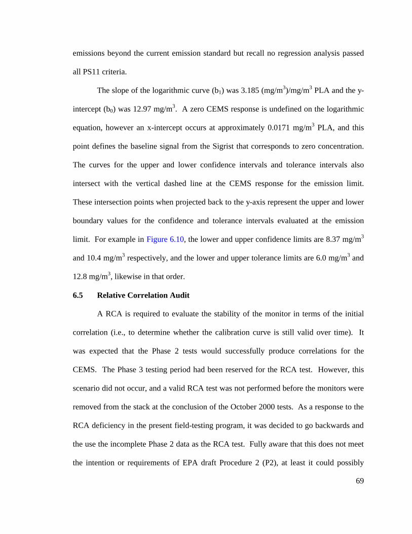
69
emissions beyond the current emission standard but recall no regression analysis passed
all PS11 criteria.
The slope of the logarithmic curve (b1) was 3.185 (mg/m3)/mg/m3 PLA and the y-
intercept (b0) was 12.97 mg/m3. A zero CEMS response is undefined on the logarithmic
equation, however an x-intercept occurs at approximately 0.0171 mg/m3 PLA, and this
point defines the baseline signal from the Sigrist that corresponds to zero concentration.
The curves for the upper and lower confidence intervals and tolerance intervals also
intersect with the vertical dashed line at the CEMS response for the emission limit.
These intersection points when projected back to the y-axis represent the upper and lower
boundary values for the confidence and tolerance intervals evaluated at the emission
limit. For example in Figure 6.10, the lower and upper confidence limits are 8.37 mg/m3
and 10.4 mg/m3 respectively, and the lower and upper tolerance limits are 6.0 mg/m3 and
12.8 mg/m3, likewise in that order.
6.5 Relative Correlation Audit
A RCA is required to evaluate the stability of the monitor in terms of the initial
correlation (i.e., to determine whether the calibration curve is still valid over time). It
was expected that the Phase 2 tests would successfully produce correlations for the
CEMS. The Phase 3 testing period had been reserved for the RCA test. However, this
scenario did not occur, and a valid RCA test was not performed before the monitors were
removed from the stack at the conclusion of the October 2000 tests. As a response to the
RCA deficiency in the present field-testing program, it was decided to go backwards and
the use the incomplete Phase 2 data as the RCA test. Fully aware that this does not meet
the intention or requirements of EPA draft Procedure 2 (P2), at least it could possibly

70
demonstrate the stability of the Phase 3 calibration curves between March and October
2000.
According to Procedure 2, the RCA measurements are regarded as consistent with
the current calibration relation if at least 75% of a minimum number of 12 sets of
CEMS/M5i measurements fall within the tolerance interval at ± 25% of the emission
limit established during the PS11 initial correlation test. Since the Durag did not generate
valid data during Phase 2, it cannot take part in the current RCA illustration, but at least
seven M5i/CEMS measurements were legitimate for the ESA and Sigrist monitors. Note:
this RCA test was not completed in strict accordance with the P2 requirements, especially
since 12 M5i/CEMS measurements are required at the three levels of PM concentration
for the facility, and only seven measurements were used, which barely represented the
Level 1 (low) range. Furthermore, the RCA data were collected in the time period
occurring before the calibration curve data were collected; in other words, the audit test
preceded the correlation test.
Figure 6.12 is a graph of the ESA Phase 2 data superimposed over the ESA Phase
3 linear calibration curve. Figure 6.13 is a graph of the Sigrist Phase 2 data superimposed
over the Sigrist Phase 3 logarithmic calibration curve. In both figures, the Phase 3 data
have been removed, but the confidence and tolerance intervals are retained. As is evident
from the ESA figure, six out of seven or approximately 85% of the data points fell within
the tolerance intervals. In the Sigrist figure, only four out of seven or approximately 60%
of the data points fell within the tolerance intervals. Realize however, that the Sigrist
Phase 3 logarithmic curve also did not pass the PS11 correlation criteria.

71
6.6 Inter-instrument Comparisons Between CEMS
To help understand the relationship between the beta-gauge technology and the
light-scattering technology, three correlation analyses between the analyzers were
conducted to discover how well they were responding to similar conditions in the stack.
Precisely five days of 1-hour CEMS measurements or about 120 data points per monitor
were correlated. Figure 6.14 shows the Durag versus the ESA correlation for the linear
trend line. The product-moment correlation R-squared value was 0.917, indicating a high
correlation between the beta-gauge monitors. Figures 6.15 and 6.16 show the Durag
versus the Sigrist and the ESA versus the Sigrist, respectively. For these correlations the
linear and logarithmic trend lines are both shown. The product-moment correlation R-
squared values for linear trend lines were close to 0.707 and 0.645, and for the
logarithmic trend lines, the R-squared values were 0.819 and 0.876, respectfully. . The
linear relationships were not very strong between the beta-gauge instruments and the
Sigrist instrument. The fact that the logarithmic approach was somewhat better is no
surprise since the PS11 regression analysis suggested that a logarithmic fit defined the
relationship between Sigrist and the gravimetric M5i.
There is one additional area that can be used to illustrate the performance of the
CEMS. Recall that the ionizing wet scrubbers (IWS) are the final air pollution control
devices the flue gas enters before exiting the sack. To demonstrate the reliable operation
and sensitivity between the monitors, a benefit can be taken from a relationship that
exists between the electric field strength across the collecting plates of the IWS and the
PM removal efficiency. As will be shown, particulate emissions increase during the flush
cycle due to reduced collection efficiency of the IWS.

72
Remember that two identical IWS were located in series, and both devices
operated on a continuous basis. However, alternating every 4 hours, each IWS goes into
a water flush cycle to remove the build-up of PM on the plates and other IWS surfaces.
During the flush cycle on one of the IWS, the voltage drops to zero, and the plates are
flushed with re-circulated rinse water for about 5-minutes. It is possible that emissions
might slightly increase during this time period because one IWS is offline, and also some
of the captured particles can become re-entrained in the gas stream during the wash cycle.
Figures 6.17 and 6.18 show the PM concentration as measured by the Durag and
ESA, and the Sigrist monitors, respectively, versus the waste feed rates and the IWS zero
voltage conditions during October 16, 2000. On both graphs, the IWS zero voltage state
is represented by large solid rectangles. The left hand y-axis represents the CEMS
response; the right hand y-axis represents the waste feel rate and the zero IWS voltage
condition. Time is represented along the x-axis. Notice in these figures that each
monitor detected the increase in PM every time an IWS went into a wash cycle as
represented by the voltage drop to zero and the ensuing increase in the response of the
monitors. These spikes are especially evident between 8:00 and 12:00, than they are
between 16:00 and 21:00 whereupon the waste feed rates had been increased. The
response of the monitors matched the increase in the waste feed rates. Around 18:00 the
waste feeds were briefly stopped. This event coincided with the wash cycle of IWS-2,
and as reveal, the monitors responded appropriately.
Generally, the overall magnitude of the spike for each monitor should have been
smaller for IWS-1, as compared with IWS-2. Since IWS-2 is down-stream of IWS-1, it
captures a fraction of the increased particle emissions that escaped IWS-1 during its

73
cleaning cycle. On the other hand, any particles emitted during the IWS-2 cleaning cycle
went directly into the stack and were measured by the CEMS. However, this observable
fact was not represented in these two figures, and this was almost certainly related to the
fact that the wastes feed rates were not constant during the time period when the IWS
went into a wash cycle.

74
CHAPTER 7
CONCLUSIONS/SUMMARY
The uses of CEMS are increasingly being required by regulations to ensure that
the source is meeting its permitted emission rates and for verifying that the mandated
reduction of emissions are eventually being achieved. There is a critical need for the
real-time quantification of emissions from the stack gas of waste incinerators. However,
it is equally important that these CEMS provide accurate and reliable emission
information. This study evaluated the results of three commercially available PM CEMS
at a hazardous waste incinerator that routinely treats many different types of liquid,
aqueous, and solid wastes. The ability to treat these various wastes simultaneously plus
the fact that the flue gas of the incinerator was constantly near the saturated moisture
condition presented a major challenge for the individual CEMS to establish a single,
acceptable correlation relationship.
Three sets of reference method tests were conducted during a 10-month time
period. The set of tests called Phase 1 and Phase 2 were not sufficient to achieve a
suitable calibration curve according to U.S. EPA draft PS11 and P2 criteria. Phase 1
testing was conducted as a learning experience and was not really expected to produce
reliable data; still, the Phase 2 testing was also unsuccessful because it was not possible
to generate the full range of emissions necessary to produce the calibration curve at the
current emission standard. However, the primary reason for the failure of Phase 2 to
meet the EPA criteria cannot be attributed to the operation of the PM CEMS. Rather, it

75
was not possible for the facility to achieve the range of emissions needed due to the lack
of a sufficient variation in the waste characteristics.
The Phase 3 correlation tests did meet the criteria of simultaneous M5i/CEMS
measurements over the full range of operations for the facility. The CEMS also operated
under reasonable normal facility operations, and there was 100% recovery of data from
the three monitors. A total of 19 successful M5i/CEMS tests were used to generate the
calibration curves. According to PS11 criteria, the Durag and ESA produced a valid
linear calibration curve. For the Sigrist, a logarithmic calibration curve came closest to
passing PS11 criteria, though acceptable values for the confidence and tolerance interval
percent were not achieved. Therefore, Sigrist did not pass the correlation test
requirements of PS11.
Extrapolation of the calibration curve is limited to 125% of the highest measured
PM CEMS concentration. The upper and lower confidence intervals and tolerance
intervals are depicted over the entire range of the calibration curve. The confidence
intervals are always narrower than the tolerance intervals, and both are narrowest at the
central region of the sample data, which actually specifies the mean value of the
regression curve. As the CEMS values along the x-axis increase further outside the range
of the actual data, the confidence and tolerance intervals also spread outwardly. The
confidence intervals are evidently more sensitive to increasing values beyond the range of
the sample data. It is possible that the confidence intervals could expand and intersect the
boundaries of the tolerance intervals. Again, this demonstrates the erroneous result of
making inference beyond the observed data.

76
A series of RCA tests must be performed at 6-month intervals to assure the
continued validity over time of the initial calibration curve. In the project site-plan, the
Phase 3 time period was reserved for these tests. Since the Phase 2 testing had basically
turned out to be unproductive, the Phase 3 testing period that had been reserved for the
RCA tests was used to generate the calibration relationships. Nonetheless to provide
information on the long-term stability and accuracy of the calibration curves, the seven
valid M5i/CEMS data points that had been collected from Phase 2 were used as a pseudo
RCA test. About 6-months had intervened between Phase 2 and 3, and different wastes
had been treated during each of the time periods. (The Durag monitor could not play a
part in this trial because it did not produce reliable data during Phase 2.) From this
examination though, it seems that at least the ESA Phase 2 data was consistent with the
ESA Phase 3 calibration curve according to relaxed or pseudo RCA criteria. In contrast,
the Sigrist Phase 2 data did not appear to be consistent with the Sigrist Phase 3 calibration
curve. It should be recalled that one of the disadvantages of light-scattering as a
detection principle is the possibility of a non-linear response to changing particle
characteristics, like size distribution or refractive index. When very dissimilar wastes are
incinerated, it is probable that the output response of a light-scattering monitor cannot be
represented by a single calibration curve. Other test programs, where a consistent waste
was incinerated have shown that the Sigrist passed the EPA PS11 requirements.
The proper functioning of air dilution/heating systems are vital in sampling moist
flue gas to ensure that the dew point of the gas sample is not reached, consequently
resulting in condensation before the sample actually passes through the analyzer. It was
not possible to know precisely the moisture condition of the gas sample since none of

77
these monitors measured the dew point of the flue gas as it was analyzed. It is believed
that the Durag did not produce reliable data during Phase 1 and 2 because the instrument
could not handle the moisture conditions of the stack gas. The dilution-air chiller for the
monitor was undersized during the system installation, and numerous malfunctions were
also associated with the purge-air cycle trapping condensed water and wetting the filter
tape. Typically, the light-scattering instrument by using a photocell design encounters
fewer problems with condensation because the gas sample does not come into direct
surface contact with the analyzer. Yet, there are no means to determine if water droplets
are entrained in the gas sample. On the other hand for the beta-gauge instrument, the gas
sample goes through the filter tape, which can undergo wetting if the gas sample is near
the dew point and the filter mechanism not is adequately heated. In rating the
instruments with respect to the sampling lines and peripherals like the ring pipe
insulation, it was felt that the Sigrist had been much better designed than the two beta-
gauge instruments. Moreover, the Sigrist had fewer moving part; therefore, it
experienced fewer problems and required less maintenance than the beta-gauge monitors
during the shakedown and operation periods.
The ESA monitor was considered superior to the Durag monitor during episodes
of high particle mass loading of the filter paper. While sampling flue gas, both
instruments could detect a vacuum error, but in doing so, the ESA could immediately
terminate the measuring cycle and then analyze the sample; where as, the Durag could
only generate an error flag to indicate that the sampling cycle value was a suspect
measurement. Furthermore, the ESA monitor always maintained isokinetic sampling

78
conditions, which are the requirements of reference M5i testing. Alternatively, the Durag
and Sigrist always analyzed the flue gas above the isokinetic sampling conditions.
Questions have been raised regarding the batch type beta-gauge devices, which
have only one sampling head, such that they only measure a fraction of the time (e.g.,
sampling 5 minutes during each 10-minute cycle). This field study showed that the beta-
gauge monitors still could satisfy the PS11 criteria at the TSCA incinerator, in spite of
only sampling the flue gas less than about 60% of the time relative to the reference
method. At the present, manufacturers of beta-gauge monitors are including a second
sampling head to allow the batch samplers to meet the continuous monitoring
requirements of the MACT standards. It is uncertain, whether EPA will approve the
single sampling headed instruments used in this study, as meeting the requirement of
continuous monitoring specified in PS11.
The primary advantage of the beta-gauge technology is that it is insensitive to
changes in PM properties. Additionally, both beta-gauge monitors correlated highly
between one another based on the comparison of hourly averages. While the beta-gauge
samplers were shown to have met the PS11 criteria during the Phase 3 tests, the RCA
tests have not yet been conducted to provide information on the long-term stability and
accuracy of the initial calibration curve. Based on the tests conducted in this study, the
most critical part of the certification procedure for the CEMS was that the correlation test
be conducted over the full range of operation for the facility, especially at or near the
emission standard. This may require the operators of the source to operate in a way that
is exceeding the PM emission limit during the correlation test. Furthermore, the
minimum number of 15 M5i paired tests may be insufficient to generate the calibration
79
curve for PS11. In reality, an average of 50 to 75 M5i tests may be required to be
successful, especially in situations where very different types of hazardous and non-
hazardous wastes are being incinerated.
The following statements summarize the lessons learned from this field study:
• Careful planning and selection of the appropriate waste feeds and incinerator
operating conditions for generating a wide range of PM emissions are crucial to
achieve a successful correlation test.
• The beta-gauge instrument that reported emissions on a dry basis was sufficiently
challenged by moisture condensation from the saturated flue gas sample prior to
the volume measurement. Numerous operational problems were encountered
with both beta-gauge instruments, but these difficulties were eventually resolved
through vendor intervention. The light-scattering device required only minor
maintenance, and it operated trouble-free throughout the field demonstration.
• There were no apparent effects from trace levels of low-level radioactive
emissions on the determination of PM concentration by the beta gauge monitors.
• Paired train data at concentrations less than 10 mg/dscm had difficulty meeting
the relative standard deviation criteria for precision.
• The beta gauge monitors passed all three minimum specifications for the
correlation test criteria.
• The light-scattering device failed two of the three minimum specifications for the
correlation test. It may be necessary to generate more than one calibration curve
depending on the waste feed type.

80
REFERENCES

81
LIST OF REFERENCES
Clap saddle, C and Trenholm, A. "Current Knowledge of Particulate Matter (PM) Continuous Emission Monitoring". Prepared by Midwest Research Institute for EPA Office of Air Quality Planning and Standards. Research Triangle Park, NC. EPA-454/R-00-039. September 8, 2000. Conner, W.D. and Hodkins, J.R. "Optical Properties and Visual Effects of Smoke-Stack Plumes". Public Health Service/National Center for Air Pollution Control. Cincinnati, OH. NTIS Publication Number PB999AP30. 1967. Conner, W. D. "Measurement of Opacity and Mass Concentration of Particulate Emissions by Transmissometry". National Environmental Research Center. Research Triangle Park, NC. EPA-650/2-74-128. 1974. Conner, W.D., Knapp, K.T., and Nader, J.S. "Applicability of Transmissometers to Opacity Measurement of Emissions - Oil-fired Power Plants and Portland Cement Plants". Environmental Sciences Research Lab. Research Triangle Park, NC. EPA 600/2-79-188. 1979. Conner, W.D. and White, N. "Comparative Study of Plume Opacity Measurement Methods". Environmental Sciences Research Lab. Research Triangle Park, NC. EPA600/2-80-001. 1980. Durag Service Manual: (F-904 K-PLC). Durag Incorporated Elecktronik Co. 105 Kollaustrasse. Hamburg, Germany. 1999 (unpublished). Energy and Environmental Research Corporation (EERC). "Particulate Matter Continuous Emission Monitoring Systems Field Study, Site-Specific Quality Assurance Test Plan". Prepared for the U.S. Department of Energy and Bechtel Jacobs Company. Revision 2. July 20, 1999 (unpublished). EPA (U.S. Environmental Protection Agency), "CEMS Demonstration Announcement". Federal Register: Vol. 61, No. 39, February 27, 1996. EPA (U.S. Environmental Protection Agency), "Hazardous Waste Combustors; Revised Standards; Proposed Rule: CEMS Demonstration Announcement". Federal Register: Vol. 61, No. 39, April 19, 1996. EPA (U.S. Environmental Protection Agency), "Total Mercury and Particulate Continuous Emission Monitoring Systems; Measurement of Low Level Particulate Emissions; Implementation at Hazardous Waste Combustors; Proposed Rule". Federal Register: Vol. 62, No. 249, December 30, 1997.

82
EPA (U.S. Environmental Protection Agency), "Particulate Matter CEMS Demonstration: DuPont Experimental Station On-Site Incinerator", EPA 68-D2-0164. February 12, 1997. EPA (U.S. Environmental Protection Agency), "Procedure 2: Quality Assurance Requirements for Particulate Matter Continuous Emission Monitoring Systems", Office of Solid Waste, Washington, DC: Work-in-Progress (11-3-98). EPA (U.S. Environmental Protection Agency), "Performance Specification 11: Specifications and Test Procedures for Particulate Matter Continuous Emission Monitoring Systems in Stationary Sources", Office of Solid Waste, Washington, DC: Work-in-Progress (11-3-98). EPA (U.S. Environmental Protection Agency), "Final Technical Support Document for HWC MACT Standards; Volume IV; Compliance with the HWC MACT Standards" EPA 68-D2-0164 and 68-W7-0029. July 1999. EPA (U.S. Environmental Protection Agency), "NESHAPS: Final Standards for Hazardous Air Pollutants for Hazardous Waste Combustors, Final Rule", Federal Register: Vol. 64, No. 189, September 30, 1999. EPA (U.S. Environmental Protection Agency), "Method 5i: Determination of Low Level Particulate Matter Emissions from Stationary Sources", CFR 40 Part 60, Appendix A. Washington DC: July 1, 2000. EPA (U.S. Environmental Protection Agency), "NESHAPS: Final Standards for Hazardous Air Pollutants for Hazardous Waste Combustors", Federal Register: Vol. 65, No. 132, July 10, 2000. ESA Service Manual: (Beta 5M Monitor). Environnement S.A. 111 Boulevard Robespierre. Poissy, France. 1998 (unpublished). Jahnke, J.A. Continuous Emission Monitoring. Van Nostrand Reinhold. New York, NY. 1993. Lilly Project Report: "Particulate Matter CEMS Test, Volume 1". Prepared by Focus Environmental Inc. for Eli Lilly and Co. Indianapolis, IN. September 1998. Lilly Project Report: "Addendum to September 1998 PM CEMS; Phase II". Prepared by Focus Environmental Inc. for Eli Lilly and Co. Indianapolis, IN. April 30, 1999. Lodge, James P. Jr. (Ed.). Methods of Air Sampling and Analysis (Third Edition). CRC Press. Boca Raton, FL. 1988.

83
Sigrist Service/Instruction Manuals: CTNR Light-scattering Monitor. Sigrist-Photometer AG. 1 Hofurlistrasse. Ennetburgen, Switzerland. 1998 (unpublished). Roberson, R.L. "Status of EPA's Continuous Particulate Mass (PM) Monitor Demonstrations". Presented at the 1997 EPRI CEM User Group Meeting. Denver, CO. May 14-16, 1997. Wark, K., Warner, C.F. and Davis W.T. Air Pollution: Its Origin and Control. Addison-Wesley Longman, Inc. Menlo Park, CA. 1998.

84
APPENDIX

85
Appendix A
Tables Discussed in Body of Report

86
Table 2.1 Summary of PM CEMS Performance Characteristics (without outliers) for the DuPont Waste Incinerator*
CEMS Detection Principal
M5i Testing Period
Correlation Coefficient
> 0.90
Confidence Interval < 10%
Tolerance Interval < 25%
Pre-test 0.554 26.2 38.3
First 0.927 7.3 23.7 ESA beta
Second 0.985 5.7 15.5
Pre-test 0.691 27.3 32.1
First 0.968 5.1 20.0 Verewa beta
Second 0.961 8.0 21.7
Pre-test 0.715 21.7 36.0
First 0.952 7.2 17.2 Durag optical
Second 0.972 6.9 18.8
Pre-test 0.708 22.1 36.4
First 0.966 5.2 21.2 ESC optical
Second 0.978 6.2 16.9
Pre-test 0.644 25.5 40.0
First 0.936 7.1 28.7 Sigrist optical
Second 0.951 9.2 24.9 * Analysis based on linear regression
Table 2.2 Summary of PM CEMS Performance Characteristics (without outliers) for the Eli Lilly Waste Incinerator
CEMS Detection Principal
M5i Testing Period
Correlation Coefficient
> 0.90
Confidence Interval < 10%
Tolerance Interval < 25%
Phase I* 0.31 3.1 5.5 ESA beta
Phase II* 0.99 2.6 9.1
Phase I* 0.73 1.7 2.4 Sigrist optical
Phase II** 0.97 6.7 24.3
* Analysis based on linear regression; ** Analysis based on logarithmic regression

87
Table 3.1 Typical Flue Gas Conditions at the Sampling Location
Under Normal Incinerator Operating Conditions
Description Condition Units
Temperature 175 -185 oF
Static Pressure - 0.25 inches H20
8,000 – 9,000 dscf Flow Rate
17,000 – 19,000 acfm
Velocity 18 – 20 fps
O2 9 – 11 %
CO2 5 – 8 %
Moisture 45 – 55 %
0.005 – 0.030 gr/dscf @ 7% O2 PM Loading (front-half) 10 – 70 mg/dscm @ 7% O2
(Adapted from: EERC, 1999)

88
Table 3.2 Incinerator Process Parameters Monitored
During the PM CEMS Demonstration
Description Range* Units
Stack Barometric Pressure 400 – 800 mm Hg
Stack Temperature 0 – 400 oF
Combustion Gas Velocity 0 – 35 fps
O2 Monitor 1 0 – 25 % dry
O2 Monitor 2 0 – 25 % dry
IWS-1 Voltage 0 – 40,000 volts
IWS-2 Voltage 0 – 40,000 volts
Primary Feed Rate 0 – 1000 lbs/hr
Aqueous Feed Rate 0 – 500 lbs/hr
Secondary Feed Rate 0 – 1000 lbs/hr
Solids Feed Rate 0 – 1000 lbs/hr
Solids Scale Reading 0 – 100 lbs
NG to Secondary Burner 0 – 21,000 scfh
NG to Primary Burner 0 – 11,000 scfh
CO2 Monitor 1 0 – 20 % dry
CO2 Monitor 2 0 – 20 % dry
(Adapted from: EERC, 1999); *Min-max range of detector.

89
Table 4.1 Input/Output Signal Requirements for the Purpose of Data Logging*
Analog None
Input Digital
Start calibration – unit is looking for a contact closure (no voltage) from the data logger for a minimum of 2 seconds duration. This will initiate the calibration routine. Dust concentration (mg/N-m3) – range is programmable. Dust concentration – isolated (4 –20 mA). Analog Mass of dust on filter tape (mg) – range is fixed at 10 mg. Filter tape torn error Measuring range error – over range. Sample volume error – total volume deviates from set point. Vacuum error – probe or filter tape plugged. Zero – results from zero test of calibration.
Durag F-904K
Output
Digital
Span – results from upscale calibration.
Input Analg/Digital None Dust concentration (mg/N-m3) – range is programmable. Dust concentration – isolated (4-20 mA). Geiger counts (counts/sec). Intake volume (N-liters). Stack gas velocity (m/sec). Stack temperature (oC). Venturi static pressure (mbar). Venturi tube temperature (oC).
Analog
Error alarm code number. General error alarm.
ESA Beta 5M Output
Digital Single relay contact for "Standby" – i.e. for calibration mode.
Input Analg/Digital None Dust concentration - isolated (4 –20 mA). Relay 1, 2, and 3 are used to signal range information. Dust concentration low range response (mg/m3 PLA).* Analog
Dust concentration high range response (mg/m3 PLA).* Range 4 active; relays 1, 2 & 3 open. Range 3 active; relays 3 close; relays 1 & 2 open. Range 2 active; relays 2 close; relays 1 & 3 open. Range 1 active; relays 1 close; relays 2 & 3 open. Relay 4 close – instrument in service/calibration mode.
Sigrist CTNR Output
Digital
Relay 5 close – instrument error or malfunction. See error code on monitor digital display.
(Adapted from: EERC, 1999); *Sigrist monitor operation only one set of ranges is active

90
Table 4.2 Summary of PM CEMS Sampling Characteristics
Description Durag ESA Sigrist
Flow Rate Sampling Condition
Slightly above average stack
velocity
Maintained isokinetic
automatically
Slightly above average stack
velocity
Sampling Protocol Dry
Dilution (air) & Heated Probe
Heated Probe (only)
Heated Probe (only)
Probe Temperature 120 oC 120 oC 160 oC
Gas Sampling Volume and/or
Dilution Volume
400 L 135 L ~ 300 L n/a
Reporting Conditions Dry,
20 oC & 1013 mbar
Wet, 0 oC &
1013 mbar
Wet, 160 oC &
1013 mbar
Concentration Sampling Range
(see also Table 5.1)
0 - 100 mg/dscm
0 – 100 mg/Nm3
0 – 50 mg/m3 PLA
Measuring Cycle 10 - 12 min 10 - 12 min ~ 1 sec
Sampling Cycle 5 – 7 min 5 - 7 min Continuous

91
Table 5.1 Summary of CEMS Measuring Ranges and Equations for Conversion between Milliamp and Concentration
Instrument Concentration Range Linear Equation
Durag (mg/dscm) 0 – 100 Y = 6.25X – 25
0 – 70 Y = 4.375X – 17.5 ESA (mg/Nm3) 0 – 100 Y = 6.25X – 25
0 – 0.05 Y = 0.003125X – 0.0125
0 – 0.2 Y = 0.0125X – 0.05
0 - 1 Y = 0.0625X – 0.25
Sigrist low-range*
(mg/m3 PLA)
0 - 30 Y = 1.875X – 7.5
0 – 0.1 Y = 0.00625X – 0.025
0 – 1 Y = 0.0625X – 0.25
0 – 5 Y = 0.3125X – 1.25
Sigrist high-range** (mg/m3 PLA)
0 – 50 Y = 3.125X – 12.5
*Sampling range during Phase 1; **Sampling range during Phase 2 and 3. Y = Concentration; X = milliamp signal.

92
Table 6.1 Estimation of Precision and Rejection of Statistical Outliers
for Phase 2 M5i PM Concentration Data
PM Concentration
(mg/dscm) @ 7% O2
Date Waste Types
Run No.*
Train-1 Train-2
Ave PM
Conc
RSD (%)
MPC (%) Result
Natural Gas R13 1.25 2.96 2.11 40.6 23.2 Fail
Natural Gas R14 1.87 0.807 1.34 39.7 24.4 Fail
Combination Solids R15 10.9 8.46 9.68 12.6 10.5 Fail
24-Mar
Combination Solids R16 7.13 7.85 7.49 4.81 14.2 Pass
Natural Gas R17 1.19 0.991 1.09 9.12 24.8 Pass
Combination Solids & Soil Solids R18 3.89 4.66 4.28 9.01 19.5 Pass
Combination Solids & Soil Solids R19 5.74 5.84 5.79 0.86 17.0 Pass
25-Mar
Combination Solids & Soil Solids R20 3.31 3.09 3.20 3.44 21.3 Pass
Natural Gas R21 0.811 -0.677 0.07 1110 No-limit Pass
Combination Solids & Soil Solids R22 15.0 14.5 14.75 1.69 10.0 Pass
Soil Solids R23 1.94 3.77 2.86 32.0 21.9 Fail
26-Mar
Soil Solids R24 -3.69 1.60 -1.05 -253 N/A Fail
*The Phase 1 data was not included, in this paper; but to maintain consistency with the Method 5i laboratory report, the AES numbering scheme for the runs was maintained throughout this paper. RSD = Relative Standard Deviation; MPC = Minimum Precision Criteria.

93
Table 6.2
Summary of Waste Feed Categories, Ash Content, and Feed Rates for Phase 3
Waste Description lb/hr
Min 140
Max 340 Primary
Ave 260
Min 110
Max 310 Secondary
Waste oils and organics (ash content 0.1 % by weight)
Ave 230
Min 130
Max 350 Aqueous Nitric acid with depleted uranium
and combination bulk liquids (ash content 6.9 % by weight)
Ave 270
Min 115
Max 160 Solid I Repackaged solids with PCBs (ash content 5.7% by weight)
Ave 140
Min 260
Max 370 Solid II Spent carbon (ash content 5.4% by weight)
Ave 330
Table 6.3 Three Different Levels of PM Concentration
Over Incinerator Operations for Phase 3
Range (mg/dscm)* Level Range Interval*
(mg/dscm) No.
Runs Method 5i
Runs MIN MAX
%
1 (low) 0-50% x < 39.2 5 R26, R36, R37,
R38, R44 1.8 22.6 26.3
2 (medium) 25-75% 19.6 > x > 58.7 10
R27, R28, R32, R33, R34, R35, R39, R41,
R42, R43 25.3 38.4 52.6
3 (high) 50-100% x > 39.2 4 R29, R30,
R31, R40 39.3 78.3 21.1
* PM concentrations (mg/dscm) are also reported at 7% oxygen.

94
Table 6.4 Estimation of Precision and Rejection of Statistical Outliers
for Phase 3 M5i PM Concentration Data
PM Concentration
(mg/dscm) @ 7% O2
Date Waste Types
Run No.*
Train-1 Train-2
Ave PM
Conc
RSD (%)
MPC (%) Result
Primary/Secondary & Aqueous R26 22.8 22.3 22.55 1.11 10.0 Pass
Primary/Secondary & Aqueous R27 32.4** 33.3 32.85 1.37 10.0 Pass
Primary/Secondary & Aqueous R28 23.5 27.1** 25.30 7.11 10.0 Pass
Primary/Secondary & Aqueous R29 51.7 50.9 51.30 0.78 10.0 Pass
19-Oct
Primary/Secondary & Aqueous R30 80.0 76.6** 78.30 2.17 10.0 Pass
Aqueous R31 54.7 48.3 51.50 6.21 10.0 Pass
Primary/Secondary, Aqueous & Solid I R32 32.4 29.9 31.15 4.01 10.0 Pass
Primary/Secondary, Aqueous & Solid I R33 26.7 26.0 26.35 1.33 10.0 Pass
Primary/Secondary, Aqueous & Solid I R34 24.5 27.2 25.85 5.22 10.0 Pass
20-Oct
Primary/Secondary, Aqueous & Solid I R35 38.9 37.8 38.35 1.43 10.0 Pass
Primary/Secondary & Solid II R36 5.55 5.21 5.38 3.16 17.7 Pass
Primary & Solid II R37 8.65 8.26 8.46 2.31 12.6 Pass 21-Oct
Primary/Secondary & Solid II R38 13.7 13.5 13.60 0.74 10.0 Pass

95
Table 6.4 (continued)
PM Concentration (mg/dscm) @
7% O2 Date Waste
Types Run No.*
Train-1 Train-2
Ave PM Conc
RSD (%)
MPC (%) Result
Primary/Secondary, Aqueous & Solid II R39 33.6 33.1 33.35 0.75 10.0 Pass
Primary/Secondary, Aqueous & Solid II R40 41.0 37.6 39.30 4.33 10.0 Pass
Primary/Secondary, Aqueous & Solid II R41 31.8 31.4 31.60 0.63 10.0 Pass
Primary/Secondary, Aqueous & Solid II R42 31.9 31.8 31.85 0.16 10.0 Pass
22-Oct
Primary/Secondary & Aqueous R43 34.9 33.5 34.20 2.05 10.0 Pass
Primary/Secondary R44 1.85 1.77 1.81 2.21 23.7 Pass
24-Oct
Primary/Secondary R45 2.11 1.25 1.68 25.60 23.9 Fail
*Run 25 was not reported; it was discontinued during the Method 5i sampling test because condensed moisture in the train exceeded the capacity of the impinges and liquid water saturated the silica gel. ** The Method 5i train operator was unable to maintain an isokinetic sampling rate to within 10% of the true isokinetic rate. RSD = Relative Standard Deviation; MPC = Minimum Precision Criteria.

96
Table 6.5 CEMS and M5i Phase 3 Data
Adapted for Use in the Correlation Tests
Durag ESA Sigrist
Run No. CEMS
(mA) M5i
(mg/dscm) CEMS
(mg/Nm3) M5i
(mg/Nm3)
CEMS (mg/m3 PLA)
M5i (mg/m3)
R26 5.581 16.38 8.67 9.151 0.253909 5.771 R27 6.583 23.61 10.30 13.41 0.511662 8.459 R28 5.891 19.44 9.21 10.61 0.239761 6.692 R29 8.654 39.48 19.69 21.70 1.425907 13.69 R30 9.457 61.42 29.21 33.59 3.218443 21.18 R31 8.433 41.26 20.95 23.63 0.529626 14.90 R32 6.579 25.10 12.50 14.15 0.343226 8.830 R33 5.834 21.00 10.55 12.25 0.228386 7.710 R34 5.848 20.89 10.31 12.00 0.367018 7.564 R35 6.894 30.35 10.86 17.29 0.544798 10.90 R36 4.305 3.945 0.55 2.256 0.011863 1.423 R37 4.525 6.708 3.13 3.786 0.054513 2.387 R38 4.415 10.78 4.52 6.152 0.031211 3.880 R39 6.616 27.11 12.58 15.25 0.383198 9.617 R40 6.373 31.21 12.99 17.36 0.599869 10.93 R41 6.353 25.07 10.75 13.93 0.286351 8.785 R42 6.659 25.37 11.36 14.05 0.320300 8.862 R43 6.916 27.04 11.96 15.16 0.305484 9.558 R44 4.475 1.325 0.08 0.7578 0.018696 0.4779 R45* 4.421 1.305 0.14 0.7336 0.017807 0.4626 * Run did not pass Procedure 2 RSD% criteria.

97
Table 6.6 Summary of Durag Phase 3
PS11 Calibration Results
Linear Logarithmic Polynomial Description
y = b1x + b0 y = b1Ln(x) + b0 y = b2x2 + b1x + b0
PS11 Correlation r-value = 0.964 0.952 0.963
b2 = - - 0.2000
b1 = 9.548 59.90 6.881 Regression Coefficients
b0 = -36.42 -85.10 -27.94
Maximum Predicted Concentration,
ymax 125% (mg/dscm) =
at xmax 125% (mA) = 10.82
66.90 57.55 69.95
CEMS Response Required to Report
Emission Standard (mA) =
Emission Standard at Condition of CEMS
(mg/dscm) = 26.42
6.58 6.44 6.62
Confidence Interval (%) at Emission Standard = 6.9 8.0 9.2
Tolerance Interval (%) at Emission Standard = 23.2 26.9 24.4
Comparison between Linear and Polynomial
Best-fit Curves
F1f value = 4.49
Observed (S) ratio = 0.31
The linear equation is the best-fit curve.

98
Table 6.7 Summary of ESA Phase 3 PS11 Calibration Results
Linear Logarithmic Polynomial Description
y = b1x + b0 y = b1Ln(x) + b0 y = b2x2 + b1x + b0
PS11 Correlation r-value = 0.985 0.761 0.985
b2 = - - -0.0028
b1 = 1.1050 4.3592 1.1812 Regression Coefficients
b0 = 1.2764 4.8684 0.9033
Maximum Predicted Concentration,
ymax 125% (mg/Nm3) =
at xmax 125% (mg/Nm3) = 36.51
41.62 20.55 40.29
CEMS Response Required to Report
Emission Standard (mg/Nm3) =
Emission Standard at Condition of CEMS
(mg/Nm3) = 14.87
12.31 9.93 12.18
Confidence Interval (%) at Emission Standard = 4.4 16.8 5.4
Tolerance Interval (%) at Emission Standard = 14.8 55.9 15.4
Comparison between Linear and Polynomial Best-fit Curves
F1f value = 4.49
Observed (S) ratio = 0.41
The linear equation is the best-fit curve.

99
Table 6.8 Summary of Sigrist Phase 3
PS11 Calibration Results
Linear Logarithmic Polynomial Description
y = b1x + b0 y = b1Ln(x) + b0 y = b2x2 + b1x + b0
PS11 Correlation r-value = 0.818 0.908 0.895
b2 = - - -2.7715
b1 = 5.5636 3.1848 14.243 Regression Coefficients
b0 = 5.6785 12.965 3.3666
Maximum Predicted Concentration,
ymax 125% (mg/m3) =
at xmax 125% (mg/m3 PLA) = 4.023
28.06 17.40 15.81
CEMS Response Required to Report Emission
Standard (mg/m3 PLA) =
Emission Standard at Condition of CEMS
(mg/m3) = 9.38
0.6652 0.3243 0.4641
Confidence Interval (%) at Emission Standard = 14.8 10.8 13.4
Tolerance Interval (%) at Emission Standard = 49.5 36.1 39.4
Comparison between Linear and Polynomial Best-fit Curves
F1f value = 4.49
Observed (S) ratio = 12.2
The logarithmic equation is the best-fit curve.

100
Appendix B
Figures Discussed in Body of Report

101
Figure 3.1: Aerial photograph of the TSCA Incinerator demonstration area. Note: the picture was taken during 1995; since that time, additional buildings
have been added to the facility grounds.

102
Figure 3.2: Overall schematic of the TSCA Incinerator process systems
and air pollution control equipment. (Adapted from: EERC, 1999).

103
Figure 4.1: Front view of Durag F-904 K beta-gauge monitor. General description: The measurement and control assembly are enclosed in a sealed cabinet. The following components are located in the cabinet: (1) Three-way ball valve - entry for flue gas sample; (2) Filter adapter - contains beta source and Geiger- Müller detector; (3) Filter tape pad roll; (4) Peristaltic pump; (5) Sample gas chiller; (6) Keyboard and display; (7) Main switch; (8) Supply filter tape reel; (9) Grip; (10) Filter; (11) Sample gas pump; (12) Cabinet base. Source: Durag Service Manual: (F-904 K-PLC). Durag Incorporated Elecktronik Co. 105 Kollaustrasse. Hamburg, Germany. 1999 (unpublished).
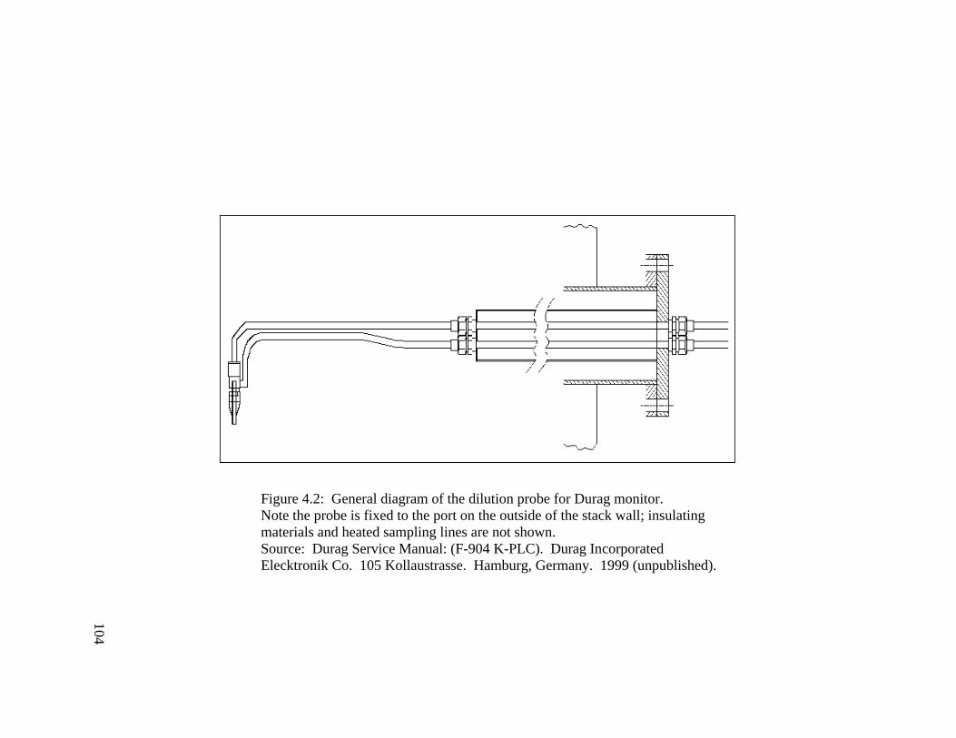
Figure 4.2: General diagram of the dilution probe for Durag monitor. Note the probe is fixed to the port on the outside of the stack wall; insulating materials and heated sampling lines are not shown. Source: Durag Service Manual: (F-904 K-PLC). Durag Incorporated
Elecktronik Co. 105 Kollaustrasse. Hamburg, Germany. 1999 (unpublished). 104
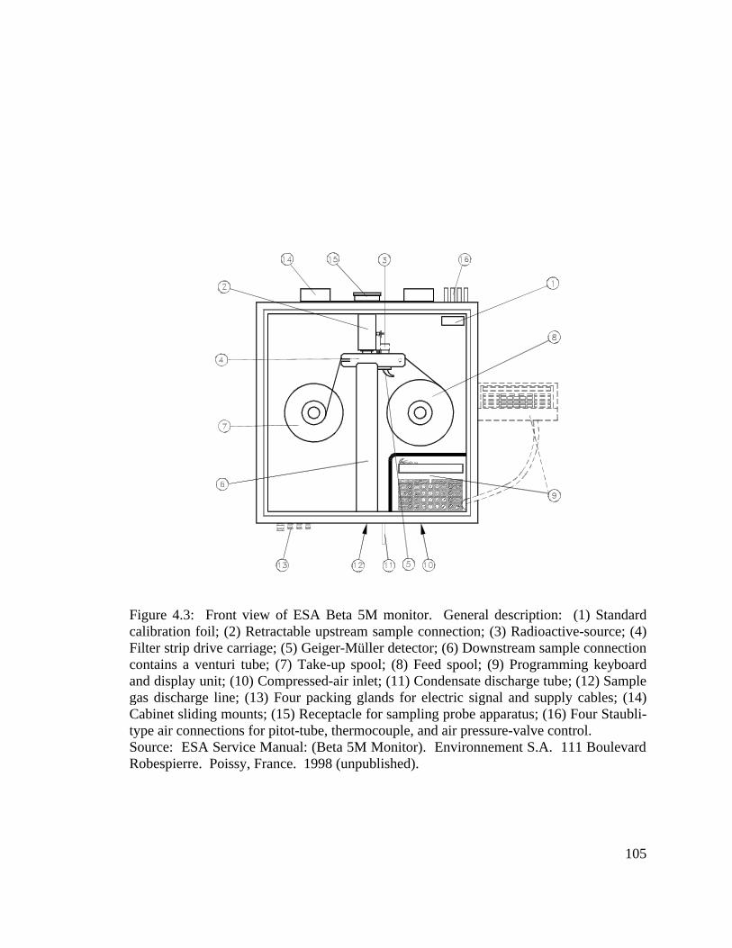
105
Figure 4.3: Front view of ESA Beta 5M monitor. General description: (1) Standard calibration foil; (2) Retractable upstream sample connection; (3) Radioactive-source; (4) Filter strip drive carriage; (5) Geiger-Müller detector; (6) Downstream sample connection contains a venturi tube; (7) Take-up spool; (8) Feed spool; (9) Programming keyboard and display unit; (10) Compressed-air inlet; (11) Condensate discharge tube; (12) Sample gas discharge line; (13) Four packing glands for electric signal and supply cables; (14) Cabinet sliding mounts; (15) Receptacle for sampling probe apparatus; (16) Four Staubli-type air connections for pitot-tube, thermocouple, and air pressure-valve control. Source: ESA Service Manual: (Beta 5M Monitor). Environnement S.A. 111 Boulevard Robespierre. Poissy, France. 1998 (unpublished).

106
Figure 4.4: Presentation of ESA monitor and probe assemble. Source: ESA Service Manual: (Beta 5M Monitor). Environnement S.A. 111 Boulevard Robespierre. Poissy, France. 1998 (unpublished).

107
b ca d
e
Figure 4.5: Diagram of side view of Sigrist CTNR Light-scattering monitor. General description: (a) Control unit; (b) Photometer; (c) Ring pipe and heated sampling line; (d) Gas duct or stack; (e) Fan blower. Source: Sigrist Service/Instruction Manuals. CTNR Light-scattering Monitor. Sigrist-Photometer AG. 1 Hofurlistrasse. Ennetburgen, Switzerland. 1998 (unpublished).

108
(a)
FF VF
L1L2
S1
P1
S2 S2
M
P2
(b)
Figure 4.6: Schematics of Sigrist photometer cell and optical sampling configuration. (a) Photometer cell: (P1) Sample entry point; (P2) Purge air and sample outlet; (S1) Purge air supply; (S2) Treated purge air; (L1) Light entry point; (L2) Light outlet at 15o; (M) Measurement point; (FF) Fine filter; (VF) Roughing Filter. (b) Optical sampling configuation: (B) Light from incandescent bulb; (Hn) Semi-transparent mirrors; (SM) Measuring beam; (SV) Reference beam; (P) Sample cell; (SL) 15o Scattered light; (F) detector; (R) Optical attenuator; (C) Chopper wheel and (M) motor; (E) Milliamp signal. Source: Sigrist Service/Instruction Manuals. CTNR Light-scattering Monitor. Sigrist-Photometer AG. 1 Hofurlistrasse. Ennetburgen, Switzerland. 1998 (unpublished).
B
P
RSV
SM
C F EH1 H2
MSL

109
Figure 5.1: Diagram of TSCA Incinerator stack sampling platforms and port elevations. (Adapted from: EERC, 1999).

110
Figure 5.2: Detail of TSCA Incinerator stack sampling ports. (Adapted from: EERC, 1999)

111
Figure 5.3: Reference Method 5i sampling train and filter holder assembly. Source: EPA (U.S. Environmental Protection Agency), "Method 5i: Determination of Low Level Particulate Matter Emissions from Stationary Sources", CFR 40 Part 60, Appendix A. Washington DC: July 1, 2000.

112
Figure 5.4: Layout of CEMS around incinerator stack. (Adapted from: EERC, 1999)

Figure 5.5: Schematic representing batch sampling cycle time of the beta-gauge monitors. Note: the total measuring cycle and actual sampling times are based upon a hypothetical reference method run. 113

Figure 6.1: Phase 2 M5i Cross Correlation (7 Runs Meeting RSD Criteria).
y = 0.954x + 0.3547R2 = 0.9768
-2
0
2
4
6
8
10
12
14
16
-2 0 2 4 6 8 10 12 14 16
Train-2 (mg/dscm @ 7% O2)
Tra
in-1
(m
g/d
scm
@ 7
% O
2)
Source Data
Best-fit Line
114

Figure 6.2: Phase 3 M5i Cross Correlation (19 Runs Meeting RSD Criteria).
y = 0.934x + 1.2611R2 = 0.9891
0
10
20
30
40
50
60
70
80
90
0 10 20 30 40 50 60 70 80 90
Train-2 (mg/dscm @ 7% O2)
Tra
in-1
(m
g/d
scm
@ 7
% O
2)
Source Data
Best-fit Line
115

Figure 6.3: Durag Linear Calibration Curve for Phase 3.
y = 9.5477x - 36.419
0
10
20
30
40
50
60
70
80
4.0 5.0 6.0 7.0 8.0 9.0 10.0 11.0 12.0
Durag (mA)
Met
ho
d 5
i (m
g/d
scm
-Du
rag
)
DataCI-upperCI-lowerTI-upperTI-lower125% LimitBest-fit
Emission Standardat Conditions of CEMS
CEMS Responseat Emission Standard
116

Figure 6.4: Durag Logarithmic Calibration Curve for Phase 3.
y = 59.899Ln(x) - 85.101
0
10
20
30
40
50
60
70
1.0 10.0 100.0
Durag (mA)
Met
ho
d 5
i (m
g/d
scm
-Du
rag
)
DataCI-upperCI-lowerTI-upperTI-lower125% LimitBest-fit
CEMS Responseat Emission Standard
Emission Standardat Condition of CEMS
117

Figure 6.5: Durag Polynomial Calibration Curve for Phase 3.
y = 0.2x2 + 6.8812x - 27.936
0
10
20
30
40
50
60
70
80
4.0 5.0 6.0 7.0 8.0 9.0 10.0 11.0 12.0Durag (mA)
Met
ho
d 5
i (m
g/d
scm
-Du
rag
)
DataCI-upperCI-lowerIT-upperTI-lower125% LimitBest-fit
Emission Standardat Condition of CEMS
CEMS Response at Emission Standard
118

Figure 6.6: ESA Linear Calibration Curve for Phase 3.
y = 1.105x + 1.2764
0
5
10
15
20
25
30
35
40
45
50
0 5 10 15 20 25 30 35 40 45 50
ESA (mg/Nm3)
Met
ho
d 5
i (m
g/N
m3 -E
SA
)
DataCI-upperCI-lowerTI-upperTI-lower125% LimitBest-fit
Emission Standardat Condition of CEMS
CEMS Responseat Emission Standard
119

Figure 6.7: ESA Logarithmic Calibration Curve for Phase 3.
y = 4.3592Ln(x) + 4.8684
-30
-20
-10
0
10
20
30
40
50
60
70
0.1 1.0 10.0 100.0
ESA (mg/Nm3)
Met
ho
d 5
i (m
g/N
m3 -E
SA
)
DataCI-upperCI-lowerTI-upperTI-lower125% LimitBest-fit
CEMS Responseat Emission Standard
Emission Standardat Condition of CEMS
120

Figure 6.8: ESA Polynomial Calibration Curve for Phase 3.
y = -0.0028x2 + 1.1812x + 0.9033
0
5
10
15
20
25
30
35
40
45
50
0 5 10 15 20 25 30 35 40 45 50ESA (mg/Nm3)
Met
ho
d 5
i (m
g/N
m3 -E
SA
)
DataCI-upperCI-lowerIT-upperTI-lower125% LimitBest-fit
Emission Standardat Condition of CEMS
CEMS Responseat Emission Standard
121

Figure 6.9: Sigrist Linear Calibration Curve for Phase 3.
y = 5.564x + 5.679
0
5
10
15
20
25
30
35
40
0.0 1.0 2.0 3.0 4.0 5.0
Sigrist (mg/m3 PLA)
Met
ho
d 5
i (m
g/m
3 -Sig
rist
)DataCI-upperCI-lowerTI-upperTI-lower125% LimitBest-fit
Emission Standardat Condition of CEMS
CEMS Responseat Emission Standard
122

Figure 6.10: Sigrist Logarithmic Calibration Curve for Phase 3.
y = 3.1848Ln(x) + 12.965
0
5
10
15
20
25
0.01 0.10 1.00 10.00
Sigrist (mg/m3 PLA)
Met
ho
d 5
i (m
g/m
3 -Sig
rist
)
DataCI-upperCI-lowerTI-upperTI-lower125% LimitBest-fit
Emission Standardat Condition of CEMS
CEMS Responseat Emission Standard
123

Figure 6.11: Sigrist Polynomial Calibration Curve for Phase 3.
y = -2.7715x2 + 14.243x + 3.3666
0
5
10
15
20
25
30
0.0 1.0 2.0 3.0 4.0 5.0
Sigrist (mg/m3 PLA)
Met
ho
d 5
i (m
g/m
3 -Sig
rist
)DataCI-upperCI-lowerTI-upperTI-lower125% LimitBest-fit
Emission Standardat Condition of CEMS
CEMS Responseat Emission Standard
124

Figure 6.12: ESA Phase 3 Linear Calibration Curve with Phase 2 Data Inserted for RCA.
0
5
10
15
20
25
30
35
40
45
50
0 5 10 15 20 25 30 35 40 45 50
ESA (mg/Nm3)
Met
ho
d 5
i (m
g/N
m3 -E
SA
) Phase 2
CI-upper
CI-lower
TI-upper
TI-lower
Best-fit
Emission Standardat Condition of CEMS
CEMS Responseat Emission Standard
125

Figure 6.13: Sigrist Phase 3 Logarithmic Calibration Curve with Phase 2 Data Inserted for RCA
0
5
10
15
20
25
0.001 0.010 0.100 1.000 10.000
Sigrist (mg/m3 PLA)
Met
ho
d 5
i (m
g/m
3 -Sig
rist
)
Phase 2
CI-upper
CI-lower
TI-upper
TI-lower
Best-fit
Emission Standardat Condition of CEMS
CEMS Responseat Emission Standard
126

Figure 6.14: Durag vs. ESA (1-hour Averages for October 19-22 & 24).
y = 0.6419x + 1.0902R2 = 0.9171
0
5
10
15
20
25
0 5 10 15 20 25 30
ESA (mg/Nm3)
Du
rag
(m
g/N
m3 )
127

Figure 6.15: Durag vs. Sigrist (1-hour Averages for October 19-22 & 24).
y = 5.2618x + 2.5319R2 = 0.7072
y = 2.4649Ln(x) + 10.543R2 = 0.8186
0
5
10
15
20
25
30
0.0 0.5 1.0 1.5 2.0 2.5 3.0 3.5 4.0 4.5 5.0
Sigrist (mg/Nm3 PLA)
Du
rag
(m
g/N
m3 )
128

Figure 6.16: ESA vs. Sigrist (1-hour Averages for October 19-22 & 24).
y = 7.4973x + 2.4914R2 = 0.6451
y = 3.8035Ln(x) + 14.635R2 = 0.8757
0
5
10
15
20
25
30
35
40
0.0 0.5 1.0 1.5 2.0 2.5 3.0 3.5 4.0 4.5 5.0
Sigrist (mg/Nm3 PLA)
ES
A (
mg
/Nm
3 )
129

Figure 6.17: Durag and ESA Responses vs. Waste Feeds During October 19.
0.0
10.0
20.0
30.0
40.0
0:00 4:00 8:00 12:00 16:00 20:00 0:00
Clock Time (24 hours)
CE
MS
(m
g/N
m3 )
-500
-400
-300
-200
-100
0
100
200
300
400
500
Was
te F
eed
(lb
s/h
r)
Durag ESA IWS-1 IWS-2 Primary Aqueous Secondary
130

Figure 6.18: Sigrist Response vs. Waste Feeds During October 19.
0.0
5.0
10.0
15.0
20.0
25.0
30.0
0:00 4:00 8:00 12:00 16:00 20:00 0:00
Clock Time (24 hours)
CE
MS
(m
g/m
3 PL
A)
-500
-400
-300
-200
-100
0
100
200
300
400
500
Was
te F
eed
(lb
s/h
r)
Sigrist IWS-1 IWS-2 Primary Aqueous Secondary
131

132
Appendix C
Airtech Laboratory Report Phase 3 M5i Testing

133
Appendix C: Runs R26-R27Phase 3: Modified from Airtech Final Laboratory Report December 15, 2000
Test Parameters R26-T1 R26-T2 R27-T1 R27-T2Date 10/19/2000 10/19/2000 10/19/2000 10/19/2000First Port Start Time 8:19 8:19 10:59 10:59First Port Stop Time 8:49 8:49 11:29 11:29
Second Port Start Time 9:01 9:01 11:49 11:49Second Port Stop Time 9:42 9:42 12:20 12:20
Filter Observations No Change No Change No Change No ChangeTesting Anomalies Noted Delay5 Delay5 None None
Gas ConditionsTemperature (oF) 177 180 176 179Volumetric Flow Rate (acfm) 19,100 19,800 18,500 18,900Volumetric Flow Rate (scfm) 15,600 16,100 15,100 15,300Volumetric Flow Rate (dscfm) 8,390 8,090 8,000 8,130Carbon Dioxide (%) 6.8 6.6 6.4 6.6Oxygen (%) 10.80 10.80 11.00 10.80Moisture (%) 46.21 49.73 47.17 46.96
Particulate ResultsParticulate Concentration (grains/dscf @ 7% O2) 0.00998 0.00972 0.0141 0.0145Particulate Concentration (mg/dscm @ 7% O2) 22.8 22.3 32.4 33.3
Particulate Concentration (mg/acm) 7.28 6.60 9.95 10.4Particulate Concentration (mg/dNcm-Durag)1 16.59 16.17 23.05 24.17Particulate Concentration (mg/Ncm-ESA)2 9.580 8.722 13.07 13.76Particulate Concentration (mg/cm-Sigrist)3 6.041 5.500 8.242 8.676
Particulate Concentration (mg/Ncm-ESA) act moist2,4 NA NA 12.8 NAParticulate Concentration (mg/cm-Sigrist) act moist3,4 NA NA 8.10 NA
Particulate Emission Rate (lb/hr) 0.521 0.490 0.690 0.736Particulate Emission Rate (lb/day) 12.5 11.8 16.6 17.7
1 - Units expressed as mg/dNcm-Durag are reported dry and are corrected to 20oC and 1013 mbar.2 - Units expressed as mg/Ncm-ESA are reported wet and are corrected to 0oC and 1013 mbar.3 - Units expressed as mg/cm-Sigrist are reported wet and are corrected to 160oC and 1013 mbar.4 - Units reported as "act moist" disregard the moisture saturation point. Measured moisture values were used for all calcs. NA indicates that the measured value did not exceed saturation.
5 - Run 26: Stop at 9:14, Re-start 9:24. Change sample train component.
AveragesDurag
ESASigrist
OxygenMoisture
Stack Temperature
Particulate Concentration (mg/dscm @ 7% O2) 22.8 22.3 32.4 33.3
16.389.1515.77110.8047.97178.4
R26 (T1&T2) R27 (T1&T2)23.6113.418.45910.9047.07177.5

134
Appendix C: Runs R28-R29Phase 3: continued AES Report December 15, 2000
Test Parameters R28-T1 R28-T2 R29-T1 R29-T2Date 10/19/2000 10/19/2000 10/19/2000 10/19/2000First Port Start Time 14:43 14:43 16:34 16:34First Port Stop Time 15:13 15:13 17:33 17:33
Second Port Start Time 15:21 15:21 17:44 17:44Second Port Stop Time 15:51 15:51 18:23 18:23
Filter Observations No Change No Change No Change No ChangeTesting Anomalies Noted None None Filter6 Filter6
Gas ConditionsTemperature (oF) 176 179 177 178Volumetric Flow Rate (acfm) 18,600 19,800 17,500 18,800Volumetric Flow Rate (scfm) 15,200 16,100 14,300 15,300Volumetric Flow Rate (dscfm) 7,990 7,940 7,370 7,810Carbon Dioxide (%) 6.6 6.4 6.6 6.8Oxygen (%) 10.00 10.40 10.20 10.20Moisture (%) 47.51 50.63 48.42 49.15
Particulate ResultsParticulate Concentration (grains/dscf @ 7% O2) 0.0103 0.0118 0.0226 0.0222Particulate Concentration (mg/dscm @ 7% O2) 23.5 27.1 51.7 50.9
Particulate Concentration (mg/acm) 7.90 8.21 16.8 16.2Particulate Concentration (mg/dNcm-Durag)1 18.44 20.45 39.82 39.14Particulate Concentration (mg/Ncm-ESA)2 10.38 10.84 22.04 21.36Particulate Concentration (mg/cm-Sigrist)3 6.548 6.835 13.90 13.47
Particulate Concentration (mg/Ncm-ESA) act moist2,4 NA NA 22.0 20.8Particulate Concentration (mg/cm-Sigrist) act moist3,4 NA NA 13.9 13.1
Particulate Emission Rate (lb/hr) 0.552 0.608 1.10 1.14Particulate Emission Rate (lb/day) 13.2 14.6 26.4 27.5
1 - Units expressed as mg/dNcm-Durag are reported dry and are corrected to 20oC and 1013 mbar.2 - Units expressed as mg/Ncm-ESA are reported wet and are corrected to 0oC and 1013 mbar.3 - Units expressed as mg/cm-Sigrist are reported wet and are corrected to 160oC and 1013 mbar.4 - Units reported as "act moist" disregard the moisture saturation point. Measured moisture values were used for all calcs. NA indicates that the measured value did not exceed saturation.
6 - Run 29: Stop in first port at 16:58. Re-start 17:28. Stop in second port at 17:52. Re-start 18:00. Both stops to change out filter.
AveragesDurag
ESASigrist
OxygenMoisture
Stack Temperature
Particulate Concentration (mg/dscm @ 7% O2) 23.5 27.1 51.7 50.9
177.7 177.2
10.20 10.2049.07 48.79
10.61 21.706.692 13.69
R28 (T1&T2) R29 (T1&T2)19.44 39.48

135
Appendix C: Runs R30-R31Phase 3: continued AES Report December 15, 2000
Test Parameters R30-T1 R30-T2 R31-T1 R31-T2Date 10/19/2000 10/19/2000 10/20/2000 10/20/2000First Port Start Time 19:04 19:04 8:55 8:55First Port Stop Time 19:34 19:34 9:25 9:25
Second Port Start Time 19:41 19:41 9:30 9:30Second Port Stop Time 20:36 20:36 10:00 10:00
Filter Observations No Change No Change No Change No ChangeTesting Anomalies Noted Filter7 None None None
Gas ConditionsTemperature (oF) 177 179 177 180Volumetric Flow Rate (acfm) 18,500 18,700 18,600 18,500Volumetric Flow Rate (scfm) 15,100 15,200 15,100 15,000Volumetric Flow Rate (dscfm) 7,820 7,600 8,320 7,720Carbon Dioxide (%) 6.8 6.8 6.4 6.8Oxygen (%) 10.00 10.00 9.90 9.60Moisture (%) 48.09 50.03 45.00 48.44
Particulate ResultsParticulate Concentration (grains/dscf @ 7% O2) 0.0350 0.0335 0.02391 0.02109Particulate Concentration (mg/dscm @ 7% O2) 80.0 76.6 54.7 48.3
Particulate Concentration (mg/acm) 26.6 24.4 19.4 16.4Particulate Concentration (mg/dNcm-Durag)1 62.75 60.08 43.30 39.22Particulate Concentration (mg/Ncm-ESA)2 34.96 32.22 25.56 21.71Particulate Concentration (mg/cm-Sigrist)3 22.05 20.32 16.12 13.69
Particulate Concentration (mg/Ncm-ESA) act moist2,4 NA NA NA NAParticulate Concentration (mg/cm-Sigrist) act moist3,4 NA NA NA NA
Particulate Emission Rate (lb/hr) 1.84 1.71 1.35 1.14Particulate Emission Rate (lb/day) 44.1 41.1 32.4 27.2
1 - Units expressed as mg/dNcm-Durag are reported dry and are corrected to 20oC and 1013 mbar.2 - Units expressed as mg/Ncm-ESA are reported wet and are corrected to 0oC and 1013 mbar.3 - Units expressed as mg/cm-Sigrist are reported wet and are corrected to 160oC and 1013 mbar.4 - Units reported as "act moist" disregard the moisture saturation point. Measured moisture values were used for all calcs. NA indicates that the measured value did not exceed saturation.
5 - Filters in both sample trains were changed between ports.7 - Run 30 T 1: Filter changed during port change. Stop Run 19:52, Restart 20:17
AveragesDurag
ESASigrist
OxygenMoisture
Stack Temperature
Particulate Concentration (mg/dscm @ 7% O2) 80.0 76.6 54.7 48.3
R31 (T1&T2)41.26
178.5
9.7546.72
23.6314.90
178.1
10.0049.06
R30 (T1&T2)61.4233.5921.18
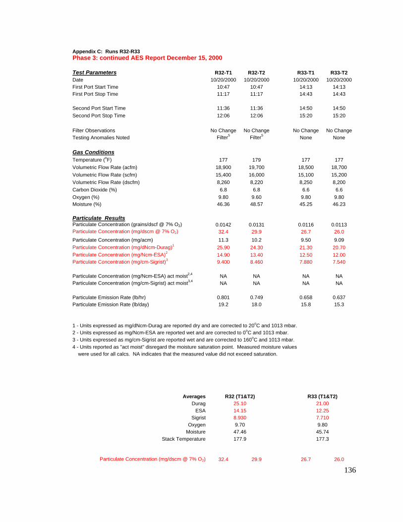
136
Appendix C: Runs R32-R33Phase 3: continued AES Report December 15, 2000
Test Parameters R32-T1 R32-T2 R33-T1 R33-T2Date 10/20/2000 10/20/2000 10/20/2000 10/20/2000First Port Start Time 10:47 10:47 14:13 14:13First Port Stop Time 11:17 11:17 14:43 14:43
Second Port Start Time 11:36 11:36 14:50 14:50Second Port Stop Time 12:06 12:06 15:20 15:20
Filter Observations No Change No Change No Change No ChangeTesting Anomalies Noted Filter5 Filter5 None None
Gas ConditionsTemperature (oF) 177 179 177 177Volumetric Flow Rate (acfm) 18,900 19,700 18,500 18,700Volumetric Flow Rate (scfm) 15,400 16,000 15,100 15,200Volumetric Flow Rate (dscfm) 8,260 8,220 8,250 8,200Carbon Dioxide (%) 6.8 6.8 6.6 6.6Oxygen (%) 9.80 9.60 9.80 9.80Moisture (%) 46.36 48.57 45.25 46.23
Particulate ResultsParticulate Concentration (grains/dscf @ 7% O2) 0.0142 0.0131 0.0116 0.0113Particulate Concentration (mg/dscm @ 7% O2) 32.4 29.9 26.7 26.0
Particulate Concentration (mg/acm) 11.3 10.2 9.50 9.09Particulate Concentration (mg/dNcm-Durag)1 25.90 24.30 21.30 20.70Particulate Concentration (mg/Ncm-ESA)2 14.90 13.40 12.50 12.00Particulate Concentration (mg/cm-Sigrist)3 9.400 8.460 7.880 7.540
Particulate Concentration (mg/Ncm-ESA) act moist2,4 NA NA NA NAParticulate Concentration (mg/cm-Sigrist) act moist3,4 NA NA NA NA
Particulate Emission Rate (lb/hr) 0.801 0.749 0.658 0.637Particulate Emission Rate (lb/day) 19.2 18.0 15.8 15.3
1 - Units expressed as mg/dNcm-Durag are reported dry and are corrected to 20oC and 1013 mbar.2 - Units expressed as mg/Ncm-ESA are reported wet and are corrected to 0oC and 1013 mbar.3 - Units expressed as mg/cm-Sigrist are reported wet and are corrected to 160oC and 1013 mbar.4 - Units reported as "act moist" disregard the moisture saturation point. Measured moisture values were used for all calcs. NA indicates that the measured value did not exceed saturation.
AveragesDurag
ESASigrist
OxygenMoisture
Stack Temperature
Particulate Concentration (mg/dscm @ 7% O2) 32.4 29.9 26.7 26.0
9.7047.46177.9
R33 (T1&T2)21.0012.257.710
177.3
9.8045.74
R32 (T1&T2)25.1014.158.930

137
Appendix C: Runs R34-R35Phase 3: continued AES Report December 15, 2000
Test Parameters R34-T1 R34-T2 R35-T1 R35-T2Date 10/20/2000 10/20/2000 10/20/2000 10/20/2000First Port Start Time 15:56 15:56 17:33 17:33First Port Stop Time 16:26 16:26 18:03 18:03
Second Port Start Time 16:32 16:32 18:16 18:16Second Port Stop Time 17:02 17:02 18:46 18:46
Filter Observations No Change No Change No Change No ChangeTesting Anomalies Noted None None None None
Gas ConditionsTemperature (oF) 177 178 178 178Volumetric Flow Rate (acfm) 19,200 18,700 19,600 19,400Volumetric Flow Rate (scfm) 15,700 15,300 16,000 15,800Volumetric Flow Rate (dscfm) 8,410 8,180 8,360 8,490Carbon Dioxide (%) 6.8 6.8 6.8 6.6Oxygen (%) 9.60 9.70 9.80 10.00Moisture (%) 46.40 46.58 47.65 46.15
Particulate ResultsParticulate Concentration (grains/dscf @ 7% O2) 0.0107 0.0119 0.0170 0.0165Particulate Concentration (mg/dscm @ 7% O2) 24.5 27.2 38.9 37.8
Particulate Concentration (mg/acm) 8.69 9.53 13.3 13.0Particulate Concentration (mg/dNcm-Durag)1 19.88 21.90 31.07 29.64Particulate Concentration (mg/Ncm-ESA)2 11.44 12.55 17.45 17.13Particulate Concentration (mg/cm-Sigrist)3 7.213 7.916 11.01 10.80
Particulate Concentration (mg/Ncm-ESA) act moist2,4 NA NA NA NAParticulate Concentration (mg/cm-Sigrist) act moist3,4 NA NA NA NA
Particulate Emission Rate (lb/hr) 0.627 0.671 0.973 0.943Particulate Emission Rate (lb/day) 15.0 16.0 23.3 22.6
1 - Units expressed as mg/dNcm-Durag are reported dry and are corrected to 20oC and 1013 mbar.2 - Units expressed as mg/Ncm-ESA are reported wet and are corrected to 0oC and 1013 mbar.3 - Units expressed as mg/cm-Sigrist are reported wet and are corrected to 160oC and 1013 mbar.4 - Units reported as "act moist" disregard the moisture saturation point. Measured moisture values were used for all calcs. NA indicates that the measured value did not exceed saturation.
AveragesDurag
ESASigrist
OxygenMoisture
Stack Temperature
Particulate Concentration (mg/dscm @ 7% O2) 24.5 27.2 38.9 37.8
R34 (T1&T2)20.8912.007.564
R35 (T1&T2)30.3517.2910.90
177.6
9.9046.90
177.5
9.6546.49

138
Appendix C: Runs R36-R37Phase 3: continued AES Report December 15, 2000
Test Parameters R36-T1 R36-T2 R37-T1 R37-T2Date 10/21/2000 10/21/2000 10/21/2000 10/21/2000First Port Start Time 9:00 9:00 10:40 10:40First Port Stop Time 9:30 9:30 11:10 11:10
Second Port Start Time 9:37 9:37 11:16 11:16Second Port Stop Time 10:07 10:07 11:46 11:46
Filter Observations No Change No Change Black BlackTesting Anomalies Noted None None None None
Gas ConditionsTemperature (oF) 177 180 178 180Volumetric Flow Rate (acfm) 18,100 18,300 18,200 18,000Volumetric Flow Rate (scfm) 14,700 14,800 14,800 14,600Volumetric Flow Rate (dscfm) 7,790 7,990 7,760 7,740Carbon Dioxide (%) 5.8 6.0 6.8 6.8Oxygen (%) 10.80 10.60 9.80 9.95Moisture (%) 47.22 46.19 47.74 47.06
Particulate ResultsParticulate Concentration (grains/dscf @ 7% O2) 0.00242 0.00228 0.00378 0.00361Particulate Concentration (mg/dscm @ 7% O2) 5.55 5.21 8.65 8.26
Particulate Concentration (mg/acm) 1.74 1.69 2.95 2.80Particulate Concentration (mg/dNcm-Durag)1 4.030 3.860 6.905 6.510Particulate Concentration (mg/Ncm-ESA)2 2.282 2.229 3.873 3.699Particulate Concentration (mg/cm-Sigrist)3 1.439 1.406 2.442 2.332
Particulate Concentration (mg/Ncm-ESA) act moist2,4 NA NA NA NAParticulate Concentration (mg/cm-Sigrist) act moist3,4 NA NA NA NA
Particulate Emission Rate (lb/hr) 0.118 0.115 0.201 0.189Particulate Emission Rate (lb/day) 2.82 2.77 4.82 4.53
1 - Units expressed as mg/dNcm-Durag are reported dry and are corrected to 20oC and 1013 mbar.2 - Units expressed as mg/Ncm-ESA are reported wet and are corrected to 0oC and 1013 mbar.3 - Units expressed as mg/cm-Sigrist are reported wet and are corrected to 160oC and 1013 mbar.4 - Units reported as "act moist" disregard the moisture saturation point. Measured moisture values were used for all calcs. NA indicates that the measured value did not exceed saturation.
AveragesDurag
ESASigrist
OxygenMoisture
Stack Temperature
Particulate Concentration (mg/dscm @ 7% O2) 5.55 5.21 8.65 8.26
R36 (T1&T2) R37 (T1&T2)3.945 6.7082.256 3.7861.423 2.387
178.6 179.0
10.70 9.8846.71 47.40

139
Appendix C: Runs R38-R39Phase 3: continued AES Report December 15, 2000
Test Parameters R38-T1 R38-T2 R39-T1 R39-T2Date 10/21/2000 10/21/2000 10/22/2000 10/22/2000First Port Start Time 12:14 12:14 8:04 8:04First Port Stop Time 12:44 12:44 8:34 8:34
Second Port Start Time 12:51 12:51 8:55 8:55Second Port Stop Time 13:21 13:21 9:25 9:25
Filter Observations Slight yellow/greenSlight yellow/green No Change No ChangeTesting Anomalies Noted None None None None
Gas ConditionsTemperature (oF) 179 180 178 179Volumetric Flow Rate (acfm) 17,800 18,700 17,800 18,100Volumetric Flow Rate (scfm) 14,500 15,200 14,500 14,700Volumetric Flow Rate (dscfm) 7,690 8,150 7,560 7,790Carbon Dioxide (%) 6.7 6.8 7.0 7.0Oxygen (%) 9.95 9.80 9.60 9.60Moisture (%) 47.14 46.48 47.99 47.18
Particulate ResultsParticulate Concentration (grains/dscf @ 7% O2) 0.00597 0.00590 0.0147 0.0144Particulate Concentration (mg/dscm @ 7% O2) 13.7 13.5 33.6 33.1
Particulate Concentration (mg/acm) 4.64 4.70 11.6 11.6Particulate Concentration (mg/dNcm-Durag)1 10.77 10.79 27.35 26.87Particulate Concentration (mg/Ncm-ESA)2 6.109 6.195 15.27 15.23Particulate Concentration (mg/cm-Sigrist)3 3.853 3.907 9.627 9.606
Particulate Concentration (mg/Ncm-ESA) act moist2,4 NA NA NA NAParticulate Concentration (mg/cm-Sigrist) act moist3,4 NA NA NA NA
Particulate Emission Rate (lb/hr) 0.310 0.329 0.774 0.784Particulate Emission Rate (lb/day) 7.44 7.90 18.6 18.8
1 - Units expressed as mg/dNcm-Durag are reported dry and are corrected to 20oC and 1013 mbar.2 - Units expressed as mg/Ncm-ESA are reported wet and are corrected to 0oC and 1013 mbar.3 - Units expressed as mg/cm-Sigrist are reported wet and are corrected to 160oC and 1013 mbar.4 - Units reported as "act moist" disregard the moisture saturation point. Measured moisture values were used for all calcs. NA indicates that the measured value did not exceed saturation.
AveragesDurag
ESASigrist
OxygenMoisture
Stack Temperature
Particulate Concentration (mg/dscm @ 7% O2) 13.7 13.5 33.6 33.1
R39 (T1&T2)27.11
178.7
9.6047.59
15.259.617
179.1
9.8846.81
R38 (T1&T2)10.786.1523.880

140
Appendix C: Runs R40-R41Phase 3: continued AES Report December 15, 2000
Test Parameters R40-T1 R40-T2 R41-T1 R41-T2Date 10/22/2000 10/22/2000 10/22/2000 10/22/2000First Port Start Time 10:30 10:30 12:08 12:08First Port Stop Time 11:00 11:00 12:38 12:38
Second Port Start Time 11:10 11:10 12:43 12:43Second Port Stop Time 11:40 11:40 13:13 13:13
Filter Observations No Change No Change No Change No ChangeTesting Anomalies Noted None None None None
Gas ConditionsTemperature (oF) 177 180 178 180Volumetric Flow Rate (acfm) 17,700 18,100 18,000 18,200Volumetric Flow Rate (scfm) 14,400 14,800 14,700 14,800Volumetric Flow Rate (dscfm) 7,480 7,640 7,570 7,720Carbon Dioxide (%) 6.9 7.0 6.9 7.0Oxygen (%) 9.90 9.80 9.95 9.80Moisture (%) 48.22 48.27 48.54 47.92
Particulate ResultsParticulate Concentration (grains/dscf @ 7% O2) 0.0179 0.0164 0.0139 0.0137Particulate Concentration (mg/dscm @ 7% O2) 41.0 37.6 31.8 31.4
Particulate Concentration (mg/acm) 13.7 12.7 10.5 10.6Particulate Concentration (mg/dNcm-Durag)1 32.42 30.00 25.07 25.07Particulate Concentration (mg/Ncm-ESA)2 18.02 16.70 13.85 14.01Particulate Concentration (mg/cm-Sigrist)3 11.36 10.50 8.732 8.837
Particulate Concentration (mg/Ncm-ESA) act moist2,4 NA NA NA NAParticulate Concentration (mg/cm-Sigrist) act moist3,4 NA NA NA NA
Particulate Emission Rate (lb/hr) 0.909 0.858 0.711 0.725Particulate Emission Rate (lb/day) 21.8 20.6 17.1 17.4
1 - Units expressed as mg/dNcm-Durag are reported dry and are corrected to 20oC and 1013 mbar.2 - Units expressed as mg/Ncm-ESA are reported wet and are corrected to 0oC and 1013 mbar.3 - Units expressed as mg/cm-Sigrist are reported wet and are corrected to 160oC and 1013 mbar.4 - Units reported as "act moist" disregard the moisture saturation point. Measured moisture values were used for all calcs. NA indicates that the measured value did not exceed saturation.
AveragesDurag
ESASigrist
OxygenMoisture
Stack Temperature
Particulate Concentration (mg/dscm @ 7% O2) 41.0 37.6 31.8 31.4
9.8548.24178.5
R41 (T1&T2)25.0713.938.785
179.2
9.8848.23
R40 (T1&T2)31.2117.3610.93

141
Appendix C: Runs R42-R43Phase 3: continued AES Report December 15, 2000
Test Parameters R42-T1 R42-T2 R43-T1 R43-T2Date 10/22/2000 10/22/2000 10/22/2000 10/22/2000First Port Start Time 14:28 14:28 16:00 16:00First Port Stop Time 14:58 14:58 16:30 16:30
Second Port Start Time 15:03 15:03 16:34 16:34Second Port Stop Time 15:33 15:33 17:04 17:04
Filter Observations No Change No Change No Change No ChangeTesting Anomalies Noted None None None None
Gas ConditionsTemperature (oF) 179 180 179 180Volumetric Flow Rate (acfm) 17,900 18,900 18,800 18,700Volumetric Flow Rate (scfm) 14,600 15,400 15,300 15,200Volumetric Flow Rate (dscfm) 7,520 7,970 8,020 7,940Carbon Dioxide (%) 7.0 7.0 6.2 6.0Oxygen (%) 9.8 9.9 9.8 10.0Moisture (%) 48.6 48.2 47.6 47.9
Particulate ResultsParticulate Concentration (grains/dscf @ 7% O2) 0.0139 0.0139 0.0152 0.0146Particulate Concentration (mg/dscm @ 7% O2) 31.9 31.8 34.9 33.5
Particulate Concentration (mg/acm) 10.7 10.6 11.9 11.1Particulate Concentration (mg/dNcm-Durag)1 25.56 25.19 27.83 26.24Particulate Concentration (mg/Ncm-ESA)2 14.10 14.01 15.64 14.68Particulate Concentration (mg/cm-Sigrist)3 8.892 8.832 9.861 9.255
Particulate Concentration (mg/Ncm-ESA) act moist2,4 NA NA NA NAParticulate Concentration (mg/cm-Sigrist) act moist3,4 NA NA NA NA
Particulate Emission Rate (lb/hr) 0.720 0.752 0.836 0.781Particulate Emission Rate (lb/day) 17.3 18.1 20.1 18.7
1 - Units expressed as mg/dNcm-Durag are reported dry and are corrected to 20oC and 1013 mbar.2 - Units expressed as mg/Ncm-ESA are reported wet and are corrected to 0oC and 1013 mbar.3 - Units expressed as mg/cm-Sigrist are reported wet and are corrected to 160oC and 1013 mbar.4 - Units reported as "act moist" disregard the moisture saturation point. Measured moisture values were used for all calcs. NA indicates that the measured value did not exceed saturation.
AveragesDurag
ESASigrist
OxygenMoisture
Stack Temperature
Particulate Concentration (mg/dscm @ 7% O2) 31.9 31.8 34.9 33.5
R42 (T1&T2)25.3714.058.862
R43 (T1&T2)27.0415.169.558
179.2
9.9047.77
179.3
9.8348.39

142
Appendix C: Runs R44-R45Phase 3: continued AES Report December 15, 2000
Test Parameters R44-T1 R44-T2 R45-T1 R45-T2Date 10/24/2000 10/24/2000 10/24/2000 10/24/2000First Port Start Time 8:24 8:24 11:07 11:07First Port Stop Time 9:24 9:24 12:07 12:07
Second Port Start Time 9:34 9:34 12:15 12:15Second Port Stop Time 10:34 10:34 13:15 13:15
Filter Observations No Change No Change No Change No ChangeTesting Anomalies Noted None None None None
Gas ConditionsTemperature (oF) 178 180 177 179Volumetric Flow Rate (acfm) 17,800 17,500 17,700 18,000Volumetric Flow Rate (scfm) 14,600 14,300 14,600 14,800Volumetric Flow Rate (dscfm) 7,750 7,660 7,640 7,690Carbon Dioxide (%) 6.0 6.5 6.4 6.4Oxygen (%) 10.80 10.70 10.00 10.20Moisture (%) 46.86 46.52 47.50 47.95
Particulate ResultsParticulate Concentration (grains/dscf @ 7% O2) 0.000810 0.000775 0.000920 0.000545Particulate Concentration (mg/dscm @ 7% O2) 1.85 1.77 2.11 1.25
Particulate Concentration (mg/acm) 0.588 0.570 0.714 0.410Particulate Concentration (mg/dNcm-Durag)1 1.347 1.302 1.650 0.9599Particulate Concentration (mg/Ncm-ESA)2 0.7682 0.7473 0.9310 0.5363Particulate Concentration (mg/cm-Sigrist)3 0.4845 0.4713 0.5870 0.3382
Particulate Concentration (mg/Ncm-ESA) act moist2,4 NA NA NA NAParticulate Concentration (mg/cm-Sigrist) act moist3,4 NA NA NA NA
Particulate Emission Rate (lb/hr) 0.0391 0.0374 0.0474 0.0277Particulate Emission Rate (lb/day) 0.939 0.897 1.14 0.664
1 - Units expressed as mg/dNcm-Durag are reported dry and are corrected to 20oC and 1013 mbar.2 - Units expressed as mg/Ncm-ESA are reported wet and are corrected to 0oC and 1013 mbar.3 - Units expressed as mg/cm-Sigrist are reported wet and are corrected to 160oC and 1013 mbar.4 - Units reported as "act moist" disregard the moisture saturation point. Measured moisture values were used for all calcs. NA indicates that the measured value did not exceed saturation.
AveragesDurag
ESASigrist
OxygenMoisture
Stack Temperature
Particulate Concentration (mg/dscm @ 7% O2) 1.85 1.77 2.11 1.25
R44 (T1&T2) R45 (T1&T2)1.325 1.3050.7578 0.73360.4779 0.4626
178.8 178.0
10.8 10.146.69 47.72

143
Appendix D
Summary of M5i and CEMS Data for Phase 3 Testing

144
Appendix D: Summary of M5i and CEMS Data for Phase 3 Testing.
(continued)
Phase 3 ***** DateReference Method 5i - Time R26 R27 R28 R29 R30 R31 R32 R33 R34 R35
Start Time 8:19 10:59 14:43 16:34 19:04 8:55 10:47 14:13 15:56 17:33
Port Stop 1 8:49 11:29 15:13 16:58 19:34 9:25 11:17 14:43 16:26 18:03
Port Start 1 9:01 11:49 15:21 17:28 19:41 9:30 11:36 14:50 16:32 18:16
Port Stop 2 9:14 - - 17:33 19:52 - - - - -
Port Start 2 9:24 - - 17:44 20:17 - - - - -
Port Stop 3 - - 17:52 - - - - -
Port Start 3 - - - 18:00 - - - - -
Stop Time 9:42 12:20 15:51 18:23 20:36 10:00 12:06 15:20 17:02 18:46
Total = 1:01 1:01 1:00 1:00 1:00 1:00 1:00 1:00 1:00 1:00
Reference Method 5i - Data R26 R27 R28 R29 R30 R31 R32 R33 R34 R35
Average Durag (mg/dscm) 16.38 23.61 19.44 39.48 61.42 41.26 25.10 21.00 20.89 30.35Average ESA (mg/Nm3) 9.151 13.41 10.61 21.70 33.59 23.63 14.15 12.25 12.00 17.29
Average Sigrist (mg/m3 PLA) 5.771 8.459 6.692 13.69 21.18 14.90 8.930 7.710 7.564 10.90
Average Oxygen Percent 10.8 10.9 10.2 10.2 10.0 9.75 9.70 9.80 9.65 9.90
Average Moisture Percent 47.97 47.07 49.07 48.79 49.06 46.72 47.46 45.74 46.49 46.90Average Stack Temperature (oF) 178.4 177.5 177.7 177.2 178.1 178.5 177.9 177.3 177.5 177.6
Average Abs Stack Press (in Hg) 29.44 29.44 29.44 29.44 29.44 29.44 29.44 29.44 29.44 29.44
Incinerator Data R26 R27 R28 R29 R30 R31 R32 R33 R34 R35
Average Sigrist (mg/m3 PLA) 0.253909 0.511662 0.239761 1.425907 3.218443 0.529626 0.343226 0.228386 0.367018 0.544798
Average Durag (mA) @ dscm 5.581 6.583 5.891 8.654 9.457 8.433 6.579 5.834 5.848 6.894Average ESA (mg/Nm3) 8.67 10.30 9.21 19.69 29.21 20.95 12.50 10.55 10.31 10.86
Average Stack Pressure (mm Hg) 758.08 758.58 757.74 758.24 757.10 758.37 758.62 758.37 758.01 758.03Average Stack Temperature (oF) 177.3 177.2 178.2 178.1 177.2 178.3 177.5 178.5 178.6 178.6
Average Oxygen Percent 10.4 10.2 10.1 9.9 10.1 10.0 10.1 10.0 9.9 9.9
Ave Primary Waste Feed Rate (lb/hr) 263.3 269.6 259.5 311.0 339.4 0.0 288.3 285.4 286.9 286.4
Ave Aqueous Waste Feed Rate (lb/hr) 176.5 176.6 176.4 255.4 306.5 305.9 180.9 183.3 183.3 256.7
Ave Secondary Waste Feed Rate (lb/hr) 259.0 259.4 259.0 313.3 351.9 0.0 284.2 309.5 309.4 308.9
Ave Solid Waste Feed Rate (lb/hr) 0.0 0.0 0.0 0.0 0.0 0.0 112.2 127.5 152.6 163.2
Ave Saturation Pressure (mm Hg) 366.14 365.38 373.92 372.60 365.22 374.50 367.63 376.21 376.69 376.90
Average Moisture Percent 48.30 48.17 49.35 49.14 48.24 49.38 48.46 49.61 49.69 49.72
19-Oct 20-Oct
Phase 3 ***** Date
Reference Method 5i - Time R36 R37 R38 R39 R40 R41 R42 R43 R44 R45
Start Time 9:00 10:40 12:14 8:04 10:30 12:08 14:28 16:00 8:24 11:07
Port Stop 1 9:30 11:10 12:44 8:34 11:00 12:38 14:58 16:30 9:24 12:07
Port Start 1 9:37 11:16 12:51 8:55 11:10 12:43 15:03 16:34 9:34 12:15
Port Stop 2 - - - - - - - - - -
Port Start 2 - - - - - - - - - -
Port Stop 3 - - - - - - - - - -
Port Start 3 - - - - - - - - - -
Stop Time 10:07 11:46 13:21 9:25 11:40 13:13 15:33 17:04 10:34 13:15
Total = 1:00 1:00 1:00 1:00 1:00 1:00 1:00 1:00 2:00 2:00
Reference Method 5i - Data R36 R37 R38 R39 R40 R41 R42 R43 R44 R45
Average Durag (mg/dscm) 3.945 6.708 10.78 27.11 31.21 25.07 25.37 27.04 1.325 1.305Average ESA (mg/Nm3) 2.256 3.786 6.152 15.25 17.36 13.93 14.05 15.16 0.7578 0.7336
Average Sigrist (mg/m3 PLA) 1.423 2.387 3.880 9.617 10.93 8.785 8.862 9.558 0.4779 0.4626
Average Oxygen Percent 10.7 9.88 9.88 9.60 9.85 9.88 9.83 9.90 10.75 10.1
Average Moisture Percent 46.71 47.40 46.81 47.59 48.24 48.23 48.39 47.77 46.69 47.72Average Stack Temperature (oF) 178.6 179.0 179.1 178.7 178.5 179.2 179.3 179.2 178.8 178.0
Average Abs Stack Press (in Hg) 29.49 29.49 29.49 29.54 29.54 29.54 29.54 29.54 29.69 29.69
Incinerator Data R36 R37 R38 R39 R40 R41 R42 R43 R44 R45
Average Sigrist (mg/m3 PLA) 0.011863 0.054513 0.031211 0.383198 0.599869 0.286351 0.320300 0.305484 0.018696 0.017807
Average Durag (mA) @ dscm 4.305 4.525 4.415 6.616 6.373 6.353 6.659 6.916 4.475 4.421Average ESA (mg/Nm3) 0.55 3.13 4.52 12.58 12.99 10.75 11.36 11.96 0.08 0.14
Average Stack Pressure (mm Hg) 758.70 759.81 760.08 761.75 762.90 763.66 764.61 764.85 763.89 764.29Average Stack Temperature (oF) 178.5 179.1 179.4 179.1 179.1 179.7 180.1 179.7 178.4 178.9
Average Oxygen Percent 10.2 9.9 10.0 9.8 9.8 9.8 9.6 9.8 10.2 10.1
Ave Primary Waste Feed Rate (lb/hr) 64.3 189.7 243.1 141.4 237.2 260.9 258.7 258.4 261.7 256.6
Ave Aqueous Waste Feed Rate (lb/hr) 0.0 0.0 0.0 281.4 252.2 286.6 303.4 307.1 0.0 0.0
Ave Secondary Waste Feed Rate (lb/hr) 28.2 0.0 108.9 127.7 240.9 258.4 259.6 260.9 258.9 253.1
Ave Solid Waste Feed Rate (lb/hr) 258.7 323.2 370.3 340.2 332.2 342.7 334.9 71.8 0.0 0.0
Ave Saturation Pressure (mm Hg) 376.00 381.38 383.77 381.41 381.44 385.90 389.84 386.02 375.68 379.41
Average Moisture Percent 49.56 50.19 50.49 50.07 50.00 50.53 50.99 50.47 49.18 49.64
24-Oct21-Oct 22-Oct

145
Appendix E
CEMS Sample Spreadsheet Calculations

Appendix E
Summary Spreadsheet Calculations: Durag LINEAR Calibration (Phase 3)
Xi Yi
Run No. n Sx Sy Sxx Syy Sxy yi (yi - Yi)
2 (Yi - Y)2 Y2
26 1 5.581 16.38 0.571 59.264 5.815 16.866 0.237 59.264 268.30427 2 6.583 23.61 0.061 0.219 -0.116 26.433 7.970 0.219 557.43228 3 5.891 19.44 0.198 21.514 2.066 19.826 0.149 21.514 377.91429 4 8.654 39.48 5.371 237.212 35.695 46.206 45.243 237.212 1558.67030 5 9.457 61.42 9.738 1394.401 116.530 53.873 56.957 1394.401 3772.41631 6 8.433 41.26 4.396 295.210 36.024 44.096 8.044 295.210 1702.38832 7 6.579 25.10 0.059 1.044 0.248 26.395 1.677 1.044 630.01033 8 5.834 21.00 0.252 9.476 1.546 19.282 2.952 9.476 441.00034 9 5.848 20.89 0.239 10.165 1.557 19.416 2.174 10.165 436.39235 10 6.894 30.35 0.311 39.334 3.497 29.402 0.898 39.334 921.12336 11 4.305 3.945 4.126 405.350 40.898 4.684 0.545 405.350 15.56337 12 4.525 6.708 3.281 301.728 31.464 6.784 0.006 301.728 44.99738 13 4.415 10.78 3.692 176.845 25.551 5.734 25.465 176.845 116.20839 14 6.616 27.11 0.078 9.191 0.848 26.748 0.131 9.191 734.95240 15 6.373 31.21 0.001 50.861 0.261 24.428 45.995 50.861 974.06441 16 6.353 25.07 0.000 0.983 0.016 24.237 0.694 0.983 628.50542 17 6.659 25.37 0.104 1.668 0.417 27.159 3.199 1.668 643.63743 18 6.916 27.04 0.336 8.772 1.717 29.612 6.617 8.772 731.16244 19 4.475 1.325 3.465 517.713 42.352 6.307 24.816 517.713 1.756Total = 19 120.391 457.488 36.280 3540.952 346.387 457.488 233.768 3540.952 14556.493
X = 6.336Y = 24.078 f = 17 Standard error of estimate sL = 3.708
Standard error of sample sY = 14.026(general equation) y = b1x + b0
{coefficients for linear equ.} (slope) b1 = 9.5477(intercept) bo = -36.4191
10.82 66.90 Vf = 1.400{CEMS response at emission limit (solution)} X = 6.581 Round to nearest whole number >>>>> n' = 18
n' must be greater that or equal to 2 Un' = 1.183{sigma at the emission limit} δ = 0.0543 Kt = 1.656
Tf = 2.110CI (+/-) = 1.823 TI (+/-) = 6.142
{confidence interval calculations} Yc-lower = 24.594 {tolerance interval calculations} Yt-lower = 20.276Yc-upper = 28.240 SSE = 233.77 Yt-upper = 32.559
SST = 3541.0{correlation coefficient} r = 0.9644 R = 0.9664 CI% = 6.90
r2 = 0.9301 R2 = 0.9340 TI% = 23.25
Average
PM CEM Response
Reference Method
Predict RefMeth
Max Predict Y
PS-11 EXCEL
125% of Max CEMS
146

Appendix E (continued)
Summary Spreadsheet Calculations: Durag LOGARITHMIC Calibration (Phase 3)
Xi Yi
Ln(x)
Run No. n x Sx Sy Sxx Syy LnSxy yi (yi - Yi)
2 (Yi - Y)2 Y2
26 1 5.581 1.719 16.38 0.011 59.264 0.796 17.887 2.272 59.264 268.30427 2 6.583 1.884 23.61 0.004 0.219 -0.029 27.778 17.373 0.219 557.43228 3 5.891 1.773 19.44 0.002 21.514 0.229 21.125 2.841 21.514 377.91429 4 8.654 2.158 39.48 0.112 237.212 5.164 44.162 21.925 237.212 1558.67030 5 9.457 2.247 61.42 0.180 1394.401 15.834 49.477 142.624 1394.401 3772.41631 6 8.433 2.132 41.26 0.096 295.210 5.317 42.613 1.830 295.210 1702.38832 7 6.579 1.884 25.10 0.004 1.044 0.062 27.742 6.978 1.044 630.01033 8 5.834 1.764 21.00 0.003 9.476 0.182 20.543 0.209 9.476 441.00034 9 5.848 1.766 20.89 0.003 10.165 0.181 20.687 0.041 10.165 436.39235 10 6.894 1.931 30.35 0.012 39.334 0.677 30.543 0.037 39.334 921.12336 11 4.305 1.460 3.945 0.132 405.350 7.307 2.338 2.582 405.350 15.56337 12 4.525 1.510 6.708 0.098 301.728 5.439 5.323 1.917 301.728 44.99738 13 4.415 1.485 10.78 0.114 176.845 4.491 3.849 48.033 176.845 116.20839 14 6.616 1.889 27.11 0.004 9.191 0.202 28.078 0.936 9.191 734.95240 15 6.373 1.852 31.21 0.001 50.861 0.209 25.836 28.878 50.861 974.06441 16 6.353 1.849 25.07 0.001 0.983 0.026 25.648 0.334 0.983 628.50542 17 6.659 1.896 25.37 0.005 1.668 0.095 28.466 9.583 1.668 643.63743 18 6.916 1.934 27.04 0.012 8.772 0.329 30.734 13.645 8.772 731.16244 19 4.475 1.499 1.325 0.105 517.713 7.377 4.658 11.108 517.713 1.756Total = 19 120.391 34.632 457.49 0.900 3540.952 53.887 457.488 313.149 3540.952 14556.493
Ln(X) = 1.823Y = 24.078 f = 17 Standard error of estimate sL = 4.292
Standard error of sample sY = 14.026(general equation) y = b1(Ln(x)) + b0
{coefficients for logarithmic equ.} (slope) b1 = 59.8992(intercept) bo = -85.1014
10.82 57.55 Vf = 1.400{CEMS response at emission limit (solution)} X = 6.435 n' = 18
Round to nearest whole number >>>>> Un' = 1.183{sigma at the emission limit} δ = 0.05 n' must be greater that or equal to 2 Kt = 1.656
Tf = 2.110CI (+/-) = 2.11 {tolerance interval calculations} TI (+/-) = 7.108
{confidence interval calculations} Yc-lower = 24.307 Yt-lower = 19.309Yc-upper = 28.528 SSE = 313.149 Yt-upper = 33.526
SST = 3541.0{correlation coefficient} r = 0.9520 R = 0.9548 CI% = 7.99
r2 = 0.9064 R2 = 0.9116 TI% = 26.91
Predict RefMeth
Average
PS-11 EXCEL
PM CEM Response
Reference Method
125% of Max CEMS
Max Predict Y
147

Appendix E (continued)
Summary Spreadsheet Calculations: Durag POLYNOMIAL Calibration (Phase 3)
Xi Yi
Run No. n S1 S5 S2 S3 S4 S6 S7 yi (yi - Yi)2 ∆ (Yi-Y)2 Y2
26 1 5.581 16.38 31.148 173.835 970.171 91.417 510.197 16.698 0.101 0.075 59.264 268.30427 2 6.583 23.61 43.336 285.280 1877.999 155.425 1023.160 26.031 5.860 0.090 0.219 557.43228 3 5.891 19.44 34.704 204.441 1204.359 114.521 674.643 19.542 0.010 0.076 21.514 377.91429 4 8.654 39.48 74.892 648.113 5608.769 341.660 2956.725 46.594 50.604 0.234 237.212 1558.67030 5 9.457 61.42 89.435 845.785 7998.592 580.849 5493.088 55.028 40.856 0.618 1394.401 3772.41631 6 8.433 41.26 71.115 599.717 5057.413 347.946 2934.225 44.318 9.349 0.185 295.210 1702.38832 7 6.579 25.10 43.283 284.760 1873.439 165.133 1086.409 25.993 0.797 0.090 1.044 630.01033 8 5.834 21.00 34.036 198.563 1158.419 122.514 714.747 19.017 3.934 0.075 9.476 441.00034 9 5.848 20.89 34.199 199.996 1169.579 122.165 714.419 19.146 3.043 0.075 10.165 436.39235 10 6.894 30.35 47.527 327.653 2258.838 209.233 1442.452 29.009 1.798 0.096 39.334 921.12336 11 4.305 3.945 18.533 79.785 343.473 16.983 73.113 5.394 2.101 0.279 405.350 15.56337 12 4.525 6.708 20.476 92.652 419.251 30.354 137.350 7.297 0.347 0.202 301.728 44.99738 13 4.415 10.78 19.492 86.058 379.947 47.594 210.126 6.343 19.685 0.237 176.845 116.20839 14 6.616 27.11 43.771 289.592 1915.940 179.360 1186.644 26.345 0.585 0.091 9.191 734.95240 15 6.373 31.21 40.615 258.840 1649.589 198.901 1267.598 24.042 51.386 0.086 50.861 974.06441 16 6.353 25.07 40.361 256.411 1628.979 159.270 1011.840 23.853 1.481 0.086 0.983 628.50542 17 6.659 25.37 44.342 295.275 1966.238 168.939 1124.964 26.755 1.919 0.092 1.668 643.63743 18 6.916 27.04 47.831 330.800 2287.810 187.009 1293.352 29.221 4.759 0.096 8.772 731.16244 19 4.475 1.325 20.026 89.615 401.026 5.929 26.534 6.863 30.667 0.217 517.713 1.756Total = 19 120.391 457.488 799.122 5547.171 40169.831 3245.200 23881.588 457.488 229.280 3.000 3540.952 14556.493
X = 6.336 19.0 120.4 799.1Y = 24.078 A matrix = 120.4 799.1 5547.2 sp = 3.786 sy = 14.026
799.1 5547.2 40169.8f = 16
determinant A = 77317.2626 D = 7.732E+04Co = 1.719E+01
(general equation) y = bo + b1x + b2x2 b0 = -27.9362 C1 = -5.215E+00
{coefficients for quadratic equ.} b1 = 6.8812 C2 = 3.781E-01b2 = 0.2000 C3 = 1.612E+00
C4 = -1.189E-01C5 = 8.915E-03
{adjustment to source emission} b0' = -54.3534 Vf = 1.418Round to nearest whole number >>>>> n' = 11
{CEMS sign = 1 n' must be greater that or equal to 2 Un' = 1.203response at emission limit (solution to quadratic)} X = 6.624 Kt = 1.7059
{delta at the emission limit} ∆ = 0.0911 TI (+/-) = 6.4575Tf = 2.120
CI (+/-) = 2.4228 {tolerance interval calculations} Yt-lower = 19.9598Yt-upper = 32.8748
{confidence interval calculations} Yc-lower = 23.994 b2 ~ 0.200Yc-upper = 28.840 SSE = 229.2804 b2 > 0, therefore the polynomial curve has a minima
SST = 3541.0 The minima is below the extrapolated range{correlation coefficient} r = 0.9629 R = 0.9671 {from data} Max CEM Response = 9.457
r2 = 0.9272 R2 = 0.9352derivative Xmax = -17.20
CI% = 9.17 extrapolated CEM range (125%) = 10.82TI% = 24.44 Max Predict Y = 69.95
Delta cal using
observed PM
Standard error of sample
PS-11 EXCEL
Predict RefMeth
Coefficients for confidence interval
calculations
AverageStandard error of estimate
PM CEM Response
Ref Method
148

Appendix E (continued)
Summary Spreadsheet Calculations: ESA LINEAR Calibration (Phase 3)
Xi Yi
Run No. n Sx Sy Sxx Syy Sxy yi (yi - Yi)
2 (Yi - Y)2 Y2
26 1 8.67 9.15 5.720 18.906 10.399 10.856 2.909 18.906 83.74127 2 10.30 13.41 0.580 0.008 0.068 12.658 0.566 0.008 179.82828 3 9.21 10.61 3.428 8.347 5.349 11.453 0.711 8.347 112.57229 4 19.69 21.70 74.450 67.255 70.761 23.033 1.778 67.255 470.89030 5 29.21 33.59 329.365 403.644 364.618 33.553 0.001 403.644 1128.28831 6 20.95 23.63 97.781 102.635 100.179 24.426 0.633 102.635 558.37732 7 12.50 14.15 2.069 0.424 0.936 15.089 0.881 0.424 200.22333 8 10.55 12.25 0.262 1.560 0.639 12.934 0.468 1.560 150.06334 9 10.31 12.00 0.565 2.247 1.127 12.669 0.447 2.247 144.00035 10 10.86 17.29 0.041 14.371 -0.764 13.276 16.109 14.371 298.94436 11 0.55 2.26 110.493 126.407 118.183 1.884 0.138 126.407 5.09037 12 3.13 3.79 62.910 94.344 77.040 4.735 0.900 94.344 14.33438 13 4.52 6.15 42.792 53.980 48.062 6.271 0.014 53.980 37.84739 14 12.58 15.25 2.306 3.066 2.659 15.177 0.005 3.066 232.56340 15 12.99 17.36 3.719 14.907 7.445 15.630 2.993 14.907 301.37041 16 10.75 13.93 0.097 0.186 -0.134 13.155 0.601 0.186 194.04542 17 11.36 14.05 0.089 0.303 0.164 13.829 0.049 0.303 197.40343 18 11.96 15.16 0.807 2.759 1.492 14.492 0.446 2.759 229.82644 19 0.08 0.76 120.595 162.341 139.920 1.365 0.368 162.341 0.574Total = 19 210.170 256.483 858.068 1077.689 948.142 256.483 30.018 1077.689 4539.975
X = 11.062Y = 13.499 f = 17 Standard error of estimate sL = 1.329
Standard error of sample sY = 7.738(general equation) y = b1x + b0
{coefficients for linear equ.} (slope) b1 = 1.1050(intercept) bo = 1.2764
36.51 41.62 Vf = 1.400{CEMS response at emission limit (solution)} X = 12.305 Round to nearest whole number >>>>> n' = 18
n' must be greater that or equal to 2 Un' = 1.183{sigma at the emission limit} δ = 0.0544 Kt = 1.656
Tf = 2.110CI (+/-) = 0.654 TI (+/-) = 2.201
{confidence interval calculations} Yc-lower = 14.219 {tolerance interval calculations} Yt-lower = 12.672Yc-upper = 15.527 SSE = 30.02 Yt-upper = 17.074
SST = 1077.7{correlation coefficient} r = 0.9851 R = 0.9860 CI% = 4.40
r2 = 0.9705 R2 = 0.9721 TI% = 14.80
Average
PM CEM Response
Reference Method
Predict RefMeth
Max Predict Y
PS-11 EXCEL
125% of Max CEMS
149

Appendix E (continued)
Summary Spreadsheet Calculations: ESA LOGARITHMIC Calibration (Phase 3)
Xi Yi
PM CEM Reference Predict Ln(x)
Run No. n x Sx Sy Sxx Syy LnSxy yi (yi - Yi)
2 (Yi - Y)2 Y2
26 1 8.67 2.160 9.15 0.032 18.906 -0.783 14.284 26.344 18.906 83.74127 2 10.30 2.332 13.41 0.124 0.008 -0.031 15.035 2.639 0.008 179.82828 3 9.21 2.220 10.61 0.058 8.347 -0.695 14.547 15.500 8.347 112.57229 4 19.69 2.980 21.70 1.000 67.255 8.203 17.859 14.752 67.255 470.89030 5 29.21 3.375 33.59 1.945 403.644 28.019 19.578 196.323 403.644 1128.28831 6 20.95 3.042 23.63 1.128 102.635 10.762 18.130 30.254 102.635 558.37732 7 12.50 2.526 14.15 0.298 0.424 0.355 15.878 2.988 0.424 200.22333 8 10.55 2.356 12.25 0.142 1.560 -0.470 15.139 8.347 1.560 150.06334 9 10.31 2.333 12.00 0.125 2.247 -0.530 15.039 9.235 2.247 144.00035 10 10.86 2.385 17.29 0.164 14.371 1.536 15.265 4.099 14.371 298.94436 11 0.55 -0.598 2.26 6.645 126.407 28.982 2.262 0.000 126.407 5.09037 12 3.13 1.141 3.79 0.704 94.344 8.148 9.842 36.680 94.344 14.33438 13 4.52 1.509 6.15 0.222 53.980 3.463 11.444 28.008 53.980 37.84739 14 12.58 2.532 15.25 0.305 3.066 0.967 15.906 0.431 3.066 232.56340 15 12.99 2.564 17.36 0.341 14.907 2.256 16.046 1.726 14.907 301.37041 16 10.75 2.375 13.93 0.156 0.186 0.170 15.221 1.667 0.186 194.04542 17 11.36 2.430 14.05 0.203 0.303 0.248 15.462 1.993 0.303 197.40343 18 11.96 2.482 15.16 0.252 2.759 0.833 15.686 0.277 2.759 229.82644 19 0.08 -2.526 0.76 20.301 162.341 57.407 -6.142 47.603 162.341 0.574
Total = 19 210.170 37.618 256.483 34.144 1077.689 148.841 256.483 428.864 1077.689 4539.975
Average Ln(X) = 1.980Y = 13.499 f = 17 Standard error of estimate sL = 5.023
Standard error of sample sY = 7.738(general equation) y = b1(Ln(x)) + b0
{coefficients for logarithmic equ.} (slope) b1 = 4.3592 CEMS Max Predict Y(intercept) bo = 4.8684
36.51 20.55 Vf = 1.400{CEMS response at emission limit (solution)} X = 9.93 Round to nearest whole number >>>>> n' = 18
n' must be greater that or equal to 2 Un' = 1.183{sigma at the emission limit} δ = 0.06 Kt = 1.656
Tf = 2.110CI (+/-) = 2.50 TI (+/-) = 8.319
{confidence interval calculations} Yc-lower = 12.376 {tolerance interval calculations} Yt-lower = 6.555Yc-upper = 17.371 SSE = 428.864 Yt-upper = 23.192
SST = 1077.7{correlation coefficient} r = 0.7607 R = 0.7759 CI% = 16.79
r2 = 0.5786 R2 = 0.6021 TI% = 55.93PS-11 EXCEL
150

Appendix E (continued)
Summary Spreadsheet Calculations: ESA POLYNOMIAL Calibration (Phase 3)
Xi Yi
Run No. n S1 S5 S2 S3 S4 S6 S7 yi (yi - Yi)2 ∆ (Yi-Y)2 Y2
26 1 8.67 9.15 75.169 651.714 5650.364 79.339 687.871 10.933 3.177 0.067 18.906 83.74127 2 10.30 13.41 106.090 1092.727 11255.088 138.123 1422.667 12.772 0.407 0.071 0.008 179.82828 3 9.21 10.61 84.824 781.230 7195.128 97.718 899.984 11.544 0.873 0.068 8.347 112.57229 4 19.69 21.70 387.696 7633.736 150308.266 427.273 8413.005 23.073 1.885 0.141 67.255 470.89030 5 29.21 33.59 853.224 24922.676 727991.365 981.164 28659.798 33.011 0.336 0.825 403.644 1128.28831 6 20.95 23.63 438.903 9195.007 192635.405 495.049 10371.266 24.417 0.620 0.167 102.635 558.37732 7 12.50 14.15 156.250 1953.125 24414.063 176.875 2210.938 15.230 1.166 0.081 0.424 200.22333 8 10.55 12.25 111.303 1174.241 12388.247 129.238 1363.456 13.053 0.644 0.072 1.560 150.06334 9 10.31 12.00 106.296 1095.913 11298.861 123.720 1275.553 12.783 0.614 0.071 2.247 144.00035 10 10.86 17.29 117.940 1280.824 13909.749 187.769 2039.176 13.400 15.130 0.073 14.371 298.94436 11 0.55 2.26 0.303 0.166 0.092 1.241 0.682 1.552 0.495 0.327 126.407 5.09037 12 3.13 3.79 9.797 30.664 95.979 11.850 37.091 4.573 0.619 0.161 94.344 14.33438 13 4.52 6.15 20.430 92.345 417.401 27.807 125.688 6.185 0.001 0.112 53.980 37.84739 14 12.58 15.25 158.256 1990.866 25045.088 191.845 2413.410 15.319 0.005 0.082 3.066 232.56340 15 12.99 17.36 168.740 2191.934 28473.221 225.506 2929.328 15.774 2.517 0.084 14.907 301.37041 16 10.75 13.93 115.563 1242.297 13354.691 149.748 1609.786 13.277 0.426 0.073 0.186 194.04542 17 11.36 14.05 129.050 1466.003 16653.799 159.608 1813.147 13.960 0.008 0.075 0.303 197.40343 18 11.96 15.16 143.042 1710.778 20460.899 181.314 2168.511 14.629 0.282 0.079 2.759 229.82644 19 0.08 0.76 0.006 0.001 0.000 0.061 0.005 0.998 0.058 0.371 162.341 0.574Total = 19 210.170 256.483 3182.880 58506.2 1261547.7 3785.247 68441.360 256.483 29.263 3.000 1077.689 4539.975
X = 11.062 19.0 210.2 3182.9Y = 13.499 A matrix = 210.2 3182.9 58506.2 sp = 1.352 sy = 7.738
3182.9 58506.2 1261547.7f = 16
determinant A = 1560890862 D = 1.561E+09Co = 3.795E-01
(general equation) y = bo + b1x + b2x2 b0 = 0.9033 C1 = -5.056E-02
{coefficients for quadratic equ.} b1 = 1.1812 C2 = 1.387E-03b2 = -0.0028 C3 = 8.866E-03
C4 = -2.836E-04C5 = 1.044E-05
{adjustment to source emission} b0' = -13.9700 Vf = 1.418Round to nearest whole number >>>>> n' = 13
{CEMS response sign = 1 n' must be greater that or equal to 2 Un' = 1.195at emission limit (solution to quadratic)} X = 12.179 Kt = 1.6945
{delta at the emission limit} ∆ = 0.0797 TI (+/-) = 2.2916Tf = 2.120
CI (+/-) = 0.8095 {tolerance interval calculations} Yt-lower = 12.5816Yt-upper = 17.1648
{confidence interval calculations} Yc-lower = 14.064Yc-upper = 15.683 SSE = 29.2629 b2 ~ -0.003
SST = 1077.7 b2 < 0, therefore the polynomial curve has a maxima{correlation coefficient} r = 0.9846 R = 0.9863 {from data} Max CEM Response = 29.210
r2 = 0.9695 R2 = 0.9728derivative Xmax = 210.27
CI% = 5.44 extrapolated CEM range (125%) = 36.51TI% = 15.41 Max Predict Y = 40.29
Delta cal using
observed PM
Standard error of sample
PS-11 EXCEL
Predict RefMeth
Coefficients for confidence interval
calculations
AverageStandard error of estimate
PM CEM Response
Ref Method
151

Appendix E (continued)
Summary Spreadsheet Calculations: Sigrist LINEAR Calibration (Phase 3)
Xi Yi
Run No. n Sx Sy Sxx Syy Sxy yi (yi - Yi)
2 (Yi - Y)2 Y2
26 1 0.253909 5.7710 0.065158 7.510 0.700 7.091 1.743 7.510 33.30427 2 0.511662 8.4590 0.000006 0.003 0.000 8.525 0.004 0.003 71.55528 3 0.239761 6.6920 0.072581 3.310 0.490 7.012 0.103 3.310 44.78329 4 1.425907 13.6900 0.840408 26.818 4.747 13.612 0.006 26.818 187.41630 5 3.218443 21.1800 7.340163 160.494 34.323 23.585 5.783 160.494 448.59231 6 0.529626 14.9000 0.000418 40.815 0.131 8.625 39.373 40.815 222.01032 7 0.343226 8.9300 0.027537 0.175 -0.069 7.588 1.801 0.175 79.74533 8 0.228386 7.7100 0.078839 0.642 0.225 6.949 0.579 0.642 59.44434 9 0.367018 7.5640 0.020207 0.897 0.135 7.720 0.024 0.897 57.21435 10 0.544798 10.9000 0.001269 5.706 0.085 8.710 4.798 5.706 118.81036 11 0.011863 1.4230 0.247314 50.245 3.525 5.745 18.676 50.245 2.02537 12 0.054513 2.3870 0.206713 37.508 2.784 5.982 12.923 37.508 5.69838 13 0.031211 3.8800 0.228444 21.450 2.214 5.852 3.889 21.450 15.05439 14 0.383198 9.6170 0.015869 1.222 -0.139 7.811 3.263 1.222 92.48740 15 0.599869 10.9300 0.008226 5.850 0.219 9.016 3.663 5.850 119.46541 16 0.286351 8.7850 0.049648 0.075 -0.061 7.272 2.290 0.075 77.17642 17 0.320300 8.8620 0.035672 0.123 -0.066 7.461 1.964 0.123 78.53543 18 0.305484 9.5580 0.041488 1.095 -0.213 7.378 4.752 1.095 91.35544 19 0.018696 0.4779 0.240564 64.537 3.940 5.783 28.139 64.537 0.228Total = 19 9.674221 161.716 9.520525 428.475 52.969 161.716 133.774 428.475 1804.897
X = 0.509170Y = 8.511 f = 17 Standard error of estimate sL = 2.805
Standard error of sample sY = 4.879(general equation) y = b1x + b0
{coefficients for linear equ.} (slope) b1 = 5.5636(intercept) bo = 5.6785
4.023054 28.06 Vf = 1.400{CEMS response at emission limit (solution)} X = 0.665 Round to nearest whole number >>>>> n' = 18
n' must be greater that or equal to 2 Un' = 1.183{sigma at the emission limit} δ = 0.0552 Kt = 1.656
Tf = 2.110CI (+/-) = 1.390 TI (+/-) = 4.646
{confidence interval calculations} Yc-lower = 7.989 {tolerance interval calculations} Yt-lower = 4.733Yc-upper = 10.770 SSE = 133.77 Yt-upper = 14.025
SST = 428.5{correlation coefficient} r = 0.8182 R = 0.8293 CI% = 14.83
r2 = 0.6694 R2 = 0.6878 TI% = 49.53
Average
PM CEM Response
Reference Method
Predict RefMeth
Max Predict Y
PS-11 EXCEL
125% of Max CEMS
152

Appendix E (continued)
Summary Spreadsheet Calculations: Sigrist LOGARITHMIC Calibration (Phase 3)
Xi Yi
Ln(x)
Run No. n x Sx Sy Sxx Syy LnSxy yi (yi - Yi)
2 (Yi - Y)2 Y2
26 1 0.253909 -1.3708 5.7710 0.001 7.510 -0.076 8.600 8.002 7.510 33.30427 2 0.511662 -0.6701 8.4590 0.531 0.003 -0.038 10.831 5.628 0.003 71.55528 3 0.239761 -1.4281 6.6920 0.001 3.310 0.054 8.417 2.976 3.310 44.78329 4 1.425907 0.3548 13.6900 3.074 26.818 9.080 14.095 0.164 26.818 187.41630 5 3.218443 1.1689 21.1800 6.592 160.494 32.526 16.688 20.176 160.494 448.59231 6 0.529626 -0.6356 14.9000 0.582 40.815 4.874 10.941 15.672 40.815 222.01032 7 0.343226 -1.0694 8.9300 0.108 0.175 0.138 9.560 0.396 0.175 79.74533 8 0.228386 -1.4767 7.7100 0.006 0.642 0.063 8.262 0.305 0.642 59.44434 9 0.367018 -1.0023 7.5640 0.157 0.897 -0.375 9.773 4.880 0.897 57.21435 10 0.544798 -0.6073 10.9000 0.626 5.706 1.890 11.031 0.017 5.706 118.81036 11 0.011863 -4.4343 1.4230 9.216 50.245 21.519 -1.157 6.658 50.245 2.02537 12 0.054513 -2.9093 2.3870 2.283 37.508 9.253 3.700 1.723 37.508 5.69838 13 0.031211 -3.4670 3.8800 4.279 21.450 9.580 1.924 3.827 21.450 15.05439 14 0.383198 -0.9592 9.6170 0.193 1.222 0.486 9.911 0.086 1.222 92.48740 15 0.599869 -0.5110 10.9300 0.788 5.850 2.146 11.338 0.166 5.850 119.46541 16 0.286351 -1.2505 8.7850 0.022 0.075 0.040 8.983 0.039 0.075 77.17642 17 0.320300 -1.1385 8.8620 0.068 0.123 0.091 9.339 0.228 0.123 78.53543 18 0.305484 -1.1859 9.5580 0.045 1.095 0.223 9.189 0.136 1.095 91.35544 19 0.018696 -3.9794 0.4779 6.661 64.537 20.734 0.292 0.035 64.537 0.228Total = 19 9.674221 -26.5718 161.716 35.231 428.475 112.206 161.716 71.116 428.475 1804.897
Ln(X) = -1.399Y = 8.511 f = 17 Standard error of estimate sL = 2.045
Standard error of sample sY = 4.879(general equation) y = b1(Ln(x)) + b0
{coefficients for logarithmic equ.} (slope) b1 = 3.1848(intercept) bo = 12.9654
4.023054 17.40 Vf = 1.400{CEMS response at emission limit (solution)} X = 0.3243 Round to nearest whole number >>>>> n' = 18
n' must be greater that or equal to 2 Un' = 1.183{sigma at the emission limit} δ = 0.0547 Kt = 1.656
Tf = 2.110CI (+/-) = 1.01 TI (+/-) = 3.387
{confidence interval calculations} Yc-lower = 8.370 {tolerance interval calculations} Yt-lower = 5.992Yc-upper = 10.389 SSE = 71.116 Yt-upper = 12.767
SST = 428.5{correlation coefficient} r = 0.9079 R = 0.9132 CI% = 10.77
r2 = 0.8243 R2 = 0.8340 TI% = 36.12
Predict RefMeth
Average
PS-11 EXCEL
PM CEM Response
Reference Method
125% of Max CEMS
Max Predict Y
153

Appendix E (continued)
Summary Spreadsheet Calculations: Sigrist POLYNOMIAL Calibration (Phase 3)
Xi Yi
Run No. n S1 S5 S2 S3 S4 S6 S7 yi (yi - Yi)2 ∆ (Yi-Y)2 Y2
26 1 0.253909 5.7710 0.064 0.016 0.004 1.465 0.372 6.804 1.068 0.061 7.510 33.30427 2 0.511662 8.4590 0.262 0.134 0.069 4.328 2.215 9.929 2.160 0.087 0.003 71.55528 3 0.239761 6.6920 0.057 0.014 0.003 1.604 0.385 6.622 0.005 0.063 3.310 44.78329 4 1.425907 13.6900 2.033 2.899 4.134 19.521 27.835 18.041 18.927 0.480 26.818 187.41630 5 3.218443 21.1800 10.358 33.338 107.296 68.167 219.390 20.498 0.464 0.988 160.494 448.59231 6 0.529626 14.9000 0.281 0.149 0.079 7.891 4.180 10.133 22.729 0.092 40.815 222.01032 7 0.343226 8.9300 0.118 0.040 0.014 3.065 1.052 7.929 1.003 0.058 0.175 79.74533 8 0.228386 7.7100 0.052 0.012 0.003 1.761 0.402 6.475 1.525 0.065 0.642 59.44434 9 0.367018 7.5640 0.135 0.049 0.018 2.776 1.019 8.221 0.431 0.059 0.897 57.21435 10 0.544798 10.9000 0.297 0.162 0.088 5.938 3.235 10.303 0.356 0.097 5.706 118.81036 11 0.011863 1.4230 0.000 0.000 0.000 0.017 0.000 3.535 4.461 0.163 50.245 2.02537 12 0.054513 2.3870 0.003 0.000 0.000 0.130 0.007 4.135 3.055 0.133 37.508 5.69838 13 0.031211 3.8800 0.001 0.000 0.000 0.121 0.004 3.808 0.005 0.149 21.450 15.05439 14 0.383198 9.6170 0.147 0.056 0.022 3.685 1.412 8.417 1.439 0.061 1.222 92.48740 15 0.599869 10.9300 0.360 0.216 0.129 6.557 3.933 10.913 0.000 0.116 5.850 119.46541 16 0.286351 8.7850 0.082 0.023 0.007 2.516 0.720 7.218 2.456 0.058 0.075 77.17642 17 0.320300 8.8620 0.103 0.033 0.011 2.838 0.909 7.644 1.483 0.057 0.123 78.53543 18 0.305484 9.5580 0.093 0.029 0.009 2.920 0.892 7.459 4.406 0.057 1.095 91.35544 19 0.018696 0.4779 0.000 0.000 0.000 0.009 0.000 3.632 9.948 0.158 64.537 0.228Total = 19 9.674221 161.716 14.446 37.170 111.884 135.310 267.962 161.716 75.921 3.000 428.475 1804.897
X = 0.509170 19.000000 9.674221 14.446343Y = 8.511 A matrix = 9.674221 14.446343 37.170336 sp = 2.178 sy = 4.879
14.446343 37.170336 111.884420f = 16
determinant A = 1362.46 D = 1.362E+03Co = 1.723E-01
(general equation) y = bo + b1x + b2x2 b0 = 3.3666 C1 = -4.003E-01
{coefficients for quadratic equ.} b1 = 14.243 C2 = 1.108E-01b2 = -2.7715 C3 = 1.407E+00
C4 = -4.158E-01C5 = 1.328E-01
Vf = 1.418{adjustment to source emission} b0' = -6.0127 Round to nearest whole number >>>>> n' = 13
n' must be greater that or equal to 2 Un' = 1.195{CEMS response sign = 1 Kt = 1.6945
at emission limit (solution to quadratic)} X = 0.4641{tolerance interval calculations} TI (+/-) = 3.6912
{delta at the emission limit} ∆ = 0.0745Tf = 2.120 Yt-lower = 5.6881
CI (+/-) = 1.2603 b2 ~ -2.8 Yt-upper = 13.0704b2 < 0; therefore the polynomial curve has a maxima
{confidence interval calculations} Yc-lower = 8.119 Sign of slope does change within extrapolated rangeYc-upper = 10.640 SSE = 75.9212 (ie. the maxima must exist beyond the CEMS responses)
SST = 428.5 {from data} Max CEM Response = 3.218443{correlation coefficient} r = 0.8948 R = 0.9071
r2 = 0.8007 R2 = 0.8228 derivative Xmax = 2.5696
extrapolated CEM range (125%) = 4.02305375CI% = 13.44 Max Predict Y = 15.81TI% = 39.35
Delta cal using
observed PM
Standard error of sample
PS-11 EXCEL
Predict RefMeth
Coefficients for confidence interval
calculations
AverageStandard error of estimate
PM CEM Response
Ref Method
154

155
VITA
James A. Calcagno, III received the Bachelor of Science in Mechanical
Engineering from the University of New Orleans in Louisiana during 1988. He moved to
Huntsville, Alabama to accept a position at Coyne Cylinder Company in Quality Control,
where he worked as part of the engineering design team in the improvement and
implementation of manufacturing processes. Promoted to Project Engineer, he was
responsible for guiding facility compliance with safety and environmental regulations,
and he also developed a proficiency in air and water pollution control equipment and
permitting. In May 2001, he received the Masters of Science in Environmental
Engineering from the University of Tennessee. Currently he is working as a Graduate
Research Assistant at the University of Tennessee, where he is also pursuing a Doctors of
Philosophy in Civil and Environmental Engineering.