data acquisition & processing report · data acquisition and processing report leidos doc...
TRANSCRIPT

Data Acquisition and Processing Report Leidos Doc 15-TR-003
Project No. OPR-J312-KR-14 01/16/2015
U.S. DEPARTMENT OF COMMERCE NATIONAL OCEANIC AND ATMOSPHERIC ADMINISTRATION
NATIONAL OCEAN SERVICE
Data Acquisition & Processing Report
Type of Survey Basic Hydrographic Survey Project No. OPR-J312-KR-14 Time Frame: 09 July 2014 – 12 October 2014
LOCALITY
State Alabama General Locality Approaches to Mobile Bay
2014
CHIEF OF PARTY
Gary R. Davis
Leidos
LIBRARY & ARCHIVES
DATE

Data Acquisition and Processing Report Leidos Doc 15-TR-003
Project No. OPR-J312-KR-14 i 01/16/2015
Data Acquisition & Processing Report
OPR-J312-KR-14
Leidos Document Number: 15-TR-003 Changes in this document shall be recorded in the following table in accordance ISO9001:2008 Procedures.
Revisions
Rev Date Pages
Affected Approved By Remarks
0 01/16/2015 All G. Davis Initial Document

Data Acquisition and Processing Report Leidos Doc 15-TR-003
Project No. OPR-J312-KR-14 ii 01/16/2015
Table of Contents Page
A. EQUIPMENT ............................................................................................................ 1
A.1 DATA ACQUISITION ............................................................................................. 1 A.2 DATA PROCESSING ............................................................................................... 1 A.3 SURVEY VESSELS ................................................................................................. 1 A.4 LIDAR SYSTEMS AND OPERATIONS ....................................................................... 3 A.5 MULTIBEAM SYSTEMS AND OPERATIONS ............................................................ 3 A.6 SIDE SCAN SONAR SYSTEMS AND OPERATIONS .................................................... 9 A.7 SOUND SPEED PROFILES ..................................................................................... 13 A.8 BOTTOM CHARACTERISTICS .............................................................................. 14 A.9 DATA ACQUISITION AND PROCESSING SOFTWARE ............................................. 15 A.10 SHORELINE VERIFICATION ................................................................................. 16
B. QUALITY CONTROL ........................................................................................... 16
B.1 SURVEY SYSTEM UNCERTAINTY MODEL ........................................................... 18 B.2 MULTIBEAM DATA PROCESSING ........................................................................ 20
B.2.1 Multibeam Coverage Analysis .................................................................. 21 B.2.2 Junction Analysis ...................................................................................... 22 B.2.3 Crossing Analysis ...................................................................................... 23 B.2.4 The CUBE Surface .................................................................................... 23 B.2.5 Bathymetric Attributed Grids .................................................................... 26 B.2.6 S-57 Feature File ...................................................................................... 28 B.2.7 Multibeam Ping and Beam Flags ............................................................. 29
B.3 SIDE SCAN SONAR DATA PROCESSING ............................................................... 32 B.3.1 Side Scan Navigation Processing ............................................................. 32 B.3.2 Side Scan Contact Detection ..................................................................... 32
B.3.2.1 Bottom Tracking .................................................................................... 32 B.3.2.2 Contact Detection ................................................................................. 33 B.3.2.3 Apply Trained Neural Network File ..................................................... 34
B.3.3 Side Scan Data Quality Review ................................................................ 36 B.3.4 Side Scan Contact Analysis ....................................................................... 36 B.3.5 Side Scan Sonar Contacts S-57 File ......................................................... 37 B.3.6 Side Scan Coverage Analysis .................................................................... 38
C. CORRECTIONS TO ECHO SOUNDINGS ........................................................ 38
C.1 STATIC AND DYNAMIC DRAFT MEASUREMENTS ................................................ 42 C.1.1 Static Draft ................................................................................................ 42
C.1.1.1 Prorated Static Draft ............................................................................ 44 C.1.2 Dynamic Draft .......................................................................................... 45 C.1.3 Speed of Sound .......................................................................................... 46
C.2 MULTIBEAM CALIBRATIONS .............................................................................. 47 C.2.1 Timing Test ................................................................................................ 48 C.2.2 Multibeam Bias Calibration (Alignment) ................................................. 49 C.2.3 Multibeam Accuracy ................................................................................. 50
C.3 DELAYED HEAVE ............................................................................................... 53 C.4 TIDES AND WATER LEVELS................................................................................ 53

Data Acquisition and Processing Report Leidos Doc 15-TR-003
Project No. OPR-J312-KR-14 iii 01/16/2015
C.4.1 Final Tide Note ......................................................................................... 55
D. APPROVAL SHEET .............................................................................................. 58
APPENDIX I. VESSEL REPORTS .............................................................................. A-1 APPENDIX II. ECHOSOUNDER REPORTS ............................................................ A-44 APPENDIX III. POSITIONING AND ATTITUDE SYSTEM REPORTS ................. A-79 APPENDIX IV. SOUND SPEED SENSOR CALIBRATION REPORT ................... A-81 List of Tables Page Table A-1: Survey Vessel Characteristics; M/V Atlantic Surveyor and R/V Oyster Bay ... 2 Table A-2: SABER Versions and Installations Dates ...................................................... 15 Table B-1: M/V Atlantic Surveyor Error Parameter File (EPF) for the RESON 7125 .... 18 Table B-2: RESON 7125 SV Sonar Parameters .............................................................. 19 Table B-3: R/V Oyster Bay Error Parameter File (EPF) for the RESON 8101 ............... 19 Table B-4: RESON 8101 ER Sonar Parameters .............................................................. 20 Table B-5: Mapped GSF Beam Flags and CARIS Flag Codes ........................................ 29 Table B-6: Mapped GSF Ping Flags and CARIS Flag Codes ......................................... 31 Table B-7: Detection Parameters File Used for ACD Data Processing ........................... 33 Table C-1: 2014 M/V Atlantic Surveyor Antenna and RESON 7125 SV Transducer Offsets Relative to the POS/MV IMU Vessel Reference Point (measurements in meters with 1-sigma uncertainty) ................................................................................................. 40 Table C-2: 2014 / 2014 R/V Oyster Bay Antenna and RESON 8101 ER Transducer Offsets Relative to the POS/MV IMU Vessel Reference Point (measurements in meters with 1-sigma uncertainty) ................................................................................................. 42 Table C-3: 2014 M/V Atlantic Surveyor Settlement and Squat Confirmation ................. 45 Table C-4: 2014 R/V Oyster Bay Settlement and Squat Determination on Julian Days 192 and 193 .............................................................................................................................. 45 Table C-5: 2014 R/V Oyster Bay Settlement and Squat Determination on Julian Day 199 ........................................................................................................................................... 46 Table C-6: Final R/V Oyster Bay Settlement and Squat Correctors for.2014 .................. 46 Table C-7: Multibeam Files Verifying Alignment Bias Calculated using the Swath Alignment Tool (SAT) – 23 June 2014 RESON 7125 SV on the M/V Atlantic Surveyor 49 Table C-8: Multibeam Files Verifying Alignment Bias Calculated using the Swath Alignment Tool (SAT) – 09 July 2014 RESON 7125 SV on the M/V Atlantic Surveyor 50 Table C-9 Multibeam Files Verifying Alignment Bias Calculated using the Swath Alignment Tool (SAT) – 12 July 2014 RESON 8101 ER on the R/V Oyster Bay ........... 50 Table C-10: Multibeam Files Verifying Alignment Bias Calculated using the Swath Alignment Tool (SAT) – 18 July 2014 RESON 8101 ER on the R/V Oyster Bay ........... 50 Table C-11: Frequency Distribution of Depth Differences between the M/V Atlantic Surveyor and the R/V Oyster Bay Common Line ............................................................. 52 Table C-12: Preliminary Tide Zone Parameters .............................................................. 56 Table C-13: 2014 Differences in Water Level Correctors between Adjacent Zones Using Zoning Parameters for Stations 8741533 and 8735180 .................................................... 57

Data Acquisition and Processing Report Leidos Doc 15-TR-003
Project No. OPR-J312-KR-14 iv 01/16/2015
List of Figures Page Figure A-1: The M/V Atlantic Surveyor ............................................................................. 2 Figure A-2. The R/V Oyster Bay ........................................................................................ 3 Figure A-3: M/V Atlantic Surveyor Example Lead Line Spreadsheet ............................... 9 Figure B-1: Mahalanobis Distance of Top Twenty Parameters ....................................... 35 Figure B-2: Decision Method Based on Beta Distributions. ........................................... 35 Figure C-1: 2014 Configuration and Offsets of M/V Atlantic Surveyor Sensors for the RESON 7125 SV (measurements in meters with 1-sigma uncertainty) ........................... 39 Figure C-2: 2014 Configuration and Offsets of R/V Oyster Bay Sensors for the RESON 8101 ER (measurements in meters with 1-sigma uncertainty) ......................................... 41 Figure C-3: 2014 M/V Atlantic Surveyor 7125 SV Draft Determination ........................ 43 Figure C-4: 2014 / 2014 R/V Oyster Bay RESON 8101 ER Draft Determination .......... 43 Figure C-5: 21 June 2014 RESON 7125 SV Timing Test Results (time differences of ping trigger event vs. ping time tag from GSF) ................................................................ 48 Figure C-6: 02 July 2014 RESON 8101 ER Timing Test Results (time differences of ping trigger event vs. ping time tag from GSF) ................................................................ 49 Figure C-7: Frequency Distribution Graph of Depth Differences between the M/V Atlantic Surveyor and the R/V Oyster Bay Common Line ................................................ 52 Figure C-8: Tide Zones for Stations 8741533 and 8735180 Covering Survey Areas H12654, H12655, H12656, and H12657 .......................................................................... 55

Data Acquisition and Processing Report Leidos Doc 15-TR-003
Project No. OPR-J312-KR-14 v 01/16/2015
ACRONYMS Acronym Definition ACD Automatic Contact Detection AHB Atlantic Hydrographic Branch AL Alabama ASCII American Standard Code for Information Interchange BAG Bathymetric Attributed Grid CI Confidence Interval CMG Course Made Good CTD Conductivity, Temperature, Depth profiler CUBE Combined Uncertainty and Bathymetric Estimator DAPR Data Acquisition and Processing Report DGPS Differential Global Positioning System DPC Data Processing Center DR Descriptive Report ECDIS Electronic Chart Display and Information System EPF Error Parameters File Ft Feet GPS Global Positioning System GSF Generic Sensor Format HDCS Hydrographic Data Cleaning System HSSD NOS Hydrographic Surveys Specifications and Deliverables Hp Horse power Hz Hertz IHO International Hydrographic Organization IMU Inertial Measurement Unit ISO International Organization for Standardization ISS-2000 Integrated Survey System 2000 ISSC Integrated Survey System Computer JD Julian Day kHz kiloHertz kW kiloWatt LOA Length Over All MBES MultiBeam Echo Sounder MVE Multi-View Editor MVP Moving Vessel Profiler NAS Network Attached Storage NJ New Jersey NMEA National Marine Electronics Association NOAA National Oceanic and Atmospheric Administration NOS National Ocean Service NY New York ONSWG Open Navigation Surface Working Group PFM Pure File Magic POS/MV Position Orientation System/Marine Vessels

Data Acquisition and Processing Report Leidos Doc 15-TR-003
Project No. OPR-J312-KR-14 vi 01/16/2015
QA Quality Assurance QC Quality Control RI Rhode Island RPM Revolutions Per Minute SABER Survey Analysis and area Based EditoR SAT Sea Acceptance Tests or Swath Alignment Tool SSP Sound Speed Profile SV&P Sound Velocity and Pressure Sensor TPE Total Propagated Error TPU Total Propagated Uncertainty or Transceiver Processing Unit TTL Transistor-Transistor Logic UPS Uninterruptible Power Supply UTC Coordinated Universal Time XML eXtensible Markup Language XTF eXtended Triton Format

Data Acquisition and Processing Report Leidos Doc 15-TR-003
Project No. OPR-J312-KR-14 vii 01/16/2015
PREFACE This Data Acquisition and Processing Report (DAPR) applies to hydrographic sheets H12654, H12655, H12656 and H12657. Survey data were collected from July 2014 through October 2014. The GSF files delivered for H12654, H12655, H12656 and H12657 are GSF version 03.06. CARIS HIPS and SIPS version 8.1.11 and later versions are compatible with GSF version 03.06. For these surveys no vertical or horizontal control points were established, recovered, or occupied. Therefore, a Horizontal and Vertical Control Report is not required for these sheets, and will not be submitted with the final delivery of this project. Data collection was performed according to the April 2014 version of the “NOS Hydrographic Specifications and Deliverables” (HSSD) as specified in the Hydrographic Survey Project Instructions dated April 2014. Additional project specific clarifications and guidance are located in Appendix II of the Descriptive Report (DR) for each sheet.

Data Acquisition and Processing Report Leidos Doc 15-TR-003
Project No. OPR-J312-KR-14 1 01/16/2015
A. EQUIPMENT
A.1 DATA ACQUISITION
Central to the Leidos survey system was the Integrated Survey System Computer (ISSC). The ISSC consisted of a quad core processor computer with the Windows 7 (Service Pack 1) operating system, which ran the Leidos Integrated Survey System 2000 (ISS-2000) software. This software provided survey planning and real-time survey control in addition to data acquisition and logging for bathymetry, backscatter and navigation data. An Applanix Position and Orientation System for Marine Vessels (POS/MV) and Inertial Measurement Unit (IMU) were used to provide positioning, heave, and vessel motion data during these surveys. Klein side scan sonar data were acquired using Klein’s SonarPro software running on a computer with the Windows 7 (Service Pack 1) operating system.
A.2 DATA PROCESSING
Post-processing of multibeam and side scan data was performed on the survey vessel (M/V Atlantic Surveyor), in the Dauphin Island, AL, Field Office, and in the Newport, RI, Data Processing Center (DPC). Multibeam and side scan data were processed on computers with the Linux operating system, which ran the Leidos SABER (Survey Analysis and Area Based EditoR) software. Subsequently, within SABER, side scan mosaics were created and side scan contacts were correlated with multibeam data. In the Dauphin Island, Alabama Field Office, data were stored locally on the processing computers, which were networked for access by all computers. Onboard the M/V Atlantic Surveyor and in the Newport, RI DPC data were stored on a Network Attached Storage (NAS) system that all computers were able to access.
A.3 SURVEY VESSELS
For this project, Leidos employed two survey vessels each with the following data acquisition systems for the survey effort: The M/V Atlantic Surveyor used a RESON 7125 SV multibeam sonar, a towed Klein 3000
dual frequency side scan sonar, and a Brooke Ocean Technology Moving Vessel Profiler 30 (MVP-30).
The R/V Oyster Bay used a RESON 8101 ER sonar, bow mounted Klein 3000 dual frequency side scan sonar, and an SBE 19-01 CTD for data collection.
All vessels used a POS/MV 320 version V4 for vessel attitude and positioning. Table A-1 presents the characteristics for both vessels. Further details about the vessels, acquisition systems and software, and processing software are provided in the sections below.

Data Acqu
Project No
Table
Vesse
M/V Sur
R/V B
The M/VDifferentgeneratorside scacontainerdata collecontainerwas alsopower tomounted transduceamidship(MVP-30installatio
The R/V Global Pwas bow8101 ERand insta
uisition and Pro
o. OPR-J312-K
e A-1: Surv
el Name LO(F
Atlantic rveyor
11
V Oyster Bay
3
V Atlantic Stial Global rs. Accomm
an winch ars were secuection officer was used f mounted o the side scaapproximat
er and RESOps, port of th0) was mounon diagrams
V Oyster Bayositioning S
w mounted. R multibeam allation diagr
ocessing Repor
KR-14
vey Vessel C
OA Ft)
Beam (Ft)
10 26
0 9
Surveyor (FPositioning
modations fond three 2ured on the e, the secondfor spares ston the aft de
an winch, ISOtely amidshipON SVP 70 he vessel’s knted on the s for all equip
Figu
y (Figure A-System (DGP
The POS/Msonar was prams for all e
rt
Characterist
Draft (Ft)
9.0 1
3.0 4
Figure A-1) System (Dr up to twelv
20-foot Interaft deck. T
d container worage, mainteck which hO containersps, below thsurface sounkeel. A Brostarboard stpment are in
re A-1: Th
-2) was equPS), radar, a
MV IMU waole mountedequipment a
2
tics; M/V At
Max Speed
Gr
4 knots
D68
65
0 knots D
was equipDGPS), radave surveyorsrnational O
The first conwas used fortenance, andhoused an 80s, and all sure main decknd velocity sooke Ocean tern quarter.ncluded in Se
e M/V Atlan
uipped with nd a 6.5 kilo
as mounted id on the portare included
tlantic Surve
ross Tonnage
Displacement 8.0 Net Tons Deck Load
5.0 Long Tons
Displacement 10,000lbs
pped with aars, and tws were availa
Organization ntainer was r the data pro
d repairs. A 0 kW generrvey equipmk, port of thesensor wereTechnology Configuraection C of t
ntic Surveyo
an autopilotowatt (kW) gin the bow pt side. Confiin Section C
L
eyor and R/
Power (Hp)
900
400
an autopilotwo 40 kilowable within t
for Standaused as the ocessing offfourth 10-fo
rator that prment. The POe keel. The R
hull-mountey Moving Vation paramethis report.
or
t, echo soungas generatoport of the k
figuration paC of this repo
Leidos Doc 15
01/16
/V Oyster Ba
RegistrationNumber
D582365
NJ3979HF
t, echo souwatt (kW) dthree cabins.ardization (real-time su
fice, and the oot ISO contovided dediOS/MV IMURESON 712ed approxim
Vessel Profileters, offsets
nder, Differeor. The sidekeel. A RE
arameters, ofort.
5-TR-003
6/2015
ay
n
under, diesel . The (ISO) urvey third
tainer icated U was 25 SV mately
er 30 s, and
ential e scan ESON ffsets,

Data Acqu
Project No
A.4
Leidos di
A.5
The realfollowing Wi
sur RE
ApSurthrebeaacr130Equto 2ranmathenecmameoth
uisition and Pro
o. OPR-J312-K
LIDAR SYST
id not use a
MULTIBEA
l-time multig unless othe
indows 7 wrvey operatioESON SeaBappendix IV frveyor. Theee beam coams. In all ross-track re0 degree swui-Angular m20 hertz, exc
nge was useanageable whe RESON 71cessary utilizaximum achiet the object herwise spec
ocessing Repor
KR-14
F
TEMS AND O
lidar system
AM SYSTEMS
ibeam acquerwise speci
workstation (ons, and realat 7125 SVfor the SVP RESON 71
onfigurationsconfiguratioceive beam ath (65 degrmode duringcept during id. By manhile still ens125 SV werezed the 512ievable ping
detection reified in a she
rt
Figure A-2.
OPERATIONS
m on this surv
S AND OPERA
isition systefied:
(ISSC) for l-time Qualit
V multibeam70 calibrati
25 SV is a ss: 256 Equions the beam
width and arees per sideg survey opeitem investig
nually settingsuring adeque collected a beams Equ
g rate for theequirementseet’s Descrip
RESONFirmware
3
The R/V Oy
S
vey.
ATIONS
em used fo
data acquisty Control (Q
m system wiion reports)single frequei-Angular, 5
ms are dynama 1.0 degree e). The RESerations. Thgations wheng the ping ruate bottom at slower spui-Distant me range selecs as defined ptive Report
N SeaBat 7125
yster Bay
or these sur
sition, systemQC). ith a SVP 7was installe
ency system 512 Equi-Anmically focu
along-trackSON 7125 She maximumn the maximrate, the sizecoverage. I
peeds, genermode or Beam
cted. As a rin Section
t (DR).
SV Version/SN
L
rveys includ
m control,
70 sound sped onboard operating at
ngular, or 5used resultink transmit beSV was set tm ping rate wmum ping rat
e of the GSItem investigrally four to m Compressresult, all sig5.2.2.1 of th
Leidos Doc 15
01/16
ded each o
survey plan
peed sensorthe M/V Atlt 400 kHz. I512 Equi-Dg in a 0.5 deam width wto the 256 bwas manuallte for the selSF files remgation data usix knots, a
sion mode agnificant feahe HSSD, u
5-TR-003
6/2015
f the
nning,
r (see lantic It has istant
degree with a beams ly set lected ained using and if at the atures unless

Data Acquisition and Processing Report Leidos Doc 15-TR-003
Project No. OPR-J312-KR-14 4 01/16/2015
RESON SeaBat 7125 SV Firmware Version/SN
7-P Sonar Processor 1812005 400 KHz Projector 4709011
EM7216 Receive Array 22010031 7k Upload Interface 3.12.7.3
7k Center 3.7.11.11 7k I/O 3.4.1.11
RESON SVP 70 SSV sensor 203030
RESON SeaBat 8101 ER multibeam system was installed onboard the R/V Oyster Bay
during survey operations. The RESON SeaBat 8101 ER is a 240 kilohertz (kHz) system with 101 beams. Beams are 1.5 degrees along track and 1.5 degrees across track with a 150 degree swath (75 degrees per side). Range scale and ping rates are user selectable. The ping rate was set to a maximum of 40 pings per second and was regulated by the range scale selected. The multibeam range scale was selected by the operator based on water depth and survey speed to yield the highest ping rate while maintaining a 120 degree usable swath (60 degrees per side). This combination of range scale and survey speed ensured that 95% of all nodes of the final depth surface are populated with at least three soundings as specified in Section 5.2.2.2 of the April 2014 HSSD.
RESON SeaBat 8101 Firmware Version/SN
8101 Dry End 2.09-E34D 8101 Wet End 1.08-C215
POS/MV 320 Position and Orientation System Version 4 with a Trimble ProBeacon
Differential Receiver (Serial Number 2201896953) was installed onboard the M/V Atlantic Surveyor.
POS/MV 320
System Version/Model/SN MV-320 Ver4
SERIAL NUMBER 2575 HARDWARE 2.9-7 FIRMWARE 5.08
ICD 5.02 OPERATING SYSTEM 425B14
IMU TYPE 2 PRIMARY GPS TYPE BD950
SECONDARY GPS TYPE BD950 DMI TYPE DMI0
GIMBAL TYPE GIM0 OPTION 1 THV-0
POS/MV 320 Position and Orientation System Version 4 with a Trimble ProBeacon
Differential Receiver (Serial Number 0220021112) was installed onboard the R/V Oyster Bay.

Data Acquisition and Processing Report Leidos Doc 15-TR-003
Project No. OPR-J312-KR-14 5 01/16/2015
POS/MV 320 System Version/Model/SN MV-320 Ver4
SERIAL NUMBER 2579 HARDWARE 2.9-7 FIRMWARE 5.08
ICD 5.02 OPERATING SYSTEM 425B14
IMU TYPE 2 PRIMARY GPS TYPE BD950
SECONDARY GPS TYPE BD950 DMI TYPE DMI0
GIMBAL TYPE GIM0 OPTION 1 THV-0
Trimble 4000 DS GPS Receiver (Serial Number 3504A09516) with a Trimble ProBeacon
Differential Receiver (Serial Number 220159406) (secondary positioning sensor) was installed onboard the M/V Atlantic Surveyor.
Trimble SPS351 GPS Receiver (Serial Number 4948D53009) with built in Differential Receiver (secondary positioning sensor) was installed onboard the R/V Oyster Bay.
MVP 30 Moving Vessel Profiler with interchangeable Applied Microsystems Smart Sound Velocity and Pressure (SV&P) Sensors and a Notebook computer to interface with the ISSC and the deck control unit (See Section A.7 for additional details concerning sound speed and Appendix IV for the SV&P Sensor calibrations). This system was installed onboard the M/V Atlantic Surveyor.
MVP 30
System Version/Model/SN
MVP 30 Software 2.21
SV&P Sensors
4523 4880 5332 5454 5455
Seabird Model SBE 19 Conductivity, Temperature, Depth (CTD) profiler was used
onboard both vessels during data collection (See Section A.7 for additional details concerning sound speed and Appendix IV for the SV&P Sensor calibrations).
SBE CTD
System Version/SN
SBE-19 193607-0565 194275-0648
1920459-2710 Software 1.55
Monarch shaft RPM sensors (onboard the M/V Atlantic Surveyor only). Notebook computer for maintaining daily navigation and operation logs. Uninterrupted power supplies (UPS) for protection of the entire system.

Data Acquisition and Processing Report Leidos Doc 15-TR-003
Project No. OPR-J312-KR-14 6 01/16/2015
Leidos maintains the ability to decrease the usable multibeam swath width for the RESON systems as necessary to maintain data quality and meet the required IHO specifications, however, if this ability was exercised, the usable multibeam swath width was always maintained above 90 degrees (45 degrees per side). During data collection, swath data were flagged as either class one to 10 degrees (5 degrees per side) or class two from 90 to 120 degrees (45 to 60 degrees per side). Swath data flagged as class one or class two were used for grid generation while data outside of class two were flagged as ignore but were retained for potential future use. Beam Compression was also possible with the RESON 7125 SV multibeam system during real-time data acquisition. If Leidos utilized the RESON 7125 SV multibeam system Beam Compression capabilities, it was done for item investigations in order to acquire concentrated multibeam data over seafloor features. If utilized, Beam Compression values were always set above 90 degrees (45 degrees per side). The resultant achievable multibeam bottom coverage was controlled by the set survey line spacing and the various water depths within the survey areas. The survey line spacing was 40 meters for use with a side scan range setting of 50 meters in depths less than approximately 18 meters (60 feet) and 55 meters with a side scan range setting of 75 meters in depths greater than approximately 18 meters (60 feet). Using ±60 degrees as the acceptable swath, 100 percent multibeam coverage was achieved in depths deeper than approximately 15 meters using 40-meter line spacing and in depths deeper than approximately 18 meters using 55-meter line spacing. This ensured that complete multibeam echo sounder (MBES) coverage was obtained in depths greater than 20-meters as required in the Project Instructions. All multibeam data and associated metadata were collected and stored on the real-time survey computer (ISSC) using a dual logging architecture. This method ensured a copy of all real-time data files were logged to separate hard drives during the survey operations. On the M/V Atlantic Surveyor these files were archived to the on-board NAS for initial processing and quality control review at the completion of each survey line. On the R/V Oyster Bay these files were archived to an external hard drive which was used to transfer data to the field processing office at the end of each survey day. The field processing office conducted the initial processing and quality control review the following day. File names were changed at the end of each line. This protocol provided the ability to easily associate each consecutive multibeam GSF file number “.dXX” with a specific survey line. However, due to software restrictions within ISS-2000, there is a limitation of 99 consecutive “.dXX” files per Julian Day (JD). Therefore, when survey operations would potentially result in more than 99 survey lines per day, such as holiday fills and/or item investigations, groups of multiple survey lines of the same type were collected to the same GSF file. If a file was not manually changed between a main scheme and crossline, the multibeam GSF file was split during post processing. This procedure utilized the SABER command line program gsfsplit. This program provided the ability to split GSF files so that each survey line was unique to a single multibeam GSF file or set of files. In all cases, main scheme and crossline data were delivered in separate GSF files. When a multibeam file needed to be split, a copy of the original GSF file was made and the gsfsplit program was then run on the copied file. Using the ping flags stored in the GSF file,

Data Acquisition and Processing Report Leidos Doc 15-TR-003
Project No. OPR-J312-KR-14 7 01/16/2015
gsfsplit splits the file midway through the offline pings between survey lines. Each newly created file resulting from the splitting process was given a new “.dXX” sequential file number extension. When assigning new “.dXX” extensions to the newly created files, the program starts with “.d99”. The sequential file number extension is then consecutively incremented backwards for each new file created (i.e. “.d99”, “.d98”, “.d97”, etc). These high file number extensions were chosen to ensure that there would never be an occurrence of multiple GSF files containing the same name. Once the file split process was complete, the newly created files were manually renamed in the following manner: the first survey line was given the extension from the original split file and each subsequent survey line was assigned the highest available “.dXX” file number extension (i.e. original file.d01 would result in file.d01 and file.d99 after being split). GSF file lists were updated to include the split files which were placed in chronological order (not numerical order). All file splits were documented in the “Multibeam Processing Log” provided in Separates I of each sheet’s Descriptive Report. At the end of each survey day all raw real-time data files from the day were backed-up to digital magnetic tape from the hard drives of the ISSC machine. All processed data on the field processing computers were backed-up to an external hard drive and digital magnetic tape approximately every week. The external hard drives and the digital magnetic tape back-ups were shipped approximately every 12-14 days to the Leidos DPC in Newport, RI for final processing and archiving. Leidos continuously logged multibeam data throughout survey operations collecting all data acquired during turns and transits between survey lines. Leidos utilized ping flags within the GSF files to differentiate between online/offline data. Online data refers to the bathymetry data within a GSF file which were used for generating the Combined Uncertainty and Bathymetric Estimator (CUBE) Depth surface. See Section B.2.7 for a detailed description of multibeam ping and beam flags. Information regarding the start and end of online data for each survey line is found in the “Watchstander Logs” and “Side Scan Review Log” that are delivered in Separates I of each sheet’s Descriptive Report. Lead line comparisons were conducted to provide Quality Assurance (QA) for the RESON 7125 SV and the RESON 8101 ER multibeam systems. These confidence checks were conducted in accordance with Section 5.2.3.1 of the HSSD and were made approximately every seven survey days. Lead line comparison confidence checks were performed as outlined in the following steps:
The static draft of the survey vessel was measured immediately prior to the beginning of
the comparison. The value was entered into the ISS-2000 real-time parameters for the multibeam (see Section C.1.1 of this report for a detailed description of how static draft is measured).
Correctors to the multibeam data, such as real-time tides and dynamic draft, were disabled in the ISS-2000 system.
A sound speed profile was taken and applied to the multibeam data. A digital watch was synchronized to the time of the ISS-2000 data acquisition system in
order to accurately record the time for each lead line depth observation made

Data Acquisition and Processing Report Leidos Doc 15-TR-003
Project No. OPR-J312-KR-14 8 01/16/2015
For the M/V Atlantic Surveyor with the RESON 7125 SV multibeam system ten depth measurements were acquired on each side of the vessel at the fore-aft location of the multibeam transducer. For the R/V Oyster Bay with the RESON 8101 ER multibeam system ten depth measurements were acquired at the center of the multibeam transducer.
The current Julian Day, date, vessel draft value, the multibeam data file(s), and the sound speed profile file were entered in the “Lead Line Comparison Log” (Figure A-3) (Separates I).
The observed time and depth of each lead line measurement were entered in the “Lead Line Comparison Log”.
The concurrent multibeam depth measurements recorded in the GSF file were then entered in the “Lead Line Comparison Log”.
Lead line depth measurements were made using a mushroom anchor affixed to a line and a tape measure (centimeter resolution). The measurements taken provide the distance from the seafloor to a reference mark on either the transducer pole mount (for the R/V Oyster Bay) or to the top of a 0.02 meter square metal bar protruding from the port and starboard sides main deck (for the M/V Atlantic Surveyor). At least ten separate depth measurements and corresponding times are recorded for both the port and starboard sides of the M/V Atlantic Surveyor. And, at least ten separate depth measurements and corresponding times were recorded for transducer pole reference mark of the R/V Oyster Bay. The measurements were recorded into the spreadsheet which uses the static draft measurement to calculate the water depth. Once all lead line measurements and times have been recorded in the lead line spreadsheet, the Leidos ExamGSF program is used to view the data within the multibeam GSF file which was logged concurrently. The depth value recorded in the multibeam file at the time of each lead line measurement and at the appropriate across track distance from nadir was entered into the appropriate column and row of the lead line spreadsheet. The lead line spreadsheet calculated the difference and standard deviation between the observed lead line measurements and the acoustic measurements from the multibeam system. Results of the lead line comparison were reviewed and if any differences or discrepancies were found, further investigation was conducted. Lead line results are included with the survey data in Section I of the Separates of each sheet’s Descriptive Report.

Data Acqu
Project No
In additiocollectedthese comperform apply indvessel im In accordmultibeamER. Thestandardsbackscattare delivknown isthe progrchange th“HXXXX
A.6
These susonar covmeters of The side On the M
uisition and Pro
o. OPR-J312-K
Figure A
on, confidend over a commparisons ta multi-vessdividual SSP
mmediately f
dance with m backscatte multibeams were met ater data acquered in the fssue with FMram. Leidohe extensionXX\Data\Pro
SIDE SCAN
urvey operativerage in 4 f water depth
scan sonar s
M/V Atlantic
A towed depressor
ocessing Repor
KR-14
A-3: M/V A
nce checks ofmmon surveythe R/V Oyssel comparisP casts, and following the
the April 2ter with all G
m settings in and to avoiduired by eacfinal GSF filMGT which os has inclun on all of thocessed\Bath
SONAR SYS
ions were cometers to 20h.
systems used
Surveyor:
Klein 300r.
rt
Atlantic Surv
f the multibey line which ster Bay andon of the muthen procee
e other to red
2014 NOS HGSF data acuse for each
d any acoustich system wles for each requires GS
uded a Readhe files in ahymetry_&_
TEMS AND O
onducted at s0 meters of
d for these su
0 digital si
9
veyor Exam
eam systemswere run simd the M/V Aultibeam sysed to acquirduce any tida
HSSD and tcquired by th system weic saturation
was written tosheet. Plea
SF files to had_Me.txt filea directory q_SSS\MBES
OPERATIONS
set line spaciwater depth
urveys inclu
ide scan so
ple Lead Li
s were mademultaneouslyAtlantic Surstems. The vre data over al or environ
the Project the RESON ere checked
n of the backo the GSF in
ase note for bave an extene which pro
quickly. ThiS\MBES_File
S
ing optimizeh and comple
uded the:
onar towfish
L
ine Spreads
by compariy by each surveyor woulvessels woulr a common nmental diff
Instruction 7125 SV anto ensure a
kscatter datan real-time bbackscatter r
nsion of .gsf ovides direcis Read_Mees” folder fo
ed to achieveete MBES in
h with a K
Leidos Doc 15
01/16
sheet
ing the depthurvey vesselld rendezvold meet, taksurvey line
ferences.
Leidos collnd RESON
acceptable qu. The multibby ISS-2000review, therto be loaded
ctions on ho is located i
or each sheet
e 200% siden greater tha
Klein K1 K-
5-TR-003
6/2015
h data . For us to e and
e; one
lected 8101
uality beam 0 and re is a d into ow to in the t.
e scan an 20
-wing

Data Acquisition and Processing Report Leidos Doc 15-TR-003
Project No. OPR-J312-KR-14 10 01/16/2015
Klein Sonar workstation with Windows 7 (Service Pack 2) for data collection and logging of side scan sonar data with Klein SonarPro software.
Klein Transceiver Processing Unit. McArtney sheave with cable payout indicator. Sea Mac winch with remote controller. Uninterrupted power supplies (UPS) for protection of the entire system (except the
winch). On the R/V Oyster Bay:
A bow mounted Klein 3000 digital side scan sonar towfish. Klein Sonar Workstation with Windows 7 (Service Pack 2) for data collection and
logging of side scan sonar data with Klein SonarPro software. Klein Transceiver Processing Unit. Uninterrupted power supplies (UPS) for protection of the entire system.
The Klein 3000 is a conventional dual frequency side scan sonar system. The 16-Bit digital side scan sonar data were collected at 100 kHz and 500 kHz concurrently. All side scan data delivered are 16-Bit digital data. The side scan sonar ping rate is automatically set by the transceiver processing unit based on the range scale setting selected by the user. At a range scale of 50 meters, the ping rate is 15 hertz (Hz) and at a range scale of 75 meters, the ping rate is 10 Hz. Based on these ping rates, maximum survey speeds were established for each range scale setting to ensure that an object 1-meter of a side on the sea floor would be independently ensonified a minimum of three times per pass in accordance with Section 6.1.2.2 of the HSSD. The maximum allowable survey speed was 9.7 knots at the 50-meter range therefore the survey speeds were typically less than 8.5 knots. The maximum allowable survey speed was 6.5 knots at the 75-meter range therefore the survey speeds were typically less than 6.0 knots. During survey operations, 16-Bit digital data from the transceiver processing unit were acquired, displayed, and logged by the Klein workstation through the use of Klein’s SonarPro software. Raw digital side scan data were collected in eXtended Triton Format (XTF) and maintained at full resolution, with no conversion or down sampling techniques applied. Side scan data file names were changed automatically after 80 minutes or manually at the completion of a survey line. On the M/V Atlantic Surveyor these files were archived to the on-board NAS for initial processing and quality control review at the completion of each survey line. At the beginning of each survey day the raw XTF side scan data files from the previous day were backed up on digital magnetic tapes and an external hard drive. All processed side scan data on the NAS were backed up to an external hard drive and magnetic tape approximately every one to two days. The external hard drive and the digital magnetic tape back-ups were shipped to the DPC in Newport, RI, during port calls.

Data Acquisition and Processing Report Leidos Doc 15-TR-003
Project No. OPR-J312-KR-14 11 01/16/2015
On the R/V Oyster Bay these files were archived to an external hard drive which was used to transfer data to the field office at the end of each survey day for processing. The field office conducted the initial processing and quality control review the following day. At the end of each survey day the raw XTF side scan data files were backed up on digital magnetic tapes. All processed side scan data on the field office processing system was backed up to an external hard drive and magnetic tape approximately every one to two days. The external hard drive and the digital magnetic tape back-ups were shipped to the DPC in Newport, RI, approximately every 12-14 days. The Leidos naming convention of side scan XTF data files has been established through the structure of Klein’s SonarPro software to provide specific identification of the survey vessel (“as” for the M/V Atlantic Surveyor and “ob” for the R/V Oyster Bay), Julian Day that the data file was collected, calendar date, and time that the file was created. For example in side scan file “as320_131116162600.xtf”: “as” refers to survey vessel M/V Atlantic Surveyor. 320 refers to Julian Day 320. 141116 refers to the year, month and day (YYMMDD), 16 November 2014. 1626 refers to the time (HHMM) the file was created. 00 refers to a sequential number for files created within the same minute.
As done with bathymetry data, Leidos continuously logged side scan data throughout survey operations and did not stop and re-start logging at the completion and/or beginning of survey lines. Therefore data were typically collected and logged during all turns and transits between survey lines. Leidos utilized a time window file to distinguish between times of online and offline side scan data. Online side scan data refers to the data logged within a side scan XTF file that were used in the generation of the 1_100% or 2_100% coverage mosaics. Offline side scan data refers to the data logged within a side scan XTF file which were not used for generating either coverage mosaic. The structure of the time window file was such that each row within the file contained a start and end time for online data. Therefore, offline times of side scan data were excluded from the time window file. The times were represented in each row using date and time stamps for the online times. Also, at the end of each row the associated survey line name was appended to help with processing procedures. In order to correlate individual side scan files to their associated survey lines, Leidos manually changed side scan file names after the completion of each survey line. Information regarding each survey line name, side scan file used, and the start and end times of online data for each survey line were logged and contained in the “Watchstander Logs” and “Side Scan Review Log”. These logs are delivered in Separates I of each sheet’s Descriptive Report. For side scan data collected onboard the M/V Atlantic Surveyor, the side scan towfish positioning was provided by ISS-2000 through a Catenary program that used cable payout and towfish

Data Acquisition and Processing Report Leidos Doc 15-TR-003
Project No. OPR-J312-KR-14 12 01/16/2015
depth to compute towfish positions. The position of the tow point (or block) was continually computed based on the vessel heading and the known offsets from the acoustic center of the multibeam system to the tow point (See Appendix I). The towfish position was then calculated from the tow point position using the measured cable out (received by ISS-2000 from the cable payout meter), the towfish pressure depth (sent via a serial interface from the Klein 3000 computer to ISS-2000), and the Course Made Good (CMG) of the vessel. The calculated towfish position was sent to the Klein 3000 data collection computer via the TowfishNav program module of ISS-2000, at least once per second in the form of a GGA (NMEA-183, National Marine Electronics Association, Global Positioning System Fix Data String) message where it was merged with the sonar data file. Cable adjustments were made using a remote winch controller inside the real-time survey acquisition ISO container in order to maintain acceptable towfish altitudes and sonar record quality. Changes to the amount of cable out were automatically saved to the ISS-2000 message and payout files. The towed side scan fish altitude was maintained between 8% and 20% of the range scale (4 -10 meters at 50-meter range and 6-15 meters at 75-meter range), in accordance with Section 6.1.2.3 of the HSSD, when conditions permitted. For personnel, vessel, and equipment safety, data were occasionally collected at towfish altitudes outside of 8% to 20% of the range over shoal areas and in the vicinity of charted obstructions or wrecks. In some regions of the survey area, the presence of a significant density layer also required that the altitude of the towfish be maintained outside of 8% to 20% of the range to reduce the effect of refraction that could mask small targets in the outer sonar swath range. Periodic confidence checks on linear features (e.g. trawl scars) or geological features (e.g. sand waves or sediment boundaries) were made during data collection to verify the quality of the sonar data across the full sonar record. These periodic confidence checks were made at least once per survey line when possible to do so; however they were always made at least once each survey day in accordance with Section 6.1.3.1 of the HSSD. When the towfish altitude was outside 8% to 20% of the range, the frequency of confidence checks was increased in order to ensure the quality of the sonar data across the full sonar range. For these surveys, a K-wing depressor was attached directly to the towed side scan and served to keep it below the vessel wake, even in shallow, near shore waters at slower survey speeds. The use of the K-wing reduced the amount of cable out, which in turn reduced the positioning error of the towfish and allowed for less inhibited vessel maneuverability in shallow water. For side scan data collected onboard the R/V Oyster Bay, the side scan towfish positioning was provided by ISS-2000 through a Catenary program that used cable payout and towfish depth to compute towfish positions. The position of the tow point (bow mount) was continually computed based on the vessel heading and the known offsets from the acoustic center of the multibeam system to the tow point (See Appendix I). The towfish position was then calculated from the tow point (bow mount) position using a manually set cable out value of 0.0 meters in ISS-2000, the towfish pressure depth (sent via a serial interface from the Klein 3000 or Klein 3900 computer to ISS-2000), and the Course Made Good (CMG) of the vessel. The calculated towfish position was sent to the Klein 3000 data collection computer via the TowfishNav program module of ISS-2000, at least once per second in the form of a GGA (NMEA-183, National Marine Electronics Association, Global Positioning System Fix Data String) message where it was merged with the sonar data file.

Data Acquisition and Processing Report Leidos Doc 15-TR-003
Project No. OPR-J312-KR-14 13 01/16/2015
A.7 SOUND SPEED PROFILES
A Brooke Ocean Technology Moving Vessel Profiler (MVP) with an Applied Microsystems Smart SV&P Sensor or a Seabird Electronics SBE-19 CTD was used to collect sound speed profile (SSP) data. SSP data were obtained at intervals frequent enough to minimize sound speed errors in the multibeam data. The frequency of SSP casts was based on the following: When the difference between the observed surface sound speed measured by a sound speed
sensor located at the transducer head or a towed SV&P sensor and the observed sound speed at the transducer depth in the currently applied sound speed profile exceeded 2-meters/second.
Time elapsed since the last applied SSP cast. When a consistent smile or frown was observed in the multibeam ping profile.
Periodically during a survey day, multiple casts were taken along a survey line to identify the rate and location of sound speed changes. Based on the observed trend of sound speed changes along the line where this was done, the SSP cast frequency and locations were modified accordingly for subsequent lines. Section 5.2.3.3 of the HSSD states: “… If the surface sound speed sensor value differs by 2 m/s or more from the commensurate cast data, another sound speed cast shall be acquired. Any deviations from this requirement will be documented in the descriptive report.” On the M/V Atlantic Surveyor using the RESON 7125 the Environmental Manager module in ISS-2000 displayed a real-time time series plot of the sound speed measured at the transducer depth from the currently applied SSP cast and the observed sound speed from the RESON SV 70 located at the transducer head, or towed SV&P sensor, as well as the calculated difference between these sound speed values. A visual warning was issued to the operator when the difference exceeded 2 meters/second. During the surveys it was not always possible to maintain a difference less than 2 meters/second since the MVP sound speed sensor was towed behind the vessel where the upper 3-meters of the water column were mixed by the vessel’s propellers. This was most apparent on warm sunny days with little or no wind when the solar radiation heated the surface water causing a large change in sound speed in near the surface. On the R/V Oyster Bay a Seabird Electronics SBE-19 CTD was used to collect sound speed profile (SSP) data. A CTD cast was taken and applied to the data at the start of each survey day. The data was monitored and subsequent casts were taken base on the elapsed time since the last applied SSP cast, observed environmental condition changes, and/or observation of a consistent smile or frown in the multibeam ping profile. In all cases attempts were made to take and apply numerous sound speed profiles as needed. No significant sound speed artifacts (smiles or frowns) in the multibeam were observed during these times.

Data Acquisition and Processing Report Leidos Doc 15-TR-003
Project No. OPR-J312-KR-14 14 01/16/2015
In accordance with Section 5.2.3.3 of the HSSD, confidence checks of the SSP data were periodically conducted, approximately once per week, by comparing two consecutive casts taken with different SV&P sensors, with a SV&P sensor and a Seabird SBE-19 CTD, or between two different Seabird SBE-19 CTDs. The SSP casts taken during confidence checks were applied to the multibeam file being collected in ISS-2000 at that time. The application of the profiles allowed ISS-2000 to maintain a record of each cast. When conducting the SSP comparison casts within the surrounding areas of the survey sheet, one of the comparison cast profiles was commonly applied to the start of the survey line. Serial numbers and calibration dates are listed below for the Applied Microsystems Smart SV&P Sensors, Seabird CTD, and RESON SVP-70 sensors used on this survey. Copies of the calibration records are in Appendix IV Sound speed data are included with the survey data delivered for each sheet.
Applied Microsystems Ltd., SV&P Smart Sensor, Serial Number 4523, calibration date: 25 March 2014.
Applied Microsystems Ltd., SV&P Smart Sensor, Serial Number 4880, calibration date: 21 March 2014.
Applied Microsystems Ltd., SV&P Smart Sensor, Serial Number 5332, calibration date: 20 March 2014.
Applied Microsystems Ltd., SV&P Smart Sensor, Serial Number 5332, calibration date: 08 September 2014.
Applied Microsystems Ltd., SV&P Smart Sensor, Serial Number 5454, calibration date: 20 March 2014.
Applied Microsystems Ltd., SV&P Smart Sensor, Serial Number 5455, calibration date: 21 March 2014.
Seabird Electronics, Inc., CTD, Serial Number 193607-0565, calibration date: 13 March 2014.
Seabird Electronics, Inc., CTD, Serial Number 194275-0648, calibration date: 11 March 2014.
Seabird Electronics, Inc., CTD, Serial Number 1920459-2710, calibration date: 12 March 2014.
RESON SVP70, Serial Number 0213030; calibration date: 20 March 2014. RESON SVP70, Serial Number 0213031; calibration date: 19 March 2014.
Separates Section II of the DR for each sheet will include any subsequent calibration reports received after the delivery of this DAPR.
A.8 BOTTOM CHARACTERISTICS
Bottom characteristics were obtained using a WILDCO Petite Ponar Grab (model number 7128-G40) bottom sampler. The locations for acquiring bottom characteristics were provided in the Project Reference File (PRF) by NOAA. Leidos did not modify locations from the recommended locations provided by NOAA, unless otherwise noted in each sheet’s Descriptive Report. At each location a seabed sample was obtained, characterized, and photographed. All

Data Acquisition and Processing Report Leidos Doc 15-TR-003
Project No. OPR-J312-KR-14 15 01/16/2015
photographs were taken with a label showing the survey registration number and sample identification number, as well as a ruler to quantify sample size within the photograph. Samples were obtained by manually lowering the bottom sampler, with block and line. Each seabed sample was classified using characteristics to quantify color, texture and particle size. The nature of the seabed was characterized as “Unknown” if a bottom sample was not obtained after several attempts. The position of each seabed sample was marked in the Leidos ISS-2000 software and logged as an event in the message file. As the event was logged, it was tagged as a bottom sample event with the unique identification number of the sample obtained. These event records in the message file included position, JD, time, and user inputs for depth, the general nature of the type of seabed sample obtained, and any qualifying characteristics to quantify color, texture and grain size. The bottom sample event records saved in the message files from ISS-2000 were used to populate Bottom Sample and Watchstander Logs. The Bottom Sample Logs provided all the inputs listed above. The real-time Watchstander Logs provided a record of the time, sample number, sample depth, and sample descriptors for each individual sample obtained. Bottom characteristics are included within the S-57 Feature File for each sheet, categorized as Seabed Areas (SBDARE) and attributed based on the requirements of the International Hydrographic Organization (IHO) Special Publication No. 57, “IHO Transfer Standard for Digital Hydrographic Data”, Edition 3.1, (see Section B.2.6 for details of the S-57 feature file). Digital photographic images of each bottom sample are also included in the S-57 Feature file for each sheet.
A.9 DATA ACQUISITION AND PROCESSING SOFTWARE
Data acquisition was carried out using the Leidos ISS-2000 software for Windows 7 operating systems to control acquisition navigation, data time tagging, and data logging. ISS-2000 Version 5.0.0.6.2 was installed onboard the M/V Atlantic Surveyor and the R/V Oyster Bay. Survey planning, data processing, and analysis were carried out using the Leidos Survey Planning and SABER Version 5.2.0.6.1 software for Linux operating systems. Periodic upgrades to this software were installed in the Newport, RI Data Processing Center, on the survey vessel M/V Atlantic Surveyor, and in the Dauphin Island, AL Field Office. The version and installation dates for each upgrade are listed in Table A-2.
Table A-2: SABER Versions and Installations Dates
SABER and Survey Planning
Version
Date Version Installed In Newport, RI
Date Version Installed On M/V Atlantic Surveyor
Date Version Installed In Field
Office
Software Use
5.2.0.6.1 01 July 2014 07 July 2014 01 July 2014 General 5.2.0.8.1 18 August 2014 N/A 07 August 2014 General 5.2.0.8.4 09 September 2014 10 September 2014 06 October 2014 General

Data Acquisition and Processing Report Leidos Doc 15-TR-003
Project No. OPR-J312-KR-14 16 01/16/2015
SABER and Survey Planning
Version
Date Version Installed In Newport, RI
Date Version Installed On M/V Atlantic Surveyor
Date Version Installed In Field
Office
Software Use
5.2.0.9.5 09 December 2014 N/A N/A General
SonarPro Version 12.1, running on a Windows 7 platform was used for side scan data acquisition onboard the M/V Atlantic Surveyor and the R/V Oyster Bay. The NOAA Extended Attribute Files V5_2 was used as the Feature Object Catalog for all sheets on this project.
A.10 SHORELINE VERIFICATION
Shoreline verification was not required for this survey.
B. QUALITY CONTROL
A systematic approach to tracking data has been developed to maintain data quality and integrity. Several logs and checklists have been developed to track the flow of data from acquisition through final processing. These forms are presented in the Separates Section I included with the data for each survey. During data collection, survey watch standers continuously monitored the systems, checking for errors and alarms. Thresholds set in the ISS-2000 system parameters alerted the watch stander by displaying alarm messages when error thresholds or tolerances were exceeded. Alarm conditions that may have compromised survey data quality were corrected and noted in both the navigation log and the message files. Warning messages such as the temporary loss of differential GPS, excessive cross track error, or vessel speed approaching the maximum allowable survey speed were addressed by the watch stander and automatically recorded into a message file. Approximately every 2-3 hours the acquisition watch standers completed checklists to verify critical system settings and ensure valid data collection. Following data collection, initial data processing began either on-board the survey vessel or in the field office. This included the first level of quality assurance: Initial swath editing of multibeam data flagging invalid pings and beams. Application of delayed heave (Applanix TrueHeave™). Calculation of Total Propagated Uncertainty (TPU). Generation of a preliminary Pure File Magic (PFM) CUBE surface. Second review and editing of multibeam data PFM CUBE surface. Open beam angles where appropriate to identify significant features outside the cut-off
angle. Identify significant features for investigation with additional multibeam coverage. Turning unacceptable data offline. Turning additional data online. Identification and flagging of significant features. Track plots.

Data Acquisition and Processing Report Leidos Doc 15-TR-003
Project No. OPR-J312-KR-14 17 01/16/2015
Preliminary minimum sounding grids. Crossline checks. Running side scan data through Automatic Contact Detection (ACD). Application of Trained Neural Network to flag false alarms in side scan detections. Hydrographer review of side scan data.
Generation of side scan contact files. Adjustments to time windows based on data quality.
Generation of preliminary side scan coverage mosaics. Identification of holidays in the side scan coverage.
On a daily basis, the multibeam data were binned to minimum depth layers, populating each bin with the shoalest sounding in that bin while maintaining its true position and depth. The following binned grids were created and used for initial crossline analysis, tide zone boundary comparisons, and day-to-day data comparisons:
Main scheme, item, and holiday fill survey lines. Crosslines using only near-nadir data (±5 from nadir).
These daily comparisons were used to monitor adequacy and completeness of data and sounding correctors. Approximately once every two weeks a complete backup of all raw and processed multibeam data and side scan data was sent to the Leidos DPC in Newport, RI. Complete analysis of the data at the Newport facility included the following steps: Generation of multibeam and side scan track line plots. Verification of side scan contact files. Application of prorated draft to multibeam data. Application of verified water level correctors to multibeam data. Computation of Total Propagated Uncertainty (TPU) for each depth value in the multibeam
data. Generation of a two-meter CUBE PFM surface for analysis of coverage, areas with high
TPU, and features. Crossline analysis of multibeam data. Comparison with adjoining sheets. Generation of final CUBE PFM surface(s). Generation of S-57 feature file. Comparison with existing charts. Quality control reviews of side scan data and contacts. Final coverage mosaics of side scan sonar data. Correlation of side scan contacts with multibeam features. Generation of final Bathymetric Attributed Grid(s) (BAG) and metadata products. Final quality control of all delivered data products.
A flow diagram of Leidos data processing routines from the acquisition of raw soundings to the final grids and deliverable data can be found in Appendix II.

Data Acquisition and Processing Report Leidos Doc 15-TR-003
Project No. OPR-J312-KR-14 18 01/16/2015
B.1 SURVEY SYSTEM UNCERTAINTY MODEL
The Total Propagated Uncertainty (TPU) model used by SABER estimates each of the components that contribute to the overall uncertainty that is inherent in each sounding. The model then calculates cumulative system uncertainty (Total Propagated Uncertainty). The data needed to drive the error model were captured as parameters taken from the SABER Error Parameter File (EPF), which is an ASCII text file typically created during survey system installation and integration. The parameters were also obtained from values recorded in the multibeam GSF file(s) during data collection and processing. While the input units vary, all uncertainty values that contributed to the cumulative TPU estimate were eventually converted to meters by the SABER Calculate Errors in GSF program. The TPU estimates were recorded as the Horizontal Uncertainty and Vertical Uncertainty at the 95% confidence level for each beam in the GSF file. Individual soundings that had vertical and horizontal uncertainty values above IHO Order 1a were flagged as invalid during uncertainty attribution. Table B-1 through Table B-4 show the values entered in to separate SABER EPF used with this project. All parameter uncertainties in this file were entered at the one sigma level of confidence, but the outputs from SABER’s Calculate Errors in GSF program are at the two sigma or 95% confidence level. Sign conventions are: X = positive forward, Y = positive starboard, Z = positive down.
Table B-1: M/V Atlantic Surveyor Error Parameter File (EPF) for the RESON 7125
Parameter Value Units VRU Offset – X 0.347 Meters VRU Offset – Y 0.291 Meters VRU Offset – Z -1.787 Meters VRU Offset Error – X (uncertainty) 0.015 Meters VRU Offset Error – Y (uncertainty) 0.011 Meters VRU Offset Error – Z (uncertainty) 0.013 Meters VRU Latency 0.00 Millisecond VRU Latency Error (uncertainty) 1.00 Milliseconds Heading Measurement Error (uncertainty) 0.02 Degrees Roll Measurement Error (uncertainty) 0.02 Degrees Pitch Measurement Error (uncertainty) 0.02 Degrees Heave Fixed Error (uncertainty) 0.05 Meters Heave Error (% error of height) (uncertainty) 5.00 Percent Antenna Offset – X 4.609 Meters Antenna Offset – Y -0.374 Meters Antenna Offset – Z -8.168 Meters Antenna Offset Error – X (uncertainty) 0.015 Meters Antenna Offset Error – Y (uncertainty) 0.014 Meters Antenna Offset Error – Z (uncertainty) 0.011 Meters Estimated Error in Vessel Speed (uncertainty) 0.0300 Knots Percent of Speed Contributing to Speed Error 0.00 Percent GPS Latency 0.00 Milliseconds GPS Latency Error (uncertainty) 1.00 Milliseconds Horizontal Navigation Error (uncertainty) 0.75* Meters Vertical Navigation Error (uncertainty) 0.20* Meters

Data Acquisition and Processing Report Leidos Doc 15-TR-003
Project No. OPR-J312-KR-14 19 01/16/2015
Parameter Value Units Surface Sound Speed Error (uncertainty) 1.00 Meters/second SVP Measurement Error (uncertainty) 1.00 Meters/second Static Draft Error (uncertainty) 0.01 Meters Loading Draft Error (uncertainty) 0.02 Meters Settlement & Squat Error (uncertainty) 0.04888 Meters Predicted Tide Measurement Error (uncertainty) 0.20 Meters Observed Tide Measurement Error (uncertainty) 0.11 Meters Unknown Tide Measurement Error (uncertainty) 0.50 Meters Tidal Zone Error (uncertainty) 0.20 Meters SEP Uncertainty 0.15 Meters
*NOTE: These values would only be used if not included in the GSF file
Table B-2: RESON 7125 SV Sonar Parameters
Parameter Value Units Transducer Offset – X 0.00* Meters Transducer Offset – Y 0.00* Meters Transducer Offset – Z 0.00* Meters Transducer Offset Error – X (uncertainty) 0.015 Meters Transducer Offset Error – Y (uncertainty) 0.011 Meters Transducer Offset Error – Z (uncertainty) 0.013 Meters Roll Offset Error (uncertainty) 0.05 Degrees Pitch Offset Error (uncertainty) 0.05 Degrees Heading Offset Error (uncertainty) 0.05 Degrees Model Tuning Factor 6.00 N/A Amplitude Phase Transition 1.0 Samples Latency 0.00 Milliseconds Latency Error (uncertainty) 1.00 Milliseconds Installation Angle 0.0 Degrees
*NOTE: These values would only be used if not included in the GSF file
Table B-3: R/V Oyster Bay Error Parameter File (EPF) for the RESON 8101
Parameter Value Units VRU Offset – X 4.051 Meters VRU Offset – Y 0.757 Meters VRU Offset – Z -0.781 Meters VRU Offset Error – X (uncertainty) 0.0145 Meters VRU Offset Error – Y (uncertainty) 0.0142 Meters VRU Offset Error – Z (uncertainty) 0.0143 Meters VRU Latency 0.00 Millisecond VRU Latency Error (uncertainty) 1.00 Milliseconds Heading Measurement Error (uncertainty) 0.02 Degrees Roll Measurement Error (uncertainty) 0.02 Degrees Pitch Measurement Error (uncertainty) 0.02 Degrees Heave Fixed Error (uncertainty) 0.05 Meters Heave Error (% error of height) (uncertainty) 5.00 Percent Antenna Offset – X 1.304 Meters Antenna Offset – Y 0.738 Meters Antenna Offset – Z -2.780 Meters Antenna Offset Error – X (uncertainty) 0.018 Meters

Data Acquisition and Processing Report Leidos Doc 15-TR-003
Project No. OPR-J312-KR-14 20 01/16/2015
Parameter Value Units Antenna Offset Error – Y (uncertainty) 0.012 Meters Antenna Offset Error – Z (uncertainty) 0.017 Meters Estimated Error in Vessel Speed (uncertainty) 0.300 Knots Percent of Speed Contributing to Speed Error 0.00 Percent GPS Latency 0.00 Milliseconds GPS Latency Error (uncertainty) 1.00 Milliseconds Horizontal Navigation Error (uncertainty) 0.75* Meters Vertical Navigation Error (uncertainty) 0.00* Meters Surface Sound Speed Error (uncertainty) 1.00 Meters/second SVP Measurement Error (uncertainty) 1.00 Meters/second Static Draft Error (uncertainty) 0.01 Meters Loading Draft Error (uncertainty) 0.02 Meters Settlement & Squat Error (uncertainty) 0.0295 Meters Predicted Tide Measurement Error (uncertainty) 0.20 Meters Observed Tide Measurement Error (uncertainty) 0.11 Meters Unknown Tide Measurement Error (uncertainty) 0.50 Meters Tidal Zone Error (uncertainty) 0.20 Meters SEP Uncertainty 0.15 Meters
*NOTE: These values would only be used if not included in the GSF file
Table B-4: RESON 8101 ER Sonar Parameters
Parameter Value Units Transducer Offset – X 0.00* Meters Transducer Offset – Y 0.00* Meters Transducer Offset – Z 0.00* Meters Transducer Offset Error – X (uncertainty) 0.02 Meters Transducer Offset Error – Y (uncertainty) 0.02 Meters Transducer Offset Error – Z (uncertainty) 0.02 Meters Roll Offset Error (uncertainty) 0.02 Degrees Pitch Offset Error (uncertainty) 0.02 Degrees Heading Offset Error (uncertainty) 0.02 Degrees Model Tuning Factor 6.00 N/A Amplitude Phase Transition 1.0 Samples Latency 0.00 Milliseconds Latency Error (uncertainty) 1.00 Milliseconds
*NOTE: These values would only be used if not included in the GSF file
B.2 MULTIBEAM DATA PROCESSING
At the end of each survey line file names were changed in ISS-2000, which automatically closed all data files and opened new files for data logging. The closed files were then archived to the on-board NAS or external hard drive and data processing commenced (immediately onboard the M/V Atlantic Surveyor, and upon delivery of the external hard drive from the survey vessel to the Field Office) with the review of multibeam data files to flag erroneous data such as noise, flyers or fish, and to designate features. Please note that the GSF files collected and delivered for sheets H12654, H12655, H12656 and H12657 are GSF version 03.06. CARIS HIPS and SIPS version 8.1.11 and later versions are compatible with GSF version 03.06. The bathymetry data were reviewed and edited, on-board the vessel or in the Field Office, using the Leidos Multi-View Editor (MVE) program. This tool is a geo-referenced editor, which can project each beam

Data Acquisition and Processing Report Leidos Doc 15-TR-003
Project No. OPR-J312-KR-14 21 01/16/2015
in its true geographic position and depth in both plan and profile views. Positions and depths of features were determined directly from the bathymetry data in the Leidos MVE swath editor by flagging the least depth on the object. A bathymetry feature file (CNT) was created using the SABER Feature/Designated File from GSF routine. The CNT file contains the position, depth, type of feature, and attributes extracted from the flagged features in the GSF multibeam data. Once the bathymetry data were reviewed and edited, delayed heave was applied to the GSF files. The process to apply delayed heave uses the Applanix TrueHeave™ (.thv) files (for further detail refer to Section C.3). Leidos refers to true heave as delayed heave. Next, preliminary TPU values were computed for each beam in the GSF files before they were loaded into a two-meter PFM CUBE surface. Further review and edits to the data were performed from the CUBE PFM grid. Periodically both the raw and processed data were backed up onto digital tapes and external hard drives. Once the data were in Newport and extracted to the NAS unit for the DPC, verified water levels were applied to the data, as well as prorated static draft if applicable. The final TPU for each beam was then calculated and applied to the bathymetry data. For each survey sheet, all bathymetry data were processed into a two-meter node PFM CUBE surface for analysis using SABER and MVE. The two-meter node PFM CUBE surface was generated to demonstrate coverage for the entire sheet. All individual soundings used in development of the final CUBE depth surface had modeled vertical and horizontal uncertainty values at or below the allowable maximum uncertainty as specified in Section 5.1.3 of the HSSD. Two separate uncertainty surfaces are calculated by the SABER software, Hypothesis Standard Deviation and Hypothesis Average Total Propagated Uncertainty (Average TPU). The Hypothesis Standard Deviation is a measure of the general agreement between all of the soundings that contributed to the best hypothesis for each node. The Hypothesis Average TPU is the average of the vertical uncertainty component for each sounding that contributed to the best hypothesis for the node. A third uncertainty surface is generated from the larger of these two uncertainties at each node and is referred to as the Hypothesis Final Uncertainty. After creation of the initial two-meter PFM CUBE surfaces, the SABER Check PFM Uncertainty function was used to highlight all of the cases where computed final node uncertainties exceeded IHO Order 1a. These nodes were investigated individually and typically highlighted areas where additional cleaning was necessary. Nodes found in the final grid that still exceed uncertainty were addressed in the Descriptive Report for each sheet. When all GSF files and the PFM CUBE surface were determined to be satisfactory, the PFM CUBE grid was converted to BAG files for final delivery.
B.2.1 Multibeam Coverage Analysis
Bathymetric coverage analysis was conducted during data processing and on the final CUBE surface to identify areas where data coverage holidays exceeded the allowable three contiguous nodes in accordance with Section 5.2.2.3 of the HSSD. As previously stated in Section A.6,

Data Acquisition and Processing Report Leidos Doc 15-TR-003
Project No. OPR-J312-KR-14 22 01/16/2015
these survey operations were conducted at set line spacing optimized to achieve 200% side scan sonar coverage in water depths less than 20 meters and complete MBES was required in water depths greater than 20 meters. The SABER Gapchecker utility was run on the CUBE surface to identify data holidays exceeding the allowable three contiguous nodes within the bathymetry data. In addition, the entire surface was visually scanned for holidays. Before closing out field operations, additional survey lines were run to fill any holidays that were detected. Results of the bathymetry coverage analysis are presented in each sheet’s Descriptive Report. All grids for each survey were also examined for the number of soundings contributing to the chosen CUBE hypothesis for each node. This was done by running SABER’s Frequency Distribution tool on the Hypothesis Number of Soundings layer. This analysis was done to ensure that at least 95% of all nodes contained five or more soundings, ensuring the requirements for complete multibeam coverage and set line spacing coverage as specified in Sections 5.2.2.2 and 5.2.2.3 of the HSSD were met. A complete analysis of the results of the Frequency Distribution tool is provided in the DR for each sheet.
B.2.2 Junction Analysis
During data acquisition, comparisons of main scheme (±60 degrees) to crossline near nadir (±5 degrees) data were conducted daily to ensure that no systematic errors were introduced and to identify potential problems with the survey system. Final junction analysis was again conducted after the application of all correctors and completion of final processing to assess the agreement between the main scheme and crossline data that were acquired during the survey. Because the crosslines were acquired at varying time periods throughout the survey period, the crossline analyses provided an indication of potential temporal issues (e.g., tides, speed of sound, draft) that may affect the data. Additionally junction analysis was conducted between survey sheets which share a common boundary, and where the data have been fully processed. For junction analysis, the data were binned at a two-meter grid resolution using the CUBE algorithm. The following binned grids were created and used for junction analysis:
Main scheme, item, and holiday fill survey lines (full valid swath, ±60° cutoff) Crosslines (Class 1 data only, ±5 cutoff) All online data collected during survey (full valid swath, ±60° cutoff)
The junction analysis was performed by subtracting a grid from a separate reference grid to create a depth difference grid. For instance, if the crossline grid was subtracted from the main scheme grid (reference layer) then a positive depth difference would indicate that the main scheme data are deeper than the crossline data, and a negative depth difference would indicate that the main scheme data are shoaler than the crossline data. The SABER Frequency Distribution tool was used on the resulting depth difference grid for the junction analysis and statistics. The number count and percentage of depth difference values resulting from the frequency distribution tool were calculated and reported four ways; as a total of all difference values populating the cells of the difference grid, as the amount of positive difference values populating the cells of the difference grid, as the amount of negative difference values populating the cells of the difference grid, and as the amount of values populating the cells of the difference

Data Acquisition and Processing Report Leidos Doc 15-TR-003
Project No. OPR-J312-KR-14 23 01/16/2015
grid which resulted in a zero difference. This was used to provide an analysis of the repeatability of the multibeam data system. A frequency distribution could not only be run on the overall resulting difference grid but could be run on any subarea of the difference grid. This was done to isolate areas, such as along tide zone boundaries and areas of high depth difference, to better evaluate and investigate potential accuracy problems. Results of the junction analyses are presented in Separates II of the DR for each survey.
B.2.3 Crossing Analysis
A beam-to-beam comparison of crossline data to mainscheme data was not performed. Leidos conducted analysis on a difference surface as discuss in Section B.2.2.
B.2.4 The CUBE Surface
Combined Uncertainty and Bathymetry Estimator (CUBE) is an internationally recognized model that provides the ability to convert bathymetry data and their associated uncertainty estimates into a gridded model. CUBE was developed by Brian Calder and others at the Center for Costal Ocean Mapping Joint Hydrographic Center (CCOM-JHC). Leidos is a member of the CCOM Consortium and the CUBE algorithm has been licensed to Leidos for use in SABER. The CUBE algorithm uses the full volume of the collected data and the propagated uncertainty values associated with each sounding to perform a statistical analysis and calculate an estimated “true depth” at a series of nodes. The depth estimates and the associated uncertainty values at each node are grouped into a series of hypotheses or alternate depth estimates. Each node can have several hypotheses, of which the CUBE algorithm determines the hypothesis that best represents the “true depth” at each node using one of several user-selectable disambiguation methods. For all data processing the “Prior” disambiguation method was used in SABER’s implementation of CUBE. Once the “best” hypothesis had been selected for each node, the hypotheses were used to populate a bathymetric surface. Four processing stages within the CUBE algorithm method; the Scatter Stage, the Gather Stage, the Insertion Stage, and the Extraction Stage were used to create the bathymetric CUBE surfaces. The Scatter Stage determines which nodes might accept a sounding based on spatial criteria and that sounding’s TPU values. This is done by calculating a radius of influence for each sounding, which will always be greater than or equal to the node spacing and less than or equal to the maximum radius. The maximum radius is equal to the 99% confidence limit of the horizontal uncertainty of the sounding. This radius of influence thereby determines the subset of nodes that can be affected by a sounding, by checking the distance of the sounding-to-node-position against the radius. If the distance from the sounding to the node is greater than the radius of influence, the processing of that sounding in the current node will end before the next stage of CUBE begins. Once the CUBE algorithm defines the nodes that may be affected by a sounding, the Gather Stage then determines which soundings are actually inserted into the node. This is done through the use of a calculated node-to-sounding capture distance for each node in the subset of a

Data Acquisition and Processing Report Leidos Doc 15-TR-003
Project No. OPR-J312-KR-14 24 01/16/2015
sounding. The capture distance is equal to the greater of; 5% of the depth of the current sounding, the node spacing, or 0.50 meters. For each of the nodes in the subset of a sounding, the sounding is only propagated to a node that falls within both the Scatter Stage radius and the Gather Stage capture distance. Also, the sounding to node propagation distance is additionally limited to a distance less than or equal to the grid resolution divided by the square root of two. This additional propagation distance limitation was included in SABER’s implementation of CUBE in order to meet the requirements of Section 5.2.2 of the HSSD. These distance limitations prevent soundings from being propagated far away from their collection points, as well as limiting how far away “bad” (high TPU) data are propagated. Next, in the Insertion Stage, the soundings are actually added to nodes. SABER uses CUBE’s “order 0” propagation approach. That is, when a sounding is propagated from its observed location to the node, the sounding depth will remain constant. However, the vertical uncertainty will change. The sounding’s vertical uncertainty is increased by a dilution factor calculated from the distance of the sounding to the node and the sounding’s horizontal uncertainty. This increase in the sounding’s vertical uncertainty is affected by the user-defined distance exponent. Addition of a sounding to a node starts by insertion of the sounding’s depth, vertical uncertainty, and propagated variance into a node-based queue structure. Each node has a queue where soundings are written prior to calculation of a hypothesis. The queue is used to delay the impact of outliers on the hypothesis. Currently, the queue limit within SABER is 11 soundings. CUBE will not calculate a depth hypothesis for a node until all available soundings have entered the queue or there are at least 11 soundings in that node’s queue. As each sounding enters the queue, the queue is sorted by depth. Once 11 or all available soundings are in the queue, CUBE finds the median sounding for that group of soundings and inserts the sounding and its propagated variance into the node. Once the median sounding has been written to the node, another sounding is inserted into the queue and all soundings are resorted by depth. CUBE continues this process using batches of 11 soundings until there are no more soundings to insert into the node’s queue. At this point, the algorithm will continue sorting the queue by depth using any soundings that remain, finding the median of the last ten soundings in the queue, then the last nine soundings, etc., until every sounding has been incorporated into a hypothesis. This process keeps possible fliers at the high and low ends of the queue until all other soundings have been processed, which has the net effect of creating a stronger hypothesis earlier in the process. For each sounding to be inserted into a node, CUBE will determine if the sounding qualifies to be included in an existing hypothesis. If it qualifies for more than one hypothesis, CUBE will choose the hypothesis that will have the smallest change in variance when updated with the new sounding. If the statistical analysis within CUBE determines that the sounding does not fall into an existing hypothesis, then it will create a new hypothesis. Each sounding propagated to a certain node will influence one and only one hypothesis for that node. However, each sounding may affect multiple nodes.

Data Acquisition and Processing Report Leidos Doc 15-TR-003
Project No. OPR-J312-KR-14 25 01/16/2015
Once all of the soundings have been propagated to nodes and inserted into depth hypotheses, CUBE will populate a bathymetric surface with the “best” hypothesis from each node in the Extraction Stage. If each node has only one depth hypothesis, then that hypothesis will be used for the surface. If there are multiple hypotheses for a node, SABER’s CUBE implementation extracts the “best” hypothesis from the nodes using one of three user-selected disambiguation methods to determine the best estimate of the true depth. As previously mentioned, of the three available user-selectable disambiguation methods included in SABER’s implementation of CUBE, the “Prior” disambiguation method was used for all data processing of this project’s surveys. This method, which is the simplest of the three methods, looks for the hypothesis with the greatest number of soundings and selects it as the “best” depth estimate. This method does not take the cumulative uncertainty of each hypothesis into consideration; it is strictly a count of the soundings in each hypothesis. If two hypotheses have the same number of soundings the program will choose the last hypothesis. The “Prior” disambiguation method calculates the hypothesis strength based on a ratio of the number of samples in the “best” hypothesis and the samples in the next “best” hypothesis. This value is interpreted as the closer to zero, the more certainty of this hypothesis representing the true bottom. As the ratio values approach 5.0, that certainty diminishes rapidly. Any values less than zero are set to zero. During the Extraction Stage, CUBE will also convert the running estimate of variance values that it has been calculating into a standard deviation and then into the Confidence Interval (CI) specified. The 95% CI was used for this project’s surveys. The Hypothesis Strength in conjunction with the number of hypotheses, the uncertainty of each hypothesis, and the number of soundings in each hypothesis are all helpful in determining the confidence in the final depth estimate for each node. SABER has incorporated CUBE processing into the PFM layer structure. As an option when building a PFM layer, the user can choose to run the CUBE process which adds a series of additional surfaces to the PFM layer: CUBE Depth, which contains the depth value from the node’s best hypothesis (unless there
is an over-ride). Node Shoal Depth, which contains the shoalest depth of the soundings in the chosen CUBE
hypothesis. Node Number of Hypotheses, which shows the number of hypotheses that were generated
for each node. Hypothesis Standard Deviation, which shows the CUBE algorithm’s calculated depth
uncertainty for the best hypothesis of a node. This is reported at the CI selected by the user during the PFM build process (95% CI for all surveys). This is simply a measure of how well the soundings that made up a hypothesis compare to each other. It is not a measure of how good the soundings are.
Node Hypothesis Strength, which shows a node-by-node estimate for how strongly supported a hypothesis depth estimate is. This value is calculated as follows: a ratio of the

Data Acquisition and Processing Report Leidos Doc 15-TR-003
Project No. OPR-J312-KR-14 26 01/16/2015
number of samples in the “best” hypothesis and the samples in the next “best” hypothesis is generated. The ratio is subtracted from an arbitrary limit of 5. The hypothesis strength is interpreted as the closer this value is to zero, the stronger the hypothesis. If the resulting product is less than zero, it will be reported as a zero.
Hypothesis Number of Soundings, which reports the number of soundings that were used to calculate the best hypothesis.
Hypothesis Average TPU, is a second uncertainty value calculated by SABER, not the CUBE algorithm. This value is computed by taking the average of the vertical component of the TPU for each sounding that contributed to the best hypothesis for the node. It provides an alternative method for describing the likely depth uncertainty for nodes. The average TPU value does provide a measure of how good the soundings are that made up the hypothesis.
Hypothesis Final Uncertainty, this surface is populated with the greater value of the Hypothesis Standard Deviation and the Hypothesis Average TPU surfaces.
Once built, the different PFM surfaces were displayed, analyzed, and edited using SABER. All PFM surfaces were used throughout the data processing stages to aid in analysis, interpretation, and editing of the survey data, as well as for QA/QC tools to ensure specifications of the HSSD were met. When all survey data were finalized, Leidos built a final PFM using the CUBE option. This final PFM, and all associated surfaces, were run though a final QC procedure, and it was then used in Leidos’ combined CUBE/BAG approach implemented within SABER. Here SABER provided the ability to directly export the CUBE Depth surface and associated Final Uncertainty surface from the PFM to a BAG layer. This process was done through the use of the Convert PFM to BAG utility in SABER. This process also exports additional child layers to the BAG as requested by NOAA’s Atlantic Hydrographic Branch (AHB). The BAG files are described in the next section (Section B.2.5).
B.2.5 Bathymetric Attributed Grids
A Bathymetric Attributed Grid (BAG) is a bathymetry data file format developed by the Open Navigation Surface Working Group (ONSWG). This group developed the BAG file format in response to the growing need within the hydrographic community for a nonproprietary data exchange format for bathymetric grids and associated uncertainty data. One of the key requirements for Navigation Surfaces, and hence for BAG layers, is that all depth values have an associated uncertainty estimate and that these values must be co-located in a gridded model, which provides the best estimate of the bottom. To meet this requirement Leidos has implemented a combined CUBE/BAG approach in SABER (see Section B.2.4 for a detailed description about the CUBE Surface). In this approach, SABER creates BAG layers by converting the CUBE Depth surface and associated Hypothesis Final Uncertainty surface of a PFM grid to a BAG. This process was done through the use of the Convert PFM to BAG utility in SABER. This utility allowed user-selected surfaces of a PFM to be converted into one or more BAG layers. For example, the PFM depth surface was converted to the BAG file’s depth surface, and the PFM uncertainty surface was converted to the BAG file’s uncertainty surface.

Data Acquisition and Processing Report Leidos Doc 15-TR-003
Project No. OPR-J312-KR-14 27 01/16/2015
Note that by definition, BAG files contain elevations not depths however; many software packages display a BAG elevation surface as a depth (positive values indicating water depth). In addition to the depth and uncertainty surfaces, other child layers can also be converted to the BAG. These surfaces have been grouped with the BAG file structure. The Elevation Solution Group is made up of the following three surfaces:
shoal elevation - the elevation value of the least-depth measurement selected from the sub-set of measurements that contributed to the elevation solution.
number of soundings - the number of elevation measurements selected from the sub-set of measurements that contributed to the elevation solution.
stddev - the standard deviation computed from all elevation values which contributed to any hypothesis within the node. Note that the stddev value is computed from all measurements contributing to the node, whereas shoal elevation and number of soundings relate only to the chosen elevation solution.
The Node Group is made up of the following two surfaces:
hypothesis strength - the CUBE computed strength of the chosen hypothesis number of hypotheses - the CUBE computed number of hypotheses
The SABER Convert PFM to BAG utility populates each layer of the BAG from the corresponding layer of the CUBE PFM and maintains the PFM grid resolution. The final delivered BAG files for this project include both the Elevation (Depth) Solution Group surfaces and the Node Group surfaces. Each generated BAG file also has a separate eXtensible Markup Language (XML) metadata file which SABER creates as the BAG is generated. SABER automatically populates each generated metadata file with data specific to the BAG such as the UTM projection, bounding coordinates, horizontal datum, and node spacing. The generated XML metadata files were edited to include additional information such as the responsible party, name of the dataset, person responsible for input data, and other information specific to the project and survey sheet which was not automatically populated by SABER. The edits made to each metadata file were then written back to each corresponding BAG file using the Update BAG Metadata XML utility in SABER. Although any or all of the fields within the generated metadata files can be edited within a text editor program, SABER does not allow the BAG files to be updated with any metadata XML file where the values in the automatically populated fields have been changed from the values stored in the BAG files. To ensure all metadata information were correctly edited, updated, written back to the BAG files, and stored within the BAG files each BAG metadata XML file was re-exported for QC purposes. The Compare BAG to PFM utility in SABER was used for QC of data within each generated BAG layer. This tool provided the ability to compare all surfaces from each node within the BAG files to the surface values of the same node within the PFM. This was done to ensure that all values are exported and generated correctly in the BAG files, and that no values were dropped during the generation of the BAG files.

Data Acquisition and Processing Report Leidos Doc 15-TR-003
Project No. OPR-J312-KR-14 28 01/16/2015
Along with the standard deliverable BAG files for this project, separate BAG files were generated for areas throughout the survey with significant features, as required by the HSSD. These feature area BAG files were generated from the feature area CUBE PFM grids and include CUBE Depth and Hypothesis Final Uncertainty surfaces. Half-meter grid resolution was used for feature BAG files to comply with the coverage and resolution requirements of the Object Detection Coverage, Section 5.2.2.1, of the HSSD.
B.2.6 S-57 Feature File
Included with each sheet’s delivery is an S-57 feature file made in accordance with the IHO Special Publication No. 57, “IHO Transfer Standard for Digital Hydrographic Data”, Edition 3.1, (IHO S-57) and Section 8.2 of the HSSD. The S-57 feature file was generated through SABER using the SevenCs ECDIS (Electronic Chart Display and Information System) Kernel. The ECDIS Kernel is based on the IHO S-57 as well as the IHO Special Publication S-52 “Specifications for Chart Content and Display Aspects of ECDIS” (S-52); which details the display and content of digital charts as well as establishing presentation libraries. Leidos implements the SevenCs ECDIS Kernel as a building block, the Kernel maintains the presentation libraries used to create the S-57 (.000) feature files and retains the IHO requirements, while Leidos maintains the source code which drives the use of the SevenCs ECDIS Kernel so that S-57 feature files can be created through SABER. Leidos modified the SABER S-57 libraries to allow for the addition of the NOAA Extended Attributes, as specified in Appendix F of the HSSD. Each feature within the S-57 Feature File has the availability to populate any of the Extended Attributes documented within the HSSD. When appropriate the NOAA Extended Attributes have been classified for each feature within the S-57 Feature File. As stated in the Section 8.2 of the HSSD, navigational aids that are maintained by the U.S. Coast Guard are not included with the final S-57 feature file. When aids to navigation are privately maintained the resulting feature was included in the respective sheet’s final S-57 feature file. All aids to navigation that fell within the surveyed areas of Project OPR-J312-KR-14 are discussed within the DR for the appropriate sheet. Feature depths were attributed within the S-57 feature file (.000) as value of sounding (VALSOU) and were maintained to millimeter precision. All features addressed within each sheet were retained within that sheet’s respective S-57 feature file. For all features, the requirements from the IHO S-57 standard were followed, unless otherwise specified in Section 8.2 of the HSSD. Also, following the IHO S-57 standard and Section 8.2 of the HSSD, each sheet’s S-57 feature file is delivered in the WGS84 datum and is unprojected with all units in meters. In addition, the Feature Correlator Sheets were exported as JPEG files and included under the NOAA Extended Attribute “images”. Each sheet’s S-57 feature file was subjected to ENC validation checks using Jeppesen’s dKart Inspector and QC’d with dKart Inspector, CARIS Easy View, and SevenCs SeeMyDENC.

Data Acquisition and Processing Report Leidos Doc 15-TR-003
Project No. OPR-J312-KR-14 29 01/16/2015
B.2.7 Multibeam Ping and Beam Flags
Flags in SABER come in four varieties: Ping flags, Beam flags, PFM depth record flags, and PFM bin flags. Ping and beam flags are specific to the GSF files, where they are used to attribute ping records and the individual beams of each ping record. Beam flags are used to describe why soundings are invalid and rejected, how they were edited, if they meet various cutoff criteria, etc. These same flags also contain descriptors used to indicate that a sounding is a selected sounding and why it is a selected sounding (feature, designated sounding, least depth, etc.). There are sixteen bits available in GSF for ping flags so the flags are written to the files using 16-bit binary numbers. The ping flag bits are separated into two groups: Ignore bits and Informational bits. Bits zero through eleven are the Ignore bits. If bit zero is set, the ping is flagged as invalid. Bits 1 through 11 specify the reason(s) why the ping was flagged invalid. If only bit zero is set, the ping is flagged due to no bottom detection. However, if any of the bits 1 through 11 are set, bit zero will also be set. Bits 12 through 15 are Informational flags, and they describe actions that have been performed on a ping, such as applying delayed heave or a tide corrector. Bits 12 through 15 can be set regardless of whether or not any of bits zero through 11 are set. Bit 13 defines whether or not the GPS-based vertical control was applied. Bits 14 and 15 are used in conjunction with each other to describe the source of the tide corrector applied to a ping. Eight bits are available in the GSF file for beam flags. The eight bit beam flag value stored in GSF files is divided into two four-bit fields. The lower-order four bits are used to specify that a beam is to be ignored, where the value specifies the reason the beam is to be ignored. The higher-order four bits are used to specify that a beam is selected, where the value specifies the reason why the beam is selected. Leidos and CARIS have collaborated to provide the ability to import multibeam GSF files into CARIS. Table B-3 represents commonly used definitions for these GSF beam flags, as well as their mapping to CARIS depth flag codes. Table B-4 represents commonly used definitions for these GSF ping flags, as well as their mapping to CARIS profile flag codes. Note that there is not a one-for-one match between CARIS Profile and Depth flags and GSF Ping and Beam flags. Therefore, upon the import of multibeam GSF files into CARIS, GSF defined flags such as: delayed heave applied, GPSZ applied, the applied tide type in use, and Class1 not being met are not available in CARIS. As detailed in Table B-3 and Table B-4, no flag is applied in CARIS to the HDCS files, upon import from GSF, for these GSF ping and beam flags.
Table B-5: Mapped GSF Beam Flags and CARIS Flag Codes
GSF Beam Flags CARIS HIPS Flag Bitmask Comments Name Comments
0000 0010 Selected sounding, no reason specified.
PD_DEPTH_DESIGNATED_MASK Indicates that the user has explicitly selected this sounding as a designated sounding.
0000 0110 Selected sounding, it is a least depth.
PD_DEPTH_DESIGNATED_MASK Indicates that the user has explicitly selected this sounding as a designated sounding.

Data Acquisition and Processing Report Leidos Doc 15-TR-003
Project No. OPR-J312-KR-14 30 01/16/2015
GSF Beam Flags CARIS HIPS Flag Bitmask Comments Name Comments
0000 1010 Selected sounding, it is a maximum depth.
PD_DEPTH_DESIGNATED_MASK Indicates that the user has explicitly selected this sounding as a designated sounding.
0001 0000 Does NOT meet Class1 (informational flag).
No flag to be applied to HDCS files upon import from GSF.
0001 0010 Selected sounding, average depth.
PD_DEPTH_DESIGNATED_MASK Indicates that the user has explicitly selected this sounding as a designated sounding.
0010 0010 Selected sounding, it has been identified as a feature.
PD_DEPTH_DESIGNATED_MASK Indicates that the user has explicitly selected this sounding as a designated sounding.
0100 0010 Spare bit Field. N/A
1000 0010 Selected sounding, it has been identified as a designated sounding.
PD_DEPTH_DESIGNATED_MASK Indicates that the user has explicitly selected this sounding as a designated sounding.
0000 0001 Null Invalidated – No detection was made by the sonar.
PD_DEPTH_REJECTED_MASK
Indicates that this sounding has been rejected. The reason may or may not be indicated by the other bits. This bit is inherited from the Observed Depths file but can be changed by HDCS.
0000 0101 Manually edited (i.e., MVE).
PD_DEPTH_REJECTED_BY_SWATHED_MASK
Indicates that the sounding has been rejected in the swath editor. Soundings which are rejected in this manner are not visible in older versions of HDCS, but are visible in the newer PC based software.
0000 1001 Filter edited. PD_DEPTH_REJECTED_MASK
Indicates that this sounding has been rejected. The reason may or may not be indicated by the other bits. This bit is inherited from the Observed Depths file but can be changed by HDCS.
0010 0001 Does NOT meet Class2. PD_DEPTH_REJECTED_MASK
Indicates that this sounding has been rejected. The reason may or may not be indicated by the other bits. This bit is inherited from the Observed Depths file but can be changed by HDCS.
0100 0001 Resolution Invalidated – Exceeds maximum footprint.
PD_DEPTH_REJECTED_MASK
Indicates that this sounding has been rejected. The reason may or may not be indicated by the other bits. This bit is inherited from the Observed Depths file but can be changed by HDCS.
1000 0001
This beam is to be ignored, it exceeds the IHO standards for Horizontal OR Vertical error.
PD_DEPTH_REJECTED_BY_TOTAL_PROPAGATION_ERROR (TPE)
Indicates that the reason for rejection was because the beam failed Total Propagation Error (TPE).

Data Acquisition and Processing Report Leidos Doc 15-TR-003
Project No. OPR-J312-KR-14 31 01/16/2015
Table B-6: Mapped GSF Ping Flags and CARIS Flag Codes
GSF Ping Flags CARIS HIPS Flag Bitmask Comments Name Comments
0000 0000 0000 0001 IGNORE PING PD_PROFILE_REJECTED_MASK
Indicated that the profile has been rejected. It implies that all soundings within the profile are also rejected.
0000 0000 0000 0011 OFF LINE PING PD_PROFILE_REJECTED_MASK
Indicated that the profile has been rejected. It implies that all soundings within the profile are also rejected.
0000 0000 0000 0101 BAD TIME PD_PROFILE_REJECTED_MASK
Indicated that the profile has been rejected. It implies that all soundings within the profile are also rejected.
0000 0000 0000 1001 BAD POSITION PD_PROFILE_BAD_NAVIGATION_MASK
Indicates that the profile is rejected because of bad navigation reading. This flag is not currently being used.
0000 0000 0001 0001 BAD HEADING PD_PROFILE_BAD_GYRO_MASK
Indicates that the profile is rejected because of bad gyro reading. This flag is not currently being used.
0000 0000 0010 0001 BAD ROLL PD_PROFILE_BAD_ROLL_MASK
Indicates that the profile is rejected because of bad roll reading. This flag is not currently being used.
0000 0000 0100 0001 BAD PITCH PD_PROFILE_BAD_PITCH_MASK
Indicates that the profile is rejected because of bad pitch reading. This flag is not currently being used.
0000 0000 1000 0001 BAD HEAVE PD_PROFILE_BAD_HEAVE_MASK
Indicates that the profile is rejected because of bad heave reading. This flag is not currently being used.
0000 0001 0000 0001 BAD DEPTH CORRECTOR
PD_PROFILE_BAD_DRAFT_MASK
This is set by the merge function, and indicates that the profile is rejected because vessel draft cannot be interpolated.
0000 0010 0000 0001 BAD TIDE CORRECTOR
PD_PROFILE_BAD_TIDE_MASK
Indicates that the profile is rejected because of bad tide reading. This flag is not currently being used.
0000 0100 0000 0001 BAD SVP PD_PROFILE_BAD_SVP_MASK
This is a mirror of the bit in the observed depths file, where the SV correction functions are implemented. It indicates that the profile is rejected because of interpolation errors during the SV correction procedure.
0000 1000 0000 0001 NO POSITION PD_PROFILE_REJECTED_MASK
Indicates that the profile has been rejected. It implies that all soundings within the profile are also rejected.
0001 0000 0000 0000 DELAYED HEAVE APPLIED
No flag to be applied to HDCS files upon import from GSF.
0010 0000 0000 0000 GPSZ APPLIED No flag to be applied to HDCS files upon import from GSF.
0100 0000 0000 0000 Combine with bit 15 represents applied tide type.
No flag to be applied to HDCS files upon import from GSF.
1000 0000 0000 0000 Combine with bit 14 represents applied tide type.
No flag to be applied to HDCS files upon import from GSF.

Data Acquisition and Processing Report Leidos Doc 15-TR-003
Project No. OPR-J312-KR-14 32 01/16/2015
B.3 SIDE SCAN SONAR DATA PROCESSING
Side scan sonar data processing was a multi-step process consisting of updating the navigation and heading in the XTF files, running Automatic Contact Detection (ACD), applying the Trained Neural Network, and reviewing the imagery, contacts, and data coverage. In January 2012, Leidos released SABER 5.0 which included software for side scan data processing. These side scan data processing programs were developed and thoroughly tested at Leidos Newport, RI. Some of these programs included in SABER 5.0 were Automatic Contact Detection (ACD), Automatic Detection Classification, Imagery Review, Contact Review, and XML Contact Management.
B.3.1 Side Scan Navigation Processing
The SABER Navup routine was used to re-navigate the side scan towfish in order to provide more accurate towfish positions. This routine replaced the towfish positions (sensor X and sensor Y fields) recorded in the original side scan XTF file with the final towfish positions derived from the catenary data files recorded during acquisition by ISS-2000. The Navup routine also computed and applied a unique heading for each ping record (as opposed to the 1 Hz position and heading data recorded during data acquisition). Each record in the catenary file included:
Time Layback Towfish depth Towfish position Towfish velocity Tow angle Cable out Towfish heading
All side scan data are delivered with completely corrected side scan sonar positions. Towfish track plots were generated by extracting the towfish position at 1-second intervals for quality control of the Navup process.
B.3.2 Side Scan Contact Detection
Side scan contact detection was performed using the Automatic Contact Detection (ACD) program within SABER. The Automatic Contact Detection program was run to identify seafloor contacts from the side scan sonar data and also included processes to correct the bottom tracking (towfish altitude) in each XTF file. The software was designed to detect a contact at least one cubic meter in size. For each detection, parameters such as shape and texture were extracted as well as measurement of the length, width and height. This process consisted of three major stages, altitude correction (i.e. bottom tracking), contact detection, and Trained Neural Network application.
B.3.2.1 Bottom Tracking
The Automatic Contact Detection software started with a bottom-tracking routine that was developed to determine if the value stored in the altitude field for each ping is accurate. If not, the program attempted to determine the true bottom and populated the altitude field with a new value. If the automatic bottom-tracking algorithm was uncertain of the quality of the bottom

Data Acquisition and Processing Report Leidos Doc 15-TR-003
Project No. OPR-J312-KR-14 33 01/16/2015
detection for a particular time period, it provided a report listing those times. The reviewer would use the report as the basis for manually fixing the bottom tracking.
B.3.2.2 Contact Detection
The Automatic Contact Detection software used a split-window normalization algorithm commonly referred to as constant false alarm rate (CFAR) detection. In order to avoid thousands of false detections in sand-wave fields, the detection processing included a two-dimensional median wave-number filter to suppress sand waves and other periodic background interference before shadow processing. This process was done using a detection parameter file (dpf) input into SABER. With the multi vessel operation using both different side scan sonars as well as different range scales in order to accurately generate detections, Leidos established three different detection parameter files. These are detailed in Table B-7. A peak and shadow score were calculated independently, and then combined, to produce an overall total contact score. If the overall score was above a defined threshold, then a detection was triggered. This process ran independently on all channels within the XTF file. The image processing phase then processed each detection that was generated. This phase extracted parameters from each detection (e.g. shape and texture), normalized the parameters and automatically measured the length, width, and height of each detection. Once the parameters are extracted from the images associated with each detection, the program normalized and prioritized those parameters for use in the subsequent neural network phase which classified the detections.
Table B-7: Detection Parameters File Used for ACD Data Processing
General Detection Parameter Value Units
Pings to Process 2048 Pings
Detection Box Width 200 Samples
Detection Box Length 40 Pings
Max Number of Detections 25 Detections
Bottom Track Box Height 10 Pings
Bottom Track Box Width 10 Samples
Bottom Track Box threshold 25
Bottom Track Alert Threshold 10
Bottom Track Alert Interval 10
Reject Columns 2 % Across Track Samples to Clip
Geometric Correction Limit 2.5
Detect Ping Difference 10 Pings
Detect Sample Difference 50 Samples
Frequency Parameter Low Frequency
Value High Frequency
ValueUnits
Peak Noise Detect Length 10 10 Pings
Peak Noise Detect Width 49 49 Samples
Peak Noise Mask 25 25 Pings
Peak Min Threshold 2.2 1.5 Multiplier

Data Acquisition and Processing Report Leidos Doc 15-TR-003
Project No. OPR-J312-KR-14 34 01/16/2015
Peak Max Length 5 5 Pings
Peak Min Length 2 2 Pings
Shadow Noise Detect Length 10 10 Pings
Shadow Noise Detect Width 24 24 Samples
Shadow Noise Mask 25 25 Pings
Shadow Max Threshold 0.75 0.70 Multiplier
Shadow Detect Length 3 3 Pings
Shadow Detect Width 27 27 Samples
Detect Search Box Length 5 5 Pings
Detect Search Box Width 11 11 Samples
Area Detect Threshold 88 100
Hamming Filter Width 30 30 Samples
Shadow Score Width 3 3 Samples
B.3.2.3 Apply Trained Neural Network File
Once the detections were selected, a Trained Neural Network file was applied to classify the detections as either a contact or clutter (false alarm). For this project, the neural network file used was Combined_all_NN_ratio_60a_40r_par20_200.nnt. It contained data from three previous NOAA sheets:
Sheet F H11241 (2003) Klein 2000 Sheet H H11455 (2005) Klein 3000 Sheet R H12094 (2010) Klein 3000
These sheets provided a broad range of data across two sonar types and various bottom types. The Neural Network file was created by taking a random selection of detections from each sheet and creating a ratio of 60 percent accepted detections (true detections) and 40 percent rejected detections (false alarms). The number of image parameters the Neural Network used was determined by two primary criteria, the Mahalanobis distance (Figure B-1) and pair-wise covariance. The Mahalanobis distance is a measure of the statistical distance between two classes based simply on their normal distributions; while the covariance is a measure of how similar the two parameters are. After numerous test cycles 20 parameters were chosen.

Data Acqu
Project No
When thenetwork zero and zero and as contacThe decialpha andistributiplotted inmethod o
uisition and Pro
o. OPR-J312-K
Figur
e Trained Nactivation none, with zone, a user
cts (equal to sion methodd beta softwions fit to thn Figure B-2of 0.90, most
Fig
ocessing Repor
KR-14
re B-1: Ma
eural Netwonumber to eazero being cassigned valor greater t
d value used ware test cyhe network a2 with the dt of the detec
gure B-2: D
rt
halanobis D
ork file was aach detectio
clutter and olue (decisionhan the decifor this proj
ycles by anaactivations fdecision metctions classi
Decision Met
35
Distance of T
applied to thn. The netwne being a cn method) deision methodject was 0.90
alyzing numefrom the entthod in greenfied as conta
thod Based
Top Twenty
he detection work activatcontact. Foetermines wd) or as clut0. This valuerous pre-prtire neural nn. This shoacts will fall
on Beta Dis
L
y Parameter
files, the protion number
or values thawhich detectitter (below due was deterrocessed dat
network trainows that, by l above this v
stributions.
Leidos Doc 15
01/16
rs
ogram assignr ranged betat fall in betons are class
decision metrmined durintasets. Thening dataset
using a decvalue.
5-TR-003
6/2015
ned a tween tween sified thod). ng the e beta
were cision

Data Acquisition and Processing Report Leidos Doc 15-TR-003
Project No. OPR-J312-KR-14 36 01/16/2015
B.3.3 Side Scan Data Quality Review
After each survey day, a hydrographer reviewed the side scan sonar data for quality, bottom tracking, and contacts using the SABER’s Imagery Review and Contact Review programs. Within Imagery Review, the detections were overlain on the side scan sonar record. The side scan data within Imagery Review was down sampled using the Average Display Method. This was chosen because it provided the best general-purpose review settings. Down sampling is necessary because the number of pixels displayed is constrained by the width of the display window and the screen resolution. During this review, the hydrographer assessed the overall quality of the data and defined any holidays in the data where the quality was insufficient to clearly detect seafloor contacts across the full range scale. The times and descriptions for any defined data holidays were entered into a Side Scan Review Log which was created and maintained for each sheet of the project. The times of all noted side scan data gaps were also incorporated into the side scan data time window files that were then used to depict the data gap within the applicable side scan coverage mosaic as discussed in Section A.7. Data holidays were generally characterized by:
Surface noise (vessel wakes, sea clutter, and/or waves)
Acoustic noise Density layers (refraction)
Towfish motion (yaw and heave) Electrical noise
The Side Scan Review Log for each sheet was maintained throughout final data processing. It incorporated all of the relevant information about each side scan data file, including the line begin and line end times, survey line name, corresponding multibeam file name(s), line azimuth, and any operator notes made during data acquisition. System-status annotations were recorded in the logs at the beginning of survey operations in each sheet, upon returning to the survey area, and at the JD rollover of each continuous survey day. These system-status annotations included; the mode of tuning (auto tuning was used throughout all survey operations), the tow point, the side scan range scale setting, the watchstander’s initials, the side scan model in use, whether or not a depressor was in use on the side scan, weather conditions and sea state. These and any other necessary annotations were continuously updated throughout survey operations as needed in accordance with Section 8.3.3 of HSSD. Each sheet’s Side Scan Review Log is included in Separates I of the sheet’s Descriptive Report.
B.3.4 Side Scan Contact Analysis
During side scan data review, the hydrographer used the Contact Review program to review each detection and was able to either accept it as a real contact or reject it (i.e. contacts created on fish or multiple contacts on a large object). The hydrographer could also override the automatic measurements of the contact’s length, width and height or generate new contacts. Selected contacts and pertinent information for each contact was documented in the Side Scan Review Log. Significant side scan contacts were chosen based on size and height, or a unique sonar signature. In general, contacts with a computed height greater than 50 centimeters were typically selected, however this was also depth dependent. Contacts with a unique sonar signature (e.g. size, shape, and reflectivity) were typically selected regardless of height. Contacts made within SABER were saved to an XML file. Contact specific information including year, date, time, position, fish altitude, slant range, contact measurements, and any remarks were contained in the XML file. These data can also be found within the delivered Side Scan Sonar Contacts S-57 file for each sheet.

Data Acquisition and Processing Report Leidos Doc 15-TR-003
Project No. OPR-J312-KR-14 37 01/16/2015
The SABER Contact Review program does not down sample the side scan data when the contacts are displayed. The contact is always opened by the program at full resolution, so the hydrographer can choose to zoom in or out to review the contact. When measuring contacts within Contact Review, the length is always the along track dimension and the width is always the across track dimension. Therefore it is possible to have a width measurement that is longer than the length measurement. Some of the guidelines followed by the hydrographer for contact generation and documentation included the following. Wrecks and large objects were positioned at their highest point based on the observed acoustic shadow. Similarly, contacts for debris fields were positioned on the tallest measured object in the debris field. Contacts were also made on exposed cables, pipelines, and sewer outfalls, regardless of height. In addition to contacts, the Side Scan Review Log also includes entries for many non-significant seafloor objects (e.g., fishing gear, small objects, etc.) that were identified during the side scan data review. Bathymetric feature and side scan contact correlation was conducted in SABER. The XML file was viewed in SABER as a separate data layer along with the PFM layer and the multibeam feature file (CNT). By comparing the bathymetry with the side scan contact data, both datasets could be evaluated to determine the significance of an object and the potential need to create additional side scan contacts or bathymetric features. This correlation updated the CNT file with the type of feature (obstruction, wreck, etc.) and the XML file with the correlated feature number and depth. SABER generated side scan contact images for each contact within the XML and they are delivered in two different ways. The first is through the Side Scan Sonar Contacts S-57 file utilizing the NOAA Extended Attribute “images” field. The second involves only side scan contacts that have been correlated to a multibeam feature; in this case, the images are visible in the Feature Correlator sheets attached to the S-57 feature file utilizing the NOAA Extended Attribute “images” field.
B.3.5 Side Scan Sonar Contacts S-57 File
Leidos also generated a S-57 file for each sheet to display the side scan sonar contacts. The Side Scan Sonar Contacts S-57 file (.000) was generated through the same process used to build each sheet’s final S-57 Feature file, described in Section B.2.6, except with side scan contact information incorporated instead of multibeam feature information. Within the Side Scan Sonar Contacts S-57 file, side scan contacts were represented using an object from the Cartographic Object Classes: Cartographic Symbol ($CSYMB). Side scan contacts in the final contact XML for each sheet were delivered in the respective Side Scan Sonar Contacts S-57 file, regardless of the contact’s significance. The information field (INFORM) of each cartographic symbol provides specific information such as the contact name, length, width, height, shadow length, range scale, slant range, altitude, and whether or not the contact was correlated to a bathymetric feature, and the survey line name. Also for contacts correlated to a bathymetric feature or object in the final S-57 Feature File, the charting recommendations for the feature or object are listed under the NOAA Extended attribute, recommendations (recomd) field, as it appears in the sheet's final S-57 Feature File. The NOAA

Data Acquisition and Processing Report Leidos Doc 15-TR-003
Project No. OPR-J312-KR-14 38 01/16/2015
Extended Attribute “images” field of each cartographic symbol details an associated JPEG image for the side scan contact it represents. For spatial reference, the meta-objects provided in the final S-57 Feature File are also in the Side Scan Sonar Contacts S-57 file.
B.3.6 Side Scan Coverage Analysis
The Project Instructions required 200% side scan coverage for water depths from four to twenty meters and complete MBES coverage in depth greater than twenty meters. The 200% side scan coverage was verified by generating two separate 100% coverage mosaics. To accomplish this, a time window file listing the times of all valid online side scan data was created along with separate side scan file lists for the first and second 100% coverage mosaics. Using SABER, the time window file and the side scan file lists were then used to create one-meter cell size mosaics in accordance with Section 8.3.1 of the HSSD. The first and second 100% coverage mosaics were reviewed independently using tools in SABER to verify data quality and swath coverage. During data acquisition, preliminary first and second 100% coverage mosaics were also used to plan additional survey lines to fill in any data gaps. All final delivered first and second 100% coverage mosaics are determined to be complete and sufficient to meet the Project Instructions for side scan sonar coverage, unless otherwise noted in a sheet’s Descriptive Report. Each 100% coverage mosaic is delivered as a geo-referenced image (an image file [.tif] and a corresponding world file [.tfw]).
C. CORRECTIONS TO ECHO SOUNDINGS
The data submitted are fully corrected with uncertainties associated with each sounding. Therefore, the CARIS vessel file will be all zeros. Figure C-1 shows the 2014 M/V Atlantic Surveyor sensor configuration and the vessel offsets for the RESON 7125 SV. The 2014 vessel offsets are tabulated in Table C-1. All measurements are in meters. The RESON 7125 SV transducer was hull-mounted approximately amidships, just port of the keel. Offset measurements were made from the POS/MV IMU to the acoustic center of the RESON 7125 SV transducer. See Appendix I for details on the vessel offsets survey. Figure C-2 shows the 2014 R/V Oyster Bay sensor configuration and the vessel offsets for the RESON 8101 ER. The 2014 vessel offsets are tabulated in Table C-2. All measurements are in meters. The RESON 8101 ER transducer was pole-mounted approximately amidships, on the port side. Offset measurements were made from the POS/MV IMU to the acoustic center of the RESON 8101 ER transducer. See Appendix I for details on the vessel offsets survey. The Leidos ISS-2000 and the POS/MV software utilize a coordinate system where “Z” is considered to be positive down, “X” is considered to be positive forward, and “Y” is considered to be positive to starboard. Table C-1 through Table C-2 document which sensor offsets were entered into the POS/MV (offsets referenced to the IMU) or ISS-2000 (offsets referenced to the sonar acoustic center) software. All final data products from any given sensor utilize this same coordinate system.

Data Acquisition and Processing Report Leidos Doc 15-TR-003
Project No. OPR-J312-KR-14 39 01/16/2015
Figure C-1: 2014 Configuration and Offsets of M/V Atlantic Surveyor Sensors for the RESON 7125 SV (measurements in meters with 1-sigma uncertainty)
POS/MV Master from IMU
X = +4.262 ±0.012 Y = -0.665 ±0.010 Z = -6.381 ±0.014
From 7125
X = +4.609 ±0.015 Y = -0.374 ±0.014 Z = -8.168 ±0.011
POS/MV IMU X = 0.000 Y = 0.000 Z = 0.000
Forward = +X Starboard = +Y
Down = +Z
+X Forward
-X Aft
+Y Starboard -Y Port
Tow Block from IMU X = -19.000 ±0.150 Y = +0.400 ±0.150 Z = -5.430 ±0.150
From 7125
X = -18.653 ±0.150 Y = +0.691 ±0.150 Z = -7.217 ±0.150
Tow Angle = 60°
Height above Water = -4.72 ±0.15 Based on an average draft of 2.44
POS/MV Master from IMU
X = +4.263 ±0.010 Y = +1.338 ±0.010 Z = -6.385 ±0.014
TRIMBLE GPS from IMU
X = +4.261 ±0.014 Y = +0.336 ±0.015 Z = -6.343 ±0.012
From 7125
X = +4.608 ±0.015 Y = +0.627 ±0.014 Z = -8.130 ±0.011
RESON 7125 from IMU
X = -0.347 ±0.015 Y = -0.291 ±0.011 Z = +1.787 ±0.013

Data Acquisition and Processing Report Leidos Doc 15-TR-003
Project No. OPR-J312-KR-14 40 01/16/2015
Table C-1: 2014 M/V Atlantic Surveyor Antenna and RESON 7125 SV Transducer Offsets Relative to the POS/MV IMU Vessel Reference Point (measurements in meters with 1-
sigma uncertainty)
Sensor Offset in ISS-2000 Offset in POS/MV
Reference to Primary GPS Lever Arm (IMU to Master GPS
Antenna)
X 4.262 0.012
Y -0.665 0.010
Z -6.381 0.014
Reference to Vessel Level Arm (IMU to RESON 7125
Transducer)
X -0.347 0.015
Y -0.291 0.011
Z +1.787 0.013
Reference to Center of Rotation Lever Arm (IMU to vessel CG)
X -0.900 Y +0.365 Z -0.780
Reference to Sensor 1 Lever (IMU to RESON 7125
Transducer)
X -0.347 0.015
Y -0.291 0.011
Z +1.787 0.013
Trimble GPS Antenna from Transducer
X +4.608 0.015
Y +0.627 0.014
Z -8.130 0.011
A-Frame Tow Block (X and Y from RESON 7125 Transducer.
Z is height above water).
X -18.653 0.150
Y +0.691 0.150
Z -4.720 0.150

Data Acquisition and Processing Report Leidos Doc 15-TR-003
Project No. OPR-J312-KR-14 41 01/16/2015
Figure C-2: 2014 Configuration and Offsets of R/V Oyster Bay Sensors for the RESON 8101 ER (measurements in meters with 1-sigma uncertainty)
POS/MV Primary from IMU
X = -2.747/0.0176 Y = -0.019/0.0122 Z = -1.999/0.0165
From TRANSDUCER X = +1.304/0.018 Y = +0.738/0.012 Z = -2.780/0.017
POS/MV IMUX = 0.000 Y = 0.000 Z = 0.000
Forward = +X Starboard = +Y
Down = +Z
+X Forward
-X Aft
+Y Starboard -Y Port
BOW MOUNTED SIDE SCAN from IMU
X = +2.751/0.0173 Y = +0.839/0.0083
From TRANSDUCER X = +6.802/0.0226 Y = +1.596/0.0164
NOTE: Z not needed for side scan positioning when bow
mounted
POS/MV Secondary from IMU
X = -2.749/0.0176 Y = +1.709/0.0121 Z = -1.996/0.0145
TRIMBLE GPS from IMU
X = -2.753/0.0179 Y = +1.055/0.0114 Z = -1.996/0.0139
From 8101 X = +1.298/0.0230 Y = +1.812/0.0182 Z = -2.777/0.01998101 TANSDUCER
from IMU X = -4.051/0.0145 Y = -0.757/0.0142 Z = +0.781/0.0143
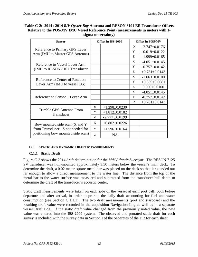
Data Acquisition and Processing Report Leidos Doc 15-TR-003
Project No. OPR-J312-KR-14 42 01/16/2015
Table C-2: 2014 / 2014 R/V Oyster Bay Antenna and RESON 8101 ER Transducer Offsets Relative to the POS/MV IMU Vessel Reference Point (measurements in meters with 1-
sigma uncertainty)
Sensor Offset in ISS-2000 Offset in POS/MV
Reference to Primary GPS Lever Arm (IMU to Master GPS Antenna)
X -2.7470.0176
Y -0.0190.0122
Z -1.9990.0165
Reference to Vessel Lever Arm (IMU to RESON 8101 Transducer
X -4.0510.0145
Y -0.7570.0142
Z +0.7810.0143
Reference to Center of Rotation Lever Arm (IMU to vessel CG)
X -1.6630.0100
Y +0.8390.0081
Z 0.0000.0100
Reference to Sensor 1 Lever Arm
X -4.0510.0145
Y -0.7570.0142
Z +0.7810.0143
Trimble GPS Antenna From Transducer
X +1.2980.0230
Y +1.8120.0182
Z -2.777 0.0199
Bow mounted side scan (X and Y from Transducer. Z not needed for positioning bow mounted side scan)
X +6.8020.0226
Y +1.5960.0164
Z NA
C.1 STATIC AND DYNAMIC DRAFT MEASUREMENTS
C.1.1 Static Draft
Figure C-3 shows the 2014 draft determination for the M/V Atlantic Surveyor. The RESON 7125 SV transducer was hull-mounted approximately 3.50 meters below the vessel’s main deck. To determine the draft, a 0.02 meter square metal bar was placed on the deck so that it extended out far enough to allow a direct measurement to the water line. The distance from the top of the metal bar to the water surface was measured and subtracted from the transducer hull depth to determine the draft of the transducer’s acoustic center. Static draft measurements were taken on each side of the vessel at each port call; both before departure and after arrival, in order to prorate the daily draft accounting for fuel and water consumption (see Section C.1.1.1). The two draft measurements (port and starboard) and the resulting draft value were recorded in the acquisition Navigation Log as well as in a separate vessel Draft Log. If the static draft value changed from the previously noted value, the new value was entered into the ISS-2000 system. The observed and prorated static draft for each survey is included with the survey data in Section I of the Separates of the DR for each sheet.

Data Acqu
Project No
Figure Ctransducedeterminapproximline. Thfrom the Static dradraft meaLog as wpreviouslstatic draDR for e
Fi
uisition and Pro
o. OPR-J312-K
Figure C
C-4 shows ther was pole-
ne the drafmately even he distance f
transducer d
aft measuremasurements well as in aly noted valaft for each ach sheet.
igure C-4: 2
ocessing Repor
KR-14
C-3: 2014 M
he 2014 draf-mounted apft, a referewith the po
from the refedepth to dete
ments were and each rea separate vlue, the newsurvey is in
2014 / 2014
rt
M/V Atlantic
ft determinatpproximatelyence point ort side deckference pointermine the dr
taken daily,sulting draft
vessel Draftw value wascluded with
R/V Oyster
43
Surveyor 71
tion for the y 1.31 meter
was establk, which allot to the watraft of the tr
, both beforft value weret Log. If ths entered int
the survey
Bay RESO
125 SV Draf
R/V Oyster rs below thelished on towed a direcer surface w
ransducer’s a
re departure e recorded ihe static drto the ISS-2data in Sect
N 8101 ER
L
ft Determin
Bay. The Re vessel’s pothe transduct measurem
was measureacoustic cent
and after arin the acquisraft value ch2000 systemtion I of the
Draft Deter
Leidos Doc 15
01/16
nation
RESON 810ort side deckucer pole-mment to the wed and subtrter.
rrival. The sition Navighanged from
m. The obsee Separates o
rmination
5-TR-003
6/2015
01 ER k. To
mount, water racted
daily gation m the erved of the

Data Acquisition and Processing Report Leidos Doc 15-TR-003
Project No. OPR-J312-KR-14 44 01/16/2015
C.1.1.1 Prorated Static Draft
An initial processing step of the Leidos data processing pipeline is to apply, if necessary, prorated static draft values to all bathymetric data. This was done to account for the change in the survey vessel draft during consecutive survey days, primarily due to fuel and water consumption. For these survey operations, Leidos only implemented the prorated static draft procedure for multibeam data collected by the M/V Atlantic Surveyor. As mentioned in Section C.1.1, the static draft was measured and recorded both prior to departure for the survey site, and immediately upon arrival to port after each survey leg. These two observed static draft measurements for each survey leg were then used to calculate the amount of change in the vessel static draft (in meters) observed over that survey leg. For a given period of survey, the change in vessel static draft divided by the number of consecutive days of survey resulted in the amount of change in vessel static draft per day. This daily change in the static draft was then subtracted from the observed static draft value at the beginning of that specific period of survey. This resulted in a unique prorated static draft value for each consecutive survey day that was then applied to the data for that day. When the JD rollover occurs in the middle of a survey line, the first file of the new day will be given the same prorated draft as the previous day. This procedure ensures that the static draft for every survey line is constant and does not cause a vertical jump in the survey depths. This method was only used when continuous survey operations were conducted between the static draft measurements observed immediately prior to departure and immediately upon arrival to port. It assumed a constant amount of fuel and onboard water was consumed per day of continuous survey operations, thereby providing the ability to calculate a constant rate of change in the survey vessel draft per day. The Apply Correctors Offsets tool within SABER was then used to apply the calculated prorated draft value for a given JD to all data within the multibeam GSF files of that specific JD. This process of applying a new prorated draft offset to the multibeam data was captured within the history record of each multibeam GSF file. Once prorated static draft had been applied to the multibeam data for a JD, the Apply Correctors Offsets tool within SABER was then used to report all the current offsets applied to the data within the multibeam GSF files of that JD. This was done to ensure the expected prorated static draft value was correctly applied to all multibeam data for that day. In addition, the history record of the multibeam GSF files was reviewed to ensure the process of applying prorated draft was captured and done correctly. The observed and prorated static draft for each survey is included with the survey data in Section I of the Separates of each sheet’s Descriptive Report. The static draft applied to each individual GSF file is reported in the Multibeam Processing Log for each sheet.

Data Acquisition and Processing Report Leidos Doc 15-TR-003
Project No. OPR-J312-KR-14 45 01/16/2015
C.1.2 Dynamic Draft
Dynamic draft values were confirmed during the sea acceptance tests (SAT) performed for each survey vessel (see Appendix I for details). For the M/V Atlantic Surveyor Table C-3 summarizes the shaft RPM, depth corrector, approximate speed, and the 2014 SAT multibeam files used to confirm the dynamic draft values (JD 175). The values determined from the analysis were entered into a look up table within the ISS-2000 system. A shaft RPM counter provided automatic input to the ISS-2000 system, which in conjunction with the look up table, applied a continuously updated dynamic settlement and squat value as data were collected.
Table C-3: 2014 M/V Atlantic Surveyor Settlement and Squat Confirmation
RPM FILENAME SQUAT
CORRECTOR USED
DELTA FROM DIFFERENCE
GRIDS 1-SIGMA
0 asmba14175.d37 0.00 NA NA
140 asmba14175.d03
0.00 -0.002 0.034509 asmba14175.d04
180 asmba14175.d05
0.02 -0.030 0.018750 asmba14175.d06
250 asmba14175.d07
0.03 +0.038 0.014506 asmba14175.d08
300 asmba14175.d09
0.06 -0.007 0.013403 asmba14175.d10
340 asmba14175.d11
0.09 +0.013 0.014511 asmba14175.d12
380 asmba14175.d13
0.11 +0.019 0.015689 asmba14175.d14
AVERAGE STANDARD DEVIATION 0.048880 For the R/V Oyster Bay Table C-4 and Table C-5 summarizes the engine RPM, depth corrector, approximate speed, and the 2014 SAT multibeam files used to determine dynamic draft values (JD 192, 193, and 199). Table C-6 summarizes the final correctors used for 2014. The values determined from the analysis were entered into a look up table within the ISS-2000 system. An engine RPM counter with digital display provided RPM values to the vessel captain and the hydrographer. The RPM value in use was then manually input into the ISS-2000 system, which in conjunction with the look up table, applied a continuously updated dynamic settlement and squat value as data were collected.
Table C-4: 2014 R/V Oyster Bay Settlement and Squat Determination on Julian Days 192 and 193
Engine RPM MB Files (JD192) Depth Corrector MB Files (JD193) Depth Corrector 0 obmba14192.d22 N/A obmba14193.d24 N/A
600 obmba14192.d23 obmba14192.d24
0.020 obmba14193.d25 obmba14193.d26
0.025
1600 obmba14192.d25 obmba14192.d26
-0.017 obmba14193.d99 obmba14193.d27
0.000
2000 obmba14192.d27 0.014 obmba14193.d28 -0.002

Data Acquisition and Processing Report Leidos Doc 15-TR-003
Project No. OPR-J312-KR-14 46 01/16/2015
Engine RPM MB Files (JD192) Depth Corrector MB Files (JD193) Depth Corrector obmba14192.d28 obmba14193.d29
2400 obmba14192.d29 obmba14192.d30
0.025 obmba14193.d30 obmba14193.d31
0.021
Table C-5: 2014 R/V Oyster Bay Settlement and Squat Determination on Julian Day 199
Engine RPM MB Files (JD199) Depth Corrector MB Files (JD199) Depth Corrector 0 obmba14199.D47 N/A obmba14199.D47 N/A
600 obmba14199.D48 obmba14199.D49
0.015 obmba14199.D56 obmba14199.D57
0.020
1600 obmba14199.D99 obmba14199.D98
0.001 obmba14199.D58 obmba14199.D59
0.002
2000 obmba14199.D50 obmba14199.D51
0.004 obmba14199.D60 obmba14199.D61
-0.012
2400 obmba14199.D53 obmba14199.D54
-0.024 obmba14199.D62 obmba14199.D63
-0.017
Table C-6: Final R/V Oyster Bay Settlement and Squat Correctors for.2014
Engine RPM New Jersey Alabama Final
Corrector JD 192 JD 193 JD 199 Run 1 JD 199 Run 2
0 N/A N/A N/A N/A N/A
600 0.020 0.025 0.015 0.020 0.02
1600 -0.017 0.000 0.001 0.002 0.00
2000 -0.014 0.012 0.004 -0.012 0.00
2400 -0.025 -0.021 -0.024 -0.017 -0.02
C.1.3 Speed of Sound
A Moving Vessel Profiler (MVP) manufactured by Brooke Ocean Technology Ltd., with an Applied Microsystems Ltd. Smart Sound Velocity and Pressure (SV&P) sensor, as well separate Seabird Electronics SBE-19 CTD sensors were used to determine sound speed profiles for corrections to multibeam sonar soundings. Confidence checks were obtained periodically (every 6-13 days) two consecutive casts taken with different SV&P sensors, with a SV&P sensor and a Seabird SBE-19 CTD, or between two different Seabird SBE-19 CTDs. After downloading the sound speed profile (SSP) comparison casts, graphs and tabulated lists were used to compare the two casts. During multibeam acquisition, SSP casts were uploaded to ISS-2000 immediately after they were taken. In ISS-2000, the profiles were reviewed for quality, edited as necessary, compared to the preceding casts, and then applied (loaded into the multibeam system for use). Once applied, the multibeam system used the profile data for depth calculation and ray tracing corrections to the multibeam data. If sounding depths exceeded the cast depth, the ISS-2000 used the deepest sound speed value of the profile to extend the profile to the maximum depth.

Data Acquisition and Processing Report Leidos Doc 15-TR-003
Project No. OPR-J312-KR-14 47 01/16/2015
Factors considered in determining how often a SSP cast was needed included shape and proximity of the coastline, sources and proximity of freshwater, seasonal changes, wind, sea state, water depth, observed changes from the previous profiles, and differences in the surface sound speed of the current profile compared to a separate surface sound speed sensor collocated with the multibeam sonar. At a minimum, for survey operations on the M/V Atlantic Surveyor SSP casts were taken at the beginning of each survey leg, at approximately two-hour intervals, and at the end of each survey leg. During daily survey operations for the R/V Oyster Bay, SSP casts were taken, at a minimum, before the start of bathymetric data acquisition, midway through the survey day, and at the end of bathymetric data collection for each survey day. Quality control tools in ISS-2000, including real-time displays of color-coded coverage and a multibeam swath waterfall display, were used to monitor how the sound speed affected the multibeam data. By using these techniques any severe effects due to sound speed profiling could be seen when viewing multibeam data in an along-track direction. Proper sound speed application and effects were also analyzed throughout the survey during post processing using the Leidos Analyze Crossings software and by PFM review of final uncertainties. A Sound Speed Profile Log including details of all SSP casts (such as date, location, application times, and maximum depth) is located in Separates II of the DR for each sheet. These Logs are separated by the purpose of the applied cast, categorizing each SSP file as “Used_for_Bathymetry” (applied to online bathymetry data), “Used_for_Closing” (a separate cast applied at the end of a survey leg immediately after online data collection needed for TPU calculations), “Used_for_Comparison”, and “Used_for_Lead_Line”. Additionally, there are sound speed profile files (.svp) in a separate folder on the delivery drive; “HXXXXX/Data/Processed/SVP/CARIS_SSP”. These files contain concatenated SSP data that has been formatted for use in CARIS. The CARIS SSP files are designated based on the type of sensor and the purpose of the cast and their filenames match the tabs within the sound speed profile log.
C.2 MULTIBEAM CALIBRATIONS
A Sea Acceptance Test (SAT) was conducted independently for each survey vessel and sonar installation, prior to the start of each vessel’s data acquisition on this project. The SAT for the M/V Atlantic Surveyor integrated with the RESON 7125 SV multibeam system was conducted from 19 June 2014 (JD 169) to 25 June 2014 (JD 176) in New Jersey and the results verified in Alabama on 09 July 2014 (JD 190). The SAT for the R/V Oyster Bay was conducted from 10 July 2014 (JD 191) to 13 July 2014 (JD 194) in New Jersey and the results verified in Alabama on 18 July 2014 (JD 199). Navigation positioning, heading, heave, roll, and pitch were provided by the Applanix POS/MV 320 Inertial Navigation System. Resolution and accuracy of this system are:
Heave Resolution 1 cm, Accuracy greater of 5 cm or 5% of heave amplitude Roll Resolution 0.01º, Accuracy 0.02º Pitch Resolution 0.01º, Accuracy 0.02º

Data Acqu
Project No
The Appprocessin
C.2.1
A ping tithat no tiwas the characterline of thtrigger odemonstr1.5 millis
Figure
A ping tion 02 JuAppendixBC635PC(TTL) pupulses offrom the correspon
uisition and Pro
o. OPR-J312-K
planix TrueHng (see Secti
1 Timing T
iming test foiming errorsevent markirized by a phe IRIG-B cof the RESOrated that alseconds (Fig
C-5: 21 Ju
iming test fouly 2014 (JDx II). The CI IRIG-B culse occurrinf interest wePOS/MV. Tnding IRIG-
ocessing Repor
KR-14
Heave™ option C.3 for d
Test
or the RESOs existed witing capabilitositive-goinonnector onON 7-P anl GSF ping
gure C-5).
ne 2014 REtrigge
or the RESOND 183) to ver
fundamentacard. An eveng on the evere the transmThese tests d-B event time
rt
tion was usdetails of del
ON 7125 SVthin the survty of the Sy
ng transistor-n the back ofnd the 1PPS
times match
ESON 7125 Ser event vs. p
N 8101 ER rify that no
al tool was ent is charac
vent line of tmit trigger odemonstratedes to within
48
ed to recordlayed heave
V was complvey system (ymmetricom-transistor lof the ISSC. S timing puhed the corre
SV Timing ping time ta
installed onbtiming errorthe event m
cterized by athe IRIG-B cof the RESOd that the av1.5 millisec
d delayed hand the appl
leted on 21 see Append
m BC635PCIogic (TTL) pThe pulses
ulses from esponding IR
Test Resultag from GS
board the R/rs existed w
marking capa positive-goconnector on
ON 8101 ERverage of all onds (Figure
L
heave for aplication proc
June 2014 (dix II). The I IRIG-B capulse occurrof interest wthe POS/MRIG-B even
ts (time diffF)
/V Oyster Bawithin the supability of thoing transiston the back o
R and the 1PGSF ping ti
e C-6).
Leidos Doc 15
01/16
pplication incess).
(JD172) to vfundamenta
ard. An evering on the were the tran
MV. These nt times to w
ferences of p
ay was compurvey systemhe Symmetror-transistor of the ISSC. PPS timing pimes matche
5-TR-003
6/2015
n post
verify al tool ent is event nsmit tests
within
ping
pleted m (see ricom logic The
pulses ed the

Data Acqu
Project No
Figure
C.2.2
Roll, pitcJune 201Appendixupon arrTable C-
TabAlign
uisition and Pro
o. OPR-J312-K
C-6: 02 Ju
2 Multibea
ch, and head14 (JD175) x II for detaival in Alab8.
ble C-7: Munment Tool
Componen
Pitch
Roll
Gyro
ocessing Repor
KR-14
uly 2014 REtrigge
am Bias Cal
ding biases wfor the RE
ails). The rebama on 09
ultibeam Fil(SAT) – 23
nt
asm
asm
asm
rt
SON 8101 Eer event vs. p
ibration (Al
were determiESON 7125esults are pre
July 2014 (
les VerifyinJune 2014
Mult
mba14175.d18
mba14175.d18
mba14175.d20
49
ER Timing ping time ta
lignment)
ined on 23 J SV installesented in T(JD 190). T
g AlignmenRESON 712
tibeam files
asmba
asmba
asmba
Test Resultag from GS
June 2014 (Jled on the
Table C-7. TThe verifica
nt Bias Calc25 SV on th
a14175.d19
a14175.d19
a14175.d21
L
ts (time diffeF)
JD 174) and M/V Atlanti
The bias resuation results
culated usinghe M/V Atlan
Resu
+1.0
+0.32
+0.
Leidos Doc 15
01/16
ferences of p
confirmed oic Surveyorults were verare present
g the Swathntic Surveyo
ult
00°
29°
8°
5-TR-003
6/2015
ping
on 24 r (see rified ted in
h or

Data Acquisition and Processing Report Leidos Doc 15-TR-003
Project No. OPR-J312-KR-14 50 01/16/2015
Table C-8: Multibeam Files Verifying Alignment Bias Calculated using the Swath Alignment Tool (SAT) – 09 July 2014 RESON 7125 SV on the M/V Atlantic Surveyor
Component Multibeam files Result
Pitch asmba14190.d20 asmba14190.d21 +1.00°
Roll asmba14190.d20 asmba14190.d21 +0.329°
Gyro asmba14190.d23 asmba14190.d25 +0.8°
Roll, pitch, and heading biases were determined on 12 July 2014 (JD 193) for the RESON 8101 ER installed on the R/V Oyster Bay (see Appendix II for details). The results are presented in Table C-9. Offsets determined on JD 193 were verified on 18 July 2014 (JD 199) upon arrival in Alabama. The verification results are presented in Table C-10.
Table C-9 Multibeam Files Verifying Alignment Bias Calculated using the Swath Alignment Tool (SAT) – 12 July 2014 RESON 8101 ER on the R/V Oyster Bay
Component Multibeam Files Bias
Pitch OBMBA14193.d04 OBMBA14193.d05 +0.07°
Roll OBMBA14193.d33 OBMBA14193.d34 -1.30°
Heading OBMBA14193.d37 OBMBA14193.d38 -0.20°
Table C-10: Multibeam Files Verifying Alignment Bias Calculated using the Swath Alignment Tool (SAT) – 18 July 2014 RESON 8101 ER on the R/V Oyster Bay
Component Multibeam Files Bias
Pitch OBMBA14199.d12 OBMBA14199.d13 +0.07°
Roll OBMBA14199.d12 OBMBA14199.d13 -1.30°
Heading OBMBA14199.d19 OBMBA14199.d20 -0.20°
C.2.3 Multibeam Accuracy
During the June 2014 SAT of the M/V Atlantic Surveyor, a survey was run to analyze multibeam accuracies with the RESON 7125 SV (see Appendix II for details). The survey was run in the vicinity of a 47 foot wreck in the fish haven approximately 6 kilometers southeast of Manasquan Inlet. The wreck is located in 40° 03.3925’N 073° 59.5541’W. All depths were corrected for predicted tides and zoning using the Atlantic City tide gage, 8534720. The class 1 cutoff angle was set to 5° and the class 2 cutoff angle was set to 60°. The multibeam was configured for 256 Equi-Angular beams. Standard multibeam data processing procedures were followed to clean the data, apply delayed heave, and calculate errors. One-meter minimum grids of main scheme lines, class 1 crosslines, and all lines were created and analyzed. A two-meter PFM of all the data was also generated and the Gapchecker and Check Uncertainty routines were run on the PFM CUBE depth layer. Multibeam features, side scan contacts, and selected soundings in feet were generated.

Data Acquisition and Processing Report Leidos Doc 15-TR-003
Project No. OPR-J312-KR-14 51 01/16/2015
During the June 2014 SAT of the R/V Oyster Bay, a survey was run to analyze multibeam accuracies with the RESON 8101 (see Appendix II for details). The survey was run in the vicinity of a 47 foot wreck in the fish haven approximately 6 kilometers southeast of Manasquan Inlet. The wreck is located in 40° 03.3925’N 073° 59.5541’W. All depths were corrected for predicted tides and zoning using the Atlantic City tide gage, 8534720. The class 1 cutoff angle was set to 5° and the class 2 cutoff angle was set to 60°. Standard multibeam data processing procedures were followed to clean the data, apply delayed heave, and calculate errors. One-meter minimum grids of main scheme lines, class 1 crosslines, and all lines were created and analyzed. Additionally common data from both systems were compared and analyzed against each other. The results showed that both systems met the uncertainty standards stated in Section 5.1.3 of the HSSD. On 06 August 2014 (JD218), during survey operations, a confidence check of the multibeam systems was made by comparing the depth data collected over a common survey line which was run simultaneously by the R/V Oyster Bay and the M/V Atlantic Surveyor. For this multibeam comparison both vessels met, took and applied individual SSP casts, and then proceeded to acquire data over a common survey line, one vessel immediately following the other to reduce any tidal or environmental differences. The data acquired over this common survey line were fully processed following standard bathymetric data processing procedures to clean the data, apply delayed heave, apply pro-rated draft, apply verified tide correctors, and calculate errors. Separate two-meter PFM grids of the data from each were generated. Difference grids were generated between the individual PFM CUBE Depth layers and SABER Frequency Distribution tool was used to analyze the difference layer. The results from the differences between the M/V Atlantic Surveyor and the R/V Oyster Bay showed that 97.37% of the soundings compared to within 0.10 meters as shown in Table C-11. Depth differences were also symmetrically centered on zero as shown in Figure C-7. All results showed that the systems met the accuracy and uncertainty standards stated in Section 5.1.3 of the HSSD.

D
P
T
Data Acquisition an
Project No. OPR-J
Table C-11: Fr
Depth Difference(meters)
0.0-0.1 >0.1-0.2 >0.2-0.3 >0.3-0.4
>0.4-0.435
Total
Figure C-7: F
nd Processing Rep
J312-KR-14
requency Distr
e Bins Cumulat
Percen
36291 97.37 958 99.94 20 100.000 100.00
5 1 100.00
37270 100.00
Frequency Dist
port
ribution of Dep
Gri
tive nt
Percentile Po
B
100.00 12.63 9
0 0.06 0 0.00 0 0.00
0 0.00 1
tribution Grap
pth Differences
id: asmba14218_d24_2
ositive Bins
Positive Cumulative
Percent
5163 40.68 916 43.14 20 43.20 0 43.20 0 43.20
6099 43.20
ph of Depth DiffCo
52
between the MLine
2m_pfm_obmba14218
Positive Percentile
NegativBins
43.20 206572.51 420.05 0 0.00 0 0.00 1
0.00 20700
fferences betweommon Line
M/V Atlantic Sur
8_d03_2m_pfm.dif
ve Negative
Cumulative Percent
NP
7 55.43 55.54 55.54 55.54 55.54
0 55.54
een the M/V Atl
rveyor and the
Negative Percentile
Zero Bins
55.54 471 0.12 0.00 0.00 0.00
0.00 471
lantic Surveyor
Leidos Doc 1
R/V Oyster Bay
Zero Cumulative
Percent
ZeroPercen
1.26 0.00
1.26 0.00
and the R/V Oy
5-TR-003
01/16/2015
y Common
o ntile
0
0
Oyster Bay

Data Acquisition and Processing Report Leidos Doc 15-TR-003
Project No. OPR-J312-KR-14 53 01/16/2015
C.3 DELAYED HEAVE
As discussed in Section B.2, Leidos and SABER use the terminology delayed heave to describe Applanix TrueHeave™ data collected from the Applanix POS/MV. At the start of all survey operations, the Applanix POS/MV was configured to log TrueHeave™ data. The delayed heave files (.thv) were recorded using ISS-2000 and archived to the NAS or external hard drive in the same manner as GSF files. The delayed heave data were calculated by the Applanix POS/MV based on an algorithm which used a range of temporally bounding Applanix POS/MV real-time heave data to produce a more accurate value of heave. When the resulting delayed heave values were applied to the multibeam data they reduced heave artifacts present from variables such as sea state and survey vessel maneuvering, which are commonly observed in multibeam data with only real-time heave applied. When delayed heave corrections were applied to the bathymetric data, each depth value was fully recalculated in SABER. This was possible because the raw beam angle and travel time values were recorded in the GSF file. The raw beam angle and travel time values were used along with the vessel attitude (including heave) and re-ray traced. As delayed heave was applied, a history record was written to each GSF file, and the ping flag of each modified ping was updated. After the application of delayed heave was complete, all bathymetric data were reviewed to verify that the delayed heave values were applied using the SABER command line program check_heave. This program read through the ping flags of each GSF record to check the application of delayed heave. When the check_heave program found instances where delayed heave was not applied, it output report files which included the GSF filename, as well as the time range for the gap in delayed heave application. The data from the check_heave reports was then used to further investigate all instances of gaps in delayed heave application. Leidos strived to have delayed heave applied to all soundings of multibeam data, however there were times when this was not possible. Real-time heave was used in place of delayed heave in all instances where there were gaps in the application of delayed heave. All gaps in delayed heave application were fully investigated and the data reviewed to verify that the real-time heave values were appropriate to the surrounding available delayed heave values. Any instances where the absence of delayed heave adversely affected the data will be discussed in the DR for the respective sheet.
C.4 TIDES AND WATER LEVELS
NOAA tide stations 8741533 Pascagoula, MS and 8735180 Dauphin Island, AL were specified in the OPR-J312-KR-14 Project Instructions to be used as the sources for water level correctors for these surveys. Included with the Project Instructions was a Statement of Work for the Tides and Water Levels (11/25/2013 HY). Leidos received the zoning information in a CARIS Zone Definition File format (.zdf) and MapInfo data files. Leidos used SABER Survey Planning to create tide zone files (.zne) based on the positional data provided from the *.zdf files, for use within ISS-2000 and SABER.

Data Acquisition and Processing Report Leidos Doc 15-TR-003
Project No. OPR-J312-KR-14 54 01/16/2015
All tide data for the project were downloaded, as text files (.txt), from the NOAA Center for Operational Oceanographic Products and Services (CO-OPS) Tides & Currents website. Predicted tide levels were used for real-time data acquisition and observed verified tides were later downloaded for the computation of the final water level correctors. All 6-minute water level data were in meters and annotated with the Coordinated Universal Time (UTC). The SABER Create Water Level Files tool was used to generate the final water level files for each tide zone. This tool generates a Tide Zone Parameters (.tzp) file and water level files. The Tide Zone Parameter file contains time offset and range ratio information for each of the tide zones within the survey area. These values were obtained from NOAA and are listed in Table C-12. Leidos did not modify any of these parameters. Once the *.tzp file is generated it is used to create water level files. These files were created based on the data input from the downloaded predicted or verified tide data that was saved as a text file. SABER outputs the water level files by zone with a file extension corresponding to the type of data (predicted or verified) were within the input text file. For example, CGM29.ov is a water level file for Zone CGM29 that includes verified water level data. These water level files were applied to the multibeam data using the SABER Apply Tides program. This program took the water level heights contained within the water level files and algebraically subtracted them from surveyed depths to correct each sounding for tides. When updated water level correctors (such as verified tides) were applied to the GSF files, the program removed the previous water level corrector and applied the new corrector. Each time the program was run on the GSF files, a history record was appended to the end of the GSF file documenting the date and water level files applied. For quality assurance, the SABER Check Tide Corrections in GSF program was run on all GSF files to confirm that the appropriate water level corrector had been applied to the final GSF files. The primary means for analyzing the adequacy of the correctors was observing zone boundary crossings in SABER’s MultiView Editor. After confirmation that verified water levels were applied to all bathymetric data, grids were created and analyzed using various color change intervals and shaded relief. The color intervals and shaded relief provided a means to check for significant, unnatural changes in depth across zone boundaries due to water level correction errors, unusual currents, storm surges, etc. In addition, crossline analysis using the SABER Junction Analysis routine was run and the results of the SABER Frequency Distribution tool were analyzed and used to identify possible depth discrepancies resulting from the applied water level correctors. Discrepancies were further analyzed to determine if they were the result of incorrect zoning parameters or weather (wind) conditions between the tide station and the survey area. No final tide note was provided by the NOAA Center for Operational Oceanographic Products and Services (CO-OPS). Leidos is not required to have a final tide note from CO-OPS for OPR-J312-KR-14. Additionally, in a separate folder on the delivery drive for each sheet, in the “HXXXXX/Data/Processed/Tide/CARIS_Tide_Files” folder, are support files for use in CARIS. Leidos created each CARIS Tide File (*.tid) using the same observed verified water level data

Data Acqu
Project No
downloadobservedreformattDefinitioWork (11
C.4.1
All surveCGM38,CGM44,(Figure CDauphin
Figure C
uisition and Pro
o. OPR-J312-K
ded from thd verified wted to meet t
on File (J311/25/2013 H
1 Final Tid
eys were conCGM38A,
CGM44A, C-8) which aIsland, AL.
C-8: Tide Z
ocessing Repor
KR-14
he NOAA Cwater level the file struc2KR2014CO
HY).
de Note
ntained with, CGM39, CGM45, C
are reference The NOAA
ones for Sta
rt
CO-OPS Tiddata files (
cture used inORP.zdf), w
hin preliminCGM40, CGM46, CGM
ed to NOAAA provided z
ations 87415H12655, H1
55
es & Curren*.ov) used
n CARIS. Awhich Leido
nary water leCGM40A, CM46A, CGM
A tide stationzoning param
533 and 87312656, and H
nts websitein SABER
Also includedos received
evel zones CCGM41, CGM47, CGM4ns 8741533 Pmeters are pr
35180 CoverH12657
L
that is usedR. Then thd in this direwith the tid
CGM29, CGGM42, CGM48, CGM122Pascagoula, resented in T
ring Survey
Leidos Doc 15
01/16
d for creatinhe *.tid fileectory is the des Stateme
GM37, CGMM42A, CG2, GB2 and MS and 873
Table C-12.
y Areas H12
5-TR-003
6/2015
ng the e was Zone
ent of
M37A, M43, GB3
35180
2654,

Data Acquisition and Processing Report Leidos Doc 15-TR-003
Project No. OPR-J312-KR-14 56 01/16/2015
Table C-12: Preliminary Tide Zone Parameters
Zone Time Corrector (minutes)
Range Ratio Reference Station
CGM29 -78 x0.88 8741533
CGM37 -66 x0.88 8741533
CGM37A -54 x0.88 8741533
CGM38 -48 x0.88 8741533
CGM38A -42 x0.88 8741533
CGM39 -36 x0.88 8741533
CGM40 -24 x0.88 8741533
CGM40A -30 x0.88 8741533
CGM41 -54 x1.08 8735180
CGM42 -42 x1.08 8735180
CGM42A -36 1.04 8735180
CGM43 -24 1.04 8735180
CGM 44 -18 1.04 8735180
CGM44A -12 x1.00 8735180
CGM45 0 x1.00 8735180
CGM46 +6 x1.04 8735180
CGM46A +12 x1.13 8735180
CGM47 +18 x1.17 8735180
CGM48 +24 x1.17 8735180 CGM122 -30 x0.94 8741533
GB2 -18 x1.01 8741533 GB3 -24 x1.01 8741533
The verified water level correctors were computed at six minute intervals for each zone and referenced to the Mean Lower-Low Water (MLLW) vertical datum. Analysis of the bathymetric data in MVE and in depth grids revealed minimal depth changes across the junction of the zones. A spreadsheet analysis of the water level correctors for each zone and the differences observed at the boundaries of adjacent zones also confirmed the adequacy of zoning correctors based on 8741533 Pascagoula, MS and 8735180 Dauphin Island, AL. For the zone junction analysis, observed verified water levels from 01 July 2014 (JD213) through 12 October 2014 (JD026) were entered into a spreadsheet and the differences between adjacent zones are summarized in Table C-13.

Data Acquisition and Processing Report Leidos Doc 15-TR-003
Project No. OPR-J312-KR-14 57 01/16/2015
Table C-13: 2014 Differences in Water Level Correctors between Adjacent Zones Using Zoning Parameters for Stations 8741533 and 8735180
Zone Boundary Minimum Difference
Maximum Difference
Average Difference
Standard Deviation
CGM29 – CGM37 -0.088 0.074 0.000 0.009
CGM37 – CGM37A -0.088 0.074 0.000 0.009
CGM37A – CGM38 -0.057 0.057 0.000 0.005
CGM38 – CGM38A -0.057 0.057 0.000 0.005
CGM38A – CGM39 -0.057 0.057 0.000 0.005
CGM 38A – CGM122 -0.099 0.065 -0.021 0.014
CGM39 – CGM40 -0.088 0.074 0.000 0.009
CGM39 – CGM122 -0.08. 0.035 -0.021 0.012
CGM40 – CGM40A -0.057 0.057 0.000 0.005
CGM40A – CGM41 -0.198 0.230 -0.010 0.039
CGM41 – CGM42 -0.131 0.120 0.000 0.014
CGM41 – GB3 -0.252 0.289 -0.036 0.040
CGM42 – CGM42A -0.152 0.123 0.012 0.013
CGM42 – GM3 -0.260 0.201 -0.036 0.040
CGM42A – CGM43 -0.126 0.115 0.000 0.013
CGM42A – CGM45 -0.151 0.135 0.012 0.025
CGM42A – GB3 -0.256 0.197 -0.048 0.042
CGM43 – CGM44 -0.158 0.112 0.000 0.011
CGM43 – CGM45 -0.139 0.133 0.012 0.019
CGM43 – GB3 -0.285 0.213 -0.048 0.043
CGM44 – CGM44A -0.145 0.119 0.012 0.012
CGM44 – CGM45 -0.147 0.142 0.012 0.016
CGM44 – GB3 -0.282 0.218 -0.048 0.044
CGM44A – CGM45 -0.121 0.111 0.000 0.013
CGM44A – GB2 -0.291 0.229 -0.059 0.049
CGM45 – CGM46 -0.165 0.101 -0.012 0.012
CGM45 – GB2 -0.291 0.229 -0.059 0.049
CGM46 – CGM46A -0.187 0.097 -0.027 0.018
CGM46 – CGM47 -0.166 0.093 -0.038 0.024
CGM46 – GB2 -0.272 0.229 -0.048 0.049
CGM46A – CGM47 -0.184 0.155 -0.012 0.013
CGM47 – CGM48 -0.177 0.126 0.000 0.012
CGM47 – GB2 -0.234 0.240 -0.009 0.054
As a result, the NOAA preliminary zone boundaries and zoning parameters for 8741533 Pascagoula, MS and 8735180 Dauphin Island, AL were accepted as final and applied to all multibeam data.

Data Acquisition and Processing Report Leidos Doc 15-TR-003
Project No. OPR-J312-KR-14 01/16/2015
D. APPROVAL SHEET
16 January 2015 LETTER OF APPROVAL REGISTRY NUMBER: H12654, H12655, H12656 and H12657 Field operations and data processing contributing to the accomplishment of these surveys, H12654, H12655, H12656 and H12657, were conducted under my supervision and that of the other Leidos lead hydrographers with frequent personal checks of progress and adequacy. This report and accompanying deliverable data items have been closely reviewed and are considered complete and adequate as per the Statement of Work. This report and the accompanying digital data for project OPR-J312-KR-14, Approaches to Mobile Bay, are respectfully submitted. All records are forwarded for final review and processing. The survey data meets or exceeds requirements as set forth in the NOS Hydrographic Specifications Deliverables Manual. These data are adequate to supersede charted data in their common areas. Reports concurrently submitted to NOAA for this project include:
Report Submission Date H12654 Descriptive Report 16 January 2015
Gary R. Davis Chief Hydrographer
Leidos 16 January 2015