1

Dash for Cash: Month-End Liquidity Needs and the Predictability of Stock Returns 25 July 2015

Erkko Etula Kalle Rinne Goldman, Sachs & Co. University of Luxembourg Matti Suominen Lauri Vaittinen Aalto University School of Business Mandatum Life Abstract. We present broad-based evidence that the monthly cash needs of institutions induce systematic patterns in global stock returns. First, we document strong reversals in stock index returns around the last monthly trading day that guarantees cash settlement before month end. Second, we present direct evidence that links these reversals to institutional trading activity and funding conditions. Third, we find that the reversals are stronger for larger and more liquid stocks, and those more commonly held by mutual funds, a popular implementation vehicle among institutions. Finally, we show that mutual funds’ sensitivity to month-end reversals predicts their performance. Keywords: asset pricing, limits of arbitrage, mutual funds, short-term reversals, turn of the month effect JEL classification: G10, G12, G13

The views expressed in this paper are those of the authors and do not reflect the positions of Goldman, Sachs & Co or Mandatum Life.

We thank Huaizhi Chen, Thierry Foucault, Matti Keloharju, Dong Lou, Rajnish Mehra, Christopher Parsons, Joshua Pollet, Ioanid Rosu, Timo Somervuo, Hongjun Yan and seminar participants at Aalto University, HEC (Paris), the Luxembourg School of Finance, Mannheim University, the 8th Paul Woolley Centre Conference, and McGill University. Contact information. Erkko Etula: Goldman, Sachs & Co., 200 West Street, New York, NY 10282, Email: erkko.etula@gs.com, Tel: +1-617-319-7229; Kalle Rinne: Luxembourg School of Finance / University of Luxembourg, 4 Rue Albert Borschette, L-1246 Luxembourg, Luxembourg, E-mail: kalle.rinne@uni.lu, Tel: +352-46-66445274; Matti Suominen: Aalto University School of Business, P.O. Box 21210, FI-00076 Aalto, Finland, E-mail: matti.suominen@aalto.fi, Tel: +358-50-5245678, Fax: +358-9-43138678; Lauri Vaittinen: Mandatum Life, Bulevardi 56, 00120 Helsinki, Finland, Tel: +358 10 553 3336, Fax: +358 10 553 3275, E-mail: lauri.vaittinen@mandatumlife.fi. We are grateful to Joona Karlsson, Antti Lehtinen, Mikael Paaso, and Mounir Shal for excellent research assistance.

2

1. Introduction It is surprising how little attention academic literature has devoted to understanding equity market

returns around the turn of the month, despite the observations of Lakonishok and Smidt (1988) and

McConnell and Xu (2008), among others, that historically most of the returns have accrued during a

four-day period, from the last trading day to the third trading day of the month. Even less attention

has been paid to the fact that in more recent samples market returns are also abnormally high on the

last three trading days before the turn of the month. In fact, combining the two observations, we find

that since July 1926, one could have held the US value-weighted stock index (CRSP) for only seven

days a month and pocketed the entire market excess return with nearly fifty percent lower volatility

compared to a buy and hold strategy. The negative excess returns outside the seven day turn of the

month period are driven by dismal stock returns during the five trading days immediately before the

high turn of the month return period (see Figure 1).1 2

[INSERT FIGURE 1 HERE]

Following Ogden (1990), we argue that the origin of the turn of the month return patterns lies in the

monthly economic payment cycle – the fact that a disproportionate share of monthly payments in the

US economy, for instance those by pension funds (pensions), corporate treasuries (dividends), and

mutual funds (distributions), take place precisely at the turn of the month, as we document below.

Given this payment cycle, every month potentially billions of dollars invested in financial markets,

including the stock market, get first liquidated some time prior to the month end, then distributed as

cash payments to pensioners and investors at the month end, and finally partially re-invested in the

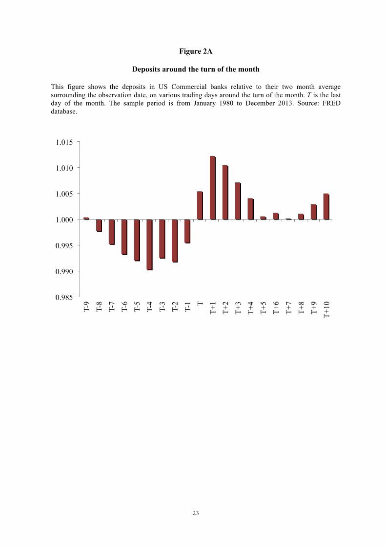
market by the recipients. Indeed, Figure 2A shows how deposits in US commercial banks rise visibly

on the last day of the month and decline rapidly after the first day of the month. The monthly

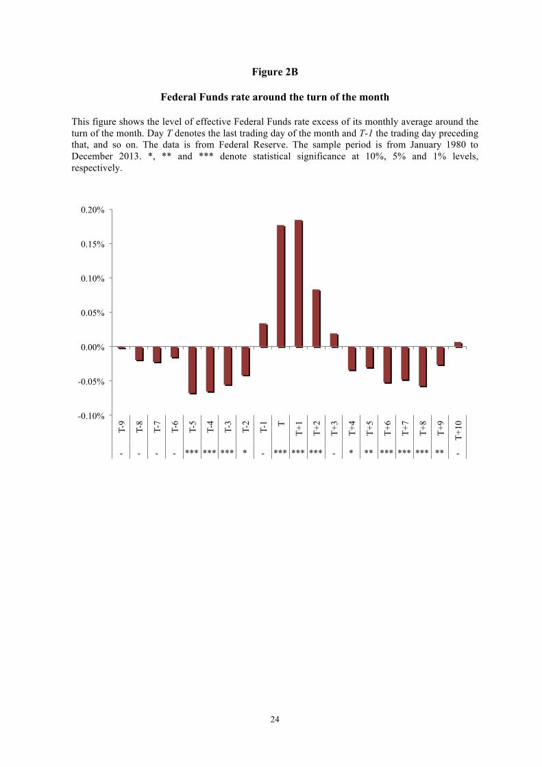
payment cycle, and the accompanying scarcity of cash at the month end, is also reflected in Figures

2B and 2C, which show sharp increases in the Fed Funds rate and the Libor rate on the last day of

the month.

[INSERT FIGURES 2A-C HERE]

Consistent with the payment cycle, we uncover strong return reversals in the aggregate stock market

around key dates near the turn of the month. In addition, we present empirical evidence that links

stocks’ turn of the month return patterns crisply to institutional investors’ buy-sell ratios, mutual

                                                                                                               1 We will henceforth refer to “trading days” simply as “days.” 2 McConnell and Xu (2008) and Cadsby and Ratner (1992) show that the turn of the month returns are high in most developed markets. Dzhabarov and Ziemba (2010) show that also US equity index futures exhibit a similar turn of the month effect.  

3

fund holdings, stock-level liquidity and volatility, and to capital market funding conditions. Time-

varying betas of mutual funds and hedge funds provide additional supporting evidence. Taken

together, our results suggest a coherent heuristic framework that ties the turn of the month return

patterns to the institutional payment cycle coupled with market-wide limits of arbitrage.

Our first observation is that, due to the 3-day settlement period in the US equity market (this

settlement period has also been the most common internationally), investors’ turn of the month

liquidity related selling of stocks must take place at least three days prior to the month end. Let us

label this critical day T-3, where T denotes the last day of the month. Under perfectly efficient

markets, market makers and speculators would ensure that prices are not affected by this type of

liquidity related sell orders, which do not reflect any investment views. However, in the absence of

sufficient speculative capital (see e.g. Grossman and Miller 1988; Gromb and Vayanos, 2002;

Brunnermeier and Pedersen, 2009), it is likely that market prices prior to T-3 get temporarily

depressed due to the selling pressure, and that it takes some time for the prices to revert back to their

fundamental values. This is the main hypothesis of our paper. As Ogden (1990) argues, in the

beginning of the month there should in turn be positive price pressure in the stock market as the

recipients of the month end cash payments invest new money into the stock market. Our second

hypothesis is therefore that the beginning of the month buying pressure temporarily elevates stock

prices above fundamentals, and that there is return reversal after the buying pressure subsides.3

Surprisingly, we find that many of the turn of the month return patterns that we document have

become more pronounced over time, and the strength of these phenomena seems to be related to the

proportion of institutional investors in the market. One potential explanation for this is that the

payments of institutions are particularly sharply clustered at the month end, as we document below.

A complementary explanation is related to intra-month variation in institutional risk appetite;

namely, that institutional investors avoid risk taking near the month end, for which we also find

some support in the data. Taken together, it is possible that the increased role of institutions has not

only led to additional selling pressure prior to T-3 (by the institutions with month end liquidity

needs), but also to a decreased willingness among market participants to accommodate selling

pressure near the month end. 4

Our empirical evidence on turn of the month return patterns and the role of institutions in the genesis

of these patterns can be divided into four main categories:

                                                                                                               3 Table 1 documents the dates when the 3-day settlement convention was adopted in different countries. In the US, the settlement period was shortened from 5 to 3 days in June 1995. See e.g. Thomas Murray Ltd. 2014 report “CMI In Focus: Equities Settlement Cycles.” 4 Window dressing ahead of reporting dates is a leading explanation for month-end risk reduction by mutual funds (e.g. Lakonishok, Shleifer, Thaler and Vishny, 1991).  

4

1. Evidence from market returns. Studying aggregate market prices alone, we find

significant predictability in stock market returns around the third business day before the

month end. The average market returns on the five business days preceding T-3 are negative,

in contrast to the subsequent three business days’ returns, which are highly positive. One of

our main findings is to show that lower than average market returns before T-3 tend to be

followed by higher than average subsequent returns, thus providing evidence of market

return reversals around T-3. Our evidence on return reversals around T-3 is not limited to the

US: In all 25 markets that we survey, there is evidence of return reversals around T-3, and in

22 of the 25 markets the return reversals are statistically significant. This evidence on return

reversals is consistent with the month-end payment cycle and limits of arbitrage, as

discussed earlier.5

2. Evidence from institutional investor trading data. To investigate the hypothesis that turn

of the month return patterns are in part driven by institutional investors’ liquidity-related

trading, we study a data set that contains trade-level observations for hundreds of different

institutional investors (mutual funds, hedge funds, pension funds, and other asset managers).

This ANcerno dataset (obtained from Abel Noser Solutions) is considered to be a highly

representative sample of institutional investors’ trading in the US stock market (e.g. Puckett

and Yan, 2011).

Our analysis reveals that there are indeed significant seasonalities in the relative tendency of

institutions to submit buy and sell orders. Consistent with our hypothesis, it appears that

institutions are net sellers in the market up to the morning of T-3 and net buyers on the last

day of the month and the first few days of the month. Moreover, we document using

regression analysis that greater aggregate institutional selling pressure on days T-8 to T-4

(normalized by the stock market capitalization) is associated with higher subsequent stock

market returns on days T-3 to T-1. These findings lend direct support to our hypothesis that

institutional trading affects stock returns around the turn of the month.

Combining the evidence on market returns and institutional investors’ trading patterns leads

us to conclude that institutions may incur significant costs from their liquidity-driven trading

                                                                                                               5 As a robustness check, to further test the idea that the payment cycle contributes to turn of the month patterns, we show in Table A1 in the Appendix that similar but less pronounced patterns in market returns in the US and elsewhere are observed around another common payment date, the 15th of each month. In addition, we find that in the US, the abnormally negative returns prior to the turn of the month have moved closer to the turn of the month since the shortening of the settlement period from four to three days in June 1995. Finally, the part of the seven-day turn of the month returns that accrue during the days T-3 to T-1 has significantly increased since the shortening of the settlement period (being on average 47% after June 1995 vs. 30% in the sample from January 1980 to May 1995).

5

at the month end. We estimate that the average costs associated with such trades may have

been over 0.4 billion US dollars per year from 1999 to 2010. These costs are eventually

borne by the pensioners and other investors that invest through these institutions.

3. Evidence related to mutual funds and the cross section of stocks. We further study the

link between institutional investors and turn of the month return patterns by using data on

mutual fund holdings and the cross-section of stock returns. We begin by linking month-end

return reversals at the stock level to mutual fund holdings. Our findings indicate that stocks

held in greater proportions by mutual funds exhibit more pronounced turn of the month

patterns: more negative returns between T-8 to T-4 and more positive returns from T-3 to T-

1. In addition, those stocks exhibit greater return reversals around T-3. Furthermore, in an

international sample, we find that the market-wide return reversals around T-3 are stronger

in countries with larger mutual fund sectors. Finally, we show that the strength of the return

reversal around T-3 in the US stock market has varied over time with the proportion of the

market held by the mutual fund industry.

Other pieces of evidence lend further support to the link between turn of the month return

patterns and mutual funds. For example, consistent with the idea that there are cash transfers

in and out of the mutual fund sector around the turn of the month, we find that the average

market beta of the mutual fund industry varies near the month end and is significantly lower

than average at time T-3. Furthermore, consistent with the idea that mutual funds reduce risk

toward the end of the month (either to increase their cash holdings for month-end payments

or for agency reasons), we find that mutual funds’ average return volatility declines toward

the month end although there is no observable coincident decline in market volatility.

We also find evidence that the turn of the month returns and return reversals vary as a

function of stock-level liquidity. In particular, we find that month-end reversals are more

significant for larger and more liquid stocks, which is consistent with the idea that turn of the

month patterns are tied to investors liquidity needs, and that investors respond to month-end

outflows and cash needs conscious of transaction costs.

Finally, we present evidence that mutual funds’ turn of the month trading patterns predict

their alpha. For instance, we find that the Carhart (1997) four-factor alpha is significantly

positive for the funds that exhibit the highest historical correlations in their T-8 to T-4 and T-

3 to T-1 returns, and negative for all other funds. We interpret this as complementary

evidence (to that obtained from ANcerno’s institutional trading data) that most institutions

suffer significantly from their systematic pre-turn of the month selling.  

6

4. Evidence related to hedge funds and funding conditions. Surprisingly, we find little

evidence that hedge funds would mitigate the month-end return patterns. Akin to our results

for mutual funds, we find that the market betas of most hedge funds vary around the turn of

the month, being smaller before the month end than at the beginning of the month. These

patterns are stronger for funds with less frequent redemption cycles. Our results therefore

suggest that most hedge funds are plagued by month-end cash and agency concerns similar

to mutual funds. As hedge funds are typically the institutions that supply liquidity in stock

markets (see e.g. Aragon and Strahan, 2012), their unwillingness or inability to take long

positions near the month end can lead to a decrease in market liquidity. Consistent with this,

we document a drop in aggregate trading volume around T-3.6

Finally, our time-series evidence indicates that short-term funding conditions in institutional

credit markets affect the strength of month-end return reversals in the stock market: poor

funding conditions, as indicated by an elevated TED spread, are associated with greater

return reversals around T-3 (TED spread is a common proxy for hedge funds’ ability to

leverage their positions). This result is consistent with the literature on limits of arbitrage and

the role of funding constraints (e.g. Brunnermeier and Pedersen, 2009) in decreasing

speculators’ ability to supply liquidity to institutions with month-end liquidity needs. It is

also consistent with the idea that the importance of month-end trading as a source of

liquidity for institutions may increase when market-wide funding conditions deteriorate.

The intuition that asynchronously arriving sellers and buyers to the stock market cause short-term

reversals in equity returns was present already in Grossman and Miller (1988). However, only

limited empirical support for the idea that investors’ aggregate buying and selling pressures would

lead to short-term return reversals at the market level has been presented. To our knowledge only

two papers provide evidence on this. First, Campbell, Grossman and Wang (1993) show that high

trading volume in the stock market (signaling buying or selling pressure from some groups of

investors in their model) reduces the otherwise positive autocorrelation in stock index returns in their

sample. Second, Ben-Raphael, Kandel, and Wohl (2011) provide evidence that aggregate mutual

fund flows in Israel create price pressure in the aggregate stock market leading to market level short-

term return reversals. However, they do not tie these return reversals to the turn of the month time

period. As a result, our finding that the investors’ systematic selling and buying pressures around the

turn of the month cause short-term return reversals at a market level is new to the literature.

Importantly, our findings help tie the anomalous turn of the month returns to the standard theories of

                                                                                                               6 If we look at each hedge fund category separately, we find that funds in only two hedge fund categories (managed futures and global macro) seem to provide liquidity to other market participants prior to the turn-of-the month: funds in those categories increase their market betas significantly at T-3 on average.

7

imperfectly functioning financial markets and limits of arbitrage (see Gromb and Vayanos, 2012, for

a survey of this literature).7

Our results also contribute to the vast existing literature on turn of the month effects that dates back

at least to the seminal paper of Ariel (1987). Most of these studies focus on the four-day period from

the last to the third trading day of the month where abnormally high returns are documented. To the

best of our knowledge, our study is the first one to investigate market behavior around the last day of

the month that guarantees settlement before the month end. Also, we believe we are the first ones to

link the turn of the month return patterns to institutional investors’ buy-sell ratios, mutual fund

holdings, stock liquidity and volatility, time variation in mutual fund and hedge fund market betas,

and to funding conditions.

The remainder of the paper is organized as follows. Section 2 describes the data used in our research.

Sections 3-7 present our main empirical results that cover the cross-sectional and time-series

dimensions of the data. Section 8 concludes.

2. Data on returns, mutual funds and hedge funds The country index return data are from Datastream, except for the US value-weighted index, which

is obtained from CRSP. Our international sample consists of the benchmark indexes of G10

countries in addition to other important industrialized countries. Our main sample starts in 1980 but

for many countries relevant data does not become available until later. In the international sample we

only include data from time periods where the settlement rule in the respective stock exchange has

been 3-days or shorter. Most of the international index returns include dividends, but due to lack of

data some of them are partly based on price indexes to maximize the country specific sample

periods.8

Our cross-sectional stock data are from CRSP. Our mutual fund holdings data is from Thomson

Reuters Mutual Fund Holdings database. The sample period is from January 1980 to December

2013. MFLINKS is used to combine different mutual fund classes. Mutual fund betas are estimated

                                                                                                               7  In Campbell, Grossman and Wang (1997), return reversals are associated with large volume as investors’ selling pressure in their model varies over time while market-making capacity does not. Interestingly, our empirical results suggests that near the turn of the month, the selling pressure, the buying pressure, and the market making capacity are all time varying, explaining why large reversals may be associated with low volume around T-3. Other closely related papers include Duffie (2010), which presents several examples of return reversals due to supply and demand shocks in various markets, including the cross-section of stocks; Mou (2010), which presents evidence of systematic return reversals due to investor rebalancing in commodity markets; Lou, Yan and Zhang (2013), which documents price reversals in Treasury prices around Treasury auctions; and Henderson, Pearson and Wang (2015), which studies the impact of financial investor flows on commodity futures prices. 8 Israeli index returns are an exception as only a price index is available (in Datastream).  

8

using daily mutual fund returns from the CRSP Survivor-Bias-Free U.S. Mutual Fund database. The

data on hedge fund AUM is estimated using HFR and LIPPER TASS data. Finally, hedge fund betas

are estimated using the LIPPER TASS database on individual funds’ monthly returns.

3. Turn of the month stock returns in the US and internationally We begin our investigation by determining the relevant time periods before and after the event date,

T-3. Theoretically, an institutional manager facing cash liabilities at the month end could sell his

stocks as late as at the close of T-3 and still receive the cash on time for his month end payment.

However, illiquidity and risk considerations are likely to deter most institutions with month-end

liquidity needs from selling stocks only at the close of T-3, but rather encourage them to distribute

their sales over the preceding hours and days. Section 4 provides direct evidence from institutional

investor trading data to support this assumption. For these reasons, we begin our analysis by

considering the five business days from T-8 to T-4 as the period over which we expect the most

negative price pressure in the stock market due to sales by institutions facing month-end cash

liabilities.

Following the month-end settlement, part of the cash distributed to salaried employees and

pensioners gets reinvested in the stock market via 401k contributions (often automatic) and self-

directed investments. This effect has been studied extensively in the existing literature, which reports

above-average stock returns from the last business day of the month until the third business day of

the month, i.e. from T to T+3 (see e.g., Ogden, 1990; McConnell and Xu, 2008). We include this

period as part of our study but separate it from the days before the month end and the returns after

T+3.

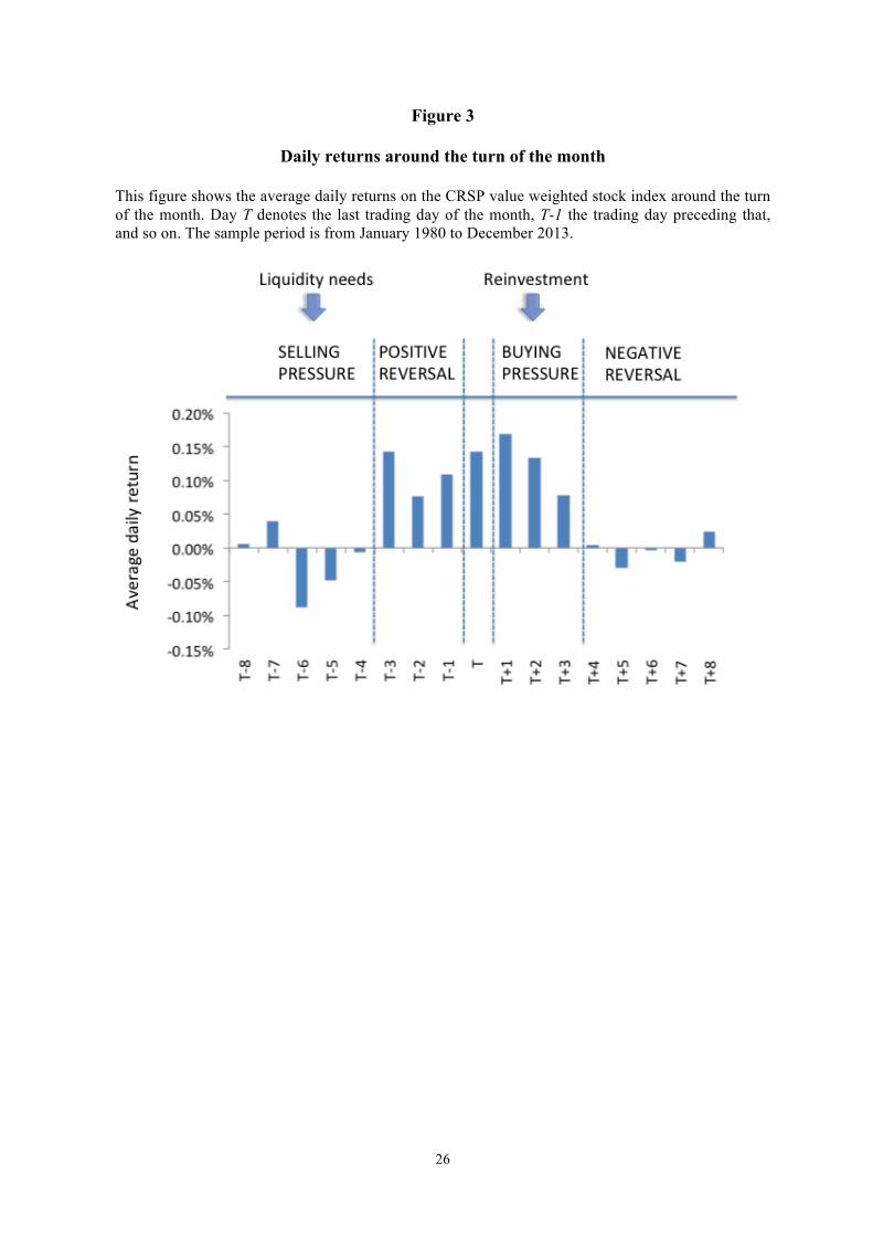
We illustrate some key events of our study in Figure 3 along with the daily average returns of the

CRSP value weighted stock index for each business day surrounding the month end. Consistent with

our understanding of the events, average returns are low from T-8 to T-4 (selling pressure) and high

from T-3 to T-1 (return reversal). As money begins to get reinvested in the market at the month end

and shortly after the month end, returns are again high from T to T+3 (buying pressure) and low

from T+4 to T+8 (return reversal). The differences in returns are economically meaningful: for

example, the average annualized S&P 500 return from T-8 to T-4 is -3.4% versus 28.6% from T-3 to

T+3.9

                                                                                                               9  Interestingly, the average excess returns that accrue to investors during the seven business days around the turn of the month cannot be explained by exposures to well-known risk factors: the CAPM alpha of the strategy is 5.6% per annum, the Fama and French (1993) three-factor alpha is 6.2% per annum; and the alpha with respect to a five-factor model that also includes the momentum factor of Carhart (1997) and the liquidity factor of Pastor and Stambaugh (2003) is 6.3% per annum. All alphas are statistically significant at the 1%

9

[INSERT FIGURE 3 HERE]

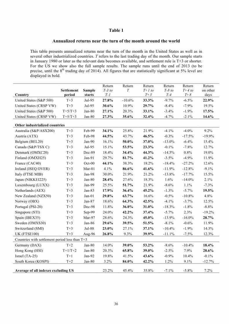
We can also observe similar return patterns in other developed markets, as displayed in Table 1,

which also reports the country-specific dates corresponding to the adoption of the 3-day (or shorter)

settlement rule. For all of the 24 markets in our sample, returns are statistically indistinguishable

from zero over the selling pressure period (T-8 to T-4) and positive and statistically significant over

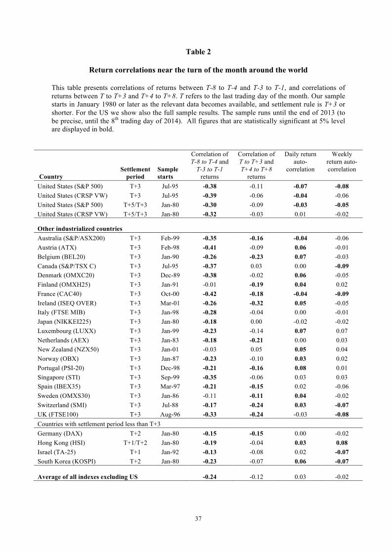
the reversal/buying pressure period from T-3 to T+3. Importantly, in Table 2 we establish a time-

series relationship between low returns over the selling pressure period of T-8 to T-4 and the returns

over the reversal period T-3 to T-1: in all of the 25 markets the correlations of returns between these

two periods’ returns are negative and in 22 of the 25 markets the correlations are statistically

significant. This evidence suggests that below-average returns over the selling pressure periods are

associated with above-average subsequent return reversals. Similarly, the time-series correlation

between the returns on days T to T+3 and the returns on the subsequent five days is either negative

and statistically significant (in 12 of the 25 markets) or insignificant. These negative correlations are

consistent with our hypothesis that there is first selling pressure and then buying pressure around the

turn of the month.10 11

[INSERT TABLE 1 AND 2 HERE]

4. Direct evidence from institutional investors’ trades To investigate the price pressure hypothesis as an explanation for the observed turn of the month

return patterns, we study a dataset that contains trade-level observations for hundreds of different

institutions (hedge funds, mutual funds, pension funds, and other money managers). Our data is from

Abel Noser Solutions (ANcerno) and it covers the period 1999-2013. This data includes the trades of

many of the largest institutional investors such as CalPERS, the YMCA retirement fund, Putman

Investments, and Lazard Asset Management (see Puckett and Yan, 2011). It has been used

extensively in recent academic research as it provides a highly representative sample of the

institutional fund management industry. According to Puckett and Yan, the institutions covered in

                                                                                                                                                                                                                                                                                                                                                     level. Results are qualitatively similar if instead of the CRSP value-weighted index we use the S&P 500 index in the alpha calculations. 10 The results for emerging markets are mixed. We regard this as evidence in favor of our hypothesis that the observed return reversals in developed markets are driven by efficient balance sheet management by institutional investors who are conscious of transaction costs and liquidity issues. We discuss these considerations in the next section. The unreported results for emerging markets are available from the authors. 11 The return patterns around T-3 documented in Tables 1 and 2 in the case of US stocks are robust to excluding from the sample the observations that coincide with year ends and quarter ends, observations that immediately precede the Fed’s announcements (that have been found to significantly impact average returns by Lucca and Moench, 2015) or observations overlapping with macro-economic announcement dates (that have been found to significantly impact average returns by Savor and Wilson, 2013).  

10

this dataset account for 8% of the daily volume in CRSP.

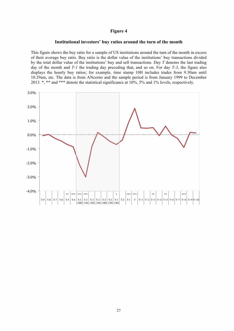
The ANcerno data reveals significant seasonalities in institutions’ buy-sell ratios. Consistent with our

hypothesis, the institutions in the sample seem to submit more sell than buy orders in the week that

precedes T-3, and more buy than sell orders in the days T-1 to T+4. On several days, such as T-5 to

T-3, T-1 to T, and T+3, the buy-sell ratios differ statistically significantly from the unconditional

mean. These daily average abnormal buy-sell ratios are displayed in Figure 4. For day T-3, the figure

also displays the hourly average abnormal ratios, allowing us to study the behavior of institutions

within the last day that guarantees cash settlement before the month end. Consistent with our

hypothesis, institutional selling pressure is strongest in the first hours of the trading day, and by early

afternoon, the institutions’ net buy ratios are indistinguishable from zero. Thus, by the end of the day

T-3, market prices will likely have started their recovery from liquidity-related institutional selling

pressures.

[INSERT FIGURE 4 HERE]

ANcerno’s trade-level data also allows us to estimate the costs incurred by institutions due to the

timing of their month-end trades. To do that, we compare the actual trading of these institutions to

hypothetical trading of equal volume with improved market timing by considering a scenario where

the institutions make at T all of the sales that they in reality made from T-5 to T-4. This calculation

suggests that, over the sample period 1999-2010, these institutions alone would have lost over 0.5

billion US dollars due to the timing of their trades. Assuming as in Puckett and Yan (2011) that the

institutions in ANcerno’s sample represent 10% of all institutional trading volume, the total cost of

month-end liquidity related trading to this type of institutions could be tenfold, 5 billion US dollars

during our sample period, or over 0.4 billion US dollars per year.12

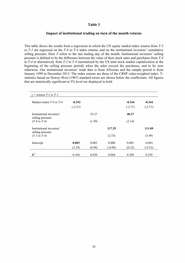
We can also use the ANcerno database for a regression-based study. The results in Table 3 show that

the cumulative net purchases of institutions during days T-5 to T-4 (normalized by the stock market

capitalization) negatively affect the stock market returns on days T-3 to T-1. This finding lends

additional direct support to our hypothesis that institutional trading generates predictable variation in

stock returns near the turn of the month.

[INSERT TABLE 3 HERE]

                                                                                                               12  If we include in these calculations the trades that happen in the morning of day T-3, the estimated total cost of month-end liquidity-related trading during our sample increases to 6 billion US dollars, or 0.5 billion US dollars per year.   Note   that   these   calculations   do   not   account   for   the   impact   of   potential   futures  transactions   that   would   enable   institutions   to   offset   the   reduction   in   their   market   exposures   at   the  month  end.    

11

In the next section, we will present further evidence on the role of institutions in the creation of turn

of the month return reversals by studying cross-sectional data on mutual fund holdings. We will also

investigate which types of stocks exhibit the strongest turn of the month reversals.

5. Cross-sectional evidence 5.1 Return reversals in the cross-section of stock returns

We begin our cross-sectional investigation with a straightforward extension of our aggregate stock

market study. Concretely, we sort the stocks in the CRSP universe each month based on their

performance over the period where we expect selling pressure, T-8 to T-4, and observe their average

returns over the subsequent three days where we expect reversals, T-3 to T-1, and over the

subsequent four days, T to T+3, which includes the days where we expect reinvestment-driven

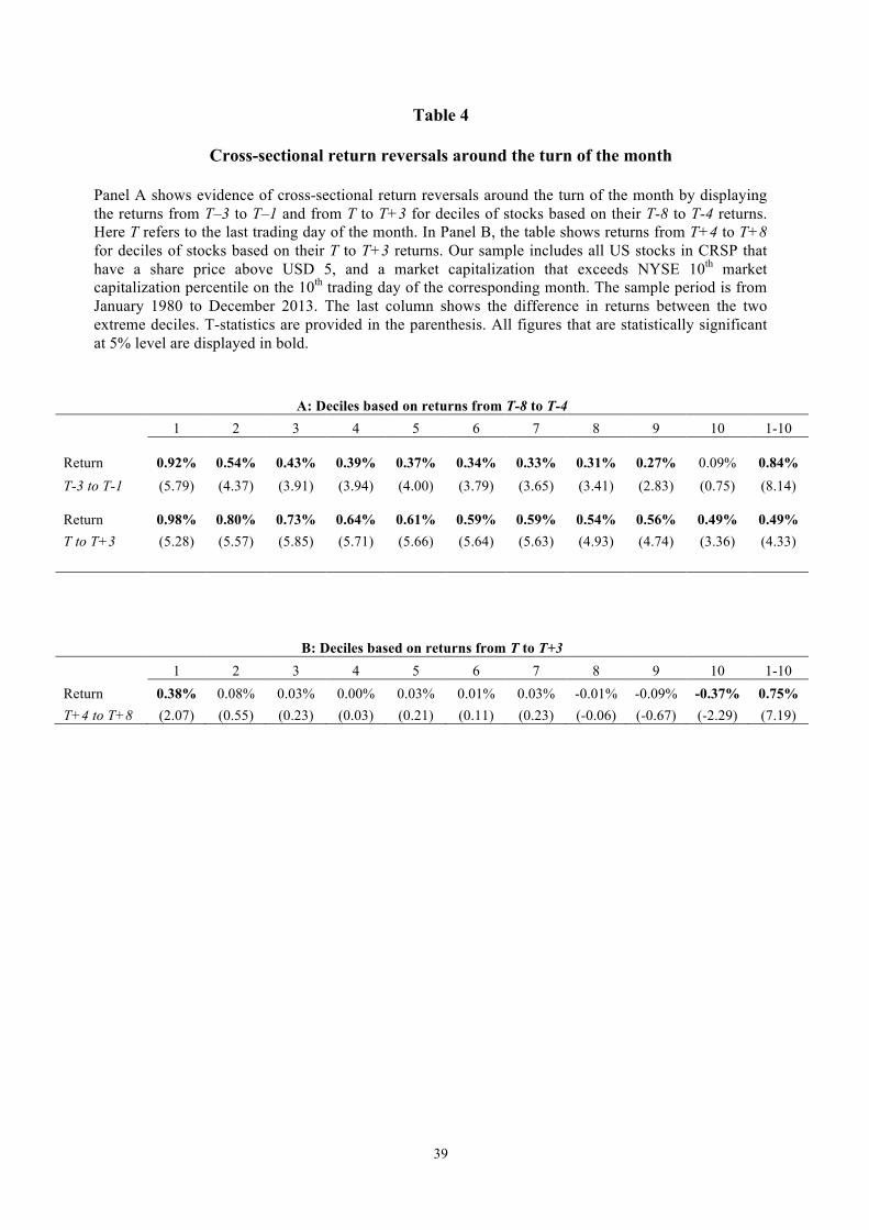
buying pressure. The results, displayed in Table 4, demonstrate that the worst-performing stocks

over the selling pressure period tend to exhibit best average performance over the subsequent three

and seven days. The relationship holds monotonically across our decile portfolios, formed based on

stocks’ each month's T-8 to T-4 returns. The difference in average returns between the lowest and

highest decile portfolios is both statistically and economically significant: 0.8% over the three-day

period T-3 to T-1, and 0.5% over the next four-day period T to T+3.13

[INSERT TABLE 4 HERE]

For completeness, we also conduct an analogous exercise for the period T+4 to T+8, where we

expect reversal from the beginning of the month buying pressure. The results, displayed in Panel B

of Table 4, demonstrate that the T+4 to T+8 average returns across the decile portfolios sorted on T

to T+3 returns also exhibit a large and statistically significant difference in average returns between

the extreme deciles.

We conclude that the month-end return patterns we observed for aggregate market indices also hold

for portfolios of individual stocks and the strength of return reversals is inversely proportional to the

stocks’ performance over the selling/buying pressure periods.

                                                                                                               13  We eliminate penny stocks and the smallest market capitalization stocks from our cross-sectional sample by requiring that the stock price is at least $5 and the stock’s market capitalization is above the 10th percentile of NYSE listed stocks on the 10th trading day of the corresponding month.  

12

5.2 Mutual fund ownership and turn of the month stock returns

We proposed that the return reversals in aggregate stock returns at the turn of the month are likely

driven by sales of stocks by institutional investors with month-end cash liabilities. If so, we would

expect the stocks owned in greater proportions by such investors to exhibit stronger return reversals.

While we do not directly observe the holdings of pension funds, whose payment obligations are

predominantly clustered at the month end (Figure 5A), we do observe the holdings of their agents,

mutual funds, which provide an easy and efficient implementation vehicle for pension funds’

diversified equity investments. 14 In addition to the payments of pension funds, the dividend

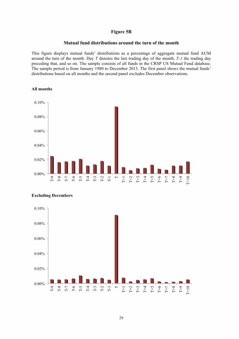
payments of mutual funds themselves also tend to cluster around the turn of the month (Figure 5B).15

Furthermore, the dividends of corporations received by mutual funds are also predominantly paid

around the turn of the month (Figure 5C). For all of these reasons, we suspect that the turn of the

month effects are more pronounced in the stocks that are commonly held by mutual funds.

[INSERT FIGURES 5A to 5C]

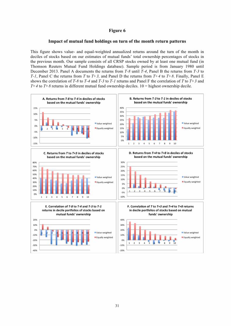
To investigate the link between mutual fund ownership and month-end return patterns, we sort the

US stocks in each month by mutual funds' collective ownership percentage in the previous month

and form decile portfolios. We then compute value-weighted average returns of these portfolios near

the turn of the month. The results are displayed in Figure 6. Consistent with our hypothesis, the

stocks that are held to a greater extent by mutual funds in a given month tend to experience

monotonically lower returns over the selling pressure period, from T-8 to T-4. These same stocks

also experience greater returns over the subsequent three days from T-3 to T-1, and again

monotonically lower average returns from T+4 to T+8. Finally, the correlation between T-8 to T-4

and T-3 to T-1 returns is more negative for those stocks that are more commonly held by mutual

funds.

[INSERT FIGURE 6 HERE]

In addition, the correlation between T to T+3 and T+4 to T+8 returns is negative only for the

portfolios of stocks in the six highest deciles of mutual fund ownership. All these pieces of evidence

suggest that mutual funds, and other institutions with month-end payment cycles, are a major force

behind the turn of the month phenomenon. It is therefore possible that the growth of the mutual fund

industry as a proportion of total stock market capitalization may have amplified the turn of the month

return patterns over time – a result that we document below.

                                                                                                               14 According to Investment Company Institute, approximately one half of US long-term mutual fund assets excluding money market funds are delegated by pension funds (http://www.ici.org/research/stats/retirement). 15 The only exception is the month of December where the dividend payments are more evenly distributed.

13

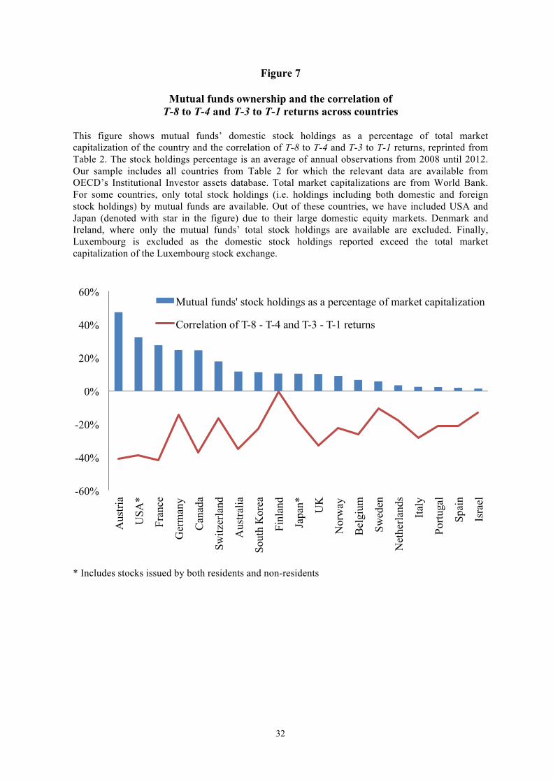
Before turning to the time series dimension, let us investigate the strength of month-end return

reversals across countries. Figure 7 displays the correlations of T-8 to T-4 returns and T-3 to T-1

returns for different equity indices across countries along with the percentage of the market

capitalization that is held by mutual funds within each country. It seems that the return reversals

around T-3 are indeed larger in countries where mutual funds are more prevalent. Using regression

analysis we confirm that this negative relationship between mutual fund ownership and the degree of

market return reversals around T-3 is statistically significant at the 1% level (results are available

upon request). The correlations presented in Figure 7 are negative for all country indexes.

[INSERT FIGURE 7 HERE]

Finally, we use regression analysis to study if there is a time-series relationship between the return

reversals around T-3 and the size of the US mutual fund industry. Our results, presented in Table 5,

show that the size of the mutual fund industry normalized by stock market capitalization is indeed

associated with the strength of market-wide return reversals around T-3: the interaction of the size of

the mutual fund industry with T-8 to T-4 returns is negative and statistically significant

[INSERT TABLE 5 HERE]

5.3. Other evidence that mutual funds affect turn of the month patterns

To further investigate the reasons why return patterns at the turn of the month may be related to

mutual fund ownership, we turn to the agency relationship between the mutual fund manager and the

end investor. Because of this agency relationship and a monthly reporting cycle, mutual fund

managers worried about sparking outflows might become less willing to take risk near the month

end. (see e.g. Sirri and Tufano, 1998). Month-end decreases in mutual fund risk appetite would not

only lead to additional selling pressure prior to T-3 but they would also explain why funds without

month-end liquidity needs might be unwilling to trade against liquidity-driven sellers near the month

end.

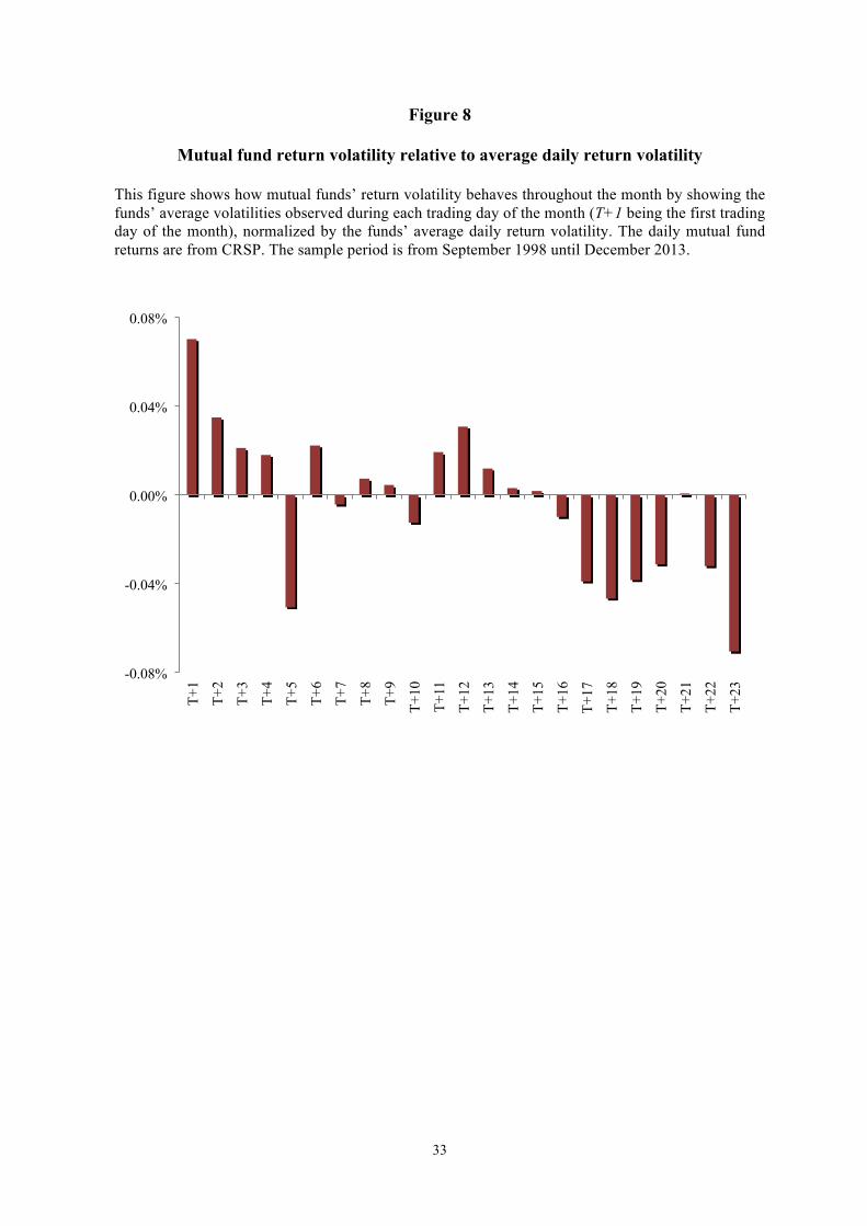
Our evidence presented in Table 6 and Figure 8 support this idea of month-end risk reduction. In

Table 6, we show that the average betas of mutual funds are abnormally low from T-5 to T-3. As

discussed, this result can arise from the average mutual fund’s need to sell assets prior to T-3 to meet

its month-end cash demands, or it can be a reflection of funds willingness to take less risk near the

end of the month. The finding in Figure 8 that mutual funds’ volatility decreases as the month goes

by can also be linked to either the average fund’s willingness to take less risk or its tendency to

14

accumulate cash to meet its payments near the month end. Irrespective of which one of these two

forces has a greater impact on funds’ behavior near the month end, such behavioral patterns can

contribute to the predictability of stock market returns around T-3 that we documented in Section 3.

[INSERT TABLE 6 AND FIGURE 8 HERE]

5.4 Stock characteristics and turn of the month returns

If the behavior of sophisticated investors is indeed inducing patterns in turn of the month stock

returns, these investors should at least be trying their best to avoid it. That is, any month-end

liquidity needs should be met with sales of liquid stocks, with minimal price impact and transaction

costs. To investigate this hypothesis, we sort the stocks in the CRSP universe based on different

characteristics that could be associated with transaction costs. The results are shown in Table 7.

[INSERT TABLE 7 HERE]

Consistent with the idea that mutual funds seek to meet their liquidity needs with minimal

transaction costs, we find that the correlation between T-8 to T-4 and T-3 to T-1 returns is most

negative for the most liquid, large cap stocks. Similarly, the return reversals around T+3 are only

negative for the largest and most liquid stocks.16

Furthermore, if the patterns we observe are in part due to mutual funds’ eagerness to reduce risk near

the month end, they should do so by reducing their holdings of risky but liquid stocks. We

investigate this idea in Table 8, which reports returns and correlations around the month end within

quartiles of stocks sorted by volatility, controlling for liquidity. Consistent with our intuition, we find

that return reversals around T-3 are most pronounced for the most volatile, yet liquid stocks.

[INSERT TABLE 8 HERE]

6. Hedge funds and funding constraints 6.1 Do hedge funds mitigate turn of the month return reversals?

In this section we investigate the behavior of hedge funds near the month end, looking for evidence

on their ability to mitigate the predictable patterns in market returns. Our evidence is mixed at best.

First, in Table 9, we show that the average market beta of hedge funds near the month end behaves

                                                                                                               16 For smaller and less liquid stocks, return correlations between T to T+3 and T+4 to T+8 are positive. This suggests that the institutions purchasing the least liquid stocks in the beginning of the month make their purchases gradually, continuing past the first three days of the month. Thus, again, they appear to operate conscious of transaction costs.

15

similarly to the average beta of mutual funds. This suggests that hedge funds do not provide liquidity

to mutual funds that sell near the month end, as one might have expected. In case of hedge funds, the

month-end patterns in betas may not only be related to the agency concerns regarding their own

monthly return reporting cycles, but also to the fact that their infrequent subscription and redemption

times are commonly set at month ends. This is likely to further increase their performance concerns

near the month end and potentially lead to a vigorous month-end cash cycle for hedge funds. Indeed,

we find some support for the latter reasoning as time-variation in betas seems to be more pronounced

for those funds with less frequent redemption periods (and presumably larger in- and outflows at

times of subscription and redemption). Therefore, it appears that the cash cycle and concerns related

to fund flows affect hedge funds’ ability and willingness to take risk near the month end – much in

the same way they seem to have reduced risk taking among mutual funds. 17

[INSERT TABLE 9 HERE]

If neither hedge funds nor mutual funds can or want to take risk near the month end, we would

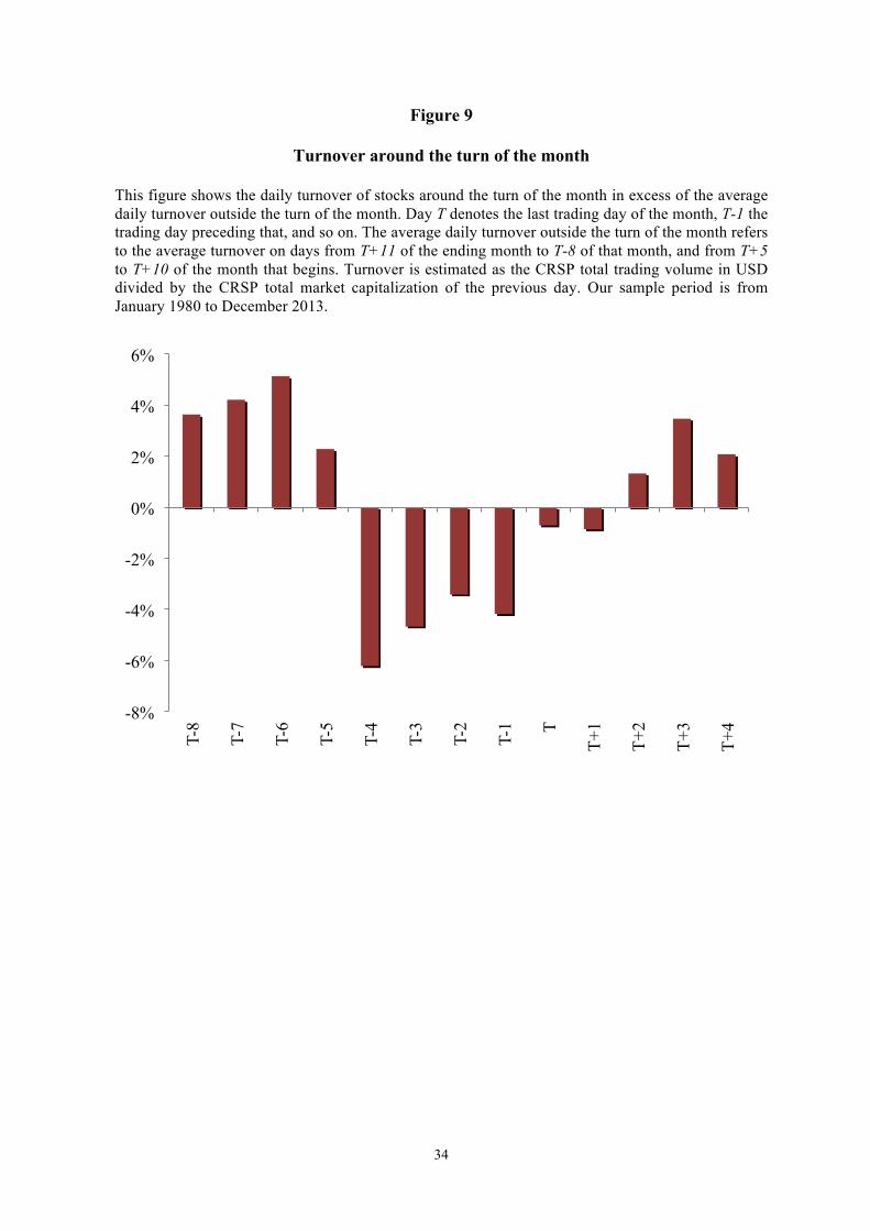
expect the stock market turnover to decrease also. We confirm this intuition in Figure 9, which

shows that trading volume is substantially lower than average during the last few trading days of the

month.18

[INSERT FIGURE 9 HERE]

While the hedge fund industry in aggregate does not seem to accommodate market-wide selling

pressure near the month end, it is possible that a subset of hedge funds do so. Indeed, we study the

behavior of different hedge fund strategies and find that Managed Futures and Global Macro funds

have abnormally large positive exposures to the market on day T-3 (see Table 10). This suggests that

at least some hedge funds do provide liquidity prior to T-3, counterbalancing the selling pressure

from other institutions. The evidence regarding liquidity supply is especially strong for Managed

Futures funds whose betas increase significantly on T-3.

[INSERT TABLE 10 HERE]

                                                                                                               17 Patton and Ramadorai (2013) study day-of-the-month effects in hedge fund risk exposures by including a flexible parametric function in their regression specification. Consistent with our results, they find that hedge fund risk exposures are high at the beginning of the month and low at the end of the month. 18 More detailed analysis reveals evidence that the drop in the trading volume between T-4 to T-1 is larger for the half of the stocks that are more commonly held by mutual funds.

16

6.2. Funding constraints and turn of the month returns

We find evidence that high levels of the TED spread are associated with amplified month-end return

reversals. This result is presented in Table 11, which shows that the interaction of TED spread with

T-8 to T-4 returns significantly predicts T-3 to T-1 returns. The finding lends support to the idea that

funding constraints of institutional investors are an important contributor to return reversals around

T-3: when short-term funding conditions are permissive (as proxied by low TED spread), institutions

need to rely less on selling and buying of stocks to manage their turn of the month liquidity needs.

The TED spread is perhaps most commonly used as a proxy for the funding liquidity of hedge funds

(e.g. Brunnermeier, Nagel and Pedersen, 2009). It is therefore conceivable that the TED spread

affects month-end return reversals primarily via hedge funds. To investigate this channel, we

consider a related variable, “hedge fund cost of leverage,” which we define as the TED spread

multiplied by aggregate hedge fund AUM (scaled by US stock market capitalization). We find that

the interaction of hedge fund cost of leverage and the return from T-8 to T-4 is a statistically

significant predictor of T-3 to T-1 returns, but only slightly more significant than the TED spread

interaction term alone. These findings provide evidence that low TED spread helps hedge funds (and

possibly other institutions as well) counterbalance month-end selling pressures with leverage. The

results are also reported in Table 11.

[INSERT TABLE 11 HERE]

7. Mutual fund alphas and exposure to month-end return reversals In this section, we present evidence that links mutual fund performance to fund-specific exposures to

month-end return reversals. Specifically, we sort mutual funds by the trailing two-year correlation of

their T-8 to T-4 and T-3 to T-1 returns and find that the funds in the highest correlation deciles have

significantly positive subsequent four-factor alphas, while the alphas for all of the other fund deciles

are negative or insignificant (see Figure 10 and Table 12). That is, funds that are less sensitive to

month-end return reversals – due to better month-end liquidity management practices or other

reasons – seem to be significantly more skilled than others. Exposure to market’s return reversals

predicts mutual fund performance.

[INSERT FIGURE 9 AND TABLE 12 HERE]

In Table 13, we seek to better understand this relationship by investigating the characteristics of

mutual funds within our correlation deciles. Consistent with our hypothesis that month-end liquidity

needs drive fund behavior, we find that the funds in the highest correlation decile have the highest

17

average cash holdings and may therefore depend less on stock sales to fulfill their month-end cash

needs. These funds also have the lowest institutional ownership share, suggesting that they are less

exposed to month end liquidity related selling in the first place. Finally, we find that the funds in the

highest correlation decile tend to generate higher returns not only during the turn of the month period

but also other days. That is, their outperformance cannot be fully attributed to their returns at the turn

of the month but they exhibit greater skill during the rest of the month also. Nonetheless, their rate of

outperformance is clearly higher during the last 8 trading days of the month.19 20

8. Conclusion In this paper, we attempt to provide a comprehensive analysis of month-end equity return patterns

and tie them to the literature on limits of arbitrage. We are the first to document a strong return

reversal around the most common last settlement day of the month, T-3, which guarantees cash for

month-end distributions. This return reversal exists in the time series of US stock index returns, in

the cross-section of US stock returns, and in the time series of most developed market stock index

returns. We argue that the reversal is driven mainly by the month-end cash cycle – which, as

previously argued by Ogden (1990), is also the likely cause of the abnormally high returns on the last

and the first three trading days of the month. The month-end cash cycle may therefore be the

unifying explanation for the exceptionally high returns observed during the seven days around the

turn of the month.

To shed some light on the underlying market dynamics, we present extensive evidence that links the

return reversals around T-3 to institutional investors’ trading, and their reduced willingness to take

risk near the month end. Our most direct evidence is based on ANcerno’s institutional trade data,

which reveals that institutions are on average net sellers prior to T-3, but net buyers at the end of the

month and on the first few days of the month. Indeed, we estimate that institutions may incur

significant costs from their liquidity-related trading at the month end. Moreover, using regression

analysis, we demonstrate that these institutions’ net sales on days T-8 to T-4 (normalized by the stock

                                                                                                               19  We  also  study  other fund characteristics often associated with performance (see e.g., Cremers and Petajisto, 2009) and find that the funds in our highest correlation decile are smallest by AUM, have the highest turnover and expense ratios, and the highest measured active shares (active share measures are described in Petajisto (2013) and are downloaded from http://www.petajisto.net). Motivated by Frazzini, Friedman and Pomorski (2015), we also find that the exposure to month-end reversals is linked to benchmark type: nearly 20% of small cap funds benchmarked to Russell 2000 are in the highest correlation decile while less than 4% of large cap funds benchmarked to Russell 1000 are in this decile.  20  A double sort based on the trailing two-year volatility of fund flows reveals that the differences across correlation deciles are larger for funds with higher flow volatility (the results are available from the authors upon request). In other unreported tests (also available from the authors), we find that the funds’ four-factor alphas rise linearly in their trailing two-year average returns measured over either T-8 to T-4 or T+4 to T+8. This additional finding suggests that sales prior to month end and purchases at the beginning of the month negatively impact fund alphas.    

18

market capitalization) significantly strengthens the market-wide return reversals at the month end. In

addition, we show that such turn of the month return reversals are more pronounced among stocks

that are more commonly held by mutual funds, and stocks that are arguably easier to use for cash

management, such as large and liquid stocks. Controlling for liquidity, we find that the reversals are

stronger for more volatile stocks, consistent with the idea that institutional investors seek to reduce

portfolio risk toward the month end for agency reasons. At an aggregate level, we show that the

return reversals near the turn of the month have only intensified as mutual funds’ AUM as a

proportion of the overall stock market has increased. Also in international samples, the return

reversals seem to be more pronounced in countries with larger mutual fund sectors. Finally, we

present evidence that mutual funds’ return patterns around the turn of the month (which presumably

reflect their liquidity management or other skills) significantly predict their future alphas.

Our results contribute to the literature by tying the vast body of existing research on turn of the

month return anomalies to rational models of markets with temporally segmented investors. In

addition, our findings have significant practical implications for institutions that currently

mismanage their turn of the month liquidity related trading.

19

References

Amihud, Y. “Illiquidity and Stock Returns: Cross-section and Time-series Effects.” Journal of

Financial Markets 5 (2002): 31-56.

Aragon, G. O. and Strahan P. E. (2012) Hedge funds as liquidity providers: evidence from Lehman

bankruptcy, Journal of Financial Economics 103, 570-587.

Ariel, R.A. "A monthly effect in stock returns." Journal of Financial Economics 18 (1987): 161-174.

Ben-Rephael, A., S. Kandel, and A. Wohl, “The price pressure of aggregate mutual fund flows.”

Journal of Financial and Quantitative Analysis 46 (2011): 585-603.

Brunnermeier, M., and L.H. Pedersen. “Market liquidity and funding liquidity.” Review of Financial

Studies 22 (2009): 2201-2238.

Brunnermeier, M., S. Nagel, and L.H. Pedersen. “Carry trades and currency crashes.” NBER

Macroeconomics Annual 2008 23 (2009): 313-347.

Cadsby, C. B., and R. Mitchell. "Turn-of-month and pre-holiday effects on stock returns: Some

international evidence." Journal of Banking & Finance 16 (1992): 497-509.

Campbell, J., S. Grossman, and J. Wang. “Trading volume and serial correlation in stock returns.”

Quarterly Journal of Economics 108 (1993): 905-939.

Carhart, M. “On persistence in mutual fund performance.” Journal of Finance 52 (1997): 57-82.

Cremers, M and A. Petajisto. “How Active Is Your Fund Manager? A New Measure that Predicts

Performance.” Review of Financial Studies 22 (2009): 3329-3365.

Duffie, D. “Presidential Address: Asset Price Dynamics with Slow-moving Capital.” Journal of

Finance 65 (2010): 1237-1267.

Dzhabarov, C., and W. T. Ziemba. "Do seasonal anomalies still work?" The Journal of Portfolio

Management 36 (2010): 93-104.

20

Fama, E., and K. French. “The cross-section of expected stock returns.” Journal of Finance 47

(1992): 427-465.

Frazzini, A., J.A. Friedman, and L. Pomorski. “Deactivating Active Share.” AQR Working Paper

(2015).

Gromb, D., and D. Vayanos. “Limits of arbitrage: the state of the theory.” Annual Review of

Financial Economics 2 (2012): 251-275.

Grossman, S., and M. Miller. “Liquidity and market structure.” Journal of Finance 43(1988): 617-

633.

Henderson, B.J., N.D. Pearson, and L. Wang. “New Evidence on the Financialization of Commodity

Markets.” Review of Financial Studies 28 (2015): 1285-1311.

Jylhä, P., and M. Suominen. “Speculative capital and currency carry trades.” Journal of Financial

Economics 99 (2011): 60–75.

Lakonishok, J., A. Shleifer, R. Thaler, and R. W. Vishny. “Window dressing by pension fund

managers.” American Economic Review 81 (1991): 227–231.

Lakonishok, J., and S. Smidt. "Are seasonal anomalies real? A ninety-year perspective." Review of

Financial Studies 1 (1988): 403-425.

Lou, D., H. Yan, and J. Zhang. “Anticipated and Repeated Shocks in Liquid Markets.” Review of

Financial Studies 26 (2013): 1891-1912.

Lucca, D., and E. Moench. “The Pre-FOMC announcement drift.“ Journal of Finance 70 (2015):

329–371.

McConnell, J. J., and W. Xu. "Equity returns at the turn of the month." Financial Analysts Journal

64 (2008): 49-64.

Mou, Y. “Limits to arbitrage and commodity index investment: front-running the Goldman Roll.”

Working Paper, Columbia University (2011).

21

Newey, W. K. and K. D. West, "A Simple, Positive Semi-definite, Heteroskedasticity and

Autocorrelation Consistent Covariance Matrix." Econometrica 55 (1987): 703–708

Ogden, J. P. "Turn‐of‐month evaluations of liquid profits and stock returns: a common explanation

for the monthly and January Effects." The Journal of Finance 45 (1990): 1259-1272.

Pastor, L., and R. Stambaugh. “Liquidity risk and expected stock returns.” Journal of Political

Economy 111 (2003): 642-685.

Patton, A., and T. Ramadorai. “On the high-frequency dynamics of hedge fund risk exposures.”

Journal of Finance 68 (2013): 597–635.

Petajisto, A. “Active share and mutual fund performance.” Financial Analysts Journal 69 (2013):

73-93.

Puckett, A., and X. Yan. “The interim trading skills of institutional investors.” Journal of Finance 66

(2011):601–633.

Savor, P. and M. Wilson. “How much do investors care about macroeconomic risk? Evidence from

scheduled economic announcements.” Journal of Financial and Quantitative Analysis 48 (2013):

343 – 375.

Sirri, E., and P. Tufano. “Costly search and mutual fund flows.” Journal of Finance 53 (1998):1589–

1622.

22

Figure 1

Cumulative returns around the turn of the month

This figure shows the cumulative excess returns (Rm-Rf) from investing in the CRSP value weighted total return stock index only on days T-3 to T+3 around the turn of the month, where T refers to the last day of the month, T+3 to the third business day of the month, and so on. It shows also the returns from investing in the same index only on days T-8 to T-4, only on days T+4 to T+8, and only on days outside T-8 to T+8. The sample period is from July 1926 to December 2013. Note logarithmic scale.

0.01

0.1

1

10

100

1000

1926

19

29

1932

19

35

1938

19

41

1944

19

47

1950

19

53

1956

19

59

1962

19

65

1968

19

71

1974

19

77

1980

19

83

1986

19

89

1992

19

95

1998

20

01

2004

20

07

2010

20

13

From T-3 to T+3 From T-8 to T-4 From T+4 to T+8 On other days

23

Figure 2A

Deposits around the turn of the month

This figure shows the deposits in US Commercial banks relative to their two month average surrounding the observation date, on various trading days around the turn of the month. T is the last day of the month. The sample period is from January 1980 to December 2013. Source: FRED database.

0.985

0.990

0.995

1.000

1.005

1.010

1.015

T-9

T-8

T-7

T-6

T-5

T-4

T-3

T-2

T-1 T

T+1

T+2

T+3

T+4

T+5

T+6

T+7

T+8

T+9

T+10

24

Figure 2B

Federal Funds rate around the turn of the month

This figure shows the level of effective Federal Funds rate excess of its monthly average around the turn of the month. Day T denotes the last trading day of the month and T-1 the trading day preceding that, and so on. The data is from Federal Reserve. The sample period is from January 1980 to December 2013. *, ** and *** denote statistical significance at 10%, 5% and 1% levels, respectively.

-0.10%

-0.05%

0.00%

0.05%

0.10%

0.15%

0.20%

T-9

T-8

T-7

T-6

T-5

T-4

T-3

T-2

T-1 T

T+1

T+2

T+3

T+4

T+5

T+6

T+7

T+8

T+9

T+10

- - - - *** *** *** * - *** *** *** - * ** *** *** *** ** -

25

Figure 2C

Libor rate around the turn of the month

This figure shows the level of Libor rate (USD overnight) excess of its monthly average around the turn of the month. Day T denotes the last trading day of the month, T-1 the trading day preceding that, and so on. The data is from Federal Reserve. The sample period is from January 2001 to December 2013. *, ** and *** denote statistical significance at 10%, 5% and 1% levels, respectively.

-0.06%

-0.04%

-0.02%

0.00%

0.02%

0.04%

0.06%

0.08%

0.10%

T-9

T-8

T-7

T-6

T-5

T-4

T-3

T-2

T-1 T

T+1

T+2

T+3

T+4

T+5

T+6

T+7

T+8

T+9

T+10

- - *** *** *** *** *** - - *** *** ** - - - - - * ** -

26

Figure 3

Daily returns around the turn of the month This figure shows the average daily returns on the CRSP value weighted stock index around the turn of the month. Day T denotes the last trading day of the month, T-1 the trading day preceding that, and so on. The sample period is from January 1980 to December 2013.

27

Figure 4

Institutional investors’ buy ratios around the turn of the month This figure shows the buy ratio for a sample of US institutions around the turn of the month in excess of their average buy ratio. Buy ratio is the dollar value of the institutions’ buy transactions divided by the total dollar value of the institutions’ buy and sell transactions. Day T denotes the last trading day of the month and T-1 the trading day preceding that, and so on. For day T-3, the figure also displays the hourly buy ratios; for example, time stamp 10H includes trades from 9.30am until 10.29am, etc. The data is from ANcerno and the sample period is from January 1999 to December 2013. *, ** and *** denote the statistical significance at 10%, 5% and 1% levels, respectively.

-­‐4.0%  

-­‐3.0%  

-­‐2.0%  

-­‐1.0%  

0.0%  

1.0%  

2.0%  

3.0%  

** *** *** *** * *** *** ** ** ***

T-9 T-8 T-7 T-6 T-5 T-4 T-3 10H

T-3 11H

T-3 12H

T-3 13H

T-3 14H

T-3 15H

T-3 16H

T-2 T-1 T T+1 T+2 T+3 T+4 T+5 T+6 T+7 T+8 T+9 T+10

28

Figure 5A

Pension fund payment dates around the turn of the month

This figure shows the proportion of pension payment dates around the turn of the month. Day T denotes the last trading day of the month, T-1 the trading day preceding that, and so on. The data, obtained from Pension & Investment 300 Analysis (2012) by Tower Watson and individual pension fund websites, include 15 of the 19 largest US public pension plans.

0%

10%

20%

30%

40%

50%

T-9

T-8

T-7

T-6

T-5

T-4

T-3

T-2

T-1 T

T+1

T+2

T+3

T+4

T+5

T+6

T+7

T+8

T+9

T+10

29

Figure 5B

Mutual fund distributions around the turn of the month This figure displays mutual funds’ distributions as a percentage of aggregate mutual fund AUM around the turn of the month. Day T denotes the last trading day of the month, T-1 the trading day preceding that, and so on. The sample consists of all funds in the CRSP US Mutual Fund database. The sample period is from January 1980 to December 2013. The first panel shows the mutual funds’ distributions based on all months and the second panel excludes December observations. All months

Excluding Decembers

0.00%

0.02%

0.04%

0.06%

0.08%

0.10%

T-9

T-8

T-7

T-6

T-5

T-4

T-3

T-2

T-1 T

T+1

T+2

T+3

T+4

T+5

T+6

T+7

T+8

T+9

T+10

0.00%

0.02%

0.04%

0.06%

0.08%

0.10%

T-9

T-8

T-7

T-6

T-5

T-4

T-3

T-2

T-1 T

T+1

T+2

T+3

T+4

T+5

T+6

T+7

T+8

T+9

T+10

30

Figure 5C

Corporate dividend payment dates around the turn of the month

The figure shows the proportion of annual dividend payments (in dollars) by CRSP companies occurring around the turn of the month. Day T denotes the last trading day of the month, T-1 the trading day preceding that, and so on. The sample period is from January 1980 to December 2013.

0%

5%

10%

15%

20%

25%

T-9

T-8

T-7

T-6

T-5

T-4

T-3

T-2

T-1 T

T+1

T+2

T+3

T+4

T+5

T+6

T+7

T+8

T+9

T+10

31

Figure 6

Impact of mutual fund holdings on turn of the month return patterns This figure shows value- and equal-weighted annualized returns around the turn of the month in deciles of stocks based on our estimates of mutual funds’ total ownership percentages of stocks in the previous month. Our sample consists of all CRSP stocks owned by at least one mutual fund (in Thomson Reuters Mutual Fund Holdings database). Sample period is from January 1980 until December 2013. Panel A documents the returns from T-8 until T-4, Panel B the returns from T-3 to T-1, Panel C the returns from T to T+3, and Panel D the returns from T+4 to T+8. Finally, Panel E shows the correlation of T-8 to T-4 and T-3 to T-1 returns and Panel F the correlation of T to T+3 and T+4 to T+8 returns in different mutual fund ownership deciles. 10 = highest ownership decile.

32

Figure 7

Mutual funds ownership and the correlation of T-8 to T-4 and T-3 to T-1 returns across countries

This figure shows mutual funds’ domestic stock holdings as a percentage of total market capitalization of the country and the correlation of T-8 to T-4 and T-3 to T-1 returns, reprinted from Table 2. The stock holdings percentage is an average of annual observations from 2008 until 2012. Our sample includes all countries from Table 2 for which the relevant data are available from OECD’s Institutional Investor assets database. Total market capitalizations are from World Bank. For some countries, only total stock holdings (i.e. holdings including both domestic and foreign stock holdings) by mutual funds are available. Out of these countries, we have included USA and Japan (denoted with star in the figure) due to their large domestic equity markets. Denmark and Ireland, where only the mutual funds’ total stock holdings are available are excluded. Finally, Luxembourg is excluded as the domestic stock holdings reported exceed the total market capitalization of the Luxembourg stock exchange.

* Includes stocks issued by both residents and non-residents

-60%

-40%

-20%

0%

20%

40%

60%

Aus

tria

USA

*

Fran

ce

Ger

man

y

Can

ada

Switz

erla

nd

Aus

tralia

Sout

h K

orea

Finl

and

Japa

n*

UK

Nor

way

Bel

gium

Swed

en

Net

herla

nds

Italy

Portu

gal

Spai

n

Isra

el

Mutual funds' stock holdings as a percentage of market capitalization

Correlation of T-8 - T-4 and T-3 - T-1 returns

33

Figure 8

Mutual fund return volatility relative to average daily return volatility

This figure shows how mutual funds’ return volatility behaves throughout the month by showing the funds’ average volatilities observed during each trading day of the month (T+1 being the first trading day of the month), normalized by the funds’ average daily return volatility. The daily mutual fund returns are from CRSP. The sample period is from September 1998 until December 2013.

-0.08%

-0.04%

0.00%

0.04%

0.08%

T+1

T+2

T+3

T+4

T+5

T+6

T+7

T+8

T+9

T+10

T+11

T+12

T+13

T+14

T+15

T+16

T+17

T+18

T+19

T+20

T+21

T+22

T+23

34

Figure 9

Turnover around the turn of the month

This figure shows the daily turnover of stocks around the turn of the month in excess of the average daily turnover outside the turn of the month. Day T denotes the last trading day of the month, T-1 the trading day preceding that, and so on. The average daily turnover outside the turn of the month refers to the average turnover on days from T+11 of the ending month to T-8 of that month, and from T+5 to T+10 of the month that begins. Turnover is estimated as the CRSP total trading volume in USD divided by the CRSP total market capitalization of the previous day. Our sample period is from January 1980 to December 2013.

-8%

-6%

-4%

-2%

0%

2%

4%

6%

T-8

T-7

T-6

T-5

T-4

T-3

T-2

T-1 T

T+1

T+2

T+3

T+4

35

Figure 10

Exposure to month-end return reversals predicts mutual fund performance

This figure shows mutual funds’ four factor alphas conditional on fund-specific trailing two-year correlations between the funds’ T-8 to T-4 and T-3 to T-1 returns. More specifically, funds are divided into deciles every year (at the end of December) based on this correlation. Four factor alphas are calculated using the subsequent year’s daily returns controlling for the three factors of Fama and French and Carhart’s Momentum factor. Decile 10 contains the funds with the highest correlation in their T-8 to T-4 and T-3 to T-1 returns. The daily mutual fund returns are from CRSP. The sample period is from January 1999 to December 2013.

 

-3.0%

-2.0%

-1.0%

0.0%

1.0%

2.0%

3.0%

4.0%

1 2 3 4 5 6 7 8 9 10

Equal-weighted average of fund-specific alphas

Alpha of equal-weighted mutual fund portfolios

36

Table 1

Annualized returns near the turn of the month around the world

This table presents annualized returns near the turn of the month in the United States as well as in several other industrialized countries. T refers to the last trading day of the month. Our sample starts in January 1980 or later as the relevant data becomes available, and settlement rule is T+3 or shorter. For the US we show also the full sample results. The sample runs until the end of 2013 (to be precise, until the 8th trading day of 2014). All figures that are statistically significant at 5% level are displayed in bold.

Country Settlement

period

Sample starts

Return T-3 to

T-1

Return T

Return T+1 to

T+3

Return T-8 to

T-4

Return T+4 to

T+8

Return on other

days United States (S&P 500) T+3 Jul-95 27.8% -10.6% 33.3% -9.7% -6.5% 22.9% United States (CRSP VW) T+3 Jul-95 30.6% 10.9% 29.7% -8.4% -7.9% 19.5% United States (S&P 500) T+5/T+3 Jan-80 27.1% 20.3% 33.1% -3.4% -1.9% 17.5% United States (CRSP VW) T+5/T+3 Jan-80 27.3% 35.6% 32.4% -4.7% -2.1% 14.6%

Other industrialized countries Australia (S&P/ASX200) T+3 Feb-99 34.1% 25.8% 21.9% -4.1% -4.0% 9.2% Austria (ATX) T+3 Feb-98 44.5% 43.7% 46.5% -0.3% -17.5% -19.9% Belgium (BEL20) T+3 Jan-90 16.1% 50.0% 37.0% -13.0% -6.4% 15.4% Canada (S&P/TSX C) T+3 Jul-95 15.1% 53.5% 23.3% -0.1% -7.8% 12.7% Denmark (OMXC20) T+3 Dec-89 18.4% 34.4% 44.3% -14.5% 0.8% 19.0% Finland (OMXH25) T+3 Jan-91 29.7% 81.7% 41.2% -3.5% -4.9% 11.9% France (CAC40) T+3 Oct-00 44.1% 38.3% 18.2% -18.4% -27.2% 12.6% Ireland (ISEQ OVER) T+3 Mar-01 4.1% 86.6% 41.6% -11.9% -12.8% -9.1% Italy (FTSE MIB) T+3 Jan-98 30.0% 21.9% 21.2% -13.8% -17.7% 15.5% Japan (NIKKEI225) T+3 Jan-80 28.4% 27.6% 18.3% 1.6% -14.0% 2.1% Luxembourg (LUXX) T+3 Jan-99 25.5% 51.7% 21.9% -8.6% 1.1% -7.3% Netherlands (AEX) T+3 Jan-83 17.9% 36.4% 45.2% -1.3% -5.7% 19.5% New Zealand (NZX50) T+3 Jan-01 29.8% 63.7% 16.6% -0.5% -10.8% 4.8% Norway (OBX) T+3 Jan-87 18.6% 64.3% 42.5% -4.1% -3.7% 12.5% Portugal (PSI-20) T+3 Dec-98 11.8% 36.0% 31.0% -18.3% -1.8% -8.8% Singapore (STI) T+3 Sep-99 24.0% 42.2% 37.4% -5.7% 2.3% -19.2% Spain (IBEX35) T+3 Mar-97 28.6% 24.3% 45.0% -13.9% -16.0% 28.7% Sweden (OMXS30) T+3 Jan-86 29.6% 39.5% 51.5% -8.1% -0.6% 11.9% Switzerland (SMI) T+3 Jul-88 23.0% 27.1% 37.1% -10.4% -1.9% 14.3% UK (FTSE100) T+3 Aug-96 26.8% 9.3% 39.9% -11.1% -7.5% 12.3% Countries with settlement period less than T+3 Germany (DAX) T+2 Jan-80 14.0% 39.0% 53.2% -8.6% -10.4% 18.4% Hong Kong (HSI) T+1/T+2 Jan-80 20.3% 65.8% 39.0% -2.5% 7.9% 28.6% Israel (TA-25) T+1 Jan-92 19.8% 41.5% 43.6% -0.9% 10.4% -0.1% South Korea (KOSPI) T+2 Jan-80 3.2% 84.0% 42.2% 1.2% 9.1% -12.7% Average of all indexes excluding US 23.2% 45.4% 35.8% -7.1% -5.8% 7.2%

37

Table 2

Return correlations near the turn of the month around the world

This table presents correlations of returns between T-8 to T-4 and T-3 to T-1, and correlations of returns between T to T+3 and T+4 to T+8. T refers to the last trading day of the month. Our sample starts in January 1980 or later as the relevant data becomes available, and settlement rule is T+3 or shorter. For the US we show also the full sample results. The sample runs until the end of 2013 (to be precise, until the 8th trading day of 2014). All figures that are statistically significant at 5% level are displayed in bold.

Country Settlement

period Sample starts

Correlation of T-8 to T-4 and

T-3 to T-1 returns

Correlation of T to T+3 and T+4 to T+8

returns

Daily return auto-

correlation

Weekly return auto- correlation

United States (S&P 500) T+3 Jul-95 -0.38 -0.11 -0.07 -0.08 United States (CRSP VW) T+3 Jul-95 -0.39 -0.06 -0.04 -0.06 United States (S&P 500) T+5/T+3 Jan-80 -0.30 -0.09 -0.03 -0.05 United States (CRSP VW) T+5/T+3 Jan-80 -0.32 -0.03 0.01 -0.02

Other industrialized countries

Australia (S&P/ASX200) T+3 Feb-99 -0.35 -0.16 -0.04 -0.06 Austria (ATX) T+3 Feb-98 -0.41 -0.09 0.06 -0.01 Belgium (BEL20) T+3 Jan-90 -0.26 -0.23 0.07 -0.03 Canada (S&P/TSX C) T+3 Jul-95 -0.37 0.03 0.00 -0.09 Denmark (OMXC20) T+3 Dec-89 -0.38 -0.02 0.06 -0.05 Finland (OMXH25) T+3 Jan-91 -0.01 -0.19 0.04 0.02 France (CAC40) T+3 Oct-00 -0.42 -0.18 -0.04 -0.09 Ireland (ISEQ OVER) T+3 Mar-01 -0.26 -0.32 0.05 -0.05 Italy (FTSE MIB) T+3 Jan-98 -0.28 -0.04 0.00 -0.01 Japan (NIKKEI225) T+3 Jan-80 -0.18 0.00 -0.02 -0.02 Luxembourg (LUXX) T+3 Jan-99 -0.23 -0.14 0.07 0.07 Netherlands (AEX) T+3 Jan-83 -0.18 -0.21 0.00 0.03 New Zealand (NZX50) T+3 Jan-01 -0.03 0.05 0.05 0.04 Norway (OBX) T+3 Jan-87 -0.23 -0.10 0.03 0.02 Portugal (PSI-20) T+3 Dec-98 -0.21 -0.16 0.08 0.01 Singapore (STI) T+3 Sep-99 -0.35 -0.06 0.03 0.03 Spain (IBEX35) T+3 Mar-97 -0.21 -0.15 0.02 -0.06 Sweden (OMXS30) T+3 Jan-86 -0.11 -0.11 0.04 -0.02 Switzerland (SMI) T+3 Jul-88 -0.17 -0.24 0.03 -0.07 UK (FTSE100) T+3 Aug-96 -0.33 -0.24 -0.03 -0.08 Countries with settlement period less than T+3 Germany (DAX) T+2 Jan-80 -0.15 -0.15 0.00 -0.02 Hong Kong (HSI) T+1/T+2 Jan-80 -0.19 -0.04 0.03 0.08 Israel (TA-25) T+1 Jan-92 -0.13 -0.08 0.02 -0.07 South Korea (KOSPI) T+2 Jan-80 -0.23 -0.07 0.06 -0.07 Average of all indexes excluding US -0.24 -0.12 0.03 -0.02

38

Table 3

Impact of institutional trading on turn of the month returns

This table shows the results from a regression in which the US equity market index returns from T-3 to T-1 are regressed on the T-8 to T-4 index returns, and on the institutional investors’ cumulative selling pressure. Here T refers to the last trading day of the month. Institutional investors’ selling pressure is defined to be the difference between the value of their stock sales and purchases from T-8 to T-4 or alternatively from T-5 to T-4 (normalized by the US total stock market capitalization at the beginning of the selling pressure period) when the sales exceed the purchases, and to be zero otherwise. Our institutional investors’ trade data is from ANcerno and the sample period is from January 1999 to December 2013. The index returns are those of the CRSP value-weighted index. T-statistics based on Newey-West (1987) standard errors are shown below the coefficients. All figures that are statistically significant at 5% level are displayed in bold.

y = returns T-3 to T-1

Market return T-8 to T-4 -0.352

-0.344 -0.344

(-2.51) (-2.71) (-2.71) Institutional investors’ 35.27 40.37 selling pressure (T-8 to T-4) (1.50) (2.14) Institutional investors’ 117.25 111.09 selling pressure (T-5 to T-4) (2.53) (3.49)

Intercept 0.003 0.002 0.000 0.001 -0.001 (2.39) (0.98) (-0.09) (0.32) (-0.52)

R2 0.184 0.020 0.084 0.209 0.259

39

Table 4

Cross-sectional return reversals around the turn of the month

Panel A shows evidence of cross-sectional return reversals around the turn of the month by displaying the returns from T–3 to T–1 and from T to T+3 for deciles of stocks based on their T-8 to T-4 returns. Here T refers to the last trading day of the month. In Panel B, the table shows returns from T+4 to T+8 for deciles of stocks based on their T to T+3 returns. Our sample includes all US stocks in CRSP that have a share price above USD 5, and a market capitalization that exceeds NYSE 10th market capitalization percentile on the 10th trading day of the corresponding month. The sample period is from January 1980 to December 2013. The last column shows the difference in returns between the two extreme deciles. T-statistics are provided in the parenthesis. All figures that are statistically significant at 5% level are displayed in bold.

A: Deciles based on returns from T-8 to T-4

1 2 3 4 5 6 7 8 9 10 1-10

Return 0.92% 0.54% 0.43% 0.39% 0.37% 0.34% 0.33% 0.31% 0.27% 0.09% 0.84% T-3 to T-1 (5.79) (4.37) (3.91) (3.94) (4.00) (3.79) (3.65) (3.41) (2.83) (0.75) (8.14) Return 0.98% 0.80% 0.73% 0.64% 0.61% 0.59% 0.59% 0.54% 0.56% 0.49% 0.49% T to T+3 (5.28) (5.57) (5.85) (5.71) (5.66) (5.64) (5.63) (4.93) (4.74) (3.36) (4.33)

B: Deciles based on returns from T to T+3

1 2 3 4 5 6 7 8 9 10 1-10

Return 0.38% 0.08% 0.03% 0.00% 0.03% 0.01% 0.03% -0.01% -0.09% -0.37% 0.75% T+4 to T+8 (2.07) (0.55) (0.23) (0.03) (0.21) (0.11) (0.23) (-0.06) (-0.67) (-2.29) (7.19)

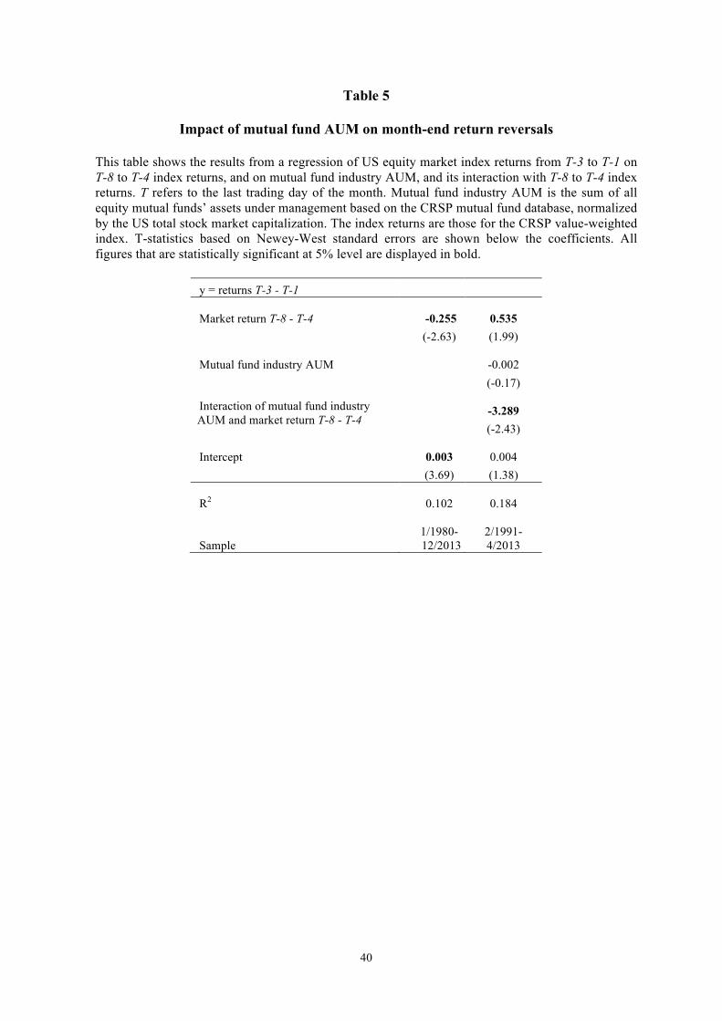
40

Table 5

Impact of mutual fund AUM on month-end return reversals

This table shows the results from a regression of US equity market index returns from T-3 to T-1 on T-8 to T-4 index returns, and on mutual fund industry AUM, and its interaction with T-8 to T-4 index returns. T refers to the last trading day of the month. Mutual fund industry AUM is the sum of all equity mutual funds’ assets under management based on the CRSP mutual fund database, normalized by the US total stock market capitalization. The index returns are those for the CRSP value-weighted index. T-statistics based on Newey-West standard errors are shown below the coefficients. All figures that are statistically significant at 5% level are displayed in bold.

y = returns T-3 - T-1

Market return T-8 - T-4 -0.255 0.535 (-2.63) (1.99)

Mutual fund industry AUM -0.002 (-0.17)

Interaction of mutual fund industry AUM and market return T-8 - T-4

-3.289 (-2.43)

Intercept 0.003 0.004 (3.69) (1.38)

R2 0.102 0.184

Sample 1/1980-12/2013

2/1991-4/2013

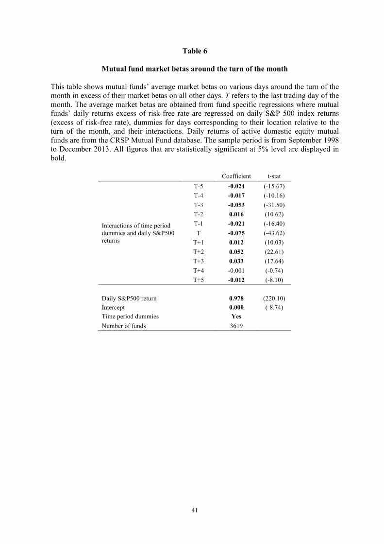
41

Table 6

Mutual fund market betas around the turn of the month

This table shows mutual funds’ average market betas on various days around the turn of the month in excess of their market betas on all other days. T refers to the last trading day of the month. The average market betas are obtained from fund specific regressions where mutual funds’ daily returns excess of risk-free rate are regressed on daily S&P 500 index returns (excess of risk-free rate), dummies for days corresponding to their location relative to the turn of the month, and their interactions. Daily returns of active domestic equity mutual funds are from the CRSP Mutual Fund database. The sample period is from September 1998 to December 2013. All figures that are statistically significant at 5% level are displayed in bold.

Coefficient t-stat

Interactions of time period dummies and daily S&P500 returns

T-5 -0.024 (-15.67) T-4 -0.017 (-10.16) T-3 -0.053 (-31.50) T-2 0.016 (10.62) T-1 -0.021 (-16.40) T -0.075 (-43.62)

T+1 0.012 (10.03) T+2 0.052 (22.61) T+3 0.033 (17.64) T+4 -0.001 (-0.74) T+5 -0.012 (-8.10)

Daily S&P500 return 0.978 (220.10) Intercept 0.000 (-8.74) Time period dummies Yes Number of funds 3619

42

Table 7

Stock-level liquidity, size and turn of the month patterns

A. This table shows the impact of stock-level liquidity on turn of the month return patterns. Our sample, covering data from January 1980 to December 2013, includes all stocks in CRSP listed in the NYSE and the Amex, that have share price above USD 5 on the 10th trading day of corresponding month and a market capitalization that exceeds the NYSE 10th market capitalization percentile. Amihud (2002) ILLIQ measure is calculated as a rolling one year average until the 10th trading day of corresponding month. For stocks sorted into deciles based on their Amihud measure (10th being the most illiquid), the table shows the annualized value-weighted returns on the relevant dates, and the correlations between T-8 to T-4 and T-3 to T-1 returns and T to T+3 and T+4 to T+8 returns, respectively. T refers to the last trading day of the month. All figures that are statistically significant at 5% level are displayed in bold.

Amihud Decile

Annualized return

T-3 - T-1

Annualized return

T

Annualized return

T+1 - T+3

Annualized return

T-8 - T-4

Annualized return

T+4 - T+8

Annualized return on

other days

Correlation of T-8 - T-4 and

T-3 - T-1 returns

Correlation of T - T+3 and T+4 - T+8

returns

1 27.5% 13.4% 31.6% -3.9% -1.3% 17.1% -0.29 -0.10

2 32.4% 46.2% 32.4% -5.4% -3.3% 16.0% -0.29 -0.04

3 34.8% 53.6% 35.1% -8.2% -3.0% 18.2% -0.29 -0.03

4 35.2% 60.8% 31.4% -10.4% -0.6% 18.4% -0.28 0.04

5 37.4% 65.5% 33.2% -8.9% -1.2% 14.0% -0.28 0.03

6 40.1% 73.7% 32.6% -9.3% -1.6% 15.1% -0.28 0.02

7 32.7% 72.9% 32.4% -9.0% 0.8% 11.6% -0.23 0.07

8 35.6% 76.2% 28.6% -8.1% 2.7% 14.5% -0.26 0.08

9 33.7% 76.4% 31.0% -5.5% 3.6% 15.1% -0.24 0.07

10 30.3% 72.7% 31.9% -2.1% 3.9% 9.6% -0.18 0.10

Average 34.0% 61.1% 32.0% -7.1% 0.0% 14.9% -0.26 0.02

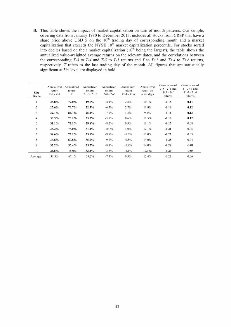
43

B. This table shows the impact of market capitalization on turn of month patterns. Our sample, covering data from January 1980 to December 2013, includes all stocks from CRSP that have a share price above USD 5 on the 10th trading day of corresponding month and a market capitalization that exceeds the NYSE 10th market capitalization percentile. For stocks sorted into deciles based on their market capitalization (10th being the largest), the table shows the annualized value-weighted average returns on the relevant dates, and the correlations between the corresponding T-8 to T-4 and T-3 to T-1 returns and T to T+3 and T+4 to T+8 returns, respectively. T refers to the last trading day of the month. All figures that are statistically significant at 5% level are displayed in bold.

Size Decile

Annualized return

T-3 - T-1

Annualized return

T

Annualized return

T+1 - T+3

Annualized return

T-8 - T-4

Annualized return

T+4 - T+8

Annualized return on

other days

Correlation of T-8 - T-4 and

T-3 - T-1 returns

Correlation of T - T+3 and T+4 - T+8

returns

1 25.8% 77.0% 19.6% -4.1% 2.8% 10.1% -0.18 0.11

2 27.6% 76.7% 22.5% -6.5% 2.7% 11.9% -0.16 0.12

3 32.1% 84.7% 25.1% -7.9% 1.3% 9.1% -0.16 0.13

4 33.5% 76.2% 25.3% -5.9% 0.6% 11.5% -0.18 0.12

5 31.1% 73.1% 29.8% -8.2% 0.3% 11.1% -0.17 0.08

6 35.2% 75.0% 31.1% -10.7% 1.0% 12.1% -0.21 0.05

7 34.6% 73.1% 33.9% -9.8% -1.0% 13.0% -0.22 0.03

8 34.6% 60.8% 35.9% -9.7% -0.8% 14.0% -0.28 0.04

9 32.2% 56.4% 35.2% -8.1% -1.8% 14.0% -0.28 -0.01

10 26.5% 18.0% 33.4% -3.5% -2.1% 17.1% -0.29 -0.08

Average 31.3% 67.1% 29.2% -7.4% 0.3% 12.4% -0.21 0.06

44

Table 8

Stock-level volatility and turn of the month patterns This table shows the effect of the stocks’ past 6-month return volatility on their turn of month patterns. To control for the fact that liquidity and volatility are correlated we condition our volatility estimates on liquidity. Our sample, covering data from 1980 to 2013, includes all stocks in CRSP listed in NYSE and Amex that have share price above USD 5 on the 10th trading day of corresponding month, and a market capitalization that exceeds the NYSE 10th market capitalization percentile. Amihud (2002) ILLIQ measure is calculated as a rolling one year average until the 10th trading day of corresponding month. Stocks fulfilling the requirements stated above are first divided into Amihud-illiquidity quartiles; quartile 1(4) denoting the most liquid (illiquid) stocks. Then every Amihud-illiquidity quartile is divided into volatility quartiles; quartile 1 (4) denoting the least (most) volatile stocks within the Amihud-illiquidity quartile. The reported results relate to the value-weighted returns of the Amihud-Volatility sorted portfolios. T refers to the last trading day of the month. All figures that are statistically significant at 5% level are displayed in bold.

Amihud Volatility

Annualized return

T-3 - T-1

Annualized return

T

Annualized return

T+1 - T+3

Annualized return

T-8 - T-4

Annualized return

T+4 - T+8

Annualized return on

other days

Correlation of T-8 - T-4 and

T-3 - T-1 returns

Correlation of T - T+3 and T+4 - T+8

returns

1 1 23.1% 15.0% 25.2% -1.4% 1.3% 18.1% -0.18 -0.12

1 2 33.9% 16.0% 30.8% -2.7% 0.0% 20.9% -0.24 -0.09

1 3 31.7% 24.7% 35.7% -6.5% -3.0% 14.8% -0.33 -0.02

1 4 30.5% 41.6% 41.2% -10.2% -8.4% 8.4% -0.40 -0.04

2 1 32.7% 47.1% 29.5% -3.2% 1.3% 20.4% -0.22 0.07

2 2 36.2% 61.8% 29.6% -7.5% -0.9% 19.1% -0.24 0.05

2 3 38.0% 67.5% 34.9% -11.0% -3.8% 16.5% -0.30 0.03

2 4 41.2% 73.7% 38.4% -17.8% -4.5% 13.6% -0.33 -0.01

3 1 31.5% 52.6% 30.2% -1.6% 2.0% 16.0% -0.23 0.07

3 2 36.7% 65.4% 30.4% -10.0% 3.0% 18.6% -0.26 0.06

3 3 43.5% 83.1% 33.1% -11.8% -3.1% 11.9% -0.25 0.04

3 4 37.7% 105.1% 35.1% -16.7% -7.4% 4.1% -0.29 0.06

4 1 25.2% 53.3% 27.4% 0.5% 7.8% 17.6% -0.17 0.14

4 2 36.6% 68.1% 28.9% -3.6% 5.4% 16.7% -0.24 0.09

4 3 32.2% 91.9% 30.4% -6.7% 1.9% 17.1% -0.27 0.06

4 4 42.8% 100.0% 30.0% -10.3% -0.2% 2.3% -0.21 0.06

Average 34.6% 60.4% 31.9% -7.5% -0.5% 14.7% -0.26 0.03

45

Table 9

Hedge fund excess market betas and redemption frequencies This table shows the hedge funds’ average excess market betas around the turn of the month and the hedge funds’ average excess market betas depending on the hedge funds’ redemption frequency (we have excluded all categories with less than 200 observations). T refers to the last trading day of the month. Hedge funds’ market betas are based on fund-specific regressions in which hedge fund’s (monthly) return is regressed on daily S&P 500 returns around the turn of the month and the return on the S&P500 index outside the turn of the month period. Excess market betas are calculated as a difference of the fund’s estimated beta for any given day and its beta for the outside the turn of the month period. Hedge fund data is from TASS and our sample period is from January 1994 to December 2013. T-statistics are shown below the coefficients. All figures that are statistically significant at 5% level are displayed in bold.

All funds Monthly Quarterly Semi-

Annually Annually T-5 -0.110 -0.123 -0.110 -0.039 -0.103

(-15.43) (-11.60) (-9.32) (-0.99) (-4.04) T-4 -0.089 -0.081 -0.118 -0.092 -0.113

(-12.04) (-7.54) (-10.43) (-1.78) (-3.65) T-3 -0.017 0.012 -0.058 -0.121 -0.112

(-2.54) (1.22) (-5.61) (-2.87) (-3.40) T-2 -0.088 -0.097 -0.083 -0.057 -0.010

(-13.26) (-9.96) (-8.27) (-1.23) (-0.39) T-1 -0.061 -0.041 -0.065 -0.097 -0.132

(-10.46) (-5.05) (-7.28) (-2.37) (-5.28) T -0.176 -0.173 -0.176 -0.121 -0.093 (-21.86) (-14.81) (-12.98) (-2.54) (-2.98)

T+1 0.142 0.134 0.171 0.112 0.163 (21.64) (14.56) (16.35) (2.85) (7.11)

T+2 0.250 0.227 0.260 0.355 0.348 (32.86) (20.42) (22.47) (6.58) (10.32)

T+3 0.164 0.141 0.188 0.241 0.238 (24.01) (13.78) (17.81) (5.26) (7.74)

T+4 0.106 0.079 0.145 0.125 0.121 (16.04) (8.73) (12.65) (2.96) (3.36)

T+5 0.038 0.017 0.071 0.091 0.146 (4.89) (1.54) (5.85) (2.10) (3.55) Average T-5 - T-3 -0.072 -0.064 -0.095 -0.084 -0.109 Average T-2 - T+5 0.047 0.036 0.064 0.081 0.097 Difference in averages 0.119 0.100 0.159 0.165 0.207

N 7,810 3,817 2,714 208 322

46

Table 10

Hedge fund excess market betas and styles

This table shows the hedge funds’ average excess market betas around the turn of the month in select hedge fund style categories. T refers to the last trading day of the month. Hedge funds’ average excess market betas are based on fund-specific regressions in which hedge fund’s (monthly) return is regressed on the daily S&P 500 returns around the turn of the month and the return on the S&P500 index outside the turn of the month period. Excess market betas for any given fund are calculated as a difference of its estimated beta for any given day and its beta outside the turn of the month period. Hedge fund data is from TASS and our sample period is from January 1994 to December 2013. T-statistics are shown below the coefficients. All figures that are statistically significant at 5% level are displayed in bold.

Global Macro

Managed Futures Other styles

T-5 -0.024 0.147 -0.134 (-0.62) (3.85) (-18.66)

T-4 -0.077 0.102 -0.104 (-1.63) (2.35) (-14.40)

T-3 0.106 0.424 -0.057 (2.36) (9.95) (-8.94)

T-2 -0.062 -0.052 -0.092 (-1.88) (-1.49) (-13.56)

T-1 0.091 -0.065 -0.068 (2.35) (-1.77) (-12.01) T -0.143 -0.092 -0.185 (-3.03) (-2.14) (-22.61)

T+1 0.052 0.191 0.142 (1.39) (4.74) (22.06)

T+2 0.066 0.213 0.261 (1.42) (5.44) (33.99)

T+3 0.100 0.089 0.173 (2.21) (2.14) (25.98)

T+4 0.044 -0.053 0.121 (1.09) (-1.40) (18.54)

T+5 -0.025 -0.046 0.047 (-0.67) (-0.93) (6.19) Average T-5 - T-3 0.001 0.224 -0.098 Average T-2 - T+5 0.016 0.023 0.050 Difference in averages 0.014 -0.201 0.148

N 314 538 6,958

47

Table 11

Funding conditions and turn of the month returns

This table shows the results from a regression in which the T-3 to T-1 stock market returns are regressed on the T-8 to T-4 market returns, a measure of cost of leverage, and its interaction with the T-8 to T-4 returns. T refers to the last trading day of the month. In the first two columns cost of leverage is measured with the TED spread (the difference between the 3-month Eurodollar and the Treasury rates). In the third and fourth column we modify the cost of leverage measure by multiplying the TED spread by the hedge fund industry’s assets under management and call this Hedge Funds’ Cost of Leverage. Hedge funds’ assets under management is the sum of all hedge funds’ assets under management based on HFR and TASS databases (calculated as in Jylhä and Suominen, 2011) divided by US stock market capitalization. The market index returns are those of the CRSP value-weighted index. T-statistics based on Newey-West standard errors are shown below the coefficients. All figures that are statistically significant at 5% level are displayed in bold.

y = Return T-3 - T-1

Return T-8 - T-4

-0.068

-0.075 (-1.17) (-1.36)

Cost of Leverage 0.004 (1.37)

Interaction of TED spread and the T-8 - T-4 return

-0.148 (-5.79)

Hedge funds’ Cost of Leverage

0.020 (0.69)

Interaction of hedge funds’ Cost of Leverage and the T-8 - T-4 return

-1.566

(-5.96)

Intercept 0.002 0.003

(1.15) (2.25)

R2 0.273 0.283

Sample 2/1991-12/2013

2/1991-12/2013

48

Table 12

Mutual fund alphas and exposures to month-end return reversals

This table shows active equity mutual funds’ annualized alphas conditional on fund-specific trailing two-year correlations between the funds’ T-8 to T-4 and T-3 to T-1 returns. More specifically, funds are divided into deciles every year (at the end of December) based on this correlation. Alphas are calculated using the subsequent year’s daily returns controlling for the three factors of Fama and French and Carhart’s Momentum factor. Panel A shows equally-weighted average of fund specific alphas and risk exposures and Panel B alphas and risk exposures based on equally-weighted mutual fund portfolio returns. Decile 10 contains the funds with the highest correlation in their T-8 to T-4 and T-3 to T-1 returns. The daily returns of active domestic equity mutual funds are from CRSP. The sample period is from January 1999 to December 2013. A: Equal-weighted average of fund specific alphas and risk exposures

Mutual fund deciles based on correlation of T-8 - T-4 and T-3 - T-1 returns

1 2 3 4 5 6 7 8 9 10 10-1

Alpha -1.13% -2.13% -1.98% -1.94% -1.85% -1.78% -1.47% -1.47% -0.97% 1.42% 2.55%

(-6.12) (-15.87) (-14.73) (-15.22) (-14.00) (-13.19) (-10.69) (-9.77) (-5.66) (4.85)

RM 0.94 0.98 0.99 0.99 0.99 0.99 0.98 0.99 0.97 0.88 -0.06

(211.41) (318.93) (297.23) (278.21) (262.35) (293.78) (271.14) (282.58) (236.31) (127.33)

SMB 0.14 0.13 0.16 0.18 0.20 0.21 0.26 0.26 0.29 0.29 0.15

(21.30) (20.10) (23.91) (26.24) (28.31) (29.53) (34.82) (34.83) (37.41) (36.63)

HML 0.03 0.01 0.00 -0.01 0.00 0.00 0.02 0.02 0.01 0.03 0.00

(3.93) (1.51) (-0.72) (-2.27) (-0.33) (0.50) (2.61) (2.46) (0.78) (3.48)

MOM 0.01 0.00 0.01 0.02 0.03 0.04 0.03 0.03 0.05 0.06 0.05

(1.83) (1.21) (1.37) (5.86) (6.89) (11.35) (8.39) (8.22) (10.84) (8.70)

B: Alpha and risk exposures of equal-weighted mutual fund portfolios

Mutual fund deciles based on correlation of T-8 - T-4 and T-3 - T-1 returns

1 2 3 4 5 6 7 8 9 10 10-1

Alpha -1.75% -2.56% -2.33% -2.14% -1.77% -1.42% -0.87% -0.49% 0.31% 2.76% 4.51%

(-1.47) (-3.18) (-3.45) (-3.57) (-3.53) (-2.79) (-1.63) (-0.72) (0.36) (1.89)

RM 0.98 1.01 1.01 1.00 1.00 1.00 0.98 0.99 0.97 0.87 -0.11

(83.97) (148.07) (175.00) (232.77) (309.33) (340.57) (277.79) (215.78) (176.20) (85.74)

SMB 0.21 0.17 0.18 0.19 0.21 0.22 0.26 0.26 0.27 0.24 0.03

(7.32) (11.97) (17.64) (22.05) (30.40) (33.66) (31.53) (23.60) (18.61) (8.75)

HML 0.09 -0.06 -0.04 -0.01 0.02 0.06 0.07 0.13 0.13 0.08 -0.01

(4.19) (-3.11) (-3.77) (-1.34) (2.51) (4.93) (6.06) (7.19) (6.23) (3.15)

MOM -0.11 -0.08 -0.05 -0.02 -0.01 0.03 0.05 0.08 0.12 0.16 0.27

(-10.24) (-9.19) (-6.89) (-2.88) (-0.87) (4.74) (8.18) (10.42) (14.21) (12.08)

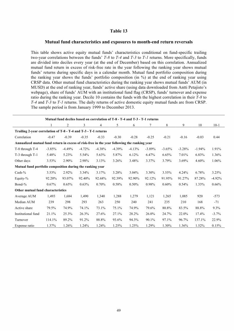
49

Table 13

Mutual fund characteristics and exposures to month-end return reversals

This table shows active equity mutual funds’ characteristics conditional on fund-specific trailing two-year correlations between the funds’ T-8 to T-4 and T-3 to T-1 returns. More specifically, funds are divided into deciles every year (at the end of December) based on this correlation. Annualized mutual fund return in excess of risk-free rate in the year following the ranking year shows mutual funds’ returns during specific days in a calendar month. Mutual fund portfolio composition during the ranking year shows the funds’ portfolio composition (in %) at the end of ranking year using CRSP data. Other mutual fund characteristics during the ranking year shows mutual funds’ AUM (in MUSD) at the end of ranking year, funds’ active share (using data downloaded from Antti Petajisto’s webpage), share of funds’ AUM with an institutional fund flag (CRSP), funds’ turnover and expense ratio during the ranking year. Decile 10 contains the funds with the highest correlation in their T-8 to T-4 and T-3 to T-1 returns. The daily returns of active domestic equity mutual funds are from CRSP. The sample period is from January 1999 to December 2013.

Mutual fund deciles based on correlation of T-8 - T-4 and T-3 - T-1 returns 1 2 3 4 5 6 7 8 9 10 10-1

Trailing 2-year correlation of T-8 - T-4 and T-3 - T-1 returns Correlation -0.47 -0.39 -0.35 -0.33 -0.30 -0.28 -0.25 -0.21 -0.16 -0.03 0.44

Annualized mutual fund return in excess of risk-free in the year following the ranking year T-8 through T-4 -3.85% -4.49% -4.72% -4.38% -4.39% -4.13% -3.89% -3.65% -3.28% -1.94% 1.91%

T-3 through T-1 5.48% 5.23% 5.54% 5.63% 5.87% 6.12% 6.47% 6.65% 7.01% 6.83% 1.36%

Other days 3.53% 2.90% 2.98% 3.13% 3.26% 3.48% 3.37% 3.79% 3.69% 4.60% 1.06%

Mutual fund portfolio composition during the ranking year Cash-% 3.53% 2.92% 3.34% 3.17% 3.28% 3.04% 3.30% 3.55% 4.24% 6.78% 3.25%

Equity-% 92.20% 93.07% 92.40% 92.68% 92.39% 92.90% 92.12% 91.95% 91.27% 87.28% -4.92%

Bond-% 0.67% 0.65% 0.63% 0.70% 0.58% 0.50% 0.98% 0.60% 0.54% 1.33% 0.66%

Other mutual fund characteristics Average AUM 1,493 1,684 1,490 1,340 1,288 1,279 1,121 1,265 1,085 920 -573

Median AUM 239 298 293 263 250 240 241 235 210 168 -71

Active share 79.5% 74.9% 74.1% 73.1% 75.1% 74.9% 79.6% 80.8% 83.5% 88.8% 9.3%

Institutional fund 21.1% 25.3% 26.3% 27.6% 27.1% 28.2% 26.0% 24.7% 22.0% 17.4% -3.7%

Turnover 114.1% 89.2% 91.2% 88.8% 93.6% 94.3% 90.1% 97.1% 96.7% 137.1% 22.9%

Expense ratio 1.37% 1.26% 1.24% 1.24% 1.25% 1.25% 1.29% 1.30% 1.36% 1.52% 0.15%

50

APPENDIX Table A1

Return patterns around the 15th (calendar) day of the month

Let S refers to the last trading day of the month that equals or precedes the 15th calendar day of the month. This table presents annualized returns around the day S in G-10 countries as well as in several other industrialized countries. In addition, the table presents the correlation of the returns from S-8 to S-4 and S-3 to S-1; as well as the correlation of the returns from S to S+3 and S+4 to S+8. Our sample starts in January 1980 or later as the relevant data becomes available, and settlement rule is T+3 or shorter. For the US we show also the full sample results. The sample runs until the end of 2013. All figures that are statistically significant at 5% level are displayed in bold.

Sample starts

Annualized return

S-3 - S-1

Annualized return

S

Annualized return

S+1 - S+3

Annualized return

S-8 - S-4

Annualized return

S+4 - S+8

Correlation of S-8 - S-4 and

S-3 - S-1 returns

Correlation of S - S+3 and S+4 - S+8

returns Country

United States (S&P 500) Jul-95 17.1% -9.0% 21.8% -2.3% -0.8% -0.26 -0.06

United States (CRSP VW) Jul-95 14.0% -11.7% 20.0% -3.5% 1.6% -0.26 -0.08

United States (S&P 500) Jan-80 18.7% 3.5% 11.4% 1.6% 7.0% -0.17 -0.04

United States (CRSP VW) Jan-80 16.6% 1.1% 7.9% 2.0% 7.1% -0.16 -0.01 Other industrialized countries

Australia (S&P/ASX200) Feb-99 -5.4% 7.5% 2.0% 4.9% 7.5% -0.04 -0.01

Austria (ATX) Feb-98 -6.7% -34.4% 2.7% 8.7% 9.5% -0.24 0.04

Belgium (BEL20) Jan-90 5.5% 8.6% 5.1% 4.4% -7.6% -0.11 0.09

Canada (S&P/TSX C) Jul-95 0.3% -9.8% 22.5% -2.3% 7.2% -0.17 -0.10

Denmark (OMXC20) Dec-89 9.2% 11.2% 6.1% 8.5% -6.6% -0.10 0.05

Finland (OMXH25) Jan-91 -5.1% -4.7% 23.2% 17.2% 7.8% -0.11 -0.05

France (CAC40) Oct-00 -1.3% -19.1% 7.9% -16.0% -9.6% -0.25 -0.05

Ireland (ISEQ OVER) Mar-01 -18.3% -24.1% 0.7% 0.0% -9.2% -0.17 0.01

Italy (FTSE MIB) Jan-98 9.1% -25.2% 12.7% -9.2% -5.1% -0.28 0.06

Japan (NIKKEI225) Jan-80 -11.1% 35.3% -4.3% 3.9% 6.5% -0.10 0.03

Luxembourg (LUXX) Jan-99 -1.2% -20.0% -4.3% -1.5% 1.6% -0.05 0.04

Netherlands (AEX) Jan-83 2.1% 16.4% 12.2% 12.7% 1.5% -0.17 0.10

New Zealand (NZX50) Jan-01 -3.1% -1.7% 4.4% 0.9% 10.0% -0.02 0.01

Norway (OBX) Jan-87 7.1% -0.3% -0.5% 5.6% 7.0% -0.12 -0.04

Portugal (PSI-20) Dec-98 -8.4% -31.5% -12.2% 12.0% -11.7% -0.16 0.03

Singapore (STI) Sep-99 -1.8% -17.3% -22.6% 7.9% 3.1% 0.05 0.18

Spain (IBEX35) Mar-97 1.3% -31.3% 24.7% 13.7% -9.3% -0.09 -0.04

Sweden (OMXS30) Jan-86 6.3% -4.2% 8.8% 17.7% 6.4% -0.16 0.00

Switzerland (SMI) Jul-88 3.2% 6.6% 2.2% 11.0% -1.7% -0.17 0.10

UK (FTSE100) Aug-96 -8.5% -16.7% 11.4% 9.5% -1.4% -0.21 -0.02

Countries with settlement period less than T+3

Germany (DAX) Jan-80 2.4% 13.6% 14.5% 11.4% -4.3% -0.12 0.04

Hong Kong (HSI) Jan-80 4.8% 38.2% 4.6% 20.9% 8.5% 0.00 0.10

Israel (TA-25) Jan-92 -9.2% 37.7% 13.1% 23.3% 5.9% -0.02 -0.15

South Korea (KOSPI) Jan-80 -0.6% -2.9% -2.6% 19.7% -7.4% -0.12 0.03

Average of all indexes excluding US -1.2% -3.3% 5.5% 7.7% 0.4% -0.12 0.02