DART-BIO: Modelling the interplay of food, feed and fuels in a global CGE model

by Alvaro Calzadilla, Ruth Delzeit and Gernot Klepper

No. 1896 | January 2014

Kiel Institute for the World Economy, Hindenburgufer 66, 24105 Kiel, Germany

Kiel Working Paper No. 1896 | January 2014

DART-BIO: Modelling the interplay of food, feed and fuels in a global CGE model

Alvaro Calzadilla, Ruth Delzeit and Gernot Klepper

Abstract: Land use and land use change are determined as much by economic and institutional drivers as they depend on bio-physical conditions. Future pathways of socio-economic and environmental systems can only be assessed with scenarios which describe possible future paths of development. For this numeric models are one important tool. To capture the complex interactions between the development of regionally differentiated economic drivers, computable general equilibrium (CGE) models can be used. We discuss in a transparent way the inclusion of land and the representation of the complex agricultural production activities into DART-BIO, a CGE model. Implementing a scenario of changes in the preferences for meat and dairy products which is currently taking place in Asia, we find that these preference changes have only minor impacts on global agricultural prices while affecting regional production and trade. Results strongly depend on key parameter settings and highlight the importance of interlinkages between biofuel and livestock production.

Keywords: CGE Model, land use, biofuels, simulation model

JEL classification: C61, Q16, Q42 Alvaro Calzadilla Kiel Institute for the World Economy The Environment and Natural Resources D-24105 Kiel E-mail: alvaro.calzadilla@ifw-kiel.de Gernot Klepper Kiel Institute for the World Economy The Environment and Natural Resources D-24105 Kiel E-mail: gernot.klepper@ifw-kiel.de

Ruth Delzeit Kiel Institute for the World Economy The Environment and Natural Resources D-24105 Kiel E-mail: ruth.delzeit@ifw-kiel.de

____________________________________

The responsibility for the contents of the working papers rests with the author, not the Institute. Since working papers are of a preliminary nature, it may be useful to contact the author of a particular working paper about results or caveats before referring to, or quoting, a paper. Any comments on working papers should be sent directly to the author. Coverphoto: uni_com on photocase.com

1

1. Introduction

Land use and land use change is determined as much by economic and institutional drivers as it

depends on the bio-physical conditions, i.e. its suitability and its productivity. The demand for

different uses of biomass is increasing and thus land use change and the expansion of farming

areas into natural habitats may threaten ecosystems and their services. The factors influencing

this process include climate and demographic change but also an increasing globalisation of

agricultural markets paired with an increasing divergence between regional supply and demand

of biomass. In addition, agricultural production and agricultural markets highly depend on

numerous political interventions, e.g. on the support of biofuels. Finally, in the medium to long-

run the process of global change may also alter lifestyles and consumption patterns as we know

them today. Such future pathways of socio-economic and environmental systems can only be

assessed with scenarios which describe possible future paths of development. For this numeric

models are one important tool. To capture complex interactions between the development of

regionally differentiated economic drivers, computable general equilibrium (CGE) models can

be used to analyse effects of this interplay of different factors influencing the agricultural

sectors. However, modelling land use change gives rise to a number of methodological

challenges: first, the representation of land as a heterogeneous input factor is not common in

the standard CGE-models. Treating it heterogeneously gives the possibility to correctly take into

account changing land uses, but requires information on suitability of crops and mechanism of

land allocation. Second, many models are so far not suited to adequately represent the

complex production and value change of agricultural goods, especially the multi-functionality of

many agricultural raw materials and the multi-product aspect of many farming activities. And

finally, the GTAP database which most CGE models use does not contain important feedstocks

used in the biofuel industries such as maize or certain plant oils.

Therefore, this paper aims to discuss in a transparent way the inclusion of land and the

representation of the complex agricultural production activities into a CGE model. In particular,

we present an approach with which both the special aspects of biofuels as well as the changes

in the consumption preferences for different agricultural products can be integrated into a CGE

model. The new DART-BIO model is an advancement of the Dynamic Applied Regional Trade

(DART) Model (Springer 2002). We pay special attention to by-products of biofuel production

since they turn out to be one of the most important determinants of the market effects of

2

biofuel policies and since they provide an important link between biofuels and livestock

production. The importance of the interlinkages between biofuel and livestock production is

highlighted by showing the results for a scenario of changes in the preferences for meat and

dairy products which is currently taking place in Asia.

The paper is structured as follows: First, we provide a literature overview on how land is

integrated in other CGE models and point out key aspects that need to be considered when

modelling land use and land use change. In section 3, we introduce a new version of the DART

model, named DART-BIO, which treats land as a heterogeneous production factor and which

includes a detailed representation of biofuels its feedstocks and by-products. To discuss the

performance of the model, in section 4 we present a scenario in which we change the

preferences for the consumption of meat and dairy products in selected regions in order to

illustrate key features and sensitive parameters of the modelling exercise.

2. Literature overview on approaches to model land use change in CGE models

The heterogeneity of land did not use to be explicitly modelled in most CGE models until they

were applied to simulate impacts of biofuel targets on land use. With the promotion of biofuels

in many countries and concerns about competition on land for primary factors to produce

biofuels, land was integrated into many models (see section 2.2). In this section, we first

provide an overview on data available to model land use, and discuss approaches of how land is

integrated into CGE models.

2.1 Land use data in the GTAP database

2.1.1 Data description

Land enters production of agricultural goods as an input factor and is usually represented by

land rents generated in Agro-Ecological Zones (AEZ). Original data on land use in GTAP7

database (GTAP-AEZ) is based on global land cover and land use data bases documented in

Monfreda et al. (2008) and Ramankutty and Foley (1999), Ramankutty et al. (2008) as well as

global forestry data by Sohngen and Tennity (2004). The GTAP7 land use data has been updated

to GTAP8 (Baldos & Hertel 2012).

3

Definition of AEZs in GTAP

For the Center for Sustainability and the Global Environment (SAGE), Ramankutty and Foley

(1999) collected data back to 1700 on historical inventory data on cropland areas and derived a

global dataset of potential natural vegetation types (Ramankutty and Foley 1998). The SAGE

database also includes data from National Geographic Maps 2002 and Foley et al. (2003) on the

world`s grazing land and build-up areas (for the early 90s). A first version of the GTAP-Agro-

Ecological Zones consisted of data by Lee et al. (2005) who used the dataset by Ramankutty and

Foley (1998) to derive spatial distributions of 19 crop types.

The second version of GTAP-AEZ is based on a new dataset: Since remote sensing data is limited

in their ability to resolve the details of agricultural land cover from space, SAGE has developed a

methodology, in which remote sensing data is “fused” with administrative-unit-level data on

land use (Monfreda et al. 2011). Focusing on agricultural crops and grazing land, a global

dataset for the period of about 2000 was developed by Ramakutty et al. (2008). They present a

detailed database of global land use practices describing the harvested areas and yields of 175

FAO crops circa the year 2000 at a 5 min by 5 min spatial resolution. This data is derived by

combining a gridded map of global cropland for the year 2000 and agricultural statistics from

national and FAO databases. The agricultural statistics are derived by correcting area and yield

data for individual years from 1990-2003, followed by a determination of values for average

years resulting in data for about the year 2000. For more detailed information see Ramankutty

et al. (2008).

The methodology for integrating this information on land cover and use into the GTAP-AEZ

framework is documented by Monfreda et al. (2011), Lee et al. (2011) and Avetisyan et al.

(2010). In a first step, they aggregate the 175 FAO crops into eight sectors. Secondly, the sector

land is disaggregated into 18 Agro-Ecological Zones according to six global Length of Growing

Period (LGP) classes times three climate zones (see Monfreda et al. 2011). In a second step, the

data on the eight GTAP crop sectors is allocated to the AEZ and the distribution of production is

determined by multiplying harvested area by yield, and then by price at the 175 crop level.

Summing over the 175 FAO crops results in values for the eight GTAP crop sectors. As for crops,

land rents for pasture and forest are included into the GTAP database.

Land rents for the livestock sector on pasture land are derived by a different approach. It is

assumed that the sector “ruminants” directly consumes land. Total grazing area is taken from

4

Ramankutty et al. (2008) and an estimate of the relative productivity of these different land

areas in all types of ruminant production across AEZs is estimated. More details are provided in

section Annex C.

In order to represent forest in the database, data on total hectares of forest area, timber land

rent (in USD per hectare per year), timber production, timber log prices, stumpage prices, net

present value for different timber types, annually harvested forest area is collected by Sohngen

et al. (2011). Parts of this data is adjusted to AEZs by first, overlaying productions of the

distribution of different ecosystem types from Haxeltine and Prentice (1996) with global forest

data from Ramankutty and Forley (1999) to estimate the proportion of forestland residing in

each ecosystem type in each country (Sohngen et al. 2011). In a second step, the resulting

proportion is combined with total forest land estimates from FAO (2005) to determine the area

of forestland in each ecosystem type in each country. Third, country level estimates of the area

of forest in each age class and timber type within a country is developed by applying age class

distributions from Sohngen et al. (1999) and Sohngen and Mendelson (2003, 2007). This

resulting land area per forest type from these steps is then distributed to the AEZs. According to

step one, the AEZs definition by Ramankutty and Foley (1999) and ecosystem type map from

Haxeltine and Prentice (1996) is combined to generate an estimate of the proportion of land in

each ecosystem type that resides in each AEZ in order to distribute the timber types in each

country to AEZs (Sohngen et al. 2011). However, “it is not feasible to general corresponding

estimates of all the economic parameters in the dataset by AEZ. These economic parameters

include prices, costs, parameters for yield functions, factors of carbon sequestration etc.”

(Sohngen et al. 2009, p. 67). They are only available on the country-level, but are used for

generating land rents, as explained in the following section.

2.1.2 Adjusting data to GTAP-AEZs

Values on returns to 1) crop production, 2) livestock production on pasture and 3) timber area

are used to allocate land rents from the land sector of the GTAP database into 18 separate land

sectors. Lee et al. (2011) explain how existing land rents in the GTAP database are shared out

accordingly whereas land rents are generated by the activity on a given parcel of land during a

calendar year. By dividing land rents from the homogeneous factor land into 18 land types the

suitability of each AEZ for production of crops, livestock and forestry is evaluated based on

observed practices from literature. Thus, within a single AEZ competition for land across

5

different uses is constrained to comprise activities, which have been detected to having taken

place in that AEZ. Details are explained in Annex C.

2.1.3 Limitations of land use data

The land use dataset only contains the amount of land by AEZ used in each crop, but does not

contain data on the variation in use of labour and capital by crop and AEZ. The GTAP database

therefore assumes that the distribution of value-added across land, labour and capital is the

same across all agricultural activities in a country. Value-added shares thus differ across

countries but are identical for all agricultural activities within a country.

The agricultural sector is the main source of income for developing countries. Using data on

land rents does, however, not allow considering subsistence agriculture, which is the common

system in those countries.

2.2 Land as an input factor

Kretschmer & Peterson (2010) provide an overview on different approaches to model land use

in CGE models. They explain that the simplest approach to include land into the modelling

exercise, as performed by Dixon et al. (2007) and Kretschmer et al. (2009) is to treat the input

factor land as a homogenous factor of production in the agricultural sector that is fixed in

supply. However, land is a heterogeneous good in reality, and therefore, different land types

and uses need to be taken into consideration. This has been done in recent literature:

Since this land endowment enters the production functions for crops, land use change is driven

by price changes. Generally, land use change can take place within the land types that are

represented by land rents in the database (Al-Raiffi et al. (2010) call it substitution effect) and

land used for crop production can be extended to other land types (expansion effect). Land

uses included in the database are cropland, pastureland and managed forest, and they are

ascribed to some economic values (see section 2.1.1). The possibility to convert land from one

of these land uses to another is determined by substitution possibilities: several studies using

CGE models for capturing land use change, apply the Constant Elasticity of Transformation

(CET) approach (see e.g. Banse et al. 2008, Hertel et al. 2010, Bouët et al. 2010, Al-Raiffi et al.

2010, Laborde 2011, Laborde and Valin (2012)). In this approach, an increase in demand of one

product, e.g. wheat, leads to an increase in price and land is taken from another good, e.g.

maize, depending on the relative prices. If the elasticity between wheat and maize is high, land

6

use change will not result in large prices increases in case of a demand increase. If

transformation possibilities are low, a higher demand (e.g. caused by biofuel quotas) will raise

prices for managed land. Drawbacks of this approach are discussed in Golub et al. (2011). They

explain that it allows significant differences in returns to land in the same AEZ to persist over

time and that in a given AEZ the fundamental constraint in the CET production possibility

frontier for land is expressed in effective hectare (productivity weighted hectares) and not

physical hectares.

Some studies allow for an expansion into land uses that are not managed, have therefore no

value and are consequently not represented in the database (cp. Banse et al. 2008). In this case,

higher prices for managed land affect unmangaged land uses (land expansion).

Different land uses are represented by a nesting structure, which can include different levels

and different elasticities of transformation between the different land uses with levels of

nesting. Banse et al. (2008) for example, incorporated a three level CET nesting structure with

differing land use transformability across types of land use while the values of the elasticities

are taken from the OECD’s PEM model (Abler, 2000; Salhofer, 2000). Laborde and Valin (2012)

also use a multi-level CET approach. They calibrate transformation elasticities to fit land supply

elasticities from the FAPRI elasticity database. Additionally, they assume perfect substitution

within each region for location of production across AEZs. In these modelling approaches, land

rents for the single nesting levels enter into agricultural production functions.

In the following section, the new land-use version of the DART Model, DART-BIO model is

introduced.

3. DART-BIO

3.1 Introduction

The Dynamic Applied Regional Trade (DART) model is a multi-sectoral, multi-regional recursive

dynamic Computable General Equilibrium (CGE) model of the world economy. The DART model,

developed in the late 1990’s at the Kiel Institute for the World Economy, has been applied to

analyse international climate policies (e.g. Springer 1998; Klepper and Peterson 2006a),

environmental policies (e.g. Weitzel et al. 2012), energy policies (e.g. Klepper and Peterson

2006b), and agricultural and biofuel policies (e.g. Kretschmer et al. 2009) among others.

7

The DART model is based on the up-to-date data from the Global Trade Analysis Project (GTAP)

covering multiple sector and regions. The economy in each region is modelled as a competitive

economy with flexible prices and market clearing conditions. The dynamic framework is

recursively-dynamic meaning that the evolution of the economies over time is described by a

sequence of single-period static equilibria connected through capital accumulation and changes

in labour supply. The economic structure of DART is fully specified for each region and covers

production, investment and final consumption by consumers and the government.

3.2 Aggregation of DART-BIO

As in all CGE models, the DART model consists on behavioural equations that describe the

economic behaviour of each agent in the model, identity equations that impose constraints in

the model to ensure market clearing, macro closure rules that determine the macroeconomic

equilibrium conditions of the model and a detail empirical database consistent with the model

equations.

The DART-BIO model is calibrated based on the current GTAP8.1 database (Narayanan et al.

2012), which represents the global economy in 2007 and covers 57 sectors and 134 regions.

Sectors and regions are aggregated/extended depending on the question at hand. The current

DART-BIO model has 23 regions, 38 sectors, 45 products and 21 factors of production.

As the focus of the model is to analyse the dynamic effects of bioenergy and land use policies,

the regional aggregation is carefully chosen to include the main biofuel producing and

consuming countries such as the United States of America (USA), Brazil (BRA), Germany (DEU)

and France (FRA) among others (Table 1). The regional detail also includes countries where

their main land use changes either due to biofuels production or where major changes in

population, income and consumption patterns are expected to emerge (e.g. Malaysia,

Indonesia and China).

8

Table 1: List of regions in DART-BIO

EU (7) Non-EU (16)

DEU Germany USA USA

GBR United Kingdom, Ireland CAN Canada

FRA France ANZ Australia, New Zealand

SCA Finland, Sweden, Denmark JPN Japan

BEN Belgium, Netherlands, Luxemburg RUS Russia

MED Spain, Portugal, Italy, Greece, Malta, Cyprus FSU Rest of Former Soviet Union and Europe

REU Rest of European Union BRA Brazil

PAO Paraguay, Argentina, Uruguay, Chile

LAM Rest of Latin America

CHN China

IND India

MAI Malaysia, Indonesia

SEA South East Asia

MEA Middle East, North Africa

AFR Sub-Saharan Africa

ROW Rest of the World

To adequately model biofuel production several key sectors need to be considered

independently. Some of these sectors are not explicitly included in the original GTAP database

and therefore need to be carved out from embedded sectors. Thus, 23 new sectors/products

have been added to the standard GTAP database to model in total 38 sectors and 45 products

(Table 2). The current DART-BIO model includes ethanol production from sugar cane/beet,

wheat, maize and other grains; and biodiesel production from palm oil, soybean oil, rapeseed

oil and other oilseed oils. DART-BIO explicitly accounts for the by-products generated during

the production process of biofuels. Dried distillers grains with solubles (DDGS) are by-products

of the production of ethanol from grains and oilseed meals/cakes are by-products of the

vegetable oil industry. Thus, unlike the standard GTAP database, we differentiate between

production activities and commodities, which allows to model joint production in the ethanol

and vegetable oil industry.

In addition, as biofuel consumption targets in the European Union are set according to the use

of renewable energy in the road transport sector, the DART-BIO model includes individual

sectors for motor gasoline and motor diesel.

9

Table 2: List of sectors (industries) and products (goods) in DART-BIO

Agricultural related products (29) Energy products (13)

PDR Paddy rice COL Coal

WHT Wheat CRU Oil

MZE Maize GAS Gas

GRON Other cereal grains MGAS Motor gasoline

PLM Oil Palm fruit MDIE Motor diesel

RSD Rapeseed OIL Petroleum and coal products

SOY Soybean ELY Electricity

OSDN Other oil seeds ETHW* Ethanol from wheat

C_B Sugar cane and sugar beet ETHM* Ethanol from maize

OLVS Outdoor livestock ETHG* Ethanol from other grains

ILVS Indoor livestock ETHS Ethanol from sugar cane

AGR Rest of agriculture BETH Bioethanol

FRS Forestry BDIE Biodiesel

PLMoil* Palm oil

PLMmeal* Palm meal

RSDoil* Rapeseed oil Non-energy products (3)

RSDmeal* Rapeseed meal CRPN Other chemical rubber plastic prods

SOYoil* Soybean oil ETS Paper, minerals and metals

SOYmeal* Soybean meal OTH Other goods and services

OSDNoil* Oil from other oil seeds

OSDNmeal* Meal from other oil seeds

VOLN Other vegetable oils

SGR Sugar

FOD Rest of food

PCM Processed animal products

FRI Forest related industry

DDGSw* DDGS from wheat

DDGSm* DDGS from maize

DDGSg* DDGS from other cereal grains

Note: New products are highlighted in blue. All goods are produced by an analogous industry, except were indicated.

* indicates jointly produced goods. Ethanol and DDGS are jointly produced by the ethanol industry (3 types of industries); and oilseeds oil and meal are jointly produced by the vegetable oil industry (4 types of industries).

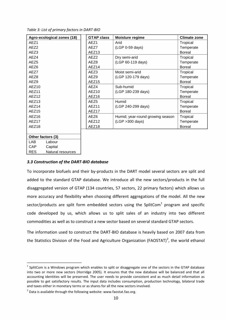
The DART-BIO model has been extended to incorporate the AEZ methodology (see Section 2.1).

Thus, we use 18 GTAP-AEZs, covering six different lengths of growing period spread over three

different climatic zones (Table 3). Previously, land in the DART model was a homogenous factor

of production use in the agricultural sector. By using the GTAP-AEZ framework, the current

version of the DART model accounts for land heterogeneity and within each AEZ and region,

land is allocated to different uses, i.e. cropland, pasture and forest.

10

Table 3: List of primary factors in DART-BIO

Agro-ecological zones (18) GTAP class Moisture regime Climate zone

AEZ1 AEZ1 Arid Tropical

AEZ2 AEZ7 (LGP 0-59 days) Temperate

AEZ3 AEZ13 Boreal

AEZ4 AEZ2 Dry semi-arid Tropical

AEZ5 AEZ8 (LGP 60-119 days) Temperate

AEZ6 AEZ14 Boreal

AEZ7 AEZ3 Moist semi-arid Tropical

AEZ8 AEZ9 (LGP 120-179 days) Temperate

AEZ9 AEZ15 Boreal

AEZ10 AEZ4 Sub-humid Tropical

AEZ11 AEZ10 (LGP 180-239 days) Temperate

AEZ12 AEZ16 Boreal

AEZ13 AEZ5 Humid Tropical

AEZ14 AEZ11 (LGP 240-299 days) Temperate

AEZ15 AEZ17 Boreal

AEZ16 AEZ6 Humid; year-round growing season Tropical

AEZ17 AEZ12 (LGP >300 days) Temperate

AEZ18 AEZ18 Boreal

Other factors (3) LAB Labour CAP Capital RES Natural resources

3.3 Construction of the DART-BIO database

To incorporate biofuels and their by-products in the DART model several sectors are split and

added to the standard GTAP database. We introduce all the new sectors/products in the full

disaggregated version of GTAP (134 countries, 57 sectors, 22 primary factors) which allows us

more accuracy and flexibility when choosing different aggregations of the model. All the new

sector/products are split form embedded sectors using the SplitCom1 program and specific

code developed by us, which allows us to split sales of an industry into two different

commodities as well as to construct a new sector based on several standard GTAP sectors.

The information used to construct the DART-BIO database is heavily based on 2007 data from

the Statistics Division of the Food and Agriculture Organization (FAOSTAT)2, the world ethanol

1 SplitCom is a Windows program which enables to split or disaggregate one of the sectors in the GTAP database

into two or more new sectors (Horridge 2005). It ensures that the new database will be balanced and that all accounting identities will be preserved. The user needs to provide consistent and as much detail information as possible to get satisfactory results. The input data includes consumption, production technology, bilateral trade and taxes either in monetary terms or as shares for all the new sectors involved. 2 Data is available through the following website: www.faostat.fao.org.

11

and biofuel reports published by F.O.Licht3 (F.O.Licht 2008, 2010 and 2011) and the production

costs for ethanol and biofuels provided by the meó Consulting Team4. This data is

complemented by the United Nations Statistics Division (UNSD)5, the BACI database6 and the

CAPRI model7. Below we provide a detailed explanation on the data and assumptions used to

split each of the new sectors/products in DART-BIO.

3.3.1 Maize (MZE)

Maize is an important feedstock for ethanol production. Almost half of the world ethanol is

produced from maize in the USA. The United States Department of Agriculture (USDA)

estimates that around 40% of the US maize is used in the ethanol industry, rising concerns

about its effect on food supply and food prices.

Maize in the standard GTAP database is part of the “cereal grains nec8” (GRO) sector which also

includes (Barley, Millet, Oats, Rye, Sorghum and other cereals). For splitting maize from GRO

we use 2007 production, price and bilateral trade data from FAOSTAT. For each commodity in

the GRO sector, we use producer price information to convert production in tonnes into USD

(currency unit in GTAP database). While total production in USD of “cereal grains nec” in FAO

and GTAP match in most of the regions there are some differences in regions like China and

Russia. These differences are compensated by using the FAO shares of maize production in total

GRO production to split GRO into maize (MZE) and the rest of other cereal grains (GRON). The

production technology for maize (MZE) and the other cereal grains (GRON) sector in each

country are assumed to be similar as those in the original GTAP sector (GRO).

Similarly, we use bilateral trade data from FAO to compute trade shares of maize in total GRO

trade for each bilateral trade flow. We assume that MZE and GRON have similar transportation

costs, tariffs, and export taxes or subsidies as the original GTAP GRO sector. The split of sales

3 F.O.Licht is a commodity analyst that report statistical data of a wide range of commodities including ethanol and

biodiesel (www.agra-net.net/agra/world-ethanol-and-biofuels-report). 4 meó Consulting Team is a company providing consulting services with a special focus on renewables sustainability

and climate change (www.meo-consulting.com). 5 Data is available through the following website: www.data.un.org.

6 BACI is a database of the world trade at a high level of product disaggregation developed by the French research

center in international economics (CEPII) (www.cepii.fr/anglaisgraph/bdd/baci.htm). It reconciles data provided by the United Nations Statistical Division (COMTRADE database). 7 The common agricultural policy regionalised impact analysis (CAPRI) model is a global agricultural sector model

with focus on the EU27, Norway, Turkey and Western Balkans. It has been designed to analyse the economic and environmental impact of agricultural policies and trade policies (www.capri-model.org). 8 Not elsewhere classified.

12

into the new two sectors to firms, households, the government and exports as well as changes

in stock are in proportion to the production shares and considering that total consumption of

each new sector must be equal to domestic consumption plus imports minus exports. The

resulting regional production of maize and other cereal grains is shown in Table A1, Annex A.

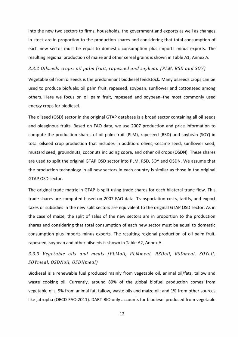
3.3.2 Oilseeds crops: oil palm fruit, rapeseed and soybean (PLM, RSD and SOY)

Vegetable oil from oilseeds is the predominant biodiesel feedstock. Many oilseeds crops can be

used to produce biofuels: oil palm fruit, rapeseed, soybean, sunflower and cottonseed among

others. Here we focus on oil palm fruit, rapeseed and soybean–the most commonly used

energy crops for biodiesel.

The oilseed (OSD) sector in the original GTAP database is a broad sector containing all oil seeds

and oleaginous fruits. Based on FAO data, we use 2007 production and price information to

compute the production shares of oil palm fruit (PLM), rapeseed (RSD) and soybean (SOY) in

total oilseed crop production that includes in addition: olives, sesame seed, sunflower seed,

mustard seed, groundnuts, coconuts including copra, and other oil crops (OSDN). These shares

are used to split the original GTAP OSD sector into PLM, RSD, SOY and OSDN. We assume that

the production technology in all new sectors in each country is similar as those in the original

GTAP OSD sector.

The original trade matrix in GTAP is split using trade shares for each bilateral trade flow. This

trade shares are computed based on 2007 FAO data. Transportation costs, tariffs, and export

taxes or subsidies in the new split sectors are equivalent to the original GTAP OSD sector. As in

the case of maize, the split of sales of the new sectors are in proportion to the production

shares and considering that total consumption of each new sector must be equal to domestic

consumption plus imports minus exports. The resulting regional production of oil palm fruit,

rapeseed, soybean and other oilseeds is shown in Table A2, Annex A.

3.3.3 Vegetable oils and meals (PLMoil, PLMmeal, RSDoil, RSDmeal, SOYoil,

SOYmeal, OSDNoil, OSDNmeal)

Biodiesel is a renewable fuel produced mainly from vegetable oil, animal oil/fats, tallow and

waste cooking oil. Currently, around 89% of the global biofuel production comes from

vegetable oils, 9% from animal fat, tallow, waste oils and maize oil; and 1% from other sources

like jatropha (OECD-FAO 2011). DART-BIO only accounts for biodiesel produced from vegetable

13

oil, covering in this way 90% of the global biodiesel production. We do not model second

generation9 biofuels because these technologies are currently under development and will

most probably have a small production share in 2020. However, DART-BIO has a very detailed

vegetable oil industry that allows to model with great detail oils and meals/cakes produced

from palm, rapeseed, soybean and other oilseeds.

The “vegetable oils and fats” (VOL) sector in the original GTAP database includes crude and

refined oils (from soybean, rape, coconut palm, palm kernel, maize, olive, sunflower-seed and

cotton-seed among others), animal or vegetable waxes, fats and oils; and their fractions

resulting from the extraction of vegetable oils and fats (cotton linters, oil-cake, flours, meals

and other solid residues). We use this sector to split the oils and part of the meals from palm,

rapeseed, soybean and other oilseeds. As noted by Al Riffai et al. (2010) and examining

carefully the GTAP database, most of the meals in GTAP are recorded under the “food products

nec” (OFD). Therefore, we use in addition the OFD sector to split the meals from palm,

rapeseed, soybean and other oilseeds.

Splitting vegetables oils and meals from different sectors requires a special attention on the

shares of oils and meals for the different oilseed sectors. Table 4 shows the global average

extraction shares for each oilseed industry in DART-BIO. The shares were computed based on

production in monetary terms, using quantity information at a country level from FAO and price

information from USDA (2012) and IEA (2009).

Table 4: Global average extraction shares in the oilseed industry in per cent

Oilseeds Oil Meal

Oil palm fruit 98 2

Rapeseed 74 26

Soybean 41 59

Other oilseeds 81 19

Source: DART-BIO, based on FAO data, USDA (2012) and IEA (2009).

Note: Shares computed based on monetary terms.

9 The OECD-IEA (2010) provides a clear definition of first and second generation biofuels. Typical first generation

biofuels are sugarcane ethanol, starch-based or ‘corn’ ethanol, biodiesel and pure plant oil. The feedstock for producing first generation biofuels either consists of sugar, starch and oil bearing crops or animal fats that in most cases can also be used as food and feed or consists of food residues.

Second generation biofuels are those biofuels produced from cellulose, hemicellulose or lignin. Examples of second generation biofuels are cellulosic ethanol and Fischer-Tropsch fuels.

14

To facilitate the procedure a new VOL sector was created containing the oils and the meals

from palm, rapeseed, soybean and other oilseeds. This new VOL sector was then split into palm

oil (PLMoil), palm meal (PLMmeal), rapeseed oil (RSDoil), rapeseed meal (RSDmeal), soy oil

(SOYoil), soy meal (SOYmeal), oil from other oilseeds (OSDNoil10), meal from other oilseeds

(OSDNmeal) and the remaining of the vegetable oil sector (VOLN). The cost structure of each

oilseed industry is assumed to be similar to the original GTAP VOL sector. However, we

introduced a joint production approach that allows each oilseed industry to produce two

goods: the oil and the meal.

Sales from the oil products go to industry as intermediates, to household and government

consumption, to international markets and to changes in stock. The sales from the oil products

are split according to the production shares and considering that total consumption of each

new sector must be equal to domestic consumption plus imports minus exports. Instead, as

meals are mainly used as animal feed, sales from the meal products go exclusively to the indoor

and outdoor livestock sectors and part of them are traded in international markets.

For both oils and meals, we use bilateral trade data from FAO and price information from IEA

(2009) and USDA (2012) to compute trade shares of oils and meals in the total trade volume of

the new VOL sector. This is done for each bilateral trade flow. We assume that the oil and meal

products have similar transportation costs, tariffs, and export taxes or subsidies as the original

GTAP VOL and OFD sectors. The resulting regional production of oils and meals from palm,

rapeseed, soybean and other oilseeds as well as other vegetable oils is shown in Table A3,

Annex A.

3.3.4 Motor gasoline and motor diesel (MGAS, MDIE)

Ethanol and biodiesel are mainly used as road-transport fuels. Ethanol can be blended with

gasoline or used directly in slightly modified spark-ignition engines. Biodiesel can be blended

with traditional diesel fuel or used directly in compression-ignition engines. The letters “E” and

“B” are used to designate the ethanol and biodiesel content in the blend. Thus, E20 designates

a mixture of 20% ethanol and 80% gasoline; as it is the case of blending mandates in Brazil.

To assess the substitution between ethanol and biodiesel with conventional fossil fuel

consumption, we decided to explicitly model motor gasoline and motor diesel. The “petroleum,

10

OSDNoil accounts mainly for the oil produced from sunflower seed. Accordingly, OSDNmeal accounts for the sunflower seed cake.

15

coal products” (P_C) sector in the original GTAP database includes coke oven products, refined

petroleum products and processing of nuclear fuel. For splitting motor gasoline and motor

diesel from P_C we use production data from the United Nations Statistics Division, and price

and trade data from COMTRADE.

The GTAP P_C sector corresponds to the division 33 of the Central Product Classification (CPC)

version 1.1 from the United Nations Statistics Division. We combine this data with price

information from COMTRADE to compute the production shares of motor gasoline (MGAS) and

motor diesel (MDIE) in total petroleum and coal products which also includes: aviation gasoline,

bitumen asphalt, brown coal coke, coke-oven gas, coke-oven coke, gas coke, jet fuel, kerosene,

liquefied petroleum gas, lubricants, naphtha, petroleum coke, petroleum waxes, residual fuel

oil and white spirit/industrial spirit (OIL). We use these shares to split the original GTAP P_C

sector into MGAS, MDIE and OIL, assuming that the production technology in all new sectors

are similar to the original P_C sector in GTAP.

Similarly, we use bilateral trade and price data from COMTRADE to compute trade shares of

motor gasoline and motor diesel in total P_C trade for each bilateral trade flow. We assume

that MGAS, MDIE and OIL have similar transportation costs and taxes/subsides as the original

GTAP P_C sector, except for the ad valorem tax rates, which are computed using information

from the IEA (2012).

The energy data from the United Nations Statistics Division allows us to distinguish between

household and industry consumption of MGAS, MDIE and OIL. Government consumption and

changes in stock are split using the production shares and considering total consumption of

each new sector must be equal to domestic consumption plus imports minus exports. The

resulting regional production of motor gasoline, motor diesel and other oil and coal products is

shown in Table A4, Annex A.

3.3.5 Biofuels: Ethanol and Biodiesel

In the last decade, global biofuel production and consumption has rapidly grown as countries

shift to a new energy mix to reduce dependence on fossil fuel and lower greenhouse gas (GHG)

emissions. However, biofuel development have also rise concerns about potential negative

impacts on food security, biodiversity, water resources and land use through an intensive

production of biofuel feedstocks.

16

To capture these interactions under a general equilibrium perspective, the DART-BIO model

includes 4 different types of ethanol and 4 different types of biodiesel: Ethanol produced from

sugar cane/beet, maize, wheat, and other cereals, and biodiesel produced from palm,

rapeseed, soybean and other oilseeds. Figure 1 shows the global ethanol and biodiesel

production by feedstock. This Figure summarizes the structure of the biofuel market in DART-

BIO and is the final output of the construction of the biofuel database (explained in detail

below).

Figure 1: Global ethanol and biodiesel production by feedstock (2007)

Source: DART-BIO.

Note: Palm oil (PLMoil); Rapeseed oil (RSDoil); Soy oil (SOYoil); Other (OSDNoil).

To assess correctly the land-use effects of bioenergy development, it is necessary to account for

by-products generated during the production process of biofuels. In the grain-based production

of ethanol, DDGS is a by-product which is used as animal feed. In the oilseed-based production

of biodiesel, oilseed meal or cake remains as a by-product that can be used as animal feed.

Glycerine, is another by-product in biodiesel production which can be used for industrial

purposes. The DART-BIO model includes 3 different types of DDGS and 4 different types of

meals/cakes as by-products of biofuel production: DDGS from maize, wheat and other grains,

and meals/cakes from palm, rapeseed, soybean and other oilseeds.

Bioethanol (ETHs, ETHm, ETHw, ETHg, ETH)

Biofuel sectors are not explicitly included in the current GTAP database. Therefore, we

disaggregated biofuel production, consumption and trade directly from the social accounting

matrices (SAM), ensuring that the national and global SAMs are kept balanced. As a first step,

we constructed an ethanol balance sheet that records production, exports, imports and

consumption in physical terms for each of the countries in the GTAP database. This balance

Maize57%

Sugar34%

Wheat8%

Other grains

1%

Ethanol(30,131 million USD)

RSDoil53%

SOYoil36%

PLMoil9%

OSDNoil2%

Biodiesel(7,479 million USD)

17

sheet is largely based on the world ethanol and biofuel reports published by F.O.Licht and

complemented by the database of the CAPRI model. Using market price information for

ethanol, this balance sheet is expressed in monetary terms. We use a global price of ethanol of

52 US dollar (USD) cents per litre (l) and specific prices for Brazil (37 USD cent/l), the US (56 USD

cent/l) and Germany (64 USD cent/l). These prices are based on statistics from the Brazilian

Sugarcane Industry Association (UNICA 2013), IEA (2008) and personal communication with the

meó Consulting Team. A corresponding subsidy has been calibrated to ensure a market

penetration of ethanol such as the share of ethanol in total motor gasoline consumption

matches the statistical data for the calibration year 2007.

The exports and imports in the ethanol balance sheet are consistent with a detailed trade

matrix constructed based on the reports published by F.O.Licht and complemented by the data

base of the CAPRI model. By constructing the trade matrix we paid special attention on

avoiding double accounting, thus we exclude re-exports of ethanol and include only

transactions from producer countries to the final consumer countries. Indeed, even if official

statistics show that US imports ethanol from Caribbean countries, this is just the re-export of

Brazilian ethanol through these countries due to tariff and regulation reasons.11

Figure 2 shows that the US and Brazil are the biggest producers and exporters of ethanol,

covering together around 75% of the production and 70% of the exports. Ethanol production on

other countries are marginal compared to the US and Brazil. Maize-based ethanol production in

China accounts for 7% and sugarcane-based ethanol production in India for 4%. Besides the US

and Brazil, ethanol exporting countries are France, Great Britain and Mediterranean countries,

the share of those countries in the global export market ranges between 5 to 7%.

11

Several Caribbean countries benefit from special duty free access to the US market, thus a joint ethanol production and refining program with Brazilian sugarcane producer gives them access to the US market at competitive prices (OECD-IEA 2006). In addition, the sugarcane-based ethanol qualifies as an “advanced” biofuel in the US Renewable Fuel Standard, while the maize-based ethanol only qualifies as “renewable” biofuel. This means that more blending credits are given for each litre of sugarcane-based ethanol compared to maize-based ethanol. Thus, the Brazilian sugarcane-based ethanol is a cheaper option to fulfil the US advanced biofuel requirements.

18

Figure 2: Top 5 producers, exporters and importers of bioethanol (2007)

Source: DART-BIO.

Note: Germany (DEU); UK, Ireland (GBR); France (FRA); Finland, Sweden, Denmark (SCA); Belgium, Netherlands, Luxemburg (BEN); Spain, Portugal, Italy, Greece, Malta, Cyprus (MED); Rest of European Union (REU); USA (USA); Canada (CAN); Australia, New Zealand (ANZ); Japan (JPN); Russia (RUS); Rest of Former Soviet Union and Europe (FSU); Brazil (BRA); Paraguay, Argentina, Uruguay, Chile (PAO); Rest of Latin America (LAM); China (CHN); India (IND); Malaysia, Indonesia (MAI); South East Asia (SEA); Middle East, North Africa (MEA); Sub-Saharan Africa (AFR); Rest of the World (ROW).

Even if the US is the biggest producer and second largest exporter of ethanol, it is also the

major importer of ethanol. The reason is behind the US regulations that differentiate between

maize-based ethanol (produced in the US) and sugarcane-based ethanol (imported from Brazil).

The US Renewable Fuel Standard classifies the sugarcane-based ethanol as “advanced” biofuel

and the maize-based ethanol as “renewable” biofuel. As “advanced” biofuels receive more

blending credits than “renewable” biofuels, importing sugarcane-based ethanol from Brazil

makes easier and cheaper to fulfil the US advanced biofuel mandates. The region “other Latin-

American countries” has the second largest share of ethanol imports (15%), followed by Canada

(12%), Benelux (7%) and Japan (7%).

We use production cost estimates by the meó Consulting Team (Table 5). We differentiate

three types of technologies: i) ethanol from sugar cane/beet, which is used to describe sugar

cane/beet-based ethanol production in all countries except Brazil; ii) ethanol from sugarcane in

Brazil and; iii) ethanol from cereal grains, which is used to describe cereal grain-based ethanol

production in all countries. These production costs are applied to each single country, taking

into account the countries’ shares of ethanol production by feedstock (sugar cane/beet, maize,

wheat and other grains).

USA48%

BRA28%

CHN7%

IND4%

FRA2%

Others11%

Production (30,131)

BRA54%

USA15%

FRA7%

GBR6%

MED5%

Others13%

Exports (2,179)

USA22%

LAM15%

CAN12%BEN

7%

JPN7%

Others37%

Imports (2,179)

19

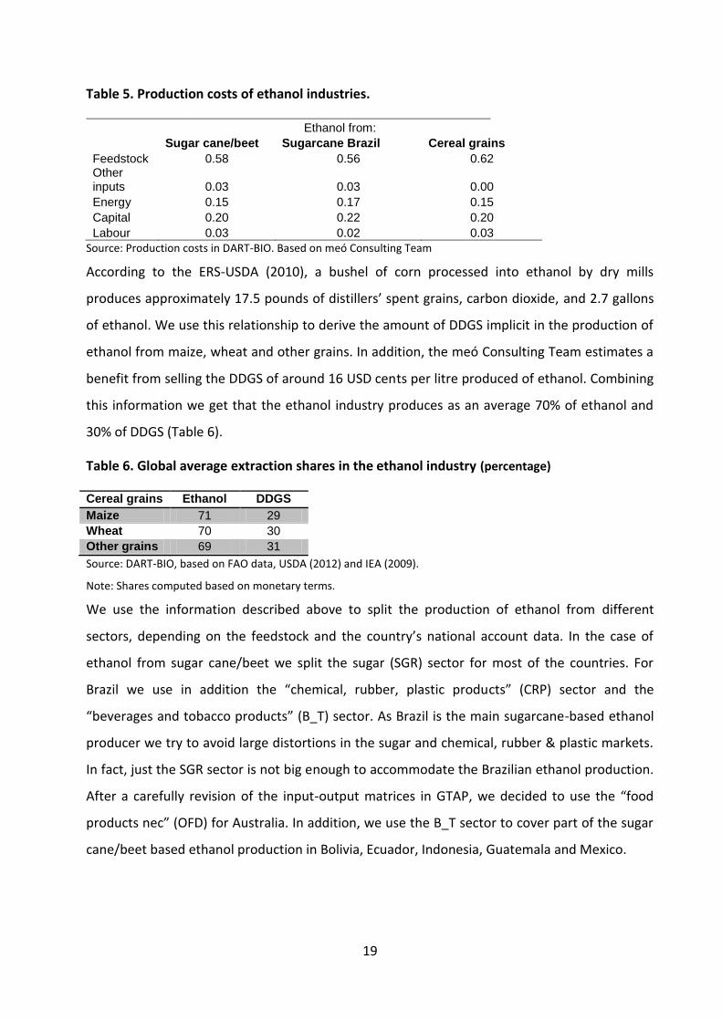
Table 5. Production costs of ethanol industries.

Ethanol from:

Sugar cane/beet Sugarcane Brazil Cereal grains

Feedstock 0.58 0.56 0.62 Other inputs 0.03 0.03 0.00

Energy 0.15 0.17 0.15

Capital 0.20 0.22 0.20

Labour 0.03 0.02 0.03

Source: Production costs in DART-BIO. Based on meó Consulting Team

According to the ERS-USDA (2010), a bushel of corn processed into ethanol by dry mills

produces approximately 17.5 pounds of distillers’ spent grains, carbon dioxide, and 2.7 gallons

of ethanol. We use this relationship to derive the amount of DDGS implicit in the production of

ethanol from maize, wheat and other grains. In addition, the meó Consulting Team estimates a

benefit from selling the DDGS of around 16 USD cents per litre produced of ethanol. Combining

this information we get that the ethanol industry produces as an average 70% of ethanol and

30% of DDGS (Table 6).

Table 6. Global average extraction shares in the ethanol industry (percentage)

Cereal grains Ethanol DDGS

Maize 71 29

Wheat 70 30

Other grains 69 31

Source: DART-BIO, based on FAO data, USDA (2012) and IEA (2009).

Note: Shares computed based on monetary terms.

We use the information described above to split the production of ethanol from different

sectors, depending on the feedstock and the country’s national account data. In the case of

ethanol from sugar cane/beet we split the sugar (SGR) sector for most of the countries. For

Brazil we use in addition the “chemical, rubber, plastic products” (CRP) sector and the

“beverages and tobacco products” (B_T) sector. As Brazil is the main sugarcane-based ethanol

producer we try to avoid large distortions in the sugar and chemical, rubber & plastic markets.

In fact, just the SGR sector is not big enough to accommodate the Brazilian ethanol production.

After a carefully revision of the input-output matrices in GTAP, we decided to use the “food

products nec” (OFD) for Australia. In addition, we use the B_T sector to cover part of the sugar

cane/beet based ethanol production in Bolivia, Ecuador, Indonesia, Guatemala and Mexico.

20

Trade of ethanol from sugar cane/beet is classified under the “beverages and tobacco

products” (B_T) sector in GTAP. We therefore use the B_T sector to split the bilateral trade

flows according to the constructed bilateral trade matrix.

In the case of ethanol from maize, wheat and other grains we split production and trade from

the OFD sector, which records the industrial processing of cereal grains. We use the ethanol

balance sheets to split the ethanol sectors by subtracting production, sales and trade from the

embedded sectors. While production subsidies have been calibrated to ensure the observed

market penetration of ethanol in total motor gasoline consumption; transportation costs,

tariffs, and export taxes/subsidies are assumed to be similar to those in the original embedded

GTAP sectors.

In DART-BIO, sales from all types of ethanol (from sugar cane/beet, maize, wheat and other

grains) are first collected by a blending sector (ETH) and then distributed to household

consumption and international markets (Figure 3). Instead, DDGS is only used as animal feed in

the domestic indoor and outdoor livestock sectors. Contrary to meals/cakes, we assume that

the by-product of the ethanol industry is not traded due to handling and storage limitations.

Figure 3: Scheme of ethanol production in DART-BIO

Biodiesel (BDIE)

Similar to the construction of the ethanol database, we first replicate the biodiesel market in a

balance sheet that records production, consumption, exports and imports for each country in

the GTAP database. This balance sheet is largely based on the world ethanol and biofuel reports

ETHW

WHT Ethanol industry Ethanol from wheat

Wheat from wheat

DDGSw Indoor and outdoor

Other intermediates DDGS from wheat livestock

and primary factors

ETHM

MZE Ethanol industry Ethanol from maize

Maize from maize

DDGSm BETH

Other intermediates DDGS from maize Bioethanol

and primary factors

ETHG

GRON Ethanol industry Ethanol from other grains

Other cereal grains from other grains

DDGSg Indoor and outdoor

Other intermediates DDGS from other grains livestock

and primary factors

C_B Ethanol industry ETHS

Sugar cane and beet from sugar cane Ethanol from sugar

Other intermediates

and primary factors

21

published by F.O.Licht and complemented by the database of the CAPRI model. As F.O.Licht

reports quantity data, we use market price information for biodiesel to express the balance

sheet in monetary terms. We use a global price of biodiesel of 80 USD cent/l, which is the

average of the 2007 market price in Brazil (108 USD cent/l), the USA (73 USD cent/l) and

Germany (86 USD cent/l). Price information is taken from the USDA/FAS (2010) and the meó

Consulting Team (personal communication). A corresponding subsidy has been calibrated to

ensure a market penetration of biodiesel such as the share of biodiesel in total motor diesel

consumption matches the statistical data for the calibration year 2007.

Contrary to other studies, we assume that biodiesel is produced using vegetable oils and not

directly from the oilseed crops (Figure 4). In DART-BIO, a vegetable oil industry produces two

goods: oils and meals/cakes. Part of the vegetable oils goes to the biodiesel industry and it is

combined with other intermediates and primary factors to produces biodiesel. The production

costs of the biodiesel industry are based on cost estimates made by the meó Consulting Team

(Table 6). We apply the same cost structure to all countries, differentiating only on the

appropriated feedstock for each country based on Ecofys-Agra CEAS-Chalmers University-IIASA-

Winrock (2011)

Figure 4: Scheme of biodiesel production in DART-BIO

Based on the reports published by F.O.Licht and complemented by the database of the CAPRI

model, we constructed a detailed trade matrix for biodiesel which is consistent with the

biodiesel balance sheet. As in the case of ethanol trade, we exclude re-exports of biodiesel.

PLMoil

PLM Vegetable oil industry Palm fruit and kernel oil

Palm fruit and kernel from palm fruit and kernel

PLMmeal

Other intermediates from palm fruit and kernel Other

and primary factors industries

RSDoil

RSD Vegetable oil industry Rapeseed oil

Rapeseed from rapeseed

RSDmeal

Other intermediates from rapeseed BDIE

and primary factors Biodiesel

SOYoil

SOY Vegetable oil industry Soybean oil

Soybean from soybean

SOYmeal

Other intermediates from soybean Other

and primary factors industries

OSDN

OSDN Vegetable oil industry Oil from other oilseeds

Other oilseeds from other oilseeds

OSDNmeal

Other intermediates from other oilseeds

and primary factors

Other intermediates

and primary factors

22

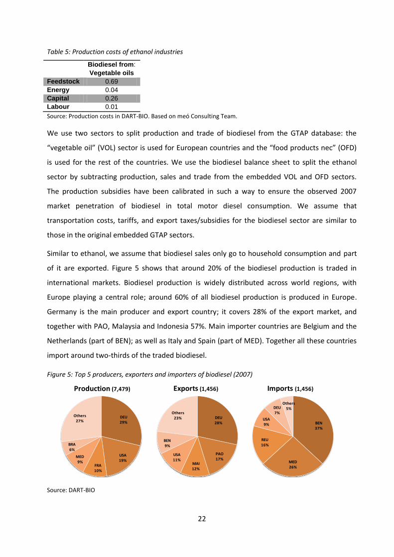
Table 5: Production costs of ethanol industries

Biodiesel from:

Vegetable oils

Feedstock 0.69

Energy 0.04

Capital 0.26

Labour 0.01

Source: Production costs in DART-BIO. Based on meó Consulting Team.

We use two sectors to split production and trade of biodiesel from the GTAP database: the

“vegetable oil” (VOL) sector is used for European countries and the “food products nec” (OFD)

is used for the rest of the countries. We use the biodiesel balance sheet to split the ethanol

sector by subtracting production, sales and trade from the embedded VOL and OFD sectors.

The production subsidies have been calibrated in such a way to ensure the observed 2007

market penetration of biodiesel in total motor diesel consumption. We assume that

transportation costs, tariffs, and export taxes/subsidies for the biodiesel sector are similar to

those in the original embedded GTAP sectors.

Similar to ethanol, we assume that biodiesel sales only go to household consumption and part

of it are exported. Figure 5 shows that around 20% of the biodiesel production is traded in

international markets. Biodiesel production is widely distributed across world regions, with

Europe playing a central role; around 60% of all biodiesel production is produced in Europe.

Germany is the main producer and export country; it covers 28% of the export market, and

together with PAO, Malaysia and Indonesia 57%. Main importer countries are Belgium and the

Netherlands (part of BEN); as well as Italy and Spain (part of MED). Together all these countries

import around two-thirds of the traded biodiesel.

Figure 5: Top 5 producers, exporters and importers of biodiesel (2007)

Source: DART-BIO

DEU29%

USA19%

FRA10%

MED9%

BRA6%

Others27%

Production (7,479)

DEU28%

PAO17%

MAI12%

USA11%

BEN9%

Others23%

Exports (1,456)

BEN37%

MED26%

REU16%

USA9%

DEU7%

Others5%

Imports (1,456)

23

Note: Germany (DEU); UK, Ireland (GBR); France (FRA); Finland, Sweden, Denmark (SCA); Belgium, Netherlands, Luxemburg (BEN); Spain, Portugal, Italy, Greece, Malta, Cyprus (MED); Rest of European Union (REU); USA (USA); Canada (CAN); Australia, New Zealand (ANZ); Japan (JPN); Russia (RUS); Rest of Former Soviet Union and Europe (FSU); Brazil (BRA); Paraguay, Argentina, Uruguay, Chile (PAO); Rest of Latin America (LAM); China (CHN); India (IND); Malaysia, Indonesia (MAI); South East Asia (SEA); Middle East, North Africa (MEA); Sub-Saharan Africa (AFR); Rest of the World (ROW).

3.4 The theoretical structure of DART-BIO model

The DART model is based on microeconomic theory. In each region the economy is modelled as

a competitive economy with flexible prices and market clearing conditions. Agents represented

in the model are consumers, who maximise utility, producers, who maximise profits, and

regional governments. All industry sectors operate at constant returns to scale. The goods are

produced by a combination of intermediate inputs (energy and non-energy inputs) and primary

factors (labour, capital and land in the agricultural sectors). The produced goods are directly

demanded by regional households, governments, the investment sector, other industries, and

the export sector. A representative household receives all income generated by providing

primary factors to the production process. Disposable income is used for maximising utility by

purchasing goods. The consumer saves a fixed share of income in each time period which is

invested in production. The government provides a public good financed by tax revenues.

Regions are connected via bilateral trade flows, where domestic and foreign goods are

imperfect substitutes and distinguished by country of origin (Armington assumptions). Factor

markets are perfectly competitive and full employment of all factors is assumed. Labour and

capital are assumed to be homogeneous goods, mobile across industries within regions but

internationally immobile. The primary factor land is only used in agriculture and exogenously

given. Below we provide a detailed explanation on the additions and changes to the standard

structure of the DART model described by Klepper et al. (2003).

3.4.1 Production

Producers are characterised by profit-maximization behaviour for a given output, at constant

returns to scale. Figure 6 shows the production structure for the agricultural and biofuel

sectors. It is based on a multi-level nested constant elasticity of substitution (CES) which

describes the technological possibilities in domestic production. On the top level of the

production function, there is a linear Leontief function (σ=0) of intermediate inputs and a value-

added–energy composite. The intermediate goods i in sector j correspond to a so-called

Armington aggregate of non-energy input from domestic production and imported varieties.

24

The value-added–energy composite is a CES function (σ=0.25) of land defined by AEZs and an

energy–capital–labour composite. The energy–capital–labour composite is a CES function

(σ=0.5) between energy and a capital–labour composite (aggregated by a Cobb-Douglas

function, σ=1).

For agricultural crops, the intermediate inputs composite is obtained by combining all non-

energy inputs using a Leontief technology. In the case of biodiesel (BDIE), the different

vegetables oils used for biodiesel production are aggregated using a CES function which allows

higher possibilities of substitution between them. A CES function is also used in the case of the

ethanol blending sector (ETH) to aggregate the different types of ethanol.

Figure 6: Production structure: Biofuels and agricultural goods

Some products in DART-BIO are jointly produced by the same industry. Ethanol and DDGS are

jointly produced by the ethanol from grains industry and oilseeds oil and meal are jointly

produced by the vegetable oil industry. The production structure of these industries is

modelled differently (Figure 7) and includes the ethanol from maize, wheat and other cereals,

as well as the palm oil, rapeseed oil, soy oil and oil form other oil seeds.

Ethanol (oil) and DDGS (meals) are produced at fixed proportion depending on the specific

industry production process. This joint production is captured by a constant elasticity of

transformation (CET) function () (Figure 7). At the next stage, the domestic output of both

Capital Labour

Energy VA

CES s .5

KLELand or

AEZi

KLLE

Intermediate

inputs (other)

Pa1 ... PaN

Output Py

Cobb-Douglas

Leontief

Exported good Px Domestic good Pd

CES s .25

CET 2

CES s 1 (Biofuels)

Leontief (Agri. goods)

25

goods is allocated between exports and domestic sales on the assumption that suppliers

maximize sales revenue for any given aggregate output level, subject to imperfect

transformability between exports and domestic sales, expressed by a CET (2) function.

Figure 7: Production structure: Ethanol from grains and vegetable oils

As DDGS and meal/cake are used as animal feed, the production process of the livestock

sectors introduces a CES function with a high degree of substitution possibilities (σ=2) to

aggregate the different feedstock crops and the by-products generated during the production

process of biofuels. Figure 8 shows in detail the production structure of the outdoor and indoor

livestock sectors in DART-BIO.

KLE

composite

Intermediate

inputs composite

Ethanol from grains /

Vegetable oils

Leontief

Ethanol /

Oils

DDGS /

Meals

CET

CET 2CET 2

Exported

good

Domestic

good

Exported

good

Domestic

good

26

Figure 8: Production structure: Livestock

3.4.2 Consumption

Consumers maximise their utility functions subject to their budget constraints. They purchase

different goods depending on their relative prices, to obtain the consumption (utility) against

the lowest expenditure. A share of income is saved (and invested in production sectors). These

shares differ across regions, and are adjusted to the age structure of the populations. Produced

goods are directly demanded by the regional households and government, the investment

sector, other industries, and the export sector.

A CES utility function with unitary income elasticities was used in previous versions of DART.

Here we use a non-unitary income elasticities based on the Linear Expenditure System (LES)

approach (Stone, 1954). The representative consumer is split into two categories: a

‘subsistence consumer’ and a ‘surplus consumer’. The subsistence consumer category

represents the consumer’s basic demand. It is specified as a Leontief function, that is, no

substitution possibilities for different consumption commodities, with an exogenously given

size. The surplus consumer category reflects how additional income is spent, and has positive

substitution elasticities for the different consumption commodities. Though the surplus

(sometimes called ‘supernumerary’) part of consumption has unitary income elasticities, total

consumption does not. This is so, because for every commodity the division in ‘subsistence’ and

Capital Labour

Energy VA

CES s .5

KLELand or

AEZi

KLLE

Intermediate

inputs composite

Output Py

Cobb-Douglas

Leontief

Exported good Px Domestic good Pd

CES s .25

CET 2

Feedstock crops,

DDGS,

Meals

Animal feed

composite

Other goods

Pa1 ... PaN

Leontief

Leontief

CES s 2

27

‘surplus’ is different. For basic commodities, the major part of consumption is attributed to the

subsistence consumer, while for luxury commodities a relatively large part is attributed to the

surplus consumer. Intuitively, one can think of the introduction of the subsistence consumer as

changing the origin for the utility function of private households.

The expenditure function of the representative household is assumed to be a Cobb-Douglas

composite of an energy aggregate and a non-energy bundle. Within the non-energy

consumption composite, substitution possibilities are described by a Cobb-Douglas function of

Armington goods. Within the energy aggregate we introduce a CES function (σ=2-3) to

aggregate motor diesel, motor gasoline, ethanol and biodiesel in all regions but Brazil. The car

fleet in Brazil consists of a high share of flexible fuel cars. We therefore presume an elasticity of

substitution of 10 in Brazil. Figure 9 shows the structure of consumer behaviour.

Figure 9: Final consumption in DART-BIO

3.5 Integration of land into the DART model

In the DART-BIO model we use land rents according to AEZ based on the GTAP-AEZ database

(see section 3). In many CGE models, the constant elasticity of transformation (CET) approach is

applied which allows land to be transformed to different uses whereas the ease of

transformation is characterised by the elasticity of transformation. Different land uses are

represented by a nesting structure, which can include a) different levels and b) different

elasticities of transformation between the different land uses with levels of nesting. We

decided for a three level nesting, displayed in Figure 10 using elasticities (see Annex B).

Pac1 ... PacN

Other Armington

intermediate inputsEnergy composite

Final consumption

Cobb-Douglas

Cobb-Douglas

Motor gasoline,

Motor diesel,

Ethanol,

Biodiesel

Energy-Biofuels

Composite

Other energy

goods

Cobb-Douglas

CES s (2 - 3)

28

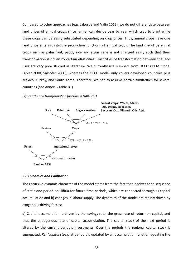
Compared to other approaches (e.g. Laborde and Valin 2012), we do not differentiate between

land prices of annual crops, since farmer can decide year by year which crop to plant while

these crops can be easily substituted depending on crop prices. Thus, annual crops have one

land price entering into the production functions of annual crops. The land use of perennial

crops such as palm fruit, paddy rice and sugar cane is not changed easily such that their

transformation is driven by certain elasticities. Elasticities of transformation between the land

uses are very poor studied in literature. We currently use numbers from OECD’s PEM model

(Abler 2000, Salhofer 2000), whereas the OECD model only covers developed countries plus

Mexico, Turkey, and South Korea. Therefore, we had to assume certain similarities for several

countries (see Annex B Table B1).

Figure 10: Land transformation function in DART-BIO

3.6 Dynamics and Calibration

The recursive-dynamic character of the model stems from the fact that it solves for a sequence

of static one-period equilibria for future time periods, which are connected through a) capital

accumulation and b) changes in labour supply. The dynamics of the model are mainly driven by

exogenous driving forces:

a) Capital accumulation is driven by the savings rate, the gross rate of return on capital, and

thus the endogenous rate of capital accumulation. The capital stock of the next period is

altered by the current period’s investments. Over the periods the regional capital stock is

aggregated: Kst (capital stock) at period t is updated by an accumulation function equating the

Land or AEZi

Forest Agricultural crops

CET (.5 - .1)

Pasture Crops

CET (.11 - .21)

Rice Palm tree Sugar cane/beet

CET (.15 - .32)

Annual crops: Wheat, Maize,

Oth. grains, Rapeseed,

Soybean, Oth. Oilseeds, Oth. Agri.

29

next-period capital stock, Kst(t+1), to the sum of the depreciated capital stock of the current

period and the current period's physical quantity of investment in each region r, I(r,t):

Kst(r,t+1)= (1 - d) Kst(r,t)+ I(r,t),

where d denotes the exogenously given constant depreciation rate. The allocation of capital

among sectors follows from the intra-period optimisation of the firms. The savings behaviour of

regional households is characterised by a constant savings rate over time.

b) Labour supply is determined by changes in labour force, the rate of labour productivity

growth, and the change in human capital.

Labour supply considers human capital accumulation and is, therefore, measured in efficiency

units, L(r,t). It evolves exogenously over time. The labour supply for each region r at the

beginning of time period t+1 is given by:

L(r,t+1) = L(r,t)* [1 + gp(r,t) + ga(r) + gh(r)].

An increase of effective labour implies either growth of the human capital accumulated per

physical unit of labour, gh(r), growth of the labour force gp(r,t) or total factor productivity ga(r)

or the sum of all. DART assumes constant, but regionally different labour productivity

improvement rates, ga(r), constant but regionally different growth rates of human capital, gh(r)

and growth rates of the labour force gp(r,t) according to current projections of participation

rates taken from the PHOENIX model (Hilderink, 2000) and in line with recent OECD

projections.

Population growth is taken from United Nations, Department of Economic and Social Affairs,

Population Division, Population Estimates and Projections Section (2010).

The DART model also includes greenhouse gas emissions associated with economic activities

(for details see Klepper et al. 2003, p.11ff) and the GTAP database on greenhouse gas emissions

related with land use is applied (see Rose et al. 2010). The elasticities of substitution for the

energy goods coal, gas, and crude oil are calibrated in such a way as to reproduce the emission

projections of the RCP 8.5 scenario of IPCC.

For a more detailed description of the standard DART model, see Springer (2002) or Klepper et

al. (2003).

30

4. Simulating the interplay of biofuels and animal production

Livestock is one of the fastest-growing sectors in agriculture, while most dramatic increases in

demand are projected for poultry meat in South Asia (FAO 2011). In this section, we apply the

DART model to simulate a scenario of increasing preferences for meat and dairy products

(MDP) represented by higher income elasticities for MDP in selected Asian regions.

4.1 Defining and implementing scenarios

To determine for which regions and sectors income elasticities should be changed, we analyse

results of a baseline scenario. The baseline scenario represents a continuation of the business

as usual economic growth, population growth and national policies, including global biofuel

quotas (aligned to the OECD-FAO agricultural outlook (2012) and EU national action plans

(Beurskens et al. 2011)) with a target year of 2030. In the base year and until 2030, Asian

regions (SEA, IND, MAI, CHN) show low per capita consumption of MDP (see Figure 11). CHN

also consumes little meat and dairy products (MDP) per capita but has the largest growth rates

between 2007 and 2030 (+110%). Given these numbers, we apply a scenario with higher

income elasticities for meat consumption of MDP in IND, SEA and MAI (Meat Scenario).

Figure 11: Private MDP consumption per capita

In the DART model, goods are demanded according to a linear expenditure system (LES)

function, where relative income elasticities of goods determine demand. The baseline results

0

200

400

600

800

1000

1200

1400

20

07

20

08

20

09

20

10

20

11

20

12

20

13

20

14

20

15

20

16

20

17

20

18

20

19

20

20

20

21

20

22

20

23

20

24

20

25

20

26

20

27

20

28

20

29

20

30

mio

USD

REUMEDFRARUSSCABENGBRCANUSADEUANZFSULAMMEABRAPAOJPNROWCHNAFRINDMAISEA

31

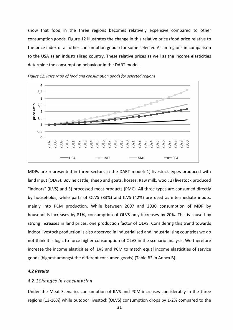
show that food in the three regions becomes relatively expensive compared to other

consumption goods. Figure 12 illustrates the change in this relative price (food price relative to

the price index of all other consumption goods) for some selected Asian regions in comparison

to the USA as an industrialised country. These relative prices as well as the income elasticities

determine the consumption behaviour in the DART model.

Figure 12: Price ratio of food and consumption goods for selected regions

MDPs are represented in three sectors in the DART model: 1) livestock types produced with

land input (OLVS): Bovine cattle, sheep and goats, horses; Raw milk, wool; 2) livestock produced

“indoors” (ILVS) and 3) processed meat products (PMC). All three types are consumed directly

by households, while parts of OLVS (33%) and ILVS (42%) are used as intermediate inputs,

mainly into PCM production. While between 2007 and 2030 consumption of MDP by

households increases by 81%, consumption of OLVS only increases by 20%. This is caused by

strong increases in land prices, one production factor of OLVS. Considering this trend towards

indoor livestock production is also abserved in industrialised and industrialising countries we do

not think it is logic to force higher consumption of OLVS in the scenario analysis. We therefore

increase the income elasticities of ILVS and PCM to match equal income elasticities of service

goods (highest amongst the different consumed goods) (Table B2 in Annex B).

4.2 Results

4.2.1Changes in consumption

Under the Meat Scenario, consumption of ILVS and PCM increases considerably in the three

regions (13-16%) while outdoor livestock (OLVS) consumption drops by 1-2% compared to the

0

0,5

1

1,5

2

2,5

3

3,5

4

20

07

20

08

20

09

20

10

20

11

20

12

20

13

20

14

20

15

20

16

20

17

20

18

20

19

20

20

20

21

20

22

20

23

20

24

20

25

20

26

20

27

20

28

20

29

20

30

pri

ce r

atio

USA IND MAI SEA

32

Baseline Scenario in 2030 (Figure 13). The share of ILVS and PCM on total consumption

increases at the costs of energy, manufacturing and service goods. Within the food basket, the

share of non-meat food (VEG) decreases by 0.3-0.5%.

Figure 13: Share of food sectors on total food consumption in IND, MAI and SEA

Comparing consumption of ILVS and PCM in 2030 under the two scenarios, results show that

ILVS and PCM consumption of Asian households increases by about 4.2%, causing small

consumption reductions in all other regions. Globally, consumption of ILVS and PCM increases

by 0.9%. The impact on global and regional production and prices of agricultural goods and

biofuels is discussed in the following section.

4.2.2 Changes in prices and quantities

Comparing results of the scenarios in 2030 these changes in demand cause slight increases in

global production of ILVS (+0.7%), soyoil and soy meal (+0.7%), and PCM 0.5%. Accordingly,

global feedstuff prices (Palm meal 2.8%, Soybean meal +0.2%) increase while prices of

vegetable oils fall (Soyoil -0.7%).

Regionally, considerable changes in production, trade and prices for feedstuff as well as ILVS

and PCM occur. For the sake of clarity, we take the region SEA as an example to illustrate a)

regional changes in production, b) changes in relative prices of processed food and

consumption goods, and c) changes in trade flows.

0%

20%

40%

60%

80%

100%

Baseline Meat Scenario Baseline Meat Scenario Baseline Meat Scenario

IND MAI SEA

OLVS

ILVS

PCM

VEG

+13%

+15% +16%

33

In 2007, livestock in SEA is mainly produced from LAB (31%), FOD (21%), and soymeal (8.8%).

From 2007-2030, livestock production 2.2-folds, causing soymeal production to 2.6-fold under

the baseline scenario. When implementing the Meat Scenario, the soybean meal and oil

production increase by 5.9% compared to the baseline scenario in 2030. Meat production

increase by 8 and 9.1% respectively (see Table 6).

The increased demand for soybean meal causes soyoil prices to decrease, since they are

produced in a jointed production process. Crops are only used to a very small share for

livestock production; hence there are no significant quantity or price changes in these sectors.

Table 6: Changes in production, prices and trade comparing the scenarios in 2030 in SEA

Q Change P Change Change of net

exported goods Change of net

imported goods

PDR 0.0% 0.3% -0.3%

SOY 4.8% 0.3% 5.0%

AGR -0.1% 0.2% -4.6%

SOYmeal 6.0% 0.7%

7.4%

SOYoil 6.0% -2.7%

-0.7%

ILVS 8.0% 0.2% 9.6%

FOD -0.1% 0.1% 3.0%

PCM 9.1% 0.2% 19.1%

The increased demand for livestock and feedstuff is not only met by increased domestic

production, but also less exports and more imports. Highes trade flows occur in the FOD sector

which increases by 3.0% under the Meat Scenario. Major import sources are GBR, FRA and ANZ,

while main destination of net exports is MAI. Table 6 illustrates a decreases of net exports for

PDR and AGR, while net imports of livestock and feedstuff sectors increase. The two major

sources of net imports of livestock and processed meat in 2030 to SEA are USA and ANZ.

Comparing trade flows in 2030 under the two scenarios, result show that livestock net imports

to SEA from the USA increase by 9.7%, while total net exports of the USA only increase by 0.4%.

An increase in US-american exports to SEA (and also IND (+17.1%) and MAI (+18.6%)) is

compensated by less exports to almost all other regions (with CHN being to main importer of

US livestock). However, this effect is very small since exports to SEA only make up 6.5% (6%

under Baseline scenario) of total net exports.

34

More than half of net imports of soybeans to SEA stem from BRA, about 25% from USA.

Soybean imports from the USA to SEA increase by about 4.7%, from BRA by about 5.1%. Again,

the higher demand from SEA (and MAI) is compensated by less exports to other regions. Soyoil,

which net imports decrease under the Meat Scenario is imported mainly from PAO and BRA.

Since demand for soybean meal as feedstuff increases under the Meat Scenario, more soyoil is

produced in countries with higher meat production and imports of soyoil decreases.

The consideration of by-products from biofuel production has been assessed to have significant

impact on land use and prices in the agricultural sector (Taheripour et al. 2010). An important

assumption to be made is the degree of substitution between by-products of biofuel

production and crops used for feedstuff in livestock production. Since there is little literature on

which value for elasticity of substitution to take, we test the sensitivity of this parameter in the

following sensitivity analysis.

4.2.3 Sensitivity analysis

In the baseline scenario, the input share of wheat, soymeal and DDGS in livestock production

increases between 2007 and 2030. This is due to relatively low prices for wheat and an

increasing production of biofuels. Note that in all scenarios biofuel quotas are implemented

causing production increases of biodiesel and bioethanol in several countries (see section 4.1).

In the production of biofuels by-products are produced which can be used for livestock

production by substituting other feedstuff (see Figure 8). When reducing the elasticity of

substitution of feedstuff in the production function of livestock from 2 to 0.5 (LVS 05 Scenario

in Table 7) 15% less soymeal is used for livestock production while more AGR (9.8%), MZE

(9.6%) and PDR (53.1%) are used. Note that the use of PDR increases from a low absolute value.

An opposite effect is caused when increasing the elasticity of substitution to 4 (LVS 4 Scenario

in Table 7). Table 7 illustrates price and quantity changes in 2030 compared to baseline. When

decreasing the elasticity of substitution for feedstuff (LVS 05 Scenario), we see different price

effects of crops depending on the share of the crop that is used in biofuel and/or livestock

production. Annual crops have one land price in our model. Therefore, since less soymeal is

used in livestock production, soy bean production decreases by 7.6% causing land prices to

decrease in major soybean producing countries (USA, BRA, PAO) while land prices increase in

almost all other regions. The share of PDR used for livestock production increases under the

LVS 05 scenario, causing the price for PDR to increase considerably. The reduced ability to

35

substitute feedstuff in livestock production causes prices for by-products and wheat to fall

while vegetable oils demanded for biodiesel production become more expensive. Increasing

the elasticity of substitution to 4 causes the opposite effect. In summary, the sensitivity analysis

shows that model results are highly influenced by the extend of the substitution of feedstuff,

indicating that it is an important driver of price differences among studies.

Table 7: Global Quantity and Price Changes 2030 compared to Baseline Scenario in %

Quantity Change Price Change

Meat Scenario

LVS 05 Scenario

LVS 4 Scenario

Meat Scenario

LVS 05 Scenario

LVS 4 Scenario

MZE 0.0 2.0 -1.9 0.1 -0.3 0.1

WHT 0.0 -2.7 1.8 0.1 -0.1 0.0

SOY 0.4 -7.6 6.3 0.1 -0.5 0.3

AGR 0.0 0.0 -0.2 0.1 -0.2 0.0

PDR 0.0 2.7 -1.2 0.1 10.5 -4.0

RSDoil -0.1 -1.1 0.1 -0.4 0.7 -1.6

RSDmeal -0.3 -3.0 1.8 0.3 -8.3 5.9

SOYoil 0.7 -11.1 9.4 -0.7 18.5 -10.7

SOYmeal 0.5 -14.7 12.6 0.2 -6.3 3.5

DDGSm 0.0 -1.4 0.1 0.1 -55.7 17.6

BETH 0.0 -1.3 0.5 0.1 9.6 -3.5

BDIE 0.1 -1.3 2.3 -0.2 8.5 -5.1

5. Summary and Conclusions

We have discussed the current approaches for modelling land use, land use change and the

markets for the different forms of agricultural products and their further conversion into

consumption goods. It turns out that the particular modelling approach chosen strongly

influences the results of the numerical model. We therefore present in detail the assumptions

and structural equations for modelling the value chain from agricultural raw materials to the

many final consumption goods which use agricultural products as an input. The new DART-BIO

model allows us to model the interplay of food, feed, and biofuels in a more transparent and

realistic way.

The often expected drastic increase in meat consumption in mainly Asian countries and the

subsequent threat of large scale land use change, a loss of ecosystem services, and increasing

36

food prices leading to a loss in food security especially in poor countries has been subject to our

scenario analysis. We find that such fears are exaggerated. Even strong growth in Asian

countries and under the assumption of very high income elasticities for meat products the

share of meat consumption will by far fall short of comparable numbers in regions like the

North America or Europe. The main reason being that the price of meat products relative to

those of other consumption goods rises thus leading to a substitution away from meat

consumption. The interregional trade will alleviate the shortages in many regions and the trade

in agricultural products will further increase.

An important result of the detailed modelling of agricultural value chains in the DART-BIO

model concerns the role of the elasticity of substitution between inputs in the manufacturing

activities that use biomass. Especially the results on the price effects of agricultural policies

depend crucially on the substitutability of inputs in the livestock sector.

References

Abler, D.G. (2000): Elasticities of Substitution and Factor Supply in Canadian, Mexican and US Agriculture. Report to the Policy Evaluation Matrix (PEM) Project Group, OECD, Paris.

Al-Riffai, P., Dimaranan, B., D. Laborde (2010): Global Trade and Environmental Impact Study of the EU Biofuels Mandate. International Food Policy Institute (IFPRI), Final Report, March 2010. URL: http://www.ifpri.org/sites/default/files/publications/biofuelsreportec.pdf.

Avetisyan, M., Baldos, U., T.W. Hertel (2010): Development of the GTAP Version 7 Land Use Data Base. GTAP Research Memorandum 19, updated 2011, Center for Global Trade Analysis, Department of Agricultural Economics, Purdue University.

Baldos, U.L.C., T.W. Hertel (2012): Development of a GTAP 8 Land Use and Land Cover Data Base for Years 2004 and 2007. GTAP Research Memorandum No. 23,September 2012. URL: https://www.gtap.agecon.purdue.edu/resources/res_display.asp?RecordID=3967 .

Banse, M., Van Meijl, H., Tabeau, A., G. Woltjer (2008): Will EU biofuel policies affect global agricultural markets?. European Review of Agricultural Economics 35(2), 117-141.

Beurskens, L.W.M., Hekkenberg, M., P. Vethman (2011): Renewable Energy Projections as Published in the National Renewable Energy Action Plans of the European Member States. Covering all 27 EU Member States with updates for 20 Member States. European Environmental Agency, ECN-E—10-069, 28 November 2011. URL: http://ec.europa.eu/energy/renewables/action_plan_en.htm.

Bouët, A., Dimaranan, B. V., H. Valin (2010): Modeling the global trade and environmental impacts of biofuel policies. IFPRI Discussion Paper (01018), International Food Policy Research Institute.

Dixon, P.B., Osborne, S., M.T. Rimmer (2007): The economy-wide effects in the United States of replacing crude petroleum with biomass. Energy and Environment 18 (6), 709–722.

Ecofys-Agra CEAS-Chalmers University-IIASA-Winrock (2011): Biofuels Baseline 2008. Tender No. TREN/D1/458/2009.

ERS-USDA (2010): Market Issues and Prospects for U.S. Distillers’ Grains: Supply, Use, and Price Relationships. FDS-10k-01, Economic Research Service/USDA.

37

FAO (Food and Agricultural Organization of the United Nations) (2011): Mapping Supply and Demand for animal-sourced foods to 2030. FAO Animal Production and Health, Working Paper 2, Rome.

FAOSTAT (current issues): Food and Agriculture Organization Corporate Statistical Database, http://faostat.fao.org/.

F.O.Licht (2008): F.O.Licht's World Ethanol and Biofuels Report, Vol.6, No.16, 25.04.2008.

F.O.Licht (2010): F.O.Licht's World Ethanol and Biofuels Report, Vol.9, No.1, 10.09.2010.

F.O.Licht (2011): F.O.Licht's World Ethanol and Biofuels Report, Vol.9, No.10, 01.02.2011.

Foley, J.A., M.H. Costa, C. Delire, N. Ramankutty, P. Snyder (2003): Green Surprise? How terrestrial ecosystems could affect earth’s climate. Frontiers in Ecology and the Environment, 1 (1), 38-44.

Golub A., T. Hertel, B. Sohngen (2011): Land Use Modelling in Recursively-Dynamic GTAP Framework. In: Hertel,T., Rose, S., Tol, R. Economic Analysis of Land Use in Global Climate Change Policy, Routledge Chapman & Hall, 235-278.

Gouel, C., T.W. Hertel (2006): Introducing Forest Access Cost Functions into a General Equilibrium Model. GTAP Research Memorandum No. 08,. Center for Global Trade Analysis, Department of Agricultural Economics, Purdue University. URL: https://www.gtap.agecon.purdue.edu/resources/download/2899.pdf.

Haxeltine, A., C. Prentice (1996): BIOME3: An Equilibrium Terrestrial Biosphere Model Based on Ecophysiological Constraints, Resource Availability, and Competition Among Plant Functional Types. Global Biogeochemical Cycles 10(4), 693-709.

Hertel, T., Golub, A., Jones, A., OHare, M., Plevin, R., D. Kammen (2010): Effects of US Maize Ethanol on Global Land Use and Greenhouse Gas Emissions: Estimating Market-mediated Responses. BioScience 60(3), 223-231.

Hilderink, H.B.M. (2000): PHOENIX pluss: the population user support system version 1.0, URL: www.mnp.nl/phoenix.

Horridge, M. (2005): SplitCom - Programs to Disaggregate a GTAP Sector. Centre of Policy Studies, Monash University, Melbourne, Australia.

IEA (International Energy Agency) (2008): Annual Energy Outook 2008 – With Projections to 2030. Energy Information Administration, Office of Integrated Analysis and Forecasting, U.S. Department of Energy.

IEA (International Energy Agency) (2009) A Global Overview of Vegetable Oils, with Reference to Biodiesel. A report of the IEA Bioenergy task 40.

IEA (International Energy Agency) (2012) Energy Prices and Taxes – Quarterly Statistics. International Energy Agency, Fourth Quarter 2012.

Klepper, G., Peterson S., K. Springer (2003): DART97: A Description of the Multi-regional, Multi-sectoral Trade Model for the Analysis of Climate Policies. Kiel Working Paper 1149, Institute for the World Economy, Kiel.

Klepper, G., S. Peterson (2006a): Emissions Trading, CDM, JI and More — The Climate Strategy of the EU. The Energy Journal 27(2), 1-26.

Klepper, G., S. Peterson (2006b): Marginal Abatement Cost Curves in General Equilibrium:The Influence of World Energy Prices. Resource and Energy Economics 28(1),1-23.

Kretschmer, B., Narita, D., S. Peterson (2009): The Economic Effects of the EU Biofuel Target. Energy Economics 31, 285-294.

Kretschmer, B., S. Peterson (2010): Integrating bioenergy into computable general equilibrium models – A survey. Energy Economics 32(3), 673-686.

38

Laborde, D. (2011): Assessing the Land Use Change Consequences of European Biofuel Policies. Final Report prepared for the European Commission DG Trade, Implementing Framework Contract No TRADE/07/A2. URL http://trade.ec.europa.eu/doclib/docs/2011/october/tradoc_148289.pdf

Laborde D., H. Valin (2012): Modelling Land Use Changes in a Global CGE: Assessing the EU biofuel mandates with the MIRAGE-BioF model. Climate Change Economics 3 (3) 1250017.

Lee, H.L., Hertel, T., Sohngen, B., N. Ramankutty (2005): Towards An Integrated Land Use Database for Assessing the Potential for Greenhouse Gas Mitigation. GTAP Technical Paper No. 25,. Center for Global Trade Analysis, Department of Agricultural Economics, Purdue University. URL: https://www.gtap.agecon.purdue.edu/resources/download/2375.pdf.

Lee H.-L., Hertel, T., Rose, S., M. Avetisyan (2011): An Integrated Global Land Use Data Base for CGE Analysis of Climate Policy Options. In: Hertel,T., Rose, S., Tol, R. Economic Analysis of Land Use in Global Climate Change Policy, Routledge Chapman & Hall, 72-88.

Monfreda, C., Ramankutty, N., T.W. Hertel (2011): Global agriculture land use data for climate change analysis. In: Hertel,T., Rose, S., Tol, R. Economic Analysis of Land Use in Global Climate Change Policy, Routledge Chapman & Hall, 33-48.

Monfreda, C., Ramankutt, N., J.A. Foley (2008): Farming the Planet. Part 2: The Geographic Distribution of Crop Areas and Yields in the Year 2000. Glob. Biogeochem. Cycles, doi:10.1029/2007GB002947.

Narayanan, G., Badri, A. A., R. McDougall (Eds.) (2012): Global Trade, Assistance, and Production: The GTAP 8 Data Base, Center for Global Trade Analysis, Purdue University, West Lafayette, USA.

OECD-IEA (Organisation for Economic Co-operation and Development – International Energy Agency) (2006): The energy situation in Brazil: An overview. Office of Global Energy Dialogue (OGED), paper prepared for the Standing Group on the Global Energy Dialogue.

OECD-IEA (2010): Sustainable Production of Second-General Biofuels: Potential and Perspectives in Major Economics and Developing Countries. IEA, Paris.

OECD-FAO (Organisation for Economic Co-operation and Development – Food and Agriculture Organization) (2011): OECD-FAO Agricultural Outlook 2011-2020. OECD, Paris.

OECD-FAO (2012): OECD-FAO Agricultural Outlook 2012-2021. OECD, Paris.

Ramankutty, N., Evan, A., Monfreda, C., J.A. Foley (2008): Farming the Planet. Part 1: The Geographic Distribution of Global Agricultural Lands in the Year 2000. Glob. Biogeochem. Cycles, doi:10.1029/2007GB002952.

Ramankutty, N., J.A. Foley (1998): Characterizing patterns of global land use: An analysis of global croplands data. Global Biochemical Cycles 12(4), 667-685.

Ramankutty, N., J.A. Foley (1999): Estimating Historical Changes in Global Land Cover: Croplands from 1700 to 1992. Global Biogeochemical Cycles, 13, 997-1027.

Rose, S.K., Avetisyan, M., T.W. Hertel (2010): Development of the Preliminary Version 7 Non-CO2 GHG Emissions Dataset. GTAP Research Memorandum No.17.

Salhofer, K. (2000): Elasticities of Substitution and Factor Supply Elasticities in European Agriculture: A Review of Past Studies. Diskussionspapier Nr. 83-W-2000. Institut für Wirtschaft, Politik und Recht, Universität für Bodenkultur, Wien, Austria.

Sohngen, B., Mendelsohn, R., R. Sedjo (1999): Forest Management, Conservation, and Global Timber Markets. American Journal of Agricultural Economics 81, 1-13.

Sohngen, B., C. & Tennity (2004): Country Specific Global Forest Data Set V.1. memo. Department of Agricultural, Environmental, and Development Economics, Ohio State University, Columbus, OH 43210, U.S.A.

39

Sohngen, B., Tennity, C., Hnytka, M., K. Meeusen (2011): Global Forestry Data for the Economic Modeling of Land Use. In: Hertel,T., Rose, S., Tol, R. Economic Analysis of Land Use in Global Climate Change Policy, Routledge Chapman & Hall, 49-71.

Sohngen, B., R. Mendelsohn (2003): An Optimal Control Model of Forest Carbon Sequestration. American Journal of Agricultural Economics 85(2): 448-457.

Sohngen, B., R. Mendelsohn (2007): A Sensitivity Analysis of Carbon Sequestration. In Human-Induced Climate Change: An Interdisciplinary Assessment. Edited by M. Schlesinger et al. Cambridge: Cambridge University Press, 228-235.

Springer, K. (1998): The DART General Equilibrium Model: A Technical Description. Kiel Working Paper No. 883, Kiel Institute for the World Economy, Kiel.

Springer, K. (2002): Climate Policy in a Globalizing World: A CGE Model with Capital Mobility and Trade. Kieler Studien. Springer, Berlin.

Stone, R. (1954): Linear Expenditure Systems and Demand Analysis: An Application to the Pattern of British Demand. Economic Journal 64, 511-527.

Taheripour, F., Hertel, T. W., Tyner, W. E., Beckman, J. F., D.K. Birur (2010): Biofuels and their by-products: Global economic and environmental implications. Biomass and Bioenergy 34(3), 278-289.

United Nations, Department of Economic and Social Affairs, Population Division, Population Estimates and Projections Section (2010).

USDA (United States Department of Agriculture) (2012): Oilseeds: World Markets and Trade. Foreign Agricultural Services, circular series FOP 12-12.

USDA/FAS (United States Department of Agriculture/Foreign Agricultural Service) (2010): Brazil – biofuels annual – 2007. Global Agricultural Information Network Report BR10006.

UNICA (Sugarcane Industry Association) (2013): Preço final de faturamento do ATR por produto - Modelo Consecana-SP - valores médios para o Estado de São Paulo, UNICA, Departamento de economia y estatistica.

Weitzel, M., M. Hübler, S. Peterson (2012): Fair, Optimal or Detrimental? Environmental vs. Strategic Use of Carbon-based Border Measures. Energy Economics 34(2), 198-207.

40

Annex

Annex A: DART-BIO database (new sectors)

Figure A1. Regional production of maize and other cereal grains in DART (million USD)

Maize is the dominant type of cereal grain produced in the USA, China, Malaysia & Indonesia

and all Latin-American countries. Other cereals like burley dominate the production in Russia,

the Middle East and in most of the African countries. In India is particularly important the millet

and sorghum production.

Source: DART-BIO, based on FAO data.

Note: Germany (DEU); UK, Ireland (GBR); France (FRA); Finland, Sweden, Denmark (SCA); Belgium, Netherlands, Luxemburg (BEN); Spain, Portugal, Italy, Greece, Malta, Cyprus (MED); Rest of European Union (REU); USA (USA); Canada (CAN); Australia, New Zealand (ANZ); Japan (JPN); Russia (RUS); Rest of Former Soviet Union and Europe (FSU); Brazil (BRA); Paraguay, Argentina, Uruguay, Chile (PAO); Rest of Latin America (LAM); China (CHN); India (IND); Malaysia, Indonesia (MAI); South East Asia (SEA); Middle East, North Africa (MEA); Sub-Saharan Africa (AFR); Rest of the World (ROW).

0

10,000

20,000

30,000

40,000

50,000

60,000

DE

U

GB

R

FRA

SCA

BE

N

ME

D

RE

U

USA

CA

N

AN

Z

JPN

RU

S

FSU

BR

A

PA

O

LAM

CH

N

IND

MA

I

SEA

ME

A

AFR

RO

W

Maize (MZE) Other cereals (GRON)

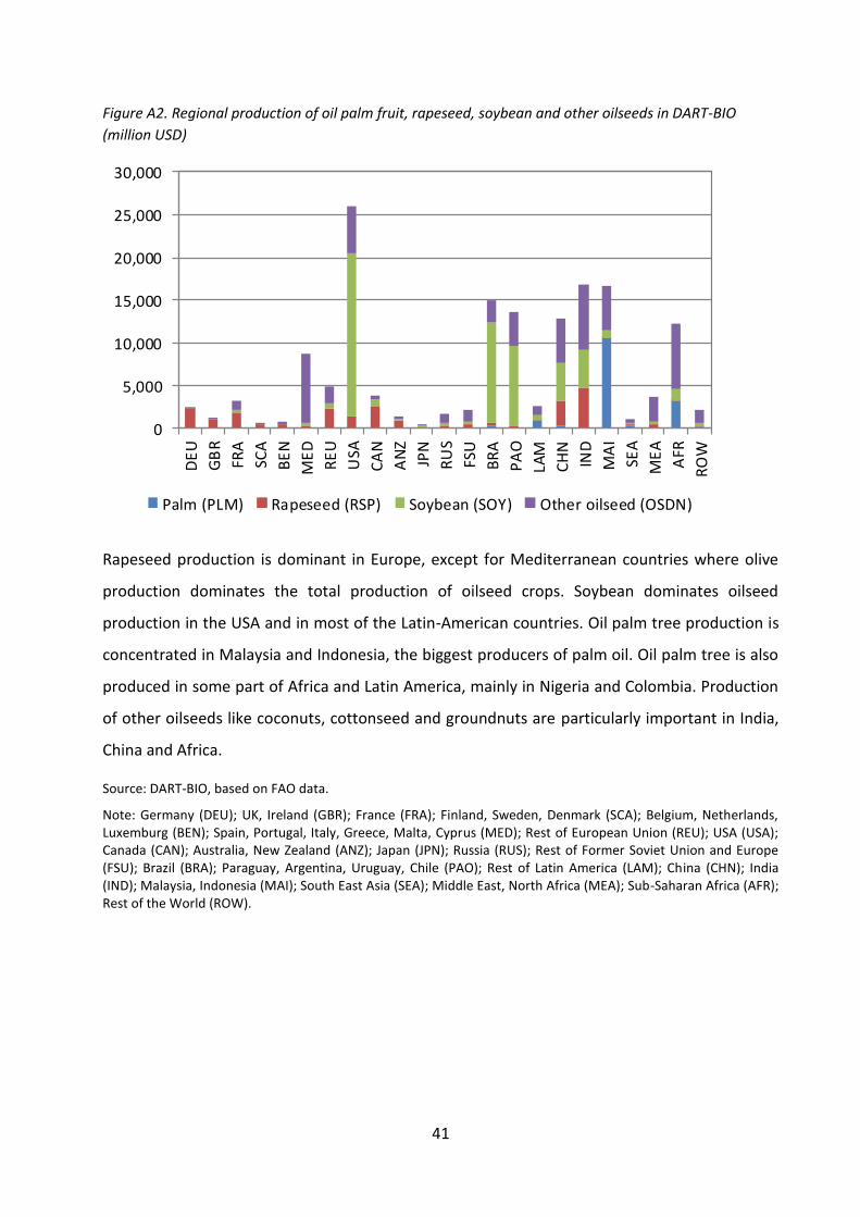
41

Figure A2. Regional production of oil palm fruit, rapeseed, soybean and other oilseeds in DART-BIO

(million USD)

Rapeseed production is dominant in Europe, except for Mediterranean countries where olive

production dominates the total production of oilseed crops. Soybean dominates oilseed

production in the USA and in most of the Latin-American countries. Oil palm tree production is

concentrated in Malaysia and Indonesia, the biggest producers of palm oil. Oil palm tree is also

produced in some part of Africa and Latin America, mainly in Nigeria and Colombia. Production

of other oilseeds like coconuts, cottonseed and groundnuts are particularly important in India,

China and Africa.

Source: DART-BIO, based on FAO data.

Note: Germany (DEU); UK, Ireland (GBR); France (FRA); Finland, Sweden, Denmark (SCA); Belgium, Netherlands, Luxemburg (BEN); Spain, Portugal, Italy, Greece, Malta, Cyprus (MED); Rest of European Union (REU); USA (USA); Canada (CAN); Australia, New Zealand (ANZ); Japan (JPN); Russia (RUS); Rest of Former Soviet Union and Europe (FSU); Brazil (BRA); Paraguay, Argentina, Uruguay, Chile (PAO); Rest of Latin America (LAM); China (CHN); India (IND); Malaysia, Indonesia (MAI); South East Asia (SEA); Middle East, North Africa (MEA); Sub-Saharan Africa (AFR); Rest of the World (ROW).

0

5,000

10,000

15,000

20,000

25,000

30,000D

EU

GB

R

FRA

SCA

BE

N

ME

D

RE

U

USA

CA

N

AN

Z

JPN

RU

S

FSU

BR

A

PA

O

LAM

CH

N

IND

MA

I

SEA

ME

A

AFR

RO

W

Palm (PLM) Rapeseed (RSP) Soybean (SOY) Other oilseed (OSDN)

42

Figure A3. Regional production of oils and meals from palm, rapeseed, soybean and other oilseeds as

well as other vegetable oils in DART-BIO (million USD)

Globally, the vegetable oil market is dominated by soy oil, followed by palm oil and rapeseed

oil. Soy meal is the largest produced oil meal; the global production of soy meal is much more

valuable than soy oil. Regional production patterns of vegetable oils are similar to the regional

oilseed production (see Figure A2). Other vegetable oils (VOLN) are important in the

Mediterranean region (olive oil) and in India, China and Africa (coconuts, cottonseed and

groundnuts).

Source: DART-BIO, based on FAO data, IEA (2009) and USDA (2012).

Note: Germany (DEU); UK, Ireland (GBR); France (FRA); Finland, Sweden, Denmark (SCA); Belgium, Netherlands, Luxemburg (BEN); Spain, Portugal, Italy, Greece, Malta, Cyprus (MED); Rest of European Union (REU); USA (USA); Canada (CAN); Australia, New Zealand (ANZ); Japan (JPN); Russia (RUS); Rest of Former Soviet Union and Europe (FSU); Brazil (BRA); Paraguay, Argentina, Uruguay, Chile (PAO); Rest of Latin America (LAM); China (CHN); India (IND); Malaysia, Indonesia (MAI); South East Asia (SEA); Middle East, North Africa (MEA); Sub-Saharan Africa (AFR); Rest of the World (ROW).

0

10,000

20,000

30,000

40,000

50,000

60,000

70,000

80,000

DE

U

GB

R

FRA

SCA

BE

N

ME

D

RE

U

USA

CA

N

AN

Z

JPN

RU

S

FSU

BR

A

PA

O

LAM

CH

N

IND

MA

I

SEA

ME

A

AFR

RO

W

PLMoil PLMmeal RSDoil RSDmeal SOYoil

SOYmeal OSDNoil OSDNmeal VOLN

43

Figure A4. Regional production of motor gasoline, motor diesel and other oil and coal products in DART-

BIO (million USD)

At the global level, more motor gasoline is produced than motor diesel. However, motor diesel

dominates production in Europe, India and South East Asia (compared with motor gasoline).

The production of other oil and coal products (OIL) is significant in all regions, representing

around 50% to 85% of all oil and cold products.

Source: DART-BIO, based on UNSD data, COMTRADE data and IEA (2012).

Note: Germany (DEU); UK, Ireland (GBR); France (FRA); Finland, Sweden, Denmark (SCA); Belgium, Netherlands, Luxemburg (BEN); Spain, Portugal, Italy, Greece, Malta, Cyprus (MED); Rest of European Union (REU); USA (USA); Canada (CAN); Australia, New Zealand (ANZ); Japan (JPN); Russia (RUS); Rest of Former Soviet Union and Europe (FSU); Brazil (BRA); Paraguay, Argentina, Uruguay, Chile (PAO); Rest of Latin America (LAM); China (CHN); India (IND); Malaysia, Indonesia (MAI); South East Asia (SEA); Middle East, North Africa (MEA); Sub-Saharan Africa (AFR); Rest of the World (ROW).

0

100,000

200,000

300,000

400,000

500,000

600,000D

EU

GB

R

FRA

SCA

BE

N

ME

D

RE

U

USA

CA

N

AN

Z

JPN

RU

S

FSU

BR

A

PA

O

LAM

CH

N

IND

MA

I

SEA

ME

A

AFR

RO

W

Motor gasoline (MGAS) Motor diesel (MDIE) Other oil and coal prodts. (OIL)

44

Annex B:

Table B1: Elasticites of transformation

DEU GBR FRA SCA BEN MED REU USA CAN ANZ JPN RUS FSU BRA PAO LAM CHN IND MAI SEA MEA AFR ROW

CET1 0.05 0.05 0.05 0.05 0.05 0.05 0.05 0.1 0.05 0.05 0.05 0.05 0.05 0.05 0.05 0.1 0.05 0.05 0.05 0.05 0.05 0.05 0.05

CET2 0.21 0.21 0.21 0.21 0.21 0.21 0.21 0.15 0.14 0.17 0.11 0.21 0.21 0.21 0.21 0.11 0.21 0.21 0.21 0.21 0.15 0.21 0.11

CET3 0.22 0.22 0.22 0.22 0.22 0.22 0.22 0.32 0.32 0.3 0.15 0.22 0.22 0.22 0.22 0.3 0.22 0.22 0.22 0.22 0.24 0.24 0.15

Source: Abler 2000 and Salhofer 2000 used in the OECD’s PEM model; The OECD model only covers developed countries plus Mexico, Turkey, and South Korea. Therefore, we had to assume certain similarities for several countries.

Table B2: Income elasticities

DEU GBR FRA SCA BEN MED REU USA CAN ANZ JPN RUS FSU BRA PAO LAM CHN IND MAI SEA MEA AFR ROW

PDR 0.36 0.21 0.17 0.27 0.56 0.56 0.72 0.43 0.68 0.61

WHT 0.02 0.02 0.02 0.02 0.02 0.03 0.13 0.03 0.2 0.38 0.21 0.17 0.33 0.55 0.56 0.62 0.43 0.6 0.4

MZE 0.02 0.02 0.02 0.02 0.02 0.03 0.15 0.01 0.02 0.02 0.2 0.39 0.21 0.24 0.28 0.54 0.56 0.53 0.62 0.41 0.64 0.41

GRON 0.02 0.02 0.02 0.02 0.02 0.03 0.13 0.02 0.02 0.02 0.2 0.38 0.21 0.19 0.26 0.55 0.56 0.53 0.63 0.4 0.67 0.34

PLM 0.38 0.53 0.41 0.67 0.5

RSD 0.03 0.02 0.03 0.11 0.02 0.2 0.32 0.56 0.34 0.47 0.05

SOY 0.03 0.02 0.04 0.11 0.02 0.2 0.25 0.24 0.26 0.03 0.56 0.53 0.43 0.38 0.68 0.08

OSDN 0.02 0.03 0.12 0.02 0.2 0.29 0.36 0.56 0.53 0.58 0.41 0.68 0.23

C_B 0.02 0.02 0.02 0.02 0.02 0.03 0.25 0.01 0.02 0.02 0.4 0.17 0.19 0.56 0.3 0.64 0.53 0.45 0.3

OLVS 0.86 0.89 0.87 0.88 0.92 0.86 0.77 0.9 0.88 0.87 0.85 0.7 0.77 0.68 0.73 0.7 0.82 0.92 0.81 1.06 0.8 1.05 0.93

ILVS 0.86 0.89 0.87 0.88 0.87 0.85 0.77 0.9 0.87 0.86 0.85 0.7 0.79 0.66 0.67 0.7 0.81 0.92 0.79 0.9 0.79 0.97 0.87

AGR 0.04 0.02 0.03 0.02 0.03 0.04 0.13 0.01 0.08 0.04 0.02 0.21 0.43 0.21 0.28 0.3 0.54 0.56 0.51 0.54 0.43 0.66 0.3

FRS 1.02 1.02 1.02 1.02 1.02 1.03 1.07 1.01 1.02 1.02 1.03 1.13 1.19 1.07 1.11 1.1 1.06 1.06 1.09 1.01 1.13 1.11 1.04

PLMoil 0.91 0.9 0.87 0.77 0.88 0.87 0.72 0.68 0.74 0.71 0.72 0.66 0.71 0.71 0.76 0.77 0.74

RSDoil 0.88 0.91 0.89 0.89 0.9 0.87 0.78 0.91 0.89 0.88 0.87 0.71 0.7 0.72 0.71 0.66 0.66 0.74 0.72 0.75 0.78

SOYoil 0.88 0.91 0.89 0.9 0.89 0.87 0.77 0.89 0.87 0.87 0.72 0.72 0.68 0.72 0.72 0.71 0.66 0.71 0.72 0.73 0.72 0.79

OSDNoil 0.88 0.91 0.89 0.9 0.9 0.87 0.77 0.88 0.72 0.71 0.68 0.69 0.72 0.71 0.66 0.71 0.7 0.75 0.7 0.78

VOLN 0.88 0.91 0.89 0.9 0.89 0.87 0.77 0.91 0.89 0.87 0.87 0.72 0.73 0.68 0.71 0.72 0.71 0.66 0.71 0.73 0.75 0.75 0.76

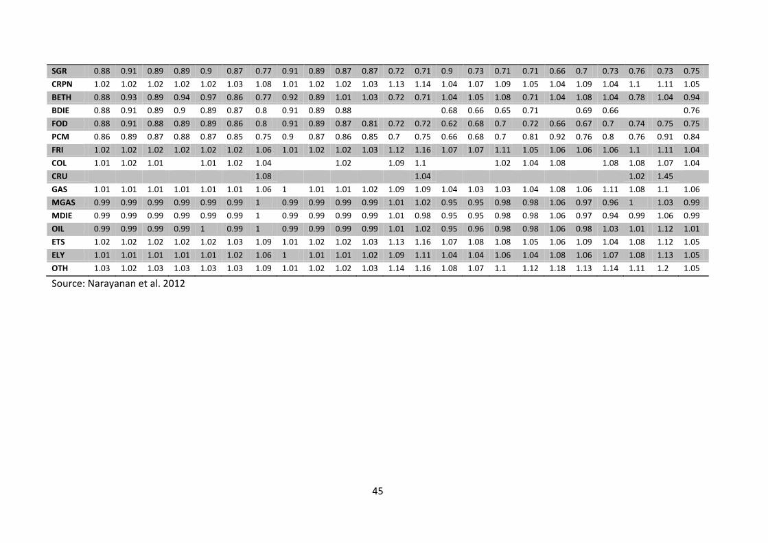
45

SGR 0.88 0.91 0.89 0.89 0.9 0.87 0.77 0.91 0.89 0.87 0.87 0.72 0.71 0.9 0.73 0.71 0.71 0.66 0.7 0.73 0.76 0.73 0.75

CRPN 1.02 1.02 1.02 1.02 1.02 1.03 1.08 1.01 1.02 1.02 1.03 1.13 1.14 1.04 1.07 1.09 1.05 1.04 1.09 1.04 1.1 1.11 1.05

BETH 0.88 0.93 0.89 0.94 0.97 0.86 0.77 0.92 0.89 1.01 1.03 0.72 0.71 1.04 1.05 1.08 0.71 1.04 1.08 1.04 0.78 1.04 0.94

BDIE 0.88 0.91 0.89 0.9 0.89 0.87 0.8 0.91 0.89 0.88 0.68 0.66 0.65 0.71 0.69 0.66 0.76

FOD 0.88 0.91 0.88 0.89 0.89 0.86 0.8 0.91 0.89 0.87 0.81 0.72 0.72 0.62 0.68 0.7 0.72 0.66 0.67 0.7 0.74 0.75 0.75

PCM 0.86 0.89 0.87 0.88 0.87 0.85 0.75 0.9 0.87 0.86 0.85 0.7 0.75 0.66 0.68 0.7 0.81 0.92 0.76 0.8 0.76 0.91 0.84

FRI 1.02 1.02 1.02 1.02 1.02 1.02 1.06 1.01 1.02 1.02 1.03 1.12 1.16 1.07 1.07 1.11 1.05 1.06 1.06 1.06 1.1 1.11 1.04

COL 1.01 1.02 1.01 1.01 1.02 1.04 1.02 1.09 1.1 1.02 1.04 1.08 1.08 1.08 1.07 1.04

CRU 1.08 1.04 1.02 1.45

GAS 1.01 1.01 1.01 1.01 1.01 1.01 1.06 1 1.01 1.01 1.02 1.09 1.09 1.04 1.03 1.03 1.04 1.08 1.06 1.11 1.08 1.1 1.06

MGAS 0.99 0.99 0.99 0.99 0.99 0.99 1 0.99 0.99 0.99 0.99 1.01 1.02 0.95 0.95 0.98 0.98 1.06 0.97 0.96 1 1.03 0.99

MDIE 0.99 0.99 0.99 0.99 0.99 0.99 1 0.99 0.99 0.99 0.99 1.01 0.98 0.95 0.95 0.98 0.98 1.06 0.97 0.94 0.99 1.06 0.99

OIL 0.99 0.99 0.99 0.99 1 0.99 1 0.99 0.99 0.99 0.99 1.01 1.02 0.95 0.96 0.98 0.98 1.06 0.98 1.03 1.01 1.12 1.01

ETS 1.02 1.02 1.02 1.02 1.02 1.03 1.09 1.01 1.02 1.02 1.03 1.13 1.16 1.07 1.08 1.08 1.05 1.06 1.09 1.04 1.08 1.12 1.05

ELY 1.01 1.01 1.01 1.01 1.01 1.02 1.06 1 1.01 1.01 1.02 1.09 1.11 1.04 1.04 1.06 1.04 1.08 1.06 1.07 1.08 1.13 1.05

OTH 1.03 1.02 1.03 1.03 1.03 1.03 1.09 1.01 1.02 1.02 1.03 1.14 1.16 1.08 1.07 1.1 1.12 1.18 1.13 1.14 1.11 1.2 1.05

Source: Narayanan et al. 2012

46

Annex C

With respect to the cropland rent, they argue that using the unit “harvested area” is to be

preferred to the unit “physically cultivated area”. Harvested area comprises land, which is

harvested during a calendar years, and therefore, land rents from multiple cropping are

captured. Thus, the advantage of using harvested areas is that land rents from different

crops within the same AEZ can be allocated to the respective GTAP sectors. A disadvantage

is, however, that calculating physical land use changes from harvested areas requires

additional factors, the so called “cropping intensities” which considers multiple cropping

activities in the AEZs. Factors for cropping intensities are not available on global scale.

Land rents in each AEZ and crop sector are calculated from two terms: the first term

determines the total land rent of all regions of a crop sector times the sum of the per ton

price of a FAO crop multiplied with its yield (t/ha) in an AEZ and the harvested area (ha) of

the FAO crop in an AEZ. This first term is divided by a second term, which includes the sum

of land rents (price times yields times harvested area) over the AEZ and FAO crops. The

calculation is explained in detail in Lee et al. (2011).

For the determination of land rents in the livestock sector, Lee et al. (2011) decide to

exclude the non-ruminant sector (pigs and poultry) since they do not directly consume land,

but their demand for land is indirectly considered through the feedstuff production. Land

rents from livestock are therefore generated from ruminants (cattle, sheep and goats), dairy

production, and wool. To capture land rents per AEZ from total livestock production, they

take total grazing land area by AEZ from Ramankutty et al. (2008). To consider difference in

relative land productivity for the different ruminant types across AEZs they add an estimate.

This estimate could be based on yields of forage, but since forage is no GTAP sector, for the

estimation the average yields of the coarse gain sector in each AEZ is taken to split the GTAP

livestock sector’s land rents into the 18 AEZs. As no global estimates on the ratio of land

used for the different livestock types is available, Lee et al. (2009) shared out aggregated

land rents within each of these sectors across AEZs in the same proportions for each of the

sectors. If, for instance, in Germany 10% of land rents of beef are in AEZ11 and 90% are in

AEZ10, the land rent shares of wool are to 10% in AEZ and 90% in AEZ accordingly (Lee et al.

2011).

47

Based on data by Sohngen et al. (2009), Lee et al. (2011) develop a new estimate for land

rents in the forest sector by calculating the share of land rents in total costs (sales) of timber.

First, Lee et al. (2011) take the total forest area by Sohngen et al. (2011) and deduct

inaccessible forest. The remaining accessible forest area by management class is then

multiplied with estimated forestland rents taken from Sohngen et al. (2011). Second, to

estimate total costs they assume that sales are fully exhausted on costs and sales are

estimated as timber production times quality adjusted timber price, which is taken from

Sohngen et al. (1999). In an earlier attempt to include forest data into the GTAP database,

Gouel and Hertel (2006) took this data and determined that globally the estimated forest

land rental share amounts for 38% of product sales. They also show that land rents are not

always less than total sales and land rental shares in total costs are not always less than

value-added share, as it should be in equilibrium. To overcome these problems and to

disaggregate country-level data to the AEZs, Lee et al. (2011) apply the following approach:

In a first step, they compute the share of land rents in value-added at a global level and take

the share of value-added in global forestry costs from the version 6 GTAP database, which is

62%. They use this share to divide the forest land rental share, which amounts for 38% of

product sales to obtain the share of land in global forestry value-added is 0.38/0.62=61%.

From this, forest land rents on the country level are derived by assuming that the 61% share

of land global forest value-added is true for every country (see Lee et al. 2011). In a second

step, the forestry land rents per country are split into the 18 AEZs by multiplying timberland

land rents by tree type and country from data by Sohngen et al. (2011) with timberland area

by tree type, age, AEZ and country.