Dark Experience for General Continual Learning:a Strong, Simple Baseline

Pietro Buzzega Matteo Boschini Angelo Porrello Davide Abati Simone Calderara

AImageLab - University of Modena and Reggio Emilia, Modena, Italyname.surname@unimore.it

Abstract

Continual Learning has inspired a plethora of approaches and evaluation settings;however, the majority of them overlooks the properties of a practical scenario,where the data stream cannot be shaped as a sequence of tasks and offline trainingis not viable. We work towards General Continual Learning (GCL), where taskboundaries blur and the domain and class distributions shift either gradually orsuddenly. We address it through mixing rehearsal with knowledge distillationand regularization; our simple baseline, Dark Experience Replay, matches thenetwork’s logits sampled throughout the optimization trajectory, thus promotingconsistency with its past. By conducting an extensive analysis on both standardbenchmarks and a novel GCL evaluation setting (MNIST-360), we show that sucha seemingly simple baseline outperforms consolidated approaches and leverageslimited resources. We further explore the generalization capabilities of our objec-tive, showing its regularization being beneficial beyond mere performance.Code is available at https://github.com/aimagelab/mammoth.

1 Introduction

Practical applications of neural networks may require to go beyond the classical setting where all dataare available at once: when new classes or tasks emerge, such models should acquire new knowledgeon-the-fly, incorporating it with the current one. However, if the learning focuses on the currentset of examples solely, a sudden performance deterioration occurs on the old data, referred to ascatastrophic forgetting [30]. As a trivial workaround, one could store all incoming examples andre-train from scratch when needed, but this is impracticable in terms of required resources. ContinualLearning (CL) methods aim at training a neural network from a stream of non i.i.d. samples, relievingcatastrophic forgetting while limiting computational costs and memory footprint [33].

It is not always easy to have a clear picture of the merits of these works: due to subtle differencesin the way methods are evaluated, many state-of-the-art approaches only stand out in the settingwhere they were originally conceived. Several recent papers [11, 12, 18, 40] address this issue andconduct a critical review of existing evaluation settings, leading to the formalization of three mainexperimental settings [18, 40]. By conducting an extensive comparison on them, we surprisinglyobserve that a simple Experience Replay baseline (i.e. interleaving old examples with ones from thecurrent task) consistently outperforms cutting-edge methods in the considered settings.

Also, the majority of the compared methods are unsuited for real-world applications, where memoryis bounded and tasks intertwine and overlap. Recently, [11] introduced a series of guidelines that CLmethods should realize to be applicable in practice: i) no task boundaries: do not rely on boundariesbetween tasks during training; ii) no test time oracle: do not require task identifiers at inferencetime; iii) constant memory: have a bounded memory footprint throughout the entire training phase.

34th Conference on Neural Information Processing Systems (NeurIPS 2020), Vancouver, Canada.

arX

iv:2

004.

0721

1v2

[st

at.M

L]

22

Oct

202

0

Methods PNN PackNet HAT ER MER GSS GEM A-GEM HAL iCaRL FDR LwF SI oEWC DER DER++[36] [29] [38] [32, 34] [34] [1] [28] [9] [8] [33] [4] [25] [43] [21] (ours) (ours)

Constant – – – 3 3 3 3 3 3 3 3 3 3 3 3 3memoryNo task – – – 3 3 3 – 3 – – – – – – 3 3boundariesNo test – – – 3 3 3 3 3 3 3 3 – 3 3 3 3time oracle

Table 1: Continual learning approaches and their compatibility with the General Continual Learningmajor requirements [11]. For an exhaustive discussion, please refer to supplementary materials.

These requirements outline the General Continual Learning (GCL), of which Continual Learning is arelaxation. As reported in Table 1, ER also stands out being one of the few methods that are fullycompliant with GCL. MER [34] and GSS [1] fulfill the requirements as well, but they suffer from avery long running time which hinders their applicability to non-trivial datasets.

In this work, we propose a novel CL baseline that improves on ER while maintaining a very simpleformulation. We call it Dark Experience Replay (DER) as it relies on dark knowledge [16] fordistilling past experiences, sampled over the entire training trajectory. Our proposal satisfies the GCLguidelines and outperforms the current state-of-the-art approaches in the standard CL experimentswe conduct. With respect to ER, we empirically show that our baseline exhibits remarkable qualities:it converges to flatter minima, achieves better model calibration at the cost of a limited memory andtraining time overhead. Eventually, we propose a novel GCL setting (MNIST-360); it displays MNISTdigits sequentially and subject to a smooth increasing rotation, thus generating both sudden andgradual changes in their distribution. By evaluating the few GCL-compatible methods on MNIST-360,we show that DER also qualifies as a state-of-the-art baseline for future studies on this setting.

2 Related Work

Rehearsal-based methods tackle catastrophic forgetting by replaying a subset of the training datastored in a memory buffer. Early works [32, 35] proposed Experience Replay (ER), that is interleav-ing old samples with current data in training batches. Several recent studies directly expand on thisidea: Meta-Experience Replay (MER) [34] casts replay as a meta-learning problem to maximizetransfer from past tasks while minimizing interference; Gradient based Sample Selection (GSS) [1]introduces a variation on ER to store optimally chosen examples in the memory buffer; HindsightAnchor Learning (HAL) [8] complements replay with an additional objective to limit forgettingon pivotal learned data-points. On the other hand, Gradient Episodic Memory (GEM) [28] andits lightweight counterpart Averaged-GEM (A-GEM) [9] leverage old training data to build opti-mization constraints to be satisfied by the current update step. These works show improvementsover ER when confining the learning to a small portion of the training set (e.g., 1k examples pertask). However, we believe that this setting rewards sample efficiency – i.e., making good use of thefew shown examples – which represents a potential confounding factor for assessing catastrophicforgetting. Indeed, Section 4 reveals that the above-mentioned approaches are not consistentlysuperior to ER when lifting these restrictions, which motivates our research in this kind of methods.

Knowledge Distillation. Several approaches exploit Knowledge Distillation [17] to mitigate forgettingby appointing a past version of the model as a teacher. Learning Without Forgetting (LwF) [25]computes a smoothed version of the current responses for the new examples at the beginning of eachtask, minimizing their drift during training. A combination of replay and distillation can be foundin iCaRL [33], which employs a buffer as a training set for a nearest-mean-of-exemplars classifierwhile preventing the representation from deteriorating in later tasks via a self-distillation loss term.

Other Approaches. Regularization-based methods extend the loss function with a term that preventsnetwork weights from changing, as done by Elastic Weight Consolidation (EWC) [21], onlineEWC (oEWC) [37], Synaptic Intelligence (SI) [43] and Riemmanian Walk (RW) [7]. Architec-tural methods, on the other hand, devote distinguished sets of parameters to distinct tasks. Amongthese, Progressive Neural Networks (PNN) [36] instantiates new networks incrementally as noveltasks occur, resulting in a linearly growing memory requirement. To mitigate this issue, PackNet [29]and Hard Attention to the Task (HAT) [38] share the same architecture for subsequent tasks,employing a heuristic strategy to prevent intransigence by allocating additional units when needed.

2

3 Dark Experience Replay

Formally, a CL classification problem is split in T tasks; during each task t ∈ {1, ..., T} inputsamples x and their corresponding ground truth labels y are drawn from an i.i.d. distribution Dt.A function f , with parameters θ, is optimized on one task at a time in a sequential manner. Weindicate the output logits with hθ(x) and the corresponding probability distribution over the classeswith fθ(x) , softmax(hθ(x)). The goal is to learn how to correctly classify, at any given point intraining, examples from any of the observed tasks up to the current one t ∈ {1, . . . , tc}:

argminθ

tc∑t=1

Lt, where Lt , E(x,y)∼Dt

[`(y, fθ(x))

]. (1)

This is especially challenging as data from previous tasks are assumed to be unavailable, meaning thatthe best configuration of θ w.r.t. L1...tc must be sought without Dt for t ∈ {1, . . . , tc − 1}. Ideally,we look for parameters that fit the current task well while approximating the behavior observed in theold ones: effectively, we encourage the network to mimic its original responses for past samples. Topreserve the knowledge about previous tasks, we seek to minimize the following objective:

Ltc + α

tc−1∑t=1

Ex∼Dt

[DKL(fθ∗t (x) || fθ(x))

], (2)

where θ∗t is the optimal set of parameters at the end of task t, and α is a hyper-parameter balancingthe trade-off between the terms. This objective, which resembles the teacher-student approach,would require the availability of Dt for previous tasks. To overcome such a limitation, we introducea replay buffer Mt holding past experiences for task t. Differently from other rehearsal-basedmethods [1, 8, 34], we retain the network’s logits z , hθt(x), instead of the ground truth labels y.

Ltc + α

tc−1∑t=1

E(x,z)∼Mt

[DKL(softmax(z) || fθ(x))

]. (3)

As we focus on General Continual Learning, we intentionally avoid relying on task boundaries topopulate the buffer as the training progresses. Therefore, in place of the common task-stratifiedsampling strategy, we adopt reservoir sampling [41]: this way, we select |M| random samples fromthe input stream, guaranteeing that they have the same probability |M|/|S| of being stored in the buffer,without knowing the length of the stream S in advance. We can rewrite Eq. 3 as follows:

Ltc + α E(x,z)∼M[

DKL(softmax(z) || fθ(x))]. (4)

Such a strategy implies picking logits z during the optimization trajectory, so potentially differentfrom the ones that can be observed at the task’s local optimum. Even if counter-intuitive, weempirically observed that this strategy does not hurt performance, while still being suitable withouttask boundaries. Furthermore, we observe that the replay of sub-optimal logits has beneficial effectsin terms of flatness of the attained minima and calibration (see Section 5).

Under mild assumptions [17], the optimization of the KL divergence in Eq. 4 is equivalent tominimizing the Euclidean distance between the corresponding pre-softmax responses (i.e. logits).In this work we opt for matching logits, as it avoids the information loss occurring in probabilityspace due to the squashing function (e.g., softmax) [27]. With these considerations in hands, DarkExperience Replay (DER, algorithm 1) optimizes the following objective:

Ltc + α E(x,z)∼M[‖z − hθ(x)‖22

]. (5)

We approximate the expectation by computing gradients on batches sampled from the replay buffer.

Dark Experience Replay++. It is worth noting that the reservoir strategy may weaken DER undersome specific circumstances. Namely, when a sudden distribution shift occurs in the input stream,logits that are highly biased by the training on previous tasks might be sampled for later replay:leveraging the ground truth labels as well – as done by ER – could mitigate such a shortcoming. Onthese grounds, we also propose Dark Experience Replay++ (DER++, algorithm 2), which equipsthe objective of Eq. 5 with an additional term on buffer datapoints, promoting higher conditionallikelihood w.r.t. their ground truth labels with a minimal memory overhead:

Ltc + α E(x′,y′,z′)∼M[‖z′ − hθ(x′)‖

22

]+ β E(x′′,y′′,z′′)∼M

[`(y′′, fθ(x

′′))], (6)

where β is an additional coefficient balancing the last term1 (DER++ collapses to DER when β = 0).1The model is not overly sensitive to α and β: setting them both to 0.5 yields stable performance.

3

Algorithm 1 - Dark Experience ReplayInput: dataset D, parameters θ, scalar α,

learning rate λ

M← {}for (x, y) in D do

(x′, z′, y′)← sample(M)xt ← augment(x)x′t ← augment(x′)z ← hθ(xt)

reg ← α ‖z′ − hθ(x′t)‖22

θ ← θ + λ · ∇θ[`(y, fθ(xt)) + reg]M← reservoir(M, (x, z))

end for

Algorithm 2 - Dark Experience Replay ++Input: dataset D, parameters θ, scalars α and β,

learning rate λM← {}for (x, y) in D do

(x′, z′, y′)← sample(M)(x′′, z′′, y′′)← sample(M)xt ← augment(x)x′t, x

′′t ← augment(x′), augment(x′′)

z ← hθ(xt)

reg ← α ‖z′ − hθ(x′t)‖22 + β `(y′′, fθ(x

′′t ))

θ ← θ + λ · ∇θ[`(y, fθ(xt)) + reg]M← reservoir(M, (x, z, y))

end for

3.1 Relation with previous works

While both our proposal and LWF [25] leverage knowledge distillation in Continual Learning,they adopt remarkably different approaches. The latter does not replay past examples, so it onlyencourages the similarity between teacher and student responses w.r.t. to data points of the currenttask. Alternatively, iCaRL [33] distills knowledge for past outputs w.r.t. past exemplars, which ismore akin to our proposal. However, the former exploits the network appointed at the end of eachtask as the sole teaching signal. On the contrary, our methods store logits sampled throughout theoptimization trajectory, which resembles having several different teacher parametrizations.

A close proposal to ours is given by Function Distance Regularization (FDR) for combattingcatastrophic forgetting (Sec. 3.1 of [4]). Like FDR, we use past exemplars and network outputs toalign past and current outputs. However, similarly to the iCaRL discussion above, FDR stores networkresponses at task boundaries and thus cannot be employed in a GCL setting. Instead, the experimentalanalysis we present in Sec. 5 reveals that the need of task boundaries can be relaxed through reservoirwithout experiencing a drop in performance; on the contrary we empirically observe that DER andDER++ achieve significantly superior results and remarkable properties. We finally highlight that themotivation behind [4] lies chiefly in studying how the training trajectory of NNs can be characterizedin a functional L2 Hilbert space, whereas the potential of function-space regularization for ContinualLearning problems is only coarsely addressed with a single experiment on MNIST. In this respect, wepresent extensive experiments on multiple CL settings as well as a detailed analysis (Sec. 5) providinga deeper understanding on the effectiveness of this kind of regularization.

4 Experiments

We adhere to [18, 40] and model the sequence of tasks according to the following three settings:

Task Incremental Learning (Task-IL) and Class Incremental Learning (Class-IL) split the train-ing samples into partitions of classes (tasks). Although similar, the former provides task identities toselect the relevant classifier for each example, whereas the latter does not; this difference makes Task-IL and Class-IL the easiest and hardest scenarios among the three [40]. In practice, we follow [11, 43]by splitting CIFAR-10 [22] and Tiny ImageNet [39] in 5 and 10 tasks, each of which introduces 2and 20 classes respectively. We show all the classes in the same fixed order across different runs.

Domain Incremental Learning (Domain-IL) feeds all classes to the network during each task, butapplies a task-dependent transformation to the input; task identities remain unknown at test time.For this setting, we leverage two common protocols built upon the MNIST dataset [24], namelyPermuted MNIST [21] and Rotated MNIST [28]. They both require the learner to classify allMNIST digits for 20 subsequent tasks, but the former applies a random permutation to the pixels,whereas the latter rotates the images by a random angle in the interval [0, π).

As done in previous works [12, 33, 40, 42], we provide task boundaries to the competitors demandingthem at training time (e.g. oEWC or LwF). This choice is meant to ensure a fair comparison betweenour proposal – which does not need boundaries – and a broader class of methods in literature.

4

4.1 Evaluation Protocol

Architecture. For tests we conducted on variants of the MNIST dataset, we follow [28, 34] byemploying a fully-connected network with two hidden layers, each one comprising of 100 ReLUunits. For CIFAR-10 and Tiny ImageNet, we follow [33] and rely on ResNet18 [15] (not pre-trained).

Augmentation. For CIFAR-10 and Tiny ImageNet, we apply random crops and horizontal flips to bothstream and buffer examples. We propagate this choice to competitors for fairness. It is worth notingthat combining data augmentation with our regularization objective enforces an implicit consistencyloss [2, 3], which aligns predictions for the same example subjected to small data transformations.

Hyperparameter selection. We select hyperparameters by performing a grid-search on a validationset, the latter obtained by sampling 10% of the training set. For the Domain-IL scenario, we makeuse of the final average accuracy as the selection criterion. Differently, we perform a combinedgrid-search for Class-IL and Task-IL, choosing the configuration that achieves the highest finalaccuracy averaged on the two settings. Please refer to the supplementary materials for a detailedcharacterization of the hyperparameter grids we explored along with the chosen configurations.

Training. To provide a fair comparison among CL methods, we train all the networks using theStochastic Gradient Descent (SGD) optimizer. Despite being interested in an online scenario, withno additional passages on the data, we reckon it is necessary to set the number of epochs pertask in relation to the dataset complexity. Indeed, if even the pure-SGD baseline fails at fitting asingle task with adequate accuracy, we could not properly disentangle the effects of catastrophicforgetting from those linked to underfitting — we refer the reader to the supplementary materialfor an experimental discussion regarding this issue. For MNIST-based settings, one epoch per taskis sufficient. Conversely, we increase the number of epochs to 50 for Sequential CIFAR-10 and100 for Sequential Tiny ImageNet respectively, as commonly done by works that test on harderdatasets [33, 42, 43]. We deliberately hold batch size and minibatch size out from the hyperparameterspace, thus avoiding the flaw of a variable number of update steps for different methods.

4.2 Experimental Results

In this section, we compare DER and DER++ against two regularization-based methods (oEWC, SI),two methods leveraging Knowledge Distillation (iCaRL, LwF2), one architectural method (PNN) andsix rehearsal-based methods (ER, GEM, A-GEM, GSS, FDR [4], HAL)3 We further provide a lowerbound, consisting of SGD without any countermeasure to forgetting and an upper bound given bytraining all tasks jointly (JOINT). Table 2 reports performance in terms of average accuracy at the endof all tasks (we refer the reader to supplementary materials for other metrics as forward and backwardtransfer [28]). Results are averaged across ten runs, each one involving a different initialization.

DER and DER++ achieve state-of-the-art performance in almost all settings. When compared tooEWC and SI, the gap appears unbridgeable, suggesting that regularization towards old sets ofparameters does not suffice to prevent forgetting. We argue that this is due to local informationmodeling weights importance: as it is computed in earlier tasks, it could become untrustworthy inlater ones. While being computationally more efficient, LWF performs worse than SI and oEWCon average. PNN, which achieves the strongest results among non-rehearsal methods, attains loweraccuracy than replay-based ones despite its memory footprint being much higher at any buffer size.

When compared to rehearsal methods, DER and DER++ show strong performance in the majorityof benchmarks, especially in the Domain-IL scenario. For these problems, a shift occurs within theinput domain, but not within the classes: hence, the relations among them also likely persist. As anexample, if it is true that during the first task number 2’s visually look like 3’s, this still holds whenapplying rotations or permutations, as it is done in the following tasks. We argue that leveragingsoft-targets in place of hard ones (ER) carries more valuable information [17], exploited by DER andDER++ to preserve the similarity structure through the data-stream. Additionally, we observe thatmethods resorting to gradients (GEM, A-GEM, GSS) seem to be less effective in this setting.

The gap in performance we observe in Domain-IL is also found in the Class-IL setting, as DER isremarkably capable of learning how classes from different tasks are related to each other. This is not

2In Class-IL, we adopted a multi-class implementation as done in [33].3We omit MER as we experienced an intractable training time on these benchmarks (e.g. while DER takes

approximately 2.5 hours on Seq. CIFAR-10, MER takes 300 hours – see Sec. 5 for further comparisons).

5

Buffer Method S-CIFAR-10 S-Tiny-ImageNet P-MNIST R-MNISTClass-IL Task-IL Class-IL Task-IL Domain-IL Domain-IL

– JOINT 92.20±0.15 98.31±0.12 59.99±0.19 82.04±0.10 94.33±0.17 95.76±0.04

SGD 19.62±0.05 61.02±3.33 7.92±0.26 18.31±0.68 40.70±2.33 67.66±8.53

oEWC [37] 19.49±0.12 68.29±3.92 7.58±0.10 19.20±0.31 75.79±2.25 77.35±5.77

– SI [43] 19.48±0.17 68.05±5.91 6.58±0.31 36.32±0.13 65.86±1.57 71.91±5.83

LwF [25] 19.61±0.05 63.29±2.35 8.46±0.22 15.85±0.58 - -PNN [36] - 95.13±0.72 - 67.84±0.29 - -

ER [34] 44.79±1.86 91.19±0.94 8.49±0.16 38.17±2.00 72.37±0.87 85.01±1.90

GEM [28] 25.54±0.76 90.44±0.94 - - 66.93±1.25 80.80±1.15

A-GEM [9] 20.04±0.34 83.88±1.49 8.07±0.08 22.77±0.03 66.42±4.00 81.91±0.76

iCaRL [33] 49.02±3.20 88.99±2.13 7.53±0.79 28.19±1.47 - -200 FDR [4] 30.91±2.74 91.01±0.68 8.70±0.19 40.36±0.68 74.77±0.83 85.22±3.35

GSS [1] 39.07±5.59 88.80±2.89 - - 63.72±0.70 79.50±0.41

HAL [8] 32.36±2.70 82.51±3.20 - - 74.15±1.65 84.02±0.98

DER (ours) 61.93±1.79 91.40±0.92 11.87±0.78 40.22±0.67 81.74±1.07 90.04±2.61

DER++ (ours) 64.88±1.17 91.92±0.60 10.96±1.17 40.87±1.16 83.58±0.59 90.43±1.87

ER [34] 57.74±0.27 93.61±0.27 9.99±0.29 48.64±0.46 80.60±0.86 88.91±1.44

GEM [28] 26.20±1.26 92.16±0.69 - - 76.88±0.52 81.15±1.98

A-GEM [9] 22.67±0.57 89.48±1.45 8.06±0.04 25.33±0.49 67.56±1.28 80.31±6.29

iCaRL [33] 47.55±3.95 88.22±2.62 9.38±1.53 31.55±3.27 - -500 FDR [4] 28.71±3.23 93.29±0.59 10.54±0.21 49.88±0.71 83.18±0.53 89.67±1.63

GSS [1] 49.73±4.78 91.02±1.57 - - 76.00±0.87 81.58±0.58

HAL [8] 41.79±4.46 84.54±2.36 - - 80.13±0.49 85.00±0.96

DER (ours) 70.51±1.67 93.40±0.39 17.75±1.14 51.78±0.88 87.29±0.46 92.24±1.12

DER++ (ours) 72.70±1.36 93.88±0.50 19.38±1.41 51.91±0.68 88.21±0.39 92.77±1.05

ER [34] 82.47±0.52 96.98±0.17 27.40±0.31 67.29±0.23 89.90±0.13 93.45±0.56

GEM [28] 25.26±3.46 95.55±0.02 - - 87.42±0.95 88.57±0.40

A-GEM [9] 21.99±2.29 90.10±2.09 7.96±0.13 26.22±0.65 73.32±1.12 80.18±5.52

iCaRL [33] 55.07±1.55 92.23±0.84 14.08±1.92 40.83±3.11 - -5120 FDR [4] 19.70±0.07 94.32±0.97 28.97±0.41 68.01±0.42 90.87±0.16 94.19±0.44

GSS [1] 67.27±4.27 94.19±1.15 - - 82.22±1.14 85.24±0.59

HAL [8] 59.12±4.41 88.51±3.32 - - 89.20±0.14 91.17±0.31

DER (ours) 83.81±0.33 95.43±0.33 36.73±0.64 69.50±0.26 91.66±0.11 94.14±0.31

DER++ (ours) 85.24±0.49 96.12±0.21 39.02±0.97 69.84±0.63 92.26±0.17 94.65±0.33

Table 2: Classification results for standard CL benchmarks, averaged across 10 runs. ‘-’ indicatesexperiments we were unable to run, because of compatibility issues (e.g. between PNN, iCaRL andLwF in Domain-IL) or intractable training time (e.g. GEM, HAL or GSS on Tiny ImageNet).

so relevant in Task-IL, where DER performs on par with ER on average. In it, classes only need tobe compared in exclusive subsets, and maintaining an overall vision is not especially rewarding. Insuch a scenario, DER++ manages to effectively combine the strengths of both methods, resulting ingenerally better accuracy. Interestingly, iCaRL appears valid when using a small buffer; we believethat this is due to its helpful herding strategy, ensuring that all classes are equally represented inmemory. As a side note, other ER-based methods (HAL and GSS) show weaker results than ER itselfon such challenging datasets.

4.3 MNIST-360

To address the General Continual Learning desiderata, we propose a novel protocol: MNIST-360. Itmodels a stream of data presenting batches of two consecutive MNIST digits at a time (e.g. {0, 1},{1, 2}, {2, 3} etc.), as depicted in Fig. 1. We rotate each example of the stream by an increasingangle and, after a fixed number of steps, switch the lesser of the two digits with the following one. Asit is impossible to distinguish 6’s and 9’s upon rotation, we do not use 9’s in MNIST-360. The streamvisits the nine possible couples of classes three times, allowing the model to leverage positive transferwhen revisiting a previous task. In the implementation, we guarantee that: i) each example is shownonce during the overall training; ii) two digits of the same class are never observed under the samerotation. We provide a detailed description of training and test sets in supplementary materials.

6

Figure 1: Example batches of the MNIST-360 stream.

JOINT SGD Buffer ER [34] MER [34] A-GEM-R [9] GSS [1] DER (ours) DER++ (ours)200 49.27±2.25 48.58±1.07 28.34±2.24 43.92±2.43 55.22±1.67 54.16±3.02

82.98±3.24 19.09±0.69 500 65.04±1.53 62.21±1.36 28.13±2.62 54.45±3.14 69.11±1.66 69.62±1.59

1000 75.18±1.50 70.91±0.76 29.21±2.62 63.84±2.09 75.97±2.08 76.03±1.61

Table 3: Accuracy on the test set for MNIST-360.

It is worth noting that such a setting presents both sharp (change in class) and smooth (rotation)distribution shifts; therefore, for the algorithms that rely on explicit boundaries, it would be hard toidentify them. As outlined in Section 1, just ER, MER, and GSS are suitable for GCL. However,we also explore a variant of A-GEM equipped with a reservoir memory buffer (A-GEM-R). Wecompare these approaches with DER and DER++, reporting the results in Table 3 (we keep the samefully-connected network we used on MNIST-based datasets). As can be seen, DER and DER++outperform other approaches in such a challenging scenario, supporting the effectiveness of theproposed baselines against alternative replay methods. Due to space constraints, we refer the readerto supplementary materials for an additional evaluation regarding the memory footprint.

5 Model Analysis

In this section, we provide an in depth analysis of DER and DER++ by comparing them againstFDR and ER. By so doing, we gather insights on the employment of logits sampled throughout theoptimization trajectory, as opposed to ones at task boundaries and ground truth labels.

DER converges to flatter minima. Recent studies [6, 19, 20] link Deep Network generalization tothe geometry of the loss function, namely the flatness of the attained minimum. While these workslink flat minima to good train-test generalization, here we are interested in examining their weight inContinual Learning. Let us suppose that the optimization converges to a sharp minimum w.r.t. L1...tc(Eq. 1): in that case, the tolerance towards local perturbations is quite low. As a side effect, the driftwe will observe in parameter space (due to the optimization of L1...t′ for t′ > tc) will intuitively leadto an even more serious drop in performance.

On the contrary, reaching a flat minimum for L1...tc could give more room for exploring neighbouringregions of the parameter space, where one may find a new optimum for task t′ without experiencinga severe failure on tasks 1, . . . , tc. We conjecture that the effectiveness of the proposed baselineis linked to its ability to attain flatter and robust minima, which generalizes better to unseen dataand, additionally, favors adaptability to incoming tasks. To validate this hypothesis, we compare theflatness of the training minima of FDR, ER, DER and DER++ utilizing two distinct metrics.

Firstly, as done in [44, 45], we consider the model at the end of training and add independent Gaussiannoise with growing σ to each parameter. This allows us to evaluate its effect on the average lossacross all training examples. As shown in Fig. 2(a) (S-CIFAR-10, buffer size 500), ER and especiallyFDR reveal higher sensitivity to perturbations than DER and DER++. Furthermore, [6, 19, 20]propose measuring flatness by evaluating the eigenvalues of ∇2

θL: sharper minima correspond tolarger Hessian eigenvalues. At the end of training on S-CIFAR-10, we compute the empirical FisherInformation Matrix F =

∑∇θL ∇θLT /N w.r.t. the whole training set (as an approximation of the

intractable Hessian [6, 21]). Fig. 2(b) reports the sum of its eigenvalues Tr(F ): as one can see, DERand especially DER++ produce the lowest eigenvalues, which translates into flatter minima followingour intuitions. It is worth noting that FDR’s large Tr(F ) for buffer size 5120 could be linked to itsfailure case in S-CIFAR-10, Class-IL.

7

10 15 20 25 30 35Perturbation [σ×10−3]

0

10

20

30

40

Trai

ning

Los

s Σ t

t

(a) Perturbation [↓ ](S-CIFAR-10, buffer 500)

FDRERDERDER++

200 500 5120Buffer Size

0

2

4

6

8

10

12

Tr(F

) [×1

04]

DE

RD

ER

++

ER

FDR

DE

RD

ER

++

ER

FDR

DE

RD

ER

++

ER

(b) Fisher Eigenvalues [↓ ](S-CIFAR-10)

1 2 3 4 5 6 7 8 9 10Task Number

0.00.10.20.30.40.50.60.7

EC

E

(c) Calibration Error [↓ ](S-TINYIMG, buffer 500)

0.0 0.2 0.4 0.6 0.8 1.0Confidence

0.0

0.2

0.4

0.6

0.8

1.0

Accu

racy

Perfect

Calibratio

n

(d) Final Calibration(S-TINYIMG, buffer 500)

200 500 5120Buffer size

0.00.10.20.30.40.50.60.70.80.91.0

Avg.

Acc

.→Fi

ne-t

unin

g

DE

RD

ER

++

ER FD

R DE

RD

ER

+E

RFD

R ER

FDR

(e) Buffer fitting [↑ ](S-CIFAR-10)

0 3 6 9 12 15 18Time [hours]

GSSGEM

DER++DER

A-GEMFDR

ERiCaRL

(f) Training Times [↓ ](S-CIFAR-10, buffer 500)

Figure 2: Results for the model analysis. [↑] higher is better, [↓] lower is better (best seen in color).

DER converges to more calibrated networks. Calibration is a desirable property for a learner, mea-suring how much the confidence of its predictions corresponds to its accuracy. Ideally, we expectoutput distributions whose shapes mirror the probability of being correct, thus quantifying how muchone can trust a specific prediction. Recent works find out that modern Deep Networks – despitelargely outperforming the ones from a decade ago – are less calibrated [14], as they tend to yieldoverconfident predictions [23]. In real-world applications, AI tools should support decisions in acontinuous and online fashion (e.g. weather forecasting [5] or econometric analysis [13]); therefore,calibration represents an appealing property for any CL system aiming for employment outside of alaboratory environment.

Fig. 2(c, d) shows, for TinyImageNet, the value of the Expected Calibration Error (ECE) [31] duringthe training and the reliability diagram at the end of it respectively. It can be seen that DER andDER++ achieve a lower ECE than ER and FDR without further application of a posteriori calibrationmethods (e.g., Temperature Scaling, Dirichlet Calibration, ...). This means that models trained usingDark Experience are less overconfident and, therefore, easier to interpret. As a final remark, Liu et al.link this property to the capability to generalize to novel classes in a zero-shot scenario [26], whichcould translate into an advantageous starting point for the subsequent tasks for DER and DER++.

On the informativeness of DER’s buffer. Network responses provide a rich description of thecorresponding data point. Following this intuition, we posit that the merits of DER also result fromthe knowledge inherent in its memory buffer: when compared to the one built by ER, the formerrepresents a more informative summary of the overall (full) CL problem. If that were the case, a newlearner trained only on the buffer would yield an accuracy that is closer to the one given by jointlytraining on all data. To validate this idea, we train a network from scratch using the memory buffer asthe training set: we can hence compare how memories produced by DER, ER, and FDR summarizewell the underlying distribution. Fig. 2(e) shows the accuracy on the test set: as can be seen, DERdelivers the highest performance, surpassing ER, and FDR. This is particularly evident for smallerbuffer sizes, indicating that DER’s buffer should be especially preferred in scenarios with severememory constraints.

Further than its pure performance, we assess whether a model trained on the buffer can be specializedto an already seen task: this would be the case of new examples from an old distribution becomingavailable on the stream. We simulate it by sampling 10 samples per class from the test set and thenfine-tuning on them with no regularization; Fig. 2 reports the average accuracy on the remainder ofthe test set of each task: here too, DER’s buffer yields better performance than ER and FDR, thusproviding additional insight regarding its representation capabilities.

8

On training time. When facing up with a data-stream, one often cares about reducing the overallprocessing time: otherwise, training would not keep up with the rate at which data are made availableto the stream. In this regard, we assess the performance of both DER and DER++ and other rehearsalmethods in terms of wall-clock time (seconds) at the end of the last task. To guarantee a faircomparison, we conduct all tests under the same conditions, running each benchmark on a DesktopComputer equipped with an NVIDIA Titan X GPU and an Intel i7-6850K CPU. Fig. 2(f) reportsthe execution time we measured on S-CIFAR10, indicating the time necessary for each of 5 tasks.We draw the following remarks: i) DER has a comparable running time w.r.t. other replay methodssuch as ER, FDR, and A-GEM; ii) the time complexity for GEM grows linearly w.r.t. the numberof previously seen tasks; iii) GSS is extremely slow (0.73 examples per second on average, whileDER++ processes 3.71 examples per second), making it hardly viable in practical scenarios.

6 Conclusions

In this paper, we introduce Dark Experience Replay: a simple baseline for Continual Learning, whichleverages Knowledge Distillation for retaining past experience and therefore avoiding catastrophicforgetting. We show the effectiveness of our proposal through an extensive experimental analysis,carried out on top of standard benchmarks. Also, we argue that the recently formalized GeneralContinual Learning provides the foundation for advances in diverse applications; for this reason, wepropose MNIST-360 as an experimental protocol for this setting. We recommend DER as a startingpoint for future studies on both CL and GCL in light of its strong results on all evaluated settings andof the properties observed in Sec. 5.

Broader Impact

We hope that this work will prove useful to the Continual Learning (CL) scientific community as it isfully reproducible and includes:

• a clear and extensive comparison of the state of the art on multiple datasets;

• Dark Experience Replay (DER), a simple baseline that outperforms all other methods whilemaintaining a limited memory footprint.

As revealed by the analysis in Section 5, DER also proves to be better calibrated than a simpleExperience Replay baseline, which means that it could represent a useful starting point for the studyof CL decision-making applications where an overconfident model would be detrimental.

We especially hope that the community will benefit from the introduction of MNIST-360, the firstevaluation protocol adhering to the General Continual Learning scenario. The latter has been recentlyproposed to describe the requirement of a CL system that can be applied to real-world problems.Widespread adoption of our protocol (or new ones of similar design) can close the gap betweenthe current CL studies and practical AI systems. Due to the abstract nature of MNIST-360 (it onlycontains digits), we believe that ethical and bias concerns are not applicable.

Acknowledgments and Disclosure of Funding

This research was funded by the Artificial Intelligence Research and Innovation Center (AIRI) withinthe University of Modena and Reggio Emilia. We also acknowledge Panasonic Silicon Valley Lab,NVIDIA Corporation and Facebook Artificial Intelligence Research for their contribution to thehardware infrastructure we used for our experiments.

References[1] Rahaf Aljundi, Min Lin, Baptiste Goujaud, and Yoshua Bengio. Gradient based sample selection for online

continual learning. In Advances in Neural Information Processing Systems, 2019.

[2] Philip Bachman, Ouais Alsharif, and Doina Precup. Learning with pseudo-ensembles. In Advances inNeural Information Processing Systems, 2014.

9

[3] Suzanna Becker and Geoffrey E Hinton. Self-organizing neural network that discovers surfaces in random-dot stereograms. Nature, 355(6356):161–163, 1992.

[4] Ari S. Benjamin, David Rolnick, and Konrad P. Kording. Measuring and regularizing networks in functionspace. International Conference on Learning Representations, 2019.

[5] Jochen Bröcker. Reliability, sufficiency, and the decomposition of proper scores. Quarterly Journal of theRoyal Meteorological Society, 2009.

[6] Pratik Chaudhari, Anna Choromanska, Stefano Soatto, Yann LeCun, Carlo Baldassi, Christian Borgs,Jennifer Chayes, Levent Sagun, and Riccardo Zecchina. Entropy-sgd: Biasing gradient descent into widevalleys. In International Conference on Learning Representations, 2017.

[7] Arslan Chaudhry, Puneet K Dokania, Thalaiyasingam Ajanthan, and Philip HS Torr. Riemannian walkfor incremental learning: Understanding forgetting and intransigence. In Proceedings of the EuropeanConference on Computer Vision, 2018.

[8] Arslan Chaudhry, Albert Gordo, Puneet K Dokania, Philip Torr, and David Lopez-Paz. Using hindsight toanchor past knowledge in continual learning. arXiv preprint arXiv:2002.08165, 2020.

[9] Arslan Chaudhry, Marc’Aurelio Ranzato, Marcus Rohrbach, and Mohamed Elhoseiny. Efficient lifelonglearning with a-gem. In International Conference on Learning Representations, 2019.

[10] Arslan Chaudhry, Marcus Rohrbach, Mohamed Elhoseiny, Thalaiyasingam Ajanthan, Puneet K Dokania,Philip HS Torr, and Marc’Aurelio Ranzato. On tiny episodic memories in continual learning. arXivpreprint arXiv:1902.10486, 2019.

[11] Matthias De Lange, Rahaf Aljundi, Marc Masana, Sarah Parisot, Xu Jia, Ales Leonardis, Gregory Slabaugh,and Tinne Tuytelaars. A continual learning survey: Defying forgetting in classification tasks. arXiv preprintarXiv:1909.08383, 2019.

[12] Sebastian Farquhar and Yarin Gal. Towards robust evaluations of continual learning. arXiv preprintarXiv:1805.09733, 2018.

[13] Tilmann Gneiting, Fadoua Balabdaoui, and Adrian E Raftery. Probabilistic forecasts, calibration andsharpness. Journal of the Royal Statistical Society: Series B (Statistical Methodology), 2007.

[14] Chuan Guo, Geoff Pleiss, Yu Sun, and Kilian Q Weinberger. On calibration of modern neural networks. InInternational Conference on Machine Learning. JMLR. org, 2017.

[15] Kaiming He, Xiangyu Zhang, Shaoqing Ren, and Jian Sun. Deep residual learning for image recognition.In Proceedings of the IEEE conference on Computer Vision and Pattern Recognition, 2016.

[16] Geoffrey Hinton, Oriol Vinyals, and Jeff Dean. Dark knowledge. Presented as the keynote in BayLearn, 2,2014.

[17] Geoffrey Hinton, Oriol Vinyals, and Jeffrey Dean. Distilling the knowledge in a neural network. InNeurIPS Deep Learning and Representation Learning Workshop, 2015.

[18] Yen-Chang Hsu, Yen-Cheng Liu, Anita Ramasamy, and Zsolt Kira. Re-evaluating continual learningscenarios: A categorization and case for strong baselines. In NeurIPS Continual learning Workshop, 2018.

[19] Stanisław Jastrzebski, Zachary Kenton, Devansh Arpit, Nicolas Ballas, Asja Fischer, Yoshua Bengio, andAmos Storkey. Three factors influencing minima in sgd. In International Conference on Artificial NeuralNewtorks, 2018.

[20] Nitish Shirish Keskar, Dheevatsa Mudigere, Jorge Nocedal, Mikhail Smelyanskiy, and Ping Tak PeterTang. On large-batch training for deep learning: Generalization gap and sharp minima. In InternationalConference on Learning Representations, 2017.

[21] James Kirkpatrick, Razvan Pascanu, Neil Rabinowitz, Joel Veness, Guillaume Desjardins, Andrei A Rusu,Kieran Milan, John Quan, Tiago Ramalho, Agnieszka Grabska-Barwinska, et al. Overcoming catastrophicforgetting in neural networks. Proceedings of the National Academy of Sciences, 114(13), 2017.

[22] Alex Krizhevsky et al. Learning multiple layers of features from tiny images. Technical report, Citeseer,2009.

[23] Meelis Kull, Miquel Perello Nieto, Markus Kängsepp, Telmo Silva Filho, Hao Song, and Peter Flach.Beyond temperature scaling: Obtaining well-calibrated multi-class probabilities with dirichlet calibration.In Advances in Neural Information Processing Systems, 2019.

10

[24] Yann LeCun, Léon Bottou, Yoshua Bengio, Patrick Haffner, et al. Gradient-based learning applied todocument recognition. Proceedings of the IEEE, 86(11):2278–2324, 1998.

[25] Zhizhong Li and Derek Hoiem. Learning without forgetting. IEEE Transactions on Pattern Analysis andMachine Intelligence, 40(12), 2017.

[26] Shichen Liu, Mingsheng Long, Jianmin Wang, and Michael I Jordan. Generalized zero-shot learning withdeep calibration network. In Advances in Neural Information Processing Systems, 2018.

[27] Xuan Liu, Xiaoguang Wang, and Stan Matwin. Improving the interpretability of deep neural networks withknowledge distillation. In 2018 IEEE International Conference on Data Mining Workshops (ICDMW).IEEE, 2018.

[28] David Lopez-Paz and Marc’Aurelio Ranzato. Gradient episodic memory for continual learning. InAdvances in Neural Information Processing Systems, 2017.

[29] Arun Mallya and Svetlana Lazebnik. Packnet: Adding multiple tasks to a single network by iterativepruning. In Proceedings of the IEEE conference on Computer Vision and Pattern Recognition, 2018.

[30] Michael McCloskey and Neal J Cohen. Catastrophic interference in connectionist networks: The sequentiallearning problem. In Psychology of learning and motivation, volume 24, pages 109–165. Elsevier, 1989.

[31] Mahdi Pakdaman Naeini, Gregory Cooper, and Milos Hauskrecht. Obtaining well calibrated probabilitiesusing bayesian binning. In Twenty-Ninth AAAI Conference on Artificial Intelligence, 2015.

[32] Roger Ratcliff. Connectionist models of recognition memory: constraints imposed by learning andforgetting functions. Psychological review, 97(2):285, 1990.

[33] Sylvestre-Alvise Rebuffi, Alexander Kolesnikov, Georg Sperl, and Christoph H Lampert. icarl: Incrementalclassifier and representation learning. In Proceedings of the IEEE conference on Computer Vision andPattern Recognition, 2017.

[34] Matthew Riemer, Ignacio Cases, Robert Ajemian, Miao Liu, Irina Rish, Yuhai Tu, and Gerald Tesauro.Learning to learn without forgetting by maximizing transfer and minimizing interference. In InternationalConference on Learning Representations, 2019.

[35] Anthony Robins. Catastrophic forgetting, rehearsal and pseudorehearsal. Connection Science, 7(2):123–146, 1995.

[36] Andrei A Rusu, Neil C Rabinowitz, Guillaume Desjardins, Hubert Soyer, James Kirkpatrick, Ko-ray Kavukcuoglu, Razvan Pascanu, and Raia Hadsell. Progressive neural networks. arXiv preprintarXiv:1606.04671, 2016.

[37] Jonathan Schwarz, Wojciech Czarnecki, Jelena Luketina, Agnieszka Grabska-Barwinska, Yee Whye Teh,Razvan Pascanu, and Raia Hadsell. Progress & compress: A scalable framework for continual learning. InInternational Conference on Machine Learning, 2018.

[38] Joan Serra, Didac Suris, Marius Miron, and Alexandros Karatzoglou. Overcoming catastrophic forgettingwith hard attention to the task. In International Conference on Machine Learning. PMLR, 2018.

[39] Stanford. Tiny ImageNet Challenge (CS231n), 2015. http://tiny-imagenet.herokuapp.com/.

[40] Gido M van de Ven and Andreas S Tolias. Three continual learning scenarios. NeurIPS Continual LearningWorkshop, 2018.

[41] Jeffrey S Vitter. Random sampling with a reservoir. ACM Transactions on Mathematical Software (TOMS),11(1):37–57, 1985.

[42] Yue Wu, Yinpeng Chen, Lijuan Wang, Yuancheng Ye, Zicheng Liu, Yandong Guo, and Yun Fu. Large scaleincremental learning. In Proceedings of the IEEE conference on Computer Vision and Pattern Recognition,2019.

[43] Friedemann Zenke, Ben Poole, and Surya Ganguli. Continual learning through synaptic intelligence. InInternational Conference on Machine Learning, 2017.

[44] Linfeng Zhang, Jiebo Song, Anni Gao, Jingwei Chen, Chenglong Bao, and Kaisheng Ma. Be yourown teacher: Improve the performance of convolutional neural networks via self distillation. In IEEEInternational Conference on Computer Vision, 2019.

[45] Ying Zhang, Tao Xiang, Timothy M Hospedales, and Huchuan Lu. Deep mutual learning. In Proceedingsof the IEEE conference on Computer Vision and Pattern Recognition, 2018.

11

A Justification of Table 1

Below we provide a justification for each mark of Table 1:

A.1 Constant Memory

• Distillation methods need to accommodate a teacher model along with the current learner, ata fixed memory cost. While iCaRL maintains a snapshot of the network as teacher, LWFstores teacher responses to new task data at the beginning of each task.

• Rehearsal methods need to store a memory buffer of a fixed size. This also affects iCaRL.• Architectural methods increase the model size linearly with respect to the number of tasks.

In more detail, PackNet and HAT need a Boolean and float mask respectively, while PNNdevotes a whole new network to each task.

• Regularization methods usually require to store up to two parameters sets, thus respectingthe constant memory constraint.

A.2 No Task Boundaries

• Distillation methods depend on task boundaries to appoint a new teacher. iCaRL alsodepends on them to update its memory buffer, in accordance with the herding samplingstrategy.

• Architectural methods require to know exactly when the task finishes to update the model.PackNet also re-trains the network at this time.

• Regularization methods exploit the task change to take a snapshot of the network, using it toconstrain drastic changes for the most important weights (oEWC, SI). Online EWC alsoneeds to pass over the whole training set to compute the weights importance.

• Rehearsal methods can operate in the absence of task boundaries if their memory bufferexploits to the reservoir sampling strategy. This applies to ER, GSS, MER, DER andDER++ and can easily be extended to A-GEM (by replacing ring sampling with reservoir asdiscussed in Sec. 4.3). Other rehearsal approaches, however, rely on boundaries to performspecific steps: HAL hallucinates new anchors that synthesize the task it just completed,whereas FDR needs them to record converged logits to replay.

GEM does not strictly depend on task boundaries, but rather on task identities to associate everymemorized input with its original task (as described in Sec. 3 of [28]). This is meant to let GEMset up a separate QP for each past task (notice that this is instead unnecessary for A-GEM, whichonly solves one generic constraint w.r.t. the average gradient of all buffer items). We acknowledgethat reliance on task boundaries and reliance on task identities are logically equivalent: indeed, i)the availability of task identities straightforwardly allows any method to recognize and exploit taskboundaries; ii) vice versa, by relying on task boundaries and maintaining a task counter, one caneasily associate task identities to incoming input points (under the assumption that tasks are alwaysshown in a sequence without repetitions). This explains why Table 1 indicates that GEM depends ontask boundaries. This is also in line with what argued by the authors of [1].

A.3 No test time oracle

• Architectural methods need to know the task label to modify the model accordingly beforethey make any prediction.

• LWF is designed as a multi-head method, which means that its prediction head must bechosen in accordance with the task label.

• Regularization methods, rehearsal methods and iCaRL can perform inference with noinformation about the task.

12

B Details on the Implementation of MNIST-360

MNIST-360 presents the evaluated method with a sequence of MNIST digits from 0 to 8 shown atincreasing angles.

B.1 Training

For Training purposes, we build batches using exemplars that belong to two consequent classesat a time, meaning that 9 pairs of classes are possibly encountered: (0, 1), (1, 2), (2, 3), (3, 4),(4, 5), (5, 6), (6, 7), (7, 8), and (8, 0). Each pair is shown in this order in R rounds (R = 3 in ourexperiments) at changing rotations. This means that MNIST-360 consists of 9 · R pseudo-tasks,whose boundaries are not signaled to the tested method. We indicate them with Ψ

(d1,d2)r where

r ∈ {1, . . . , R} is the round number and d1, d2 are digits forming one of the pairs listed above.

As every MNIST digit d appears in 2 ·R pseudo-tasks, we randomly split its example images evenlyin 6 groups Gdi where i ∈ {1, . . . , 2 ·R}. The set of exemplars that are shown in Ψ

(d1,d2)r is given as

Gd1[r/2] ∪Gd2[r/2]+1, where [r/2] is an integer division.

At the beginning of Ψ(d1,d2)r , we initialize two counters Cd1 and Cd2 to keep track of how many

exemplars of d1 and d2 are shown respectively. Given batch size B (B = 16 in our experiments),each batch is made up of Nd1 samples from Gd1[r/2] and Nd2 samples from Gd2[r/2]+1, where:

Nd1 = min

(|Gd1[r/2]| − Cd1

|Gd1[r/2]| − Cd1 + |Gd2[r/2]+1| − Cd2·B, |Gd1[r/2]| − Cd1

)(7)

Nd2 = min(B −Nd1 , |G

d2[r/2]+1| − Cd2

)(8)

This allows us to produce balanced batches, in which the proportion of exemplars of d1 and d2 ismaintained the same. Pseudo-task Ψ

(d1,d2)r ends when the entirety of Gd1[r/2] ∪ G

d2[r/2]+1 has been

shown, which does not necessarily happen after a fixed number of batches.

Each digit d is also associated with a counter Crd that is never reset during training and is increasedevery time an exemplar of d is shown to the evaluated method. Before its showing, every exemplar isrotated by

2π

|d|Crd +Od (9)

where |d| is the number of total examples of digit d in the training set andOd is a digit-specific angularoffset, whose value for the ith digit is given byOi = (i− 1) π

2·R (O0 = − π2·R , O1 = 0, O2 = π

2·R ,etc.). By so doing, every digit’s exemplars are shown with an increasing rotation spanning an entire2π angle throughout the entire procedure. Rotation changes within each pseudo-task, resulting intoa gradually changing distribution. Fig. 1 in the main paper shows the first batch of the initial 11pseudo-tasks with B = 9.

B.2 Test

As no task boundaries are provided, evaluation on MNIST-360 can only be carried out after thetraining is complete. For test purposes, digits are still shown with an increasing rotation as per Eq. 9,with |d| referring to the test-set digit cardinality and no offset applied (Od = 0).

The order with which digits are shown is irrelevant, therefore no specific batching strategy is necessaryand we simply show one digit at a time.

13

C Accuracy vs. Memory Occupation

In Fig. 3, we show how the accuracy results for the experiments in Section 4.2 and F.1 relate to thetotal memory usage of the evaluated methods. We maintain that having a reduced memory footprintis especially important for a CL method. This is usually fairly easy to assess for rehearsal-basedmethods, as they clearly specify the number of items that must be saved in the memory buffer.While this could lead to the belief that they have higher memory requirements than other classes ofsolutions [9], it should be noted that architectural, distillation- and regularization-based methods caninstead be characterized by non-negligible fixed overheads, making them less efficient and harder toscale.

A-GEMERFDRGEMGSSHALLwFMER

PNNSGDSIiCaRLonline EWCDERDER++JOINT 45.5 46.0 46.5 47.0 47.5 48.0 48.5

Memory [MB]

20

30

40

50

60

70

80

Avg.

Acc

urac

y139

MNIST-360 - General Continual Learning

50 60 70 80 90 100Memory [MB]

20

30

40

50

60

70

80

90

Avg.

Acc

urac

y

137

Sequential CIFAR-10 - Class-IL

50 60 70 80 90 100Memory [MB]

82.5

85.0

87.5

90.0

92.5

95.0

97.5

Avg.

Acc

urac

y

228

Sequential CIFAR-10 - Task-IL

50 60 70 80 90 100Memory [MB]

10

20

30

40

50

60

Avg.

Acc

urac

y

137

Sequential Tiny-ImageNet - Class-IL

45.0 47.5 50.0 52.5 55.0 57.5 60.0 62.5Memory [MB]

40

50

60

70

80

Avg.

Acc

urac

y

228

Sequential Tiny-ImageNet - Task-IL

14

50 60 70 80 90 100Memory [MB]

65

70

75

80

85

90

95

Avg.

Acc

urac

y

137

Permuted MNIST - Domain-IL

50 60 70 80 90 100Memory [MB]

80.0

82.5

85.0

87.5

90.0

92.5

95.0

Avg.

Acc

urac

y

Rotated MNIST - Domain-IL

50 60 70 80 90 100Memory [MB]

80

82

84

86

88

90

92

94

96

Avg.

Acc

urac

y

143

Sequential MNIST - Class-IL

50 60 70 80 90 100Memory [MB]

97.5

98.0

98.5

99.0

99.5

Avg.

Acc

urac

y143

Sequential MNIST - Task-IL

Figure 3: Performance vs. memory allocation for the experiments of Section 4 and F.1. Successivepoints of the same method indicate increasing buffer size. Methods with lower accuracy or excessivememory consumption may be omitted (best viewed in color).

D Reservoir Sampling Algorithm

In the following, we provide the buffer insertion algorithm (3) for the Reservoir Sampling strat-egy [41].

Algorithm 3 - Reservoir SamplingInput: memory bufferM, number of seen examples N , example x, label y.ifM > N thenM[N ]← (x, y)

elsej = randomInteger (min = 0,max = N)if j < |M| thenM[j]← (x, y)

end ifend ifreturn M

E Details on the Implementation of iCaRL

Although iCaRL [33] was initially proposed for the Class-IL setting, we make it possible to use it forTask-IL as well by introducing a modification of its classification rule. Let µy be the average featurevector of the exemplars for class y and φ(x) be the feature vector computed on example x, iCaRLpredicts a label y∗ as

y∗ = argminy=1,...,t

‖φ(x)− µy‖. (10)

15

Instead, given the tensor of average feature vectors for all classes µ, we formulate iCaRL’s networkresponse h(x) as

h(x) = −‖φ(x)− µ‖. (11)Considering the argmax for h(x), without masking (Class-IL setting), results in the same predictionas Eq. 10.

It is also worth noting that iCaRL exploits a weight-decay regularization term (wd_reg), as suggestedin [33], in order to make its performance competitive with the other proposed approaches.

F Additional Results

F.1 Sequential-MNIST

Similarly to Sequential CIFAR-10, the Sequential MNIST protocol split the whole training set of theMNIST Digits dataset in 5 tasks, each of which introduces two new digits.

Model Class-IL Task-IL

JOINT 95.57±0.24 99.51±0.07

SGD 19.60±0.04 94.94±2.18

oEWC 20.46±1.01 98.39±0.48

SI 19.27±0.30 96.00±2.04

LwF 19.62±0.01 94.11±3.01

PNN - 99.23±0.20

Buffer 200 500 5120 200 500 5120

ER 80.43±1.89 86.12±1.89 93.40±1.29 97.86±0.35 99.04±0.18 99.33±0.22

MER 81.47±1.56 88.35±0.41 94.57±0.18 98.05±0.25 98.43±0.11 99.27±0.09

GEM 80.11±1.54 85.99±1.35 95.11±0.87 97.78±0.25 98.71±0.20 99.44±0.12

A-GEM 45.72±4.26 46.66±5.85 54.24±6.49 98.61±0.24 98.93±0.21 98.93±0.20

iCaRL 70.51±0.53 70.10±1.08 70.60±1.03 98.28±0.09 98.32±0.07 98.32±0.11

FDR 79.43±3.26 85.87±4.04 87.47±3.15 97.66±0.18 97.54±1.90 97.79±1.33

GSS 38.90±2.49 49.76±4.73 89.39±0.75 95.02±1.85 97.71±0.53 98.33±0.17

HAL 84.70±0.87 87.21±0.49 89.52±0.96 97.96±0.21 98.03±0.22 98.35±0.17

DER (ours) 84.55±1.64 90.54±1.18 94.90±0.57 98.80±0.15 98.84±0.13 99.29±0.11

DER++ (ours) 85.61±1.40 91.00±1.49 95.30±1.20 98.76±0.28 98.94±0.27 99.47±0.07

Table 4: Results for the Sequential-MNIST dataset.

F.2 Additional Comparisons with Experience Replay

1 3 5 15

70

75

80

85

Avg.

Acc

urac

y [%

]

P-MNIST

DER++ER-reservoirER-ringER-k-meansER-mean-of- -features

1 3 5 1350

55

60

65

70S-CIFAR-100

Memories per class (per task)

Figure 4: A comparison between our proposal (DER++) and the variants of Experience Replaypresented in [10].

In the main paper we already draw a thorough comparison with Experience Replay (ER), showingthat DER and DER++ often result in better performance and more remarkable capabilities. It is

16

worth noting that the ER we compared with was equipped with the reservoir strategy; therefore, itwould be interesting to see whether the same experimental conclusions also hold for other variants ofnaive replay (e.g. ER with ring-buffer). For this reason, Fig. 4 provides further analysis in the settingof [10], which investigates what happens when varying the number of samples that are retained forlater replay. Interestingly, while reservoir weakens ER when very few past memories are available, itdoes not bring DER++ to the same flaw. In the low-memory regime, indeed, the probability of leavinga class out from the buffer increases: while ER would not have any chance to retain the knowledgeunderlying these “ghost” classes, we conjecture that DER++ could recover this information from thenon-argmax outputs of the past predicted distribution.

F.3 Single-Epoch Setting

Buffer ER FDR DER++ JOINT JOINT

#epochs 1 1 1 1 50/100

Seq.CIFAR-10

200 37.64 21.22 41.93500 45.22 21.06 48.04 56.74 92.205120 50.28 20.57 53.31

Seq.Tiny ImageNet

200 5.98 4.87 6.35500 8.39 4.76 8.65 19.37 59.995120 16.04 4.96 16.41

Table 5: Single-epoch evaluation setting (Class-IL).

Several Continual Learning works present experiments even on fairly complex datasets (e.g.: CIFAR-10, CIFAR-100, Mini ImageNet) in which the model is only trained for one epoch for each task [1,8, 9, 28]. As showing the model each example only once could be deemed closer to real-world CLscenarios, this is a very compelling setting and somewhat close in spirit to the reasons why we focuson General Continual Learning.

However, we see that committing to just one epoch (hence, few gradient steps) makes it difficult todisentangle the effects of catastrophic forgetting (the focus of our work) from those of underfitting.This is especially relevant when dealing with complex datasets and deserves further investigation: forthis reason, we conduct a single-epoch experiment on Seq. CIFAR-10 and Seq. Tiny ImageNet. Weinclude in Tab. 5 the performance of different rehearsal methods; additionally, we report the resultsof joint training when limiting the number of epochs to one and, vice versa, when such limitationis removed (see last two columns). While the multi-epoch joint training learns to classify with asatisfactory accuracy, the single-epoch counterpart (which is the upper bound to all other methodsin this experiment) yields a much lower accuracy and underfits dramatically. In light of this, it ishard to evaluate the merits of other CL methods, whose evaluation is severely undermined by thisconfounding factor. Although DER++ proves reliable even in this difficult setting, we feel that futureCL works should strive for realism by designing experimental settings which are fully in line withthe guidelines of GCL [11] rather than adopting the single-epoch protocol.

F.4 Forward and Backward Transfer

In this section, we present additional results for the experiments presented in Sec. 4.2 and F.1,reporting Forward Transfer (FWT), Backward Transfer (BWT) [28] and Forgetting (FRG) [7]. Thefirst one assesses whether a model is capable of improving on unseen tasks w.r.t. random guessing,whereas the second and third ones measure the performance degradation in subsequent tasks. Despitetheir popularity in recent CL works [7, 8, 11, 28], we did not report them in the main paper becausewe believe that the average accuracy represents an already exhaustive measure of CL performance.

FWT is computed as the difference between the accuracy just before starting training on a giventask and the one of the random-initialized network; it is averaged across all tasks. While one canargue that learning to classify unseen classes is desirable, the meaning of such a measure is highlydependent on the setting. Indeed, Class-IL and Task-IL show distinct classes in distinct tasks, whichmakes transfer impossible. On the contrary, FWT can be relevant for Domain-IL scenarios, provided

17

that the input transformation is not disruptive (as it is the case with Permuted-MNIST). In conclusion,as CL settings sooner or later show all classes to the network, we are primarily interested in theaccuracy at the end of the training, not the one before seeing any example.

FRG and BWT compute the difference between the current accuracy and its best value for each task.It is worth noting that any method that restrains the learning of the current task could exhibit highbackward transfer but low final accuracy. This is as easy as increasing the weight of the regularizationterm: this way, the past knowledge is well-preserved but the current task is not learned properly.Moreover, BWT makes the assumption that the highest value of the accuracy on a task is the oneyielded at the end of it. This is not always true, as rehearsal-based methods can exploit the memorybuffer in a subsequent task, even enhancing their performance on a previous one if they start fromlow accuracy.

FORWARD TRANSFER

Buffer Method S-MNIST S-CIFAR-10 P-MNIST R-MNISTClass-IL Task-IL Class-IL Task-IL Domain-IL Domain-IL

– SGD −11.06±2.90 2.33±4.71 −9.09±0.11 −1.46±1.17 0.32±0.85 48.94±0.10

oEWC −7.44±4.18 −0.13±8.12 −12.51±0.02 −4.09±7.97 0.69±0.97 52.45±8.75

– SI −9.50±5.27 −1.34±5.42 −12.64±0.20 −2.33±2.29 0.71±1.89 53.09±0.73

LwF −12.39±4.06 1.30±5.40 −10.63±5.12 0.73±4.36 - -PNN - N/A - N/A - -

ER −12.12±2.21 −0.86±3.24 −11.02±2.77 2.10±1.27 1.37±0.48 66.79±0.05

MER −11.03±3.40 −2.18±3.51 - - - -GEM −10.26±3.08 −0.16±5.89 −7.50±7.05 0.13±3.54 0.42±0.35 54.06±4.35

A-GEM −10.04±3.11 2.39±6.96 −11.37±0.08 −0.34±0.13 0.83±0.57 54.84±10.45

200 iCaRL N/A N/A N/A N/A - -FDR −12.06±2.22 −0.81±3.89 −12.75±0.30 −2.42±0.86 −1.24±0.06 60.71±8.17

GSS −11.31±2.58 2.99±6.61 −7.08±10.01 6.17±2.06 0.04±0.85 57.28±4.47

HAL −11.15±3.56 −0.20±3.99 −11.94±0.80 −0.02±0.10 1.72±0.08 59.95±3.71

DER (ours) −10.16±3.78 3.23±5.24 −11.89±0.88 0.27±7.12 1.23±0.26 64.69±2.02

DER++ (ours) −12.42±1.84 −2.33±5.69 −4.88±6.90 2.68±0.11 0.91±0.45 67.21±2.13

ER −10.42±3.42 1.02±5.55 −8.42±4.83 −3.12±4.02 0.56±2.52 65.52±1.56

MER −10.59±3.83 0.89±5.03 - - - -GEM −10.59±3.26 0.11±5.66 −12.53±0.65 1.36±3.05 0.17±0.59 54.19±2.37

A-GEM −9.74±3.60 1.10±7.30 −6.38±8.64 6.36±3.88 0.03±1.20 52.50±0.51

500 iCaRL N/A N/A N/A N/A - -FDR −9.27±2.80 4.73±5.08 −6.23±8.79 3.71±2.70 −0.32±0.43 65.97±1.02

GSS −10.16±3.48 0.17±5.32 −7.84±4.43 2.11±3.31 0.89±0.94 58.19±4.42

HAL −9.02±5.06 0.79±7.26 −7.15±7.57 3.06±1.03 1.33±0.23 64.21±3.16

DER (ours) −7.96±2.57 1.17±6.37 −13.26±1.08 −4.52±2.39 0.21±1.21 72.45±0.14

DER++ (ours) −10.90±4.88 −2.92±5.32 −6.29±8.89 −0.31±1.86 −0.35±0.01 67.05±0.11

ER −10.97±3.70 0.17±3.46 −8.45±10.75 −1.05±5.87 1.46±1.15 73.03±1.59

MER −10.50±3.35 −0.33±5.81 - - - -GEM −9.51±3.83 −0.28±9.16 −9.18±4.27 −1.24±0.83 1.03±0.89 62.06±3.01

A-GEM −11.31±3.44 1.14±7.08 −8.01±6.31 −3.94±0.82 0.43±0.39 51.05±1.34

5120 iCaRL N/A N/A N/A N/A - -FDR −9.25±4.65 −1.30±5.90 −7.69±5.95 −0.52±0.54 −0.13±0.54 72.54±0.35

GSS −10.89±3.52 −2.19±6.64 −9.88±2.21 −0.13±5.24 0.34±1.49 63.39±4.55

HAL −10.06±4.46 0.16±7.43 −10.34±3.22 0.32±1.09 0.52±0.47 66.00±0.09

DER (ours) −11.59±4.34 −2.42±5.22 −5.98±8.44 2.37±3.98 0.32±0.18 71.12±0.53

DER++ (ours) −10.71±2.95 0.20±9.44 −11.23±2.67 4.56±0.02 0.06±0.22 72.11±1.81

Table 6: Forward Transfer results for the Experiments of Sec. 4.2 and F.1.

18

BACKWARD TRANSFER

Buffer Method S-MNIST S-CIFAR-10 P-MNIST R-MNISTClass-IL Task-IL Class-IL Task-IL Domain-IL Domain-IL

– SGD −99.10±0.55 −4.98±2.58 −96.39±0.12 −46.24±2.12 −57.65±4.32 −20.34±2.50

oEWC −97.79±1.24 −0.38±0.19 −91.64±3.07 −29.13±4.11 −36.69±2.34 −24.59±5.37

– SI −98.89±0.86 −3.46±1.69 −95.78±0.64 −38.76±0.89 −27.91±0.31 −22.91±0.26

LwF −99.30±0.11 −6.21±3.67 −96.69±0.25 −32.56±0.56 - -PNN - 0.00±0.00 - 0.00±0.00 - -

ER −21.36±2.46 −0.82±0.41 −61.24±2.62 −7.08±0.64 −22.54±0.95 −8.24±1.56

MER −20.38±1.97 −0.81±0.20 - - - -GEM −22.32±2.04 −1.14±0.48 −82.61±1.60 −9.27±2.07 −29.38±2.56 −11.51±4.75

A-GEM −66.15±6.84 −0.06±2.95 −95.73±0.20 −16.39±0.86 −31.69±3.92 −19.32±1.17

200 iCaRL −11.73±0.73 −0.23±0.06 −28.72±0.49 −1.01±4.15 - -FDR −21.15±4.18 −0.50±0.19 −86.40±2.67 −7.36±0.03 −20.62±0.65 −13.31±2.60

GSS −74.10±3.03 −4.29±2.31 −75.25±4.07 −8.56±1.78 −47.85±1.82 −20.19±6.45

HAL −14.54±1.49 −0.48±0.20 −69.11±4.21 −11.91±0.52 −15.24±1.33 −11.71±0.26

DER (ours) −17.66±2.10 −0.56±0.18 −40.76±0.42 −6.21±0.71 −13.79±0.80 −5.99±0.46

DER++ (ours) −16.27±1.73 −0.55±0.37 −32.59±2.32 −5.16±0.21 −11.47±0.33 −5.27±0.26

ER −15.97±2.46 −0.36±0.20 −45.35±0.07 −3.54±0.35 −14.90±0.39 −7.52±1.44

MER −11.52±0.56 −0.44±0.17 - - - -GEM −15.47±2.03 −0.27±0.98 −74.31±4.62 −9.12±0.21 −18.76±0.91 −7.19±1.40

A-GEM −65.84±7.24 −0.54±0.20 −94.01±1.16 −14.26±4.18 −28.53±2.01 −19.36±3.18

500 iCaRL −11.84±0.73 −0.25±0.09 −25.71±1.10 −1.06±4.21 - -FDR −13.90±5.19 −1.27±2.43 −85.62±0.36 −4.80±0.30 −12.80±1.28 −6.70±1.93

GSS −60.35±6.03 −0.77±0.62 −62.88±2.67 −7.73±3.99 −23.68±1.35 −17.45±9.92

HAL −9.97±1.62 −0.30±0.26 −62.21±4.34 −5.41±1.10 −11.58±0.49 −6.78±0.87

DER (ours) −9.58±1.52 −0.39±0.18 −26.74±0.15 −4.56±0.45 −8.04±0.42 −3.41±2.18

DER++ (ours) −8.85±1.86 −0.34±0.16 −22.38±4.41 −4.66±1.15 −7.62±1.02 −3.18±0.14

ER −6.07±1.84 0.03±0.36 −13.99±1.12 0.08±0.06 −5.24±0.13 −2.55±0.53

MER −3.22±0.33 0.05±0.11 - - - -GEM −4.14±1.43 0.16±0.85 −75.27±4.41 −6.91±2.33 −6.74±0.49 −0.06±0.29

A-GEM −55.04±10.93 0.78±4.16 −84.49±3.08 −9.89±0.40 −23.73±2.22 −17.70±1.28

5120 iCaRL −11.64±0.72 −0.22±0.08 −24.94±0.14 −0.99±1.41 - -FDR −11.58±3.97 −0.87±1.66 −96.64±0.19 −1.89±0.51 −3.81±0.13 −2.81±0.47

GSS −7.90±1.21 −0.09±0.15 −58.11±9.12 −6.38±1.71 −19.82±1.31 −17.05±2.31

HAL −6.55±1.63 0.02±0.20 −27.19±7.53 −4.51±0.54 −4.27±0.22 −2.25±0.01

DER (ours) −4.53±0.83 −0.31±0.08 −10.12±0.80 −2.59±0.08 −3.49±0.02 −1.73±0.10

DER++ (ours) −4.19±1.63 −0.13±0.09 −6.89±0.50 −1.16±0.22 −2.93±0.15 −1.18±0.53

Table 7: Backward Transfer results for the Experiments of Sec. 4.2 and F.1.

19

FORGETTING

Buffer Method S-MNIST S-CIFAR-10 P-MNIST R-MNISTClass-IL Task-IL Class-IL Task-IL Domain-IL Domain-IL

– SGD 99.10±0.55 5.15±2.74 96.39±0.12 46.24±2.12 57.65±4.32 20.82±2.47

oEWC 97.79±1.24 0.44±0.16 91.64±3.07 29.33±3.84 36.69±2.34 36.44±1.44

– SI 98.89±0.86 5.15±2.74 95.78±0.64 38.76±0.89 27.91±0.31 23.41±0.49

LwF 99.30±0.11 5.15±2.74 96.69±0.25 32.56±0.56 - -PNN - 0.00±0.00 - 0.00±0.00 - -

ER 21.36±2.46 0.84±0.41 61.24±2.62 7.08±0.64 22.54±0.95 8.87±1.44

MER 20.38±1.97 0.82±0.21 - - - -GEM 22.32±2.04 1.19±0.38 82.61±1.60 9.27±2.07 29.38±2.56 12.97±4.82

A-GEM 66.15±6.84 0.96±0.28 95.73±0.20 16.39±0.86 31.69±3.92 20.05±1.12

200 iCaRL 11.73±0.73 0.28±0.08 28.72±0.49 2.63±3.48 - -FDR 21.15±4.18 0.52±0.18 86.40±2.67 7.36±0.03 20.62±0.65 13.66±2.52

GSS 74.10±3.03 4.30±2.31 75.25±4.07 8.56±1.78 47.85±1.82 20.71±6.50

HAL 14.54±1.49 0.53±0.19 69.11±4.21 12.26±0.02 79.00±1.17 83.59±0.04

DER (ours) 17.66±2.10 0.57±0.18 40.76±0.42 6.57±0.20 14.00±0.73 6.53±0.32

DER++ (ours) 16.27±1.73 0.66±0.28 32.59±2.32 5.16±0.21 11.49±0.31 6.08±0.43

ER 15.97±2.46 0.39±0.20 45.35±0.07 3.54±0.35 14.90±0.39 8.02±1.56

MER 11.52±0.56 0.45±0.17 - - - -GEM 15.57±1.77 0.54±0.15 74.31±4.62 9.12±0.21 18.76±0.91 8.79±1.44

A-GEM 65.84±7.24 0.64±0.20 94.01±1.16 14.26±4.18 28.53±2.01 19.70±3.14

500 iCaRL 11.84±0.73 0.30±0.09 25.71±1.10 2.66±2.47 - -FDR 13.90±5.19 1.35±2.40 85.62±0.36 4.80±0.00 12.80±1.28 7.21±1.89

GSS 60.35±6.03 0.89±0.40 62.88±2.67 7.73±3.99 23.68±1.35 18.05±9.89

HAL 9.97±1.62 0.35±0.21 62.21±4.34 5.41±1.10 82.53±0.36 88.53±0.77

DER (ours) 9.58±1.52 0.45±0.13 26.74±0.15 4.56±0.45 8.07±0.43 3.96±2.08

DER++ (ours) 8.85±1.86 0.35±0.15 22.38±4.41 4.66±1.15 7.67±1.05 3.57±0.09

ER 6.08±1.84 0.25±0.23 13.99±1.12 0.27±0.06 5.24±0.13 3.10±0.42

MER 3.22±0.33 0.07±0.06 - - - -GEM 4.30±1.16 0.16±0.09 75.27±4.41 6.91±2.33 6.74±0.49 2.49±0.17

A-GEM 55.10±10.79 0.63±0.21 84.49±3.08 11.36±1.68 23.74±2.23 18.10±1.44

5120 iCaRL 11.64±0.72 0.26±0.06 24.94±0.14 1.59±0.57 - -FDR 11.58±3.97 0.95±1.61 96.64±0.19 1.93±0.48 3.82±0.12 3.31±0.56

GSS 7.90±1.21 0.18±0.11 58.11±9.12 7.71±2.31 89.76±0.39 92.66±0.02

HAL 6.55±1.63 0.13±0.07 27.19±7.53 5.21±0.50 19.97±1.33 17.62±2.33

DER (ours) 4.53±0.83 0.32±0.08 10.12±0.80 2.59±0.08 3.51±0.03 2.17±0.11

DER++ (ours) 4.19±1.63 0.23±0.06 7.27±0.84 1.18±0.19 2.96±0.14 1.62±0.50

Table 8: Forgetting results for the Experiments of Sec. 4.2 and F.1.

G Hyperparameter Search

G.1 Best values

In Table 9, we show the best hyperparameter combination that we chose for each method for theexperiments in the main paper, according to the criteria outlined in Section 4.1. We denote thelearning rate with lr, the batch size with bs and the minibatch size (i.e. the size of the batchesdrawn from the buffer in rehearsal-based methods) with mbs, while other symbols refer to therespective methods. We hold batch size and minibatch size out of the hyperparameter search spacefor all Continual Learning benchmarks. Their values are fixed as follows: Sequential MNIST: 10;Sequential CIFAR-10, Sequential Tiny ImageNet: 32; Permuted MNIST, Rotated MNIST: 128.

Conversely, batch size and minibatch size belong to the hyperparameter search space for experimentson the novel MNIST-360 dataset. It must be noted that MER does not depend on batch size, as itinternally always adopts a single-example forward pass.

20

Method Buffer Permuted MNIST Buffer Rotated MNISTSGD – lr: 0.2 – lr: 0.2

oEWC – lr: 0.1 λ: 0.7 γ: 1.0 – lr: 0.1 λ: 0.7 γ: 1.0

SI – lr: 0.1 c: 0.5 ξ: 1.0 – lr: 0.1 c: 1.0 ξ: 1.0

ER 200 lr: 0.2 200 lr: 0.2

500 lr: 0.2 500 lr: 0.2

5120 lr: 0.2 5120 lr: 0.2

GEM 200 lr: 0.1 γ: 0.5 200 lr: 0.01 γ: 0.5

500 lr: 0.1 γ: 0.5 500 lr: 0.01 γ: 0.5

5120 lr: 0.1 γ: 0.5 5120 lr: 0.01 γ: 0.5

A-GEM 200 lr: 0.1 200 lr: 0.1

500 lr: 0.1 500 lr: 0.3

5120 lr: 0.1 5120 lr: 0.3

FDR 200 lr: 0.1 α: 1.0 200 lr: 0.1 α: 1.0

500 lr: 0.1 α: 0.3 500 lr: 0.2 α: 0.3

5120 lr: 0.1 α: 1.0 5120 lr: 0.2 α: 1.0

GSS 200 lr: 0.2 gmbs: 128 nb: 1 200 lr: 0.2 gmbs: 128 nb: 1

500 lr: 0.1 gmbs: 10 nb: 1 500 lr: 0.2 gmbs: 128 nb: 1

5120 lr: 0.03 gmbs: 10 nb: 1 5120 lr: 0.2 gmbs: 128 nb: 1

HAL 200 lr: 0.1 λ: 0.1 β: 0.5 γ: 0.1 200 lr: 0.1 λ: 0.2 β: 0.5 γ: 0.1

500 lr: 0.1 λ: 0.1 β: 0.3 γ: 0.1 500 lr: 0.1 λ: 0.1 β: 0.5 γ: 0.1

5120 lr: 0.1 λ: 0.1 β: 0.5 γ: 0.1 5120 lr: 0.1 λ: 0.1 β: 0.3 γ: 0.1

DER 200 lr: 0.2 α: 1.0 200 lr: 0.2 α: 1.0

500 lr: 0.2 α: 1.0 500 lr: 0.2 α: 0.5

5120 lr: 0.2 α: 0.5 5120 lr: 0.2 α: 0.5

DER++ 200 lr: 0.1 α: 1.0 β: 1.0 200 lr: 0.1 α: 1.0 β: 0.5

500 lr: 0.2 α: 1.0 β: 0.5 500 lr: 0.2 α: 0.5 β: 1.0

5120 lr: 0.2 α: 0.5 β: 1.0 5120 lr: 0.2 α: 0.5 β: 0.5

Method Buffer Sequential MNIST Buffer Sequential CIFAR-10SGD – lr: 0.03 – lr: 0.1

oEWC – lr: 0.03 λ: 90 γ: 1.0 – lr: 0.03 λ: 10 γ: 1.0

SI – lr: 0.1 c: 1.0 ξ: 0.9 – lr: 0.03 c: 0.5 ξ: 1.0

LwF – lr: 0.03 α: 1 T: 2.0 wd: 0.0005 – lr: 0.03 α: 0.5 T: 2.0

PNN – lr: 0.1 – lr: 0.03

ER 200 lr: 0.01 200 lr: 0.1

500 lr: 0.1 500 lr: 0.1

5120 lr: 0.1 5120 lr: 0.1

MER 200 lr: 0.1 β: 1 γ: 1 nb: 1 bs: 1

500 lr: 0.1 β: 1 γ: 1 nb: 1 bs: 1

5120 lr: 0.03 β: 1 γ: 1 nb: 1 bs: 1

GEM 200 lr: 0.01 γ: 1.0 200 lr: 0.03 γ: 0.5

500 lr: 0.03 γ: 0.5 500 lr: 0.03 γ: 0.5

5120 lr: 0.1 γ: 1.0 5120 lr: 0.03 γ: 0.5

21

Method Buffer Sequential MNIST Buffer Sequential CIFAR-10A-GEM 200 lr: 0.1 200 lr: 0.03

500 lr: 0.1 500 lr: 0.03

5120 lr: 0.1 5120 lr: 0.03

iCaRL 200 lr: 0.1 wd: 0 200 lr: 0.1 wd: 10−5

500 lr: 0.1 wd: 0 500 lr: 0.1 wd:10−5

5120 lr: 0.1 wd: 0 5120 lr: 0.03 wd:10−5

FDR 200 lr: 0.03 α: 0.5 200 lr: 0.03 α: 0.3

500 lr: 0.1 α: 0.2 500 lr: 0.03 α: 1.0

5120 lr: 0.1 α: 0.2 5120 lr: 0.03 α: 0.3

GSS 200 lr: 0.1 gmbs: 10 nb: 1 200 lr: 0.03 gmbs: 32 nb: 1

500 lr: 0.1 gmbs: 10 nb: 1 500 lr: 0.03 gmbs: 32 nb: 1

5120 lr: 0.1 gmbs: 10 nb: 1 5120 lr: 0.03 gmbs: 32 nb: 1

HAL 200 lr: 0.1 λ: 0.1 β: 0.7 γ: 0.5 200 lr: 0.03 λ: 0.2 β: 0.5

γ: 0.1

500 lr: 0.1 λ: 0.1 β: 0.2 γ: 0.5 500 lr: 0.03 λ: 0.1 β: 0.3

γ: 0.1

5120 lr: 0.1 λ: 0.1 β: 0.7 γ: 0.5 5120 lr: 0.03 λ: 0.1 β: 0.3

γ: 0.1

DER 200 lr: 0.03 α: 0.2 200 lr: 0.03 α: 0.3

500 lr: 0.03 α: 1.0 500 lr: 0.03 α: 0.3

5120 lr: 0.1 α: 0.5 5120 lr: 0.03 α: 0.3

DER++ 200 lr: 0.03 α: 0.2 β: 1.0 200 lr: 0.03 α: 0.1 β: 0.5

500 lr: 0.03 α: 1.0 β: 0.5 500 lr: 0.03 α: 0.2 β: 0.5

5120 lr: 0.1 α: 0.2 β: 0.5 5120 lr: 0.03 α: 0.1 β: 1.0

Method Buffer Sequential Tiny ImageNet Buffer MNIST-360SGD – lr: 0.03 – lr: 0.1 bs: 4

oEWC – lr: 0.03 λ: 25 γ: 1.0

SI – lr: 0.03 c: 0.5 ξ: 1.0

LwF – lr: 0.01 α: 1.0 T: 2.0

PNN – lr: 0.03

ER 200 lr: 0.1 200 lr: 0.2 bs: 1 mbs: 16

500 lr: 0.03 500 lr: 0.2 bs: 1 mbs: 16

5120 lr: 0.1 1000 lr: 0.2 bs: 4 mbs: 16

MER 200 lr: 0.2 mbs: 128 β: 1

γ: 1 nb: 3

500 lr: 0.1 mbs: 128 β: 1

γ: 1 nb: 3

1000 lr: 0.2 mbs: 128 β: 1

γ: 1 nb: 3

A-GEM 200 lr: 0.01 200 lr: 0.1 bs: 16 mbs: 128

500 lr: 0.01 500 lr: 0.1 bs: 16 mbs: 128

5120 lr: 0.01 1000 lr: 0.1 bs: 4 mbs: 128

iCaRL 200 lr: 0.03 wd: 10−5

500 lr: 0.03 wd: 10−5

5120 lr: 0.03 wd: 10−5

22

Method Buffer Sequential Tiny Imagenet Buffer MNIST-360FDR 200 lr: 0.03 α: 0.3

500 lr: 0.03 α: 1.0

5120 lr: 0.03 α: 0.3

GSS 200 lr: 0.2 bs: 1 mbs: 16

500 lr: 0.2 bs: 1 mbs: 16

1000 lr: 0.2 bs: 4 mbs: 16

DER 200 lr: 0.03 α: 0.1 200 lr: 0.1 bs: 16

mbs: 64 α: 0.5

500 lr: 0.03 α: 0.1 500 lr: 0.2 bs: 16

mbs: 16 α: 0.5

5120 lr: 0.03 α: 0.1 1000 lr: 0.1 bs: 8

mbs: 16 α: 0.5

DER++ 200 lr: 0.03 α: 0.1 β: 1.0 200 lr: 0.2 bs: 16

mbs: 16 α: 0.5 β: 1.0

500 lr: 0.03 α: 0.2 β: 0.5 500 lr: 0.2 bs: 16

mbs: 16 α: 0.5 β: 1.0

5120 lr: 0.03 α: 0.1 β: 0.5 1000 lr: 0.2 bs: 16

mbs: 128 α: 0.2 β: 1.0

Table 9: Hyperparameters selected for our experiments.

G.2 All values

In the following, we provide a list of all the parameter combinations that were considered (Table 10).Note that the same parameters are searched for all examined buffer sizes.

Permuted MNISTMethod Par Values

SGD/JOINT lr [0.03, 0.1, 0.2]

oEWC lr [0.1, 0.01]λ [0.1, 1, 10, 30, 90,100]γ [0.9, 1.0]

SI lr [0.01, 0.1]c [0.5, 1.0]ξ [0.9, 1.0]

ER lr [0.03, 0.1, 0.2]

GEM lr [0.01, 0.1, 0.3]γ [0.1, 0.5, 1]

A-GEM lr [0.01, 0.1, 0.3]

GSS lr [0.03, 0.1, 0.2]gmbs [10, 64, 128]

nb [1]

HAL lr [0.03, 0.1, 0.3]λ [0.1, 0.2]β [0.3, 0.5]γ [0.1]

DER lr [0.1, 0.2]α [0.5, 1.0]

DER++ lr [0.1, 0.2]α [0.5, 1.0]β [0.5, 1.0]

Rotated MNISTMethod Par Values

SGD lr [0.03, 0.1, 0.2]

oEWC lr [0.01, 0.1]λ [0.1, 0.7, 1, 10, 30, 90,100]γ [0.9, 1.0]

SI lr [0.01, 0.1]c [0.5, 1.0]ξ [0.9, 1.0]

ER lr [0.1, 0.2]

GEM lr [0.01, 0.3, 0.1]γ [0.1, 0.5, 1]

A-GEM lr [0.01, 0.1, 0.3]

GSS lr [0.03, 0.1, 0.2]gmbs [10, 64, 128]

nb [1]

HAL lr [0.03, 0.1, 0.3]λ [0.1, 0.2]β [0.3, 0.5]γ [0.1]

DER lr [0.1, 0.2]α [0.5, 1.0]

DER++ lr [0.1, 0.2]α [0.5, 1.0]β [0.5, 1.0]

Sequential Tiny ImageNet

Method Par Values

SGD lr [0.01, 0.03, 0.1]

oEWC lr [0.01, 0.03]λ [10, 25, 30, 90, 100]γ [0.9, 0.95, 1.0]

SI lr [0.01, 0.03]c [0.5]ξ [1.0]

LwF lr [0.01, 0.03]α [0.3, 1, 3]T [2.0, 4.0]

wd [0.00005, 0.00001]

PNN lr [0.03, 0.1]

ER lr [0.01, 0.03, 0.1]

A-GEM lr [0.003, 0.01]

iCaRL lr [0.01, 0.03, 0.1]wd [0.00005, 0.00001]

FDR lr [0.01, 0.03, 0.1]α [0.03, 0.1, 0.3, 1.0, 3.0]

DER lr [0.01, 0.03, 0.1]α [0.1, 0.5, 1.0]

DER++ lr [0.01, 0.03]α [0.1, 0.2, 0.5, 1.0]β [0.5, 1.0]

23

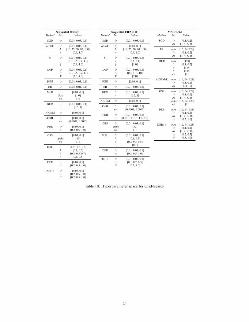
Sequential MNISTMethod Par Values

SGD lr [0.01, 0.03, 0.1]

oEWC lr [0.01, 0.03, 0.1]λ [10, 25, 30, 90, 100]γ [0.9, 1.0]

SI lr [0.01, 0.03, 0.1]c [0.3, 0.5, 0.7, 1.0]ξ [0.9, 1.0]

LwF lr [0.01, 0.03, 0.1]α [0.3, 0.5, 0.7, 1.0]T [2.0, 4.0]

PNN lr [0.01, 0.03, 0.1]

ER lr [0.03, 0.01, 0.1]

MER lr [0.03, 0.1]β, γ [1.0]nb [1]

GEM lr [0.01, 0.03, 0.1]γ [0.5, 1]

A-GEM lr [0.03, 0.1]

iCaRL lr [0.03, 0.1]wd [0.0001, 0.0005]

FDR lr [0.03, 0.1]α [0.2, 0.5, 1.0]

GSS lr [0.03, 0.1]gmbs [10]

nb [1]

HAL lr [0.03, 0.1, 0.2]λ [0.1, 0.5]β [0.2, 0.5, 0.7]γ [0.1, 0.5]

DER lr [0.03, 0.1]α [0.2, 0.5, 1.0]

DER++ lr [0.03, 0.1]α [0.2, 0.5, 1.0]β [0.2, 0.5, 1.0]

Sequential CIFAR-10Method Par Values

SGD lr [0.01, 0.03, 0.1]

oEWC lr [0.03, 0.1]λ [10, 25, 30, 90, 100]γ [0.9, 1.0]

SI lr [0.01, 0.03, 0.1]c [0.5, 0.1]ξ [1.0]

LwF lr [0.01, 0.03, 0.1]α [0.3, 1, 3, 10]T [2.0]

PNN lr [0.03, 0.1]

ER lr [0.01, 0.03, 0.1]

GEM lr [0.01, 0.03, 0.1]γ [0.5, 1]

A-GEM lr [0.03, 0.1]

iCaRL lr [0.01, 0.03, 0.1]wd [0.0001, 0.0005]

FDR lr [0.01, 0.03, 0.1]α [0.03, 0.1, 0.3, 1.0, 3.0]

GSS lr [0.01, 0.03, 0.1]gmbs [32]

nb [1]

HAL lr [0.01, 0.03, 0.1]λ [0.1, 0.5]β [0.2, 0.3, 0.5]γ [0.1]

DER lr [0.01, 0.03, 0.1]α [0.2, 0.5, 1.0]

DER++ lr [0.01, 0.03, 0.1]α [0.1, 0.2, 0.5]β [0.5, 1.0]

MNIST-360Method Par Values

SGD lr [0.1, 0.2]bs [1, 4, 8, 16]

ER mbs [16, 64, 128]lr [0.1, 0.2]bs [1, 4, 8, 16]

MER mbs [128]lr [0.1, 0.2]β [1.0]γ [1.0]nb [1]

A-GEM-R mbs [16, 64, 128]lr [0.1, 0.2]bs [1, 4, 16]

GSS mbs [16, 64, 128]lr [0.1, 0.2]bs [1, 4, 8, 16]

gmbs [16, 64, 128]nb [1]

DER mbs [16, 64, 128]lr [0.1, 0.2]bs [1, 4, 8, 16]α [0.5, 1.0]

DER++ mbs [16, 64, 128]lr [0.1, 0.2]bs [1, 4, 8, 16]α [0.2, 0.5]β [0.5, 1.0]

Table 10: Hyperparameter space for Grid-Search

24