dark energy and the accelerating universe - arxiv · dark energy and the accelerating universe...

arX

iv:0

803.

0982

v1 [

astr

o-ph

] 7

Mar

200

8

Dark Energy 1

Dark Energy and the Accelerating Universe

Joshua A. Frieman

Center for Particle Astrophysics, Fermi National Accelerator Laboratory, P. O.

Box 500, Batavia, IL 60510;

Kavli Institute for Cosmological Physics, The University of Chicago, 5640 S.

Ellis Ave., Chicago, IL 60637; email: [email protected]

Michael S. Turner

Kavli Institute for Cosmological Physics, The University of Chicago, 5640 S.

Ellis Ave., Chicago, IL 60637; email: [email protected]

Dragan Huterer

Department of Physics, University of Michigan, 450 Church St., Ann Arbor,

MI, 48109; email: [email protected]

Key Words cosmology, cosmological constant, supernovae, galaxy clusters, large-scale structure, weak gravitational lensing

Abstract

The discovery ten years ago that the expansion of the Universe is accelerating put in place thelast major building block of the present cosmological model, in which the Universe is composedof 4% baryons, 20% dark matter, and 76% dark energy. At the same time, it posed one of themost profound mysteries in all of science, with deep connections to both astrophysics and particlephysics. Cosmic acceleration could arise from the repulsive gravity of dark energy – for example,the quantum energy of the vacuum – or it may signal that General Relativity breaks down oncosmological scales and must be replaced. We review the present observational evidence forcosmic acceleration and what it has revealed about dark energy, discuss the various theoreticalideas that have been proposed to explain acceleration, and describe the key observational probesthat will shed light on this enigma in the coming years.

CONTENTS

INTRODUCTION . . . . . . . . . . . . . . . . . . . . . . . . . . . . . . . . . . . . 2

BASIC COSMOLOGY . . . . . . . . . . . . . . . . . . . . . . . . . . . . . . . . . 4Friedmann-Robertson-Walker cosmology . . . . . . . . . . . . . . . . . . . . . . . . . . 4Distances and the Hubble diagram . . . . . . . . . . . . . . . . . . . . . . . . . . . . . 7Growth of structure and ΛCDM . . . . . . . . . . . . . . . . . . . . . . . . . . . . . . . 8

FROM EINSTEIN TO ACCELERATED EXPANSION . . . . . . . . . . . . . . . 10Greatest blunder? . . . . . . . . . . . . . . . . . . . . . . . . . . . . . . . . . . . . . . . 10Steady state and after . . . . . . . . . . . . . . . . . . . . . . . . . . . . . . . . . . . . 11Enter inflation . . . . . . . . . . . . . . . . . . . . . . . . . . . . . . . . . . . . . . . . 11

http://arXiv.org/abs/0803.0982v1

Annu. Rev. Astron. Astrophys. 2008 46 XXX

Discovery . . . . . . . . . . . . . . . . . . . . . . . . . . . . . . . . . . . . . . . . . . . 12

CURRENT STATUS . . . . . . . . . . . . . . . . . . . . . . . . . . . . . . . . . . . 12Cosmic microwave background and large-scale structure . . . . . . . . . . . . . . . . . 13Recent supernova results . . . . . . . . . . . . . . . . . . . . . . . . . . . . . . . . . . . 15X-ray clusters . . . . . . . . . . . . . . . . . . . . . . . . . . . . . . . . . . . . . . . . . 15Age of the Universe . . . . . . . . . . . . . . . . . . . . . . . . . . . . . . . . . . . . . 16Cosmological parameters . . . . . . . . . . . . . . . . . . . . . . . . . . . . . . . . . . . 17

UNDERSTANDING COSMIC ACCELERATION . . . . . . . . . . . . . . . . . . 19Dark energy models . . . . . . . . . . . . . . . . . . . . . . . . . . . . . . . . . . . . . . 20Modified gravity . . . . . . . . . . . . . . . . . . . . . . . . . . . . . . . . . . . . . . . . 23Unmodified gravity . . . . . . . . . . . . . . . . . . . . . . . . . . . . . . . . . . . . . . 23Theory summary . . . . . . . . . . . . . . . . . . . . . . . . . . . . . . . . . . . . . . . 24

DESCRIBING DARK ENERGY . . . . . . . . . . . . . . . . . . . . . . . . . . . . 24Parametrizations . . . . . . . . . . . . . . . . . . . . . . . . . . . . . . . . . . . . . . . 25Direct reconstruction . . . . . . . . . . . . . . . . . . . . . . . . . . . . . . . . . . . . . 25Principal components . . . . . . . . . . . . . . . . . . . . . . . . . . . . . . . . . . . . . 26Kinematic description . . . . . . . . . . . . . . . . . . . . . . . . . . . . . . . . . . . . 27

PROBES OF COSMIC ACCELERATION . . . . . . . . . . . . . . . . . . . . . . 28Supernovae . . . . . . . . . . . . . . . . . . . . . . . . . . . . . . . . . . . . . . . . . . 28Clusters . . . . . . . . . . . . . . . . . . . . . . . . . . . . . . . . . . . . . . . . . . . . 30Baryon acoustic oscillations . . . . . . . . . . . . . . . . . . . . . . . . . . . . . . . . . 32Weak gravitational lensing . . . . . . . . . . . . . . . . . . . . . . . . . . . . . . . . . . 33Other probes . . . . . . . . . . . . . . . . . . . . . . . . . . . . . . . . . . . . . . . . . 35Role of the CMB . . . . . . . . . . . . . . . . . . . . . . . . . . . . . . . . . . . . . . . 36Probing new gravitational physics . . . . . . . . . . . . . . . . . . . . . . . . . . . . . . 36Summary and comparison . . . . . . . . . . . . . . . . . . . . . . . . . . . . . . . . . . 37

DARK ENERGY PROJECTS . . . . . . . . . . . . . . . . . . . . . . . . . . . . . 38Ground-based surveys . . . . . . . . . . . . . . . . . . . . . . . . . . . . . . . . . . . . 39Space-based surveys . . . . . . . . . . . . . . . . . . . . . . . . . . . . . . . . . . . . . . 40

DARK ENERGY & COSMIC DESTINY . . . . . . . . . . . . . . . . . . . . . . . 41

CONCLUDING REMARKS . . . . . . . . . . . . . . . . . . . . . . . . . . . . . . 43Take-home facts . . . . . . . . . . . . . . . . . . . . . . . . . . . . . . . . . . . . . . . 44Open issues and challenges . . . . . . . . . . . . . . . . . . . . . . . . . . . . . . . . . 45

APPENDIX . . . . . . . . . . . . . . . . . . . . . . . . . . . . . . . . . . . . . . . . 47Figure(s) of merit . . . . . . . . . . . . . . . . . . . . . . . . . . . . . . . . . . . . . . 47Fisher information matrix . . . . . . . . . . . . . . . . . . . . . . . . . . . . . . . . . . 47

1 INTRODUCTION

In 1998, two teams studying distant Type Ia supernovae presented independentevidence that the expansion of the Universe is speeding up (Perlmutter et al.1999, Riess et al. 1998). Since Hubble, cosmologists had been trying to measurethe slowing of the expansion due to gravity; so expected was slow-down that theparameter used to quantify the second derivative of the expansion, q0, was calledthe deceleration parameter (Sandage 1962). The discovery of cosmic accelerationis arguably one of the most important developments in modern cosmology.

The ready acceptance of the supernova results was not a foregone conclusion.

2

Dark Energy 3

The cosmological constant, the simplest explanation of accelerated expansion,had a checkered history, having been invoked and subsequently withdrawn sev-eral times before. This time, however, subsequent observations, including moredetailed studies of supernovae and independent evidence from clusters of galaxies,large-scale structure, and the cosmic microwave background (CMB), confirmedand firmly established this remarkable finding.

The physical origin of cosmic acceleration remains a deep mystery. Accordingto General Relativity (GR), if the Universe is filled with ordinary matter orradiation, the two known constituents of the Universe, gravity should lead toa slowing of the expansion. Since the expansion is speeding up, we are facedwith two possibilities, either of which would have profound implications for ourunderstanding of the cosmos and of the laws of physics. The first is that 75%of the energy density of the Universe exists in a new form with large negativepressure, called dark energy. The other possibility is that General Relativitybreaks down on cosmological scales and must be replaced with a more completetheory of gravity.

Through a tangled history, dark energy is tied to Einstein’s cosmological con-stant, Λ. Einstein introduced Λ into the field equations of General Relativityin order to produce a static, finite cosmological model (Einstein 1917). Withthe discovery of the expansion of the Universe, the rationale for the cosmologicalconstant evaporated. Fifty years later, Zel’dovich (1968) realized that Λ, math-ematically equivalent to the stress-energy of empty space—the vacuum—cannotsimply be dismissed. In quantum field theory, the vacuum state is filled with vir-tual particles, and their effects have been measured in the shifts of atomic linesand in particle masses. However, estimates for the energy density associatedwith the quantum vacuum are at least 60 orders of magnitude too large and insome cases infinite, a major embarrassment known as the cosmological constantproblem (Weinberg 1989).

Despite the troubled history of Λ, the observational evidence for cosmic accel-eration was quickly embraced by cosmologists, because it provided the missingelement needed to complete the current cosmological model. In this model, theUniverse is spatially flat and accelerating; composed of baryons, dark matter, anddark energy; underwent a hot, dense, early phase of expansion that produced thelight elements via big bang nucleosynthesis and the CMB radiation; and experi-enced a much earlier epoch of accelerated expansion, known as inflation, whichproduced density perturbations from quantum fluctuations, leaving an imprinton the CMB anisotropy and leading by gravitational instability to the formationof large-scale structure.

The current cosmological model also raises deep issues, from the origin of theexpansion itself and the nature of dark matter to the genesis of baryons andthe cause of accelerated expansion. Of all these, the mystery of cosmic accelera-tion may be the richest, with broad connections to other important questions incosmology and in particle physics. For example, the destiny of the Universe istied to understanding dark energy; primordial inflation also involves acceleratedexpansion and its cause may be related; dark matter and dark energy could belinked; cosmic acceleration could provide a key to finding a successor to Einstein’stheory of gravity; the smallness of the energy density of the quantum vacuummight reveal something about supersymmetry or even superstring theory; andthe cause of cosmic acceleration could give rise to new long-range forces or berelated to the smallness of neutrino masses.

4 Frieman, Turner & Huterer

This review is organized into three parts. The first part is devoted to Context:in §2 we briefly review the Friedmann-Robertson-Walker (FRW) cosmology, theframework for understanding how observational probes of dark energy work. §3provides the historical context, from Einstein’s introduction of the cosmologicalconstant to the supernova discovery. Part Two covers Current Status: in §4,we review the web of observational evidence that firmly establishes acceleratedexpansion. §5 summarizes current theoretical approaches to accelerated expan-sion and dark energy, including discussion of the cosmological constant problem,models of dark energy, and modified gravity, while §6 focuses on different phe-nomenological descriptions of dark energy and their relative merits. Part Threeaddresses The Future: §7 discusses the observational techniques that will be usedto probe dark energy, primarily supernovae, weak lensing, large-scale structure,and clusters. In §8, we discuss specific projects aimed at constraining dark energyplanned for the next fifteen years which have the potential to provide insightsinto the origin of cosmic acceleration. The connection between the future of theUniverse and dark energy is the topic of §9. We summarize in §10, framing thetwo big questions about cosmic acceleration where progress should be made inthe next fifteen years – Is dark energy something other than vacuum energy?Does General Relativity self-consistently describe cosmic acceleration? – anddiscussing what we believe are the most important open issues.

Our goal is to broadly review cosmic acceleration for the astronomy commu-nity. A number of useful reviews target different aspects of the subject, includ-ing: theory (Copeland, Sami & Tsujikawa 2006; Padmanabhan 2003); cosmology(Peebles & Ratra 2003); the physics of cosmic acceleration (Uzan 2007); probesof dark energy (Huterer & Turner 2001); dark energy reconstruction (Sahni &Starobinsky 2006); dynamics of dark energy models (Linder 2007); the cosmolog-ical constant (Carroll 2001; Carroll, Press & Turner 1992), and the cosmologicalconstant problem (Weinberg 1989).

2 BASIC COSMOLOGY

In this section, we provide a brief review of the elements of the FRW cosmolog-ical model. This model provides the context for interpreting the observationalevidence for cosmic acceleration as well as the framework for understanding howcosmological probes in the future will help uncover the cause of acceleration bydetermining the history of the cosmic expansion with greater precision. For fur-ther details on basic cosmology, see, e.g., the textbooks of Dodelson (2003), Kolb& Turner (1990), Peacock (1999), and Peebles (1993). Note that we follow thestandard practice of using units in which the speed of light c = 1.

2.1 Friedmann-Robertson-Walker cosmology

From the large-scale distribution of galaxies and the near-uniformity of the CMBtemperature, we have good evidence that the Universe is nearly homogeneousand isotropic. Under this assumption, the spacetime metric can be written in theFRW form,

ds2 = dt2 − a2(t)[

dr2/(1 − kr2) + r2dθ2 + r2 sin2 θdφ2]

, (1)

where r, θ, φ are comoving spatial coordinates, t is time, and the expansion isdescribed by the cosmic scale factor, a(t) (by convention, a = 1 today). The

Dark Energy 5

quantity k is the curvature of 3-dimensional space: k = 0 corresponds to aspatially flat, Euclidean Universe, k > 0 to positive curvature (3-sphere), andk < 0 to negative curvature (saddle).

The wavelengths λ of photons moving through the Universe scale with a(t),and the redshift of light emitted from a distant source at time tem, 1 + z =λobs/λem = 1/a(tem), directly reveals the relative size of the Universe at thattime. This means that time intervals are related to redshift intervals by dt =−dz/H(z)(1 + z), where H ≡ a/a is the Hubble parameter, and an overdotdenotes a time derivative. The present value of the Hubble parameter is conven-tionally expressed as H0 = 100 h km/sec/Mpc, where h ≈ 0.7 is the dimensionlessHubble parameter. Here and below, a subscript “0” on a parameter denotes itsvalue at the present epoch.

The key equations of cosmology are the Friedmann equations, the field equa-tions of GR applied to the FRW metric,

H2 =

(

a

a

)2

=8πGρ

3− k

a2+

Λ

3(2)

a

a= −4πG

3(ρ + 3p) +

Λ

3(3)

where ρ is the total energy density of the Universe (sum of matter, radiation,dark energy), and p is the total pressure (sum of pressures of each component).For historical reasons we display the cosmological constant Λ here; hereafter, weshall always represent it as vacuum energy and subsume it into the density andpressure terms; the correspondence is: Λ = 8πGρVAC = −8πGpVAC.

For each component, the conservation of energy is expressed by d(a3ρi) =−pida3, the expanding Universe analogue of the first law of thermodynamics,dE = −pdV . Thus, the evolution of energy density is controlled by the ratio ofthe pressure to the energy density, the equation-of-state parameter, wi ≡ pi/ρi.

1

For the general case, this ratio varies with time, and the evolution of the energydensity in a given component is given by

ρi ∝ exp

[

3

∫ z

0[1 + wi(z

′)]d ln(1 + z′)

]

. (4)

In the case of constant wi,

wi ≡pi

ρi= constant , ρi ∝ (1 + z)3(1+wi) . (5)

For non-relativistic matter, which includes both dark matter and baryons, wM = 0to very good approximation, and ρM ∝ (1 + z)3; for radiation, i.e., relativisticparticles, wR = 1/3, and ρR ∝ (1 + z)4. For vacuum energy, as noted abovepVAC = −ρVAC = −Λ/8πG = constant, i.e., wVAC = −1. For other models of

1A perfect fluid is fully characterized by its isotropic pressure p and energy density ρ, wherep is a function of density and other state variables (e.g., temperature). The equation-of-stateparameter w = p/ρ determines the evolution of the energy density ρ; e.g., ρ ∝ V 1+w forconstant w, where V is the volume occupied by the fluid. Vacuum energy or a homogeneousscalar field are spatially uniform and they too can be fully characterized by w. The evolutionof an inhomogeneous, imperfect fluid is in general complicated and not fully described by w.Nonetheless, in the FRW cosmology, spatial homogeneity and isotropy require the stress-energyto take the perfect fluid form; thus, w determines the evolution of the energy density.


dark energy, w can differ from −1 and vary in time. [Hereafter, w without asubscript refers to dark energy.]

The present energy density of a flat Universe (k = 0), ρcrit ≡ 3H20/8πG =

1.88× 10−29h2gm cm−3 = 8.10× 10−47h2 GeV4, is known as the critical density;it provides a convenient means of normalizing cosmic energy densities, whereΩi = ρi(t0)/ρcrit. For a positively curved Universe, Ω0 ≡ ρ(t0)/ρcrit > 1 and fora negatively curved Universe Ω0 < 1. The present value of the curvature radius,Rcurv ≡ a/

√

|k|, is related to Ω0 and H0 by Rcurv = H−10 /

√

|Ω0 − 1|, and the

characteristic scale H−10 ≈ 3000h−1 Mpc is known as the Hubble radius. Because

of the evidence from the CMB that the Universe is nearly spatially flat (see Fig.8), we shall assume k = 0 except where otherwise noted.

-101234Log [1+z]

-48

-44

-40

-36

Log

[en

ergy

den

sity

(G

eV4 )]

radiation matter

dark energy

Figure 1: Evolution of radiation, matter, and dark energy densities with redshift.For dark energy, the band represents w = −1 ± 0.2.

Fig. 1 shows the evolution of the radiation, matter, and dark energy densitieswith redshift. The Universe has gone through three distinct eras: radiation-dominated, z & 3000; matter-dominated, 3000 & z & 0.5; and dark-energydominated, z ∼< 0.5. The evolution of the scale factor is controlled by the

dominant energy form: a(t) ∝ t2/3(1+w) (for constant w). During the radiation-dominated era, a(t) ∝ t1/2; during the matter-dominated era, a(t) ∝ t2/3; andfor the dark energy-dominated era, assuming w = −1, asymptotically a(t) ∝exp(Ht). For a flat Universe with matter and vacuum energy, the general solu-tion, which approaches the latter two above at early and late times, is a(t) =(ΩM/ΩVAC)1/3(sinh[3

√ΩVACH0t/2])

2/3.The deceleration parameter, q(z), is defined as

q(z) ≡ − a

aH2=

1

2

∑

i

Ωi(z) [1 + 3wi(z)] (6)

where Ωi(z) ≡ ρi(z)/ρcrit(z) is the fraction of critical density in component iat redshift z. During the matter- and radiation-dominated eras, wi > 0 and

Dark Energy 7

gravity slows the expansion, so that q > 0 and a < 0. Because of the (ρ +3p) term in the second Friedmann equation (Newtonian cosmology would onlyhave ρ), the gravity of a component that satisfies p < −ρ/3, i.e., w < −1/3, isrepulsive and can cause the expansion to accelerate (a > 0): we take this to bethe defining property of dark energy. The successful predictions of the radiation-dominated era of cosmology, e.g., big bang nucleosynthesis and the formation ofCMB anisotropies, provide evidence for the (ρ+3p) term, since during this epocha is about twice as large as it would be in Newtonian cosmology.

2.2 Distances and the Hubble diagram

For an object of intrinsic luminosity L, the measured energy flux F defines theluminosity distance dL to the object, i.e., the distance inferred from the inversesquare law. The luminosity distance is related to the cosmological model through

dL(z) ≡√

L

4πF= (1 + z)r(z) , (7)

where r(z) is the comoving distance to an object at redshift z,

r(z) =

∫ z

0

dz′

H(z′)=

∫ 1

1/(1+z)

da

a2H(a)(k = 0) , (8)

r(z) = |k|−1/2χ

[

|k|1/2

∫ z

0dz′/H(z′)

]

(k 6= 0) , (9)

and where χ(x) = sin(x) for k > 0 and sinh(x) for k < 0. Specializing to the flatmodel and constant w,

r(z) =1

H0

∫ z

0

dz′√

ΩM(1 + z′)3 + (1 − ΩM)(1 + z′)3(1+w) + ΩR(1 + z′)4(10)

where ΩM is the present fraction of critical density in non-relativistic matter, andΩR ≃ 0.8 × 10−4 represents the small contribution to the present energy densityfrom photons and relativistic neutrinos. In this model, the dependence of cosmicdistances upon dark energy is controlled by the parameters ΩM and w and isshown in the left panel of Fig. 2.

The luminosity distance is related to the distance modulus µ by

µ(z) ≡ m − M = 5 log10 (dL/10 pc) = 5 log10 [(1 + z)r(z)/pc] − 5 , (11)

where m is the apparent magnitude of the object (proportional to the log ofthe flux) and M is the the absolute magnitude (proportional to the log of theintrinsic luminosity). “Standard candles,” objects of fixed absolute magnitudeM , and measurements of the logarithmic energy flux m constrain the cosmolog-ical model and thereby the expansion history through this magnitude-redshiftrelation, known as the Hubble diagram.

Expanding the scale factor around its value today, a(t) = 1 + H0(t − t0) −q0H

20 (t−t0)

2/2+· · · , the distance-redshift relation can be written in its historicalform

H0dL = z +1

2(1 − q0)z

2 + · · · (12)

The expansion rate and deceleration rate today appear in the first two terms inthe Taylor expansion of the relation. This expansion, only valid for z ≪ 1, is of


0.0 0.5 1.0 1.5 2.0redshift z

0.0

0.5

1.0

1.5H

0 r(z

)

ΩM

=0.2, w=-1.0

ΩM

=0.3, w=-1.0

ΩM

=0.2, w=-1.5

ΩM

=0.2, w=-0.5

0.0 0.5 1.0 1.5 2.0redshift z

0.0

0.5

1.0

(d2 V

/dΩ

dz)

x (H

03 / z2 ) Ω

M=0.2, w=-1.0

ΩM

=0.3, w=-1.0

ΩM

=0.2, w=-1.5

ΩM

=0.2, w=-0.5

Figure 2: For a flat Universe, the effect of dark energy upon cosmic distance (left)and volume element (right) is controlled by ΩM and w.

historical significance and utility; it is not useful today since objects as distantas redshift z ∼ 2 are being used to probe the expansion history. However, itdoes illustrate the general principle: the first term on the r.h.s. represents thelinear Hubble expansion, and the deviation from a linear relation reveals thedeceleration (or acceleration).

The angular-diameter distance dA, the distance inferred from the angular sizeδθ of a distant object of fixed diameter D, is defined by dA ≡ D/δθ = r(z)/(1 +z) = dL/(1 + z)2. The use of “standard rulers” (objects of fixed intrinsic size)provides another means of probing the expansion history, again through r(z).

The cosmological time, or time back to the Big Bang, is given by

t(z) =

∫ t(z)

0dt′ =

∫ ∞

z

dz′

(1 + z′)H(z′). (13)

While the present age in principle depends upon the expansion rate at very earlytimes, the rapid rise of H(z) with z — a factor of 30,000 between today and theepoch of last scattering, when photons and baryons decoupled, at zLS ≃ 1100,t(zLS) ≃ 380, 000 years — makes this point moot.

Finally, the comoving volume element per unit solid angle dΩ is given by

d2V

dzdΩ= r2 dr

dz

1√1 − kr2

=r2(z)

H(z). (14)

For a set of objects of known comoving density n(z), the comoving volume elementcan be used to infer r2(z)/H(z) from the number counts per unit redshift and solidangle, d2N/dzdΩ = n(z)d2V/dzdΩ. The dependence of the comoving volumeelement upon ΩM and w is shown in the right panel of Fig. 2.

2.3 Growth of structure and ΛCDM

A striking success of the consensus cosmology is its ability to account for theobserved structure in the Universe, provided that the dark matter is composed of

Dark Energy 9

0.11.010.0z

0.1

1

δ(z)

/δ(to

day)

w=−1

w=−1/3

Figure 3: Growth of linear density perturbations in a flat universe with darkenergy. Note that the growth of perturbations ceases when dark energy beginsto dominate, 1 + z = (ΩM/ΩDE)1/3w.

slowly moving particles, known as cold dark matter (CDM), and that the initialpower spectrum of density perturbations is nearly scale-invariant, P (k) ∼ knS

with spectral index nS ≃ 1, as predicted by inflation (Springel, Frenk & White2006). Dark energy affects the development of structure by its influence on theexpansion rate of the Universe when density perturbations are growing. Thisfact and the quantity and quality of large-scale structure data make structureformation a sensitive probe of dark energy.

In GR the growth of small-amplitude, matter-density perturbations on lengthscales much smaller than the Hubble radius is governed by

δk + 2Hδk − 4πGρMδk = 0 , (15)

where the perturbations δ(x, t) ≡ δρM(x, t)/ρM(t) have been decomposed intotheir Fourier modes of wavenumber k, and matter is assumed to be pressureless(always true for the CDM portion and valid for the baryons on mass scales largerthan 105 M⊙ after photon-baryon decoupling). Dark energy affects the growththrough the “Hubble damping” term, 2Hδk.

The solution to Eq. (15) is simple to describe during the three epochs of ex-pansion discussed earlier: δk(t) grows as a(t) during the matter-dominated epochand is approximately constant during the radiation-dominated and dark energy-dominated epochs. The key feature here is the fact that once accelerated expan-sion begins, the growth of linear perturbations effectively ends, since the Hubbledamping time becomes shorter than the timescale for perturbation growth.

The impact of the dark energy equation-of-state parameter w on the growth ofstructure is more subtle and is illustrated in Fig. 3. For larger w and fixed darkenergy density ΩDE, dark energy comes to dominate earlier, causing the growth oflinear perturbations to end earlier; this means the growth factor since decouplingis smaller and that to achieve the same amplitude by today, the perturbationmust begin with larger amplitude and is larger at all redshifts until today. Thesame is true for larger ΩDE and fixed w. Finally, if dark energy is dynamical (notvacuum energy), then in principle it can be inhomogeneous, an effect ignored


above. In practice, it is expected to be nearly uniform over scales smaller thanthe present Hubble radius, in sharp contrast to dark matter, which can clump onsmall scales.

3 FROM EINSTEIN TO ACCELERATED EXPANSION

Although the discovery of cosmic acceleration is often portrayed as a major sur-prise and a radical contravention of the conventional wisdom, it was anticipatedby a number of developments in cosmology in the preceding decade. Moreover,this is not the first time that the cosmological constant has been proposed. In-deed, the cosmological constant was explored from the very beginnings of GeneralRelativity and has been periodically invoked and subsequently cast aside severaltimes since. Here we recount some of this complex 90-year history.

3.1 Greatest blunder?

Einstein introduced the cosmological constant in his field equations in order toobtain a static and finite cosmological solution “as required by the fact of thesmall velocities of the stars” and to be consistent with Mach’s principle (Einstein1917). In Einstein’s solution, space is positively curved, Rcurv = 1/

√4πGρM, and

the “repulsive gravity” of Λ is balanced against the attractive gravity of matter,ρΛ = ρM/2. In the 1920’s, Friedmann and Lemaıtre independently showed thatcosmological solutions with matter and Λ generally involved expansion or con-traction, and Lemaıtre as well as Eddington showed that Einstein’s static solutionwas unstable to expansion or contraction. In 1917, de Sitter explored a solutionin which ρM is negligible compared to ρΛ (de Sitter 1917). There was some earlyconfusion about the interpretation of this model, but in the early 1920’s, Weyl,Eddington, and others showed that the apparent recession velocity (the redshift)at small separation would be proportional to the distance, v =

√

Λ/3 d.With Hubble’s discovery of the expansion of the Universe in 1929, Einstein’s

primary justification for introducing the cosmological constant was lost, and headvocated abandoning it. Gamow later wrote that Einstein called this “his great-est blunder,” since he could have predicted the expanding Universe. Yet the de-scription above makes it clear that the history was more complicated, and onecould argue that in fact Friedmann and Lemaıtre (or de Sitter) had “predicted”the expanding Universe, Λ or no. Indeed, Hubble noted that his linear relationbetween redshift and distance was consistent with the prediction of the de Sittermodel (Hubble 1929). Moreover, Eddington recognized that Hubble’s value forthe expansion rate, H0 ≃ 570 km/s/Mpc, implied a time back to the big bang ofless than 2 Gyr, uncomfortably short compared to some age estimates of Earthand the galaxy. By adjusting the cosmological constant to be slightly largerthan the Einstein value, ρΛ = (1 + ǫ)ρM/2, a nearly static beginning of arbi-trary duration could be obtained, a solution known as the Eddington-Lemaıtremodel. While Eddington remained focused on Λ, trying to find a place for itin his “unified” and “fundamental” theories, Λ was no longer the focus of mostcosmologists.

Dark Energy 11

3.2 Steady state and after

Motivated by the aesthetic beauty of an unchanging Universe, Bondi & Gold(1948) and Hoyle (1948) put forth the steady-state cosmology, a revival of the deSitter model with a new twist. In the steady-state model, the dilution of matterdue to expansion is counteracted by postulating the continuous creation of matter(about 1 hydrogen atom/m3/Gyr). However, the model’s firm prediction of anunevolving Universe made it easily falsifiable, and the redshift distribution ofradio galaxies, the absence of quasars nearby, and the discovery of the cosmicmicrowave background radiation did so in the early 1960s.

Λ was briefly resurrected again in the late 1960s by Petrosian, Salpeter &Szekeres (1967), who used the Eddington-Lemaıtre model to explain the prepon-derance of quasars at redshifts around z ∼ 2. As it turns out, this is a realobservational effect, but it can be attributed to evolution: quasar activity peaksaround this redshift. In 1975, evidence for a cosmological constant from the Hub-ble diagram of brightest-cluster elliptical galaxies was presented (Gunn & Tinsley1975), though it was realized (Tinsley & Gunn 1976) that uncertainties in galaxyluminosity evolution make their use as standard candles problematic.

While cosmologists periodically hauled the cosmological constant out of thecloset as needed and then stuffed it back in, in the 1960s physicists began tounderstand that Λ cannot be treated in such cavalier fashion. With the riseof the standard big-bang cosmology came the awareness that the cosmologicalconstant could be a big problem (Zel’dovich 1968). It was realized that theenergy density of the quantum vacuum should result in a cosmological constantof enormous size (see §5.1.1). However, because of the success of the hot big-bangmodel, the lack of compelling ideas to solve the cosmological constant problem,and the dynamical unimportance of Λ at the early epochs when the hot big-bangmodel was best tested by big-bang nucleosynthesis and the CMB, the problemwas largely ignored in cosmological discourse.

3.3 Enter inflation

In the early 1980s the inflationary universe scenario (Guth 1981), with its pre-dictions of a spatially flat Universe (Ω = 1) and almost-scale-invariant densityperturbations, changed the cosmological landscape and helped set the stage forthe discovery of cosmic acceleration. When inflation was first introduced, theevidence for dark matter was still accruing, and estimates of the total matterdensity, then about ΩM ∼ 0.1, were sufficiently uncertain that an Einstein-deSitter model (i.e., ΩM = 1) was not ruled out. The evidence for a low value ofΩM was, however, sufficiently worrisome that the need for a smooth component,such as vacuum energy, to make up the difference for a flat Universe was sug-gested (Peebles 1984; Turner, Steigman & Krauss 1984). Later, the model forlarge-scale structure formation with a cosmological constant and cold dark mat-ter (ΛCDM) and the spectrum of density perturbations predicted by inflationwas found to provide a better fit (than ΩM = 1) to the growing observationsof large-scale structure (Efstathiou, Sutherland & Maddox 1990; Turner 1991).The 1992 COBE discovery of CMB anisotropy provided the normalization of thespectrum of density perturbations and drove a spike into the heart of the ΩM = 1CDM model.

Another important thread involved age consistency. While estimates of the


Hubble parameter had ranged between 50 and 100 km/s/Mpc since the 1970s,by the mid-1990s they were settling out in the middle of that range. Estimatesof old globular cluster ages had similar swings, but had settled at t0 ≃ 13 − 15Gyr. The resulting expansion age, H0t0 = (H0/70 km/s/Mpc)(t0/14 Gyr) wasuncomfortably high compared to that for the Einstein-de Sitter model, for whichH0t0 = 2/3. The cosmological constant offered a ready solution, as the age of aflat Universe with Λ rises with ΩΛ,

H0t0 =1

3Ω1/2Λ

ln

[

1 + ΩΛ1/2

1 − ΩΛ1/2

]

=2

3

[

1 + ΩΛ2/3 + ΩΛ

4/5 + · · ·]

, (16)

reaching H0t0 ≃ 1 for ΩΛ = 0.75.By 1995 the cosmological constant was back out of the cosmologists’ closet in

full glory (Frieman et al. 1995, Krauss & Turner 1995, Ostriker & Steinhardt1995): it solved the age problem, was consistent with growing evidence that ΩM

was around 0.3, and fit the growing body of observations of large-scale structure.Its only serious competitors were “open inflation,” which had a small group ofadherents, and hot + cold dark matter, with a low value for the Hubble parameter(∼ 50 km/s/Mpc) and neutrinos accounting for 10% to 15% of the dark matter(see, e.g., contributions in Turok 1997). During this period, there were tworesults that conflicted with ΛCDM: analysis of the statistics of lensed quasars(Kochanek 1996) and of the first 7 high-redshift supernovae of the SupernovaCosmology Project (Perlmutter et al. 1997) respectively indicated that ΩΛ < 0.66and ΩΛ < 0.51 at 95% confidence, for a flat Universe. The discovery of acceleratedexpansion in 1998 saved inflation by providing evidence for large ΩΛ and was thuswelcome news for cosmology.

3.4 Discovery

Two breakthroughs enabled the discovery of cosmic acceleration. The first wasthe demonstration that type Ia supernovae (SNe Ia) are standardizable candles(Phillips 1993). The second was the deployment of large mosaic CCD camerason 4-meter class telescopes, enabling the systematic search of large areas of sky,containing thousands of galaxies, for these rare events. By comparing deep, wideimages taken weeks apart, the discovery of SNe at redshifts z ∼ 0.5 could be“scheduled” on a statistical basis.

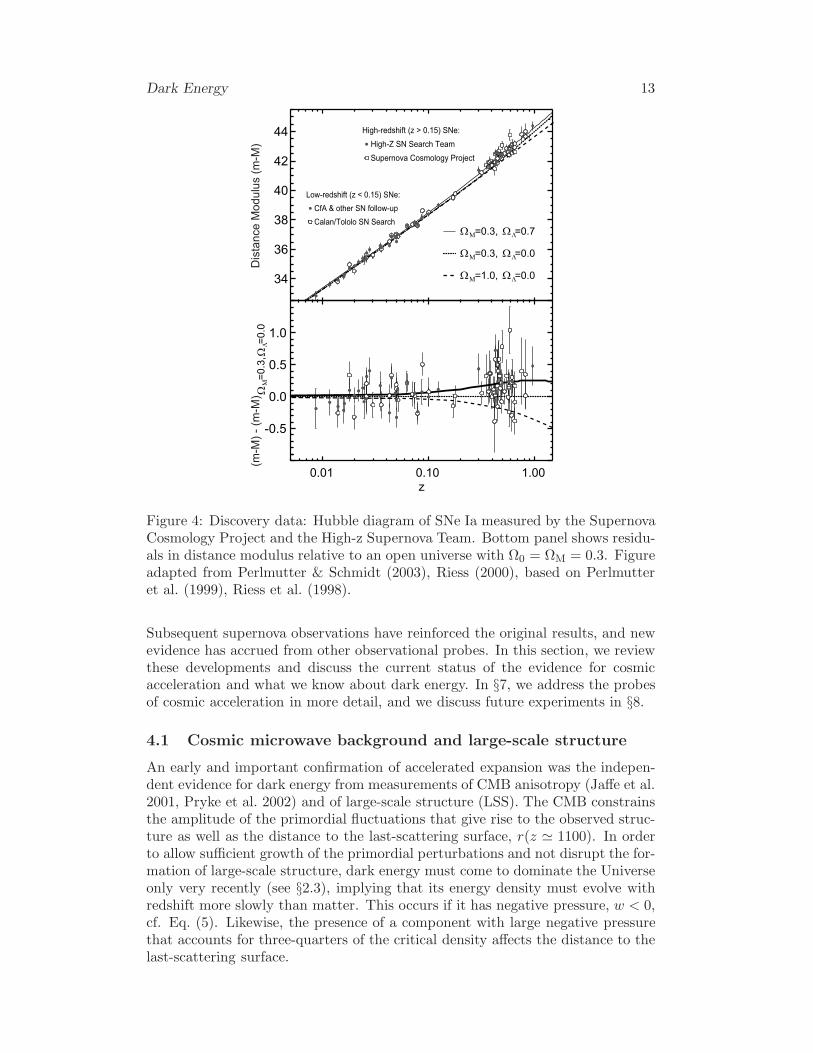
Two teams, the Supernova Cosmology Project and the High-z SN Search, work-ing independently in the mid- to late-1990s took advantage of these breakthroughsto measure the SN Hubble diagram to much larger distances than was previouslypossible. Both teams found that distant SNe are ∼ 0.25 mag dimmer than theywould be in a decelerating Universe, indicating that the expansion has beenspeeding up for the past 5 Gyr (Perlmutter et al. 1999, Riess et al. 1998); seeFig. 4. When analyzed assuming a Universe with matter and cosmological con-stant, their results provided evidence for ΩΛ > 0 at greater than 99% confidence(see Fig. 8 for the current constraints).

4 CURRENT STATUS

Since the supernova discoveries were announced in 1998, the evidence for anaccelerating Universe has become substantially stronger and more broadly based.

Dark Energy 13

Supernova Cosmology Project

34

36

38

40

42

44

WM=0.3, WL=0.7

WM=0.3, WL=0.0

WM=1.0, WL=0.0

High-Z SN Search Team

-0.5

0.0

0.5

1.0

WM=0

.3, W

L=0.

0

0.01 0.10 1.00z

High-redshift (z > 0.15) SNe:

Calan/Tololo SN SearchCfA & other SN follow-up

Low-redshift (z < 0.15) SNe:

Dist

ance

Mod

ulus

(m-M

) (m

-M) -

(m-M

)

Figure 4: Discovery data: Hubble diagram of SNe Ia measured by the SupernovaCosmology Project and the High-z Supernova Team. Bottom panel shows residu-als in distance modulus relative to an open universe with Ω0 = ΩM = 0.3. Figureadapted from Perlmutter & Schmidt (2003), Riess (2000), based on Perlmutteret al. (1999), Riess et al. (1998).

Subsequent supernova observations have reinforced the original results, and newevidence has accrued from other observational probes. In this section, we reviewthese developments and discuss the current status of the evidence for cosmicacceleration and what we know about dark energy. In §7, we address the probesof cosmic acceleration in more detail, and we discuss future experiments in §8.

4.1 Cosmic microwave background and large-scale structure

An early and important confirmation of accelerated expansion was the indepen-dent evidence for dark energy from measurements of CMB anisotropy (Jaffe et al.2001, Pryke et al. 2002) and of large-scale structure (LSS). The CMB constrainsthe amplitude of the primordial fluctuations that give rise to the observed struc-ture as well as the distance to the last-scattering surface, r(z ≃ 1100). In orderto allow sufficient growth of the primordial perturbations and not disrupt the for-mation of large-scale structure, dark energy must come to dominate the Universeonly very recently (see §2.3), implying that its energy density must evolve withredshift more slowly than matter. This occurs if it has negative pressure, w < 0,cf. Eq. (5). Likewise, the presence of a component with large negative pressurethat accounts for three-quarters of the critical density affects the distance to thelast-scattering surface.


Figure 5: Left panel: Angular power spectrum measurements of the CMB tem-perature fluctuations from WMAP, Boomerang, and ACBAR. Red curve showsthe best-fit ΛCDM model. From Reichardt et al. (2008). Right panel: Detectionof the baryon acoustic peak in the clustering of luminous red galaxies in the SDSS(Eisenstein et al. 2005). Shown is the two-point galaxy correlation function inredshift space; inset shows an expanded view with a linear vertical axis. Curvescorrespond to ΛCDM predictions for ΩMh2 = 0.12 (green), 0.13 (red), and 0.14(blue). Magenta curve shows a ΛCDM model without BAO.

4.1.1 CMB Anisotropies of the cosmic microwave background provide arecord of the Universe at a simpler time, before structure had developed andwhen photons were decoupling from baryons, about 380,000 years after the BigBang (Hu & Dodelson 2002). The angular power spectrum of CMB temperatureanisotropies, measured most recently by WMAP (Spergel et al. 2007) and byground-based experiments that probe to smaller angular scales, is dominatedby acoustic peaks that arise from gravity-driven sound waves in the photon-baryon fluid (see Fig. 5a). The positions and amplitudes of the acoustic peaksencode a wealth of cosmological information. They indicate that the Universeis nearly spatially flat to within a few percent. In combination with LSS orwith independent H0 measurement, the CMB measurements indicate that mattercontributes only about a quarter of the critical density. A component of missingenergy that is smoothly distributed is needed to square these observations – andis fully consistent with the dark energy needed to explain accelerated expansion.

4.1.2 Large-scale Structure Baryon acoustic oscillations (BAO), soprominent in the CMB anisotropy, leave a subtler characteristic signature in theclustering of galaxies, a bump in the two-point correlation function at a scale∼ 100 Mpc that can be measured today and in the future can provide a powerfulprobe of dark energy (see §7.3). Measurement of the BAO signature in thecorrelation function of SDSS luminous red galaxies (see Fig. 5b) constrains thedistance to redshift z = 0.35 to a precision of 5% (Eisenstein et al. 2005). Thismeasurement serves as a significant complement to other probes, as shown inFig. 8.

The presence of dark energy affects the large-angle anisotropy of the CMB(the low-ℓ multipoles) through the integrated Sachs-Wolfe (ISW) effect. The

Dark Energy 15

ISW arises due to the differential redshifts of photons as they pass through time-changing gravitational potential wells, and it leads to a small correlation betweenthe low-redshift matter distribution and the CMB anisotropy. This effect hasbeen observed in the cross-correlation of the CMB with galaxy and radio sourcecatalogs (Afshordi, Loh & Strauss 2004; Boughn & Crittenden 2004; Fosalba &Gaztanaga 2004; Scranton et al. 2003). This signal indicates that the Universe isnot described by the Einstein-de Sitter model (ΩM = 1), a reassuring cross-check.

Weak gravitational lensing (Munshi et al. 2006, Schneider 2006), the small,correlated distortions of galaxy shapes due to gravitational lensing by interveninglarge-scale structure, is a powerful technique for mapping dark matter and itsclustering. Detection of this cosmic shear signal was first announced by fourgroups in 2000 (Bacon, Refregier & Ellis 2000; Kaiser, Wilson & Luppino 2000;Van Waerbeke et al. 2000; Wittman et al. 2000). Recent lensing surveys coveringareas of order 100 square degrees have shed light on dark energy by pinning downthe combination σ8(ΩM/0.25)0.6 ≈ 0.85 ± 0.07, where σ8 is the rms amplitudeof mass fluctuations on the 8 h−1 Mpc scale (Hoekstra et al. 2006, Jarvis et al.2006, Massey et al. 2007). Since other measurements peg σ8 at ≃ 0.8, this impliesthat ΩM ≃ 0.25, consistent with a flat Universe dominated by dark energy. Inthe future, weak lensing has the potential to be the most powerful probe of darkenergy (Hu 2002, Huterer 2002), and this is discussed in §7 and §8.

4.2 Recent supernova results

A number of concerns were raised about the robustness of the first SN evidencefor acceleration, e.g., it was suggested that distant SNe could appear fainter dueto extinction by hypothetical grey dust rather than acceleration (Aguirre 1999;Drell, Loredo & Wasserman 2000). Over the intervening decade, the supernovaevidence for acceleration has been strengthened by results from a series of SNsurveys. Observations with the Hubble Space Telescope (HST) have providedhigh-quality light curves (Knop et al. 2003) and have extended SN measurementsto redshift z ≃ 1.8, providing evidence for the expected earlier epoch of decelera-tion and disfavoring dust extinction as an alternative explanation to acceleration(Riess et al. 2001, 2007, Riess et al. 2004). Two large ground-based surveys,the Supernova Legacy Survey (SNLS) (Astier et al. 2006) and the ESSENCEsurvey (Miknaitis et al. 2007), have been using 4-meter telescopes to measurelight curves for several hundred SNe Ia over the redshift range z ∼ 0.3 − 0.9,with large programs of spectroscopic follow-up on 6- to 10-m telescopes. Fig. 6shows a compilation of SN distance measurements from these and other surveys.The quality and quantity of the distant SN data are now vastly superior to whatwas available in 1998, and the evidence for acceleration is correspondingly moresecure (see Fig. 8).

4.3 X-ray clusters

Measurements of the ratio of X-ray emitting gas to total mass in galaxy clusters,fgas, also indicate the presence of dark energy. Since galaxy clusters are the largestcollapsed objects in the universe, the gas fraction in them is presumed to beconstant and nearly equal to the baryon fraction in the Universe, fgas ≈ ΩB/ΩM

(most of the baryons in clusters reside in the gas). The value of fgas inferred fromobservations depends on the observed X-ray flux and temperature as well as the


0.01 0.10 1.00

34

36

38

40

42

44

46

µ [m

ag]

(ΩM, ΩΛ) = (1.0, 0.0)(ΩM, ΩΛ) = (0.3, 0.0)(ΩM, ΩΛ) = (0.3, 0.7)

(w0, wa) 68% confidence

0.01 0.10 1.00Redshift

−1.5

−1.0

−0.5

0.0

0.5

1.0

1.5

∆µ

[mag

]

Riess04SNLS

ESSENCEnearby

Figure 6: SN Ia results: ESSENCE (diamonds), SNLS (crosses), low-redshift SNe(*), and the compilation of Riess et al. (2004) which includes many of the otherpublished SN distances plus those from HST (squares). Upper: distance modulusvs. redshift measurements shown with three cosmological models: ΩM = 0.3,ΩΛ = 0 (dotted); ΩM = 1, ΩΛ = 0 (dashed); and the 68% CL allowed regionin the w0-wa plane, assuming spatial flatness and a prior of ΩM = 0.27 ± 0.03(hatched). Lower: binned distance modulus residuals from the ΩM = 0.3, ΩΛ = 0model. Adapted from Wood-Vasey et al. (2007).

distance to the cluster. Only the “correct cosmology” will produce distanceswhich make the apparent fgas constant in redshift. Using data from the ChandraX-ray Observatory, Allen et al. (2007), Allen et al. (2004) determined ΩΛ to a68% precision of about ±0.2, obtaining a value consistent with the SN data.

4.4 Age of the Universe

Finally, because the expansion age of the Universe depends upon the expansionhistory, the comparison of this age with independent age estimates can be used toprobe dark energy. The ages of the oldest stars in globular clusters constrain theage of the Universe: 12Gyr ∼< t0 ∼< 15 Gyr (Krauss & Chaboyer 2003). Whencombined with a weak constraint from structure formation or from dynamicalmeasurements of the matter density, 0.2 < ΩM < 0.3, a consistent age is possibleif −2 ∼< w ∼< −0.5; see Fig. 7. Age consistency is an important crosscheck andprovides additional evidence for the defining feature of dark energy, large negativepressure. CMB anisotropy is very sensitive to the expansion age; in combinationwith large-scale structure measurements, for a flat Universe it yields the tightconstraint t0 = 13.8 ± 0.2 Gyr (Tegmark et al. 2006).

Dark Energy 17

0 0.1 0.2 0.3 0.4 0.5 0.6Ω

M = 1 - Ω

DE

10

12

14

16

18

(Age

of

the

univ

erse

) x

(H0/7

2) (

Gyr

)

-2.0

-0.75

-1.0

w=-0.5

Globular clusters

Figure 7: Expansion age of a flat universe vs. ΩM for different values of w. Shownin blue are age constraints from globular clusters (Krauss & Chaboyer 2003), andvertical dashed lines indicate the favored range for ΩM. Age consistency obtainsfor −2 ∼< w ∼< −0.5.

4.5 Cosmological parameters

Sandage (1970) once described cosmology as the quest for two numbers, H0 andq0, which were just beyond reach. Today’s cosmological model is described byanywhere from 4 to 20 parameters, and the quantity and quality of cosmologicaldata described above enables precise constraints to be placed upon all of them.However, the results depend on which set of parameters are chosen to describethe Universe as well as the mix of data used.

For definiteness, we refer to the “consensus cosmological model” (or ΛCDM) asone in which k, H0, ΩB, ΩM, ΩΛ, t0, σ8, and nS are free parameters, but dark en-ergy is assumed to be a cosmological constant, w = −1. For this model, Tegmarket al. (2006) combined data from SDSS and WMAP to derive the constraints

Table 1: Cosmological parameter constraints from Tegmark et al. (2006).

Parameter Consensus model Fiducial model

Ω0 1.003 ± 0.010 1 (fixed)ΩDE 0.757 ± 0.021 0.757 ± 0.020ΩM 0.246 ± 0.028 0.243 ± 0.020ΩB 0.042 ± 0.002 0.042 ± 0.002σ8 0.747 ± 0.046 0.733 ± 0.048nS 0.952 ± 0.017 0.950 ± 0.016

H0 (km/s/Mpc) 72 ± 5 72 ± 3T0 (K) 2.725 ± 0.001 2.725 ± 0.001

t0 (Gyr) 13.9 ± 0.6 13.8 ± 0.2w −1 (fixed) −0.94 ± 0.1q0 −0.64 ± 0.03 −0.57 ± 0.1


No Big Bang

Flat

0.0 0.5 1.0

0.0

0.5

1.0

1.5

2.0

Ωm

ΩΛ

SNe

BAO

CMB

0.0 0.1 0.2 0.3 0.4 0.5

-1.5

-1.0

-0.5

0.0

SNe

BAO

CMB

ΩM

w

Figure 8: Left panel: Constraints upon ΩM and ΩΛ in the consensus model usingBAO, CMB, and SNe measurements. Right panel: Constraints upon ΩM andconstant w in the fiducial dark energy model using the same data sets. FromKowalski et al. (2008).

shown in the second column of Table 1.To both illustrate and gauge the sensitivity of the results to the choice of

cosmological parameters, we also consider a “fiducial dark energy model”, in whichspatial flatness (k = 0, Ω0 = 1) is imposed, and w is assumed to be a constantthat can differ from −1. For this case the cosmological parameter constraints aregiven in the third column of Table 1.

Although w is not assumed to be −1 in the fiducial model, the data prefer avalue that is consistent with this, w = −0.94 ± 0.1. Likewise, the data preferspatial flatness in the consensus model in which flatness is not imposed. Forthe other parameters, the differences are small. Fig. 8 shows how different datasets individually and in combination constrain parameters in these two models;although the mix of data used here differs from that in Table 1 (SNe are includedin Fig. 8), the resulting constraints are consistent.

Regarding Sandage’s two numbers, Table 1 reflects good agreement with buta smaller uncertainty than the direct H0 measurement based upon the extra-galactic distance scale, H0 = 72± 8 km/s/Mpc (Freedman et al. 2001). However,the parameter values in Table 1 are predicated on the correctness of the CDMparadigm for structure formation. The entries for q0 in Table 1 are derived fromthe other parameters using Eq. (6). Direct determinations of q0 require eitherultra-precise distances to objects at low redshift or precise distances to objectsat moderate redshift. The former is still beyond reach, while for the latter theH0/q0 expansion is not valid.

If we go beyond the restrictive assumptions of these two models, allowing bothcurvature and w to be free parameters, then the parameter values shift slightlyand the errors increase, as expected. In this case, combining WMAP, SDSS,2dFGRS, and SN Ia data, Spergel et al. (2007) find w = −1.08 ± 0.12 and

Dark Energy 19

-2.0 -1.5 -1.0 -0.5 0.0

-6

-4

-2

0

2

SN + BAO + CMB

SN + BAO

SN + CMB

wa

w0

Figure 9: 68.3%, 95.4%, and 99.7% C.L. marginalized constraints on w0 andwa in a flat Universe, using data from SNe, CMB, and BAO. The diagonal lineindicates w0 + wa = 0. From Kowalski et al. (2008).

Ω0 = 1.026+0.016−0.015, while WMAP+SDSS only bounds H0 to the range 61 − 84

km/s/Mpc at 95% confidence (Tegmark et al. 2006), comparable to the accuracyof the HST Key Project measurement (Freedman et al. 2001).

Once we drop the assumption that w = −1, there are no strong theoreticalreasons for restricting attention to constant w. A widely used and simple formthat accommodates evolution is w = w0 + (1 − a)wa (see §6). Future surveyswith greater reach than that of present experiments will aim to constrain modelsin which ΩM,ΩDE, w0, and wa are all free parameters (see §8). We note that thecurrent observational constraints on such models are quite weak. Fig. 9 shows themarginalized constraints on w0 and wa when just three of these four parametersare allowed to vary, using data from the CMB, SNe, and BAO, corresponding tow0 ≃ −1± 0.2, wa ∼ 0± 1 (Kowalski et al. 2008). While the extant data are fullyconsistent with ΛCDM, they do not exclude more exotic models of dark energy inwhich the dark energy density or its equation-of-state parameter vary with time.

5 UNDERSTANDING COSMIC ACCELERATION

Understanding the origin of cosmic acceleration presents a stunning opportunityfor theorists. As discussed in §2, a smooth component with large negative pressurehas repulsive gravity and can lead to the observed accelerated expansion withinthe context of GR. This serves to define dark energy. There is no shortage of ideasfor what dark energy might be, from the quantum vacuum to a new, ultra-lightscalar field. Alternatively, cosmic acceleration may arise from new gravitationalphysics, perhaps involving extra spatial dimensions. Here, we briefly review thetheoretical landscape.


5.1 Dark energy models

5.1.1 Vacuum energy Vacuum energy is simultaneously the most plausi-ble and most puzzling dark energy candidate. General covariance requires thatthe stress-energy of the vacuum takes the form of a constant times the metrictensor, T µν

VAC = ρVACgµν . Because the diagonal terms (T 00 , T i

i ) of the stress-energytensor T µ

ν are the energy density and minus the pressure of the fluid, and gµν is

just the Kronecker delta, the vacuum has a pressure equal to minus its energydensity, pVAC = −ρVAC. This also means that vacuum energy is mathematicallyequivalent to a cosmological constant.

Attempts to compute the value of the vacuum energy density lead to verylarge or divergent results. For each mode of a quantum field there is a zero-pointenergy ~ω/2, so that the energy density of the quantum vacuum is given by

ρVAC =1

2

∑

fields

gi

∫ ∞

0

√

k2 + m2d3k

(2π)3≃

∑

fields

gik4max

16π2(17)

where gi accounts for the degrees of freedom of the field (the sign of gi is + forbosons and − for fermions), and the sum runs over all quantum fields (quarks,leptons, gauge fields, etc). Here kmax is an imposed momentum cutoff, becausethe sum diverges quartically.

To illustrate the magnitude of the problem, if the energy density contributedby just one field is to be at most the critical density, then the cutoff kmax mustbe < 0.01 eV — well below any energy scale where one could have appealed toignorance of physics beyond. [Pauli apparently carried out this calculation inthe 1930’s, using the electron mass scale for kmax and finding that the size ofthe Universe, that is, H−1, “could not even reach to the moon” (Straumann2002).] Taking the cutoff to be the Planck scale (≈ 1019 GeV), where one expectsquantum field theory in a classical spacetime metric to break down, the zero-pointenergy density would exceed the critical density by some 120 orders-of-magnitude!It is very unlikely that a classical contribution to the vacuum energy densitywould cancel this quantum contribution to such high precision. This very largediscrepancy is known as the cosmological constant problem (Weinberg 1989).

Supersymmetry, the hypothetical symmetry between bosons and fermions, ap-pears to provide only partial help. In a supersymmetric (SUSY) world, everyfermion in the standard model of particle physics has an equal-mass SUSY bosonicpartner and vice versa, so that fermionic and bosonic zero-point contributions toρVAC would exactly cancel. However, SUSY is not a manifest symmetry in Na-ture: none of the SUSY particles has yet been observed in collider experiments,so they must be substantially heavier than their standard-model partners. IfSUSY is spontaneously broken at a mass scale M , one expects the imperfectcancellations to generate a finite vacuum energy density ρVAC ∼ M4. For thecurrently favored value M ∼ 1 TeV, this leads to a discrepancy of 60 (as opposedto 120) orders of magnitude with observations. Nonetheless, experiments at theLarge Hadron Collider (LHC) at CERN will soon begin searching for signs ofSUSY, e.g., SUSY partners of the quarks and leptons, and might shed light onthe vacuum-energy problem.

Another approach to the cosmological constant problem involves the idea thatthe vacuum energy scale is a random variable that can take on different valuesin different disconnected regions of the Universe. Because a value much largerthan that needed to explain the observed cosmic acceleration would preclude

Dark Energy 21

φ)

Vacuum Energy φ

V(

Figure 10: Generic scalar potential V (φ). The scalar field rolls down the potentialeventually settling at its minimum, which corresponds to the vacuum. The energyassociated with the vacuum can be positive, negative, or zero.

the formation of galaxies (assuming all other cosmological parameters are heldfixed), we could not find ourselves in a region with such large ρVAC (Weinberg1987). This anthropic approach finds a possible home in the landscape version ofstring theory, in which the number of different vacuum states is very large andessentially all values of the cosmological constant are possible. Provided that theUniverse has such a multiverse structure, this might provide an explanation forthe smallness of the cosmological constant (Bousso & Polchinski 2000, Susskind2003).

5.1.2 Scalar fields Vacuum energy does not vary with space or time andis not dynamical. However, by introducing a new degree of freedom, a scalarfield φ, one can make vacuum energy effectively dynamical (Frieman et al. 1995;Ratra & Peebles 1988; Wetterich 1988; Zlatev, Wang & Steinhardt 1999). For ascalar field φ, with Lagrangian density L = 1

2∂µφ∂µφ − V (φ), the stress-energytakes the form of a perfect fluid, with

ρ = φ2/2 + V (φ) , p = φ2/2 − V (φ) , (18)

where φ is assumed to be spatially homogeneous, i.e., φ(~x, t) = φ(t), φ2/2 is thekinetic energy, and V (φ) is the potential energy; see Fig. 10. The evolution ofthe field is governed by its equation of motion,

φ + 3Hφ + V ′(φ) = 0 , (19)

where a prime denotes differentiation with respect to φ. Scalar-field dark energycan be described by the equation-of-state parameter

w =φ2/2 − V (φ)

φ2/2 + V (φ)=

−1 + φ2/2V

1 + φ2/2V. (20)

If the scalar field evolves slowly, φ2/2V ≪ 1, then w ≈ −1, and the scalar fieldbehaves like a slowly varying vacuum energy, with ρVAC(t) ≃ V [φ(t)]. In general,


from Eq. (20), w can take on any value between −1 (rolling very slowly) and +1(evolving very rapidly) and varies with time.

Many scalar field models can be classified dynamically as “thawing” or “freez-ing” (Caldwell & Linder 2005). In freezing models, the field rolls more slowlyas time progresses, i.e., the slope of the potential drops more rapidly than theHubble friction term 3Hφ in Eq. (19). This can happen if, e.g., V (φ) falls offexponentially or as an inverse power-law at large φ. For thawing models, atearly times the field is frozen by the friction term, and it acts as vacuum energy;when the expansion rate drops below H2 = V ′′(φ), the field begins to roll andw evolves away from −1. The simplest example of a thawing model is a scalarfield of mass mφ, with V (φ) = m2

φφ2/2. Since thawing and freezing fields tend to

have different trajectories of w(z), precise cosmological measurements might beable to discriminate between them.

5.1.3 Cosmic coincidence and Scalar Fields As Fig. 1 shows, throughmost of the history of the Universe, dark matter or radiation dominated dark en-ergy by many orders of magnitude. We happen to live around the time that darkenergy has become important. Is this coincidence between ρDE and ρM an im-portant clue to understanding cosmic acceleration or just a natural consequenceof the different scalings of cosmic energy densities and the longevity of the Uni-verse? In some freezing models, the scalar field energy density tracks that of thedominant component (radiation or matter) at early times and then dominates atlate times, providing a dynamical origin for the coincidence. In thawing models,the coincidence is indeed transitory and just reflects the mass scale of the scalarfield.

5.1.4 More complicated scalar-field models While the choice of thepotential V (φ) allows a large range of dynamical behaviors, theorists have alsoconsidered the implications of modifying the canonical form of the kinetic energyterm 1

2∂µφ∂µφ in the Lagrangian. By changing the sign of this term, from Eq. 20it is possible to have w < −1 (Caldwell 2002), although such theories are typicallyunstable (Carroll, Hoffman & Trodden 2003). In “k-essence,” one introduces afield-dependent kinetic term in the Lagrangian to address the coincidence problem(Armendariz-Picon, Mukhanov & Steinhardt 2000).

5.1.5 Scalar-field issues Scalar-field models raise new questions andpossibilities. For example, is cosmic acceleration related to inflation? After all,both involve accelerated expansion and can be explained by scalar field dynamics.Is dark energy related to dark matter or neutrino mass? No firm or compellingconnections have been made to either, although the possibilities are intriguing.Unlike vacuum energy, which must be spatially uniform, scalar-field dark energycan clump, providing a possible new observational feature, but in most cases isonly expected to do so on the largest observable scales today (see §10.2.1).

Introducing a new dynamical degree of freedom allows for a richer variety ofexplanations for cosmic acceleration, but it is not a panacea. Scalar field modelsdo not address the cosmological constant problem: they simply assume that theminimum value of V (φ) is very small or zero; see Fig. 10. Cosmic accelerationis then attributable to the fact that the Universe has not yet reached its truevacuum state, for dynamical reasons. These models also pose new challenges: inorder to roll slowly enough to produce accelerated expansion, the effective massof the scalar field must be very light compared to other mass scales in particlephysics, mφ ≡

√

V ′′(φ) ∼< 3H0 ≃ 10−42 GeV, even though the field amplitude

Dark Energy 23

is typically of order the Planck scale, φ ∼ 1019 GeV. This hierarchy, mφ/φ ∼10−60, means that the scalar field potential must be extremely flat. Moreover,in order not to spoil this flatness, the interaction strength of the field with itselfmust be extremely weak, at most of order 10−120 in dimensionless units; itscoupling to matter must also be very weak to be consistent with constraints uponnew long-range forces (Carroll 1998). Understanding such very small numbersand ratios makes it challenging to connect scalar field dark energy with particlephysics models (Frieman et al. 1995). In constructing theories that go beyond thestandard model of particle physics, including those that incorporate primordialinflation, model-builders have been strongly guided by the requirement that anysmall dimensionless numbers in the theory should be protected by symmetriesfrom large quantum corrections (as in the SUSY example above). Thus far, suchmodel-building discipline has not been the rule among cosmologists working ondark energy models.

5.2 Modified gravity

A very different approach holds that cosmic acceleration is a manifestation ofnew gravitational physics rather than dark energy, i.e., that it involves a mod-ification of the geometric as opposed to the stress-tensor side of the Einsteinequations. Assuming that 4-d spacetime can still be described by a metric, theoperational changes are twofold: (1) a new version of the Friedmann equationgoverning the evolution of a(t); (2) modifications to the equations that governthe growth of the density perturbations that evolve into large-scale structure. Anumber of ideas have been explored along these lines, from models motivated byhigher-dimensional theories and string theory (Deffayet 2001; Dvali, Gabadadze& Porrati 2000) to phenomenological modifications of the Einstein-Hilbert La-grangian of GR (Carroll et al. 2004; Song, Hu & Sawicki 2007).

Changes to the Friedmann equation are easier to derive, discuss, and analyze.In order not to spoil the success of the standard cosmology at early times (frombig bang nucleosynthesis to the CMB anisotropy to the formation of structure),the Friedmann equation must reduce to the GR form for z ≫ 1. As a specificexample, consider the model of Dvali, Gabadadze & Porrati (2000), which arisesfrom a five-dimensional gravity theory and has a 4-d Friedmann equation,

H2 =8πGρ

3+

H

rc, (21)

where rc is a length scale related to the 5-dimensional gravitational constant.As the energy density in matter and radiation, ρ, becomes small, there is anaccelerating solution, with H = 1/rc. From the viewpoint of expansion, theadditional term in the Friedmann equation has the same effect as dark energythat has an equation-of-state parameter which evolves from w = −1/2 (for z ≫ 1)to w = −1 in the distant future. While attractive, it is not clear that a consistentmodel with this dynamical behavior exists (e.g., Gregory et al. 2007).

5.3 Unmodified gravity

Instead of modifying the right or left side of the Einstein equations to explain thesupernova observations, a third logical possibility is to drop the assumption thatthe Universe is spatially homogeneous on large scales. It has been argued that


the non-linear gravitational effects of spatial density perturbations, when aver-aged over large scales, could yield a distance-redshift relation in our observablepatch of the Universe that is very similar to that for an accelerating, homoge-neous Universe (Kolb, Matarrese & Riotto 2006), obviating the need for eitherdark energy or modified gravity. While there has been debate about the ampli-tude of these effects, this idea has helped spark renewed interest in a class ofexact, inhomogeneous cosmologies. For such Lemaıtre-Tolman-Bondi models tobe consistent with the SN data and not conflict with the isotropy of the CMB,the Milky Way must be near the center of a very large-scale, nearly spherical, un-derdense region (Alnes, Amarzguioui & Gron 2006; Enqvist 2007; Tomita 2001).Whether or not such models can be made consistent with the wealth of precisioncosmological data remains to be seen; moreover, requiring our galaxy to occupya privileged location, in violation of the spirit of the Copernican principle, is notyet theoretically well-motivated.

5.4 Theory summary

There is no compelling explanation for cosmic acceleration, but many intriguingideas are being explored. Here is our assessment:

• Cosmological constant: Simple, but no underlying physics

• Vacuum energy: Well-motivated, mathematically equivalent to a cosmo-logical constant; w = −1 is consistent with all data, but all attempts toestimate its size are at best orders of magnitude too large

• Scalar fields: Temporary period of cosmic acceleration, w varies between −1and 1 (and could also be < −1), possibly related to inflation, but does notaddress the cosmological constant problem and may lead to new long-rangeforces

• New gravitational physics: Cosmic acceleration could be a clue to goingbeyond GR, but no self-consistent model has been put forth

• Old gravitational physics: It may be possible to find an inhomogeneoussolution that is observationally viable, but such solutions do not yet seemcompelling

The ideas underlying many of these approaches, from attempting to explainthe smallness of quantum vacuum energy to extending Einstein’s theory, are bold.Solving the puzzle of cosmic acceleration thus has the potential to advance ourunderstanding of many important problems in fundamental physics.

6 DESCRIBING DARK ENERGY

The absence of a consensus model for cosmic acceleration presents a challengein trying to connect theory with observations. For dark energy, the equation-of-state parameter w provides a useful phenomenological description (Turner &White 1997). Because it is the ratio of pressure to energy density, it is also closelyconnected to the underlying physics. However, w is not fundamentally a functionof redshift, and if cosmic acceleration is due to new gravitational physics, themotivation for a description in terms of w disappears. In this section, we reviewthe variety of formalisms that have been used to describe and constrain darkenergy.

Dark Energy 25

6.1 Parametrizations

The simplest parameterization of dark energy is w = const. This form fullydescribes vacuum energy (w = −1) and, together with ΩDE and ΩM, providesa 3-parameter description of the dark-energy sector (2 parameters if flatness isassumed). However, it does not describe scalar field or modified gravity models.

A number of two-parameter descriptions of w have been explored, e.g., w(z) =w0 + w′z and w(z) = w0 + b ln(1 + z). For low redshift they are all essentiallyequivalent, but for large z, some lead to unrealistic behavior, e.g., w ≪ −1 or≫ 1. The parametrization

w(a) = w0 + wa(1 − a) = w0 + waz/(1 + z) (22)

(e.g., Linder 2003) avoids this problem and leads to the most commonly useddescription of dark energy, namely (ΩDE,ΩM, w0, wa)

More general expressions have been proposed, for example, Pade approximantsor the transition between two asymptotic values w0 (at z → 0) and wf (atz → ∞), w(z) = w0 + (wf − w0)/(1 + exp[(z − zt)/∆]) (Corasaniti & Copeland2003).

The two-parameter descriptions of w(z) that are linear in the parameters entailthe existence of a “pivot” redshift zp at which the measurements of the twoparameters are uncorrelated and the error in wp ≡ w(zp) reaches a minimum(Huterer & Turner 2001); see the left panel of Fig. 11. The redshift of this sweetspot varies with the cosmological probe and survey specifications; for example, forcurrent SN Ia surveys zp ≈ 0.25. Note that forecast constraints for a particularexperiment on wp are numerically equivalent to constraints one would derive onconstant w.

6.2 Direct reconstruction

Another approach is to directly invert the redshift-distance relation r(z) measuredfrom SN data to obtain the redshift dependence of w(z) in terms of the first andsecond derivatives of the comoving distance (Huterer & Turner 1999, Starobinsky1998),

1 + w(z) =1 + z

3

3H20ΩM(1 + z)2 + 2(d2r/dz2)/(dr/dz)3

H20ΩM(1 + z)3 − (dr/dz)−2

. (23)

Assuming that dark energy is due to a single rolling scalar field, the scalar po-tential can also be reconstructed,

V [φ(z)] =1

8πG

[

3

(dr/dz)2+ (1 + z)

d2r/dz2

(dr/dz)3

]

− 3ΩMH20 (1 + z)3

16πG(24)

Others have suggested reconstructing the dark energy density (Wang & Mukher-jee 2004),

ρDE(z) =3

8πG

[

1

(dr/dz)2− ΩMH2

0 (1 + z)3]

. (25)

Direct reconstruction is the only approach that is truly model-independent.However, it comes at a price – taking derivatives of noisy data. In practice,one must fit the distance data with a smooth function — e.g., a polynomial,Pade approximant, or spline with tension, and the fitting process introduces sys-tematic biases. While a variety of methods have been pursued (e.g., Gerke &


0 0.5 1 1.5z

-1

-0.5

0

w(z

)

0 0.5 1 1.5z

-0.5

0

0.5

e i(z)

1

2

3

4

49

50

Figure 11: Left panel: Example of forecast constraints on w(z), assuming w(z) =w0 +w′z. The “pivot” redshift, zp ≃ 0.3, is where w(z) is best determined. FromHuterer & Turner (2001). Right panel: The four best-determined (labelled 1− 4)and two worst-determined (labelled 49, 50) principal components of w(z) for afuture SN Ia survey such as SNAP, with several thousand SNe in the redshiftrange z = 0 to z = 1.7. From Huterer & Starkman (2003).

Efstathiou 2002, Weller & Albrecht 2002), it appears that direct reconstructionis too challenging and not robust even with SN Ia data of excellent quality. Al-though the expression for ρDE(z) involves only first derivatives of r(z), it containslittle information about the nature of dark energy. For a review of dark energyreconstruction and related issues, see Sahni & Starobinsky (2006).

6.3 Principal components

The cosmological function that we are trying to determine — w(z), ρDE(z), orH(z) — can be expanded in terms of principal components, a set of functions thatare uncorrelated and orthogonal by construction (Huterer & Starkman 2003). Inthis approach, the data determine which components are measured best.

For example, suppose we parametrize w(z) in terms of piecewise constant valueswi (i = 1, . . . , N), each defined over a small redshift range (zi, zi + ∆z). In thelimit of small ∆z this recovers the shape of an arbitrary dark energy history(in practice, N & 20 is sufficient), but the estimates of the wi from a givendark energy probe will be very noisy for large N . Principal Component Analysisextracts from those noisy estimates the best-measured features of w(z). We findthe eigenvectors ei(z) of the inverse covariance matrix for the parameters wi

and the corresponding eigenvalues λi. The equation-of-state parameter is thenexpressed as

w(z) =

N∑

i=1

αi ei(z) , (26)

where the ei(z) are the principal components. The coefficients αi, which can becomputed via the orthonormality condition, are each determined with an accuracy

Dark Energy 27

1/√

λi. Several of these components are shown for a future SN survey in the rightpanel of Fig. 11.

One can use this approach to design a survey that is most sensitive to thedark energy equation-of-state parameter in some specific redshift interval or tostudy how many independent parameters are measured well by a combination ofcosmological probes. There are a variety of extensions of this method, includingmeasurements of the equation-of-state parameter in redshift intervals (Huterer &Cooray 2005).

6.4 Kinematic description

If the explanation of cosmic acceleration is a modification of GR and not dark en-ergy, then a purely kinematic description through, e.g., the functions a(t), H(z),or q(z) may be the best approach. With the weaker assumption that gravity isdescribed by a metric theory and that spacetime is isotropic and homogeneous,the FRW metric is still valid, as are the kinematic equations for redshift/scale fac-tor, age, r(z), and volume element. The dynamical equations, i.e., the Friedmannequations and the growth of density perturbations, may however be different.

If H(z) is chosen as the kinematic variable, then r(z) and age take their stan-dard forms. On the other hand, to describe acceleration one might wish to takethe deceleration parameter q(z) as the fundamental variable; the expansion rateis then given by

H(z) = H0 exp

[∫ z

0[1 + q(z′)]d ln(1 + z′)

]

. (27)

Another possibility is the dimensionless “jerk” parameter, j ≡ (...a/a)/H3, in-

stead of q(z) (Rapetti et al. 2007, Visser 2004). The deceleration q(z) can beexpressed in terms of j(z),

dq

d ln(1 + z)+ q(2q + 1) − j = 0 , (28)

and, supplemented by Eq. (27), H(z) may be obtained. Jerk has the virtue thatconstant j = 1 corresponds to a cosmology that transitions from a ∝ t2/3 at earlytimes to a ∝ eHt at late times. Moreover, for constant jerk, Eq. (28) is easilysolved:

ln

[

q − q+

q − q−

]

= exp [−2(q+ − q−)(1 + z)] , q± =1

4(−1 ±

√

1 + 8j) . (29)

On the other hand, constant jerk does not span cosmology model-space well: theasymptotic values of deceleration are q = q±, so that only for j = 1 can therebe a matter-dominated beginning (q = 1

2). One would test for departures fromΛCDM by searching for variation of j(z) from unity over some redshift interval;in principle, the same information is also encoded in q(z).

The kinematic approach has produced some interesting results; using the SNdata and the principal component method, Shapiro & Turner (2006) find thebest measured mode of q(z) can be used to infer 5-σ evidence for acceleration ofthe Universe at some recent time, without recourse to GR and the Friedmannequation.


7 PROBES OF COSMIC ACCELERATION

As described in §4, the phenomenon of accelerated expansion is now well estab-lished, and the dark energy density has been determined to a precision of a fewpercent. However, getting at the nature of the dark energy—by measuring itsequation-of-state parameter—is more challenging. To illustrate, consider that forfixed ΩDE, a 1% change in (constant) w translates to only a 3% (0.3%) change indark-energy (total) density at redshift z = 2 and only a 0.2% change in distancesto redshifts z = 1 − 2.

The primary effect of dark energy is on the expansion rate of the Universe;in turn, this affects the redshift-distance relation and the growth of structure.While dark energy has been important at recent epochs, we expect that its ef-fects at high redshift were very small, since otherwise it would have been difficultfor large-scale structure to have formed (in most models). Since ρDE/ρM ∝(1 + z)3w ∼ 1/(1 + z)3, the redshifts of highest leverage for probing dark energyare expected to be between a few tenths and two (Huterer & Turner 2001). Fourmethods hold particular promise in probing dark energy in this redshift range:type Ia supernovae, clusters of galaxies, baryon acoustic oscillations, and weakgravitational lensing. In this section, we describe and compare these four probes,highlighting their complementarity in terms of both dark energy constraints andthe systematic errors to which they are susceptible. Because of this complemen-tarity, a multi-pronged approach will be most effective. The goals of the nextgeneration of dark energy experiments, described in §8, are to constrain w0 atthe few percent level and wa at the 10% level.

While our focus is on these four techniques, we also briefly discuss other dark-energy probes, emphasizing the important supporting role of the CMB.

7.1 Supernovae

By providing bright, standardizable candles (Leibundgut 2001), type Ia super-novae constrain cosmic acceleration through the Hubble diagram, cf., Eq. (11).The first direct evidence for cosmic acceleration came from SNe Ia, and they haveprovided the strongest constraints on the dark energy equation-of-state parame-ter. At present, they are the most effective and mature probe of dark energy.

SN Ia light curves are powered by the radioactive decays of 56Ni (at earlytimes) and 56Co (after a few weeks), produced in the thermonuclear explosion of acarbon-oxygen white dwarf accreting mass from a companion star as it approachesthe Chandrasekhar mass (Hillebrandt & Niemeyer 2000). The peak luminosity isdetermined by the mass of 56Ni produced in the explosion (Arnett 1982): if thewhite dwarf is fully burned, one expects ∼ 0.6M⊙ of 56Ni to be produced. As aresult, although the detailed mechanism of SN Ia explosions remains uncertain(e.g., Hoeflich 2004; Plewa, Calder & Lamb 2004), SNe Ia are expected to havesimilar peak luminosities. Since they are about as bright as a typical galaxy whenthey peak, SNe Ia can be observed to large distances, recommending their utilityas standard candles for cosmology.

In fact, as Fig. 12 shows, SNe Ia are not intrinsically standard candles, witha 1σ spread of order 0.3 mag in peak B-band luminosity which would limittheir utility. However, work in the early 1990’s (Phillips 1993) established anempirical correlation between SN Ia peak brightness and the rate at which theluminosity declines with time after peak: intrinsically brighter SNe Ia decline

Dark Energy 29

-20 0 20 40 60

-15

-16

-17

-18

-19

-20

-20 0 20 40 60

-15

-16

-17

-18

-19

-20

B Band

as measured

light-curve timescale

“stretch-factor” corrected

days

MB –

5 l

og(h

/65)

days

MB –

5 l

og(h

/65)

Calan/Tololo SNe Ia

Figure 12: Top panel: B-band light curves for low-redshift SNe Ia from theCalan-Tololo survey (Hamuy et al. 1996) show an intrinsic scatter of ∼ 0.3 magin peak luminosity. Bottom panel: After a one-parameter correction for thebrightness-decline correlation, the light curves show an intrinsic dispersion ofonly ∼ 0.15mag. From Kim (2004).

more slowly. After correcting for this correlation, SNe Ia turn out to be excellent“standardizable” candles, with a dispersion of about 15% in peak brightness.

Cosmological parameters are constrained by comparing distances to low- andhigh-redshift SNe Ia. Operationally, since H0dL is independent of the Hubbleparameter H0, Eq. (11) can be written as m = 5 log10[H0dL(z; ΩM,ΩDE, w(z))]+M, where M ≡ M−5 log10(H0 Mpc)+25 is the parameter effectively constrainedby the low-redshift SNe that anchor the Hubble diagram.

The major systematic concerns for supernova distance measurements are errorsin correcting for host-galaxy extinction and uncertainty in the intrinsic colors ofSNe Ia; luminosity evolution; and selection bias in the low-redshift sample. Forobservations in two passbands, with perfect knowledge of intrinsic SN colorsor of the extinction law, one could solve for the extinction and eliminate itseffects on the distance modulus. In practice, the combination of photometricerrors, variations in intrinsic SN colors, and uncertainties and likely variationsin host-galaxy dust properties lead to distance uncertainties even for multi-bandobservations of SNe. Observations that extend into the rest-frame near-infrared,where the effects of extinction are much reduced, offer promise in controlling thissystematic.

With respect to luminosity evolution, there is evidence that SN peak luminositycorrelates with host-galaxy type (e.g., Jha, Riess & Kirshner 2007), and that themean host-galaxy environment, e.g., the star formation rate, evolves strongly withlook-back time. However, brightness-decline-corrected SN Ia Hubble diagrams areconsistent between different galaxy types, and since the nearby Universe spans the


range of galactic environments sampled by the high-redshift SNe, one can measuredistances to high-redshift events by comparing with low-redshift analogs. WhileSNe provide a number of correlated observables (multi-band light curves andmulti-epoch spectra) to constrain the physical state of the system, insights fromSN Ia theory will likely be needed to determine if they are collectively sufficientto constrain the mean peak luminosity at the percent level (Hoeflich 2004).

Finally, there is concern that the low-redshift SNe currently used to anchor theHubble diagram and that serve as templates for fitting distant SN light curves area relatively small, heterogeneously selected sample and that correlated large-scalepeculiar velocities induce larger distance errors than previously estimated (Hui &Greene 2006). This situation should improve in the near future once results arecollected from low-redshift SN surveys such as the Lick Observatory SupernovaSearch (LOSS), the Center for Astrophysics Supernova project, the CarnegieSupernova Project, the Nearby Supernova Factory, and the Sloan Digital SkySurvey-II Supernova Survey.

Accounting for systematic errors, precision measurement of w0 and wa withSNe will require a few thousand SN Ia light curves out to redshifts z ∼ 1.5 tobe measured with unprecedented precision and control of systematics (Friemanet al. 2003). For redshifts z > 0.8, this will require going to space to minimizephotometric errors, to obtain uniform light-curve coverage, and to observe in thenear-infrared bands to capture the redshifted photons.

7.2 Clusters

Galaxy clusters are the largest virialized objects in the Universe. Within thecontext of the CDM paradigm, the number density of cluster-sized dark matterhalos as a function of redshift and halo mass can be accurately predicted fromN-body simulations (Warren et al. 2006). Comparing these predictions to large-area cluster surveys that extend to high redshift (z & 1) can provide preciseconstraints on the cosmic expansion history (Haiman, Mohr & Holder 2001; Wang& Steinhardt 1998).

The redshift distribution of clusters in a survey that selects clusters accordingto some observable O with redshift-dependent selection function f(O, z) is givenby

d2N(z)

dzdΩ=

r2(z)

H(z)

∫ ∞

0f(O, z)dO

∫ ∞

0p(O|M,z)

dn(z)

dMdM , (30)

where dn(z)/dM is the space density of dark halos in comoving coordinates, andp(O|M,z) is the mass-observable relation, the probability that a halo of mass Mat redshift z is observed as a cluster with observable property O. The utilityof this probe hinges on the ability to robustly associate cluster observables suchas X-ray luminosity or temperature, cluster galaxy richness, Sunyaev-Zel’dovicheffect flux decrement, or weak lensing shear, with cluster mass (e.g., Borgani2006).

The sensitivity of cluster counts to dark energy arises from two factors: ge-ometry, the term multiplying the integral in Eq. (30) is the comoving volumeelement; and growth of structure, dn(z)/dM depends on the evolution of densityperturbations, cf. Eq. 15. The cluster mass function is also determined by theprimordial spectrum of density perturbations; its near-exponential dependenceupon mass is the root of the power of clusters to probe dark energy.

Dark Energy 31

Figure 13: Predicted cluster counts for a survey covering 4,000 sq. deg. that issensitive to halos more massive than 2 × 1014M⊙, for 3 flat cosmological modelswith fixed ΩM = 0.3 and σ8 = 0.9. Lower panel shows differences between themodels relative to the statistical errors. From Mohr (2005).

Fig. 13 shows the sensitivity to the dark energy equation-of-state parameter ofthe expected cluster counts for the South Pole Telescope and the Dark EnergySurvey. At modest redshift, z < 0.6, the differences are dominated by the volumeelement; at higher redshift, the counts are most sensitive to the growth rate ofperturbations.

The primary systematic concerns are uncertainties in the mass-observable rela-tion p(O|M,z) and in the selection function f(O, z). The strongest cosmologicalconstraints arise for those cluster observables that are most strongly correlatedwith mass, i.e., for which p(O|M,z) is narrow for fixed M , and which have a well-determined selection function. There are several independent techniques both fordetecting clusters and for estimating their masses using observable proxies. Fu-ture surveys will aim to combine two or more of these techniques to cross-checkcluster mass estimates and thereby control systematic error. Measurement ofthe spatial correlations of clusters and of the shape of the mass function provideadditional internal calibration of the mass-observable relation (Lima & Hu 2004,Majumdar & Mohr 2004).

With multi-band CCD imaging, clusters can be efficiently detected as enhance-ments in the surface density of early-type galaxies, and their observed colorsprovide photometric redshift estimates that substantially reduce the projectioneffects that plagued early optical cluster catalogs (Koester et al. 2007, Yee &Gladders 2002). Weak lensing and dynamical studies show that cluster richnesscorrelates with cluster mass (Johnston et al. 2007) and can be used to statisti-cally calibrate mass-observable relations. Most of the cluster baryons reside inhot, X-ray emitting gas in approximate dynamical equilibrium in the dark mat-ter potential well. Since X-ray luminosity is proportional to the square of thegas density, X-ray clusters are high-contrast objects, for which the selection func-


tion is generally well-determined. Empirically, X-ray luminosity and temperatureare both found to correlate more tightly than optical richness with virial mass(Arnaud 2005, Stanek et al. 2006).

The hot gas in clusters also Compton scatters CMB photons as they passthrough, leading to the Sunyaev-Zel’dovich effect (SZE; Sunyaev & Zeldovich1970), a measurable distortion of the blackbody CMB spectrum. It can be de-tected for clusters out to high redshift (e.g., Carlstrom, Holder & Reese 2002).Since the SZE flux decrement is linear in the gas density, it should be less sensi-tive to gas dynamics (Motl et al. 2005, Nagai 2006). Finally, weak gravitationallensing can be used both to detect and to infer the masses of clusters. Since lens-ing is sensitive to all mass along the line of sight, projection effects are the majorconcern for shear-selected cluster samples (Hennawi & Spergel 2005; White, vanWaerbeke & Mackey 2002).

X-ray or SZE measurements also enable measurements of the baryonic gas massin clusters; in combination with the virial mass estimates described above, thisenables estimates of the baryon gas fraction, fgas ∝ MB/Mtot. The ratio inferredfrom X-ray/SZE measurements depends upon cosmological distance because the

inferred baryon mass, MB ∝ d5/2L (X-ray) or ∝ d2

L (SZE), and the inferred totalmass from X-ray measurements Mtot ∝ dL. If clusters are representative sam-

ples of matter, then fgas(z) ∝ d3/2 or 1L should be independent of redshift and

≈ ΩB/ΩM; this will only be true for the correct cosmology (Allen et al. 2007,Rapetti & Allen 2007).

7.3 Baryon acoustic oscillations

The peaks and troughs seen in the angular power spectrum of the CMB temper-ature anisotropy (see Fig. 5) arise from gravity-driven acoustic oscillations of thecoupled photon-baryon fluid in the early Universe. The scale of these oscillationsis set by the sound horizon at the epoch of recombination—the distance s thatsound waves in the fluid could have traveled by that time,

s =

∫ trec

0cs(1 + z)dt =

∫ ∞

zrec

cs

H(z)dz , (31)

where the sound speed cs is determined by the ratio of the baryon and photonenergy densities. The precise measurement of the angular scales of the acousticpeaks by WMAP has determined s = 147 ± 2 Mpc. After recombination, thephotons and baryons decouple, and the effective sound speed of the baryonsplummets due to the loss of photon pressure; the sound waves remain imprintedin the baryon distribution and, through gravitational interactions, in the darkmatter distribution as well. Since the sound horizon scale provides a “standardruler” calibrated by the CMB anisotropy, measurement of the baryon acousticoscillation (BAO) scale in the galaxy distribution provides a geometric probe ofthe expansion history.

In the galaxy power spectrum, this scale appears as a series of oscillations withamplitude of order 10%, more subtle than the acoustic oscillations in the CMBbecause the impact of baryons on the far larger dark matter component is small.Measuring the BAO scale from galaxy clustering in the transverse and line-of-sight directions yields measurements of r(z)/s and of sH(z), respectively (Blake& Glazebrook 2003, Hu & Haiman 2003, Seo & Eisenstein 2003). Spectroscopic

Dark Energy 33

Figure 14: Cosmic shear field (white ticks) superimposed on the projected massdistribution from a cosmological N-body simulation: overdense regions are bright,underdense regions are dark. Note how the shear field is correlated with theforeground mass distribution. Figure courtesy of T. Hamana.

redshift surveys can probe both, while photometric surveys are mainly sensitiveto transverse clustering. While determining these quantities with precision re-quires enormous survey volumes and millions of galaxies, N-body simulationssuggest that the systematic uncertainties associated with BAO distance scalemeasurements are smaller than those of other observational probes of dark en-ergy. Because such large numbers of galaxies are needed, BAO measurementsprovide distance estimates that are coarse-grained in redshift.

The main systematic uncertainties in the interpretation of BAO measurementsare the effects of non-linear gravitational evolution, of scale-dependent differencesbetween the clustering of galaxies and of dark matter (bias), and, for spectroscopicsurveys, redshift distortions of the clustering, which can shift the BAO features.Numerical studies to date suggest that the resulting shift of the scale of theBAO peak in the galaxy power spectrum is at the percent level or less (Guzik,Bernstein & Smith 2007, Seo & Eisenstein 2007, Smith, Scoccimarro & Sheth2007), comparable to the forecast measurement uncertainty for future surveysbut in principle predictable from high-resolution simulations.

7.4 Weak gravitational lensing

The gravitational bending of light by structures in the Universe distorts or shearsthe images of distant galaxies; see Fig. 14. This distortion allows the distributionof dark matter and its evolution with time to be measured, thereby probing theinfluence of dark energy on the growth of structure.

The statistical signal due to gravitational lensing by large-scale structure istermed “cosmic shear.” The cosmic shear field at a point in the sky is estimatedby locally averaging the shapes of large numbers of distant galaxies. The pri-mary statistical measure of the cosmic shear is the shear angular power spectrummeasured as a function of source-galaxy redshift zs. (Additional information is


obtained by measuring the correlations between shears at different redshifts orwith foreground lensing galaxies.) The shear angular power spectrum is (Hu &Jain 2004, Kaiser 1992)

P γℓ (zs) =

∫ zs

0dz

H(z)

d2A(z)

|W (z, zs)|2Pρ

(

k =ℓ

dA(z); z

)

, (32)

where ℓ denotes the angular multipole, the weight function W (z, zs) is the ef-ficiency for lensing a population of source galaxies and is determined by thedistance distributions of the source and lens galaxies, and Pρ(k, z) is the powerspectrum of density perturbations.

As with clusters, the dark-energy sensitivity of the shear angular power spec-trum comes from two factors: geometry—the Hubble parameter, the angular-diameter distance, and the weight functions; and growth of structure—throughthe evolution of the power spectrum of density perturbations. It is also possibleto separate these effects and extract a purely geometric probe of dark energy fromthe redshift dependence of galaxy-shear correlations (Bernstein & Jain 2004, Jain& Taylor 2003). The three-point correlation of cosmic shear is also sensitive todark energy (Takada & Jain 2004).

The statistical uncertainty in measuring the shear power spectrum on largescales is (Kaiser 1992)

∆P γℓ =

√

2

(2ℓ + 1)fsky

[

P γℓ +

σ2(γi)

neff

]

, (33)

where fsky is the fraction of sky area covered by the survey, σ2(γi) is the variancein a single component of the (two-component) shear, and neff is the effective num-ber density per steradian of galaxies with well-measured shapes. The first termin brackets, which dominates on large scales, comes from cosmic variance of themass distribution, and the second, shot-noise term results from both the variancein galaxy ellipticities (“shape noise”) and from shape-measurement errors due tonoise in the images. Fig. 15 shows the dependence on the dark energy of theshear power spectrum and an indication of the statistical errors expected for asurvey such as LSST, assuming a survey area of 15,000 sq. deg. and effectivesource galaxy density of neff = 30 galaxies per sq. arcmin.

Systematic errors in weak lensing measurements arise from a number of sources(Huterer et al. 2006): incorrect shear estimates, uncertainties in galaxy photo-metric redshift estimates, intrinsic correlations of galaxy shapes, and theoreticaluncertainties in the mass power spectrum on small scales. The dominant causeof galaxy shape measurement error in current lensing surveys is the anisotropy ofthe image point spread function (PSF) caused by optical and CCD distortions,tracking errors, wind shake, atmospheric refraction, etc. This error can be di-agnosed since there are geometric constraints on the shear patterns that can beproduced by lensing that are not respected by systematic effects. A second kindof shear measurement error arises from miscalibration of the relation betweenmeasured galaxy shape and inferred shear, arising from inaccurate correction forthe circular blurring of galaxy images due to atmospheric seeing. Photometricredshift errors impact shear power spectrum estimates primarily through uncer-tainties in the scatter and bias of photometric redshift estimates in redshift bins(Huterer et al. 2006; Ma, Hu & Huterer 2006). Any tendency of galaxies to align

Dark Energy 35

100 1000 10000

Multipole l10

-6

10-5

10-4

l(l+

1) P

κ l / (2

π)first bin

second bin

Solid: w=-1.0Dashed: w=-0.9

cross term

Figure 15: Cosmic shear angular power spectrum and statistical errors expectedfor LSST (see §8) for w = −1 and −0.9. For illustration, results are shown forsource galaxies in two broad redshift bins, zs = 0 − 1 (first bin) and zs = 1 − 3(second bin); the cross-power spectrum between the two bins (cross term) isshown without the statistical errors.

with their neighbors — or to align with the local mass distribution — can be con-fused with alignments caused by gravitational lensing, thus biasing dark energydeterminations (Heymans et al. 2006, Hirata & Seljak 2004). Finally, uncer-tainties in the theoretical mass power spectrum on small scales could complicateattempts to use the high-multipole (ℓ & several hundred) shear power spectrumto constrain dark energy. Fortunately, weak lensing surveys should be able tointernally constrain the impact of such effects (Zentner, Rudd & Hu 2007).

7.5 Other probes

While the four methods discussed above have the most probative power, a num-ber of other methods have been proposed, offering the possibility of additionalconsistency checks. The Alcock-Paczynski test exploits the fact that the apparentshapes of intrinsically spherical cosmic structures depend on cosmology (Alcock &Paczynski 1979). Since spatial clustering is statistically isotropic, the anisotropyof the two-point correlation function along and transverse to the line of sight hasbeen proposed for this test, e.g., using the Lyman-alpha forest (Hui, Stebbins &Burles 1999).

Weak lensing of the CMB anisotropy by foreground clusters, in combinationwith lensing of galaxies, provides a potential geometric probe of dark energy (e.g.,Hu, Holz & Vale 2007).

The Integrated Sachs-Wolfe (ISW) effect provided a confirmation of cosmicacceleration, cf. §4.1.2. ISW impacts the large-angle structure of the CMBanisotropy, but low-ℓ multipoles are subject to large cosmic variance, limitingtheir power. Nevertheless, ISW is of interest because it may be able to show theimprint of large-scale dark-energy perturbations (Coble, Dodelson & Frieman1997; Hu & Scranton 2004).


Gravitational radiation from inspiraling binary neutron stars or black holescan serve as “standard sirens” to measure absolute distances. If their redshiftscan be determined, then they could be used to probe dark energy through theHubble diagram (Dalal et al. 2006).

Long-duration gamma-ray bursts have been proposed as standardizable can-dles (e.g., Schaefer 2003), but their utility as cosmological distance indicators thatcould be competitive with or complementary to SNe Ia has yet to be established(Friedman & Bloom 2005). The angular size-redshift relation for double radiogalaxies has also been used to derive cosmological constraints that are consistentwith dark energy (Guerra, Daly & Wan 2000). The optical depth for strong grav-itational lensing (multiple imaging) of QSOs or radio sources has been proposed(Fukugita et al. 1992) and used (e.g., Chae 2007, Mitchell et al. 2005) to pro-vide independent evidence for dark energy, though these measurements dependon modeling the density profiles of lens galaxies.

Polarization measurements from distant galaxy clusters in principle provide asensitive probe of the growth function and hence dark energy (Cooray, Huterer& Baumann 2004). The relative ages of galaxies at different redshifts, if theycan be determined reliably, provide a measurement of dz/dt and, from Eq. (13),measure the expansion history directly (Jimenez & Loeb 2002). Measurements ofthe abundance of lensed arcs in galaxy clusters, if calibrated accurately, providea probe of dark energy (Meneghetti et al. 2005).

As we have stressed, there is every reason to expect that at early times darkenergy was but a tiny fraction of the energy density. Big bang nucleosynthesisand CMB anisotropy have been used to test this prejudice, and current dataalready indicate that dark energy at early times contributes no more than ∼ 5%of the total energy density (Bean, Hansen & Melchiorri 2001; Doran & Robbers2006).

7.6 Role of the CMB

While the CMB provides precise cosmological constraints, by itself it has littlepower to probe dark energy (see Fig. 17). The reason is simple: the CMB pro-vides a single snapshot of the Universe at a time when dark energy contributedbut a tiny part of the total energy density (a part in 109 for vacuum energy).Nonetheless, the CMB plays a critical supporting role by determining other cos-mological parameters, such as the spatial curvature and matter density, to highprecision, thereby considerably strengthening the power of the methods discussedabove, cf. Fig. 8. It also provides the standard ruler for BAO measurements.Data from the Planck CMB mission, scheduled for launch in 2008, will comple-ment those from dark energy surveys. If the Hubble parameter can be directlymeasured to better than a few percent, in combination with Planck it would alsoprovide powerful dark energy constraints (Hu 2005).

7.7 Probing new gravitational physics

In §5.2 we discussed the possibility that cosmic acceleration could be explainedby a modification of General Relativity on large scales. How can we distinguishthis possibility from dark energy within GR and/or test the consistency of GR toexplain cosmic acceleration? Since modified gravity can change both the Fried-mann equation and the evolution of density perturbations, a strategy for testing

Dark Energy 37

Figure 16: Relative statistical power of different dark energy space probes, sep-arately and in combination, in constraining the DETF Figure of Merit (FoM)(see §11). Bars indicate estimated range of increase (allowing for uncertaintiesin systematic errors) in the FoM relative to present experiments. Adopted fromthe DETF report (Albrecht et al. 2006).

the consistency of GR and dark energy as the explanation for acceleration isto compare results from the geometric (expansion history) probes, e.g., SNe orBAO, with those from the probes sensitive to the growth of structure, e.g., clus-ters or weak lensing. Differences between the two could be evidence for the needto modify GR (Knox, Song & Tyson 2006). A first application of this idea tocurrent data shows that standard GR passes a few modest consistency tests (Chu& Knox 2005, Wang et al. 2007).

Finally, any modification of gravity may have observable effects beyond cosmol-ogy, and precision solar system tests can provide important additional constraints(e.g., Lue, Scoccimarro & Starkman 2004).

7.8 Summary and comparison

Four complementary cosmological techniques have the power to probe dark en-ergy with high precision and thereby advance our understanding of cosmic ac-celeration: Weak Gravitational Lensing (WL); type Ia supernovae (SN); BaryonAcoustic Oscillations (BAO); and Galaxy Clusters (CL). To date, constraintsupon the dark energy equation-of-state parameter have come from combiningthe results of two or more techniques, e.g., SN+BAO+CMB (see Fig. 8) orBAO+CMB (see Table 1), in order to break cosmological parameter degenera-cies. In the future, each of these methods, in combination with CMB informationthat constrains other cosmological parameters, will provide powerful individualconstraints on dark energy; collectively, they should be able to approach percent-level precision on w at its best-constrained redshift, i.e., wp (see Fig. 17).

Table 2 summarizes these four dark energy probes, their strengths and weak-nesses and primary systematic errors. Fig. 16 gives a visual impression of thestatistical power of each of these techniques in constraining dark energy, showinghow much each of them could be expected to improve our present knowledge ofw0 and wa in a dedicated space mission (Albrecht et al. 2006).


Table 2: Comparison of dark energy probes.

Method Strengths Weaknesses Systematics

WL growth+geometric, CDM assumption image quality,statistical power photo-z

SN purely geometric, standard candle evolution,mature assumption dust

BAO largely geometric, large samples bias,low systematics required non-linearity

CL growth+geometric, CDM assumption determining mass,X-ray+SZ+optical selection function

8 DARK ENERGY PROJECTS

A diverse and ambitious set of projects to probe dark energy are in progress orbeing planned. Here we provide a brief overview of the observational landscape.With the exception of experiments at the LHC that might shed light on darkenergy through discoveries about supersymmetry or dark matter, all plannedexperiments involve cosmological observations. Table 3 provides a representativesampling, not a comprehensive listing, of projects that are currently proposed orunder construction and does not include experiments that have already reportedresults. All of these projects share the common feature of surveying wide areasto collect large samples of objects — galaxies, clusters, or supernovae.

The Dark Energy Task Force (DETF) report (Albrecht et al. 2006) classifieddark energy surveys into an approximate sequence: on-going projects, eithertaking data or soon to be taking data, are Stage II; near-future, intermediate-scaleprojects are Stage III; and larger-scale, longer-term future projects are designatedStage IV. More advanced stages are in general expected to deliver tighter darkenergy constraints, which the DETF quantified using the w0-wa figure of merit(FoM) discussed in the Appendix (§11.1). Stage III experiments are expectedto deliver a factor ∼ 3 − 5 improvement in the DETF FoM compared to thecombined Stage II results, while Stage IV experiments should improve the FoMby roughly a factor of 10 compared to Stage II, though these estimates are onlyindicative and are subject to considerable uncertainties in systematic errors (seeFig. 16).

We divide our discussion into ground- and space-based surveys. Ground-basedprojects are typically less expensive than their space-based counterparts and canemploy larger-aperture telescopes. The discovery of dark energy and many of thesubsequent observations to date have been dominated by ground-based telescopes.On the other hand, HST (high-redshift SN observations), Chandra (X-ray clus-ters), and WMAP CMB observations have played critical roles in probing darkenergy. While more challenging to execute, space-based surveys offer the advan-tages of observations unhindered by weather and by the scattering, absorption,and emission by the atmosphere, stable observing platforms free of time-changinggravitational loading, and the ability to continuously observe away from the sunand moon. They therefore have the potential for much improved control of sys-tematic errors.

Dark Energy 39

8.1 Ground-based surveys

A number of projects are underway to detect clusters and probe dark energy usingthe SZE (see Sec. 7.2). These surveys are coordinated with optical surveys thatcan determine cluster redshifts. The Atacama Pathfinder EXperiment (APEX)survey in Chile will cover up to 1000 square degrees. The largest of these projectsare the Atacama Cosmology Telescope (ACT) and the South Pole Telescope(SPT), the latter of which will carry out a 4,000 square degree survey.

A number of optical imaging surveys are planned or proposed which can studydark energy through weak lensing, clusters, and angular BAO using a singlewide-area survey. These projects use telescopes of intermediate to large aper-ture and wide field-of-view, gigapixel-scale CCD cameras, and are deployed atthe best astronomical sites in order to obtain deep galaxy photometry and shapemeasurements. They deliver photometric-redshift information through color mea-surements using multiple passbands. The ESO VLT Survey Telescope (VST) onCerro Paranal will carry out public surveys, including the 1500 sq. deg. KIDSsurvey and a shallower, 5000 sq. deg. survey (ATLAS). The Panoramic SurveyTelescope and Rapid Response System (Pan-STARRS)-1 uses a 1.8-m wide-fieldtelescope to carry out several wide-area surveys from Haleakala; in the future,they hope to deploy 4× 1.8-m telescopes at Mauna Kea in Pan-STARRS-4. TheDark Energy Survey (DES) will use a new 3 sq. deg. imager with red-sensitiveCCDs on a 4-m telescope at Cerro Tololo Inter-American Observatory (CTIO)in Chile to carry out a 5,000 sq. deg. survey in 5 optical passbands, covering thesame survey area as the SPT and partnering with the ESO VISTA HemisphereSurvey which will survey the same area in 3 near-infrared bands. Hyper Suprime-Cam is a new wide-field imager planned for the Subaru telescope on Mauna Keathat will be used to carry out a deep survey over 2000 sq. deg. The AdvancedLiquid-mirror Probe of Asteroids, Cosmology and Astrophysics (ALPACA) is aproposed rotating liquid mercury telescope that would repeatedly survey a long,narrow strip of the sky at CTIO. The most ambitious of these projects is theLarge Synoptic Survey Telescope (LSST), which would deploy a multi-Gigapixelcamera with 10 sq. deg. field-of-view on a new telescope on Cerro Pachon inChile to survey 15,000 sq. deg. over 10 years.

Several large spectroscopic surveys have been designed to detect baryon acous-tic oscillations by measuring ∼ 105 − 109 galaxy and QSO redshifts using largemulti-fiber spectrographs. WiggleZ is using the Anglo-Australian Telescope tocollect spectra of 400,000 galaxies in the redshift range 0.5 < z < 1. The BaryonOscillation Sky Survey (BOSS) proposes to use the SDSS telescope in New Mex-ico to measure galaxy spectra out to z = 0.6. The Hobby Eberly Telescope Darkenergy EXperiment (HETDEX) plans to target Ly-α emitters at higher redshift,2 ∼< z ∼< 4. The Wide-Field Multi-Object Spectrograph (WFMOS), proposedfor the Subaru telescope, would target galaxies at z ∼< 1.3 and Lyman-breakgalaxies at 2.5 ∼< z ∼< 3.5. The Physics of the Accelerating Universe (PAU) isa Spanish project to deploy a wide-field camera with a large number of narrowfilters to measure coarse-grained galaxy spectra out to z = 0.9.

Finally, the proposed Square Kilometer Array (SKA), an array of radio anten-nas with unprecedented collecting area, would probe dark energy using baryonacoustic oscillations and weak lensing of galaxies via measurements of the 21-cmline signature of neutral hydrogen (HI). The Hubble Sphere Hydrogen Survey(HSHS) aims to carry out a 21-cm BAO survey on a shorter timescale.


Table 3: Dark energy projects proposed or under construction. Stage refersto the DETF time-scale classification.

Survey Description Probes Stage

Ground-based:ACT SZE, 6-m CL IIAPEX SZE, 12-m CL IISPT SZE, 10-m CL IIVST Optical imaging, 2.6-m BAO,CL,WL IIPan-STARRS 1(4) Optical imaging, 1.8-m(×4) All II(III)DES Optical imaging, 4-m All IIIHyper Suprime-Cam Optical imaging, 8-m WL,CL,BAO IIIALPACA Optical imaging, 8-m SN, BAO, CL IIILSST Optical imaging, 6.8-m All IVAAT WiggleZ Spectroscopy, 4-m BAO IIHETDEX Spectroscopy, 9.2-m BAO IIIPAU Multi-filter imaging, 2-3-m BAO IIISDSS BOSS Spectroscopy, 2.5-m BAO IIIWFMOS Spectroscopy, 8-m BAO IIIHSHS 21-cm radio telescope BAO IIISKA km2 radio telescope BAO, WL IVSpace-based:JDEM Candidates

ADEPT Spectroscopy BAO, SN IVDESTINY Grism spectrophotometry SN IVSNAP Optical+NIR+spectro All IV

Proposed ESA MissionsDUNE Optical imaging WL, BAO, CLSPACE Spectroscopy BAOeROSITA X-ray CL

CMB Space ProbePlanck SZE CL

Beyond Einstein ProbeConstellation-X X-ray CL IV

8.2 Space-based surveys

Three of the proposed space projects are candidates for the Joint Dark EnergyMission (JDEM), a joint mission of the U.S. Department of Energy (DOE) andthe NASA Beyond Einstein program, targeted at dark energy science. Super-Nova/Acceleration Probe (SNAP) proposes to study dark energy using a dedi-cated 2-m class telescope. With imaging in 9 optical and near-infrared passbandsand follow-up spectroscopy of supernovae, it is principally designed to probe SNeIa and weak lensing, taking advantage of the excellent optical image quality andnear-infrared transparency of a space-based platform. Fig. 17 gives an illustra-tion of the statistical constraints that the proposed SNAP mission could achieve,by combining SN and weak lensing observations with results from the PlanckCMB mission. This forecast makes use of the Fisher information matrix de-

Dark Energy 41

0.15 0.2 0.25 0.3 0.35Ω

M

-1

-0.95

-0.9

-0.85

-0.8w Weak lensing

CMB (Planck)

SNe

All

-1.5 -1 -0.5w

0

-2

-1

0

1

2

wa

Weak lensing

CMB (Planck)

SNe

All

Figure 17: Illustration of forecast constraints on dark energy parameters. Shownare 68% C.L. uncertainties for one version of the proposed SNAP experiment,which combines a narrow-area survey of 2000 SNe to z = 1.7 and a weak lensingsurvey of 1000 sq. deg. Left panel: Constraints in the ΩM-w plane, assumingconstant w; the vertical axis can also be interpreted as the pivot value wp fora time-varying equation of state. Right panel: Constraints in the w0-wa planefor time-varying dark energy equation of state, marginalized over ΩM for a flatUniverse.

scribed in the Appendix (§11.2). The Dark Energy Space Telescope (DESTINY)would use a similar-size telescope with a near-infrared grism spectrograph tostudy supernovae. The Advanced Dark Energy Physics Telescope (ADEPT) isa spectroscopic mission with the primary goal of constraining dark energy viabaryon acoustic oscillations at z ∼ 2 as well as supernovae. Another proposedmission within the NASA Beyond Einstein program is Constellation-X, whichcould observe X-ray clusters with unprecedented sensitivity.

There is one European Space Agency (ESA) mission nearing launch and twoconcepts under study. The Planck mission, planned for launch in late 2008, in ad-dition to pinning down other cosmological parameters important for dark energy,will detect thousands of galaxy clusters using the SZE. Dark Universe Explorer(DUNE) and SPACE are optical missions to study dark energy using weak lensingand baryon acoustic oscillations, respectively. Finally, the extended ROentgenSurvey with an Imaging Telescope Array (eROSITA), a German-Russian col-laboration, is a planned X-ray telescope that will study dark energy using theabundance of X-ray clusters.

9 DARK ENERGY & COSMIC DESTINY

One of the first things one learns in cosmology is that geometry is destiny: aclosed (positively curved) Universe eventually recollapses, and an open (flat ornegatively curved) Universe expands forever. Provided the Universe containsonly matter and Λ = 0, this follows directly from Eq. (2). The presence of darkenergy severs this well known connection between geometry and destiny and raisesfundamental issues involving the distant future of our Universe (Krauss & Turner1995).

To illustrate the geometry-destiny connection, we can rewrite Eq. (2) in terms


-10 0 10 20 30Time relative to the present (Gyr)

0123456789

10

scal

e fa

ctor

a(t

)

ΛCDM (ΩM

=0.3 ΩDE

=0.7)MD, flat (Ω

M=1.0, Ω

DE=0)

MD, closed (ΩM

=5.0, ΩDE

=0)

w=-1.2

-1.0

-0.8today

Figure 18: Evolution of the FRW scale factor in models with and without darkenergy. Upper four curves are for flat models. Dashed curves denote models withw = −0.8 or −1.2 and ΩM = 0.3. MD denotes matter-dominated models.

of an effective potential and a kinetic-energy term,

Veff(a) + a2 = 0 Veff(a) = k − Ω0H20a−(1+3wT) , (34)

where wT is the ratio of the total pressure to the total energy density (includingall components). If wT > −1/3, as would be the case with only matter andradiation, then the second term in Veff increases monotonically from −∞ to 0 asa goes from 0 to ∞, which means that Veff rises from −∞ to k. For k > 0, thereis a value of a where Veff → 0, at which point a must go to zero and a achieves itsmaximum value. For k = 0, a only vanishes for a → ∞; and for k < 0, a remainspositive even as a → ∞.

With dark energy there is a new twist: since the dark energy density decreasesmore slowly than that of matter or radiation, as the Universe expands darkenergy eventually dominates the second term in Veff . Thereafter, Veff decreasesmonotonically, since wT ≃ wDE < −1/3, approaching −∞ as a → ∞. Providedthat ρDE > 0 and that wDE remains negative, if the scale factor becomes largeenough for dark energy to dominate, which happens unless ΩM > 1 ≫ ΩDE, thenthe Universe will expand forever, irrespective of k.

If dark energy is vacuum energy, acceleration will continue, and the expansionwill become exponential, leading to a “red out” of the Universe. To see this,consider the comoving distance to fixed redshift z at time t during the epoch ofexponential expansion:

r(z, t) =

∫ a(t)

a(t)/(1+z)

da

a2H≃ zH−1

0 exp[−H0(t − t0)] . (35)

The exponential decrease of this distance implies that the number of galaxiesbelow a fixed redshift shrinks exponentially. By contrast, in the Einstein-de

Dark Energy 43

Sitter model with ΩM = 1, this distance increases as t1/3, so that the number ofgalaxies with redshift less than a fixed value grows slowly. Alternatively, Eq. 35implies that the redshift for a galaxy at current distance r grows exponentially.Galaxies beyond the Local Group, r & 1 − 2 Mpc, will be redshifted beyonddetectability on a timescale of t − t0 ∼ 100 Gyr (e.g., Busha et al. 2003). TheMilky Way will remain gravitationally bound to the Local Group, which willappear as a static, “island Universe.” Even the CMB, the other key evidence ofa once-hot, expanding Universe, will be redshifted to undetectability (Krauss &Scherrer 2007).

If dark energy is a scalar field, then eventually the field relaxes to the minimumof its potential; see Fig 10. If the minimum of the potential energy is preciselyzero, the Universe will again become matter dominated and return to deceleratedexpansion, restoring the link between geometry and destiny. If the minimum ofthe scalar field potential has negative energy density, the energy of dark matterand of scalar field energy will eventually cancel, leading to recollapse, irrespectiveof k. If the potential energy at the minimum is positive and larger than a criticalvalue that depends on ΩM (the critical value is zero for ΩM ≤ 1 and small forΩM > 1), then accelerated expansion will eventually ensue again and as discussedabove, the Universe will experience a “red-out.” These possibilities are illustratedin Fig. 18.

Finally, the possibility of wDE < −1 deserves special comment. In this case,the energy density of dark energy actually increases with time, ρDE ∝ aβ, whereβ ≡ −3(1 + w) > 0. In turn, the scale factor grows very rapidly and reachesinfinite size in a finite time:

a(t) ≃ 1

[1 − βH0(t − t0)/2]2/β

, (t∞ − t0) ≃2

βH0. (36)

This is the “big rip” scenario of Caldwell, Kamionkowski & Weinberg (2003).Once the density of dark energy exceeds that of any structure – from clusters toatoms – that structure is torn apart.

The presence of dark energy severs the simple relation between geometry anddestiny, links destiny to an understanding of dark energy, raises the specter ofa bleak future for cosmologists, and raises a deep question (Krauss & Turner1995): can we ever determine the future of the Universe with certainty? Asa thought experiment, ignore the current epoch of accelerated expansion andimagine instead that the Universe has been determined to be matter dominatedand that it is flat. We might be tempted to conclude that the Universe willexpand forever at an ever-decreasing rate. However, no matter how precise ourmeasurements are, there could be a small cosmological constant lurking below thethreshold of detectability. For example, if the vacuum energy density were onebillionth of the present matter density, after a factor of 1000 in expansion vacuumenergy would come to dominate. If it were positive, exponential expansion wouldeventually ensue; if negative, the Universe would ultimately recollapse. Only afundamental understanding of the constituents of the Universe and their relativeabundances could deliver certainty about the destiny of the Universe.

10 CONCLUDING REMARKS

Ten years after its discovery, the acceleration of the expansion of the Universe isnow firmly established. The physical origin of this phenomenon, however, remains


a deep mystery, linked to other important problems in physics and astronomy.At present, the simplest explanation, vacuum energy, is consistent with all extantdata, but theory provides no understanding of why it should have the requisitesmall value. Probing the history of cosmic expansion with much greater precision(few percent vs. current 10%) offers the best hope of pointing us down thecorrect path to a solution. An impressive array of experiments with that aim areunderway or planned, and we believe that significant progress will be made inthe next fifteen years.

We conclude with our list of the ten important take-home facts about cosmicacceleration and dark energy, followed by our views on the key open issues andchallenges for the future.

10.1 Take-home facts

10.1.1 Strong evidence for accelerated expansion. Since the SNdiscovery of acceleration, several hundred supernovae have been observed over abroader range of redshifts, substantially strengthening the case both statisticallyand by reducing sources of systematic error. Further, independent of GR andbased solely upon the SN Hubble diagram, there is very strong (5σ) evidencethat the expansion of the Universe accelerated recently (Shapiro & Turner 2006).

10.1.2 Dark energy as the cause of cosmic acceleration. WithinGR, accelerated expansion cannot be explained by any known form of matteror energy but can be accommodated by a nearly smooth form of energy withlarge negative pressure, known as dark energy, that accounts for about 75% ofthe Universe.

10.1.3 Independent evidence for dark energy. In the context of thecold dark matter model of structure formation, CMB and large-scale structuredata provide independent evidence that the Universe contains a smooth form ofenergy which accounts for about 75% of the total and which only came to dom-inate after essentially all of the observed structure had formed. Thus, structureformation independently points to a negative-pressure (with w ∼< −1/3), darkenergy accounting for the bulk of the Universe.

10.1.4 Vacuum energy as dark energy. The simplest explanation fordark energy is the energy associated with the vacuum; it is mathematically equiv-alent to a cosmological constant. However, all attempts to compute the vacuumenergy density from the zero-point energies of all quantum fields yield a resultthat is many orders of magnitude too large or infinite.

10.1.5 Current observational status. Taken together, all the currentdata provide strong evidence for the existence of dark energy; they constrainthe fraction of critical density contributed by dark energy, 0.76 ± 0.02, and theequation-of-state parameter, w ≈ −1 ± 0.1 (stat) ±0.1 (sys), assuming that w isconstant. This implies that the Universe began accelerating at redshift z ∼ 0.4and age t ∼ 10 Gyr. These results are robust – data from any one method can beremoved without compromising the constraints – and they are not substantiallyweakened by dropping the assumption of spatial flatness. Relaxing the assump-tion that w is constant and parametrizing its variation as w(z) = w0 +wa(1−a),the current observational constraints are considerably weaker, ΩDE ≈ 0.7 ± 0.15,w0 ≈ −1 ± 0.2, wa ≈ 0 ± 1, and provide no evidence for variation of w.

Dark Energy 45

10.1.6 Dark theory: dark energy or new gravitational physics?

There is no compelling model for dark energy. Beyond vacuum energy, thereare many intriguing ideas, including a new light scalar field and the influence ofadditional spatial dimensions. In many of these models, time-varying dark energyis expected. On the other hand, cosmic acceleration could be a manifestation ofgravitational physics beyond GR rather than dark energy. While interesting,there is as yet no self-consistent model for the new gravitational physics that isalso consistent with the large body of data that constrains theories of gravity.

10.1.7 Dark Destiny. The destiny of the Universe depends crucially uponthe nature of the dark energy. All three fates – recollapse or continued expansionwith and without slowing – are possible. The existence of dark energy raisesthe issue of cosmic uncertainty: can we determine the mass/energy content withsufficient precision to rule out the possibility that a tiny dark energy componenttoday may dominate in the distant future?

10.1.8 At the nexus of many mysteries. Because of its multiple closeconnections to important problems in both physics and astronomy, cosmic accel-eration may be the most profound mystery in science. Its solution could shedlight on or be central to unraveling other important puzzles, including the cause ofcosmic inflation, the vacuum-energy problem, supersymmetry and superstrings,neutrino mass, new gravitational physics, and even dark matter.

10.1.9 The two big questions. Today, the two most pressing questionsabout cosmic acceleration are: Is dark energy something other than vacuumenergy? Does GR self-consistently describe cosmic acceleration? Establishingthat w 6= −1 or that it varies with time, or that dark energy clusters, wouldrule out vacuum energy. Establishing that the values of w determined by thegeometric and growth of structure methods are not equal could point toward amodification of gravity as the cause of accelerated expansion.

10.1.10 Probing Dark Energy. An impressive array of space- and ground-based observations, using SNe, weak lensing, clusters, and baryon acoustic oscil-lations, are in progress or are being planned. They should determine wp, theequation-of-state parameter at the redshift where it is best determined, at thepercent level and its time variation wa at the 10% level, dramatically improvingour ability to discriminate between vacuum energy and something more exotic aswell as testing the self-consistency of GR to explain cosmic acceleration. Labo-ratory and accelerator-based experiments could also shed light on dark energy.

10.2 Open issues and challenges

10.2.1 Clustering of dark energy. While vacuum energy is uniform,dynamical forms of dark energy can be inhomogeneous, making dark energy clus-tering a potential additional probe of dark energy. However, since dark energy islikely to cluster only weakly and on the largest scales, the prospects for cluster-ing as a probe of dark energy are not high. Nonetheless, discovering that darkenergy clusters would rule out vacuum energy. Current constraints on the clus-tering of dark energy are weak, and there may be better ideas about measuringdark-energy clustering.

10.2.2 Dark energy and matter. In scalar field models of dark energy,there is a new, very light (m ∼< H0 ∼ 10−33 eV) scalar particle which can cou-ple to matter and thereby give rise to new long-range forces with potentially


observable consequences. Such an interaction could perhaps help explain thenear-coincidence between the present densities of dark matter and dark energyor change the dynamics of dark matter particles, though it is constrained by as-trophysical and cosmological observations to be of at most gravitational strength(Carroll 1998, Gradwohl & Frieman 1992). A coupling to ordinary matter wouldhave even larger observable effects and is highly constrained.

10.2.3 Describing cosmic acceleration and dark energy. In theabsence of theoretical guidance, the equation-of-state parameter w ≡ p/ρ is aconvenient way of characterizing dark energy and its effects on the expansion.One can instead take a more agnostic approach and interpret results in termsof the kinematics of the expansion or the energy density. Further, it is worthexploring improved descriptions of dark energy that both yield physical insightand are better matched to the observations.

10.2.4 Systematic errors. All of the techniques used to probe dark en-ergy are limited by systematic errors. The sources of systematic error include:luminosity evolution and dust extinction uncertainties (for SNe Ia); shape mea-surement systematics, photometric redshift errors, and theoretical modeling ofthe matter power spectrum (for weak lensing); galaxy biasing, non-linearity, andredshift distortions (for BAO); and the uncertain relations between cluster massand its observable proxies (for galaxy clusters). Improvements in all of these willbe critical to realizing the full potential of planned observations to probe darkenergy and will have beneficial effects more broadly in astronomy.

10.2.5 Dark Energy Theory. The grandest challenge of all is a deeperunderstanding of the cause of cosmic acceleration. What is called for is not theinvention of ad hoc models based upon clever ideas or new potentials, but rathera small number of theoretical models that are well motivated by fundamentalphysics and that make specific enough predictions to be falsified.

10.2.6 How much is enough? Given its profound implications and theabsence of a compelling theory, dark energy is the exemplar of high-risk, high-gain science. Carrying out the most ambitious proposed dark energy projects– JDEM and LSST – to attain percent level precision will cost more than onebillion dollars. While they will yield much tighter parameter constraints, thereis no guarantee that they will deliver deeper understanding of dark energy. Ifthey are able to exclude vacuum energy or demonstrate the inconsistency of GR,the implications would be revolutionary. On the other hand, if they yield resultsconsistent with vacuum energy, it would constitute an important test of the “nullhypothesis” and provide a set of cosmological parameters that will satisfy theneeds for astrophysical cosmology for the foreseeable future. In this case, unlessthere are new theoretical developments pointing to different or more decisiveprobes of compelling dark energy theories, there is likely to be little enthusiasmfor continuing on to even more expensive dark energy projects.

There is no doubt that pursuing the origin of cosmic acceleration will continueto be a great intellectual adventure for the next fifteen years. Even if theseambitious projects do not solve this riddle, they will at least sharpen the problemand will certainly produce a wealth of survey data that will benefit many areasof astronomy for decades to come.

Dark Energy 47

AcknowledgementsWe thank Andy Albrecht, Gary Bernstein, Roger Blandford, Ed Copeland,

Wendy Freedman, Don Goldsmith, Wayne Hu, Rocky Kolb, Eric Linder, AdamRiess, Martin White, and Bruce Winstein for helpful comments on an earlierdraft of this article. We also acknowledge the Aspen Center for Physics, wherepart of this review was written. This work was supported in part by the DOEat Fermilab and at the University of Chicago and by the KICP NSF PhysicsFrontier Center grant PHY-0114422.

11 APPENDIX

11.1 Figure(s) of merit

How do we compare the dark energy “reach” of different methods and differentexperiments? We cannot quantify the probative power of dark energy methodsin a strictly model-independent way, since we do not know which aspects of theexpansion history are most important to measure. Nevertheless, some useful fig-ures of merit (FoMs) have been proposed to facilitate comparison of methods andexperimental designs. Examples include the volume of the uncertainty ellipsoidfor the dark energy parameters or the thickness of the ellipsoid in its narrowestdirection (Huterer & Turner 2001). In the Fisher matrix approach (§11.2), thesecorrespond to the inverse square root of the determinant and the largest eigen-value of the Fisher matrix, respectively. A special case of the volume FoM is theinverse area of the Fisher-matrix-projected ellipse in the w0-wa plane,

FoM ∝ [σ(w0)σ(wa)]−1 ∝ (det Fw0wa)1/2 , (37)

where Fw0wa is the Fisher matrix projected onto the w0-wa plane. This choicewas adopted by the Dark Energy Task Force as a metric for comparing methodsand surveys and is shown in relative terms for Stage IV space-based experimentsin Fig. 16. The DETF FoM provides a simple yet useful metric for comparison, asit takes into account the power of experiments to measure the temporal variationof w. For generalizations, see Albrecht & Bernstein (2007).

11.2 Fisher information matrix

The Fisher information matrix formalism allows a quick and easy way to estimateerrors on cosmological parameters, given errors in observable quantities, and isparticularly useful in experimental design. The Fisher matrix is defined as the(negative) Hessian of the log-likelihood function L,

Fij ≡⟨

−∂2 lnL∂pi∂pj

⟩

= µT,iC

−1µ,j +1

2Tr

[

C−1C,iC−1C,j

]

. (38)

The second equality follows by assuming that L is Gaussian in the observables;here µ is the vector of mean values of the observables, C is their covariance matrix,and ,i denotes a derivative with respect to ith model parameter pi. The parametervector ~p includes both cosmological and any other model parameters needed tocharacterize the observations. This expression often simplifies — for example, forN observable quantities with mean values Oα and a covariance matrix C thatdoes not depend on the cosmological parameters, the Fisher matrix becomesFij =

∑

α,β(∂Oα/∂pi)C−1αβ(∂Oβ/∂pj).


By the Cramer-Rao inequality, a model parameter pi cannot be measured to aprecision better than 1/

√Fii when all other parameters are fixed, or a precision

√

F−1ii when all other parameters are marginalized over. In practice, the Fisher

matrix is a good approximation to the uncertainties as long as the likelihood canbe approximated by a Gaussian, which is generally the case near the peak of thelikelihood and therefore in cases when the parameters are measured with smallerrors. Conversely, if the errors are large, then the likelihood is typically non-Gaussian, and the constraint region is no longer elliptical but characteristicallybanana-shaped, as in Fig. 8. In this case, the Fisher matrix typically underes-timates the true parameter errors and degeneracies, and one should employ aMonte Carlo approach to error estimation.

References

Afshordi N, Loh YS, Strauss MA. 2004. Phys. Rev. D69:083524

Aguirre AN. 1999. Astrophys. J. Letters 512:L19–L22

Albrecht A, Bernstein G. 2007. Phys. Rev. D75:103003

Albrecht A, Bernstein G, Cahn R, Freedman WL, Hewitt J, et al. 2006. astro-ph/0609591

Alcock C, Paczynski B. 1979. Nature 281:358

Allen SW, Rapetti DA, Schmidt RW, Ebeling H, Morris G, Fabian AC. 2007.astro-ph/0706.0033

Allen SW, Schmidt RW, Ebeling H, Fabian AC, van Speybroeck L. 2004. Mon.Not. Roy. Astron. Soc. 353:457

Alnes H, Amarzguioui M, Gron O. 2006. Phys. Rev. D73:083519

Armendariz-Picon C, Mukhanov VF, Steinhardt PJ. 2000. Phys. Rev. Lett.85:4438–4441

Arnaud M. 2005. In Background Microwave Radiation and Intracluster Cosmol-ogy, eds. F Melchiorri, Y Rephaeli

Arnett WD. 1982. Astrophys. J. 253:785–797

Astier P, et al. 2006. Astron. & Astrophys. 447:31–48

Bacon DJ, Refregier AR, Ellis RS. 2000. MNRAS 318:625–640

Bean R, Hansen SH, Melchiorri A. 2001. Phys. Rev. D64:103508

Bernstein GM, Jain B. 2004. Astrophys. J. 600:17–25

Blake C, Glazebrook K. 2003. Astrophys. J. 594:665–673

Bondi H, Gold T. 1948. MNRAS 108:252

Borgani S. 2006. astro-ph/0605575

Boughn S, Crittenden R. 2004. Nature 427:45–47

Bousso R, Polchinski J. 2000. JHEP 06:006

Busha MT, Adams FC, Wechsler RH, Evrard AE. 2003. Astrophys. J. 596:713–724

Caldwell RR. 2002. Phys. Lett. B545:23–29

Caldwell RR, Kamionkowski M, Weinberg NN. 2003. Phys. Rev. Lett. 91:071301

Dark Energy 49

Caldwell RR, Linder EV. 2005. Phys. Rev. Lett. 95:141301

Carlstrom JE, Holder GP, Reese ED. 2002. Ann. Rev. Astron. Astrophys.40:643–680

Carroll SM. 1998. Phys. Rev. Lett. 81:3067–3070

Carroll SM. 2001. Living Rev. Rel. 4:1

Carroll SM, Duvvuri V, Trodden M, Turner MS. 2004. Phys. Rev. D70:043528

Carroll SM, Hoffman M, Trodden M. 2003. Phys. Rev. D 68:023509

Carroll SM, Press WH, Turner EL. 1992. Ann. Rev. Astron. Astrophys. 30:499–542

Chae KH. 2007. Astrophys. J. Letters 658:L71–L74

Chu M, Knox L. 2005. Astrophys. J. 620:1–6

Coble K, Dodelson S, Frieman JA. 1997. Phys. Rev. D55:1851–1859

Cooray A, Huterer D, Baumann D. 2004. Phys. Rev. D69:027301

Copeland EJ, Sami M, Tsujikawa S. 2006. Int. J. Mod. Phys. D15:1753–1936

Corasaniti PS, Copeland EJ. 2003. Phys. Rev. D67:063521

Dalal N, Holz DE, Hughes SA, Jain B. 2006. Phys. Rev. D 74:063006

de Sitter W. 1917. Proc. Acad. Sci. 19:1217

Deffayet C. 2001. Phys. Lett. B502:199–208

Dodelson S. 2003. Modern cosmology. Amsterdam (Netherlands): AcademicPress

Doran M, Robbers G. 2006. JCAP 0606:026

Drell PS, Loredo TJ, Wasserman I. 2000. Astrophys. J. 530:593–617

Dvali GR, Gabadadze G, Porrati M. 2000. Phys. Lett. B485:208–214

Efstathiou G, Sutherland WJ, Maddox SJ. 1990. Nature 348:705–707

Einstein A. 1917. Sitzungsber. K. Akad. 6:142–152

Eisenstein DJ, et al. 2005. Astrophys. J. 633:560–574

Enqvist K. 2007. astro-ph/0709.2044

Fosalba P, Gaztanaga E. 2004. Mon. Not. Roy. Astron. Soc. 350:L37–L41

Freedman WL, Madore BF, Gibson BK, Ferrarese L, Kelson DD, et al. 2001.Astrophys. J. 553:47–72

Friedman AS, Bloom JS. 2005. Astrophys. J. 627:1–25

Frieman JA, Hill CT, Stebbins A, Waga I. 1995. Phys. Rev. Lett. 75:2077–2080

Frieman JA, Huterer D, Linder EV, Turner MS. 2003. Phys. Rev. D 67:083505

Fukugita M, Futamase T, Kasai M, Turner EL. 1992. Astrophys. J. 393:3–21

Gerke BF, Efstathiou G. 2002. Mon. Not. Roy. Astron. Soc. 335:33

Gradwohl BA, Frieman JA. 1992. Astrophys. J. 398:407–424

Gregory R, Kaloper N, Myers RC, Padilla A. 2007. JHEP 10:069

Guerra EJ, Daly RA, Wan L. 2000. Astrophys. J. 544:659–670

Gunn JE, Tinsley BM. 1975. Nature 257:454–457


Guth AH. 1981. Phys. Rev. D23:347–356

Guzik J, Bernstein G, Smith RE. 2007. MNRAS 375:1329–1337

Haiman Z, Mohr JJ, Holder GP. 2001. Astrophys. J. 553:545–561

Hamuy M, Phillips MM, Suntzeff NB, Schommer RA, Maza J, et al. 1996. As-tron. J. 112:2408

Hennawi JF, Spergel DN. 2005. Astrophys. J. 624:59–79

Heymans C, White M, Heavens A, Vale C, van Waerbeke L. 2006. MNRAS371:750–760

Hillebrandt W, Niemeyer JC. 2000. Ann. Rev. Astron. Astrophys. 38:191–230

Hirata CM, Seljak U. 2004. Phys. Rev. D 70:063526

Hoeflich P. 2004. astro-ph/0409170

Hoekstra H, et al. 2006. Astrophys. J. 647:116–127

Hoyle F. 1948. MNRAS 108:372

Hu W. 2002. Phys. Rev. D 65:023003

Hu W. 2005. ASP Conf. Ser. 339:215

Hu W, Dodelson S. 2002. Ann. Rev. Astron. Astrophys. 40:171–216

Hu W, Haiman Z. 2003. Phys. Rev. D68:063004

Hu W, Holz DE, Vale C. 2007. astro-ph/0708.4391

Hu W, Jain B. 2004. Phys. Rev. D 70:043009

Hu W, Scranton R. 2004. Phys. Rev. D70:123002

Hubble E. 1929. Proceedings of the National Academy of Science 15:168–173

Hui L, Greene PB. 2006. Phys. Rev. 73:123526

Hui L, Stebbins A, Burles S. 1999. Astrophys. J. Letters 511:L5–L8

Huterer D. 2002. Phys. Rev. D65:063001

Huterer D, Cooray A. 2005. Phys. Rev. D71:023506

Huterer D, Starkman G. 2003. Phys. Rev. Lett. 90:031301

Huterer D, Takada M, Bernstein G, Jain B. 2006. MNRAS 366:101–114

Huterer D, Turner MS. 1999. Phys. Rev. D60:081301

Huterer D, Turner MS. 2001. Phys. Rev. D64:123527

Jaffe AH, Ade PA, Balbi A, Bock JJ, Bond JR, et al. 2001. Physical ReviewLetters 86:3475–3479

Jain B, Taylor A. 2003. Phys. Rev. Lett. 91:141302

Jarvis M, Jain B, Bernstein G, Dolney D. 2006. Astrophys. J. 644:71–79

Jha S, Riess AG, Kirshner RP. 2007. Astrophys. J. 659:122–148

Jimenez R, Loeb A. 2002. Astrophys. J. 573:37–42

Johnston DE, Sheldon ES, Wechsler RH, Rozo E, Koester BP, et al. 2007. astro-ph/0709.1159

Kaiser N. 1992. Astrophys. J. 388:272–286

Kaiser N, Wilson G, Luppino GA. 2000. astro-ph/0003338

Dark Energy 51

Kim A. 2004. LBNL Report LBNL-56164

Knop RA, Aldering G, Amanullah R, Astier P, Blanc G, et al. 2003. Astrophys. J.598:102–137

Knox L, Song YS, Tyson JA. 2006. Phys. Rev. D74:023512

Kochanek CS. 1996. Astrophys. J. 466:638

Koester BP, McKay TA, Annis J, Wechsler RH, Evrard A, et al. 2007. Astro-phys. J. 660:239–255

Kolb EW, Matarrese S, Riotto A. 2006. New J. Phys. 8:322

Kolb EW, Turner MS. 1990. The early universe. Reading, MA: Addison-Wesley

Kowalski M, et al. 2008. submitted

Krauss LM, Chaboyer B. 2003. Science 299:65–70

Krauss LM, Scherrer RJ. 2007. General Relativity and Gravitation 39:1545–1550

Krauss LM, Turner MS. 1995. Gen. Rel. Grav. 27:1137–1144

Leibundgut B. 2001. Ann. Rev. Astron. Astrophys. 39:67–98

Lima M, Hu W. 2004. Phys. Rev. D 70:043504

Linder EV. 2003. Phys. Rev. Lett. 90:091301

Linder EV. 2007. astro-ph/0704.2064

Lue A, Scoccimarro R, Starkman G. 2004. Phys. Rev. D 69:044005

Ma Z, Hu W, Huterer D. 2006. Astrophys. J. 636:21–29

Majumdar S, Mohr JJ. 2004. Astrophys. J. 613:41–50

Massey R, et al. 2007. Nature 445:286

Meneghetti M, Jain B, Bartelmann M, Dolag K. 2005. Mon. Not. Roy. Astron.Soc. 362:1301–1310

Miknaitis G, et al. 2007. Astrophys. J. 666:674–693

Mitchell JL, Keeton CR, Frieman JA, Sheth RK. 2005. Astrophys. J. 622:81–98

Mohr JJ. 2005. In Observing Dark Energy, eds. SC Wolff, TR Lauer, vol. 339 ofAstronomical Society of the Pacific Conference Series

Motl PM, Hallman EJ, Burns JO, Norman ML. 2005. Astrophys. J. Letters623:L63–L66

Munshi D, Valageas P, Van Waerbeke L, Heavens A. 2006. astro-ph/0612667

Nagai D. 2006. Astrophys. J. 650:538–549

Ostriker JP, Steinhardt PJ. 1995. Nature 377:600–602

Padmanabhan T. 2003. Phys. Rept. 380:235–320

Peacock JA. 1999. Cosmological Physics. Cambridge, UK: Cambridge UniversityPress

Peebles PJE. 1984. Astrophys. J. 284:439–444

Peebles PJE. 1993. Principles of physical cosmology. Princeton, NJ: PrincetonUniversity Press

Peebles PJE, Ratra B. 2003. Rev. Mod. Phys. 75:559–606

Perlmutter S, Aldering G, Goldhaber G, Knop RA, Nugent P, et al. 1999. As-trophys. J. 517:565–586


Perlmutter S, Gabi S, Goldhaber G, Goobar A, Groom DE, et al. 1997. Astro-phys. J. 483:565

Perlmutter S, Schmidt BP. 2003. In Supernovae and Gamma-Ray Bursters, ed.K Weiler, vol. 598 of Lecture Notes in Physics, Berlin Springer Verlag

Petrosian V, Salpeter E, Szekeres P. 1967. Astrophys. J. 147:1222–1226

Phillips MM. 1993. Astrophys. J. Letters 413:L105–L108

Plewa T, Calder AC, Lamb DQ. 2004. Astrophys. J. Letters 612:L37–L40

Pryke C, Halverson NW, Leitch EM, Kovac J, Carlstrom JE, et al. 2002. Astro-phys. J. 568:46–51

Rapetti D, Allen SW. 2007. astro-ph/0710.0440

Rapetti D, Allen SW, Amin MA, Blandford RD. 2007. Mon. Not. Roy. Astron.Soc. 375:1510–1520

Ratra B, Peebles PJE. 1988. Phys. Rev. D37:3406

Reichardt CL, Ade PAR, Bock JJ, Bond JR, Brevik JA, et al. 2008. astro-ph/0801.1491 801

Riess AG. 2000. Pub. Astron. Soc. Pacific 112:1284

Riess AG, Filippenko AV, Challis P, Clocchiatti A, Diercks A, et al. 1998. As-tron. J. 116:1009–1038

Riess AG, Nugent PE, Gilliland RL, Schmidt BP, Tonry J, et al. 2001. Astro-phys. J. 560:49–71

Riess AG, Strolger LG, Casertano S, Ferguson HC, Mobasher B, et al. 2007.Astrophys. J. 659:98–121

Riess AG, et al. 2004. Astrophys. J. 607:665–687

Sahni V, Starobinsky A. 2006. astro-ph/0610026

Sandage A. 1962. Astrophys. J. 136:319–333

Sandage AR. 1970. Physics Today 23:34–41

Schaefer BE. 2003. Astrophys. J. Letters 583:L67–L70

Schneider P. 2006. In Saas-Fee Advanced Course 33: Gravitational Lensing:Strong, Weak and Micro, eds. G Meylan, P Jetzer, P North, P Schneider,CS Kochanek, J Wambsganss

Scranton R, Connolly AJ, Nichol RC, Stebbins A, Szapudi I, et al. 2003. astro-ph/0307335

Seo HJ, Eisenstein DJ. 2003. Astrophys. J. 598:720–740

Seo HJ, Eisenstein DJ. 2007. Astrophys. J. 665:14–24

Shapiro C, Turner MS. 2006. Astrophys. J. 649:563–569

Smith RE, Scoccimarro R, Sheth RK. 2007. astro-ph/0703620

Song YS, Hu W, Sawicki I. 2007. Phys. Rev. D75:044004

Spergel DN, Bean R, Dore O, Nolta MR, Bennett CL, et al. 2007. Astro-phys. J. Suppl. 170:377–408

Springel V, Frenk CS, White SDM. 2006. Nature 440:1137–1144

Stanek R, Evrard AE, Bohringer HB, Schuecker P, Nord B. 2006. Astrophys. J.648:956–968

Dark Energy 53

Starobinsky AA. 1998. JETP Lett. 68:757–763

Straumann N. 2002. gr-qc/0208027

Sunyaev RA, Zeldovich YB. 1970. Comments on Astrophysics and Space Physics2:66–73

Susskind L. 2003. hep-th/0302219

Takada M, Jain B. 2004. Mon. Not. Roy. Astron. Soc. 348:897

Tegmark M, Eisenstein DJ, Strauss MA, Weinberg DH, Blanton MR, et al. 2006.Phys. Rev. D 74:123507

Tinsley BM, Gunn JE. 1976. Astrophys. J. 203:52–62

Tomita K. 2001. Mon. Not. Roy. Astron. Soc. 326:287

Turner MS. 1991. In Primordial Nucleosynthesis and Evolution of Early Universe,eds. K Sato, J Audouze, vol. 169 of Astrophysics and Space Science Library

Turner MS, Steigman G, Krauss LM. 1984. Phys. Rev. Lett. 52:2090–2093

Turner MS, White MJ. 1997. Phys. Rev. D56:4439–4443

Turok N, ed. 1997. Critical dialogues in cosmology. Singapore: World Scientific

Uzan JP. 2007. Gen. Rel. Grav. 39:307–342

Van Waerbeke L, Mellier Y, Erben T, Cuillandre JC, Bernardeau F, et al. 2000.Astron. & Astrophys. 358:30–44

Visser M. 2004. Class. Quant. Grav. 21:2603–2616

Wang L, Steinhardt PJ. 1998. Astrophys. J. 508:483–490

Wang S, Hui L, May M, Haiman Z. 2007. Phys. Rev. D76:063503

Wang Y, Mukherjee P. 2004. Astrophys. J. 606:654–663

Warren MS, Abazajian K, Holz DE, Teodoro L. 2006. Astrophys. J. 646:881–885

Weinberg S. 1987. Phys. Rev. Lett. 59:2607

Weinberg S. 1989. Rev. Mod. Phys. 61:1–23

Weller J, Albrecht A. 2002. Phys. Rev. D65:103512

Wetterich C. 1988. Nucl. Phys. B302:668

White M, van Waerbeke L, Mackey J. 2002. Astrophys. J. 575:640–649

Wittman DM, Tyson JA, Kirkman D, Dell’Antonio I, Bernstein G. 2000. Nature405:143–148

Wood-Vasey WM, Miknaitis G, Stubbs CW, Jha S, Riess AG, et al. 2007. As-trophys. J. 666:694–715

Yee HKC, Gladders MD. 2002. In AMiBA 2001: High-Z Clusters, MissingBaryons, and CMB Polarization, eds. LW Chen, CP Ma, KW Ng, UL Pen,vol. 257 of Astronomical Society of the Pacific Conference Series

Zel’dovich YB. 1968. Sov. Phys. Usp. 11:381–393

Zentner AR, Rudd DH, Hu W. 2007. astro-ph/0709.4029

Zlatev I, Wang LM, Steinhardt PJ. 1999. Phys. Rev. Lett. 82:896–899

dark energy and the accelerating universe - arxiv · dark energy and the accelerating universe...

Documents