danish meteorological institute - dmi.dk · nudging-teknik. en vis øgning i...

Danish Meteorological InstituteMinistry of Transport

Copenhagen 2004www.dmi.dk/dmi/sr04-06 page 1 of 43

Scientific Report 04-06

CONTRAILS AND THEIR IMPACT ON CLIMATE

Annette Guldberg and Johannes K. Nielsen

Danish Meteorological InstituteScientific Report 04-06

ColophoneSerial title:Scientific Report 04-06

Title:CONTRAILS AND THEIR IMPACT ON CLIMATE

Subtitle:

Authors:Annette Guldberg and Johannes K. Nielsen

Other Contributers:

Responsible Institution:Danish Meteorological Institute

Language:English

Keywords:IFSHAM, contrail parameterization, MPC model, microphysics

Url:www.dmi.dk/dmi/sr04-06

ISSN:139-1949

ISBN:87-7478-507-9

Version:

Website:www.dmi.dk

Copyright:Danish Meteorological Institute

www.dmi.dk/dmi/sr04-06 page 2 of 43


ContentsColophone . . . . . . . . . . . . . . . . . . . . . . . . . . . . . . . . . . . . . . . . . . . . 2Dansk resume 4Abstract . . . . . . . . . . . . . . . . . . . . . . . . . . . . . . . . . . . . . . . . . . . . . . 5Introduction 6Climate modelling of contrails 7Introduction . . . . . . . . . . . . . . . . . . . . . . . . . . . . . . . . . . . . . . . . . . . . 7Parameterizing contrails . . . . . . . . . . . . . . . . . . . . . . . . . . . . . . . . . . . . . 7The general circulation model used . . . . . . . . . . . . . . . . . . . . . . . . . . . . . . . 9Contrail properties in the IFSHAM model . . . . . . . . . . . . . . . . . . . . . . . . . . . . 10The nudging technique . . . . . . . . . . . . . . . . . . . . . . . . . . . . . . . . . . . . . . 13Impact of systematic errors on contrail behaviour in IFSHAM . . . . . . . . . . . . . . . . . 14Conclusions . . . . . . . . . . . . . . . . . . . . . . . . . . . . . . . . . . . . . . . . . . . . 16Microphysical simulations of spreading contrails 26Motivation . . . . . . . . . . . . . . . . . . . . . . . . . . . . . . . . . . . . . . . . . . . . 26Simulation method . . . . . . . . . . . . . . . . . . . . . . . . . . . . . . . . . . . . . . . . 27Simulations aims and setup . . . . . . . . . . . . . . . . . . . . . . . . . . . . . . . . . . . . 27Results . . . . . . . . . . . . . . . . . . . . . . . . . . . . . . . . . . . . . . . . . . . . . . 29Conclusions . . . . . . . . . . . . . . . . . . . . . . . . . . . . . . . . . . . . . . . . . . . . 38Discussion and Conclusions 39Comparison between MPC and IFSHAM . . . . . . . . . . . . . . . . . . . . . . . . . . . . 39References 40Previous reports . . . . . . . . . . . . . . . . . . . . . . . . . . . . . . . . . . . . . . . . . 43



Dansk resumeDette er den afsluttende rapport for projektet “Civil flytrafiks indflydelse på atmosfæren” påbegyndtpå DMI i 2001. Rapporten redegør for nogle af de resultater, som er opnået på DMI under detteprojekt. 1

Den helt store usikkerhed på estimater af flytrafikkens indvirkning på klimaet findes i påvirkningengennem partikler produceret af flyvemaskiner [Sausen et al., 2004]. Partikeludsendelsen muliggørdannelsen af kondensstriber, der kan udvikle sig til egentlige cirrusskyer, og der er meget storusikkerhed på bestemmelsen af disse skyformers klimapåvirkning. En metode til bestemmelse afkondensstribers klimapåvirkning er simuleringer med globale klimamodeller, der indeholder enbeskrivelse (parameterisering) af kondensstriber. Hidtil har der kun eksisteret en enkelt model meden sådan parameterisering, [Ponater et al., 2002, Marquart and Mayer, 2002], nemlig ECHAM4.Parameteriseringen fra ECHAM4 er i dette projekt blevet implementeret i IFSHAM-modellen,hvilket muliggør en analyse af, hvordan beskrivelsen af kondensstriberne og deres egenskaberafhænger af den anvendte model. En væsentlig forskel mellem de to modeller er, at den globale nettostrålingspåvirkning fra kondensstriber er næsten en størrelsesorden mindre i IFSHAM, men ikkemindst at netto strålingspåvirkningen er positiv overalt på kloden i ECHAM4, mens der er storeområder over Europa og USA, hvor netto påvirkningen er negativ i IFSHAM. Partiklernes effektiveradius beskrives ikke ens i de to modeller. Ændres beskrivelsen i IFSHAM, således at den bliveridentisk med beskrivelsen i ECHAM4, fører det til en øgning af netto strålingspåvirkningen med enfaktor 2, men den er stadig væsentlig mindre end i ECHAM4 modellen, og det geografiske mønsterændres ikke - der er stadig områder over USA og Europa med negativ strålingspåvirkning.Følsomheden overfor den optiske dybde har været undersøgt ved at vælge konstante værdier for denoptiske dybde. Dette har stor betydning for strålingspåvirkningen og fører til resultater, der er i bedreoverensstemmelse med resultaterne fra ECHAM4, men det er et spørgsmål hvor realistisk dekonstante optiske dybder er.

Udover en sammenligning af de to modellers resultater, har betydningen af modellens (IFSHAM)systematiske fejl for kondensstribernes egenskaber været analyseret ved hjælp af den såkaldtenudging-teknik. En vis øgning i strålingspåvirkningen ses, når modellens systematiske fejlminimeres.

For at belyse problemet med de to globale modellers bud på partiklernes effektive radius er derblevet udført simuleringer af kondensstriber med DMI’s mikrofysiske cirrus model,(MPC-modellen) [Nielsen, 2004] på enkelte lokaliteter, med henblik på at sammenligne IFSHAMsimuleringerne med en mere detaljeret mikrofysisk cirrus beskrivelse. Også størrelsen af den optiskedybde er blevet undersøgt. MPC simuleringerne er udført ved forskellige atmosfæriske betingelser,og simuleringerne viser at skyfysikken er meget følsom over for initial vanddamp og temperaturvariationer. Men selv om denne følsomhed tages i betragtning, peger MPC-simuleringerne på, at derer større variabilitet i partikelstørrelsen end ECHAM4 parameteriseringen implicerer, altså atIFSHAM parameteriseringen er mest realistisk. MPC-modellen bekræfter også, at den effektiveradius i flykondensstriber er størst i troperne, og aftager mod polerne.

1En mere detaljeret (dansksproget) redegørelse omhandlende den internationale status af forskningsområdet som sådanår 2004, findes i Klima Center rapport 04-04 “Flytrafiks indflydelse på atmosfæren”, DMI 2004.



AbstractThe airplane contrail parameterization scheme of [Ponater et al., 2002], used in the global climatemodel ECHAM4, is implemented in the IFSHAM model. Results from simulations with the twomodels are compared with respect to radiative forcing of contrails and contrail optical properties.The main difference between the two models is that the global mean of the net radiative forcing isalmost a factor of ten less in the IFSHAM model and that there are large areas over Europe andUSA, where the net radiative forcing is negative. In ECHAM4 the net forcing is positiveeverywhere. Concerning optical properties the size and the geographical pattern of the particleeffective radius is rather different in the two models and the magnitude of the optical depth has alarge impact on the contrail radiative forcing. Besides comparing the results of the two models alsothe impact of model systematic errors has been studied using the socalled nudging technique. Theproblem of the model differences in determining the particle effective radius as well as themagnitude of the optical depth is further investigated with the cloud resolving microphysical cirrusmodel (MPC-model) of DMI. The MPC model simulations confirm the IFSHAM parameterizationin the sense that the variability of effective radius indeed is rather large (5-45 µ m ), and thateffective radius is much larger in tropical contrails than in midlatitude and arctic contrails.



IntroductionLine-shaped contrails and cirrus developed from line-shaped contrails have an impact on theradiation balance of the Earth and therefore on the Earth’s climate system. In 1999 the InternationalPanel of Climate Change (IPCC) released the special report "Aviation and the global atmosphere",[IPCC, 1999]. In this report the best estimate of the radiative forcing of line-shaped contrails in 1992is 0.02 W/m2, with an uncertainty factor of 3 to 4. The estimate was based on radiative transfercalculations using a global contrail cover obtained from model calculations, but scaled to observedcontrail cover in the Atlantic/European area, and using a constant value for the optical depth ofcontrails, [Minnis et al., 1999]. In 1999 there had been no attempt to include a description ofcontrails in global climate models. The first parameterization of contrails was developed by[Ponater et al., 2002] and implemented in the ECHAM4 general circulation model (GCM),[Roeckner et al., 1996]. Using the ECHAM4 model extended with the contrail parameterization theglobal radiative forcing of contrails in 1992 is estimated to 0.0035 W/m2, [Marquart et al., 2003];more than 5 times less than the estimate in the IPCC report from 1999. The advantage of using ageneral circulation model including a contrail parameterization is that contrail coverage and theoptical properties of contrails are determined by the instantaneous atmospheric state. When usinge.g. a radiative transfer model for obtaining global radiative forcing, specifications of typical meanatmospheric conditions and typical mean contrail properties are needed as input, and it is thereforenot possible to account for the many different parameter combinations that can occur in differentareas and different seasons [Ponater et al., 2002]. On the other hand general circulation models dohave systematic errors, their resolution is crude and it is well known that the parameterizations ofclouds need improvements.

The [Ponater et al., 2002] contrail parameterization has at DMI been implemented in the IFSHAMmodel with the purpose of studying the behaviour of contrails in a different model environment. Thecontrail behaviour has been analysed with respect to the optical properties of the contrails and toradiation parameterizations. Using the socalled nudging technique the impact of the systematicerrors of the model on contrail properties has been investigated.

The radiative impact of contrails depends strongly on the optical properties of the contrails and thepresent knowledge of these properties is not sufficient. Both estimates obtained by observations andmodelled estimates have huge uncertainties. An important tool for determining contrail opticalproperties is microphysical modelling of contrail development. In the second part of this report wepresent a microphysical cirrus model, the MPC model of DMI, and employ it on specific contrailevents in order to evaluate the cloud parameterizations.



Climate modelling of contrails

IntroductionThe climate impact of contrails can be studied using global climate models extended with adescription of contrails as a tool. So far only one parameterization of contrails has been developed,namely the parameterization of [Ponater et al., 2002] for the ECHAM4 model. The behaviour of thecontrail scheme may depend on the actual climate model used. For example the radiation scheme ofthe model may be important, as well as the parameterizations used for cloud optical properties. Inthe study described here the [Ponater et al., 2002] contrail parameterization has been implemented inthe IFSHAM general circulation model. The IFSHAM model is developed at DMI by Shuting Yang,[Yang, 2004], as a combination of the dynamical core from the ARPEGE/IFS model,[Déqué et al., 1994], and the physical parameterization package from the ECHAM5 model,[Roeckner et al., 2003]. The purpose of implementing the contrail parameterization in a modeldifferent from the one used in [Ponater et al., 2002] is to study the model dependency of the contrailscheme. The two models have different dynamical cores, many of the physical parameterizationschemes are changed from ECHAM4 to ECHAM5, and furthermore the two models are run indifferent resolution.

Global climate models are not perfect models, but suffer from long term systematic errors. Thesesystematic errors may impact the properties of the contrails and thereby the contrail impact on theradiation balance. In order to study this a technique called ’nudging’ has been applied. Using thenudging technique the model is forced to follow observed data closely, thereby minimizing thesystematic errors of the model. Comparing experiments with the model in nudged mode and the freemodel, the importance of the systematic errors of the model for contrail behavior is investigated.

The next two sections of this chapter contain a description of the contrail parameterization and themodel used - the IFSHAM model - followed by results from experiments with the IFSHAM modelcompared to the results of [Ponater et al., 2002]. Then two sections are describing the nudgingtechnique and results of experiments with the model in nudged mode compared to results from freemodel runs. Conclusions are drawn and outlook for future developments are listed in the last sectionof this chapter.

Parameterizing contrailsContrails can form in the atmosphere when the ambient air is sufficiently cold and humid. Forcontrails to form and persist temperatures below approximately -39 ◦C and supersaturation withrespect to ice are required [Minnis et al., 2004]. If the air is supersaturated with respect to water,contrails can form, but unless the ambient air is supersaturated with respect to ice, they willdisappear shortly after. Due to the required atmospheric conditions for contrail formation, contrailstypically occur at altitudes between 8 and 12 km.

The basic thermodynamic theory for determining the conditions for contrail formation wasdeveloped by Schmidt and Appleman, [Schmidt, 1941] and [Appleman, 1953]. According to thethermodynamic theory threshold values for temperature, Tcontr, and relative humidity (with respectto water), rcontr(T ) are determined. The meaning of these threshold values is, that contrails cannotform if the temperature is larger than Tcontr and if the humidity (for a given temperature) is less thanrcontr(T ). The [Ponater et al., 2002] contrail parameterization is based on the followingapproximation for Tcontr (unit ◦C)



Tcontr = −46.46 + 9.43ln(G − 0.053) + 0.72[ln(G − 0.053)]2 (3.1)

where G has the unit Pa/K and is defined as

G = (EIH2Ocpp)/[εQ(1 − η)] (3.2)

EIH2O is the emission index of water, cp the specific heat at constant pressure, p is pressure, ε theratio of the molecular masses of water and air, Q the specific combustion heat and η the propulsionefficiency of the jet engine. The relative humidity threshold is given by

rcontr(T ) = [G(T − Tcontr) + eLsat(Tcontr)]/e

Lsat(T ) (3.3)

where eLsat is the saturation pressure of water vapor with respect to the liquid phase. For more

information on this approximation of the threshold values see [Schumann, 1996] and[Schumann, 2000].

A parameterization of contrails has to be linked to the cloud parameterization of the GCM intowhich it is implemented. The [Ponater et al., 2002] contrail parameterization was implemented inthe ECHAM4 model, where the cloud scheme is based on the parameterization developed bySundqvist, [Sundqvist, 1978] and [Sundqvist et al., 1989]. The prognostic variables in the ECHAM4cloud parameterization are water vapour mixing ratio and cloud water mixing ratio. A fractionalcloud cover, b, is calculated according to

b = 1 −

√

1 −r − rcrit

rsat − rcrit

(3.4)

if r ≥ rcrit. If r < rcrit b is set to 0. At altitudes where contrails form, clouds consist of ice particles,so at these altitudes r is the relative humidity with respect to ice and rsat the relative saturationhumidity with respect to ice. rcrit is an altitude dependent threshold value for cloud formation.

b is calculated for each grid box of the model and the water vapour is divided in two parts, one forthe cloud covered part of the grid box, where saturation is assumed, and one for the cloud free part.In situations where supersaturation arises, the water vapour in excess is converted into cloud water.Cloud water is evaporated if the air is no longer saturated in the cloud covered part of a grid box.

The basic idea in the [Ponater et al., 2002] contrail parameterization is to define a threshold value forcontrail formation, r∗crit, as

r∗crit = rcritrcontr (3.5)

Contrails can form for lower values of the relative humidity than normal cirrus clouds consistentwith r∗crit being less than rcrit. Using r∗crit in equation 3.4 the total cover of high clouds, bothcontrails and natutal cirrus clouds, are determined as

btotal = 1 −

√

1 −r − r∗crit

rsat − r∗crit

(3.6)

if r ≥ r∗crit. If r < r∗crit btotal is set to 0. The contrail cover can then be estimated as

bpotcontr = btotal − b (3.7)

It should be emphasized that the contrail cover determined in this way is the potential contrail cover.In order to obtain the actual contrail cover the potential contrail cover has to be weighted by the airtraffic density. The actual contrail cover is determined by

bcontr = γFbpotcontr (3.8)



F is the local amount of aircraft fuel consumption and γ is a tuning parameter for adjusting thecalculated contrail cover to the observed contrail cover. Persistent contrails are considered in thisparameterization by requiring that supersaturation with respect to ice is occuring in the contrailcovered part of a grid box. If the humidity is less than the saturation value in the contrail coveredpart of a grid box the contrail ice water will evaporate within a model time step and the contrailcoverage is set to 0. Optical properties of the contrails are determined using the sameparameterizations as used for natural cirrus clouds.

The [Ponater et al., 2002] contrail parameterization is a diagnostic determination of contrails andtheir properties. There is no feedback of the contrails to the modelled climate. For a more detaileddescription of the contrail parameterization and its implementation in the ECHAM4 model, see[Ponater et al., 2002].

The general circulation model usedThe [Ponater et al., 2002] contrail parameterization has at DMI been implemented in the IFSHAMgeneral circulation model. The IFSHAM model is a combination of the dynamical core from theARPEGE/IFS [Déqué et al., 1994], version 3, model and the physical parameterization packagefrom the ECHAM5 model [Roeckner et al., 2003], and has been developed at DMI, [Yang, 2004].The model is a spectral primitive equation model and the equations are solved using the transformmethod [Eliasen et al., 1970], semi-Lagrangian advection and a two-level semi-implicit timestepping scheme. The ECHAM4 model used by [Ponater et al., 2002] is also a spectral primitiveequation model, but here Eulerian advection and a three-level time stepping scheme is applied.

The physical parameterization package of the ECHAM5 model and therefore also of the IFSHAMmodel contains the possibility for choosing between two cloud schemes: a prognostic, statisticalscheme by [Tompkins, 2002] and a scheme based on the [Sundqvist, 1978] ideas. Because the[Ponater et al., 2002] contrail parameterization as mentioned above is linked to the Sundqvist cloudscheme, the Sundqvist scheme has to be chosen when extending the IFSHAM model with thecontrail parameterization. Although the basic principles of the cloud scheme are the same in theECHAM4 model version used by [Ponater et al., 2002] and the ECHAM5 model some changes havebeen made in the ECHAM5 version. For a detailed description of these modifications, see[Lohmann and Roeckner, 1996]. The main difference between the ECHAM5 and the ECHAM4version is that in the ECHAM5 version cloud water and cloud ice are treated as two seperateprognostic variables. In ECHAM4 there is only one prognostic variable for cloud water and cloudice together, and cloud water and ice are then seperated diagnostically based on temperature.Semi-Lagrangian advection is used in the IFSHAM model, and as semi-Lagrangian advectionschemes are not mass conserving, mass loss is a problem when advecting positive definite quantitieslike cloud water and ice. Therefore the advection of cloud water and ice has been turned off in theexperiments described here.

A very important difference between the physics of the ECHAM4 and the IFSHAM models inrelation to contrail properties is the radiation schemes used in the two models. The ECHAM4 modelis using the scheme by [Fouquart and Bonnel, 1980] for the short wave spectrum and the scheme by[Morcrette, 1991] for the long wave spectrum. The IFSHAM model is also using the[Fouquart and Bonnel, 1980] scheme for the short wave spectrum but extended from two to fourspectral intervals. For the long wave spectrum the Rapid Radiative Transfer Model (RRTM) by[Mlawer et al., 1997] is used in the IFSHAM model.

The ECHAM4 model as used in [Ponater et al., 2002] is run in spectral resolution T30 with 39



vertical layers. In the standard setup the IFSHAM model is run in spectral horizontal resolution T63with a linear grid and 31 vertical layers defined as in the ECMWF Re-Analysis data - ERA-15[Gibson et al., 1997].

Contrail properties in the IFSHAM modelA set of experiments has been performed with the IFSHAM model extended with the[Ponater et al., 2002] contrail parameterization in order to study contrail properties as they aredetermined by the IFSHAM model. The model is run in standard resolution, T63, 31 vertical layersand a time step of 30 minutes, and with climatological sea surface temperatures. As a measure for airtraffic density determining the actual contrail coverage from the potentail coverage (F in equation3.8) is, as in [Ponater et al., 2002], used the version 2 Deutsches Zentrum für Luft- und Raumfahrtaircraft emission data set, [Schmitt and Brunner, 1997], which represents air traffic density around1992. Also as in [Ponater et al., 2002] the propulsion efficiency of the jet engine η (equation 3.2) isset to 0.3. Presented here is the annual mean of different contrail properties, based on one year longexperiments. It might be argued that one year is too short a time period for representing the contrailproperties, but a 10 year long experiment showed that the main characteristics discussed here areadequately described in one year long experiments.

Figure 3.1 shows the annual mean of the total contrail coverage. The contrail coverage has beenadjusted using the tuning parameter γ (equation 3.8) to give a global mean of 0.13 % as in[Ponater et al., 2002]. It should be noted that figure 3.1 shows the coverage of all contrails whereas[Ponater et al., 2002] is showing the coverage of visible contrails. Contrails are defined as invisible ifthey are having an optical depth less than 0.02 in the visible part of the spectrum or if the coverage ofnatural cirrus clouds in the layer immediately above or below the contrail in a given layer is largerthen 80 %. It should also be pointed out that [Ponater et al., 2002] is showing January means andJuly means, whereas annual means are shown here. Annual means from simulations similar to thesimulations presented in [Ponater et al., 2002] can be found in [Marquart, 2003]. It is seen fromfigure 3.1 that there are distinct maxima over central Europe, eastern United States and the NorthAtlantic. The pattern of the contrail coverage is to a large degree determined by the air traffic densityand the pattern compares well with the contrail coverage pattern shown in [Ponater et al., 2002] and[Marquart, 2003].

Figure 3.2 and 3.3 show the contrail coverage at model level 10 and 11, corresponding toapproximately 210 hPa and 240 hPa respectively. As in [Ponater et al., 2002] the contrail coverage isgenerally largest at the lower level. This can be explained partly by air traffic density, and partly bythe fact that level 10 is sometimes located in the stratosphere, where the humidity is too low forpersistent contrail formation.

Figure 3.4, 3.5 and 3.6 shows the short wave forcing, the long wave forcing and the net radiativeforcing, respectively, of contrails at the top of the atmosphere (TOA). The net forcing is determinedas the sum of the short wave and the long wave forcing. Notice, that the unit is mW/m2. The contrailforcing is determined as the difference between the fluxes obtained by calling the radiation schemewith and without contrails included in the cloud cover.

The short wave forcing is negative everywhere and the strongest forcing is seen over Europe andespecially over the United States. The global mean of the short wave forcing is -3.0 mW/m2; the[Ponater et al., 2002] estimate is -1.8 mW/m2.

The long wave forcing is positive everywhere except for spots in the tropics with small negativevalues. Also the long wave forcing has maxima over the United States and Europe. The global mean



of the long wave forcing is 3.3 mW/m2; the [Ponater et al., 2002] estimate is 2.0 mW/m2. The longwave forcing as it is determined using the ECHAM4 model in [Ponater et al., 2002] does not havenegative values anywhere, and the question is why it is seen with the IFSHAM model. Anexperiment was made in which the contrail radiative forcing was calculated, assuming that therewere no natural clouds present. In this case the contrail long wave forcing was positive everywhere(result not shown), meaning that the spots with negative long wave forcing occur when there is anoverlap between contrails and natural clouds. As explained in [Marquart and Mayer, 2002] negativecontrail long wave forcing can occur if the effective emissivity approach (clouds are consideredblack with a modified cloud cover) is used in combination with the maximum-random cloud overlapassumption. Although the effective emissivity approach is not used in the RRTM long wave scheme,it could be suspected that in cases, where there are normal cirrus clouds in the layers next to thecontrail layer and where the emissivity of the clouds is high, the maximum-random cloud overlapassumption could cause negative long wave contrail forcing. But further investigation is needed inorder to clarify whether this is indeed the explanation for the negative long wave forcing values seenin figure 3.5.

The global mean of the net radiative forcing of contrails is 0.26 mW/m2, very close to the[Ponater et al., 2002] estimate of 0.2 mW/m2. Both the long wave and the short wave forcing isslightly stronger in the IFSHAM model compared to the ECHAM4 model, but the resulting netforcing is very similar in the two models, at least regarding the global mean. The geographicalpattern of the net forcing is shown in figure 3.6. It is seen that although the global mean of the netforcing is positive there are large areas where the net forcing is negative with largest negative forcingover southern Europe. This result is quite different from the result obtained in [Ponater et al., 2002],where negative net forcing is seen too, but mainly in summer and north of 55 ◦N. Furthermore thelong wave forcing of contrails in ECHAM4 has been investigated in a subsequent paper[Marquart and Mayer, 2002]. The conclusion of the paper is that the long wave forcing isunderestimated in [Ponater et al., 2002], due to the effective emissivity approach used incombination with maximum-random overlap of clouds. To cure this problem, the long wave schemeof ECHAM4 is modified applying a modification introduced by [Raisanen, 1998]. A new estimate ofthe long wave forcing is then obtained, resulting in a global mean of 5.0 mW/m2. The global meanof the net forcing is then estimated to 3.2 mW/m2 and the geographical pattern is showing positivenet forcing everywhere, [Marquart and Mayer, 2002]. There is therefore a clear disagreementbetween the results obtained with the IFSHAM model and the results obtained with the ECHAM4model. Other studies [Fortuin et al., 1995] and [Meerkotter et al., 1999] indicate that negative netforcings only occur if the ice water content of the contrails are much larger than in theseexperiments. The question is now whether the long wave forcing is underestimated or the short waveforcing is overestimated in IFSHAM, or if in fact these simulations with the IFSHAM model couldbe reasonable. It should be emphasized, that the RRTM long wave scheme used in IFSHAM is notusing the effective emissivity approach, but is treating cloud cover and emissivity seperately,meaning that the RRTM scheme is not suffering from the same problem as the long wave schemeused originally in ECHAM4.

The optical properties of the contrails are very important for the radiative impact of contrails. Two ofthese, optical depth and particle effective radius, are shown in figure 3.8 and 3.9 and the ice waterpath is shown in figure 3.7 in order to be able to compare with the results of [Ponater et al., 2002]and [Marquart, 2003], and see if differences in optical properties can explain the differences in theradiative forcing. Each of the figures are showing the annual, conditional mean at model level 10 and11 for contrails with optical depth in the visible part of the spectrum (0.25-0.69 µm) larger than 0.02.The mean is conditional because it is only the average of the cases where contrails actually occur.



The ice water path (IWP) shown in figure 3.7 has largest values in the tropics where more watervapour is available for condensation in the contrails. The IWP at level 11 has values comparable tothe results of [Ponater et al., 2002, Marquart, 2003], except for parts of the northern midlatitudeswhere the values are approximately a factor of two less in the IFSHAM simulation. At level 10 thevalues are comparable in the extratropics, but in the tropics the IFSHAM is showing a factor of twolarger values. It should be noted, that [Ponater et al., 2002, Marquart, 2003] are showing results atvertical levels 200 hPa and 250 hPa, meaning that the two models are not compared at the exactsame vertical levels.

The optical depth determined for the visible part of the spectrum is shown in figure 3.8. Thegeographical pattern of the optical depth is the same as the pattern of the IWP, again due to thehigher water vapour content in the tropics. The optical depth in the IFSHAM model is generally afactor of two less everywhere than in the ECHAM4 model, except for north of 50 ◦N where thevalues are comparable.

The most remarkable difference between the two models is seen in the results for the particleeffective radius, figure 3.9. In ECHAM4 the mean values of the effective radius lies in the intervalbetween 12 and 13 µm, whereas in IFSHAM the values lies between 13 and 25 µm with a muchlarger north-south gradient.

In order to investigate whether the difference in effective radius can explain the difference in the netradiative forcing of the two models, the parameterization of effective radius in IFSHAM has beenreplaced by the parameterization used in ECHAM4. Results for optical depth and effective radius isshown in figure 3.10 and 3.11. It is seen that the values of the effective radius are now in the intervalbetween 12 and 13 µm, as in the ECHAM4 model. But the values are slightly (app. 0.1 µm) less inlarge areas in the IFSHAM model. The values of the optical depth have approximately doubled inthe areas where it was a factor of two less than the ECHAM4 results, with the original IFSHAMparameterization of effective radius. The optical depth in IFSHAM is now in good agreement withthe optical depth in ECHAM4.

The question is now how this affects the radiative forcing of contrails in IFSHAM. In the experimentwith the effective radius scheme in IFSHAM replaced by the ECHAM4 sheme the global mean ofthe short wave forcing is -3.8 mW/m2. In the original version of IFSHAM the global mean is -3.0mW/m2. The global mean of the long wave forcing is changed from 3.3 mW/m2 to 4.3 mW/m2. Thenet radiative forcing is changed from 0.26 mW/m2 to 0.44 mW/m2. Both the long wave and the shortwave forcing is increased with approximately 1 mW/m2, the long wave forcing a little more than theshort wave resulting in an increase of close to 0.2 mW/m2 in the net forcing. The long wave forcingis approaching the [Marquart and Mayer, 2002] estimate of 5 mW/m2, while the short wave forcingis now 2 mW/m2 larger than the [Marquart and Mayer, 2002] estimate and the net forcing is stillalmost a factor of 10 less than the [Marquart and Mayer, 2002] estimate. The geographical pattern ofthe net forcing is shown in figure 3.12, and it is seen that there are still large areas with negative netforcing, the pattern in figure 3.12 being very similar to the pattern of the net forcing obtained withthe original IFSHAM, figure 3.6. The different parameterizations of the effective radius can thereforenot explain the main differences in contrail radiative forcing between IFSHAM and ECHAM4.

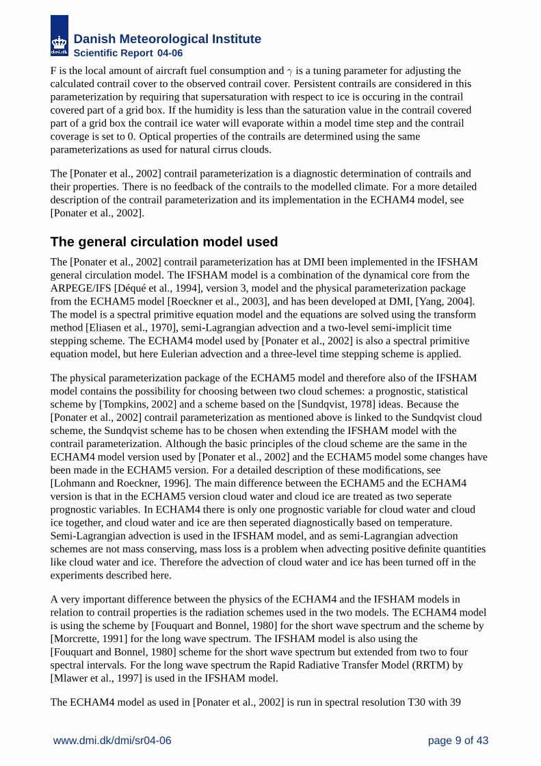
The contrail coverage of [Ponater et al., 2002] has been adjusted to observed contrail coverage forthe east Atlantic and western Europe area as determined in [Bakan et al., 1994]. Newer observations,[Meyer et al., 2001], indicate that the [Bakan et al., 1994] contrail cover may be a factor of two toolarge. Therefore some sensitivity experiments have been performed with a contrail coverage havinga global mean half the value of the global mean in the experiments described above. Table 3.1



Experiment Effective radius param. Optical depth SW forcing LW forcing Net forcing1 IFSHAM variable -1.4 1.5 0.12 ECHAM4 variable -1.8 2.0 0.23 12 µm 0.1 -3.4 5.3 1.94 12 µm 0.3 -7.7 14.5 6.75 12 µm 0.5 -11.4 22.0 10.6

Table 3.1: Global, annual mean of contrail radiative forcing (unit: mW/m2) for 5 sensitivityexperiments. Global mean of contrail coverage is 0.067 %. SW: short wave, LW: long wave

contains the results of the sensitivity experiments regarding radiative forcing of the contrails.

Experiment 1 and 2 are similar to the two experiments described in detail above. Experiment 1 isperformed with the standard version of IFSHAM and experiment 2 with the version of IFSHAMwhere the effective radius parameterization has been replaced by the one used in ECHAM4. Theonly difference to the above described experiments is that the contrail coverage is reduced by afactor of two. From table 3.1 it is seen that this reduction in contrail coverage implies a reduction bya factor of two in the radiative forcings. Experiment 3 to 5 are performed using constant values forthe effective radius (12 µm) and for the optical depth (0.1, 0.3 and 0.5 in the three experimentsrespectively) in the visible part of the spectrum. The optical depth of contrails as determined byIFSHAM is much smaller in the extratropics than these fixed values. Typically, the optical depth ofvisible contrails over Europe for example is 0.02-0.05. Using these relatively high, constant valuesfor the optical depth results in a considerable increase in short wave but especially in the long waveforcing, and therefore also the net forcing is increased substantially. These experiments are notexactly comparable to similar experiments in [Ponater et al., 2002] and [IPCC, 1999], but point inthe same direction, and the net forcing in these experiments is one to two orders of magnitude largerthan the net forcing determined in experiment 1 and 2. Figure 3.13 shows the geografical distributionof the net radiative forcing from experiment 3. It is seen that except in the tropics the net radiativeforcing is positive everywhere with maxima over Europe and the United States, a pattern similar tothe pattern shown in [IPCC, 1999], but in contrast to the pattern shown in figure 3.6.

It can be concluded from these experiments that the main difference between the radiative forcing asdetermined by the IFSHAM model and the ECHAM4 model is seen when the models are allowingfor contrails having variable optical depth with relatively small values in the extratropics, meaningthat the response of the radiation schemes in the two models to optically very thin ice clouds arequite different.

It is seen from these experiments that optical depth is a key parameter in determining the radiativeforcing of contrails and that also the effective radius have some impact. There is a huge uncertaintyin the determination of these two parameters, both in observations and in model simulations. Toinvestigate further the magnitude and geographical distribution of contrail optical depth and effectiveradius microphysical simulations with the MPC model have been performed and are described in thefollowing chapter.

The nudging techniqueAll general circulation models exhibit certain long term systematic errors when compared toobservations. One way to address the impact of these systematic errors on contrail behaviour is touse the nudging technique, [Jeuken et al., 1996]. When using this technique the model is forced



towards a reference data set, and when the reference data set represents observed data the systematicerrors of the model are minimized, because in each time step the model is following closely theobserved values of the prognostic variables. Nudging is a simple 4-dimensional assimilation of thereference data, where the prognostic model variables are relaxed towards the reference data:

Ψ(t + ∆t) = Ψ∗(t + ∆t) + ∆tΨREF (t + ∆t) − Ψ∗(t + ∆t)

τ(3.9)

The upper index ∗ indicates the preliminary prognostic variable just before nudging and the upperindex REF denotes the reference variable the model is relaxed towards. ∆t is the length of the timestep used in the model and τ is the relaxation time. The ECMWF Re-Analysis data (ERA-15)[Gibson et al., 1997] are used as the reference data towards which the model is relaxed. These dataare available every 6 hours in T106, L31 resolution. In order to use them for nudging they have to betruncated to the horizontal resolution used in the IFSHAM model (T63), and interpolated in thevertical to the orography-adjusted hybrid levels. As the relaxation towards the reference data is doneat every time step (in this case every 30 minutes) a cubic spline interpolation is used to obtainreference data at intermediate times. In practical use of the nudging technique the relaxation time τhas to be chosen carefully. If τ is too small noise and spin-up problems play an important role, but ifτ is too large the model is not following the reference data set closely. The variables assimilatedwere temperature, vorticity, divergence, logarithm of surface pressure, and the variables were nudgedin spectral space. The τ used was not the same for all the variables. The actual values were: 24h fortemperature, 6h for vorticity, 48h for divergence and 24h for logarithm of surface pressure. Theatmospheric humidity field was not nudged. The reason for this is that processes related to humiditycan act on a time scale smaller than 6 hours (the temporal resolution of the reference data set in thiscase) through threshold processes like condensation and deep convection. To avoid moisture spin-upproblems it therefore makes more sense to let the model develop its own humidity field. This isespecially important in the tropics where convection plays a large role. For a description of how thevalues for τ were determined see [Guldberg et al., 2004]

Impact of systematic errors on contrail behaviour in IFSHAMIn order to study the impact of systematic errors on contrail behaviour two sets of simulations havebeen performed with the IFSHAM model. In the first set - the control simulations - the model isforced with observed sea surface temperatures for ten winter seasons and 10 summer seasons in theperiod covered by the ERA-15 data set (1979-1993). In the second set - the nudged simulations - themodel is run in nudged mode and the model is relaxed towards observed data for the same 10 winterand summer seasons as in the control simulations. Also observed sea surface temperatures are usedin the nudged simulations. In the following averages over the 10 winter and the 10 summersimulations are shown and compared for the two sets of simulations. The contrail cover in thesesimulations are determined using the same calibration factor γ as used in the first experimentdescribed in this report, giving an annual mean contrail cover of 0.13 % as in [Ponater et al., 2002]for all contrails.

The IFSHAM model as compared to the ERA-15 data is generally too cold in most of theatmosphere in both summer and winter with the largest cold biases in the extratropical uppertroposphere and lower stratosphere - meaning at altitudes where most airplanes fly. Figure 3.14 isshowing the difference between the temperature at model level 10 of the control simulations and thenudged simulations for the winter (DJF) and the summer (JJA) season, and 3.15 is showing thedifference for model level 11. As the nudged simulations are following the ERA-15 data closely the



differences in figure 3.14 and 3.15 are in very good agreement with the systematic errors of themodel determined as the difference between the control simulations and the ERA-15 data. It is seenthat in winter the IFSHAM model is too cold almost everywhere on both levels. The largest biasesare seen at Antarctica and in the northern Pacific. In the summer season the model is too warm atAntarctica and too cold almost elsewhere. The largest cold biases are seen at northern high latitudes.The biases in the tropics are generally relatively small.

Figure 3.16 and 3.17 are equivalent to figure 3.14 and 3.15, but showing the relative humidity withrespect to ice. A general pattern is that the relative humidity in IFSHAM is too low a high latitudesand in the tropics whereas it is too high a midlatitudes (with some exceptions). It should be notedthat humidity is not nudged in these experiments, so the humidity in the nudged simulations isdetermined by the model based on close to observed values of the other prognostic variables.

Figure 3.18 is showing the ratio between the control and the nudged simulations of the total contrailcoverage. It is seen that the differences between the two model simulations to a large degree followthe pattern of the differences of the relative humidity, indicating that the relative humidity is likelythe determining factor for these differences. But in most areas the differences between the two modelsimulations are relatively small and the global mean of the contrail coverage is almost unchanged.

Figure 3.19 and 3.20 show the ratio between the control and the nudged simulations of ice waterpath and the optical depth, respectively, at level 11. Figure 3.21 show the differences between thecontrol and the nudged simulations for the effective radius at level 11. The differences in ice waterpath between the control and the nudged simulations are rather small, but there is a tendency of toolarge values in the tropics and too small values in the extratropics in the control simulations. As theeffective radius and the optical depth are determined from the ice water path, the same tendency isseen for the effective radius and the optical depth. Results for level 10 are not shown, as the generalpicture is the same as for level 11.

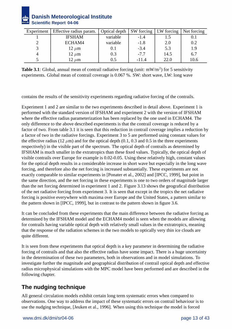
The main question is how the model biases affect the radiative forcing of contrails in the IFSHAMmodel. Figure 3.22 and 3.23 show the changes in short wave and long wave forcing. As the sign ofthe short wave forcing is negative positive values in the difference plot in figure 3.22 mean that themagnitude of the forcing is too low in the control simulations and this is the case almost everywherein winter. In summer the magnitude of the short wave forcing is too low over the northern part of theUnited States, the north Atlantic fligt corridor and northen Europe. In the southern part of the UnitedStates and southern Europe the magnitude of the forcing is too large in the control simulations. Inglobal mean the magnitude of the short wave forcing is increased by 0.4 mW/m2 in both summer andwinter when the model is nudged.

As seen in figure 3.23 the long wave forcing in the control simulations is too weak almosteverywhere in winter and too weak, respectively too strong in the areas where the short wave forcingis too weak, respectively too strong in summer. The global mean of the long wave forcing isincreased by 0.6 mW/m2, when the model is nudged.

Comparing figure 3.22 and 3.23 with the figures 3.19, 3.20 and 3.21 it is seen that the pattern ofchanges in the radiative forcings follows closely the pattern of changes of the ice water path and theoptical properties, meaning it is likely that the changes in radiative forcings can be explained by thechanges in these properties.

The net radiative forcing for the control and the nudged simulations is shown for winter in figure3.24 and for summer in figure 3.25. The net forcing in winter is approximately 25 % of the forcing insummer. The global mean of the net forcing is increased by 0.2 mW/m2 in both winter and summer



when the model is nudged. In winter the net forcing is increased by a factor of 4 from 0.07 to 0.3mW/m2. In summer the net forcing is changed from 0.8 to 1.0 mW/m2. Although the magnitude ofthe net forcing is changed the pattern of the forcing is to a large degree unchanged. It should benoticed that the negative net forcing over the United States is seen only in winter, not in summer.

As shown here the systematic errors have some impact on the radiavtive forcing of contrails - theincrease in the magnitude of the short and long wave forcing is 10-20 % when the model is nudgedas compared to the free simulation with the model. But the short wave and the long wave forcing isstill to a high degree cancelling each other resulting in a small net forcing an order of magnitude lessthan obtained by [Marquart and Mayer, 2002], and the pattern of the net forcing having areas withnegative values are not changed when the model is nudged.

[Marquart et al., 2003] has studied the impact of systematic errors on contrail coverage by off-linesimulations, but the systematic errors of the ECHAM4 model, especially regarding relative humidity,are somewhat different from the systematic errors of the IFSHAM model, and therefore the resultsare not directly comparable.

ConclusionsThe contrail parameterization of [Ponater et al., 2002] has been implemented in the IFSHAM modeland the contrail properties have been analyzed according to model dependency and impact of modelsystematic errors.

The magnitude of the contrail short wave forcing is larger than obtained by[Marquart and Mayer, 2002] and the contrail long wave forcing smaller. The resulting global meanof the contrail net forcing is an order of magnitude less than the [Marquart and Mayer, 2002]estimate. The net forcing shows areas over Europe and the United States with negative values. Thisis not seen by [Marquart and Mayer, 2002]. In their simulations the net forcing is positiveeverywhere.

Optical properties are important for the radiative impact of contrails. The magnitude andgeographical distribution of the effective radius is quite different in IFSHAM and ECHAM4.Replacing the effective radius parameterization of IFSHAM with the one from ECHAM4 has someimpact on the radiative forcing, but does not explain the main differences between IFSHAM andECHAM4.

IFSHAM experiments with fixed increased values of the optical depth at 0.1, 0.3 and 0.5 show asignificant change in the radiative forcing of the contrails, resulting in net forcings in betteragreement with other estimates and with positive net forcing everywhere (except for negative spotsin the tropics). But it is a question how realistic these values for the optical depth are.

The impact of the systematic errors of the model has been studied using the nudging technique. Thesystematic errors are causing a 10-20 % too low estimate of the short and long wave forcings. Thenet forcing is 75 % too low in winter and 20 % too low in summer in the control model compared tothe nudged version of the model. But the geographical distribution of the net forcing is unchanged.

In order to understand the differences in radiative forcing of contrails in the two models a detailedinvestigation of the differences in the radiation parameterizations for both long and short wave usedin the two models is needed. Also an analysis of the many different parameterizations of opticalproperties available could be of importance for the understanding the differnces seen with these twomodels.



The [Ponater et al., 2002] parameterization of contrails is only representing line-shaped contrails andnot cirrus clouds developed from these contrails. The contrail derived cirrus is likely to have a muchlarger radiative impact than the line-shaped contrails. DMI will participate in an EU-project,QUANTIFY, starting in 2005 and one of the obligations of DMI is to implement a parameterizationscheme in IFSHAM, describing the development of line-shaped contrails into cirrus clouds.Furthermore nudging experiments with IFSHAM in high resolution, T159 and 60 vertical layers,will be performed and compared with analyses of satellite images. Especially the very high verticalresolution is likely important for the representation of contrails and contrail derived cirrus.



Figure 3.1: Annual mean of total contrail coverage (% )

Figure 3.2: Annual mean of contrail coverage (% ) at model level 10 (∼ 210 hPa)

Figure 3.3: Annual mean of contrail coverage (% ) at model level 11 (∼ 240 hPa)



Figure 3.4: Annual mean of contrail short wave forcing at TOA (mW/m2)

Figure 3.5: Annual mean of contrail long wave forcing at TOA (mW/m2)

Figure 3.6: Annual mean of contrail net forcing at TOA (mW/m2)



Figure 3.7: Annual, conditional mean of the ice water path for contrails at level 10 (left) and level11 (right) (g/m2)

Figure 3.8: Annual, conditional mean of the optical depth for contrails at level 10 (left) and level 11(right).

Figure 3.9: Annual, conditional mean of the effective radius for contrails at level 10 (right) and level11 (left) (µm).



Figure 3.10: Annual, conditional mean of the optical depth for contrails at level 10 (left) and level11 (right). - ECHAM4 effective radius

Figure 3.11: Annual, conditional mean of the effective radius for contrails at level 10 (right) andlevel 11 (left) (µm). - ECHAM4 effective radius

Figure 3.12: Annual mean of contrail net forcing at TOA (mW/m2) - ECHAM4 effective radius



Figure 3.13: Annual mean of contrail net forcing at TOA (mW/m2) - Optical depth: 0.1



Figure 3.14: Ten-year mean differences of temperature between control and nudged simulations atlevel 10 for DJF (left) and JJA (right) (K)

Figure 3.15: Ten-year mean differences of temperature between control and nudged simulations atlevel 11 for DJF (left) and JJA (right) (K)

Figure 3.16: Ten-year mean differences of relative humidity with respect to ice between control andnudged simulations at level 10 for DJF (left) and JJA (right) (%)

Figure 3.17: Ten-year mean differences of relative humidity with respect to ice between control andnudged simulations at level 11 for DJF (left) and JJA (right) (%)



Figure 3.18: Ratio between control and nudged simulations of ten-year mean of total contrailcoverage for DJF (left) and JJA (right)

Figure 3.19: Ratio between control and nudged simulations of ten-year mean of ice water path atlevel 11 for DJF (left) and JJA (right)

Figure 3.20: Ratio between control and nudged simulations of ten-year mean of optical depth atlevel 11 for DJF (left) and JJA (right)

Figure 3.21: Ten-year mean differences of effective radius between control and nudged simulationsat level 11 for DJF (left) and JJA (right) (µm)



Figure 3.22: Ten-year mean differences of short wave radiative forcing between control and nudgedsimulations for DJF (left) and JJA (right) (mW/m2)

Figure 3.23: Ten-year mean differences of long wave radiative forcing between control and nudgedsimulations for DJF (left) and JJA (right) (mW/m2)

Figure 3.24: Ten-year mean of net radiative forcing for control (left) and nudged simulations (right)for DJF (mW/m2)

Figure 3.25: Ten-year mean of net radiative forcing for control (left) and nudged simulations (right)for JJA (mW/m2)



Microphysical simulations of spreading contrails

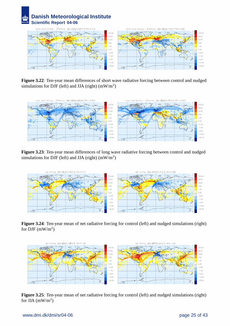
MotivationThe climatological impact of contrails and contrail-derived cirrus clouds depends on microphysicalproperties of these types of clouds. That is, the size distribution and shapes of the particles, the icewater content and of course the spatial formation of the clouds. All these characteristics change intime as a cloud evolves, and they depend on the local environment. The growth of airplane contrailsinto cirrus clouds is mainly controlled by initial humidity, wind shear, temperature and radiativeheating caused by interaction of ice particles with infrared radiation.

Figure 4.1: Example of a MPC contrail simulation (afternoon March 16 2003, eastern Denmark).Wind, temperature and pressure was taken from ECMWF (European Centre for Medium-RangeWeather Forecast) in this simulation, while the humidity was initiated with values from local radiosoundings. Looking through the cloud one sees the integrated cross section area, which gives a goodimpression of the physical distribution of the cloud. From [Nielsen, 2004].

Ground LIDAR observations [Larchevêque et al., 2002, Del Guasta and Niranjan, 2001] and airplaneobservations [Jensen et al., 1998, Heymsfield et al., 1998, Lawson et al., 1998, Schröder et al., 2000]of developing contrails provides information about contrail-cirrus optical properties, humidity andparticle distributions. The drawback of these observations is that it is hard to track a cloud history,since observations are restricted to a vertical profile at a given location or a single point at a giventime. In order to establish a relation between the cloud properties and the conditions at the pointwhere the cloud was created, it is necessary to follow the history of a specific cirrus cloud. This canbe done by satellite observations. Observations of contrail cirrus by satellite images has beeninvestigated by [Mannstein and Schumann, 2004, Minnis et al., 1998]. A problem with satelliteobservations is to separate contrails from ordinary cirrus clouds as they become more and moresimilar during the lifetime of a contrail. Furthermore satellite observations does not provide detailedinformation of local humidity in the contrail and its surroundings.



It is therefore desirable to perform detailed cloud resolving and microphysical modeling of contrailsin order to get information about their temporal and spatial development, and their microphysicalproperties. This has been done for a special case by [Jensen et al., 1998] in the SUCCESS campaign,and here the thread off that study is taken up with the purpose of comparing microphysicalsimulations to the global climate model IFSHAM.

Simulation methodThe MicroPhysical Cirrus (MPC) model is an integrated model, developed at DMI, which combinesa well tested microphysical box-model with a quite accurate 3-D advection scheme. Themicrophysical kernel was originally developed for simulations of PSC clouds ([Larsen, 2000]), andas a consequence the MPC-model may be applied on PSC-clouds as well as cirrus clouds. Thedynamical variables of the model are gas-phase mixing ratios of water and HNO3, size-distributionsof 4 different particle types, (supercooled ternary solutions, sulphuric acid tetrahydrate, nitric acidtrihydrate and ice) and in-particle weight fractions of condensed phase constituents. The modelincludes nucleation and deposition-processes and detailed sedimentation calculation on each sizebin. Wind transport, sedimentation and parts of the particle growth processes are calculated by theWalcek-algorithm [Walcek, 2000].

The model is linked with optical routines enabling extinction coefficients and backscattering ratios tobe calculated. The software is flexible, in the sense that a lot of parameters is specified as input, andtherefore it is easy to change e.g. dimensions, location, processes, initialization, output etc. Themodel is running off line, meaning that it does not include dynamical feedback fromcloud-processes; the wind/temperature and pressure history has to be given beforehand. Modules hasbeen written facilitating this to be done in several ways, e.g. by loading ECMWF fields into themodel, generating fields from radio soundings (as in figure 4.1), or by constructing artificial fieldsfor theoretical analysis (as in figure 4.4).

Simulations aims and setupThe purpose of the simulations described here is to compare the MPC-models predictions ofcontrail-cirrus cloud effective radius and optical depth, with the corresponding parameters of theIFSHAM model. To establish this comparison MPC simulations are done in an environmentresembling the wintertime conditions in North Atlantic flight corridor. Information about theseconditions cannot be retrieved from ECMWF, since the ECMWF relative humidity with respect toice is restricted to below 100 %. Instead UTLS profiles are retrieved from radio soundings in (andnear) the North Atlantic. The reason for choosing the North Atlantic region is that it is an area withrelatively large and homogeneous flight load.

Analysis of radio soundings

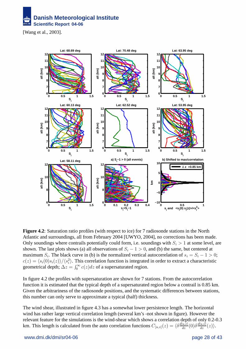
Radio soundings from 7 different stations around the North Atlantic were retrieved from theWyoming database [UWYO, 2004]. The chosen data-set includes all soundings from February 2004.In figure 4.2 profiles of the saturation ratio with respect to ice, Si, are plotted for all stations, in thecases where supersaturation occurs somewhere between 8 and 12 km altitude. An autocorrelationfunction is formed from the parts of profiles exceeding Si = 1, and this function is used to calculatea typical length depth ∆z of a supersaturated region below an arbitrary positioned contrail. It shouldbe noted that ∆z is probably an underestimate for two reasons: First, the supersaturated regions hasa tendency to occur in the lower part of the flight corridor, causing a bigger likelihood for the contrailto appear in the upper part of the supersaturated region, and secondly the RS80 humicap radiosonde,which presumably has been used, are known to underestimate humidities near the tropopause



[Wang et al., 2003].

0 0.5 1 1.56

7

8

9

10

11

12

alt

(km

)

Si

Lat: 68.69 deg

0 0.5 1 1.56

7

8

9

10

11

12

alt

(km

)S

i

Lat: 70.48 deg

0 0.5 1 1.56

7

8

9

10

11

12

alt

(km

)

Si

Lat: 63.95 deg

0 0.5 1 1.56

7

8

9

10

11

12

alt

(km

)

Si

Lat: 60.13 deg

0 0.5 1 1.56

7

8

9

10

11

12

alt

(km

)

Si

Lat: 62.52 deg

0 0.5 1 1.56

7

8

9

10

11

12

alt

(km

)S

i

Lat: 53.95 deg

0 0.5 1 1.56

8

10

12

alt

(km

)

Si

Lat: 58.11 deg

0 0.1 0.2 0.3 0.46

8

10

12

alt

(km

)

si=S

i−1

a) Si−1 > 0 (all events)

0 0.5 1−10

−5

0

5

10 b) Shifted to max/correlation

km

si and <s

i(0) s

i(z)>/<s

i2>

∆ z =0.85 km

Figure 4.2: Saturation ratio profiles (with respect to ice) for 7 radiosonde stations in the NorthAtlantic and surroundings, all from February 2004 [UWYO, 2004], no corrections has been made.Only soundings where contrails potentially could form, i.e. soundings with Si > 1 at some level, areshown. The last plots shows (a) all observations of Si − 1 > 0, and (b) the same, but centered atmaximum Si. The black curve in (b) is the normalized vertical autocorrelation of si = Si − 1 > 0;c(z) = 〈si(0)si(z)〉/〈s2

i 〉. This correlation function is integrated in order to extract a characteristicgeometrical depth; ∆z =

∫

∞

0 c(z)dz of a supersaturated region.

In figure 4.2 the profiles with supersaturation are shown for 7 stations. From the autocorrelationfunction it is estimated that the typical depth of a supersaturated region below a contrail is 0.85 km.Given the arbitrariness of the radiosonde positions, and the systematic differences between stations,this number can only serve to approximate a typical (half) thickness.

The wind shear, illustrated in figure 4.3 has a somewhat lower persistence length. The horizontalwind has rather large vertical correlation length (several km’s -not shown in figure). However therelevant feature for the simulations is the wind-shear which shows a correlation depth of only 0.2-0.3km. This length is calculated from the auto correlation functions C[u,v](z) = 〈δ d[u,v]

dz(0)δ d[u,v]

dz(z)〉.



0 0.2 0.4 0.6 0.8 1−1

−0.8

−0.6

−0.4

−0.2

0

0.2

0.4

0.6

0.8

1

(km

)

mean normalized correlation coef.

∆ zu =0.25 km

∆ zv =0.23 km

0 20 40 60 80 10010

−5

10−4

10−3

10−2

10−1

100

|du/dz| and |dv/dz| m/(s km)

PD

F, s

km

/m

⟨ |d [u,v]/dz| ⟩ = 7.2 (m/skm)

200 220 240 2600

10

20

30

40

Ttropopause

(K)

#/b

in

⟨ Ttropo

⟩ = 215 (K)

200 220 240 2606

8

10

12

Ttropopause

(K)

alt tr

op

op

ause

(km

)

−10 −5 0 56

7

8

9

10

11

12

lapse rate dT/dz (K/km)

alt (

km)

100 200 300 400 500

p (hPa)

Figure 4.3: From left, 1: Probability density distribution of shear rate from the soundings of figure4.2. 2: Averaged auto correlation functions indicating the vertical persistence of a given sheartendency (see text). 3: Histogram of tropopause temperatures, and scatter plot of tropopausetemperature versus tropopause height. 4: Lapse rate and pressure profiles.

The shear can reach values up to hundreds of m/(s km) in narrow regions, while the mean value isonly 7.2 m/(s km). Since the statistics of meridional and longitudinal wind-shear are almost identicalwe assume that the contrail spreading does not have a “preferred direction” in this area. Since thedirections are arbitrary the wind statistics of figure 4.3 represents wind statistics projectedorthogonally to an arbitrary oriented contrail. In figure 4.3, temperature characteristics are alsoshown.

Baseline simulation and variations

From the observations a baseline simulation is formed. The characteristics of initialization of thissimulation is shown in table 4.1. In addition to the baseline simulation a set of single parametervariations is chosen, in order to examine the contrail characteristics dependency of differentparameters. All cases are supersaturated and fulfills the requirements for contrail formation andpersistence, so the outcome is a conditional characterization; if the conditions for contrails are there,how will they develop in time, and what are their optical properties. The MPC model is not able tosimulate the initial turbulent phase, i.e the part where the vortices dies out, and where nucleationoccurs. The dynamics of this phase has been simulated e.g. in [Gierens and Jensen, 1998]. Based onthese simulations, and on comparison with measurements [Schröder et al., 2000], the initial width,height and particle size-distribution are chosen, in order to approximate a 15 minutes old contrail.

ResultsIn the simulations presented here the MPC model is executed in 2-d mode, with periodic boundaryconditions horizontally. Due to the physical nature of contrail spreading it is not necessary to run in3-d. The simulations includes a “baseline-simulation”, representing a typical contrails event. Theaccuracy of the baseline simulation has been tested with additional simulations with higherresolution, see 4.1. Low vertical resolution results in an apparent horizontal “wave” in the opticaldepth, which is identified as a result of different advection velocities of different layers. This effectdoes not lead to any error in the integrated clod parameters. Several additional simulations have beenperformed, all representing variations in the model input or simulation parameters, chosen to test thesensitivity of contrail formation.



Baseline VariationsSaturation Ratio 1.25 1.1Wind shear 7.2m/(s km) 12.0 (90 deg )Shear depth 0.25 km 0.45 kmSupersaturation depth 0.8 kmTemperature 215 K at 9.5 km 224 K at 9.5 km and 216 K at 11.5 kmTropopause/contrail height 9.5 km 10.5 kmLapse 7.0 m/s km 9.8 m/s kmInitial particle density 20/cm3 100/cm3

Initial contrail width/height 400m/100m 800m/200mInitial mean particle radius 2 µ m 10 µ m)Initial log-normal stdv 1.25Ice water sticking coeff. 1.0 0.05Ice particle aspect ratio 1.11Grid Resolution 66m × 19m 40m × 19m and 66m ×6.3m

Table 4.1: Properties of the baseline simulation. Last column are the variations chosen forsensitivity tests. “Shear depth” and “supersaturation depth” indicates the depth of the layer below thecontrail, where these properties persists, before they are truncated. In table 4.2 the simulationdenoted “216 K at 11.5 km” is refered to as “Tropical”.

Features of the baseline simulation

Generally the total number of particles is decreasing moderately during the first 2 hours, while thecontrail is spreading. The size distributions varies a lot in space, with the larger particles (order of 40µ m) at the bottom of the cloud and the smaller particles at top (see figure 4.4 (1)).



km

(1)

0 5 10 15 207

8

9

10

Ri,e

ff µ

m

10

20

30

40

0.50.5

0.5

1 1

1

1.522.53

(2)

0 5 10 15 207

8

9

10

Si

0.95

1

1.05

1.1

1.15

1.2

km

km

(3)

0 5 10 15 207

8

9

10

Ext

inct

ion

(55

0nm

) m

−1

5

10

15

x 10−4

km

(4)

0 5 10 15 207

8

9

10

Par

ticl

e n

um

ber

den

sity

cm

−3

1

2

3

4

5

Sim. id: bhr2, Contrail age = 120 min

Figure 4.4: Features of the baseline simulation. Black contours in first plot denotes ice water content(mg/m3)



The number density remains fairly high, i.e. up to 8 particles per cm3 at the cloud top even after 2hours of existence. The total ice water content (IWC) also has its maximum at the cloud top.However, the IWC is growing to 1 mg/m3 in the fall streak, even though the number density is verylow there. This leads to a relative small but significant contribution to the extinction coefficient andoptical depth of the cloud 8-10 kilometers from the contrail core. In figure 4.5 the vertical opticaldepth across the contrail is plotted at different times. The optical depth is very low, starting at around0.11 at time = 0 h, decreasing to 0.02-0.03 after two hours.

0 2 4 6 8 10 12 14 16 18 200

0.02

0.04

0.06

0.08

0.1

0.12

length (km)

Op

tica

l Dep

th

0.00027778

0.4

0.8

1.2

1.6

2

time (h)

Figure 4.5: Vertical baseline optical depth of scattering at 550 nm.

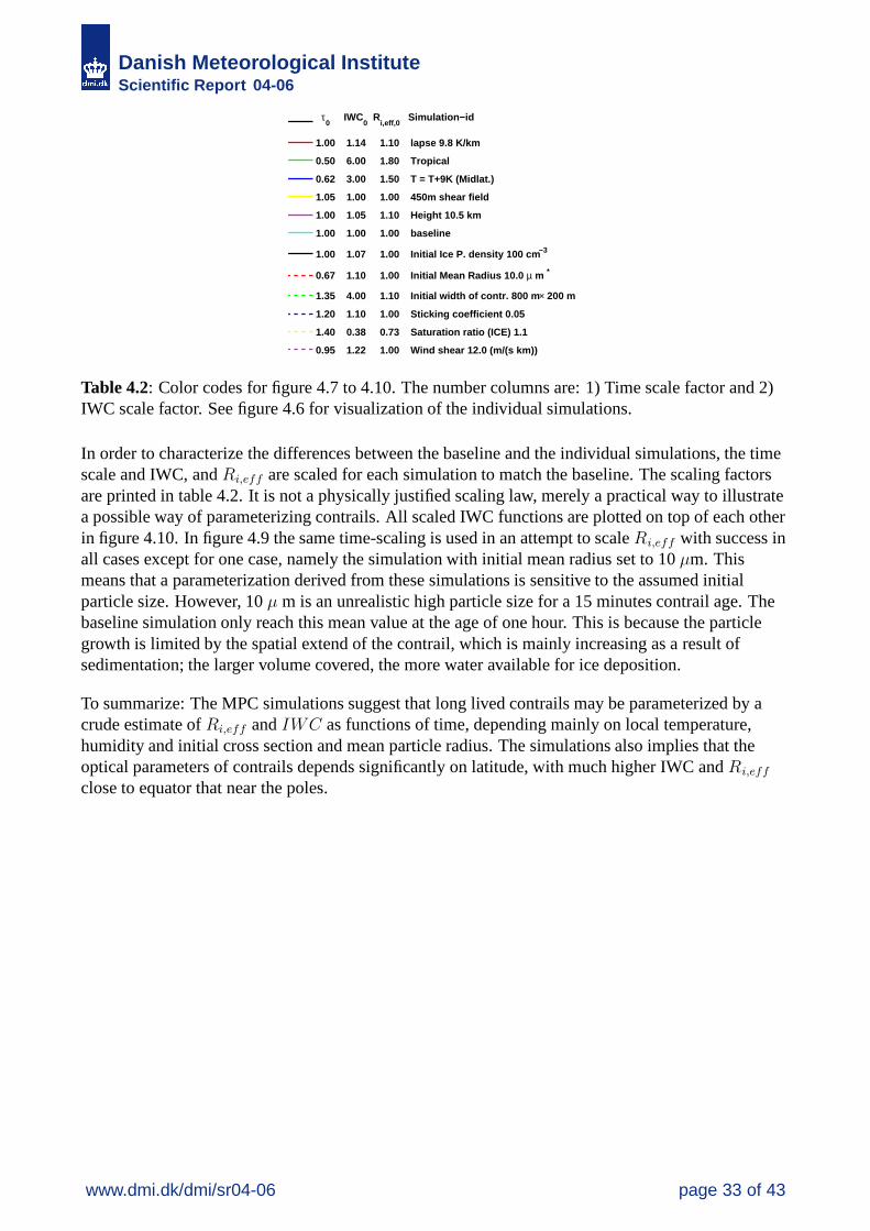
Features of variation ensemble.

In addition to the baseline simulation, 11 other simulations are presented. Short descriptions of thesimulations are found in table 4.2. In order to overview the differences between variousperturbations a few feature variables are defined: The total ice water cross section i.e. the IWC perunit length along the contrail is calculated by integrating IWC over the contrail cross section. Seefigure 4.7. Three simulations are strikingly different from the main group: Si = 1.1 givessignificantly smaller IWC. The T = T + 9 K simulation and the “Tropical” simulation which isperformed with T = 230 K at flight altitude, gives much higer IWC.

Likewise a variable, “the total extinction” ,W , is defined by integrating the optical depthhorizontally. It’s dimension is length. And even though W doesn’t represent the actual geometricalwidth of the contrail, it can give an idea about the overall impact of the contrail. W is plotted asfunction of time in figure 4.8. Again the tropical simulation gives high numbers. The red dashedcurve is a contrail which is initiated which much bigger ice crystals (10 µ) and consequently it hashigher extinction coefficient from the beginning. Finally the mean effective radius Ri,eff weightedwith IWC is calculated as function of time and plotted in figure 4.9. Here the same pattern is seen.The tropical simulation stabilizes at Ri,eff = 45 − 47µm in one hour, in contrast to the baselinewhich reaches a value around 17 µm in one hour.



τ0 IWC

0 R

i,eff,0 Simulation−id

1.00 1.14 1.10 lapse 9.8 K/km

0.50 6.00 1.80 Tropical

0.62 3.00 1.50 T = T+9K (Midlat.)

1.05 1.00 1.00 450m shear field

1.00 1.05 1.10 Height 10.5 km

1.00 1.00 1.00 baseline

1.00 1.07 1.00 Initial Ice P. density 100 cm −3

0.67 1.10 1.00 Initial Mean Radius 10.0 µ m *

1.35 4.00 1.10 Initial width of contr. 800 m× 200 m

1.20 1.10 1.00 Sticking coefficient 0.05

1.40 0.38 0.73 Saturation ratio (ICE) 1.1

0.95 1.22 1.00 Wind shear 12.0 (m/(s km))

Table 4.2: Color codes for figure 4.7 to 4.10. The number columns are: 1) Time scale factor and 2)IWC scale factor. See figure 4.6 for visualization of the individual simulations.

In order to characterize the differences between the baseline and the individual simulations, the timescale and IWC, and Ri,eff are scaled for each simulation to match the baseline. The scaling factorsare printed in table 4.2. It is not a physically justified scaling law, merely a practical way to illustratea possible way of parameterizing contrails. All scaled IWC functions are plotted on top of each otherin figure 4.10. In figure 4.9 the same time-scaling is used in an attempt to scale Ri,eff with success inall cases except for one case, namely the simulation with initial mean radius set to 10 µm. Thismeans that a parameterization derived from these simulations is sensitive to the assumed initialparticle size. However, 10 µ m is an unrealistic high particle size for a 15 minutes contrail age. Thebaseline simulation only reach this mean value at the age of one hour. This is because the particlegrowth is limited by the spatial extend of the contrail, which is mainly increasing as a result ofsedimentation; the larger volume covered, the more water available for ice deposition.

To summarize: The MPC simulations suggest that long lived contrails may be parameterized by acrude estimate of Ri,eff and IWC as functions of time, depending mainly on local temperature,humidity and initial cross section and mean particle radius. The simulations also implies that theoptical parameters of contrails depends significantly on latitude, with much higher IWC and Ri,eff

close to equator that near the poles.



km

lapse 9.8 K/km

0 5 10 15 20

8

10

µ m20

400.5 0.51 1

1

1.5

Tropical

0 5 10 15 20

8

10

µ m

20406080

11

122

2 22333

44

5 5667

T = T+9K (Midlat.)

0 5 10 15 20

8

10

µ m

204060

0.50.51

111.51.51.5

222 2.52.5

33.54 4

450m shear field

0 5 10 15 20

8

10

µ m20

400.50.51 1.5

Height 10.5 km

0 5 10 15 20

8

10

µ m20

400.50.5 1 11.5

baseline

0 5 10 15 20

8

10

µ m20

400.5 0.5

0.51

1

Initial Ice P. density 100 cm−3

0 5 10 15 20

8

10

µ m20

400.50.5

0.51 11

1.5

Initial Mean Radius 10.0 µ m *

0 5 10 15 20

8

10

µ m20

400.50.5

11 1.51.5 22.5

Initial width of contr. 800 m× 200 m

0 5 10 15 20

8

10

µ m20

400.50.5

0.511 11

1.51.5 1.522 222.5

Sticking coefficient 0.05

0 5 10 15 20

8

10

µ m20

400.50.5 1 1

11.5

Saturation ratio (ICE) 1.1

0 5 10 15 20

8

10

µ m

102030

0.20.20.20.4 0

.40.6

Wind shear 12.0 (m/(s km))

0 5 10 15 20

8

10

µ m20

400.2

0.20.2

0.20.40.4

0.4

0.6

0.6 0.6 0.60.8 0.80.81 11

1 11 1 1

km

Figure 4.6: IWC (black contours units: mg/m3) and Ri,eff (color-scale) of 12 different simulations.The coordinate units are km.



0 0.1 0.2 0.3 0.4 0.5 0.6 0.7 0.8 0.9 110

−7

10−6

10−5

Time (h)

Co

ntr

ail I

CE

wat

er (

kg/m

)

Figure 4.7: Total contrail ice water content [kg/m] as function of time

0 0.2 0.4 0.6 0.8 1 1.2 1.4 1.6 1.8 20

0.2

0.4

0.6

0.8

1

1.2

1.4

1.6

1.8

2

Time (h)

To

tal e

xtin

ctio

n a

t 55

0 n

m (

km)

Figure 4.8: Total extinction at 550 nm . The descriptions are found in table 4.2



0 0.2 0.4 0.6 0.8 1 1.2 1.4 1.6 1.8 20

5

10

15

20

25

30

35

40

45

50

Time (h)

Ri,e

ff, w

eig

hte

d w

ith

IWC

(µ m

)

Figure 4.9: Effective radius weighted by IWC [µ m]

0 0.5 1 1.5

10−6

Time/τ0

Co

ntr

ail I

CE

wat

er /I

WC

0

Scaled Total Ice Water

Figure 4.10: Scaled total contrail ice water content as function of scaled time.



0 0.5 1 1.5 2 2.5 3 3.5 410

0

101

102

Scaled Time

Ri,e

ff /R

i,eff

,0

Scaled Ri,eff

Figure 4.11: Scaled effective radius as function of scaled time.The simulation with initial meanradius = 10 µm does not obey the scaling law. I.e., it is not possible to reduce the time scale forRi,eff and IWC with the same constant, τ , see text.



ConclusionsThe physical properties of contrails has been studied through microphysical simulations featuringthe interplay between size distributions, sedimentation, shear, deposition, sublimation etc.

Simulations of contrail events in 12 different situations, surrounding a baseline simulation,resembling a typical winter profile of the north Atlantic at approximately 60deg latitude were run for2 hours.

The optical depth at 0.55 µ m decreases from 0.11 to 0.05 in the first hour of simulation. Generallythe optical depth is largest in the contrail core. The fall streaks has an optical depth below 0.02, butaround 2 hours into the simulation it increases to above 0.02, and approaches the optical depth of thecontrail core, around 0.03.

The sensitivity studies was used to extract empirical scaling relations, for the time dependenteffective radius and ice water content, suggesting a route for parameterization of contrailsdeveloping into cirrus clouds.

The largest sensitivity is observed on changes in humidity, temperature and wind shear. Humidityand temperature essentially acts through the same mechanism; since contrails is formed when therelative humidity is around 100 % and above, and since absolute humidity increases fast withtemperature, larger temperatures usually corresponds to larger amounts of water vapor available fordepositional growth.

The effective radius is doubled, from around 16 µm at after 1 hour, to around 32 µm if the contrailcore temperature is increased 9 K from 215 K to 224 K, and up to 45-47 µm if the temperature israised to 230 K. The same variable is decreased from 16 µm to 7 µm if the initial relative humidity isset to 110% instead of 125%.

Change of wind shear does not influence much on effective radius or ice water content during the 2hour simulation, but the horizontal width of the contrail increases with the wind shear. A wind shearrate of 7.2 m/(s km), which is the average magnitude around the tropopause in the north Atlanticresults in a smearing to approximately 5 km after 1 hour.



Discussion and ConclusionsComparison between MPC and IFSHAMThe contrail parameterization employed in IFSHAM is based on satellite observations of linear, i.e.young contrails. Disregarding the fact that older contrails has greater impact according to the MPCmodel, we shall restrict the comparison to younger contrails. The IFSHAM winter mean opticaldepth in the north Atlantic is between 0.02 and 0.05, which is less than the prediction of the MPCbaseline simulation; assuming that the contrails are less than one hour old, the MPC baselinesimulation predicts optical depth to be 0.05 to 0.11 during the first hour. However, in the nudgedIFSHAM simulations (where the model systematic errors are minimized) the winter mean of theoptical depth in the north Atlantic is between 0.02 and 0.1 and therefore corresponds better to theMPC baseline simulation. In the MPC simulations, the optical depth is very sensitive to initialhumidity, and the simulation with Si = 1.1 predicts smaller optical depth values than the baselinesimulation. (Initialization of the humidity in the MPC simulations was based on radio-soundings,which are not reliable near the tropopause.)

The winter mean of the effective radius of particles in the north Atlantic UTLS, as predicted byIFSHAM lies in the area of 14-17 µm, whereas the ECHAM4 model predicts average radii in theinterval 12-13 µm. The mean of MPC effective radius from the same period is lower. This may haveto do with the initialization of MPC; the test run initialized with larger particles (r = 10µm) actuallylies above the IFSHAM values. After 1.3 hour the effective radius difference between the two MPCinitializations vanishes.

The MPC simulations with larger temperatures illustrates what happens in the tropics: The highertemperatures leads to more excess water, and bigger effective radii. This is also captured byIFSHAM, but this feature is absent in the average values predicted by the ECHAM4parameterization. Specifically in the 230 K simulation, which corresponds to a tropical profile theeffective radius increases from 2 to almost 50 µm, which is consistent with average values of 20-25µm as determined by IFSHAM in the tropical regions.

So in terms of variability and latitude dependency IFSHAM and MPC are consistent, while theECHAM4 parameterization has a much smaller latitude dependency.



References

[Appleman, 1953] Appleman, H. (1953). The formation of exhaust condensation trails by jetaircraft. Bull. Am. Meteorol. Soc., 34:14–20.

[Bakan et al., 1994] Bakan, S., Gothe, M. B., Gayler, V., and Grassl, H. (1994). Contrail frequencyover Europe from NOAA-satellite images. Ann. Geophys., 12:962–968.

[Del Guasta and Niranjan, 2001] Del Guasta, M. and Niranjan, K. (2001). Observation oflow-depolarization contrails at Florence (Italy) using a 532-1064 nm polarization LIDAR.Geophysical Research Letters, 28:4067–4070.

[Déqué et al., 1994] Déqué, M., Dreveton, C., Braun, A., and Cariolle, D. (1994). The arpege/ifsatmosphere model: a contribution to the french community climate modelling. ClimateDynamics, 10:249–266.

[Eliasen et al., 1970] Eliasen, E., Machenhauer, B., and Rasmussen, E. (1970). On a numericalmethod for integration of the hydrodynamical equations with a spectral representation of thehorizontal fields. Report no. 2. Institute for Theoretical Meteorology, Copenhagen University,Copenhagen, Denmark.

[Fortuin et al., 1995] Fortuin, J. P. F., van Dorland, R., Wauben, W. M. F., and Kelder, H. (1995).Greenhouse effect of of aircraft emissions as calculated by a radiative transfer model. Ann.Geophys., 13:413–418.

[Fouquart and Bonnel, 1980] Fouquart, Y. and Bonnel, B. (1980). Computations of solar heating ofthe earth’s atmosphere: A new parameterization. Beitr. Phys. Atmos., 53:35–62.

[Gibson et al., 1997] Gibson, J. K., Kå llberg, P., Uppala, S., Hernandez, A., Nomura, A., andSerrano, E. (1997). ERA-15 Description, volume 1 of ECMWF Re-analysis Project Report Series.ECMWF, Reading, U.K.

[Gierens and Jensen, 1998] Gierens, K. and Jensen, E. (1998). A numerical study of thecontrail-to-cirrus transition. Geophysical Research Letters, 25(23):4341–4.

[Guldberg et al., 2004] Guldberg, A., Kaas, E., Deque, M., Yang, S., and Thorsen, S. V. (2004).Reduced systematic errors by empirical model correction; impact on seasonal prediction skill .Tellus A. Accepted.

[Heymsfield et al., 1998] Heymsfield, A. J., Lawson, R. P., and Sachse, G. W. (1998). Growth of icecrystals in a precipitating contrail. Geophysical Research Letters, 25:1335–1338.

[IPCC, 1999] IPCC (1999). Aviation and the global atmosphere. Cambridge University Press,Cambridge, UK.

[Jensen et al., 1998] Jensen, E. J., Ackerman, A. S., Stevens, D. E., Toon, O. B., and Minnis, P.(1998). Spreading and growth of contrails in a sheared environment. jgr, 103(.12):31557–31568.

[Jeuken et al., 1996] Jeuken, A. B. M., Siegmund, P. C., Heijboer, L. C., Feichter, J., and Bengtsson,L. (1996). On the potential of assimilating meteorological analyses in a global climate model forthe purpose of model validation. J. Geophys. Res., 101:16939–16950.



[Larchevêque et al., 2002] Larchevêque, G., Balin, I., Quaglia, P., Nessler, R., Simeonov, V., vanden Bergh, H., and Calpini, B. (2002). Optical Properties of Aerosols - Clouds - Contrails andWater Vapor Mixing Ratio By Lidar From The Jungfraujoch Research Station (3580 M Asl). EGSXXVII General Assembly, Nice, 21-26 April 2002, abstract #5820, 27:5820–+.

[Larsen, 2000] Larsen, N. (2000). Polar stratospheric clouds - microphysical and optical models.Tecnical Report, DMI, 00-06.

[Lawson et al., 1998] Lawson, R., Heymsfield, A., Aulenbach, S., and Jensen, T. (1998). Shapes,sizes and light scattering properties of ice crystals in cirrus and a persistent contrail duringSUCCESS. Geophysical Research Letters, 25(9):1331–4.

[Lohmann and Roeckner, 1996] Lohmann, U. and Roeckner, E. (1996). Design and performance ofa new cloud microphysics scheme developed for the echam general circulation model. ClimateDynamics, 12:557–572.

[Mannstein and Schumann, 2004] Mannstein, H. and Schumann, U. (2004). Observations ofContrails and Cirrus over Europe. In Robert Sausen, C. F. and Amanatidis, G., editors, "Aviation,Atmosphere and Climate", number 83 in Air pollution research report, pages 244–248. EuropeanCommission.

[Marquart, 2003] Marquart, S. (2003). Klimawirkung von Kondensstreifen: Untersuchungen miteinem globalen atmosphaerischen Zirkulationsmodell. Dissertation der Fakultaet fur Physik derLudwig-Maximilians-Universitae Munchen. Deutsches Zentrum fur Luft- und Raumfahrt.,Oberpfaffenhofen, Germany.

[Marquart and Mayer, 2002] Marquart, S. and Mayer, B. (2002). Towards a reliable GCMestimation of contrail radiative forcing. Geophysical Research Letters, 29:20–1–20–4.

[Marquart et al., 2003] Marquart, S., Ponater, M., Mager, F., and Sausen, R. (2003). FutureDevelopment of Contrail Cover, Optical Depth, and Radiative Forcing: Impacts of Increasing AirTraffic and Climate Change. Journal of Climate, 16:2890–2904.

[Meerkotter et al., 1999] Meerkotter, R., Schumann, U., Doelling, D. R., Minnis, P., Nakajima, T.,and Tsushima, Y. (1999). Radiative forcing by contrails. Ann. Geophys., 17:1080–1094.

[Meyer et al., 2001] Meyer, R., Mannstein, H., and Wendling, P. (2001). Regional Frequency ofContrails Derived from Satellite Data and their Radiative Forcing. In Schumann, U. andAmanatidis, G., editors, "Aviation, aerosols, contrails and cirrus clouds", number 74 in Airpollution research report, pages 230–234. European Commission.

[Minnis et al., 2004] Minnis, P., Kirk Ayers, J., Palikonda, R., and Phan, D. (2004). Contrails, cirrustrends, and climate. Journal of Climate, 17:1671–1685.

[Minnis et al., 1998] Minnis, P., Young, D. F., Garber, D. P., Nguyen, L., Smith, W. L., andPalikonda, R. (1998). Transformation of contrails into cirrus during SUCCESS. GeophysicalResearch Letters, 25:1157–1160.

[Minnis et al., 1999] Minnis, P. Schumann, U., Doelling, D. R., Gierens, K. M., and Fahey, D.(1999). Global distribution of contrail radiative forcing. Geophysical Research Letters,26:1853–1856.

[Mlawer et al., 1997] Mlawer, E. J., Taubman, S. J., Brown, P. D., Ianoco, M. J., and Clough, S. A.(1997). Radiative transfer for inhomogenous atmospheres: Rrtm, a validated correlated-k modelfor the longwave. Journal of geophysical research, 102:16663–16682.



[Morcrette, 1991] Morcrette, J.-J. (1991). Radiation and cloud radiative properties in the europencentre for medium range weather forecasts forecasting system. J. Geophys. Res., 96:9121–9132.

[Nielsen, 2004] Nielsen, J. K. (2004). 3-D simulation of contrail to cirrus transition, - the onset ofsedimentation. In "Aviation, Atmosphere and Climate", number 83 in Air pollution researchreport, pages 279–281. European Commission.

[Ponater et al., 2002] Ponater, M., Marquart, S., and Sausen, R. (2002). Contrails in acomprehensive global climate model: Parameterization and radiative forcing results. Journal ofGeophysical Research (Atmospheres), 107(D13):ACL 2 1–15.

[Raisanen, 1998] Raisanen, P. (1998). Effective longwave cloud fraction and maximum-randomoverlap of clouds: A problem and a solution. Mon. Weather Rev., 126:3336–3340.

[Roeckner et al., 1996] Roeckner, E., Arpe, K., Bengtsson, L., Christoph, M., Clausse, M.,Dumenil, L., Esch, M., Giorgetta, M., Schlese, U., and Schulzweida, U. (1996). The atmosphericgeneral circulation model echam-4: Model description and simulation og present-day climate.Max-Planck-Inst. Meteorol. Rep., 218:99 pp.

[Roeckner et al., 2003] Roeckner, E., Bäuml, G., Bonaventura, L., Brokopf, R., Esch, M., Giorgetta,M., Hagemann, S., Kirchner, I., Kornblueh, L., Manzini, E., Rhodin, A., Schlese, U.,Schulzweida, U., and Tompkins, A. (2003). The atmospheric general circulation model echam 5.part i: Model description. Max-Planck-Inst. Meteorol. Rep., 349.

[Sausen et al., 2004] Sausen, R., Fichter, C., and Amanatidis, G., editors (2004). Aviation,Atmosphere and Climate, number 83 in Air pollution research report. European Commission.

[Schmidt, 1941] Schmidt, E. (1941). Die Entstehung von Eisnebel aus den Auspuffgasen vonFlugmotoren. In Oldenbourg, R., editor, "Schriften der Deutschen Akademie derLuftfahrt-forschung", volume 44, pages 1–15, Munich, Germany.

[Schmitt and Brunner, 1997] Schmitt, A. and Brunner, B. (1997). Emissions from aviations andtheir development over time. In Schumann, U., editor, "Pollutants From Air Traffic - Results ofAtmospheric Research 1992-1997", number 97-04 in DLR-Forschungsber., pages 27–52,Cologne, Germany. Deutsches Zentrum für Luft- und Raumfahrt.

[Schröder et al., 2000] Schröder, F., Kärcher, B., Duroure, C., Ström, J., Petzold, A., Gayet, J.-F.,Strauss, B., Wendling, P., and Borrmann, S. (2000). On the Transition of Contrails into CirrusClouds. Journal of Atmospheric Sciences, 57:464–480.

[Schumann, 1996] Schumann, U. (1996). On conditions for contrail formation from aircraftexhausts. Meteorol. Z., 5:4–24.

[Schumann, 2000] Schumann, U. (2000). Influence of propulsion efficiency on contrail formation.Aerosp. Sci. Technol., 4:391–401.

[Sundqvist, 1978] Sundqvist, H. (1978). A parameteraization scheme for non-convectivecondensation including predcition of cloud water content. Q. J. R. Meterol. Soc., 104:677–690.

[Sundqvist et al., 1989] Sundqvist, H., Berge, E., and Kristjansson, J. E. (1989). Condensation andcloud parameterization studies with a mesoscale numerical weather prediction model. Mon.Weather Rev., 117:1641–1657.



[Tompkins, 2002] Tompkins, A. M. (2002). A prognostic parameterization for the subgrid-scalevariability of water vapour and clouds in large-scale models and its use to diagnose cloud cover.Journal of the atmospheric sciences, 59:1917–1942.

[UWYO, 2004] UWYO (2004). http://weather.uwyo.edu/upperair/sounding.html.

[Walcek, 2000] Walcek, C. J. (2000). Minor flux adjustment near mixing ratio extremes forsimplified yet highly accurate monotonic calculation of tracer advection. Journal of GeophysicalResearch, 105:9335–9348.

[Wang et al., 2003] Wang, J., Carlson, D. J., Parsons, D. B., Hock, T. F., Lauritsen, D., Cole, H. L.,Beierle, K., and Chamberlain, E. (2003). Performance of operational radiosonde humidity sensorsin direct comparison with a chilled mirror dew-point hygrometer and its climate implication.Geophysical Research Letters, 30:11–1.

[Yang, 2004] Yang, S. (2004). The DKCM Atmospheric Model. The Atmospheric Component ofthe Danish Climate Model. Danish Climate Centre Report 04-05, DMI, Denmark.

Previous reportsPrevious reports from the Danish Meteorological Institute can be found on:http://www.dmi.dk/dmi/dmi-publikationer.htm


danish meteorological institute - dmi.dk · nudging-teknik. en vis øgning i...

Documents