PHYSICAL REVIEW E 89, 032924 (2014)

Damped-driven granular chains: An ideal playground for dark breathers and multibreathers

C. Chong,1,* F. Li,2,† J. Yang,3 M. O. Williams,4 I. G. Kevrekidis,4 P. G. Kevrekidis,1 and C. Daraio2,5

1Department of Mathematics and Statistics, University of Massachusetts, Amherst, Massachusetts 01003-4515, USA2Graduate Aerospace Laboratories (GALCIT), California Institute of Technology, Pasadena, California 91125, USA

3Aeronautics and Astronautics, University of Washington, Seattle, Washington 98195-2400, USA4Department of Chemical and Biological Engineering and PACM, Princeton University, Princeton, New Jersey 08544, USA

5Department of Mechanical and Process Engineering (D-MAVT), Swiss Federal Institute of Technology (ETH), 8092 Zurich, Switzerland(Received 17 July 2013; revised manuscript received 3 February 2014; published 31 March 2014)

By applying an out-of-phase actuation at the boundaries of a uniform chain of granular particles, we demonstrateexperimentally that time-periodic and spatially localized structures with a nonzero background (so-called darkbreathers) emerge for a wide range of parameter values and initial conditions. We demonstrate a remarkable controlover the number of breathers within the multibreather pattern that can be “dialed in” by varying the frequencyor amplitude of the actuation. The values of the frequency (or amplitude) where the transition between differentmultibreather states occurs are predicted accurately by the proposed theoretical model, which is numericallyshown to support exact dark breather and multibreather solutions. Moreover, we visualize detailed temporal andspatial profiles of breathers and, especially, of multibreathers using a full-field probing technology and enable asystematic favorable comparison among theory, computation, and experiments. A detailed bifurcation analysisreveals that the dark and multibreather families are connected in a “snaking” pattern, providing a roadmap forthe identification of such fundamental states and their bistability in the laboratory.

DOI: 10.1103/PhysRevE.89.032924 PACS number(s): 05.45.−a, 45.70.−n, 63.20.Ry, 63.20.Pw

I. INTRODUCTION

The study of discrete breathers has been a topic of intensetheoretical and experimental interest during the 25 years sincetheir theoretical inception, as has been recently summarized,e.g., in [1]. Among the broad and diverse list of fieldswhere such time-periodic structures that are exponentiallylocalized in space have been of interest, we mention, forinstance, optical waveguide arrays or photorefractive crystals[2], micromechanical cantilever arrays [3], Josephson-junctionladders [4], layered antiferromagnetic crystals [5], halide-bridged transition metal complexes [6], dynamical models ofthe DNA double-strand [7], and Bose-Einstein condensates inoptical lattices [8]. However, most of these investigations havebeen restricted to the context of bright such states, namely, onessupported on a vanishing background. Dark breathers (DBs),i.e., breather states on a nonvanishing background, have beenfar less widely studied. Their recent realization in contexts suchas surface water waves [9], Bose-Einstein condensates [10](see also [11] for a recent review), ferromagnetic film strips[12], or optical waveguide arrays (for a recent example see,e.g., [13], and references therein) has received considerableattention. Note, however, that the DBs reported on in theseworks are based on the observation of dark (envelope) solitarywaves. To the best of our knowledge, there are no results onthe experimental observation of genuinely time-periodic DBs.

Granular chains, which consist of closely packed arraysof particles [14,15] that interact elastically, are relevant fornumerous applications such as shock and energy absorbinglayers [16–19], actuating devices [20], acoustic lenses [21],acoustic diodes [22], and sound scramblers [23,24]. At afundamental level, granular chains have been shown to

*chong@math.umass.edu†Corresponding author: fengli@caltech.edu

support defect modes [25], bright discrete breathers in dimerchains (i.e., bearing two alternating masses) [26], and surfacevariants thereof [27]. Such bright breathers have been detectedexperimentally by placing force sensors at isolated particleswithin the granular chain. We note that with this measurementtechnique a full-field representation of the breather is notpossible. Very recently, DBs were theoretically proposed in aHamiltonian variant of the system as the sole discrete breatherconfiguration that can arise in a “monoatomic” chain, i.e., achain where all the particles are identical [28].

The main result of the present work is the full-fieldvisualization, in both the spatial and the temporal domains, ofDBs (and their multibreather generalizations) in a monoatomicgranular chain. We are able to observe the structures over sev-eral hundred periods of motion, demonstrating their spatiallylocalized and time-periodic nature. By considering a realisticdamped-driven model for the monoatomic granular chain, weare able to predict the type of breather that will emerge, be ita DB or a multibreather. Thus, one has remarkable controlover breather formation by tuning the system parametersaccordingly. The resulting bifurcation diagram consists of asingle coiling branch (often referred to as “snaking”) andcompares well with the experiments. The paper is organized asfollows: In Secs. II and III we describe the experimental andtheoretical setups, respectively. The main results are presentedin Sec. IV, whereas Sec. V details the linear stability analysis.In Sec. VI a deeper theoretical probing of the bifurcationscenario is carried out, and conclusions and future challengesare given in Sec. VII.

II. EXPERIMENTAL SETUP

A DB is a time-periodic structure with tails that oscillateat a finite amplitude (as opposed to bright breathers, wherethe oscillation amplitude asymptotes to 0 as the latticeindex n → ∞); see, e.g., Fig. 1. For example, the function

1539-3755/2014/89(3)/032924(10) 032924-1 ©2014 American Physical Society

C. CHONG et al. PHYSICAL REVIEW E 89, 032924 (2014)

n

t (m

s)

(b) Exact

5 10 15 200

2

4

6

8

10

n

Simulation

5 10 15 20n

Experiment

5 10 15 20

−.01

0

.01

0 5 10 15

10−6

10−4

10−2

Frequency (kHz)

PS

D (

m/s

/Hz)

(c)

5 10 15 20−0.02

−0.01

0

0.01

0.02

n

v n (m

/s)

(a) fb = 7.29 (kHz)

FIG. 1. (Color online) (a) Experimentally measured velocities versus bead number for fb = 7.29 kHz and a = 0.2 μm. The entire timeseries of each bead location is shown as a superposition [shaded (green) central areas]. Extrema as predicted by the simulation for the first 10 ms[(red) points] and numerically exact dark breather [open (blue) circles] are also shown. (b) Space-time contour plots of the exact (numericallyobtained) breather, a transiently simulated one from zero initial data, and the corresponding experimental evolution, also from zero initial data,leading to the same state. Color intensity corresponds to velocity (m/s). (c) Experimentally measured power spectral density (m/s/Hz) ofbead 1 (black line), bead 5 (dark-gray line), and bead 10 (light-gray line) for an actuation amplitude of a = 0.2 μm. The dashed vertical linecorresponds to the driving frequency fb = 7.29 kHz.

(−1)nα tanh(βn) cos(2πfbt), with α and β constants, can bethought of as a DB with frequency fb. DBs were shown tohave this form in several nonlinear lattice models includingthe Klein-Gordon lattice [30], the Fermi-Pasta-Ulam lattice[31,32], and the (Hamiltonian) monoatomic granular crystallattice [28]. Following the theoretical proposal in [28], weintend to use a destructive interference mechanism to sponta-neously generate DBs. We actuate the granular crystal at bothof its boundaries at frequency fb, i.e., the frequency of ourintended DB. In order to induce a vanishing amplitude at thecentral site (and the density dip associated with a DB), thereshould be an odd number of beads and out-of-phase actuationsuch that incoming waves from each boundary actuation willcancel each other out at the center.

Figure 2 shows the schematic of the experimental setupconsisting of a 21-sphere granular chain and a laser Dopplervibrometer (Polytec OFV-534). The spheres have a radius R =9.53 mm and are made of chrome steel (with Young’s modulusE = 200 GPa, Poisson ratio ν = 0.3, and mass M = 28.2 g)[33]. They are supported by four polytetrafluoroethylene rodsallowing free axial vibrations of the particles, while restricting

FIG. 2. (Color online) Schematic of the experimental setup. In-set: Digital image of the setup.

their lateral motions. Both ends of the granular chain arecompressed with a static force (F0 = 10 N, as in [34]),and they are driven by two piezoelectric actuators that arepowered individually by an external function generator andtwo amplifiers. The laser Doppler vibrometer measures theindividual particles’ velocity profiles and produces a full-fieldmap of the granular chain dynamics.

III. THE DAMPED-DRIVEN MODEL

To model the experimental setup we incorporate into thestandard granular crystal model [14] a simple description ofthe dissipation [22] and out-of-phase actuators on the left andright boundaries,

Mun = A[δ0 + un−1 − un]3/2+

−A[δ0 + un − un+1]3/2+ − M

τun, (1)

u0 = a cos(2πfbt), uN+1 = −a cos(2πfbt),

where N (odd) is the number of beads in the chain, un(t)is the displacement of the nth bead from the equilibriumposition at time t , A = E

√2R

3(1−ν2) , M is the bead mass, andδ0 is an equilibrium displacement induced by a static loadF0 = Aδ

3/20 . The bracket is defined by [x]+ = max(0,x). The

strength of the dissipation is captured by the parameter τ ,whereas a and fb represent the amplitude and frequency ofthe actuation, respectively. In what follows, we fix τ = 5 msbased on experimental observation (see the Appendix) andtreat a and fb as the sole control parameters.

The pass band of the linearized equations of motion is

[0,f0], where f0 =√

3A2Mπ2 δ

1/40 is the cutoff frequency. For

the parameter values used herein, f0 = 7.373 kHz. To obtainDBs experimentally (and in numerical simulations) we usethe following excitation procedure: the frequency of actuationis chosen within the pass band fb ∈ [0,f0] with zero initialconditions. In this case, the propagation of plane wavesand their subsequent destructive interference spontaneouslyproduces the DBs. In order to ensure the robust formation of aDB and avoid the onset of transient, high-amplitude traveling

032924-2

DAMPED-DRIVEN GRANULAR CHAINS: AN IDEAL . . . PHYSICAL REVIEW E 89, 032924 (2014)

6 6.5 7 7.50

0.01

0.02

0.03

0.04

0.05

0.06

fb (kHz)

v 10 (

m/s

)(0)(i)(iii)(v)(vii)

7 7.05 7.1

0.01

0.02

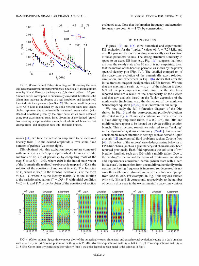
FIG. 3. (Color online) Bifurcation diagram illustrating the vari-ous dark breather/multibreather branches. Specifically, the maximumvelocity of bead 10 versus the frequency fb is shown with a = 0.2 μm.Smooth curves correspond to numerically exact dark breathers; solid(blue) lines indicate the absence of a real instability, and dashed (red)lines indicate their presence (see Sec. V). The linear cutoff frequencyf0 = 7.373 kHz is indicated by the solid vertical black line. Blackcircles represent the experimentally measured mean values (withstandard deviations given by the error bars) which were obtainedusing four experimental runs. Inset: Zoom-in of the dashed (green)box showing a representative example of additional branches thatemerge from (and disappear back into) the main branch.

waves [14], we tune the actuation amplitude to be increasedlinearly from 0 to the desired amplitude a over some fixednumber of periods (we chose eight).

DBs obtained with this excitation procedure are comparedwith numerically exact (up to a prescribed tolerance) periodicsolutions of Eq. (1) of period Tb by computing roots of themap F = u(Tb) − u(0), where u(0) is the initial-state vectorof the (numerically realized) stroboscopic map and u(Tb) is thesolution of the equations of motion at time Tb. The Jacobianof F , which is used in the Newton iterations, is of the formV (Tb) − I , where I is the identity matrix, V is the solutionto the variational equation V ′ = DF · V with initial conditionV (0) = I, and DF is the Jacobian of the equations of motion

evaluated at u. Note that the breather frequency and actuationfrequency are both fb = 1/Tb by construction.

IV. MAIN RESULTS

Figures 1(a) and 1(b) show numerical and experimentalDB excitation for the “typical” values of fb = 7.29 kHz anda = 0.2 μm and the corresponding numerically exact solutionat those parameter values. The strong structural similarity inspace to an exact DB [see, e.g., Fig. 1(a)] suggests that bothare near the steady state after 10 ms. It is not surprising, then,that the motion of the beads is periodic, as shown by the powerspectral density plot [Fig. l(c)]. The detailed comparison ofthe space-time evolution of the numerically exact solution,simulation, and experiment in Fig. 1(b) shows that after theinitial transient stage of the dynamics, a DB is formed. We notethat the maximum strain |un − un+1| of the solution is about60% of the precompression, confirming that the structuresreported here are a result of the nonlinearity of the systemand that any analysis based on the Taylor expansion of thenonlinearity (including, e.g., the derivation of the nonlinearSchrodinger equation [28,29]) is not relevant in our setup.

We now study the full bifurcation diagram of the DBsshown in Fig. 3 and the corresponding profiles/evolutionsillustrated in Fig. 4. Numerical continuation reveals that, fora fixed driving amplitude (here, a = 0.2 μm), the DBs andmultibreathers appear to be located on a single coiling solutionbranch. This structure, sometimes referred to as “snaking”in the dynamical systems community [35–41], has receivedconsiderable recent attention in settings such as nematic liquidcrystals [42] and classical fluid problems such as Couette flow[43]. To the best of the authors’ knowledge, snaking behavior inFPU-like chains (such as a granular crystal chain) has not beenreported previously. Each fold represents the collision of twobreather families, such as a DB with a multibreather. Due tothe “coiling” structure and the nature of excitation simulationsand experiments considered herein (which start with a zeroinitial state), the transition from one multibreather family to thenext as the forcing frequency is increased (or decreased) is notsmooth: saddle-node bifurcations cause the solution to “jump”from lobe to lobe. For example, in Fig. 3 the regions labeled(vii), (v), (iii), and (i) correspond, respectively, to the numberof density dips seen in the (experimental) space-time contour

n

t (m

s)

(a) Exact

5 10 15 200

2

4

6

8

10

n

Simulation

5 10 15 20n

Experiment

5 10 15 20n

t (m

s)

(b) Exact

5 10 15 200

2

4

6

8

10

n

Simulation

5 10 15 20n

Experiment

5 10 15 20n

t (m

s)

(c) Exact

5 10 15 200

2

4

6

8

10

n

Simulation

5 10 15 20n

Experiment

5 10 15 20

FIG. 4. (Color online) Space-time contour plots of the numerically exact, simulated, and experimental evolution leading to a dark breatherwith a = 0.2 μm. (a) Seven-dip solution with fb = 6.35 kHz. (b) Five-dip solution with fb = 6.8 kHz. (c) Three-dip solution with fb =7.15 kHz. Color intensity corresponds to velocity (m/s); the color legend in each panel is the same as in Fig. 1.

032924-3

C. CHONG et al. PHYSICAL REVIEW E 89, 032924 (2014)

n

t (m

s)

(b) (c) a = 0.25 ( μ m)

5 10 15 200

2

4

6

8

10

n

a = 0.37 ( μ m)

5 10 15 20

−0.02

−0.01

0

0.01

0.02

0 0.1 0.2 0.3 0.40

0.005

0.01

v 10 (

m/s

)

a (μ m)

(a) fb = 7.14 (kHz)

(b)

(d)(i)

(iiia)

(iii)

(c)

t (ms)

n

(e) Experiment

0 5 10 15 20 25

5

10

15

20

0

0.2

0.4 (d) Varying amplitude

a (μ

m)

FIG. 5. (Color online) Experimental observation of bistability. (a) Maximum velocity of bead 10 of the exact dark breather versus actuationamplitude a with the frequency fixed as fb = 7.14 kHz. Black points indicate the value a = 0.2 μm, which corresponds to continuationwith respect to the frequency shown in Fig. 3. One can see that the single-dip breather (i) and three-dip breather (iii) are connected by anintermediate unstable solution (iiia). Arrows labeled (b)–(d) describe how the bistability of the system can be realized experimentally [see(b)–(d)]. (b) Experimental space-time contour plots of the velocity. By choosing the actuation amplitude a appropriately one can excite athree-dip breather (a = 0.25 μm). (c) Same as (b), but for an actuation amplitude that dials in a single-dip breather (a = 0.37 μm). Note thatthe three-dip breather terminates at a ≈ 0.36μm in (a). (d) Actuation amplitude profile used to excite a high-energy dark breather. After theinitial linear ramping, the amplitude is kept at a = 0.37 μm for about 10 ms, which will excite a single-dip breather. The single-dip breatheris still maintained even when decreasing the amplitude to a = 0.25 μm. (e) Space-time contour plot corresponding to the actuation amplitudeprofile shown in (d). Color intensity corresponds to velocity (m/s), where the color bar is the same as in (c). Note that if one actuates a restingchain with an actuation amplitude of a = 0.25 μm, then a three-dip breather will emerge [see (b)], thus revealing the system’s bistability.

plot. The label (0) corresponds to the breathers localized nearthe boundaries rather than at the center of the domain. Theexperimentally measured solutions are indicated by filled blackcircles with error bars in Fig. 3.

For example, in region (vii) at fb = 6.35 kHz a solutionwith seven dips emerges from the interference introduced at theboundaries [see Fig. 4(a)]. However, as we gradually increasethe frequency, the outermost dips approach the boundariesuntil the solution collides and vanishes in a saddle-nodebifurcation with an intermediate seven-dip solution, i.e., thesecond lowest branch shown in region (vii) in Fig. 3. As aresult of the disappearance of this branch, the lowest branchin region (v) is made up of solutions with only five dips, e.g.for fb = 6.80 kHz [see Fig. 4(b)]. The cascade of saddle-nodebifurcations continues as we gradually increase the frequency.A solution with only three dips emerges in region (iii), e.g.,for fb = 7.15 kHz [see Fig. 4(c)]. Finally, a single-dip DBemerges for frequencies in region (i), e.g., for fb = 7.29 kHz(see Fig. 1). Thus, we conclude that the actuation frequencythat is chosen will dictate (“dial in”) the number of dips thatwill emerge upon actuation.

A. Experimental observation of bistability

In addition to controlling the multibreather via the fre-quency, one can control the number of dips of the DB byvarying the amplitude. Consider, for example, the three solu-tion branches shown in region (iii) in Fig. 3 at fb = 7.14 kHz.At this frequency the system is bistable, with the three-dipand single-dip breathers being stable and an intermediatethree-dip solution being unstable. These three solutions werecontinued in amplitude [see Fig. 5(a)], revealing a canonicalhysteresis loop between the stable three-dip and the single-dipsolution branches. This enables, even experimentally, a jumpbetween the different solution types [as shown in Fig. 5(b)].One can excite the single-dip breather in the parameter region

a ∈ (0.12,0.37) by first driving to the single-dip breather witha > 0.37 and then adjusting the amplitude to some value in theregion a ∈ (0.12,0.37) [see Fig. 5(d) and 5(e), for example].Note that exciting a resting chain for a fixed frequency in thatregion will yield the three-dip breather [see, e.g., Fig. 5(b)], afeature indicative of the system’s bistability.

V. LINEAR STABILITY ANALYSIS

To investigate the dynamical stability of the obtainedstates, a Floquet analysis was carried out to compute themultipliers associated with the DBs. The Floquet multipliersfor a solution were obtained by computing the eigenvalues ofthe monodromy matrix [which is V (Tb) upon convergence ofthe Newton scheme]. We focus on instabilities associated withsaddle-node bifurcations and pitchfork bifurcations; therefore,we are chiefly interested in the Floquet multipliers on the(positive) real line. However, there can also be oscillatoryinstabilities, which correspond to complex-conjugate pairs ofFloquet multipliers lying outside of the unit circle. Figure 6shows examples of the Floquet multipliers for three single-dipsolutions. The first two examples, in Figs. 6(a) and 6(b), areunstable, but the third example, in Fig. 6(c), is asymptoticallystable. A plot of the magnitude of the multipliers for fixeda = 0.2 μm and various fb is shown in Fig. 6(d). A compli-cation revealed by the Floquet analysis is that, even thoughasymptotically stable solutions are possible, the damping isweak enough that these solutions may not be realizable in the10-ms window considered experimentally. For example, forfb = 7.29 kHz and a = 0.2 μm there is a DB with Floquetmultipliers in the interval |λ| ∈ [0.974,0.998], and thus it isasymptotically stable. Because these multipliers are so nearthe unit circle, converging to a fixed point by repeatedlyapplying F to some initial condition, which is analogous towhat happens when the experiment is run for multiple periods,requires a large number of iterations or running an experiment

032924-4

DAMPED-DRIVEN GRANULAR CHAINS: AN IDEAL . . . PHYSICAL REVIEW E 89, 032924 (2014)

6.8 6.9 7 7.1 7.2 7.3

0.9

1

1.1

fb (kHz)

|λ|

(d)−1 0 1

−1

0

1

Re λ

Im λ

(a) fb = 6.9 (kHz)

−1 0 1Re λ

(b) fb = 7 (kHz)

−1 0 1Re λ

(c) fb = 7.29 (kHz)

FIG. 6. (Color online) Floquet multipliers of the single-dip darkbreather for a = 0.2 μm. (a) At fb = 6.90 kHz the solution is unstabledue to oscillatory instabilities as well as Floquet multipliers on the realline. (b) Floquet multipliers on the real line have retreated within theunit circle at fb = 7.00 kHz but the oscillatory instabilities remain.(c) Finally, at fb = 7.29 kHz all instabilities have vanished, and thesolution is asymptotically stable. (d) Magnitude of Floquet multipliersfor frequencies (kHz) in the interval fb ∈ (6.75,7.4). A dashed (blue)line at |λ| = 1 is also shown to help identify regions of asymptoticstability.

for an extended period of time. Therefore, due to the 10-mswindow used (experimentally), we are often only able to see theexperiment approach the DB and do not see it fully convergeto the DB. Conversely, there also exist oscillatory instabilitieson the solution branch for some parameter intervals. Althoughthe DB is now unstable, we do not expect an oscillatoryinstability to manifest itself in the 10-ms window if we startwith an initial condition near enough to the unstable DB. Inthat case, we have found that the effects of the oscillatoryinstability are typically not observable in computations untilapproximately t = 300 ms. The reason for this is that themagnitudes of the Floquet multiplier pairs associated withthe oscillatory instabilities are often closer to unity than themagnitudes of the unstable Floquet multipliers on the real line.For this reason we only indicate the instabilities due to Floquetmultipliers on the real line [dashed (red) lines] in Fig. 3, eventhough oscillatory instabilities may also be present. A solid(blue) line is shown otherwise, indicating the absence of a realinstability.

VI. A DEEPER THEORETICAL PROBINGOF THE BIFURCATIONS

The bifurcation diagram in Fig. 3 provides a simple yetpowerful qualitative description of the breather structuresthat can emerge in a monatomic granular chain. However,as the above Floquet analysis suggests, there is a deeperstructural complexity that has important implications forthe interpretation of the experimental findings. In particular,there are apparently few regions where the main branch isasymptotically stable (see, e.g., Fig. 6). This begs the question,“Why do the solutions making up the main branch emerge uponexciting a resting chain?” In this section, we unveil severalsubtleties of the bifurcation structure of this system, hoping

6.617 6.619

0.02128

0.02130

0.02132

0.02134

fb (kHz)

v 10 (

m/s

)

(b)

2 4 6 8 10−0.01

−0.005

0

0.005

0.01

n

v n(0)

( m

/s )

(a)

FIG. 7. (Color online) (a) Velocity profile for three variants of athree-dip breather for a = 0.2 μm and fb = 6.62 kHz, indicated bysquares, circles, and triangles at t = 0. Since the solutions have oddsymmetry with respect to the center bead (n = 11), only the left partof the chain is shown. (b) Tight zoom of Fig. 3, where three distinct(but connected) branches can be seen (which cannot be discerned inthe former figure). The three solutions shown in panel (a) lie on thebranches shown in panel (b).

to at least partially explain the answer to this question. Onesubtlety that is not apparent in Fig. 3 is how dense the coilsare. For example, a “zoomed-in” version of one of the coils,shown in Fig. 7(b), reveals that the branch actually coils severaltimes in tight regions in parameter space. Another finer detailis that the primary branch shown in Fig. 3 generates manysecondary and tertiary branches of solutions. Figure 8 showsa “zoomed-out” version of the primary branch, indicating thatthe coiling structure persists well below the 6-kHz frequencylevel that was studied experimentally. The (cyan) diamonds,(green) squares, and black asterisks indicate the presence of(a) pitchfork, (b) period-doubling, and (c) Neimark-Sackerbifurcation points, respectively. The former two are the pointson the main branch where the secondary branches of periodicsolutions are born, whereas the Neimark-Sacker points suggestthe existence of quasiperiodic solutions. We briefly describescenarios (a)–(c) below.

a. Pitchfork bifurcations off the main branch. Severalsecondary branches are initiated by pitchfork bifurcations,either due to a regular pitchfork bifurcation or as part of a pairin what we call a pitchfork loop. To illustrate the difference,we present an example of each type in Fig. 9. The pitchforkloop, shown in Fig. 9(a), consists of a pair of pitchforkbifurcations that are connected. These pitchfork loops appearto be relatively short-lived; i.e., the pitchfork bifurcation that“opens” the loop is near (in terms of arc length) to the pitchforkbifurcation that “closes” the loop. As a result, although themain branch may have an unstable Floquet multiplier onthe real line, there always appears to be a pair of “nearby”solutions that are qualitatively similar to the main branch, withthe addition of a small component that breaks the symmetrythat solutions have on the main branch. However, the twosecondary solutions that comprise the pitchfork loop appearto be symmetric to each other; the only difference betweenthe branches is the direction in which the symmetry-breakingcomponent manifests itself. An example of this is shown inFig. 10. The velocity profile, which is an odd function on themain branch if the center bead is taken as the origin, loses thissymmetry on either branch of the pitchfork loop. This shouldbe contrasted with the “tightly coiled” solutions in Fig. 7,which are perturbations of one another but still have velocity

032924-5

C. CHONG et al. PHYSICAL REVIEW E 89, 032924 (2014)

3.5 4 4.5 5 5.5 6 6.5 7 7.50

0.01

0.02

0.03

0.04

0.05

0.06

0.07

0.08

0.09

0.1

(0)(i)(iii)(v)(vii)

fb (kHz)

v 10 (

m/s

)

FIG. 8. (Color online) An extended illustration of the branch of solutions shown in Fig. 3. As in Fig. 3, the solid (blue) curves indicatethat the real Floquet multipliers are within (or on) the unit circle. A dashed (red) line is shown otherwise. Symbols indicate the presence of abifurcation: black asterisks are Neimark-Sacker bifurcations to T 2 tori, (green) squares are period-doubling bifurcations, and (cyan) diamondsare pitchfork bifurcations. Here, we have plotted only half the total number of torus bifurcations, to avoid obscuring the plot. Dashed linesindicate regions where the N -dip solutions appear as shown in Fig. 3.

profiles that are odd functions, again using the center bead asthe origin. There are also regular pitchfork bifurcations thatproduce solution branches that do not quickly “close.” Werefer to the secondary branches created by these bifurcationsas pitchfork branches and show an example of one in Fig. 9(b).Both types of pitchfork bifurcations stemming from the mainbranch that we studied were unstable for most of the values offb and v10 that were studied experimentally.

b. Period-doubling bifurcations off the main branch. Period-doubling bifurcations are another source of asymmetric peri-odic orbits. As indicated in Fig. 8 by the (green) squares, thereis a number of secondary period 2 branches created by the mainbranch of DBs (which are period 1). In each of the exampleswe found, the eigenvector with λ = −1 is an even function,which breaks the odd symmetry that is present on the mainbranch of solutions. A prototypical example of a secondary,

6.7 6.8 6.9 7 7.1 7.20.005

0.01

0.015

0.02

0.025

0.03

0.035

fb (kHz)

v 10 (

m/s

)

(a)

6.6 6.8 7 7.20

0.01

0.02

0.03

0.04

0.05

fb (kHz)

(b)

FIG. 9. (Color online) Examples of secondary branches with torus bifurcations indicated by black asterisks and pitchfork bifurcationsindicated by (cyan) diamonds. As in Fig. 3, solid (blue) curves indicate that the real Floquet multipliers are within (or on) the unit circle. Adashed (red) line is shown otherwise. The main solution branch is shown in black. (a) Plot of two loops, each of which consists of two pitchforkbifurcations. (b) Plot of pitchfork branches that are not part of a pitchfork loop.

032924-6

DAMPED-DRIVEN GRANULAR CHAINS: AN IDEAL . . . PHYSICAL REVIEW E 89, 032924 (2014)

5 10 15 20−0.02

−0.01

0

0.01

0.02

n

v n(0)

(m/s

)

(a)

8 10 12 14

−0.01

−0.005

0

0.005

0.01

n

(b)

FIG. 10. (Color online) (a) Plot of the velocity profiles at t = 0 oneither “arm” of the pitchfork loop shown in the inset in Fig. 3, whichdemonstrate the symmetry breaking that occurs when the forcingamplitude is at a maximum. The solid (blue) line is the lower branch,while the dashed (green) line is the upper branch. (b) Zoom-in of (a)around beads 8–14.

period 2 branch is shown in Fig. 11. This period 2 branch actsas a “bridge” between two sides of a single “lobe” of period 1solutions as indicated by the pair of pitchfork bifurcationsat the start and end of the period 2 branch of solutions(each bifurcation is indeed a pitchfork, but the ordinate inFig. 11, which is the maximum velocity of the tenth bead,causes two branches of the pitchfork to appear practicallyidentical). As in the period 1 branch, the period 2 branchcontains its own set of bifurcations including additional branchpoints, period-doubling bifurcations, and Neimark-Sackerbifurcations, each of which could create tertiary period 2,period 4, and quasiperiodic solutions, respectively. However,none of the tertiary period 2 or period 4 branches we examinedwas born stable at their associated bifurcation points, norwas stability regained in the tertiary branch. Although oursearch of these regions is less than exhaustive, the (quitecommon) tertiary branches stemming from period 2 brancheswe computed were unstable.

c. Quasiperiodic solutions. Within the framework of classi-cal dynamical systems theory, one would expect quasiperiodic

FIG. 11. (Color online) (a) Example of a period 2 branch ofsolutions is shown in blue and red; solid (blue) curves indicate thatthe real Floquet multipliers are within (or on) the unit circle. A dashed(red) line is shown otherwise. The black curve denotes the period 1branch of solutions, and the markers indicate pitchfork bifurcation[(cyan) diamonds], period-doubling bifurcations [(green) squares],and Neimark-Sacker bifurcations (black asterisks). (b) A zoom-in of(a) showing how each end of the period 2 branch is connected to themain branch by a pair of pitchfork bifurcations.

solutions to exist in the system given the presence of Neimark-Sacker points. A quasiperiodic solution is a continuous timetrajectory on a torus in phase space; in the stroboscopicmap, that same quasiperiodic solution appears as an invariantcircle. Analogous to the periodic orbits generated by Hopfbifurcations, Neimark-Sacker bifurcations produce invariantcircles that can be either stable or unstable. While algorithmsfor approximating invariant circles exist [44], continuingbranches of quasiperiodic orbits via Newton’s method liesoutside the scope of this paper. However, in the neighborhoodof a supercritical Neimark-Sacker bifurcation, it is possible toapproximate the invariant circle by iterating the stroboscopicmap a large number of times as demonstrated in Fig. 12.Clearly, such an approach is only feasible when the invariantcircle (or, in a flow, the torus) is asymptotically stable, asthe rate of convergence is dependent upon the “least stable”eigenvalue. As such, Fig. 12 shows two examples on the same“branch” of solutions obtained by computing 105 successiveiterates of the stroboscopic map for each new value of fb andthen plotting the next 5000–10 000 iterates of the stroboscopicmap, with one marker every 10 iterates. At fb = 7.487 kHz,we have identified what appears to be a quasiperiodic orbitas shown in Figs. 12(a) and 12(b). Figure 12(a) shows thedisplacement and velocity of the tenth bead at the start ofevery forcing period. Smaller (blue) dots denote the state ofthe system (in this projection) after every 10 iterates of thestroboscopic map, while filled (green) circles denote the last20 iterates of the map; finally, the filled (red) circle in the centeris the period 1 solution at this frequency. Although the presenceof an invariant circle is clear in this projection, it should benoted that it requires several thousand iterations to reach thevicinity of the invariant circle given an initial condition thatis a small perturbation of the period 1 solution. This is due tothe fact that we are near the Neimark-Sacker bifurcation point,so the unstable pair of eigenvalues is only slightly larger thanunity in magnitude. However, the invariant circle itself appearsto be stable even in the face of large perturbations. Figure 12(b)shows the relative distance between two nearby trajectoriesas a function of the iterations of the stroboscopic map. Toproduce this plot each (nondimensionalized) component of apoint on the invariant circle was perturbed with a small “kick”drawn from a normal distribution with a standard deviation of10−5, which is small compared to typical, nondimensionalizeddisplacement and velocities at this forcing frequency. Themain result is that points that are not too far apart willconverge as the perturbed solution is attracted back to theinvariant circle and will remain close for all future times. Thisbehavior should be contrasted with what occurs at fb = 7.462kHz, which is shown in Figs. 12(c) and 12(d). Althoughthe dynamics shown in Fig. 12(c) appear to lie on a higherdimensional torus, say, a T 3 torus, the plot of the distancebetween nearby initial conditions in Fig. 12(d) indicates thatwe are more likely on a chaotic attractor, as nearby trajectoriesdiverge after sufficiently long periods of time. This can beexplained by the Ruelle-Takens-Newhouse route to chaos,which is based on the observation that a constant vectorfield on a T 3 torus can be perturbed by an arbitrarily smallamount to produce a chaotic attractor [45]. As a result, thequasiperiodic solution at fb = 7.487 kHz likely underwentanother transition at some higher frequency, which results

032924-7

C. CHONG et al. PHYSICAL REVIEW E 89, 032924 (2014)

×× ××

FIG. 12. (Color online) (a) Demonstration of the invariant circle created by plotting several thousand iterates of the map F with fb =7.487 kHz; smaller (blue) dots indicate the velocity of the tenth bead recorded every 10/fb s, filled (green) circles denote the last 20 iterates ofthe map, and the filled (red) circle in the center denotes the unstable period 1 orbit. (b) The log of the normalized distance between two nearbyinitial conditions as a function of time; though the exact distance is time dependent, trajectories on the invariant circle that start near eachother remain near each other. (c) Demonstration of the stroboscopic map with fb = 7.462 colored as in the leftmost plot; if more iterationsare plotted, the trajectory will eventually “fill in” the region. (d) Pairs of nearby trajectories will separate after a sufficiently large number ofiterations, which suggests the presence of a chaotic attractor.

in the observed dynamics at 7.462 kHz. We should pointout that not all of the Neimark-Sacker bifurcations in Fig. 8result in stable quasiperiodic orbits. In principle, subcriticalNeimark-Sacker bifurcations will produce unstable invariantcircles that cannot be continued using the straightforwardcomputational procedure used to produce Fig. 12 but couldbe continued using more sophisticated techniques like thosein Ref. [44].

A. Implication of secondary structures for experiments

Due to the number of bifurcations that generate secondarybranches and the complexity and additional bifurcations thatappear on those branches, this system apparently gives riseto a veritable “zoo” of dynamics and displays a vast array ofdifferent nonlinear behaviors. To complicate matters further,there are also additional branches of periodic solutions withlonger periods (e.g., period 2 solutions of the map F thathave period 2Tb) whose shapes and bifurcations are alsonontrivial. Both these larger period solutions and solutionson the pitchfork branches generate tertiary branches, which,in principle, could be asymptotically stable in the region ofexperimental interest but, in our experience, are typicallyunstable. As shown in Fig. 8 and Fig. 9, the main branchand the secondary branches are filled with Neimark-Sackerbifurcations. This gives many opportunities for the creation ofquasiperiodic solution branches, where the dynamics lies onan invariant circle in the stroboscopic map (and a torus in theflow). Thus, it is possible that some of the solutions observedexperimentally actually lie on or near a slowly modulated torus(which live near the main branch of period 1 DBs). However,observing the true quasiperiodic nature of these solutionsexperimentally may be difficult; in the numerical studyperformed here, thousands of forcing periods were requiredbefore the quasiperiodic structure of the solution became clear.Our answer to the question posed at the beginning of thissection is as follows: There is a very rich variety of periodicsolutions that exist. There are additional nearby invariantobjects (tori, chaotic solutions) and long transients associated

with global bifurcations that also “lurk” in the neighborhood ofthese solutions. Thus, a trajectory starting from zero initial datais highly nontrivial and appears to be influenced by the zoo ofstructures that exist in parameter space. Indeed, one is often notcompletely certain that a “visually close to periodic” transienthas actually converged to a limit cycle on a particular branch.Ultimately, our comparison of theory and experiment suggeststhat it is possible to obtain a good qualitative description of theobserved dynamics based on the main branch of period 1 solu-tions. This was true even in unstable regions, probably due tothe existence of similar structures that live near the main branchof period 1 solutions, which, given our investigations, areplentiful.

VII. CONCLUSIONS AND FUTURE CHALLENGES

The damped-driven granular crystal system has been shownto provide access to a rich family of DB and multibreathersolutions. In fact, it can be argued that the resulting mappingof the system’s solutions appears to be far richer than what hasbeen previously explored for any breather structure in granularchains (and, in the context of DBs, for any physical system).The system possesses an intricate bifurcation diagram wherethe stable single- and multidip solutions are interlaced viaunstable intermediate branches (i.e., snaking behavior). The di-agram contains a large number of saddle-node bifurcations andassociated fold points, as well as pitchfork symmetry-breakingpoints. This structure provides not only hysteresis loops andmultistability regimes, but also a remarkable tunability andnumerous branches of more complex period 2, quasiperiodic,and even chaotic attractor solutions. We have offered, throughour dynamical systems analysis, a roadmap towards theidentification of these solutions, although some of them(especially the more complex ones, including quasiperiodicand chaotic solutions) clearly merit further investigation.The selection of driving frequency and amplitude enables aselection of multibreather configurations robustly sustainedby the dynamics. The coherent structures produced herein

032924-8

DAMPED-DRIVEN GRANULAR CHAINS: AN IDEAL . . . PHYSICAL REVIEW E 89, 032924 (2014)

0 0.02 0.04 0.06

−5

0

5

V [m

m/s

]

0 0.02 0.04 0.06

−25

−20

−15

log(

E)

Time [s]

(b)

(d)

0 0.02 0.04 0.06

−5

0

5

V [m

m/s

]

0 0.02 0.04 0.06

−25

−20

−15

Time [s]

log(

E)

(a)

(c)

(e)

4000 5000 6000 7000 8000

−100

−50

0

Frequency [Hz]

Tra

nsm

issi

on [d

B]

ExperimentSimulation

FIG. 13. (Color online) Temporal profiles of the 21st particle’s velocity and kinetic energy. (a, c) Experimental measurements.(b, d) Numerical simulations. (e) Experimental (red line) and numerical (blue line) results of transmission gains of the granular chain.

could be utilized towards controllable energy funneling andharvesting within granular media.

ACKNOWLEDGMENTS

The authors would like to thank G. Theocharis foruseful discussions. Support from the US NSF (Grant Nos.CMMI 1310173, CMMI 1234452, and CMMI 1000337) andUS AFOSR (Grant No. FA9550-12-1-0332) is appreciated.M.O.W. gratefully acknowledges support from an NSF Math-ematics Sciences Postdoctoral Research Fellowship, DMS1204783.

APPENDIX: DAMPING COEFFICIENT DETERMINATION

The damping mechanism in the granular system is modeledby the simple mathematical term M

τun, as expressed in Eq. (1).

Despite its simplicity, this dash-pot model has proven tobe effective in granular systems as reported in previousstudies, including the authors’ recent work [22,27]. Thedamping coefficient τ is determined empirically to reflectthe degree of dissipation in the given experimental system.More specifically, we excite the chain with harmonic pulses,with a = 0.03 μm and f = 4.815 kHz, and then quench theexcitation at ≈28 ms. The temporal velocity profile of the

21st particle (i.e., the last particle in the chain) is shown inFig. 13(a) based on the measurements with a laser Dopplervibrometer. Based on this velocity profile, Fig. 13(c) plotsthe decay of the kinetic energy in logarithmic scale. Weobserve that the slope of the kinetic energy decay is linearafter 28 ms. This, in turn, leads to the empirical value ofτ ≈ 5 ms based on the fitting of this decaying slope [blueline in Fig. 13(c)]. We validate this value by reproducingthe decaying curves numerically [Figs. 13(b) and 13(d)].The simulation results are in excellent agreement with theexperimental results. Since the aforementioned damping factorwas determined at a single excitation frequency, we need tocheck the efficacy of this damping model over a broad rangeof the frequency domain. First, we obtain the experimentalbaseline of the system’s frequency response by measuring itstransmission gain in terms of the power spectral density usinga network analyzer (Agilent 4395A). Then we calculate itsnumerical counterpart by solving the differential equation ofthe system [Eq. (1)] using the empirically obtained dampingparameter. The experimental and numerical results are plottedin Fig. 13(e) by the red and blue curves, respectively. Thenumerical results successfully capture the dynamic responseof the system over the broad range of the pass band, confirmingthe validity of our simple damping model.

[1] S. Flach and A. V. Gorbach, Phys. Rep. 467, 1 (2008).[2] F. Lederer, G. I. Stegeman, D. N. Christodoulides, G. Assanto,

M. Segev, and Y. Silberberg, Phys. Rep. 463, 1 (2008).[3] M. Sato, B. E. Hubbard, and A. J. Sievers, Rev. Mod. Phys. 78,

137 (2006).[4] P. Binder, D. Abraimov, A. V. Ustinov, S. Flach, and

Y. Zolotaryuk, Phys. Rev. Lett. 84, 745 (2000); E. Trıas, J. J.Mazo, and T. P. Orlando, ibid. 84, 741 (2000).

[5] L. Q. English, M. Sato, and A. J. Sievers, Phys. Rev. B 67,024403 (2003); U. T. Schwarz, L. Q. English, and A. J. Sievers,Phys. Rev. Lett. 83, 223 (1999).

[6] B. I. Swanson, J. A. Brozik, S. P. Love, G. F. Strouse, A. P.Shreve, A. R. Bishop, W.-Z. Wang, and M. I. Salkola, Phys.Rev. Lett. 82, 3288 (1999).

[7] M. Peyrard, Nonlinearity 17, R1 (2004).[8] O. Morsch and M. Oberthaler, Rev. Mod. Phys. 78, 179

(2006).

[9] A. Chabchoub, O. Kimmoun, H. Branger, N. Hoffmann,D. Proment, M. Onorato, and N. Akhmediev, Phys. Rev. Lett.110, 124101 (2013).

[10] A. Weller, J. P. Ronzheimer, C. Gross, J. Esteve, M. K.Oberthaler, D. J. Frantzeskakis, G. Theocharis, and P. G.Kevrekidis, Phys. Rev. Lett. 101, 130401 (2008); S. Stellmer,C. Becker, P. Soltan-Panahi, E.-M. Richter, S. Dorscher,M. Baumert, J. Kronjager, K. Bongs, and K. Sengstock, ibid.101, 120406 (2008).

[11] D. J. Frantzeskakis, J. Phys. A 43, 213001 (2010).[12] W. Tong, M. Wu, L. D. Carr, and B. A. Kalinikos, Phys. Rev.

Lett. 104, 037207 (2010).[13] A. Kanshu, C. Ruter, D. Kip, J. Cuevas, and

P. G. Kevrekidis, Eur. Phys. J. D 66, 182(2012).

[14] V. F. Nesterenko, Dynamics of Heterogeneous Materials(Springer-Verlag, New York, 2001).

032924-9

C. CHONG et al. PHYSICAL REVIEW E 89, 032924 (2014)

[15] S. Sen, J. Hong, J. Bang, E. Avalos, and R. Doney, Phys. Rep.462, 21 (2008).

[16] C. Daraio, V. F. Nesterenko, E. B. Herbold, and S. Jin, Phys.Rev. Lett. 96, 058002 (2006).

[17] J. Hong, Phys. Rev. Lett. 94, 108001 (2005).[18] F. Fraternali, M. A. Porter, and C. Daraio, Mech. Adv. Mat.

Struct. 17(1), 1 (2010).[19] R. Doney and S. Sen, Phys. Rev. Lett. 97, 155502 (2006).[20] D. Khatri, C. Daraio, and P. Rizzo, SPIE 6934, 69340U (2008).[21] A. Spadoni and C. Daraio, Proc. Natl. Acad. Sci. USA 107, 7230

(2010).[22] N. Boechler, G. Theocharis, and C. Daraio, Nature Mater. 10,

665 (2011).[23] C. Daraio, V. F. Nesterenko, E. B. Herbold, and S. Jin, Phys.

Rev. E 72, 016603 (2005).[24] V. F. Nesterenko, C. Daraio, E. B. Herbold, and S. Jin, Phys.

Rev. Lett. 95, 158702 (2005).[25] G. Theocharis, M. Kavousanakis, P. G. Kevrekidis, C. Daraio, M.

A. Porter, and I. G. Kevrekidis, Phys. Rev. E 80, 066601 (2009);S. Job, F. Santibanez, F. Tapia, and F. Melo, ibid. 80, 025602(2009); Y. Man, N. Boechler, G. Theocharis, P. G. Kevrekidis,and C. Daraio, ibid. 85, 037601 (2012).

[26] N. Boechler, G. Theocharis, S. Job, P. G. Kevrekidis, M. A.Porter, and C. Daraio, Phys. Rev. Lett. 104, 244302 (2010);G. Theocharis, N. Boechler, P. G. Kevrekidis, S. Job, M. A.Porter, and C. Daraio, Phys. Rev. E 82, 056604 (2010).

[27] C. Hoogeboom, Y. Man, N. Boechler, G. Theocharis, P. G.Kevrekidis, I. G. Kevrekidis, and C. Daraio, Eur. Phys. Lett.101, 44003 (2013).

[28] C. Chong, P. G. Kevrekidis, G. Theocharis, and C. Daraio, Phys.Rev. E. 87, 042202 (2013).

[29] G. Schneider, Appl. Anal. 89, 1523 (2010).[30] A. Alvarez, J. F. R. Archilla, J. Cuevas, and F. R. Romero, New

J. Phys. 4, 72 (2002).[31] G. James, J. Nonlin. Sci. 13, 27 (2003).[32] B. Sanchez-Rey, G. James, J. Cuevas, and J. F. R. Archilla, Phys.

Rev. B 70, 014301 (2004).[33] http://www.efunda.com.[34] F. Li, L. Yu, and J. Yang, J. Phys. D: Appl. Phys. 46, 155106

(2013).[35] J. Burke and E. Knobloch, Chaos 17, 037102 (2007).[36] J. H. P. Dawes, SIAM J. Appl. Dyn. Syst. 7, 186 (2008).[37] S. G. McCalla and B. Sandstede, Physica D 239, 1581 (2010).[38] A. Bergeon, J. Burke, E. Knobloch, and I. Mercader, Phys. Rev.

E 78, 046201 (2008).[39] J. Knobloch, D. J. B. Lloyd, B. Sandstede, and T. Wagenknecht,

J. Dyn. Diff. Eqs. 23, 93 (2011).[40] M. Beck, J. Knobloch, D. J. B. Lloyd, and B. T. Sandstede

Wagenknecht, SIAM J. Math. Anal. 41, 936 (2009).[41] C. Taylor and J. H. P. Dawes, Phys. Lett. A 375, 14 (2010).[42] F. Haudin, R. G. Rojas, U. Bortolozzo, S. Residori, and M. G.

Clerc, Phys. Rev. Lett. 107, 264101 (2011).[43] T. M. Schneider, J. F. Gibson, and J. Burke, Phys. Rev. Lett.

104, 104501 (2010).[44] I. G. Kevrekidis, R. Aris, L. D. Schmidt, and S. Pelikan, Physica

D 16, 243 (1985).[45] S. E. Newhouse, D. Ruelle, and F. Takens, Commun. Math.

Phys. 64, 35 (1978).

032924-10