d3.2.1 models and simulators report - cordis · doc ref: deliverable 3.2.1 ... land use model which...

Public

© All Rights Reserved

Consensus Deliverable 3.2.1 Page i of viii

The research leading to these results has received funding from the European Community's Seventh Framework Programme [FP7/2007-2013] under grant agreement no. 611688

SEVENTH FRAMEWORK PROGRAMME

THEME ICT-2013.5.4

"ICT for Governance and Policy Modelling"

D3.2.1

Models and Simulators Report

Project acronym: Consensus

Project full title: Multi-Objective Decision Making Tools through Citizen Engagement

Contract no.: 611688

Workpackage: WP3 Models and Simulators

Editor: Stefan Frank IIASA

Author(s): Stefan Frank, Petr Havlik, Michael

Obersteiner

IIASA

Angeliki Kopsacheili, George Yannis,

Konstantinos Diamandouros

ERF

Vaggelis Psomakelis, Konstantinos Tserpes NTUA

Authorized by Konstantinos Tserpes NTUA

Doc Ref: Deliverable 3.2.1

Reviewers Giorgia Ceccarelli, Frederica Corsi OXFAM

Dissemination Level Public

Public


Consensus Deliverable 3.2.1 Page ii of viii


Consensus Consortium

No Name Short name Country

1 Institute of Communication and Computer

Systems/National Technical University of Athens

NTUA Greece

2 IBM Israel Science and Technology Ltd. IBM Israel

3 International Institute for Applied Systems Analysis IIASA Austria

4 Athens Technology Center ATC Greece

5 University of Konstanz UKON Germany

6 OXFAM Italia ONLUS OXFAM Italy

7 WWF - World Wide Fund for Nature WWF Switzerland

8 European Union Road Federation ERF Belgium

Document History

Version Date Changes Author/Affiliation

v.0.1 25-06-2014 TOC S. Frank/IIASA

v.0.2 04-07-2014 TOC Review K. Tserpes/NTUA

v.0.3 23-07-2014 TOC update A. Kopsacheili/ERF

V. Psomakelis/NTUA

S. Frank/IIASA

v. 0.4 29-08-2014 Draft version All contributors

v. 0.5 15-09-2014 Revision by all contributors and

reviewers

All contributors and

reviewers

v. 1.0 30-09-2014 Final version S. Frank/IIASA

Public


Consensus Deliverable 3.2.1 Page iii of viii


Executive Summary Deliverable D3.2.1 “Models and Simulators report” presents the first report on the models

and simulators used and developed in Consensus. It is designed to give an overview and an in

depth guide for the installation and application of the model prototypes.

According to the Consensus “Description of Work”, this deliverable is public. It is submitted in

month 12 as part of the work associated to the WP3, “Models and Simulators”. This report

represents the first deliverable in a series of three. It will be updated in month 24 and month

30.

This document is organised in four Chapters.

Chapter 1 provides an introduction explaining the purpose and the objectives of this

document.

Chapter 2 includes a detailed description of the GLOBIOM model. GLOBIOM is an economic

land use model which will be used to quantify the impact of European biofuel policies on

sustainability objectives. In this section, the model will be presented briefly, followed by a

description of the biofuel policy scenarios and sustainability criteria reported. At the end of

the chapter, guidelines for the installation and use of the prototype delivered in D3.1.1 can

be found.

Chapter 3 present the Road Transport model which will be applied in the road pricing policy

context. First the development and structure of the model will be presented followed by a

description of the road transportation scenarios and a guide for installation and use of the

prototype.

Chapter 4 presents the Public Acceptability model which will allow quantifying the public

acceptability of the different biofuel and road transportation policies. The section includes a

model description followed by a prototype installation and application guide.

Public


Consensus Deliverable 3.2.1 Page iv of viii


Table of Contents Executive Summary ................................................................................................................... 3

Table of Contents ...................................................................................................................... 4

List of Tables .............................................................................................................................. 7

Referenced project deliverables ............................................................................................... 7

1 Introduction ....................................................................................................................... 1

1.1 Scope and objectives................................................................................................ 1

1.2 Structure .................................................................................................................. 1

2 An enhanced model for multi-criteria assessment of EU bioenergy policies – GLOBIOM 2

2.1 Introduction ............................................................................................................. 2

2.2 GLOBIOM – model description ................................................................................ 3

2.2.1 Model Structure and datasets ........................................................................... 3

2.2.2 Important GLOBIOM features ........................................................................... 5

2.2.3 Model outputs ................................................................................................... 8

2.3 Biofuel policy scenarios .......................................................................................... 11

2.4 Prototype application ............................................................................................ 16

2.4.1 Installation ....................................................................................................... 16

2.4.2 Usage ............................................................................................................... 17

3 Transport modeling framework ...................................................................................... 18

3.1 Introduction ........................................................................................................... 18

3.2 State-of-the-Art review .......................................................................................... 18

3.2.1 Modelling techniques in transport sector ....................................................... 18

3.2.2 Modelling practices for estimating the impacts of road pricing ..................... 19

3.2.3 Modelling assumptions and data requirements in road pricing analyses....... 20

3.3 Modelling framework for the Consensus transport policy scenario – prototype

description and application ................................................................................................. 20

Public


Consensus Deliverable 3.2.1 Page v of viii


3.3.2 Perceptual stage .............................................................................................. 26

3.3.3 Conceptual stage ............................................................................................. 30

3.3.4 Computing stage .............................................................................................. 45

3.3.5 Calibration and validation stages .................................................................... 53

4 A modelling mechanism for the policy implementation acceptability ........................... 55

4.1 Introduction ........................................................................................................... 55

4.1.1 Scientific background ...................................................................................... 56

4.2 Model description .................................................................................................. 57

4.2.1 Experiments and results .................................................................................. 57

4.2.2 Component architecture ................................................................................. 58

4.2.3 Future plans ..................................................................................................... 59

4.3 Prototype application ............................................................................................ 60

4.3.1 Requirements .................................................................................................. 60

4.3.2 Installation and deployment ........................................................................... 60

4.3.3 Usage ............................................................................................................... 60

5 References ....................................................................................................................... 64

Public


Consensus Deliverable 3.2.1 Page vi of viii


List of Figures

Figure 1: GLOBIOM in the Consensus Framework .................................................................... 2

Figure 2. GLOBIOM model structure ......................................................................................... 3

Figure 3. GHG emission sources in GLOBIOM ........................................................................... 6

Figure 4. Biofuel Sustainability pillars ....................................................................................... 9

Figure 5. Options menu in GAMS. ........................................................................................... 17

Figure 6. Road Pricing Model Role and Structure ................................................................... 25

Figure 7. Model Development Stages ..................................................................................... 26

Figure 8. Impacts of road pricing on travel and transportation costs (Source: CEDR, 2009) .. 26

Figure 9. Impacts of road pricing on road network functionality (Source: CEDR, 2009) ........ 27

Figure 10. Impacts of road pricing on traffic safety (Source: CEDR, 2009) ............................. 28

Figure 11. Impacts of road pricing on the environment (Source: CEDR, 2009) ...................... 28

Figure 12. Impacts of road pricing on travel convenience (Source: CEDR, 2009) ................... 29

Figure 13. Impacts of road pricing on road funding (Source: CEDR, 2009) ............................. 29

Figure 14. Schematic of basic PDFH-style forecast (Source: Arup & Oxera, 2010) ................. 35

Figure 15. Acceptability model architecture. .......................................................................... 59

Public


Consensus Deliverable 3.2.1 Page vii of viii


List of Tables Table 1. Main GLOBIOM characteristics .................................................................................... 4

Table 2. Biofuel policy scenario sustainability criteria. ............................................................. 9

Table 3: Reference scenario drivers. ....................................................................................... 11

Table 4. Scenario set-up for the biofuel policy scenarios quantified in phase 1 of Consensus.

................................................................................................................................................. 13

Table 5. Alternative Scenarios Components (road pricing policy schemes including road

project development options and details) .............................................................................. 21

Table 6. Objectives and their metrics for road pricing schemes evaluation ........................... 22

Table 7. Car Values of Time, for different trip purposes, in European countries

(€/passenger/hour, in 2012 prices) ......................................................................................... 32

Table 8. Comparison of truck and car Values of Time ............................................................. 33

Table 9. Unit values for accidents in European countries (in €ct/vkm) – for main network

types and vehicle categories ................................................................................................... 38

Table 10. Unit values for air pollution costs (EU-27), (in €ct/vkm) - for main network types

and vehicle categories ............................................................................................................. 40

Table 11. Unit values for noise costs (EU-27), (in €ct/vkm) - for main network types and

vehicle categories .................................................................................................................... 41

Table 12. “Relative Investment Cost” Objective Estimation ................................................... 42

Table 13. Relative Operational Cost, as a % of gross revenues, for different Toll Collection

Techniques and other (decisive) components of a road pricing scheme ................................ 44

Table 14 “User Convenience” Objective Estimation ............................................................... 45

Table 15. “Ensure Social Fairness” Objective Estimation ........................................................ 45

Table 16. HCM Level of Service Criteria, for basic freeway sections....................................... 51

Table 17. Model calibration criteria ........................................................................................ 53

Table 18. Available algorithms and keywords. ........................................................................ 61

Referenced project deliverables D2.1.1: User requirements, ERF, Consensus Project Report, Confidential, available only to

project members and review panel

Public


Consensus Deliverable 3.2.1 Page viii of viii


D4.1.1: Optimization and Visual analytics Prototypes, IBM, Consensus Project Prototypes,

Confidential, available only to project members and review panel

D2.2: State of the art report, ERF, Consensus Project Report, Public, available at:

http://consensus-project.eu

D2.3: Domain Data Sources, ICCS/NTUA, Confidential, available only to project members and

review panel

D3.2.1: Models and Simulators Report, IIASA, Consensus Project Report, Public, available at

http://www.consensus-project.eu/deliverables

D2.4.1: System Architecture, NTUA, Consensus Project Report, Confidential, available only to

project members and review panel

Public


Consensus Deliverable 3.2.1 Page 1 of 71

1 Introduction The Consensus project aims to assist policy makers to decide upon different policies taking

into account not only the effectiveness with respect to one particular policy objective but

also potential trade-offs with other objectives. In this framework, Consensus aims to deliver

the two following stand-alone tools:

- The ConsensusMOOViz: A web interface intended for the policy maker (or someone

close to the policy maker) that will in an easy and comprehensive manner analyse and

visualise the consequences of policy decisions, and further provide policy makers with

structured approach for exploring and selecting optimal choices based on a number of

relevant criteria.

- The ConsensusGames: A web interface intended for the general public to educate

citizens regarding the consequences of certain policy implementation options and for

harvesting user preferences to include public opinion in the policy making process.

1.1 Scope and objectives The main scope of deliverable “D3.2.1 Models and Simulators Report” is to provide a

detailed overview of the models developed and applied in the first year of Consensus. This

deliverable includes an extensive documentation of the models, model developments and

research conducted. In addition, the deliverable provides an installation and application

guideline for the different prototypes delivered in “D3.1.1 Models and Simulators

Prototypes” as well as a description of the biofuel and road pricing policy scenarios.

The main objectives of D3.2.1 can be summarized as following according to the “Description

of Work” document:

Provide a description of the models and components developed based on the

research conducted.

Provide a set of model scenarios for multi-objective solvers (biofuel and road

transportation case studies).

Provide a guide for installation, deployment and use of the prototypes delivered.

1.2 Structure

1 This deliverable is organized in 4 chapters. After the current chapter the three models

(land use-, road transportation- and public acceptability model) are presented in each

subsequent chapter. Chapter 2 provides a description of IIASA’s GLOBIOM model and

the biofuel policy scenarios. Chapter 3 includes a description of ERF’s Road

Transportation Model and the road transportation scenarios. Finally, in chapter 4

NTUA’s Public Acceptability Model is presented. Each chapter includes a detailed model

description followed by a description of the scenarios where relevant and a guide for

installation and application of the prototype.

Public



2 An enhanced model for multi-criteria assessment of EU

bioenergy policies – GLOBIOM

2.1 Introduction The Global Biosphere Management Model (GLOBIOM) is a global economic land use model.

It has been developed at the International Institute for Applied Systems Analysis (IIASA)

since 2007. The GLOBIOM model is mainly applied around WP3 “Models and Simulators”. It

is used to quantify various biofuel policy scenarios and assess the impact of biofuels on

different sustainability pillars (environment, climate change mitigation, food security and

economy). Model outputs feed into various other Consensus components such as the Multi-

Objective Solvers, Visualization and Gaming Tools in WP4. For each of biofuel scenario (see

chapter “2.3 Biofuel policy scenarios”) sustainability criteria for different sustainability pillars

are communicated to the Multi-Objective Solvers and consequently the Visualization and

Gaming tools. The sustainability criteria reported by GLOBIOM serve as a “scenario surface”

for the Multi-Criteria Optimization. Figure 1 illustrates the position of GLOBIOM within the

Biofuel Policy assessment, in Consensus.

Figure 1: GLOBIOM in the Consensus Framework

In month 6, deliverable “D2.1.1 User Requirements” provided a first description of the

GLOBIOM model including a description of the general model structure, the modelling

approach as well as the underlying datasets. A technical description which listed key

variables, equations and model outputs has been delivered in “D2.4.1 System Architecture”.

A description of the optimization in GLOBIOM can be found in “D4.2.1 Optimization and

Visual Analytics Reports”.

In order to avoid repetition, we present here only briefly the general model structure,

datasets used as well as output criteria reported. Instead, we focus in this deliverable on

model characteristics, which are of special interest for the Consensus project, namely

important characteristics for a consistent biofuel assessment. In the second part of this

chapter, we present in detail the biofuel policy scenarios modelled and provide a user

Biofuel Policy

Scenarios

GLOBIOM Multi Criteria

Optimization

Solvers

Visualization

Tools

CONSENSUS

game

Public



guideline which should enable the end-user to successfully apply and understand the

prototype delivered in “D3.1.1 Model and Simulators Prototypes”.

2.2 GLOBIOM – model description

2.2.1 Model Structure and datasets

GLOBIOM is a global economic land use model with the aim to provide policy analysis on

global issues concerning land use competition between the major land-based production

sectors. GLOBIOM is a global recursive dynamic bottom-up partial equilibrium model

integrating the agricultural, bioenergy and forestry sectors. It represents all world regions

aggregated to 57 regions. Partial equilibrium denotes that the model does not include the

whole range of economic sectors in a country or region but represent only the main land

based sectors, namely the agriculture, forestry and bioenergy production. However, these

sectors are modelled in a great detail. Figure 2 presents the model structure graphically

while main model characteristics are presented in Table 1.

Figure 2. GLOBIOM model structure

Public



In the objective function of the model, a global agricultural and forest market equilibrium is

computed by choosing land use and processing activities to maximize welfare (i.e. the sum

of producer and consumer surplus) subject to resource, technological, demand and policy

constraints (see “D2.4.1 System Architecture” for GLOBIOM equations and variables and

“D4.2.1 Optimization and Visual Analytics Reports” for optimization components).

GLOBIOM is calibrated to the year 2000 and run recursively dynamic in 10-year time-steps

up to 2050. In contrast to fully dynamic models which optimize over all time periods

simultaneously, GLOBIOM optimizes only one period at once. However, the solution in a

period is dependent on the solution of the previous periods solved i.e. previous land use

changes are transmitted from one period to the next and alter the land availability in the

different land categories in the next period.

Table 1. Main GLOBIOM characteristics

GLOBIOM

Model framework Bottom-up, starts from land and technology at grid level

Sector coverage Detailed focus on agriculture, forestry and bioenergy (partial equilibrium)

Regional coverage Global (28 EU Member states + 29 regions ROW)

Resolution on production side Detailed grid-cell level

Time frame 2000-2050 (ten year time step)

Market data source EUROSTAT and FAOSTAT

Land use change mechanisms Geographically explicit. Land conversion possibilities allocated on grid-cells taking into account suitability, protected areas.

Representation of technology Detailed biophysical models estimates for agriculture and forestry with several management systems

Demand side representation On representative consumer per region and per good, only reacting to price

GHG accounting 12 sources of GHG emissions covering crop cultivation, livestock, land use change etc.

Demand for final products, prices and international trade are represented at the level of 57

aggregated world regions (28 EU member countries, 29 regions outside Europe). Commodity

demand is specified as downward sloped iso-elastic function parameterized using FAOSTAT

data on prices and quantities, and price elasticities as reported by Muhammad [1].

On the supply side, land resources and their characteristics are the fundamental elements of

our bottom-up modelling approach. Therefore, the model is based on a detailed

disaggregation of land into Simulation Units (SimU) – clusters of 5 arcmin pixels belonging to

the same country, altitude, slope and soil class and to the same 0.5° x 0.5° pixel [2]. SimUs

delineation builds on a comprehensive global database, which contains geo-spatial data on

soil, climate/weather, topography, land cover/use, and crop management (e.g. fertilization,

Public



irrigation). Cropland, grassland, forest and short rotation tree plantation productivity is

computed together with related environmental parameters like greenhouse gas (GHG)

budgets or fertilizer and water requirements at the SimU level, either by means of process

based biophysical models or by means of downscaling from national data sets. Production

technologies at the level of SimU, or their aggregates, are specified through Leontief

production functions, which imply fixed input – output ratios.

On the crop production side, GLOBIOM represents globally 18 major crops (barley, beans,

cassava, chickpeas, corn, cotton, groundnut, millet, palm oil, potato, rapeseed, rice,

soybean, sorghum, sugarcane, sunflower, sweet potato, wheat) and 4 different management

systems (irrigated – high input, rainfed – high input, rainfed – low input and subsistence)

simulated by the biophysical process based crop model EPIC [3, 4].

The livestock sector component of the model uses the International Livestock Research

Institute/FAO production systems classification. We consider four production systems:

grassland based, mixed, urban and other. The first two systems are further differentiated by

agro-ecological zones. For our classification we retained three zones arid/semi-arid,

humid/subhumid, temperate/tropical highlands. Monogastrics are split into Industrial and

Smallholder. Eight different animal groups are considered: bovine dairy and meat herds,

sheep and goat dairy and meat herds, poultry broilers, poultry laying hens, mixed poultry

and pigs. Animal numbers are at the country level consistent with FAOSTAT. The livestock

production system parameterization relies on the dataset by Herrero et al. [5].

For the forest sector, primary forest productivity such as mean annual wood biomass

increment, maximum share of saw logs in harvested biomass, and harvesting costs are

provided by the G4M model [6]. Five primary forest products are represented in the model

(saw logs, pulp logs, other industrial logs, fuel wood and biomass for energy).

Six land use types are dynamically modelled (cropland, grassland, short rotation tree

plantation, managed forests, natural forests, and other natural land) which can be converted

into each other depending on the demand on the one side, and profitability of the different

land based activities on the other side.

2.2.2 Important GLOBIOM features

In this section we want to present most important features of GLOBIOM with respect to the

assessment of biofuel policies.

Detailed representation of land characteristics and land use changes

The modelling of land use change and the detailed representation of land is a great strength

of GLOBIOM, as land is the elementary unit to all production processes. The supply side of

the model optimizes the localization of the production for crop cultivation at high resolution

of the SimUs. The model determines depending on the yield and cost in each SimUs which

crops will be allocated in that unit and in what quantity. Each SimU contains information

specific to the productivity of each crop according to the biophysical model EPIC; therefore

the quality of land is not an absolute characteristic, but is crop specific.

Public



Land expansion in GLOBIOM is managed directly at the level of SimUs to allocate the new

production on the spatial unit. A matrix of land use conversion defines which land use

conversion paths are possible and the costs associated to it. The land transition matrix has

the great advantage of offering a flexible representation of land conversion patterns, close

to the real processes taking place. Conversion costs are not the same depending on the land

type to convert. For instance, it is usually less costly to expand into natural vegetation than

into forest; or to convert a piece of land to grassland than to cropland.

The GLOBIOM approach in particular allows for a good representation of the main drivers of

land use change and deforestation observed in the different regions of the world and is

therefore highly valuable to assess land use change impacts of biofuel policies.

Detailed set of GHG emission sources

The detailed representation of geographically explicit land use (change) enables to precisely

link to these activities to the associated GHG emissions accounts. This is especially important

for biofuels as emissions related to land use change can differ largely depending on the

location and the related carbon stock.

A dozen of different GHG emissions sources related to agriculture and land use change are

represented in GLOBIOM. Agricultural emissions sources are covered at 94% and land use

change emissions are consistent with historical observation. All GHG emissions calculations

in GLOBIOM are based on IPCC guidelines on GHG accounting. These guidelines specify

different level of details for the calculations. Tier 1 is the standard calculation method with

default coefficients, whereas Tier 2 requires local statistics and Tier 3 onsite estimations.

Seven from eleven GHG sources in GLOBIOM are estimated through Tier 2 or Tier 3

approaches.

Figure 3. GHG emission sources in GLOBIOM

Sector Source GHG Reference Tier

Crops Rice methane CH4 Average value per ha from FAO

1

Crops Synthetic fertilizers N2O EPIC runs output/IFA + IPCC EF

1

Crops Organic fertilizers N2O RUMINANT model + Livestock systems

2

Crops Carbon from cultivated organic soil (peatlands)

CO2 FAOSTAT 1

Livestock Enteric fermentation CH4 RUMINANT model 3

Livestock Manure management CH4 RUMINANT model + Literature review

2

Livestock Manure management N2O RUMINANT model + Literature review

2

Livestock Manure grassland N2O RUMINANT model + Literature review

2

Public



Land use change

Deforestation CO2 IIASA G4M Model emission factors

2

Land use change

Other natural land conversion CO2 Ruesch and Gibbs [7] 1

Land use change

Soil organic carbon CO2 JRC / EPIC 3

Endogenous yield response and marginal yield

The response of agricultural yield to prices has been an important point of debate in the

assessment of biofuels and indirect land use change. In GLOBIOM, yield increases include

two different components: Technological change allows yields to increase over time

independently from other economic assumptions e.g. due to breeding, introduction of new

varieties or technology diffusion. This parameter is model exogenous. However, yield

responses to prices through i.e. shift in management systems is represented endogenously.

In GLOBIOM, crops and livestock have different management systems with their own

productivity and cost. The distribution of crops and animals across spatial units and

management types determines the average yield at the regional level. Developed regions

have a large share of high input whereas developing rely more on low input and, for many

smallholders, subsistence farming. Changes in prices have farmers to adjust their

management systems and the production locations, which impact the average yields

through different channels:

Intensification caused by shifts between rainfed management types (subsistence,

low input and high input);

Yield increase following investment in irrigated systems.

Change in allocation across spatial units with different suitability (climate and soil

conditions).

The detailed representation of management systems and land allows GLOBIOM to represent

in a consistent way the feedbacks of e.g. increased prices through a biofuel shock leading to

intensification which again has implication on cropland expansion and land use change.

Endogenous demand response

Food demand is endogenous in GLOBIOM and depends on population, gross domestic

product (GDP) and product prices. As population and GDP increase over time, food demand

also grows putting pressure on the agricultural system. Change in income per capita drives a

change in the food diet, associated to change in preferences. Prices are the other driver of

change in human consumption. When the price of a product increases, the level of

consumption decreases, by a value determined by the price elasticity associated to this

product. The price elasticity indicates by how much the relative change in consumption is

affected with respect to relative change in price. GLOBIOM is also able to account for kcal or

g of protein per capita supplied per day. The impact of food prices on demand can therefore

be assessed as a change in kcal per capita day.

Public



Detailed representation of biofuel pathways and byproducts

GLOBIOM has a detailed coverage of first and second generation biofuels pathways. It also

includes traditional biomass use and biomass use for heat and electricity production. First

generation biofuels include bioethanol processed from sugar cane, corn or wheat, and

biodiesel processed from rapeseed, sunflower, palm oil or soybeans. Biomass for second

generation biofuels is processed either from existing forests, wood processing residues or

from short rotation tree plantations.

Co-products from biofuel processing (i.e. cakes, DDGS) are also represented in GLOBIOM.

The role of co-products in the biofuel debate has also been intensively discussed. There is

consensus on the fact that the production of co-products can diminish the land footprint of

bioenergy production but evaluations find varying estimates for this effect. The assessment

of this effect is in particular related to the representation of feed intake by the livestock

sector. With this respect, the feed representation of GLOBIOM provides detailed information

on animal requirements. Rations are calculated based on a digestibility model, which

ensures full consistency between what animals eat and what they produce. When the price

of a crop varies, the price of the feed ration varies as well and the profitability of each

management system changes relatively to the others. Switches across management systems

allow for a change in the feed composition of the livestock sector.

Oilseed meals are explicitly modeled in GLOBIOM and part of the rations represented in the

livestock sector. Increase in production in one type of meal (rape) can substitute with other

type of oilseed meals (soybean) or increase the share of livestock with protein complement.

Other co-products such as corn and wheat DDGS follow a simpler mechanism, and are just

considered to replace some crop groups with substitution ratio exogenously determined.

The ratios currently used are the coefficients provided by the Gallagher [8] review.

2.2.3 Model outputs

GLOBIOM is used to quantify the impact of different biofuel policy scenarios by reporting an

extensive list of sustainability criteria to the Multi-Objective Solvers. Even though, biofuel

policy scenarios focus on the EU, also global land use and biodiversity protection policies are

included to assess additional options to mitigate potential negative impacts of the EU biofuel

policies. Potential “leakage” effects of domestic biofuel policies pose the urgency to analyse

carefully current policies in order to better balance potential benefits versus potential

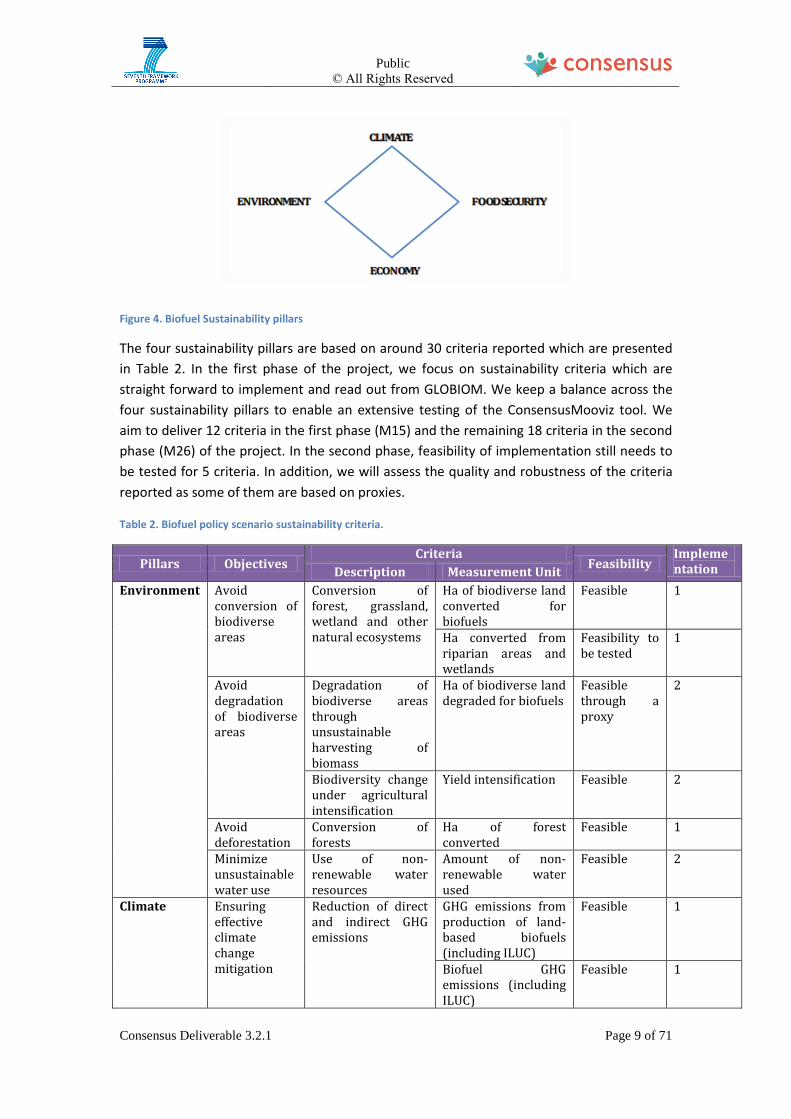
harmful impacts of biofuels on environment and food security worldwide. The GLOBIOM

model provides sustainability criteria around four main sustainability pillars which are

described in Figure 4.

Public



Figure 4. Biofuel Sustainability pillars

The four sustainability pillars are based on around 30 criteria reported which are presented

in Table 2. In the first phase of the project, we focus on sustainability criteria which are

straight forward to implement and read out from GLOBIOM. We keep a balance across the

four sustainability pillars to enable an extensive testing of the ConsensusMooviz tool. We

aim to deliver 12 criteria in the first phase (M15) and the remaining 18 criteria in the second

phase (M26) of the project. In the second phase, feasibility of implementation still needs to

be tested for 5 criteria. In addition, we will assess the quality and robustness of the criteria

reported as some of them are based on proxies.

Table 2. Biofuel policy scenario sustainability criteria.

Pillars Objectives Criteria

Feasibility Implementation Description Measurement Unit

Environment Avoid conversion of biodiverse areas

Conversion of forest, grassland, wetland and other natural ecosystems

Ha of biodiverse land converted for biofuels

Feasible 1

Ha converted from riparian areas and wetlands

Feasibility to be tested

1

Avoid degradation of biodiverse areas

Degradation of biodiverse areas through unsustainable harvesting of biomass

Ha of biodiverse land degraded for biofuels

Feasible through a proxy

2

Biodiversity change under agricultural intensification

Yield intensification Feasible 2

Avoid deforestation

Conversion of forests

Ha of forest converted

Feasible 1

Minimize unsustainable water use

Use of non-renewable water resources

Amount of non-renewable water used

Feasible 2

Climate Ensuring effective climate change mitigation

Reduction of direct and indirect GHG emissions

GHG emissions from production of land-based biofuels (including ILUC)

Feasible 1

Biofuel GHG emissions (including ILUC)

Feasible 1

Public



Food Security

Minimize impacts on land use

Land required for growing biofuels feedstocks

Ha of land used for food and energy crops for biofuels production

Feasible 1

Arable land expansion due to biofuel production

% increase of arable land due to expansion of food and energy crops for biofuel production

Feasible 1

Displacement of local food crops for biofuel production

Local food crops displaced by energy crops

Feasible 2

Avoid land rights violation

Land rights are not violated by large scale acquisitions (above 2000 Ha)

N. of people displaced


2

N. of land conflicts Feasibility to be tested

2

Minimize impacts on water use

Water required for growing biofuel feedstocks

Amount of water used in biofuel feedstock production

Feasible 2

Stress on water scarcity

Incidence of water used for biofuel production in water-stressed areas

Feasible 2

Avoid

competition

with food

demand

Displacement of local food crops for biofuel production

Local food crops displaced by energy crops

Feasible 2

Access to food at fair prices

Incidence of biofuel demand on food prices

Feasible 1

Reduce risks of increasing malnutrition and/or undernourishment (consumption of cheaper and/or less nutritious food).

Calorie intake for food used in biofuel production

Feasible 2

Calorie consumption per capita (i.e. vegetal, animal)

Feasible 1

Assess the net calories impact of biofuel production

Calorie supply into the food chain from animal feed co-products of biofuels

Feasible 2

Economy

Reduce dependency from fossil fuels

Energy security achieved through biofuels

% of energy substitution in transport due to biofuels

Feasible 2

Energy security achieved through other transport policy options (i.e. electric mobility etc.)

% of energy substitution in transport due to other renewables

Feasible 2

Ensure economic feasibility of biofuel policies

Cost of biofuel production

Production cost of biofuels

Feasible 2

Cost of public support to biofuels

Amount of public subsidies, tariffs and incentives per year


2

opportunity cost of Energy Feasibility to 2

Public



biofuel policy compared to GHG & energy savings through increasing energy efficiency of vehicles

savings/Investments costs

be tested

Ensure self-sufficiency of domestic production

Commercial balance Amount of imported biofuels

Feasible 1

Domestic production

Self-sufficiency level of feedstock production (net trade/total production)

Feasible 2

Balance spill-over effect in other sectors

Economic consequences/opportunity for farmers

Agricultural income Feasible 2

Amount of animal feed production associated to biofuels production

Feasible 1

Competition with food processor industries

Agricultural commodities prices

Feasible 1

2.3 Biofuel policy scenarios GLOBIOM is used to report sustainability criteria for biofuel assessment and quantify trade-

offs between different pillars using a scenario based approach. We apply GLOBIOM to

quantify a large number of biofuel policy scenarios and compare them to a benchmark, the

Reference scenario. The Reference scenario represents a “business as usual” scenario of the

global agricultural and forestry markets until 2050. However, in this scenario global biofuel

demand (1st and 2nd generation biofuels) is kept constant over time at 2010 volumes. By

comparing biofuel policy scenarios (with different biofuel targets) to the Reference (2010

volumes) we are able to quantify the impact of policies with respect to different objectives

and assess the sustainability of biofuels in 2030 and 2050. In what follows, we give an

overview of the Reference scenario assumptions and scenario drivers (Table 3) as well as the

biofuel policy scenarios.

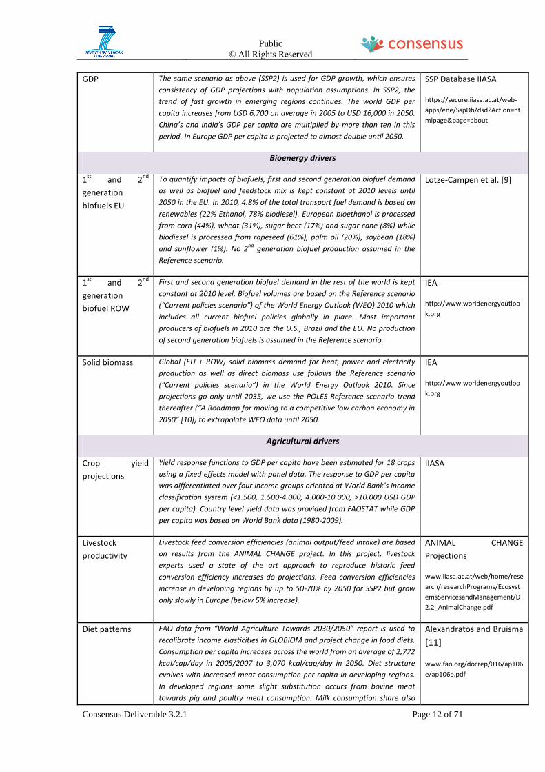
Table 3: Reference scenario drivers.

Variable Assumption Source

Macroeconomic drivers

Population The Shared Socio-economic Pathways (SSPs) are consistent and harmonized

prospective scenarios developed for the IPCC fifth Assessment Report. They

are widely used by the scientific community and include state of the art

projections for macroeconomic drivers (population and GDP growth). In

CONSENSUS we will use SSP2. The SSP2 scenario, called “Middle of the

Road” assumes mostly prolongation of currently observed trends and is a

business as usual scenario. World population in this scenario reaches 9.3

billion and stagnates inside Europe at around 500 million people by 2050.

SSP Database IIASA

https://secure.iiasa.ac.at/web-

apps/ene/SspDb/dsd?Action=ht

mlpage&page=about

Public



GDP The same scenario as above (SSP2) is used for GDP growth, which ensures

consistency of GDP projections with population assumptions. In SSP2, the

trend of fast growth in emerging regions continues. The world GDP per

capita increases from USD 6,700 on average in 2005 to USD 16,000 in 2050.

China’s and India’s GDP per capita are multiplied by more than ten in this

period. In Europe GDP per capita is projected to almost double until 2050.

SSP Database IIASA

https://secure.iiasa.ac.at/web-

apps/ene/SspDb/dsd?Action=ht

mlpage&page=about

Bioenergy drivers

1st

and 2nd

generation

biofuels EU

To quantify impacts of biofuels, first and second generation biofuel demand

as well as biofuel and feedstock mix is kept constant at 2010 levels until

2050 in the EU. In 2010, 4.8% of the total transport fuel demand is based on

renewables (22% Ethanol, 78% biodiesel). European bioethanol is processed

from corn (44%), wheat (31%), sugar beet (17%) and sugar cane (8%) while

biodiesel is processed from rapeseed (61%), palm oil (20%), soybean (18%)

and sunflower (1%). No 2nd

generation biofuel production assumed in the

Reference scenario.

Lotze-Campen et al. [9]

1st

and 2nd

generation

biofuel ROW

First and second generation biofuel demand in the rest of the world is kept

constant at 2010 level. Biofuel volumes are based on the Reference scenario

(“Current policies scenario”) of the World Energy Outlook (WEO) 2010 which

includes all current biofuel policies globally in place. Most important

producers of biofuels in 2010 are the U.S., Brazil and the EU. No production

of second generation biofuels is assumed in the Reference scenario.

IEA

http://www.worldenergyoutloo

k.org

Solid biomass Global (EU + ROW) solid biomass demand for heat, power and electricity

production as well as direct biomass use follows the Reference scenario

(“Current policies scenario”) in the World Energy Outlook 2010. Since

projections go only until 2035, we use the POLES Reference scenario trend

thereafter (“A Roadmap for moving to a competitive low carbon economy in

2050” [10]) to extrapolate WEO data until 2050.

IEA

http://www.worldenergyoutloo

k.org

Agricultural drivers

Crop yield

projections

Yield response functions to GDP per capita have been estimated for 18 crops

using a fixed effects model with panel data. The response to GDP per capita

was differentiated over four income groups oriented at World Bank’s income

classification system (<1.500, 1.500-4.000, 4.000-10.000, >10.000 USD GDP

per capita). Country level yield data was provided from FAOSTAT while GDP

per capita was based on World Bank data (1980-2009).

IIASA

Livestock

productivity

Livestock feed conversion efficiencies (animal output/feed intake) are based

on results from the ANIMAL CHANGE project. In this project, livestock

experts used a state of the art approach to reproduce historic feed

conversion efficiency increases do projections. Feed conversion efficiencies

increase in developing regions by up to 50-70% by 2050 for SSP2 but grow

only slowly in Europe (below 5% increase).

ANIMAL CHANGE

Projections

www.iiasa.ac.at/web/home/rese

arch/researchPrograms/Ecosyst

emsServicesandManagement/D

2.2_AnimalChange.pdf

Diet patterns FAO data from “World Agriculture Towards 2030/2050” report is used to

recalibrate income elasticities in GLOBIOM and project change in food diets.

Consumption per capita increases across the world from an average of 2,772

kcal/cap/day in 2005/2007 to 3,070 kcal/cap/day in 2050. Diet structure

evolves with increased meat consumption per capita in developing regions.

In developed regions some slight substitution occurs from bovine meat

towards pig and poultry meat consumption. Milk consumption share also

Alexandratos and Bruisma

[11]

www.fao.org/docrep/016/ap106

e/ap106e.pdf

Public



increases in diet.

In the biofuel policy scenario analysis, we implement different biofuel and land use policies

to quantify the impact of these policies with respect to different sustainability pillars. This

will be done by comparing a policy scenario to the Reference scenario using the

sustainability criteria as presented in above to quantify the impact on different sustainability

pillars. Table 4 presents the different biofuel policy scenario dimensions. Each scenario

dimension will be tested in all relevant combination resulting in more than 4.000 quantified

scenarios (e.g. Moderate, 10% biofuel share ethanol – High domestic production – Reference

scenario - Reference scenario – No deforestation – Medium biodiversity protection –

Reference scenario diets – Reference scenario yields).

Table 4. Scenario set-up for the biofuel policy scenarios quantified in phase 1 of Consensus.

Scenario driver Scenario description

EU biofuel policies 1. No biofuels, 0% biofuel share 2. Moderate, 10% biofuel share ethanol 3. Moderate, 10% biofuel share biodiesel 4. Moderate, 10% biofuel share 2

nd generation

5. Ambitious, 25% biofuel share ethanol 6. Ambitious, 25% biofuel share biodiesel 7. Ambitious, 25% biofuel share 2

nd generation

Source of EU biofuels 1. High domestic production 2. High imports from ROW

EU solid biomass 1. Reference scenario 2. Constant 2010 levels 3. EU ambitious target

ROW 1st

, 2nd

generation,

solid biomass

1. Reference scenario 2. ROW ambitious target

Land use change

regulations

1. Reference scenario assumptions 2. No deforestation 3. No grassland conversion and deforestation

Biodiversity protection 1. Reference scenario assumptions 2. Medium biodiversity protection 3. High biodiversity protection

Change in food diets 1. Reference scenario diets 2. Healthier diets globally 3. Western diets globally

Yield development 1. Reference scenario yield 2. Optimistic crop yield development

EU biofuel policies

While in the Reference scenario we keep European biofuel shares constant at 4.8% of total

transport fuel demand, we will quantify several European biofuel policy options by varying

the EU biofuel demand and biofuel mix. The biofuel shares in the scenarios range from 0%

Public



(hypothetical biofuel “phasing out” scenario) up to 25% in 2050 in the most ambitious

biofuel scenario.

In the “No biofuels” scenario we assume phasing out of biofuels after 2010. In a “10%

biofuel share” scenario we assume reaching the renewable energy targets as defined in the

Renewable Energy Directive [12] in 2020 and constant 10% biofuel shares thereafter. The

biofuel share in the ambitious scenario is based on the “Decarbonisation scenario under

effective technologies and global climate action” from the “Roadmap for moving to a

competitive low carbon economy in 2050” [10]. Here we implement a 10% share in 2020 and

assume a linear increase to 25% until 2050.

Projections of transport fuel demand (including public road transport, private cars and

motorcycles and trucks) are based on the “EU Energy, Transport and GHG Emissions Trends

to 2050: Reference Scenario 2013” [13]. Energy demand in the transport sector is projected

to remain constant at around 367 Mtoe until 2050 due to efficiency increases in the

transport sector. Besides the biofuel volumes, we also vary the biofuel mix across the

different scenarios. We differentiate between 3 different biofuel sources: bioethanol,

biodiesel and 2nd generation fuels (cellulosic feedstocks). While we keep the 2010 biofuel

mix (22% bioethanol, 78% biodiesel) until 2020 fixed [9], we assume a 100% shift to

biodiesel, bioethanol or cellulosic biofuels (2nd generation biofuels) in the different scenarios

until 2040/2050. Feedstock shares within a biofuel type are assumed to remain constant

across the different scenarios (see Table 3).

Source of EU biofuels

We quantify two different set-ups with respect to biofuel trade. In the “high domestic

production” scenario we assume that all biofuels consumed inside Europe are produced

domestically while in the “high imports from ROW” scenario we assume that additional

biofuel demand after 2010 is satisfied from biofuel imports only (thus biofuel production

inside Europe is kept at 2010 levels). However, even though we assume a different origin of

the processed biofuels, we do not make assumptions on the trade in biofuel processing

feedstocks.

EU solid biomass

In the Reference scenario set-up, EU solid biomass demand for heat, power, electricity

production and direct biomass use follows the World Energy Outlook 2010 (WEO2010)

“current policies scenario”. In the “constant 2010 levels” scenario we fix EU solid biomass

demand to 2010 volumes. In the “EU ambitious target” we follow the “450 scenario” from

the WEO2010 which represent a global 2 degree decarbonisation scenario with increased

bioenergy demand.

ROW first and second generation biofuels, solid biomass

In the Reference scenario set-up, the rest of the world solid biomass demand is based on

WEO 2010 “current policies scenario”. First generation biofuel demand is kept at 2010 levels

while no second generation biofuel production is assumed. In the “ROW ambitious target”

Public



bioenergy demand (first and second generation, solid biomass) follows the “450 scenario”

from the WEO2010 which represent a global 2 degree decarbonisation scenario with

increased bioenergy demand.

Land use change regulations

We assume different levels of land use change regulations globally to test if international

agreements could decrease or even mitigate potential negative impacts of EU biofuel

policies. While in the Reference scenario we allow for deforestation in developing regions

and conversion of grasslands globally (except inside the EU), we assume successful

implementation of land use regulations at global level in the two remaining scenario

variants. In the “no deforestation” scenario we assume no deforestation by 2020 while in

the “no grassland conversion and deforestation” scenario we also prevent conversion of

grasslands to e.g. cropland or short rotation tree plantations by 2020.

Biodiversity protection

In the Reference scenario, we don’t consider any protection of highly biodiverse areas

globally. We apply WCMC data [14] to delineate highly biodiverse areas in our land use

datasets. In the Carbon and biodiversity Report, six different biodiversity hotspots are

reported: Conservation International’s Hotspots, WWF Global 200 terrestrial and freshwater

eco-regions, Birdlife International Endemic Bird Areas, WWF/IUCN Centres of Plant Diversity

and Amphibian Diversity Areas. Global terrestrial biodiversity areas are identified wherever

four or ore more priority schemes overlap in the report. We follow this definition and

prevent conversion of highly biodiverse areas in the “medium biodiversity protection”

scenario by 2020. In the “high biodiversity protection” scenario, we even apply a stricter

definition and consider already areas where only two or more layer overlap as highly

biodiverse and prevent conversion.

Change in food diets

Calorie consumption per capita in the Reference scenario follows the FAO projections of

Alexandratos and Bruisma [11]. It increases across the world from an average of 2,772

kcal/cap/day in 2005/2007 to 3,070 kcal/cap/day in 2050. In the “healthier diets” scenario

we assume a shift towards less meat based diets around the world while in the “western

diets” scenario we assume a shift towards U.S diets globally with increased total calorie

consumption and meat demand.

Yield development

In the Reference scenario, productivity increases for the crop sector are based on

econometric analysis estimating crop specific yield response functions to GDP per capita

growth. In the “optimistic crop yield development” scenario we assume a more optimistic

development until 2050 with an additional 10% yield growth compared to the Reference

scenario.

Public



2.4 Prototype application The prototype delivered is a “small” toy model based on GLOBIOM. Even though the model

structure is similar, the prototype does not include the same level of detail in the different

sectors, supply chains or data sets. The prototype delivered is a small partial equilibrium

model of the agricultural sector including 4 regions (Europe, USA, Latin America and rest of

the world), 3 agricultural commodities (cereals, oilseeds and maize), 4 landcover types

(cropland, grassland, forests and other natural vegetation) and 1 biofuel supply chain

(oilseeds to biodiesel). Due to the limited representation of functionalities and accurate

data, prototype results are not representative and should not be used for any assessments

but should help understanding basic economic modelling principles and model behavior.

2.4.1 Installation

For the use of the GLOBIOM prototype GAMS software as well as a commercial solver

license is needed. GAMS is a free software available at http://www.gams.com. After

installation the license file has to be either copied in the local GAMS folder or read in after

starting GAMS by selecting “file” -> “options” -> “licenses”. Then, a standard solver for a

linear programming (LP) problem has to be selected. Therefore click CPLEX for LP problems

under “options” and “solvers”.

http://www.gams.com/

Public



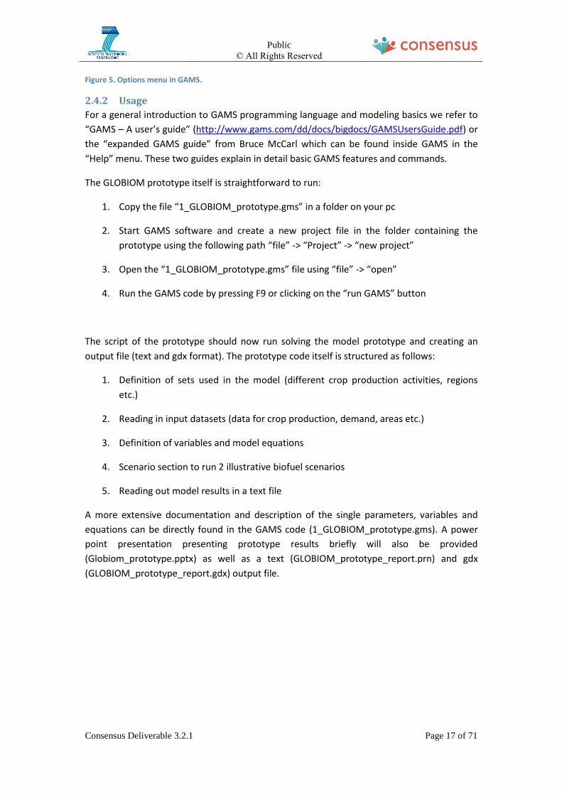
Figure 5. Options menu in GAMS.

2.4.2 Usage

For a general introduction to GAMS programming language and modeling basics we refer to

“GAMS – A user’s guide” (http://www.gams.com/dd/docs/bigdocs/GAMSUsersGuide.pdf) or

the “expanded GAMS guide” from Bruce McCarl which can be found inside GAMS in the

“Help” menu. These two guides explain in detail basic GAMS features and commands.

The GLOBIOM prototype itself is straightforward to run:

1. Copy the file “1_GLOBIOM_prototype.gms” in a folder on your pc

2. Start GAMS software and create a new project file in the folder containing the

prototype using the following path “file” -> “Project” -> “new project”

3. Open the “1_GLOBIOM_prototype.gms” file using “file” -> “open”

4. Run the GAMS code by pressing F9 or clicking on the “run GAMS” button

The script of the prototype should now run solving the model prototype and creating an

output file (text and gdx format). The prototype code itself is structured as follows:

1. Definition of sets used in the model (different crop production activities, regions

etc.)

2. Reading in input datasets (data for crop production, demand, areas etc.)

3. Definition of variables and model equations

4. Scenario section to run 2 illustrative biofuel scenarios

5. Reading out model results in a text file

A more extensive documentation and description of the single parameters, variables and

equations can be directly found in the GAMS code (1_GLOBIOM_prototype.gms). A power

point presentation presenting prototype results briefly will also be provided

(Globiom_prototype.pptx) as well as a text (GLOBIOM_prototype_report.prn) and gdx

(GLOBIOM_prototype_report.gdx) output file.

http://www.gams.com/dd/docs/bigdocs/GAMSUsersGuide.pdf

Public



3 Transport modeling framework

3.1 Introduction Modelling has the potential to provide the transport sector with a “quantified understanding

of current and future issues” [131]; as such it is an important component of the

development and assessment of transport policies (usually ex ante evaluation). The key

consideration when developing a transport model to support the ex-ante evaluation of

alternative policy options is that model’s set-up takes place within the overall evaluation

process [105], [122], [131], [162]. This requires an ordered process, including: (a)

appreciation of the range of modelling techniques available, (b) establishment of a clear

policy context (in terms of purpose and alternative policy options), (c) development of a

clear assessment context (in terms of the desired outcome and the evaluation objectives)

and (d) review the potential for different modelling techniques to support the specific

policy’s assessment requirements.

Following such a process, a transport model has been developed in the framework of

Consensus, tailor-made for the evaluation of the Consensus transport policy scenario (road

pricing). The transport model is presented in this chapter, organized in two main sections:

In section 3.2 a short State-of-the-Art review on transport modelling techniques is

presented; first in general and then focused road pricing policies to ultimately

provide a suitable synthesis of existing techniques.

In section 3.3, policy and assessment context is presented and model’s purpose and

desired outputs are clearly identified; then model’s type (modelling technique) is

decided, based also on the State-of-the-Art review, its role into Consensus

framework, structure/operation and development stages are outlined. Finally, in

sub-sections 3.3.2 to 3.3.5 model’s development stages, structure and operation

(including a simple user guide) are analyzed, including reference to the respective

data requirements1.

3.2 State-of-the-Art review

3.2.1 Modelling techniques in transport sector

Transport models are predominantly used to predict transport demand under specific

conditions’ changes (i.e. infrastructure provision, management measures implementation,

pricing instruments enforcement). Two main model types are commonly used, namely:

- Conventional, four-step transport models; the most well-known and commonly used in

practice.

- Simplified models; usually applied to make rapid progress in particular circumstances.

1 The analytical data requirements are presented in Deliverable “D2.3.1 – Domain Data Sources”.

Public



Conventional models tend to be complex, time and data consuming [131], [172] and more

dedicated in analyzing “operational characteristics” [137], but when it comes to testing

demand management options or price-based measures, conventional transport models are

limited and other approaches are needed [102], [189].

Simplified models represent the transport system with a high degree of network and zonal

aggregation and produce mainly “indicative” or “approximate” forecasts, rather than

conventional transport models, which attempt to provide “precise” or “accurate” results

[157]. Three main types of simplified models exist [131], [145], [152], [192]:

- Simplified demand models: Mode choice models, Elasticity based models

- Structural models: Generalized relationship models, Regression based models.

- Sketch planning models

Simplified models have a number of comparative strengths [131], including: greater

segmentation of demand type, behavior and dynamic aspects than is normally possible in

conventional models, speed and low cost of use, transparency, ease of understanding and

use and testing flexibility and accessibility. A great number of simplified models have been

developed internationally [115],[116],[117], [123], [145], [156], [157], [181], [182].

3.2.2 Modelling practices for estimating the impacts of road pricing

Currently, there is no standard approach for representing tolls in travel demand models

[170], [187] and there is no consensus as to the best methods for developing traffic (and

revenue) forecasts when examine road pricing implementation [147]. The choice of

modelling technique varies, according to the intended application/s, the available resources

and availability of calibration and/or validation data [119], [170]. A review of current

practices for road pricing applications identified five major categories of modelling

procedures [169], [170], [179]:

- Activity-based modelling procedure, which allows pricing to be included explicitly into

the decision hierarchy. Often, constraints of time and cost limit the ability to gather the

data needed in research.

- Mode choice; car trips on a tolled or non-tolled road are considered as distinct modal

choices within an existing four-step model, with separate modal split functions for work

(or work-related) and non-work trip purposes.

- Trip assignment models are used to estimate and forecast route choice decision

assuming that trip distribution and modal share remain unchanged in the absence of

feedback loops. They are usually applied within an existing four-step model.

- Diversion models that calculate the market share of travellers who would use a toll

facility at varying levels of toll charges. They are used predominantly by transportation

consulting firms who develop toll revenue forecasts for investment decisions.

Public



- Sketch planning methods, which are quick-response tools for project evaluation. They

are often spreadsheet-based techniques that apply similar to conventional models

concepts to aggregated or generalized data. Because of their flexibility, these tools are

often developed by agency staff or consultants for a specific project.

3.2.3 Modelling assumptions and data requirements in road pricing analyses

Regardless of the modelling procedure used, a common underlying assumption exists; the

one that travellers make economically rational choices in deciding where to go (destination

choice), what means of transportation to use (mode choice), and what route to take (route

choice). In other words, all modelling processes assume that travellers choose among a set

of alternatives and select those having the lowest generalized cost (a combination of

monetary and non-monetary costs of a journey) [170]. The generalised cost is equivalent to

the price of the good in supply and demand theory, and so demand for journeys can be

related to the generalised cost of those journeys using the price elasticity of demand. Supply

is equivalent to capacity (and, for roads, road quality) on the network.

In economic theory, it is well established that there is an inverse relationship between

demand and cost [138], [149], else the price elasticity of demand (for travel) is negative. As

such, changes in generalised cost of travel cause inverse changes in demand for travel and

this latter mentioned change is usually calculated using the respective elasticity. Since most

benefits/costs from interventions/ changes in transport system result from generalized cost

changes [184], transport models basing demand forecasts on generalized cost changes can

provide relatively straightforward quantitative estimations of dominant benefit/cost

categories i.e. safety impacts, environmental impacts etc.

3.3 Modelling framework for the Consensus transport policy

scenario – prototype description and application

3.3.1.1 Policy and assessment context

There are two main goals behind road pricing as identified by transport economists [160]

[186] and adopted by the EU: funding of Europe’s vital road infrastructure (mainly Trans-

European road network) and sustainable use of road transport infrastructures currently

affected by congestion and consequent problems [110], [159]. Despite the fact of the EU

encouraging its member states to include road pricing in their political agenda, one of the

basic challenges in all governmental levels, is to seek a “balanced way” to do that.

A “balanced way” basically implies the development of a coherent assessment framework to

support the evaluation of all (possible/applicable) alternative road pricing policy options

against often conflicting policy objectives and (hopefully) the identification of the most

optimal one. Both possible road pricing options and policy objectives are presented below in

Table 5 and Table 6. Table 5 summarizes the components of road pricing policy options,

applicable/suitable only on a “project basis” level.

Public


Consensus Deliverable D.3.2.1 Page 21 of 71

Table 5. Alternative Scenarios Components2 (road pricing policy schemes including road project development options and details)

RP policy

type

Project

type

Implementation

Scales

Application

Areas

Roadway Characteristics Responsible

Authority

Toll/Charge

Collection Techniques Price structure

Length Lanes

Road tolls

(fixed/flat

rate)

- New - Upgrade of

existing

- Spot - Facility - Corridor

- Interurban - Urban3

- <= 20 km - 20-45 km - 45-75 km - 75-100 km - > 100 km

- 2L/dir. - 3L/dir. - 3+L/dir.

- Public - Private

- Toll booths - ETC - Toll booths & ETC

F € /in bound trip

(variant according to vehicle

type; discount can be assumed

for frequent users of ETC)

Distance-

based

charging

- New - Upgrade of

existing

- Corridor - Interurban - Urban

- <= 20 km - 20-45 km - 45-75 km - 75-100 km - > 100 km


- Public - Private

- Toll booths - ETC - Toll booths & ETC - OVR - ETC&OVR - GPS/GNSS - ETC&GPS/GNSS

F €/km traveled


type; discount can be assumed

for frequent users of ETC)

Congestion

charging

- Upgrade of existing

- Spot - Facility - Corridor

- Urban - <= 20 km - 20-45 km - 45-75 km - 75-100 km - > 100 km


- Public - Private

- Pass F €/in bound trip


type)

- ETC - OVR - ETC&OVR - GPS/GNSS - ETC&GPS/GNSS

F €/in bound trip


type and period of day –peak

hour-; discount can be

assumed for frequent users of

ETC)

2 Definitions of the various components can be found in Deliverable 2.1.1 – User Requirements

3 For urban areas, there is a further differentiation to small and large urban areas according to population, which takes place in the model.

Public



The “project basis” option resulted through Stakeholders’ consultation (in WP2/WT2.1-User

Requirements) and is in line with one of the EU’s primary consideration to use road pricing

as the basic funding mechanism for Trans-European road network (motorways and high-

quality roads, whether existing, new or to be adapted) development and maintenance.

Each road pricing policy alternative is basically a (different) combination of the following

components:

1. The project type

2. The project scale, further differentiated by length and typical cross-section

3. The application area, further differentiated by population size

4. The type of authority, responsible for operation

5. The road pricing types

6. The toll collection techniques and

7. The price level and structure

Since the purpose is to examine policy options for a specific/given project -and not examine

also alternative project options-, for any scenario under investigation the upper half of the

components list (1) to (3) will be fixed (i.e. the project is given and will not change); and the

optimal road pricing policy alternative is searched by searching optimal (combinations of)

parameters in the bottom half of the components list (4) to (7).

The set of objectives presented in Table 6 summarizes the most relevant (see [110], [111],

[112], [128], [142], [143], [146], [150], [153], [155], [159], [167], [171], [177], [185], [186],

[188]) objectives (including metrics) for the comparative evaluation of the alternative road

pricing policy options.

Table 6. Objectives and their metrics for road pricing schemes evaluation

Objectives Metrics Metrics Measurement

(type; units)

RP economic feasibility Relative investment cost Qualitative;

Verbal Scale:

5- Very Low,

4- Low,

3- Medium,

2- High,

Public



1- Very High

RP financial viability Relative Operational Cost Quantitative;

in % of gross revenues

Reduce traffic

congestion

Increase in Level of Service Quantitative;

% decrease of ratio Traffic

Flow/Capacity

Improve safety Reduction of accidents costs Quantitative;

in % decrease of accident costs

Improve air quality Reduction of air pollution

external costs

Quantitative;

in % decrease of air pollution

external costs

Reduce noise

annoyance

Reduction of noise external

costs

Quantitative;

in % decrease of noise external costs

Ensure user

convenience

User convenience level in

using the RP system

Qualitative, Verbal Scale:

5- Very High,

4- High,

3- Medium,

2- Low,

1- Very Low

Ensure social

fairness/equity effects

Availability of alternative

modes and/or routes for

transport

Qualitative;

Verbal Scale:

4- Availability of both routes and

other modes,

3- Availability of other routes but

not other modes,

2- Availability of other modes but

not routes,

1- No available routes or modes,

The combinations of Table 5 components can produce thousands of scenarios. Adding to

that the multiple –and often conflicting- objectives of Table 6 it is acknowledged that

decision-making in the case of Consensus road pricing policy scenario is a complex and

Public



rather challenging procedure. Nonetheless, ConsensusMOOViz tool could significantly

reduce this complexity as long as the policy context parameters are well structured, well

defined and of course valued. In this framework, the purpose of the transport model is to

provide the necessary input to the ConsensusMOOViz tool for the comparative assessment

of the performance of the alternative road pricing policy scenarios against the policy

objectives. To this end the desired outputs of the transport model will be the absolute -and

where not possible approximate yet comparatively reliable- estimates of the objective’s

metrics for each alternative road pricing policy scenario.

3.3.1.2 Transport model type, role, structure, outline and development stages

Review of the State-of-the-Art of the various modelling techniques leads to the following

main conclusions:

- the inherent structure of conventional models tends to make them unsuitable for testing

road pricing policy options (at least not without substantial modification)

- simplified models and especially diversion (post processor) models or sketch planning

methods are considered more flexible, quick-response, easy to understand and use

(especially for a specific project)

- regardless of the modelling procedure used, two common underlying assumptions exist;

travellers make economically rational choices (based on generalized cost of travel) and

there is an inverse relationship between travel demand and generalized cost of travel

Based on the above and bearing in mind Consensus road pricing policy scenario specificities:

- the “project basis” implementation level, where road pricing policy concerns imposing

tolls on a specific project (either a new project or the upgrade of an existing roadway)

- the rather limited time-frame during, Consensus project, for modelling procedures and

the lack of a readily available (sophisticated) software

- the quantity and quality of publicly available data and literature/research/case studies,

especially on transport models basing demand forecasts on generalized cost changes

using respective elasticities

The Consensus transport model was decided to be a “simplified” sketch model tailor-made

for (the generic case of) a new road project or for the upgrade of an existing roadway,

adopting diversion models’ technique and assuming that main demand drivers are roadway

capacity and generalized cost of travel. The model produces/ forecasts changes in demand

using the selected drivers changes as well as respective elasticities.

Since half of the policy objectives presented in Table 6 (Reduce traffic congestion, Improve

safety, Improve air quality and Reduce noise) are demand oriented or demand related, the

forecasted changes in demand can provide relatively straightforward quantitative

estimations of these policy objectives. For the rest of the objectives domain data will be

Public



analyzed and qualitative valuations will be provided through the model based on statistics

and -where needed- on domain experts opinions.

The role of transport model in the overall road pricing policy assessment framework of

Consensus, and the schematic outline of its structure/operation is presented in Figure 6.

Figure 6. Road Pricing Model Role and Structure

In order for the transport model to fulfill its role into the overall road pricing policy

assessment framework and to reach the presented structure, an ordered process of five

main stages of development –before application- was followed (see also Figure 7).

- Perceptual stage: It aims at developing the perceptual process that is a general

understanding of road pricing policy alternatives’ possible impacts on each objective.

- Conceptual stage: In this stage, perceptual processes are described and simplified by

equations based on transport literature and practice, i.e. default values and/or

coefficients of parametric equations.

- Computing stage: This third stage involves transferring the conceptual process to

computer code. The main product of this stage is a spreadsheet-based model that can

be used to efficiently produce estimates of the selected objective’s metrics, for each

alternative road pricing policy scenario.

- Calibration stage: The fourth stage is calibration, which contains both, the choice of

appropriate objective functions to evaluate the model and the choice of suitable

optimisation methods to explore the model parameter space and to eventually find

feasible model parameterisations.

- Validation Stage: The term validation usually refers to the test of a model with

independent data.

Public



The decomposition of the modeling process was also necessary for the identification of data

requirements4.

Figure 7. Model Development Stages

3.3.2 Perceptual stage

The main immediate5 impacts’ chains of road pricing are presented next.

3.3.2.1 Road pricing impacts on travel costs

The direct economic impact of road pricing is a rise in travel and freight costs (Figure 8).

Figure 8. Impacts of road pricing on travel and transportation costs (Source: CEDR, 2009)

4 Analytical description of data requirements, along with their utility and availability can be found in

the respective deliverable “D2.3.1 – Domain Data Sources”.

5 The long-term impacts are not analyzed; they are considered controversial and unlikely to

undermine the immediate effects [113], [124], [126]

Public



This affects in turn the volume of trips and deliveries or the routing of trips and deliveries. If

pricing is scaled/differentiated according to the time of day and/or by the characteristics of

vehicles, there will also be an impact on the timing of travel and deliveries and maybe on the

characteristics of the vehicles used [110].

3.3.2.2 Road pricing impacts on road networks functionality

Since road pricing has an impact on travel behavior and freight patterns, it affects the

functionality of transport links (Figure 9).

Figure 9. Impacts of road pricing on road network functionality (Source: CEDR, 2009)

Pricing can affect the volume, the distance traveled, the timing of travel as well as the modal

split or the route choice on local networks [106]. Functionality improvements take place if

congestion or stop-and-go traffic during peak hours is reduced. As the flow of traffic

improves, travel times and vehicle operating costs reduce, thereby outweighing the cost

impact of charges [110]. Also, travel times become more predictable and travel planning is

easier, which in turn causes further time savings as travelers have fewer needs to budget

additional time to avoid late arrival [113].

3.3.2.3 Road pricing impacts on traffic safety

Road pricing can have both positive and negative impacts on traffic safety [125], [127]

(Figure 10). It is acknowledged that there is an almost proportional increase in the number

of accidents with increasing traffic volumes [107]; so if road pricing reduces overall traffic

flows it is likely to lower accidents risks and accident numbers [113]. On the other hand,

drawbacks may also occur. Some drivers may avoid tolls by using un-tolled, higher risk

routes. In addition, rising average speeds may result in more serious accidents even if the

overall number of collisions decreases.

In general, traffic safety usually improves when new high-quality infrastructures (e.g.

motorways) replace existing poorly functioning links in the network. If the investments are

financed by charges, a link between road pricing and traffic safety is created [110].

Public



Figure 10. Impacts of road pricing on traffic safety (Source: CEDR, 2009)

3.3.2.4 Road pricing impacts on the environment

Each vehicle trip produces emissions and noise [140]. The main environmental potential of

road pricing (regarding emissions and noise) is its ability to relieve congestion and improve

the smoothness of traffic (Figure 11) [110].

Figure 11. Impacts of road pricing on the environment (Source: CEDR, 2009)

3.3.2.5 Road pricing impacts on the travel convenience

Convenience of travel is a subjective impact closely related to functionality (Figure 12). In the

case of charges (especially tolls that cut peak traffic), the discomfort due to poor

functionality reduces and travel experiences improve [110]. Convenience is also connected

with the technology used for toll collection [186].

Public



Figure 12. Impacts of road pricing on travel convenience (Source: CEDR, 2009)

3.3.2.6 Road pricing impacts on road funding

In most countries, road funding primarily relies on the state budget, which is to a varying

degree supported by taxes collected from the road sector (Figure 13). This situation is

changing as road pricing revenues are increasingly used to fund roads. In some cases, the

funding of individual projects relies completely on revenue from road pricing (e.g. tolled

motorway links, bridges, and tunnels) [110], [193].

It is important to understand that in the case of road pricing, funding and demand

management may sometimes be opposing objectives [186] and as such the appropriateness

of price level depends on the desired balance of the objectives.

Figure 13. Impacts of road pricing on road funding (Source: CEDR, 2009)

To summarize, since people make economically rational choices when it comes to travel

[170], road pricing will virtually always affect travel decisions like destination choice, mode

choice, route choice and frequency of trips, not to mention even making the trip or not

[148]. Making of these choices, will certainly affect a number of factors including amount of

Public



travel and mobility itself, socio-economic impacts of travel (i.e. congestion, accidents,

environmental impacts, quality of life), economic impacts (i.e. production of companies,

employment) even public budget.

3.3.3 Conceptual stage

Based on the underlying modelling assumptions as well as perceptual stage’s notions, in the

conceptual stage forecasting process is described and simplified where needed by equations.

It should be mentioned that Consensus model as all simplified sketch models has limitations

and its results will always contain uncertainties, no matter how sophisticated this may be

[180].

3.3.3.1 Algorithms

The basic equations of this stage include:

- Demand drivers’ estimation; mainly generalised cost (incl. travel time cost and vehicle

operating costs),

- Demand changes estimation; as a function of specific drivers/factors affecting it

(generalised cost and roadway capacity) as well as respective elasticities of demand,

- Demand-related impacts (safety and environmental) estimation, per vehicle category

and network type, based on demand changes and impacts’ unit values.

Based on the above equations, the demand-related objectives presented in Table 6 are

valued. For the estimation of the non-demand related objectives’, direct valuation on an

artificial scale takes place using simple utility functions and readily available data and/or

opinions of domain experts. In general, data requirements of the Conceptual stage, along

with their utility and availability can be found in the respective deliverable “D2.3.1 – Domain

Data Sources”.

3.3.3.1.1 Demand drivers

The development of an analytical model to estimate the likely ‘capture’ (in percentage

terms’) of in-scope traffic by toll roads requires the conversion of all costs and benefits in the

same units. In particular, time and money needed to be converted to the same currency

often termed “generalized cost”. As part of this process, a “Value of Time” (VoT) is calculated

for all the key behavioral segments in the model.

An improvement in supply conditions due to for example an improvement in the corridor

capacity leads to a reduction in equilibrium generalized cost. To define generalized cost;

generalized cost is an amount of money representing the overall disutility (or inconvenience)

of traveling between a particular origin (i) and destination (j) by a particular mode (m) [187].

In principle, this incorporates all aspects of disutility including the time given up, money

expenditure and other aspects of inconvenience/discomfort, but in practice the last of these

is usually disregarded.

For travel between (i) and (j) the user benefit is estimated by:

Public



Where ‘I’ indicates the do-something scenario (in our case the proposed project, either this

is an upgrade of an existing roadway or a new corridor) and ‘0’ the do-nothing (the base

case).

A useful approach in explaining travel choices is to relate demand to a generalized cost

which incorporates various important elements.

Generalized cost function

Generalized cost function should be considered a linear function of its component variables.

More specifically, the travelers’ generalized cost (Equation 3-1) is a linear additive function

of Level-of-Service (trip length, time) and price components (direct monetary costs such as

tolls charged) related to the perceived disutility of travel. The components of the journey are

weighted by parameters which are compiled (e.g. km-costs), or perceived by the traveler

(e.g. value of time). Generalized costs in are differentiated by vehicle type (passenger cars,

trucks) - and trip purposes (commuting, all other) for the variable of ‘value of time’-.

TollDc ijij

tpm

ij ** 21

, (Eq. 3-1)

where

tpm

ijc , : generalised cost of travelling from zone (i) to zone (j), by vehicle type (m) for

purpose (tp).

1 : value of time, for vehicle type (m) and trip purpose (tp)

ij : travel time from zone (i) to zone (j).

2 : vehicle operating cost for vehicle type (m)

ijD : distance from zone (i) to zone (j).

Toll : any toll encountered by a trip from zone (i) to zone (j), for vehicle type (m).

m : vehicle type, m= passenger car, truck

tp : trip purpose, tp = commuting, other

Values of time for car users

Values of time for passenger car users are usually estimated based on Stated Preference (SP)

surveys. Plenty of research projects and studies (UNITE, IWW/INFRAS, OSD, GRACE, HEATCO,

IMPACT) summarized and further analyzed scientific and practitioner’s knowledge on the

issue in order to ultimately recommend a set of values of time. The HEATCO study being one

of the most complete, recent and officially suggested by the EC was also chosen in the

framework of Consensus. The HEATCO study provides unit values for time in

Public



(€/passenger/hour), for each EU country, for different trip purposes (in 2002 values) [136;

Table 0.3, pg. S9].

HEATCO values, converted into 20126 values, are presented in also included in the

(background) databases supporting Consensus model operation.

Table 7 and also included in the (background) databases supporting Consensus model

operation.

Table 7. Car Values of Time, for different trip purposes, in European countries (€/passenger/hour, in 2012 prices)

Country Business Commute Other

Austria 32,44 10,48 8,78

Belgium 30,64 9,78 8,20

Cyprus 24,91 10,70 8,97

Czech Rep. 18,04 8,30 6,95

Denmark 32,99 10,12 8,49

Estonia 17,60 7,82 6,55

Finland 31,98 9,83 8,25

France 30,16 13,62 11,42

Germany 30,51 10,05 8,43

Greece 19,77 8,06 6,76

Hungary 15,23 6,49 5,45

Ireland 35,19 11,29 9,47

Italy 25,58 11,58 9,71

Latvia 15,77 6,99 5,86

Lithuania 16,42 7,17 6,02

Luxembourg 45,79 16,38 13,74

Malta 21,58 8,63 7,23

Netherlands 30,44 9,64 8,09

Poland 17,85 7,82 6,56

6

Data on Harmonised Index of Consumer Prices (HICP) (2000-2012) were used to update unit Values of Time.

Public



Portugal 19,40 7,66 6,42

Slovakia 17,76 7,55 6,34

Slovenia 22,21 10,85 9,10

Spain 25,03 10,90 9,15

Sweden 36,29 11,22 9,41

UK 32,62 10,70 8,97

Switzerland 37,94 14,75 12,36

Values of time for commercial vehicles (trucks)

Values of time for heavy goods vehicles have been derived from a research of the Greek

road freight industry [144], which reviewed also similar researches in other countries.

Evidence suggests that the Values of Time for commercial operators are somewhere

between 1 and 2.5 times the drivers salary, depending on type of industry and operating

costs.

Another way to approach the issue is by comparing the Values of Time for commercial

vehicles with that for cars. Studies carried out in the UK, Portugal, Turkey and Argentina

[144] (see Table 8) suggest that the value of time for trucks lies between 1.1 and 2.2 times

that for cars.

Table 8. Comparison of truck and car Values of Time

Country Truck/Car business Truck/Car average

UK 2.0 3.4

Portugal 1.3

Turkey 1.9

Argentina 1.1 small- 2.2 large

Poland 1.75-2.5

Referring to the above table, high “multipliers” such as those in the UK arise only when there

are many large operators and “just-in-time” delivery contracts. A safer approach would

assume a value of time at the lower end of the range. In this framework, the following values

of time were chosen to be used in the Consensus model - for the average truck-:

- Small company and own-truck operators = (1.5)*(car VoT)

- Medium to big freight companies= (2.5)*(car VoT)

Public



Vehicle operating costs

Vehicle operating cost is heavily dependent on the road geometry and road operational

characteristics, travel speed and pavement condition. Vehicle operating costs include costs

for fuel, maintenance, tyre replacement, depreciation, tax and insurance.

To derive vehicle operating costs the methodology proposed by Poriotis and Vakirtzidis [161]

was used, where vehicle operating cost is calculated as a function of the average travel

speed for each vehicle type, using the following equation:

cVbVaVOCm ** 2 (Eq. 3-2)

where

VOCm : vehicle operating cost, for vehicle type (m)

V : vehicle’s speed (in km/hour)

a,b,c : parameters dependent on vehicle’s technical characteristics, and are:

Parameters’ values for.. Passenger Cars Trucks

a 0,00002914 0,000135

b -0,00502432 -0,017436

c 0,4256765 1,426324

3.3.3.2 Forecasting demand changes

As already mentioned, Consensus model adopts diversion models’ technique, as such the

model presented does not account for “induced traffic”. It only accounts for generated

traffic. Generated traffic is the additional vehicle travel that results from a road

improvement, particularly expansion of congested urban roadways [151]. The upgrade of an

existing corridor or the construction of a new corridor/facility/spot usually leads to

generalised cost reductions. Shortly after the road improvement, new traffic is generated

coming from other routes, times or modes.

New motorways, especially those in heavily congested urban areas, can have levels of

growth higher than those expected; this extra traffic is called “induced traffic”. However,

usually existing land use (e.g. location of residence or work) constrains such behavioural

changes, on most trunk road schemes induced traffic impacts resulting from such changes

are likely to appear progressively and be limited to the long term (10 or more years).

Furthermore, in most cases, although the new schemes are expected to create significant

reduction in travel time, the timesaving benefits will be outweighed by the higher tolls;

consequently, induced traffic will be limited.

A number of sensitivity tests were run using the Road Transport model, comparing the Do-

nothing and the Do-Something and the increase in the number of trips arising due to

Public



elasticity application on the generalised cost by trip purpose was estimated less than 2%.

Therefore, it was decided to ignore induced traffic, as the impact on revenues would be

negligible.

Forecasting traffic demand changes

The key assumption of Consensus transport model, when forecasting demand, is that

demand (Y) changes, due to roadway improvements and/or conditions changing, are

estimated based on changes of two main demand drivers (factors/variables affecting

demand), capacity (CP) and generalized cost (c) (see general Equation 3-3)

CPcf , (Eq. 3-3)

Key piece of information needed for travel forecasting, in the absence of a 4-stage traffic

model, are the elasticities. The elasticities provided in this project are the outcome of a very

wide literature review and cover various studies from different geographical locations [103],

[108], [109], [114], [118], [120], [121], [132], [133] [134], [154], [163], [164], [165], [166],

[168], [173], [174], [176], [190], [191].

Consensus model uses travel demand elasticities (measured in vehicle-kilometers travelled)

with respect to capacity and generalized cost, to estimate new travel that may be generated

over and above traffic that is simply rerouted from other highways. This includes new trips

generated or attracted to new development, and existing trips diverted from other

destinations.

An elasticity of demand with respect to capacity of 0.2 and an elasticity of demand with

respect to generalized cost of -0.31 were assumed in the Road Transport model. These

values were the average of the range of (each) demand elasticity, found in the literature

referenced above. The approach taken to determine changes in demand levels due to

changes in capacity and generalized cost is based on the PDFH approach [101]. A very brief

outline of this approach is presented in this chapter (for more details refer to Arup’s study

[101]). The main idea behind this approach is presented in Figure 14.

Figure 14. Schematic of basic PDFH-style forecast (Source: Arup & Oxera, 2010)

To estimate/forecast the level of new demand, an index of the ratio of new demand to

previous demand is calculated. The index is then applied to an existing demand level to

determine the forecasted value of new demand after the roadway improvement and pricing

Change in

demand driver

(ratio)

Raise to power

of elasticity

Growth Index

Multiply by

base demand

Forecast demand

Public



policy implemented. In the Road Transport model, where demand is changed due to changes

in generalized cost and capacity levels, the formula of the index is given below in Equation 3-

4 and then Equation 3-5 is used to forecast the new demand:

cCP El

m

BC

m

P

El

BC

P

c

c

CP

CPI

..

(Eq. 3-4)

m

BC

m

P YIY (Eq. 3-5)

where:

I : index ratio

PCP : roadway section capacity, for proposed project

BCCP : roadway section capacity, for base case situation

m

Pc : generalised cost of travelling by vehicle type (m), for proposed project

m

BCc : generalised cost of travelling by vehicle type (m), for base case situation

CPEl. : elasticity of demand (in vehicle-kilometres travelled) with respect to roadway

capacity

cEl. : elasticity of demand (in vehicle-kilometres travelled) with respect to generalized

cost of travel


m

P : demand (in vehicle-kilometres travelled) by vehicle type (m), for proposed project

m

BC : demand (in vehicle-kilometres travelled) by vehicle type (m), for base case situation

Index and demand in equations 3-4 and 3-5 respectively, are estimated first by vehicle type

and then they are aggregated. The basic result of equation 3-5 is forecasted demand in

vehicle-kilometers travelled. Nonetheless, it can be transformed into traffic flow as well (in

vehicles).

3.3.3.3 Demand related objectives

Reduce traffic congestion (OBJ.3)

The reduction of traffic congestion is planned to be measured through increase of the level

of service and more specifically as the decrease (in %) of the "Volume-Demand-to-Capacity

Ratio c

v . Volume-Demand-to-Capacity Ratio is a measure that reflects mobility and quality

of travel of a roadway facility or a section of a facility. It compares roadway demand (vehicle

Public



volumes) with roadway supply (carrying capacity) and is generally reported as a decimal, i.e.

0.8 or 1.2 and then categorized into a level of service ranging from A (free-flowing) to F

(extremely congested). It is a common performance measure and is widely used in models

and transportation studies.

The estimation of “reduce traffic congestion” objective is given in Equation 3-6.

%3.

BC

BC

BC

BC

P

P

OBJ

cv

cv

cv

(Eq. 3-6)

where

AOBJ.3 : is the estimated value of “reduce traffic congestion” objective

vP : traffic flow (vehicles/hour/lane) of proposed project, during peak hour

vBC : traffic flow (vehicles/hour/lane) of base case situation, during peak hour

cP : capacity (vehicles/hour/lane) of proposed project

cBC : capacity (vehicles/hour/lane) of base case situation

Improve safety (OBJ.4)

The improvement of traffic safety is planned to be measured through reduction of accidents

costs and more specifically as the decrease (in %) of accidents costs. As outlined in the

Perceptual Stage there is an almost proportional increase in the number of accidents with

increasing traffic volumes [107] as well as with the amount of travel in terms of frequency

and/or distance traveled. It is also acknowledged that accident numbers deteriorate social

welfare through property damages, injuries, or loss of life [113].

Plenty of research projects and studies (UNITE, IWW/INFRAS, OSD, GRACE, HEATCO,

IMPACT) summarized –and further analyzed- scientific and practitioner’s knowledge on the

issue in order to ultimately recommend a set of methods and default values for estimating

accidents and other external costs for the case of conceiving and implementing transport

pricing policies and schemes. The IMPACT study being the most recent and officially

suggested from the EC was also chosen in the framework of Consensus. IMPACT study

provides unit values for accidents in (€ct/vkm), for each EU country, for different network

types and different vehicles categories (in 2000 values) [107; Table 10, pg. 44].

IMPACT values, as updated into today’s7 values, are presented in Table 9 and also included in

the (background) databases supporting Consensus model operation.

7 Data on Harmonised Index of Consumer Prices (HICP) were found for the period 2000-2012 and

were used to update accidents costs unit values.

Public



Table 9. Unit values for accidents in European countries (in €ct/vkm) – for main network types and vehicle categories

Passenger Cars Trucks

Country Urban Interurban Motorways Urban Interurban Motorways

Austria 7,28 2,77 0,52 18,52 4,67 0,52

Belgium 8,58 3,27 0,61 21,86 5,51 0,61

Cyprus 6,88 2,61 0,49 17,52 4,42 0,49

Czech Rep. 4,46 1,70 0,32 11,36 2,87 0,32

Denmark 5,67 2,16 0,41 14,44 3,64 0,41

Estonia 5,17 1,96 0,37 13,17 3,32 0,37

Finland 4,33 1,65 0,32 11,03 2,79 0,32

France 8,41 3,21 0,60 21,44 5,41 0,60

Germany 5,06 1,93 0,36 12,89 3,26 0,36

Greece 7,71 2,94 0,55 19,64 4,95 0,55

Hungary 5,26 2,01 0,38 13,40 3,39 0,38

Ireland 7,98 3,04 0,57 20,32 5,12 0,57

Italy 6,34 2,41 0,45 16,15 4,07 0,45

Latvia 5,49 2,09 0,39 13,99 3,52 0,39

Lithuania 4,53 1,73 0,33 11,55 2,91 0,33

Luxembourg 14,99 5,71 1,07 38,18 9,63 1,07

Malta 1,79 0,68 0,13 4,56 1,15 0,13

Netherlands 4,17 1,59 0,30 10,62 2,68 0,30

Poland 4,46 1,70 0,32 11,36 2,87 0,32

Portugal 8,61 3,28 0,61 21,94 5,53 0,61

Slovakia 7,17 2,72 0,52 18,24 4,61 0,52

Slovenia 3,93 1,49 0,29 10,01 2,53 0,29

Spain 7,31 2,79 0,52 18,62 4,70 0,52

Sweden 3,31 1,26 0,23 8,45 2,13 0,23

UK 3,45 1,31 0,25 8,78 2,22 0,25

Public



Switzerland 4,73 1,80 0,34 12,03 3,04 0,34

Based on the above mentioned and assuming that a roadway improvement (either a new

road infrastructure project or the upgrade of an existing one) should at least raise the

infrastructure standards of the base case, we arrive in Equation 3-7 for the estimation of

“improve safety” objective.

%*4. m

BC

m

BC

m

Pm

BC

m

POBJ z

z (Eq. 3-7)

where:

AOBJ.4 : is the estimated value of “improve safety” objective

m

Pz : unit value of accident cost, for vehicle type (m), for proposed project

m

BCz : unit value of accident cost, for vehicle type (m), for base case situation

m

P : vehicle-kilometres travelled by vehicle type (m), for proposed project

m

BC : vehicle-kilometres travelled by vehicle type (m), for base case situation


Improve air quality (OBJ.5)

The improvement of air quality is planned to be measured through reduction of air pollution

external costs and more specifically as the decrease (in %) of air pollution external costs. As

outlined in the Perceptual Stage environmental emissions are more or less in tandem with

motor vehicle usage [140] and so are their costs.

The IMPACT study provides (on EU average level) unit values for air pollution costs in

(€ct/vkm) for various network types (urban road, metropolitan road, interurban road and

motorways) and various vehicles categories (passenger cars and trucks) further

differentiated by fuel type (gasoline, diesel), vehicle size (<1.4L, 1.4-2L, >2L for passenger

cars and <7.5t, 7.5-16t, 16-32t, >32t for trucks) and EURO Class (EURO-0 to EURO-5) (in 2000

values) [107; Table 15, pg. 57].

IMPACT values, aggregated by vehicle category8 and updated into today’s9 values are

presented in Table 10.

8 Using vehicle stock/fleet composition data (on EU average level), for years 1995-2009, from

TREMOVE v3.3.1 model, as published on European Environmental Agency’s (EEA) website

(http://www.eea.europa.eu/data-and-maps/), in order to provide one unit value per vehicle category;

aggregation began with EURO Class, then by vehicle size and then by fuel type.

http://www.eea.europa.eu/data-and-maps/

Public



Table 10. Unit values for air pollution costs (EU-27), (in €ct/vkm) - for main network types and vehicle categories


Urban Interurban Motorways Urban Interurban Motorways

1,65 0,62 0,69 3,93 1,98 2,02

Based on the above mentioned and assuming that a roadway improvement should at least

raise the infrastructure standards of the base case, we arrive in a similar to 3-8 Equation, for

the estimation of “improve air quality” objective.

%*5. m

BC

m

BC

m

Pm

BC

m

POBJ z

z (Eq. 3-8)

where:

AOBJ.5 : is the estimated value of “improve air quality” objective

m

Pz : unit value of air pollution external cost, for mode (m), for proposed project

m

BCz : unit value of air pollution external cost, for mode (m), for base case situation

m

P : vehicle-kilometres travelled by mode (m), for proposed project

m

BC : vehicle-kilometres travelled by mode (m), for base case situation

m : mode, m= passenger car, truck

Reduce noise annoyance (OBJ.6)

The reduction of noise annoyance is planned to be measured through reduction of noise

external costs and more specifically as the decrease (in %) of noise external costs. As

outlined in the Perceptual Stage noise emissions are more or less in tandem with motor

vehicle usage [140] and so are their costs.

The IMPACT study provides (on EU average level) unit values for noise costs in (€ct/vkm) for

various network types (urban road, suburban road and rural road) and various vehicles

categories (passenger cars and trucks) for day and night time (in 2000 values) [107; Table 22,

9

Data on Harmonised Index of Consumer Prices (HICP) were found for the period 2000-2012 and were used to update accidents costs unit values.

Public



pg. 69]. IMPACT values, aggregated by period of day and updated into today’s10 values are

presented in Table 11.

Table 11. Unit values for noise costs (EU-27), (in €ct/vkm) - for main network types and vehicle categories


Urban Interurban Urban Interurban

1,04 0,09 6,15 0,53

Based on the above mentioned, we arrive in Equation 3-9 for the estimation of “improve air

quality” objective.

%*6. m

BC

m

BC

m

Pm

POBJ z (Eq. 3-9)

where:

AOBJ.6 : is the estimated value of “reduce noise annoyance” objective

m

Pz : unit value of noise external cost, for mode (m), for proposed project

m

P : vehicle-kilometres travelled by mode (m), for proposed project

m

BC : vehicle-kilometres travelled by mode (m), for base case situation

m : mode, m= passenger car, truck

3.3.3.4 Non demand related objectives

RP economic feasibility (OBJ.1)

Road pricing schemes’ economic feasibility is planned to be measured through each

scheme’s relative investment cost and more specifically using a qualitative/verbal “physical”

scale of five points: Very Low, Low, Medium, High, Very High.

Then a simple “utility function” is used, to converse these Physical (P) values to Artificial

Values (A), using an artificial scale of five points [1 to 5], where: 1: Very high, 2: High, 3:

Medium, 4: Low, 5: Very low.

The investment cost of a road pricing scheme is heavily depended on the toll collection

technique chosen and on project design specifics [104], [186], as these are defined in a

detailed Final General Design Study. Since the purpose is to examine road pricing policy

schemes for a specific/given project -and not examine also alternative project designs-

10

Data on Harmonised Index of Consumer Prices (HICP) were found for the period 2000-2012 and were used to update accidents costs unit values.

Public



project specifics are not taken into account and the relative (comparative) investment cost

estimation of a road pricing policy scheme will be based only on the selected toll collection

technique.

Based on –rather limited- literature and publicly available data on the issue11 [104], [141],

[186] the following direct valuations (first on a physical and then on artificial scale) of toll

collection techniques, including their combinations, took place (Table 12). Table 12 is used

directly as is in the (backend of the) Computing stage.

Table 12. “Relative Investment Cost” Objective Estimation

Toll collection technique Valuation

(P values) (AOBJ.1 values) Pass Low 4

Booths Medium 3 Booths&ETC Medium/High 3,33

ETC High 2 ETC&OVR High/Medium 3,66

OVR Medium 3 ETC&GPS Medium/High 3,33

GPS High 2

RP financial viability (OBJ.2)

Road pricing schemes’ financial viability is planned to be measured through each scheme’s

relative operational cost and more specifically as the % of gross revenues dedicated to cover

operational costs.

Relative operational cost is the “cost of collecting tolls, including administration,

enforcement and consumables” and is heavily depended on toll collection technique but

also differentiated by roadway type (different for a corridor than for a bridge for example),

roadway characteristics (length and cross-section type), area (urban, interurban) and

operation authority character (public, private). It is usually measured as a % of gross

revenues or as unit cost per transaction, although the first measurement type is more

convenient especially when comparing and/or analysing data of different application

countries (with different currencies) and time (inflation should be taken into account when

examining different years).

Based on wide literature, research and case studies all over the world as well as publicly

available data on the issue12 [104], [129], [130], [135], [139], [141], [158], , [183], [186],

Table 13 summarizes findings on relative operational cost, of tolled roads, for the various toll

11

ERF communicated with road operators and road authorities in Europe in order to collect data on

the issue, but their response is still pending.

12 ERF communicated with road operators and road authorities in Europe in order to collect data on

the issue, but their response is still pending.

Public



collection techniques and further differentiated by the decisive components13 of a road

pricing scheme (roadway type, roadway characteristics, area and operation authority

character).

Table 13 is used directly as is in the (backend of the) Computing stage and the estimation of

“RP financial viability” objective (value AOBJ.2) is calculated as “the average value of the

individual values of all decisive components in each toll collection technique” (i.e. in case the

project under examination is an interurban corridor of over 100km length, with a typical

cross section of 4 lanes/direction, operated by a private authority the result (AOBJ.2 value) for

i.e. ETC&OVR toll collection technique will be the average of 36%, 28%, 29%, 30% and 22%,

else 29%.).

Ensure user convenience (OBJ.7)

User convenience is planned to be measured based on how convenient it is for a user to pay

charges using each toll collection technique; a qualitative/verbal “physical” scale of five

points will be used for this measurement: Very Low, Low, Medium, High, Very High.


Values (A), using an artificial scale of five points [1 to 5], where: 1: Very high, 2: High, 3:

Medium, 4: Low, 5: Very low.

User convenience, in the framework of a road pricing policy, could be also measured as the

reduction of previous (due to inefficient traffic and/or available capacity) travel

inconvenience; this can only be measured though by directly asking the users, therefore the

convenience in using a toll collection technique (in terms of less actions taken for payment

and in general for using the priced roadway) seemed more objective.

Based on –rather limited- literature and publicly available data on the issue [186] the

following direct valuations (first on a physical and then on artificial scale) of toll collection

techniques, including their combinations, took place (Table 14). Table 14 is used directly as is

in the (backend of the) Computing stage.

13

Out of all (components) as presented in table 3.2.

Public



Table 13. Relative Operational Cost, as a % of gross revenues, for different Toll Collection Techniques and other (decisive) components of a road pricing scheme

Toll Collection Technique

Decisive Components of Alternative

Scenarios Pass Booths Booths&ETC ETC ETC&OVR OVR ETC&GPS GPS

Roadway type

Spot 13% 54% 33% 27% 28% 30% 38% 45%

Corridor/ Facility 17% 69% 34% 35% 36% 39% 49% 58%

Roadway length

<20km 17% 69% 42% 35% 36% 39% 49% 58%

20-45km 14% 55% 33% 27% 29% 31% 38% 46%

46-75km 14% 54% 33% 27% 28% 31% 38% 46%

76-100km 13% 54% 33% 27% 28% 30% 38% 45%

>100 km 13% 53% 32% 26% 28% 30% 37% 44%

Roadway lanes/dir.

2 13% 49% 33% 26% 28% 30% 37% 44%

3 14% 54% 37% 27% 29% 31% 38% 46%

3+ 14% 56% 39% 28% 29% 32% 39% 47%

Area

Urban 14% 61% 33% 27% 29% 31% 38% 46%

Interurban 14% 57% 31% 29% 30% 32% 40% 48%

Road operator

Public 13% 53% 36% 27% 28% 30% 37% 45%

Private 11% 42% 23% 21% 22% 24% 30% 36%

Public



Table 14 “User Convenience” Objective Estimation

Toll collection technique Valuation

(P values) (AOBJ.7 values) Pass Medium 3

Booths Low 2 Booths&ETC Medium 3

ETC High 4 ETC&OVR High 4

OVR High 4 ETC&GPS High 4

GPS High 4

Ensure social fairness (OBJ.8)

“Ensure social fairness” objective is planned to be measured based on the availability of

alternative modes and/or routes for transport; a qualitative/verbal “physical” scale of four

points will be used for this measurement: No available routes or modes, Availability of

other modes but not routes, Availability of other routes but no other modes, Availability

of both routes and other modes.


Values (A), using an artificial scale of four points [1 to 4], where: 1: No available routes or

modes, 2: Availability of other modes but not routes, 3: Availability of other routes but no

other modes, 4: Availability of both routes and other modes.

Social fairness, in the framework of a road pricing policy, could be also measured as the

percentage pf revenues dedicated for the common transport good. Nonetheless, fairness in

terms of alternative to the user options seemed more relevant to the Consensus transport

policy scenario.

Based on end-user’s perception -and common sense- the following direct valuation (first on

a physical and then on artificial scale) of objective “Ensure social fairness, took place (Table

15). Table 15 is used directly as is in the (backend of the) Computing stage.

Table 15. “Ensure Social Fairness” Objective Estimation

Ensure Social Fairness Valuation (P values) (AOBJ.8 values)

No available routes or modes 1 Availability of other modes but not routes 2

Availability of other routes but not other modes 3 Availability of both routes and other modes 4

3.3.4 Computing stage

This third stage involves transferring the conceptual process to computer code. In our case,

the main product of this stage is a spreadsheet-based model structured in three main

interfaces:

(a) an Input Data manipulation interface allowing the user (i) to describe the current

situation (“base-case” scenario) that generates the need of a specific road project, (ii)

Public



to describe the proposed road project on which the various road pricing policy

alternative scenarios will be tested, (iii) to examine the available (pre-defined) set of

alternative road pricing policy scenarios under comparison and (iv) enter his/her

readily available data concerning the “base-case” and/or proposed/alternative

scenario; and –in the case of limited data availability- provide the user with a set of

default data in order to assist him/her to make reasonable assumptions without much

risk.

(b) a Computational interface; on a first level for the defensible simulation of traffic -and

traffic related factors (speed, travel time and costs)- changes per alternative policy

scenario examined; on a second level for estimating the respective policy impacts per

alternative policy scenario examined. The procedures and functions/algorithms behind

this computational interface have been developed and described in the previous stage

(Conceptual).

(c) an Output interface allowing the user to view model’s results; model’s Outputs will be

the inputs of the multi-objective solver (ConsensusMOOViz tool).

The structure and operation of the excel spreadsheet, in a form of User’s Guide, is

analytically described in the next section, including also (minimum) references to data

requirements for computations. Concerning the (analytical) data requirements of the

Computing stage, along with their utility and availability can be found in the respective

deliverable “D2.3.1 – Domain Data Sources”.

3.3.4.1 Excel-based Model Structure and Operation (A User’s Guide)

The transport model is a simple excel spreadsheet, as such there are no specific guidelines

for installation; the user just needs Microsoft Office Excel, preferably version 2002 (or

latest). The spreadsheet (rpe_pb_v1.1.xls) includes five main worksheets; the first, named

“Guidelines” provides a brief overview of this section, “Input” worksheet is the input

interface, “Traffic Estimates” and “Impacts Estimates” are basically the computational

interface, and “Outputs” worksheet is the output interface.

3.3.4.2 Guidelines

Although short and simple, the user should first view the short list of guidelines before

visiting “Input” interface.

3.3.4.3 Input interface

“Input” worksheet contains separate sections for data inputs:

General information, that include

- Project Country,

- Project Name,

- Type of Project (Upgrade of existing roadway or New construction),

- Scale of Project (Corridor, Facility or Spot),

Public



- Project Area (Urban/Small, Urban/Large or Interurban),

Base-case Roadway information, that include

- Length (in km) – and Length band-,

- Lanes/direction,

- Roadway Capacity/direction,

Project information, that include

- Length (in km) – and Length band-,

- Lanes/direction,

- Roadway Capacity/direction,

- Lanes/direction added,

- Alternative options to the road user (availability of both routes and other modes,

availability of other routes but no other modes, availability of other modes but not

routes, no available routes or modes),

Traffic data information, that include

- Average annual daily traffic in vehicles,

- Average annual kilometers travelled – and if not available- Average trip length,

- Peak hour factor,

- % of passenger cars in vehicle fleet,

- % of trucks in vehicle fleet,

- PCE (passenger car equivalent) of trucks,

- % of commuting trips,

- % of all other trip purposes,

- Speed for passenger cars,

- Speed for trucks,

Policy options to be examined, which includes basically

Public



- Basic toll (else, the toll level for passenger cars, in €/ in bound trip, in the case of flat rate

tolls14); basic toll is “allowed” to take values between 2 and 10€/in bound trip15, and

- Data concerning frequent (ETC) users (% of ETC users and % discounts for ETC users)

Other data points in this section are mostly pre-defined options provided to the user (just to

view), including:

- Road pricing type,

- Toll collection technique,

- Operation authority,

- Toll unit

- Toll levels per vehicle category (passenger & truck)

Each of these data points/cells, in the “Input” worksheet, is highlighted with a specific colour

in order to guide users which data to put, alter or not, choose from a list etc. More

specifically:

- direct user inputs are in green font,

- values in pink may be adjusted by users and replaced by values considered more

appropriate,

- cells in blue font contain a selection of estimated values for key parameters; users may

choose among a drop-down list of values in blue cells.

- users do not need to replace the values that are in yellow font; the values in yellow font

represent core assumptions of the model,

- all the other values, with no colour indication, are model’s calculations; as such they

should not be adjusted or replaced.

Values for the following key parameters for the base case scenario and the roadway

improvement (proposed project) scenario should be estimated by users since they cannot be

assumed or found –as default values- in any data sources:

- Project’s country and name,

- Roadway length (in kilometres), both for base case and proposed project,

14

For user convenience, toll level (in €/ in bound trip) -for flat rate tolls- will be only provided by user and the rest (€/km or /peak-hour trip) will be calculated by the model, based on average trip length or peak hour factor.

15 Choice of the specific upper and down limit of basic toll level was based on modeler’s

experience/expertise, representing a reasonable range of possible (basic) toll levels, in order to avoid inefficient or irrational results, either in terms of demand changes or demand-related objectives’ values.

Public



- Average Annual Daily Traffic, for base case,

- Estimation of share of commuting trips in total trips,

- Average travel speed for passenger cars,

- Average travel speed for trucks,

- Basic Toll,

Defaults values - based on current transport analysis practice as well recommended values

in transport literature16- that could be altered (users have the option to increase or decrease

these values) are listed below:

- Peak hour factor (peak hour factor’s suggested value is given as 8%, based on common

transport analysis practice),

- % of trucks in vehicle fleet (an average –on EU level- suggested value is 15%),

- Passenger Car Equivalent (PCE) of trucks (value of 3.5 is used, based on common

transport analysis practice),

- ETC market penetration (different values are suggested based on the type of area;

evidence from road operators’ publicly available studies and/or newsletters suggest that

ETC users in urban motorways can reach 50%, while in interurban areas are usually

around 15%),

- % discount of ETC users (suggested value of 15% based on modeller’s experience),

Default values or predefined options - based either on previous work of Consensus and

specifically D2.1.1 or on current transport analysis practice as well recommended values in

transport literature and EC research studies17 - that are not to be changed (users are advised

not to alter these values) include:

- Lane capacity (equals 1800 PCE/hour for urban corridors and 2000 PCE/hour for

interurban corridors), and

- Average trip length (for urban/small areas the suggested value is 10 km, for urban/large

areas 15 km and for interurban areas 35 km),

- Road pricing type (pre-defined types: flat-rate, distance-based or congestion charging –

as resulted from D2.1.1),

- Toll collection technique (pre-defined techniques: pass, toll booths, Electronic Toll

Collection (ETC), Optical Vehicle Recognition System (OVR), GPS (or GNSS) based pricing

and their combinations – as resulted from D2.1.1),

- Operation authority (public or private entity, based on common practice),

16,17

More details in the respective deliverable D2.3.1 – Domain Data Sources.

Public



- Toll unit (€/in bound trip or €/km travelled, based on common transport analysis

practice)

Finally, drop-down lists of values include, the following (lists of values include options in

brackets -as formed based on current practice-):

- Type of Project (Upgrade of existing roadway or New construction),

- Scale of Project (Corridor, Facility or Spot),

- Project Area (Urban/Small, Urban/Large or Interurban),

- Lanes/direction (1, 2, 3, 4),

- Alternative options to the road user (availability of both routes and other modes,

availability of other routes but no other modes, availability of other modes but not

routes, no available routes or modes),

All other values are calculated, i.e. % of passenger cars in vehicle fleet is calculated

subtracting the respective % of trucks or i.e. toll for trucks is calculated multiplying toll for

cars with PCE.

After the user provides all necessary input values (either as a direct input, either through

confirming/altering model’s suggestions or as a choice from the pre-defined lists of options),

a range of alternative road pricing policy scenarios, which are applicable/suitable for the

proposed project, is provided by the model in order to be tested next in the Computational

interface.

These policy scenarios include all possible combinations of: road pricing policy types (flat-

rate, distance-based or congestion charging), toll collection techniques (passes, toll booths,

Electronic Toll Collection (ETC), Optical Vehicle Recognition System (OVR), GPS (or GNSS)

based pricing - and their combinations), the authority responsible for road operation (public

or private entity), the price level and possible variations (i.e. per vehicle category, per

frequency of use/ETC users market penetration and discount of ETC users).

Model produces a unique ID for each policy scenario, in order to ease its identification from

the user in one glance i.e. a road pricing policy scenario concerning application of flat-rate

Road Toll on a roadway operated by a public authority, where car users pay 3€/in bound

trip, either by stopping at toll booths or using ETC smart card, will have an ID of “Road

Tolls_Booths&ETC_3_€/in bound trip_Public”.

The “applicability” indication can be found directly below Scenario IDs.

3.3.4.4 Computational Interface

Based on data summarized/provided into the “Input” interface and using the algorithms and

databases presented in previous section, demand forecasts and policy objectives estimation

takes place in Computational interface (for the applicable policy options).

Traffic Estimates

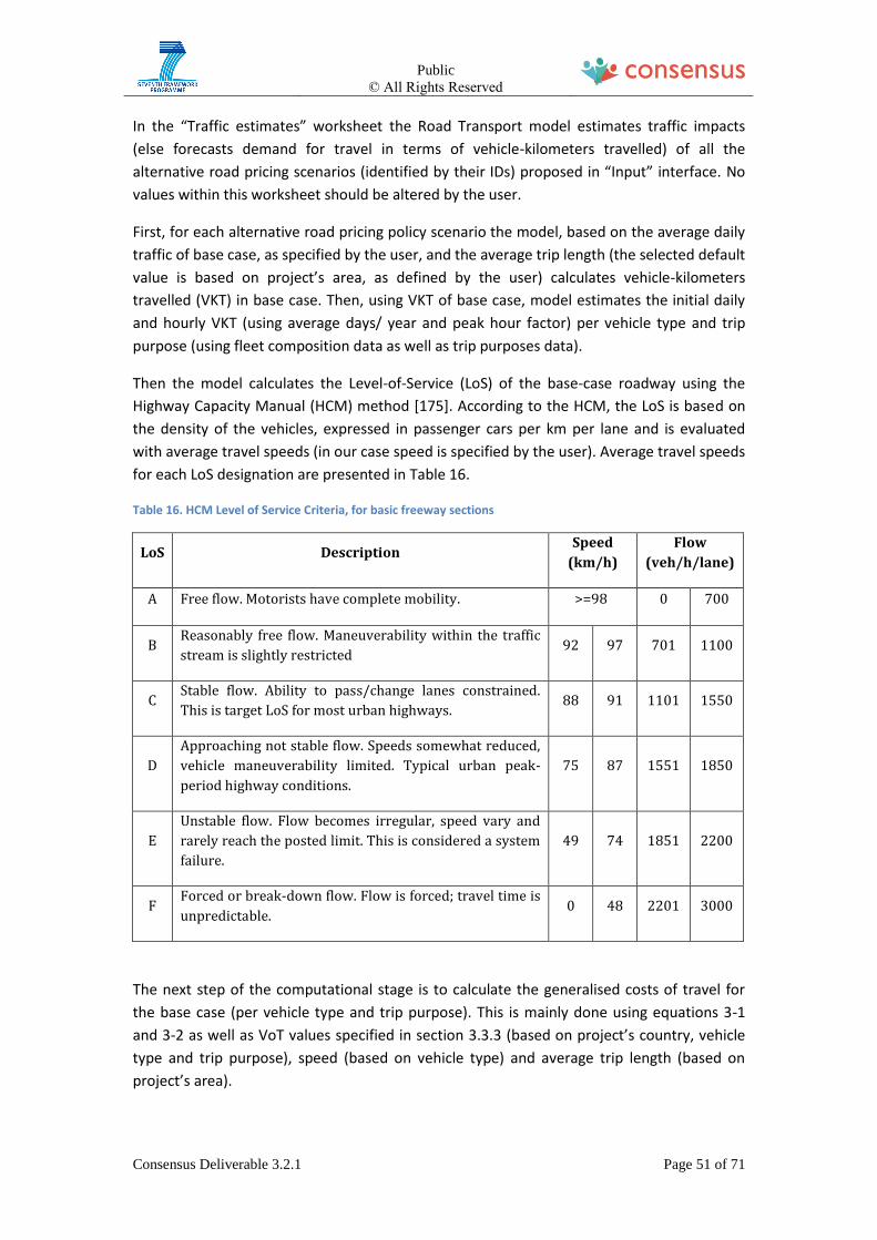
Public



In the “Traffic estimates” worksheet the Road Transport model estimates traffic impacts

(else forecasts demand for travel in terms of vehicle-kilometers travelled) of all the

alternative road pricing scenarios (identified by their IDs) proposed in “Input” interface. No

values within this worksheet should be altered by the user.

First, for each alternative road pricing policy scenario the model, based on the average daily

traffic of base case, as specified by the user, and the average trip length (the selected default

value is based on project’s area, as defined by the user) calculates vehicle-kilometers

travelled (VKT) in base case. Then, using VKT of base case, model estimates the initial daily

and hourly VKT (using average days/ year and peak hour factor) per vehicle type and trip

purpose (using fleet composition data as well as trip purposes data).

Then the model calculates the Level-of-Service (LoS) of the base-case roadway using the

Highway Capacity Manual (HCM) method [175]. According to the HCM, the LoS is based on

the density of the vehicles, expressed in passenger cars per km per lane and is evaluated

with average travel speeds (in our case speed is specified by the user). Average travel speeds

for each LoS designation are presented in Table 16.

Table 16. HCM Level of Service Criteria, for basic freeway sections

LoS Description Speed

(km/h)

Flow

(veh/h/lane)

A Free flow. Motorists have complete mobility. >=98 0 700

B Reasonably free flow. Maneuverability within the traffic

stream is slightly restricted 92 97 701 1100

C Stable flow. Ability to pass/change lanes constrained.

This is target LoS for most urban highways. 88 91 1101 1550

D

Approaching not stable flow. Speeds somewhat reduced,

vehicle maneuverability limited. Typical urban peak-

period highway conditions.

75 87 1551 1850

E

Unstable flow. Flow becomes irregular, speed vary and

rarely reach the posted limit. This is considered a system

failure.

49 74 1851 2200

F Forced or break-down flow. Flow is forced; travel time is

unpredictable. 0 48 2201 3000

The next step of the computational stage is to calculate the generalised costs of travel for

the base case (per vehicle type and trip purpose). This is mainly done using equations 3-1

and 3-2 as well as VoT values specified in section 3.3.3 (based on project’s country, vehicle

type and trip purpose), speed (based on vehicle type) and average trip length (based on

project’s area).

Public



The model then investigates how the addition of capacity, in comparison to the selected

base-case roadway, will affect traffic flows and travel speed. This is estimated using the

Index of capacity and the elasticity of demand (in VKM) with respect to capacity. This is done

using equation 3-4 presented in section 3.3.3. The additional capacity is estimated based on

lanes per direction and lane’s capacity (based on project’s area).

Once vehicle travel speed of the built scenario is estimated (using HCM method) the

generalised costs for all vehicle types and trip purposes are calculated, in each alternative

road pricing policy scenario, using equations 3-1 and 3-2. Then the ratio of old over new

generalised cost is calculated (Index), using the elasticity of demand with respect to

generalised cost (using equation 3-4).

The final stage of the “Traffic Estimates” worksheet is to compute the final daily VKT per

vehicle types for each of the alternative road pricing policy scenario examined, using

equation 3-5, specified in section 3.3.3.

Impacts Estimates

In the “Impacts estimates” worksheet the Road Transport model estimates the values of

policy objectives, that will ultimately “feed” ConsensusMOOViz tool, for the entire

alternative road pricing scenarios range, laid down in “Input” interface. Again, no values with

this worksheet should be altered by the user.

First the demand-related impacts, else policy objectives, are estimated (values in bold,

coded as C5, E5, F5, G5) using the results of “Traffic Estimates” (VKT of base case and

proposed project, per vehicle type), equations 3-6 to 3-9 as well as unit values of accidents

and external (environmental) costs included in Table 9 to Table 11, as specified in section

3.3.3.

Then the non-demand related impacts are estimated (values in bold – coded as A1, B1, H1,

I1) using the respective utility functions and Table 12 to Table 15, as specified in section

3.3.3.

It should be mentioned here that Computational Interface, calculates – in one iteration- the

traffic impacts and the policy objectives’ values, for each alternative road pricing policy

scenario, for one value of Basic Toll. Multiple iterations could be performed though, in order

to (re-)estimate traffic impacts and policy objectives’ values for various different Basic Toll

levels.

3.3.4.5 Outputs Interface

The “Outputs” interface summarizes in a simple template all policy objectives (Impacts)

values, for all alternative road pricing policy scenarios tested. The contents of this template

can be fed into the ConsensusMOOViz tool.

Public



3.3.5 Calibration and validation stages

3.3.5.1 Model validation process

To demonstrate that the model provides robust results and can be a base platform for

further option development and road pricing testing, it is necessary to show that it

realistically represents observed conditions. As the Road Transport model is generally

represented by one cordon link, it should be validated against AADT counts for the base

year, and observed average travel speed.

The standard method used to compare modeled values against observations on a link

involves the calculation of the Geoff Havers (GEH) statistic, which is an empirical form of the

Chi-squared statistic, proven extremely useful for a variety of traffic analysis.

The empirical formula for the "GEH Statistic" is:

CM

CMGEH

2*2

(Eq. 3-10)

Where M is the average daily traffic volume from the traffic model and C is the observed

average daily traffic count.

The validation of traffic counts will be subdivided in two categories:

- Validation of traffic flows

- Validation of journey times to reflect the actual base case network conditions, in terms

of network speed, distance and delay-LoS. As Consensus transport model does not

contain any detailed network coding and junction design, delay-LoS will be generated by

the speed flow curves.

During the pilot application, road transport operators and/or authorities within Europe will

be asked to participate and make a pilot test using –among other tools- Consensus transport

model to assess the impact of a known capacity improvement within their operating

highway corridor and test against 2-3 already implemented road policy pricing scenarios.

3.3.5.2 Model calibration process

Following validation stage, a basic calibration process will follow and the model will be

calibrated against observed light and heavy flows.

The % share of HGV in total traffic will be checked with real observed data. An acceptable

value of GEH is 10. Values greater than 10 require corrections and improvements of the

current assumptions and estimations of socio-economic values and basic traffic flow data.

Model calibration criteria are presented in the following table.

Table 17. Model calibration criteria

Criteria and measures Guideline

Public



GEH statistic Screenline total: GEH<4 All screenlines-in our case AADT base case

Public



4 A modelling mechanism for the policy implementation

acceptability

4.1 Introduction Consensus is an ambitious project, aiming at understanding and even predicting the effects

of a policy implementation. Critical role in that plays the opinion of the people affected by

the policy. In this work package we try to model this opinion in order to understand or

predict the effects that a low or high acceptability can have on the projected results of a

policy’s objective. For example a policy that promotes less car usage can be predicted to

have great benefits for the environment but may lead in reality, due to low public

acceptability, to limited impacts. The acceptability modeling provides Consensus with an

objective measurement of the public acceptability, making any predictions about the results

of a policy implementation more confident, both in short term and long term predictions.

A specific policy in Consensus is identified by a vector of objectives. These objectives can

have numerical ratings or even distinct ratings such as “high”, “medium” or “low”. This

rating shows the priority that the policy maker assigns to each objective and thus its

importance in the application of the policy. After each objective has been rated, either

arbitrarily by the policy maker or by a smart mechanism, a policy vector with all the

objectives and their ratings is formed, uniquely identifying the policy. The aim is to extend

the set of quantified objectives available to the policy maker by adding public acceptability

as objective. This will allow the policy maker to consider the public opinion and could

potentially help to set the priorities and conclude to one policy implementation out of the

set of available ones.

In this work, the acceptability model is implemented as a public opinion sentiment detector.

Based on a set of keywords, the model responds about the sentiment of people regarding

them. This knowledge is extracted from Twitter, where people are actively posting

information, including their opinions about various matters. The user generated content in

Twitter makes it one of the most valuable pools within which one may harvest information

about public opinion. However, Twitter was selected because it was also identified as a

reasonable source for a proof of concept implementation of the acceptability model from

the end users.

In terms of technical implementation, the acceptability model is a classifier, based on

multiple machine learning and NLP methods and trained using various Twitter dataset. Its

functionality is exposed through a web service. For demonstration purposes we have

implemented a web GUI which allows the invocation of the web service. The tool is also

integrated to a Twitter crawler implemented by ATC that returns sets of Tweets related to a

set of keywords. Then the sentiment analysis mechanism calculates the aggregate sentiment

and returns it to the web GUI. The aggregate sentiment may be a negative, near-zero or

positive number that functions as the acceptability weight for an objective (which was

expressed through the keywords mentioned above). A higher rated objective in the policy

vector with negative acceptability weight affects its acceptability negatively, one with

Public



positive acceptability weight has positive effects on its acceptability and a near-zero rated

one has small to no effect to its acceptability.

4.1.1 Scientific background

Public opinion can be measured with a number of different methods. The most popular

methods are interviews and questionnaires. In interviews the number of research subjects is

greatly limited due the need of direct interaction with the researchers. Thus, the

generalization of the results of such a study is very difficult and often erroneous [201]. On

the other hand, the questionnaires can provide the researchers with a subject pool of

adequate amount but they require great amounts of time to be distributed and analyzed. A

public acceptability tool regarding specific policies requires a real time approach.

Nowadays, we have the social media, blogs [202], tweets [203], youtube [204] and a number

of websites that encourage people to post their opinions. All this information is publically

available on the internet and it is provided in near real time delays. Researchers can use the

posts of the last two or three days and create a model of the current public opinion, without

even asking the population about it. The challenge here is the huge amount of data

available. How can the researchers pick a subset that represents the general population?

How big does this subset have to be? Which is the right tradeoff between research time and

model accuracy? Is there a way to analyze more opinions in less time?

The answer to all these challenges is the automation of the analysis. If researchers don’t

need to analyze each piece of textual data by hand, they could just use the results of the

analysis and come to valid conclusions. For this purpose an automated analysis algorithm

needs to be created. An algorithm that can understand if an opinion mediated through

textual data is positive, neutral or negative towards its subject. The challenge is that

machines are having difficulties understanding the natural language and extracting emotions

or opinions from free textual data. Therefore, the research begins for a method to transform

this opinion into something the machines can understand, numbers.

The analysis algorithms can be split into two parts: natural language processing and opinion

mining. During natural language processing (NLP) the researchers try to convert the

freeform text into numerical vectors or symbolical characters that a machine can process

more easily. The most common methods are the Bag of Words and N-Grams [205] but in the

Consensus project N-Gram Graphs are also used. Other techniques involve analysis on

sentence or even period level [206]. For the purposes of acceptability modeling the words or

N-Grams are converted into numbers showing their acceptance level. A low number could

mean that the author will not accept the policy; a medium number could mean that the

author is indifferent and a high number could mean that the author is very accepting to the

policy.

To objectively represent these “low”, “medium” and “high” thresholds machine learning is

usually employed. Using supervised or semi-supervised machine learning techniques, the

researchers train the algorithms. This training provides them with thresholds that separate

the numerical representation of the textual data into three distinct categories: no

acceptability, indifference or high acceptability. To measure the acceptability a similar term

Public



is used, i.e. the sentiment [207]. Negative emotions like hatred, dissatisfaction, unhappiness,

anger and more are connected to negative sentiments and show no acceptability for the

subject of the text. On the contrary positive emotions, like love, happiness, satisfaction,

enjoyment, are correlated to positive sentiment and high acceptability towards the subject.

4.2 Model description

4.2.1 Experiments and results

During the experimentation phase of the development a dataset of 4.451 tweets was used.

The distribution of these tweets was favoring the negative sentiments, having 1.203 tweets

of positive sentiment, 1.313 of neutral sentiment and 1.935 of negative sentiment. In order

to disassociate the results from the quality and size of the dataset as much as possible, a 10-

fold cross validation method was used to calculate the accuracy of each experiment. The

subject and thus the vocabulary of the tweets used varied greatly, providing the machine

learning algorithms with a wide set of words and characters. In order to improve their

efficiency, the textual data were cleansed by removing special characters like ‘#’ and ‘*’.

Then all characters were transformed to lowercase, all links were replaced by the keyword

‘URL’ and all references to other users were replaced by the word ‘REF’. For example the

tweet “@Elli Expert settles for biofuel *Says it is efficient, ecofriendly -...

http://t.co/aW14eUJJFH” was converted to “REF expert settles for biofuel says it is efficient,

ecofriendly -... URL”.

The only measure of comparison between each technique used was their confidence rate,

which in our case is the percentage of successful and correct categorizations. Each

experiment used a Natural Language Processing (NLP) method and a machine learning

algorithm. In total four NLP methods and seven machine learning algorithms were used

providing the researchers with a combination of 28 basic sentiment analysis algorithms. Due

to the low precision of one of the NLP methods, the combinations actually implemented

were 21. This is better explained in the following paragraphs. By fiddling with the NLP and

machine learning parameters and combining some of the basic algorithms into more

advanced ones, these 21 basic algorithms were multiplied, leading the researchers to a

number of over 200 experiments.

The NLP methods used were the Bag of Words, N-Grams, N-Gram Graphs and Triple N-Gram

Graphs. Bag of Words splits the textual data into a set of words with no consideration to

their order or contextual meaning. N-Grams split the data into pseudowords of a fixed

length of N characters again with no consideration to their order or contextual meaning. The

N-Gram Graphs split again the textual data into pseudowords of a fixed length of N

characters but this time they create a graph in which each node is a pseudoword and each

edge shows a neighboring relation between these pseudowords. The Triple N-Gram Graphs

creates a similar neighboring graph, this time though it connects both the right and left

neighbor of each pseudoword in a sentence, thus connecting triplets instead of pairs of

pseudowords.

The machine learning algorithms used were Support Vector Machine, Naïve Bayesian

Networks, Logistic Regression, Multilayer Perceptrons, Best-First Trees, Functional Trees and

Public



C4.5. Support Vector Machine and Logistic Regression try to create a mathematical function

correlating each textual input to one of the three sentiment categories; positive, neutral or

negative. The Naïve Bayesian Networks, Best-First Trees, Functional Trees and C4.5

algorithms try to create a categorization tree in which each path represents a textual input

and each leaf a successful categorization of this input into one of the three sentiment

categories. Lastly the Multilayer Perceptrons create a neural network in which many layers

of “neural nodes” process the textual input, deciding which path it should follow next until it

reaches its final destination which would be one of the three sentiment categories.

Due to the nature of the tweets and the internet slang used in them, the Bag of Words

algorithms failed to provide the researchers with acceptable confidence ratios. Moving on to

N-Gram algorithms, it was proven that a balancing the dataset, reducing the number to

3.609 evenly distributed between the three categories, and increasing the length of the

pseudo-words had higher confidence ratios. The most successful machine learning algorithm

in this case was logistic regression. Thus the best results for each different pseudo-words

lengths tried are as follows:

52.19% on 3-Grams. 65.21% on 4-Grams. 75.88% on 5-Grams.

Moving on to N-Gram Graphs, the researchers encountered even higher confidence ratios.

Except of the pseudo-words length, now they could also adjust the pruning threshold of the

graph, limiting the amount of nodes and edges available and speeding up the analysis. The

experiments show that as the threshold is approaching zero, the confidence ratios approach

100% but the processing time and space needed to store the graph is increasing rapidly.

Thus, the best results using 4-Gram Graphs reached 67.12% confidence using a threshold of

0.01 and logistic regression and a confidence of 94.53% using a threshold of 0.001 and

multilayer perceptrons. The Triple N-Gram Graphs had very similar results.

4.2.2 Component architecture

The component is based on J2EE technology and thus provides two architecture options; a

web service architecture and a java application architecture.

In the first option, all the processing is assigned to a web server, capable of handling restful

web services, such as Tomcat or Glassfish. Each interface consists of a restful web service. A

detailed list of the services is listed on a following section. The user is able to access each

interface with a web browser or an application developed in any programming language and

platform supporting restful web services, with no need for processing power because the

modeling is conducted in the backend, inside the web server.

The second option produces a java library that enables developers to include all the

modeling functionality of the component in their projects. The interface is done through

public methods that provide the same functionality as the web services discussed in the

previous paragraph. The limitation here is that the user has to be a developer and he has to

use java in order to include and call the methods provided.

Public



In either case the component uses the modeling mechanism and a training dataset. On a

second level of detail the modeling mechanism consists of a data cleansing component,

three natural language processing methods and seven machine learning algorithms. All

these components are connected to a central controller that manages their inputs and

combine their results in order to best serve each interface call.

Figure 15. Acceptability model architecture.

4.2.3 Future plans

One of the main problems encountered during the analysis is the comprising of the correct

dataset. So one of the most important goals for the future is the development of a topic

analysis mechanism in order to identify and collect more accurately tweets relevant to each

objective of a policy vector. This way the researchers would only have to enter a keyword or

a subject and the component would find relevant tweets on the internet, with the precision

of a manually collected dataset but in much greater volumes.

The amount of individual parts that comprises the modeling mechanism enables the

researchers to fiddle with a huge number of parameters, from the NLP methods used up to

the machine learning algorithms and the combination of the results. This ability provides

them with many optimization choices that require a great number of experiments. So

another important future plan is the optimization of every part in the acceptability modeling

component.

Finally a crowdsourcing part will be added to the component in order to improve the model

accuracy. This part will engage the users more actively instead of the passive approach that

sentiment analysis already provides. It’s specification are not yet decided but due to its

crowdsourcing nature it will engage a wide audience in the active research procedure, either

by requesting their contribution directly or masking it behind another “more fun action”

Public



making them not completely conscious about the effects of their actions and the true

purpose behind each decision they are required to make.

4.3 Prototype application

4.3.1 Requirements

The software is based on a Java Enterprise Edition and thus need a webserver capable of

handling Jsp pages and java based web services, such as a Glassfish or Tomcat server. The

exact specifications of this server can be greatly affected by the amount of training data

available so an exact estimation is not possible at this point. The minimum requirements

would be 2 Gigabytes of Ram, 500 Megabytes of hard disk drive and a dual core processor at

1.6 Gigahertz. Greater specifications lead to a more powerful model.

The client, or frontend, side of the software can just call web services so all that is needed is

a web connection and a web browser. More advanced tools can be built that use these

services into applications but they are not necessary for the modeling software. Due to the

fact that all of the processing is done in the server, the client does not need any processing

power.

4.3.2 Installation and deployment

The whole software can be packed into a WAR file and then deployed remotely into the

webserver, using the built-in systems such servers have. The only option that researchers

have to manually configure is the location of the training data files. These files can be

uploaded on the server or even accessed remotely by the software but in either case it

needs to be configured with the files’ URI or path.

4.3.3 Usage

All uses of the modeling software are served by web services. There are web services for

administrative usage and web services for the actual analysis. Following is a detailed list of

the available web services, their usage and the parameters they require.

Prepare (Path: prepare, Parameters: username, password); it is the service that prepares the

component for use. It should be run once every time the component is deployed or the

training dataset is changed. The preparation first creates and then trains the java objects

required for every analysis, which thereafter are kept in the server’s memory in order to

reduce the required time for analysis. The default username is “Admin” and the default

password is “AdminPass”.

Checkstatus (Path: checkstatus, Parameters: clientid, mode); it is a mainly internal web

service, used to check the status of an ongoing analysis and avoid web timeout errors. It

requires the ‘id’ of the running procedure to be checked and the ‘mode’ which can be either

prepare (for the preparation procedures of the model), pie (for the pie chart analysis or any

other word or number for a normal analysis. It returns a confirmation that the process is still

running or the result if it has already been completed.

Public



Result (Path: result, Parameters: id, clientid); it is an internal and public web service that

checks if the results of an analysis are in the system and if they are it returns them to the

caller in the form of an XML document. As parameters it needs the ‘id’ of the analysis.

PieResult (Path: pieResult, Parameters: id, clientid); it is an internal and public web service

that checks if the results of an analysis are in the system and if they are it returns them to

the caller in the form of a pie chart. As parameters it needs the ‘id’ of the analysis.

AnalyzeId (Path: analyseid, Parameters: id); it is the main analysis service. As parameters it

requires the id of a tweet to be analyzed. The result is an XML file that contains the

numerical results of the analysis using each available algorithm. These values show the

possibility that the analyzed tweet is categorized as a tweet of positive, neutral or negative

sentiment.

Pie (Path: pie, Parameters: id, method); it is a visual analysis service. As parameters it

requires the id of a tweet to be analyzed. The result is an HTML file that contains a pie chart

with the results of the analysis using each available algorithm. These values show the

possibility that the analyzed tweet is categorized as a tweet of positive, neutral or negative

sentiment.

Test (Path: test, Parameters: id, method); it is a singular algorithm analysis service. As

parameters it requires the id of a tweet to be analyzed and the keyword of an algorithm, if

the algorithm is not specified then the default algorithm is used. The result is an XML file

that contains the numerical results of the analysis using the specified algorithm. These

values show the possibility that the analyzed tweet is categorized as a tweet of positive,

neutral or negative sentiment.

AnalyzeSet (Path: analyzeset, Parameters: filepath); a web service to analyze a set of tweets.

As parameters it requires the full file URI (filepath and filename) to analyze. The result is a

numerical value that shows how much the public likes or dislikes the subject of this set, a

negative value would show dislike and thus a higher value in the corresponding objective of

the policy would result to negative acceptability, a near-zero value would show indifference

and does not affect the policy acceptability and a positive value would show high

acceptability and thus a higher value in the corresponding objective of the policy vector

would have positive acceptability effects.

AnalyzeKeyword (Path: analyzekeyword, Parameters: keyword); a web service much like

AnalyzeSet but in this case it requires just a keyword in order to automatically construct the

dataset. It returns the same type of values as AnalyzeSet.

The available algorithms and their keywords are as follows:

Table 18. Available algorithms and keywords.

Keyword NLP Method Machine Learning Tool

Simplesvm N-Grams Support Vector Machine

Simplebayes N-Grams Bayesian Networks

simplec45 N-Grams C4.5

Public



Simplelogistic N-Grams Logistic Regression

Simplesimplelogistic N-Grams Simple Logistic Regression

Simplemlp N-Grams MultiLayer Perceptrons

Simplebftree N-Grams Best-First Trees

Simpleft N-Grams Functional Trees

Graphsvm N-Gram Graphs Support Vector Machine

Graphbayes N-Gram Graphs Bayesian Networks

graphc45 N-Gram Graphs C4.5

Graphlogistic N-Gram Graphs Logistic Regression

Graphgraphlogistic N-Gram Graphs Simple Logistic Regression

Graphmlp N-Gram Graphs MultiLayer Perceptrons

Graphbftree N-Gram Graphs Best-First Trees

Graphft N-Gram Graphs Functional Trees

Triplegraphsvm Triple N-Gram Graphs Support Vector Machine

Triplegraphbayes Triple N-Gram Graphs Bayesian Networks

triplegraphc45 Triple N-Gram Graphs C4.5

Triplegraphlogistic Triple N-Gram Graphs Logistic Regression

triplegraphtriplegraphlogistic Triple N-Gram Graphs Simple Logistic Regression

Triplegraphmlp Triple N-Gram Graphs MultiLayer Perceptrons

Triplegraphbftree Triple N-Gram Graphs Best-First Trees

Triplegraphft Triple N-Gram Graphs Functional Trees

Simpleaverage N-Grams Combinational with Average

Rule

Simplemajority N-Grams Combinational with Majority

Rule

Simpleeuclidean N-Grams Combinational with

Euclidean Distances

Simplemanhattan N-Grams Combinational with

Manhattan Distances

Simplecosine N-Grams Combinational with Cosine

Dissimilarity

Simplechebychev N-Grams Combinational with

Chebychev Distances

Simpleorthocos N-Grams Combinational with Cos-

based Orthodromic Distances

Simpleorthosin N-Grams Combinational with Sin-


Simpleorthotan N-Grams Combinational with Tan-


Grapheaverage N-Gram Graphs Combinational with Average

Rule

Graphemajority N-Gram Graphs Combinational with Majority

Rule

Grapheuclidean N-Gram Graphs Combinational with

Euclidean Distances

Graphmanhattan N-Gram Graphs Combinational with

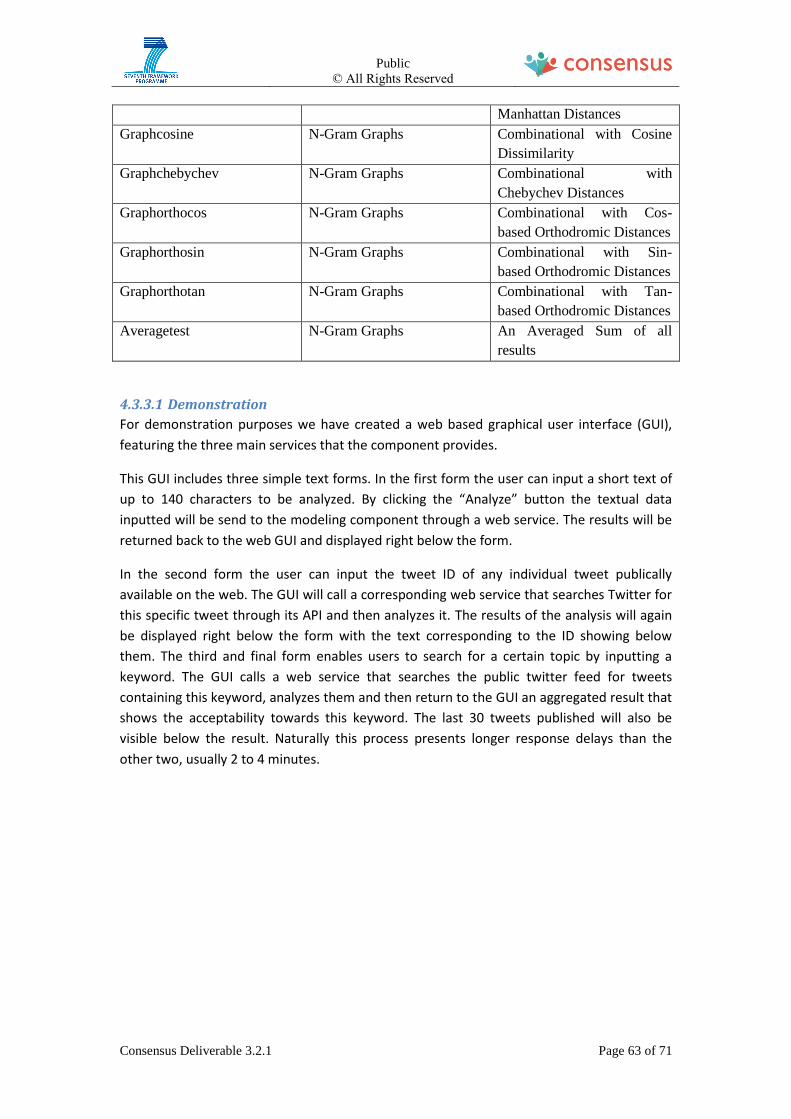
Public



Manhattan Distances

Graphcosine N-Gram Graphs Combinational with Cosine

Dissimilarity

Graphchebychev N-Gram Graphs Combinational with

Chebychev Distances

Graphorthocos N-Gram Graphs Combinational with Cos-


Graphorthosin N-Gram Graphs Combinational with Sin-


Graphorthotan N-Gram Graphs Combinational with Tan-


Averagetest N-Gram Graphs An Averaged Sum of all

results

4.3.3.1 Demonstration

For demonstration purposes we have created a web based graphical user interface (GUI),

featuring the three main services that the component provides.

This GUI includes three simple text forms. In the first form the user can input a short text of

up to 140 characters to be analyzed. By clicking the “Analyze” button the textual data

inputted will be send to the modeling component through a web service. The results will be

returned back to the web GUI and displayed right below the form.

In the second form the user can input the tweet ID of any individual tweet publically

available on the web. The GUI will call a corresponding web service that searches Twitter for

this specific tweet through its API and then analyzes it. The results of the analysis will again

be displayed right below the form with the text corresponding to the ID showing below

them. The third and final form enables users to search for a certain topic by inputting a

keyword. The GUI calls a web service that searches the public twitter feed for tweets

containing this keyword, analyzes them and then return to the GUI an aggregated result that

shows the acceptability towards this keyword. The last 30 tweets published will also be

visible below the result. Naturally this process presents longer response delays than the

other two, usually 2 to 4 minutes.

Public



5 References [1] Muhammad, A., J. Seale, B. Meade, and A. Regmi, International Evidence on Food

Consumption Patterns: An Update Using 2005 International Comparison Program Data.Technical Bulletin (1929) 2011, USDA-ERS: Washington, D.C. .

[2] Skalský, R., Z. Tarasovičová, J. Balkovič, E. Schmid, M. Fuchs, E. Moltchanova, G. Kindermann, and P. Scholtz, GEO-BENE global database for bio-physical modeling v. 1.0 - concepts, methodologies and data. The GEO-BENE database report. 2008, International Institute for Applied Systems Analysis (IIASA), Austria. p. 58.

[3] Izaurralde, R.C., J.R. Williams, W.B. McGill, N.J. Rosenberg, and M.C.Q. Jakas, Simulating soil C dynamics with EPIC: Model description and testing against long-term data. Ecological Modelling, 2006. 192(3-4): p. 362-384.

[4] Williams, J.R., The EPIC Model, in Computer Models of Watershed Hydrology, V.P. Singh, Editor. 1995, Water Resources Publications, Highlands Ranch, Colorado. p. 909-1000.

[5] Herrero, M., P. Havlík, H. Valin, A. Notenbaert, M.C. Rufino, P.K. Thornton, M. Blümmel, F. Weiss, D. Grace, and M. Obersteiner, Biomass use, production, feed efficiencies, and greenhouse gas emissions from global livestock systems. Proceedings of the National Academy of Sciences, 2013.

[6] Kindermann, G.E., M. Obersteiner, E. Rametsteiner, and I. McCallum, Predicting the deforestation-trend under different carbon-prices. Carbon Balance and Management, 2006. 1(1): p. Art. no. 15.

[7] Ruesch, A. and H.K. Gibbs, New IPCC Tier-1 Global Biomass Carbon Map For the Year 2000. 2008, Available online from the Carbon Dioxide Information Analysis Center http://cdiac.ornl.gov, Oak Ridge National Laboratory, Oak Ridge, Tennessee.

[8] Gallagher, E., The Gallagher Review of the indirect effects of biofuels production. 2008, Renewable Fuels Agency: St Leonards-on-Sea. p. 92.

[9] Lotze-Campen, H., M. von Lampe, P. Kyle, S. Fujimori, P. Havlik, H. van Meijl, T. Hasegawa, A. Popp, C. Schmitz, A. Tabeau, H. Valin, D. Willenbockel, and M. Wise, Impacts of increased bioenergy demand on global food markets: an AgMIP economic model intercomparison. Agricultural Economics, 2013: p. n/a-n/a.

[10] EC, Impact assessment - A Roadmap for moving to a competitive low carbon economy in 2050. 2011, European Commission (EC): Brussels. p. 133.

[11] Alexandratos, N. and J. Bruinsma, World Agriculture Towards 2030/2050 The 2012 Revision. 2012, FAO: Rome. p. 160.

[12] EC, Directive 2009/28/EC of the European Parliament and of the Council of 23 April 2009 on the promotion of the use of energy from renewable sources and amending and subsequently repealing Directives 2001/77/EC and 2003/30/EC T.E.P.a.C.o.t.E. Union, Editor. 2009: Brussels. p. 107

[13] EC, EU Energy, Transport and GHG Emissions Trends to 2050: Reference Scenario 2013. 2013, European Commission Directorate-General for Energy, DG Climate Action and DG Mobility and Transport.: Brussels. p. 168.

[14] Kapos, V., C. Ravilious, A. Campbell, B. Dickson, H. Gibbs, M. Hansen, I. Lysenko, L. Miles, J. Price, and J. Scharlemann, Carbon and biodiversity: a demonstration atlas. UNEP-WCMC, Cambridge, UK, 2008.

[101] Arup and Oxera (2010) How should the revised elasticity-based framework be implemented? Guidance report, Prepared for the DfT Transport Scotland and the Passenger Demand Forecasting Council [102] Auckland Regional Council (ARC). (2009). Non-Network Policy Options for the

Auckland Regional Land Transport Strategy

http://cdiac.ornl.gov/

Public



(http://www.arc.govt.nz/transport/regional-land-transport-strategy-2005/the-new-regional-land-transport-strategy.cfm)

[103] Australian Bureau of Infrastructure, Transport and Regional Economics (BITRE) (http://www.bitre.gov.au/) (visited on June 2014)

[104] Balducci, P., Shao, G., Amos, A. and Rufolo, A. (2011) Costs of Alternative Revenue-Generation Systems, NCHRP. Research sponsored by the American Association of State Highway and Transportation Officials in cooperation with the Federal Highway Administration. TRB, Washington D.C.

[105] Boulter, R. and Wignall, D. (2008) Identifying the value in long distance rail services. , published on the Victoria Transport Policy Institute website (www.vtpi.org/rail_evaluation.pdf)

[106] Bowerman, A. (2007). The Costs and Benefits of Road Pricing: Comparing Nationwide Charging with Project-Based Schemes, Institute of Economic Affairs (IEA) Discussion Paper No. 18.

[107] CE Delft, INFRAS, ISI and University of Gdansk (2008) Handbook on estimation of external costs in the transport sector, produced within the study Internalisation Measures and Policies for All external Cost of Transport (IMPACT), prepared for the European Commission, Version 1.1, Delft, CE.

[108] Center for Transportation Analysis. Analysis of Automobile Travel Demand Elasticities with Respect to Travel Cost, Oak Ridge National Laboratory managed by UT-Battelle, LLC for the U.S. Department of Energy under Contract number DE-AC05-00OR22725 (http://www-cta.ornl.gov/cta/One_Pagers/NHTS_Travel_Demand_Elasticity.pdf) (visited on June 2014).

[109] Cervero, R. and Hansen, M. (2000). Road Supply-Demand Relationships: Sorting Out Casual Linkages, Institute of Transportation Studies, University of California (www.uctc.net).

[110] Conference of European Directors of Roads, Project Group Funding. (2009). The socio-economic impacts of Road Pricing. CEDR Secretariat General.

[111] CURACAO. (2009a). Deliverable D2: State of the Art Review. Project: Coordination of Urban Road User Charging Organisational Issues Sponsored by European Commission under the FP6 Framework

[112] CURACAO. (2009b). Deliverable D3: Case Study results. Project: Coordination of Urban Road User Charging Organisational Issues Sponsored by European Commission under the FP6 Framework.

[113] Danna, S., Mori, K., Vela, J. and Ward, M. (2012). A Benefit-Cost Analysis of Road Pricing in Downtown Seattle, Evans School Review, Vol. 2, No. 1.

[114] De Borger, B. and Wouters, S. (1998). Transport externalities and optimal pricing and supply decisions in urban transportation: a simulation analysis for Belgium, Regional Science and Urban Economics, vol.28, no.2, pp.163-197

[115] De Corla-Souza, P. (1998). Using SPASM for Transportation Decision-Making. United States Department of Transportation - Federal Highway Administration (https://www.fhwa.dot.gov/steam/spasm.htm)

[116] De Corla-Souza, P. and Cohen, H (1999). Accounting for induced travel in evaluation of urban highway expansion. United States Department of Transportation - Federal Highway Administration (https://www.fhwa.dot.gov/steam/doc.htm)

[117] De Corla-Souza, P. (2002). Evaluation of Toll Options Using Quick-Response Analysis Tools: A Case Study of the Capital Beltway. United States Department of Transportation - Federal Highway Administration (http://www.fhwa.dot.gov/steam/smitemldoc.htm)

Public



[118] De Jong, G.C., Tegge, O., Dohmen, R., Ettema, D.F., Hamer, R.N., Massiani, J. and van Vuren, T. (1998). Review of existing evidence on time and cost elasticities of travel demand and on value of travel time (Deliverable 1) TRACE Costs of private road travel and their effects on demand, including short and long term elasticities, European Commission Directorate-General for Transport.

[119] Dehghani, Y. and Olsen, W. (1998). Potential Pitfalls in Forecasting Travel Demand for Toll Roads: Experience in the US and Overseas. Transportation Research Board Annual Meeting - November 1998, Paper 99051.

[120] Department for Transport (2001) Transport Economics Note (TEN), London. [121] Department for Transport (2004) Transport of Goods by Road in Great Britain 2003.

Transport Statistics Bulletin, London. [122] Department for Transport (2009a) Webtag units: 1.1 Analysis; 2.1 Approach; 2.4

Summary on modelling; 2.9.1 Variable demand modelling: 3.1 Modelling detail (http://www.dft.gov.uk/webtag)

[123] Department for Transport. (2009b). National Transport Model (http://www.dft.gov.uk/pgr/economics/ntm/)\

[124] Downs, A. (2007). Still Stuck in Traffic: Coping with Peak-Hour Traffic. Washington, D.C.: Brookings Institute Press.

[125] Eenink, R.G., Dijkstra, A., Wijnen, W. and Janssen, S.T.M.C. (2007). Road pricing and road safety; Possible effects on road safety of 23 variants of road pricing. SWOV. R-2007-4N.

[126] Eliasson, J. (2008). Cost-Benefit Analysis of the Stockholm Congestion Charging System. Centre for Transport Studies, Royal Institute of Technology.

[127] Elvik, R. and Vaa, T. eds (2004). The Handbook of road safety measures. Elsevier. [128] Ensor, J. (2005) Multi-Criteria Analysis: An Alternative Approach for the Evaluation of

Road Pricing Strategies. Submitted to the Department of Civil and Environmental Engineering in Partial Fulfillment of the Requirements for the Degree of Master of Science in Transportation at the Massachusetts Institute of Technology.

[129] Fleming, D.S. (2012) Dispelling the Myths: Toll and Fuel Tax Collection Costs in the 21st Century. Policy Study 409, Reason Foundation.

[130] Friedman, D. and Waldfogel, J. (1994) The administrative and compliance cost of manual higway toll collection: evidence from Massachusetts and New Jersey. National Tax Journal, Vol. 47, No.2, pp. 217-28.

[131] Furnish, P. and Wignall, D. (2009). Making the Most of Models: Using Models To Develop More Effective Transport Policies And Strategies, Reviewed from Willumsen, L. (Steer Davies Gleave), published on the Victoria Transport Policy Institute website (http://www.vtpi.org/FerWig_Modelling.pdf)

[132] Greene, D.L. (1992). Vehicle use and fuel economy: How big is the "rebound" effect? The Energy Journal, vol.13, no.1, pp. 117-143

[133] Gunn, H.F., Tuinenga, J.G., Allouche, J.F. and Debrincat, L. (1998) ANTONIN: A forecasting model for travel demand in the Ile de France, Transport Planning Methods, Volume II, European Transport Conference, Proceedings of Seminar E, vol. P424, pp.99-121.

[134] Hansen, M. and Huang, Y. (1997). Road Supply and Traffic in California Urban Areas, Transportation Research A, Vol. 31, No. 3, pp. 205-218.

[135] HDR (2009) Comparing Administrative Costs of Collecting Highway Revenues: Fuel Tax vs. Direct User Charge, prepared for the Office of Economic and Strategic Analysis, U.S. Department of Transportation.

[136] HEATCO (2006) Deliverable 5: Proposal for Harmonised Guidelines. Project: Developing Harmonised European Approaches for Transport Costing and Project Assessment, prepared for the European Commission.

Public



[137] Hensher, D. and Button, K.J. (2007). Handbook of transport modelling: 2nd edition, Handbooks in Transport - VOLUME 1, Emerald Group Publishing Ltd.

[138] Hyman, G.M. and Wilson, A.G. (1968). The effects of changes in travel costs on trip distribution and modal split. Centre for Environmental Studies, Working paper 21.

[139] IBI Group (2007) Comparative Analysis of Toll Facility Operational Costs, Report for the Washington State Department of Transportation

[140] Intergovernmental Panel for Climate Change (IPCC). (2007). Climate change 2007: the physical science basis: summary for policymakers. IPCC Secretariat.

[141] Jaako Poyry Infra, HB-Verkehrsconsult. (2004). State of the Art Analysis of European Toll Collection Systems. IBTTA Fall Technology Workshop, November 13-16, Madrid, SPAIN

[142] Jones, P. (1995). Road Pricing: The Public Viewpoint. In B. Johannson and L.-G. Mattsson (Eds.), Road Pricing: Theory, Empirical Assessment and Policy. Boston, Dordrecht, London: Kluwer Academic Publishers, 159-180.

[143] Jones, P. (1998). Urban Road Pricing: Public Acceptability and Barriers to Implementation. In K. J. Button and E. T. Verhoef (Eds.), Road Pricing, Traffic Congestion and the Environment. Cheltenham: Edward Elgar, 263-284.

[144] JV SDG-NAMA-SALFO (2003) Provision of Services of Specialized Traffic Advisor for Motorway Concession Contracts in Greece: Data Processing and Traffic Model Development, prepared for the Hellenic Ministry of Environment, Physical Planning and Public Works.

[145] Khisty, C.J. and Sriraj, P.S. (1996) Use of Scenario-Building Transportation Model for Developing Countries. Transportation Research Board. Transportation Research Record Vol. 1563 (1996), pp. 16-25.

[146] KonSULT- the Knowledgebase on Sustainable Urban Land use and Transport. Road User Charging.http://www.konsult.leeds.ac.uk/private/level2/instruments/instrument001/l2_001b.htm (visited on January 2014)

[147] Kriger, D. (2005). Traffic and Revenue Forecasting for Roads and Highways Concerns, Methods and a Checklist for Practioners. Proceedings of the Expert Forum on Road Pricing and Travel Demand Modeling, November 14-15, Hilton Alexandria Old Town. Sponsored the Office of Transportation Policy/U.S. Department of Transportation.

[148] Komanoff, C. (1997). Environmental Consequences of Road Pricing: A Scoping Paper for The Energy Foundation. Komanoff Energy Associates, New York (NY).

[149] Lesley, L. (2009) Generalised Costs and the Value of Time as a Method of Patronage Forecasting. Acta Technica Jaurinensis, Vol.2, No.1, pg. 57-68.

[150] Litman, T. (2013). Well Measured: Developing Indicators for Sustainable and Livable Transport Planning. Victoria Transport Policy Institute.

[151] Litman, T. (2014) Generated Traffic and Induced Travel. Victoria Transport Policy Institute.

[152] Matas, A and Raymond, J.L. (2003). Demand Elasticity on Tolled Motorways. Journal of Transportation and Statistics Volume 6, no. 23, Bureau of Transport Statistics Publications.

[153] National Road Transport Commission and National Transport Secretariat (2003) Candidate Actions to Progress Road Pricing Initiatives. Report Prepared by: Maunsell Australia Pty Ltd and MM Starrs Pty Ltd.

[154] Noland, R.B. and Lem, L.L. (2002). A Review of the Evidence for Induced Travel and Changes in Transportation and Environmental Policy in the US and the UK, Transportation Research D, Vol. 7, No. 1, pp. 1-26.

[155] Omann, I. (2004) Multi-criteria decision aid as an approach for sustainable development analysis and implementation. Dissertation submitted to obtain the

Public



Academic Degree of a Doctor of Social and Economic Sciences at the Karl-Franzens University of Graz.

[156] Ortuzar, J. (1992) Simplified Transport Demand Modelling (PTRC perspectives series). PTRC Education and Research Services.

[157] Ortuzar, J. and Willumsen, L. (2006). Modelling Transport: 3rd edition. Wiley. [158] PBS&J (2009) WSDOT Statewide Tolls Program: Toll Operations Benchmarks and

Incentives, prepared for the Washington State Department of Transportation (WSDOT).

[159] PIARC (2008). Pricing as a tool for funding and regulation with equity in mind. Committee TC 1.1, Road system economics Working Group report.

[160] Pigou, A. C. (1920). The Economics of Welfare. London: Macmillan [161] Poriotis, N. and Vakirtzidis N. (2001). Study on Vehicle Operating Costs Estimation,

prepared for the Directorate of Road Construction Works Studies/Research, Hellenic Ministry of the Environment, Physical Planning and Public Works.

[162] PROSPECTS. (2003). Deliverable 14: Delivering Sustainable Land Use and Transport Strategies, A Methodological Guidebook. Project: Procedures for Recommending Optimal Sustainable Planning of European City Transport Systems, sponsored by European Commission under the 5th Framework - EESD.

[163] Rothengatter, W. and Doll, C. (2001). Anforderungen an eine umweltorientierte Schwerverkehrsabgabe. Texte des Umweltbundesamtes Nr. 71/01, Berlin.

[164] Santos, G. (2000). On the Economic, Technological and Political Aspects of Road Pricing as a Tool for Traffic Demand Management. Proceedings of the European Transport Conference, 11th -13th September 2000, Homerton College, Cambridge.

[165] Santos G. and Shaffer, B. (2004). Preliminary Results of the London Congestion Charging Scheme, presented at the 83rd Annual Meeting of the Transportation Research Board, Washington DC, 11-15 January 2004.

[166] Schnier, J. (1999). Stadtvignetten als Steuerungsinstrument im Straßenverkehr – Beurteilung und Wirkungsprognose am Beispiel der Stadt Köln; Bielefeld: Erich Schmidt.

[167] Small, K. A., Gomez-Ibañez, J.A. (1998). Road Pricing for Congestion Management: The Transition from Theory to Policy. The University of California, Transportation Center. University of California at Berkeley. pg. 213.

[168] Small, K. and Winston, C. (1999). The Demand for Transportation: Models and Applications, in Essays in Transportation Economics and Policy, Brookings Institute (www.brooking.edu).

[169] Smith, D., Chang-Albitres, C., Stockton, W. and Smith, C. (2004). Estimating Revenues Using a Toll Viability Screening Toll, Report FHWA/TX-050/0-4726-1 prepared for the Federal Highways Administration, Texas Transportation Institute, College Station, Texas.

[170] Spear, B. (2005). A Summary of the Current State of the Practice In Modeling Road Pricing. Proceedings of the Expert Forum on Road Pricing and Travel Demand Modeling, November 14-15, Hilton Alexandria Old Town. Sponsored the Office of Transportation Policy/U.S. Department of Transportation.

[171] Teubel, U. (2001). Road Pricing - effizient aber unsozial?. Europäische Hochschulschriften Reihe 5. Bern: Peter Lang Verlag.

[172] TDM Encyclopedia (2014) Transport Model Improvements: Improving Methods for Evaluating The Effects and Value of Transportation System Changes, published on the Victoria Transport Policy Institute website (http://www.vtpi.org/tdm/tdm125.htm)

[173] Transport for London. (2004). Impacts Monitoring – Second Annual Report; April 2004, London.

Public



[174] Transportation Research Board (1980). The vehicle-miles of travel - urban highway supply relationship. National Cooperative Highway Research Program Research Results Digest, no. 127, pp.1-7

[175] Transportation Research Board (1994) The Highway Capacity Manual (HCM). Washington DC.

[176] Troyer, S. (2002). Verteilungswirkungen der Mauten im Alpenraum; Diplomarbeit an der Leopold-Franzens-Universität Innsbruck (in Kooperation mit der ETH Zürich)

[177] Tsamboulas, D. and Kopsacheili, A. (2003). A Methodological Framework for the Strategic Assessment of Transportation Policies: Application for the Athens 2004 Olympic Games. Transportation Research Board. Transportation Research Record Vol. 1848 (2003), pp.19-28.

[178] United Nations (2003) Cost Benefit Analysis of Transport Infrastructure projects - TINA Appraisal Guidance.

[179] Urban Analytics Inc. and URS Corporation. (2004). Estimating Demand for Value Pricing Projects – State of the Practice, Final Draft. Prepared for the North Central Texas Council of Governments.

[180] U.S. Department of Transportation (1999) Participant Notebook for NHI Course No. 15260, Advanced Travel Demand Forecasting Course. Publication No. FHWA-HI-99-003. Washington, DC.

[181] U.S. Department of Transportation (2008). TRUCE 3.0 User’s Guide (http://www.fhwa.dot.gov/ipd/revenue/road_pricing/tools/).

[182] U.S. Department of Transportation (2009) TRUCE-ST User’s Guide (http://www.fhwa.dot.gov/ipd/revenue/road_pricing/tools/).

[183] U.S. Department of Transportation - Research and Innovative Technology Administration (RITA) - (http://www.itscosts.its.dot.gov/ITS/benecost.nsf/ID/CD91641C96A0DE1985257B6A004DF1D6?OpenDocument&Query=CApp) (visited on May 2014)

[184] Van Wee, B. (2011). Transport and Ethics: Ethics and the Evaluation of Transport Policies and Projects. Edward Elgar Publishing.

[185] Verhoef, E., Bliemer, M., Steg, L., van Wee, B. (2008). Pricing In Road Transport, A Multi-Disciplinary Perspective. Edward Elgar Publishing.

[186] Victoria Transport Policy Institute (2013). Transport Demand Management Encyclopedia - Road Pricing. http://www.vtpi.org/tdm/tdm35.htm

[187] Vovsha, P., Davidson, W., Donnelly, R. (2005). Making the State of the Art the State of the Practice Advanced Modeling Techniques for Road Pricing. Proceedings of the Expert Forum on Road Pricing and Travel Demand Modeling, November 14-15, Hilton Alexandria Old Town. Sponsored the Office of Transportation Policy/U.S. Department of Transportation.

[188] Walker, J. (2011). The acceptability of Road Pricing. Copyright Royal Automobile Club Foundation for Motoring Ltd.

[189] Wignall, D. (2008). Big picture transport planning: When precision fails and approximation succeeds. 43rd Operational Research Society of NZ Conference, Victoria University, December 2008.

[190] Winston, C. (1985). Conceptual developments in the economics of transportation: An interpretive survey, Journal of Economic Literature, vol.23, no.1, pp.57-94.

[191] Winter, M. and Hirschhausen, C. von. (2005). Multi Functional Urban HDV Road Pricing – An Empirical Analysis of Berlin. Final Report TELLUS WP 6.5.2, Berlin.

[192] Zahavi, Y. (1981). A new urban travel modeling, in Global Modelling: Lecture Notes in Control and Information Sciences, Volume 35, pp.130-138. Springer.

[193] Zerbe, R.O. Jr and Dively, D. (1994). Benefit-Cost Analysis: In Theory and Practice, HaperCollin Paper Publisher: 139-142, 290.

Public



[201] Payne, G., Williams, M., 2005. Generalization in Qualitative Research. Sociology 39, 295–314. doi:10.1177/0038038505050540

[202] Godbole, N., Srinivasaiah, M., Skiena, S., 2007. Large-Scale Sentiment Analysis for News and Blogs, in: Proceedings of the International Conference on Weblogs and Social Media (ICWSM).

[203] Bifet, A., Frank, E., 2010. Sentiment Knowledge Discovery in Twitter Streaming Data., in: Pfahringer, B., Holmes, G., Hoffmann, A.G. (Eds.), Discovery Science, Lecture Notes in Computer Science. Springer, pp. 1–15.

[204] Morency, L.-P., Mihalcea, R., Doshi, P., 2011. Towards multimodal sentiment analysis: harvesting opinions from the web., in: Bourlard, H., Huang, T.S., Vidal, E., Gatica-Perez, D., Morency, L.-P., Sebe, N. (Eds.), ICMI. ACM, pp. 169–176.

[205] Aisopos, F., 0001, G.P., Tserpes, K., Varvarigou, T.A., 2012. Content vs. context for sentiment analysis: a comparative analysis over microblogs., in: Munson, E.V., Strohmaier, M. (Eds.), HT. ACM, pp. 187–196.

[206] Wilson, T., Wiebe, J., Hoffmann, P., 2005. Recognizing Contextual Polarity in Phrase-Level Sentiment Analysis, in: hltemnlp2005. Vancouver, Canada, pp. 347–354.

[207] Pang, B., Lee, L., 2008. Opinion mining and sentiment analysis. Found. Trends Inf. Retr. 2, 1–135.

d3.2.1 models and simulators report - cordis · doc ref: deliverable 3.2.1 ... land use model which...

Documents