d1.1 profile and needs of cmc - esa climate office

Document Ref.: D1.1: Profile and main needs of the climate modelling community CMUG Deliverable Number: D1.1 Due date: August 2010 Submission date: 31 August 2010 Version: 1.0

1

Climate Modelling User Group Deliverable 1.1 Profile and main needs of the climate modelling community Centres providing input: MOHC, MPI-M, ECMWF, MétéoFrance

Version nr. Date Status 1.0 31 August 2010 Final draft to ESA


2

Deliverable 1.1 Profile and main needs of the climate modelling community Contents 1. Overview 2. Breakdown and profile of the climate modelling community 3. List of key experts 4. European climate models 5. Satellite Data Needs of Climate Modelling Centres

5.1. Introduction

5.2 Generic requirements for satellite datasets

5.3. ECVs required for climate applications

6. Glossary

7. Results of the CMUG Questionnaire


3

1. Overview This document provides an overview of how the Climate Modelling User Group collected information about requirements which is not only relevant to the initial 11 ECVs selected by ESA but for all of the GCOS ECVs which can be measured from satellites. In section 2 there is a profile of the climate modelling community listing the main activities which are underway and might be linked to the CCI projects and which partners in the CMUG are involved in each activity. In section 3 is the mailing list of key experts in both global and regional modelling which was used to solicit inputs to the requirement gathering. In section 4 is a summary of the European climate models. In section 5 is a description of the data needs of climate modelling centres. A glossary of terms is provided in section 6. Finally, section 7 gives a summary of the output from the on-line questionnaire and also includes comments from the workshop held in Vienna in May 2010.


4

2. Profile of the climate modelling community The table below gives the list of climate model related activities which are relevant to the ESA CCI project. CMUG partners with direct involvement in each activity are indicated by a cross in the table. This list is evolving all the time. Project Link MOHC ECMWF MPI MF

Satellite and in situ data projects GCOS www.wmo.int/pages/prog/g

cos/index.php X X X X

GSICS www.star.nesdis.noaa.gov/smcd/spb/calibration/icvs/GSICS/

X

Climate SAF http://www.cmsaf.eu X

NWP SAF http://nwpsaf.org X X X

EG-CLIMET http://www.eg-climet.org/ X X

Atmosphere IPCC www.ipcc.ch X X X X

CFMIP www.cfmip.net X X X

CMIP5 X X X X COSP cfmip.metoffice.com/COSP

.html X X X X

QuARL/JADE (EarthCare)

X X X X

GERB SG www.sstd.rl.ac.uk/gerb/ X

GRAS SAG/SAF www.grassaf.org X X

IASI Science smsc.cnes.fr/IASI/A_doc_isswg.htm

X X X

GEWEX projects www.gewex.org/projects.html

X X X X

GlobVAPOUR X EUCAARI www.atm.helsinki.fi/eucaari X X X

AEROCOM nansen.ipsl.jussieu.fr/AEROCOM/objectives.html

X X

GlobAEROSOL http://www.globaerosol.info/

X

MACC/GEMS gems.ecmwf.int X X

GEWEX CEOP monsoon.t.u-tokyo.ac.jp/ceop2/index.html

X

Ocean MyOcean www.myocean.eu.org X X

GHRSST www.ghrsst.org X X

ARC arc.geos.ed.ac.uk X


5

AATSR SAG www.leos.le.ac.uk/aatsr X X

GODAE OceanView

www.godae.org/oceanview.html

X X

Damocles www.damocles-eu.org X

Ice2sea http://www.ice2sea.eu/ X

NEMO www.nemo-ocean.eu X X

Land ECEarth ecearth.knmi.nl X

JULES www.jchmr.org/jules/ X

TERRABITES www.terrabites.net X

GlobALBEDO X High Noon www.eu-highnoon.org X

CarboEurope www.carboeurope.org X X

CARBONES X X Reanalyses

ERA-40/ERA-Interim/ERA-CLIM

www.ecmwf.int/research/era/do/get/index

X X X X

EURO4M www.euro4m.eu X X X

JRA-25 http://www.jreap.org/indexe.html

NCEP Reanalysis http://www.esrl.noaa.gov/psd/data/reanalysis/reanalysis.shtml

Climate modelling and impacts WATCH www.eu-watch.org X

COMBINE www.combine-project.eu X X

EUCLIPSE X X X X ENSEMBLES www.ensembles-eu.org X X X X

QUANTIFY www.pa.op.dlr.de/quantify X

Technical projects for climate modelling ENES www.enes.org X X X

METAFOR metaforclimate.eu X X


6

3. List of key experts Note: Institutes and experts in CMUG are not given in these lists. Global Model Experts Country Centre Model Point-of-contact US GFDL GFDL Leo Donner GISS GISS Gavin Schmidt NCAR CCSM Jim Hurrell JPL Joao Teixeira NASA/GMAO Rolf Reichle Canada CCCma CCCma Greg Flato Europe EUMETSAT Lothar Schuller Various EC-Earth Wilco Hazeleger Japan CCSR MIROC:Atmosphere-Ocean Dr.Masahide Kimoto JAMSTEC MIROC: Earth-System Dr.Michio Kawamiya CCSR NICAM Dr.Masaki Satoh JAXA Dr. Tamotsu Igarashi China CMA Dr Tongwen Wu Australia CAWCR Kamal Puri India NCMRWF Gopal Iyengar IITM Prof. B.N. Goswami IISc Prof. J. Srinivasan Korea KMA Dr. Young-Hwa Byun Hyun-Suk Kang UK NCEO HadGEM Alan O’Neill Germany MPI-BGC JSBACH Martin Heimann MPI-BGC TM3 Julia Mashall

MPI-BGC JSBACH Sönke Zaehle, Markus Reichstein

FZ-Juelich HAMMOZ Martin Schultz


7

Regional Model Experts First name Last name Institute Jean-Louis Dufresne CNRS-IPSL Jens Hesselbjerg Christensen DMI

Elisa Manzini INGV Christos Giannakopoulos NOA Colin Jones SMHI Clare Goodess UEA Buwen Dong UREADMM Valentina Pavan ARPA-SIM Philippe Rogel CERFACS Tomas Halenka CUNI Marco Bindi DISAT Daniel Luethi ETH Falk Niehörster FUB Burkhardt Rockel GKSS Radan Huth IAP Filippo Giorgi ICTP Alessandro Dosio JRC Hilde Haakenstad met.no Constantin Mares NIHWM Aristita Busuioc NMA Malgorzata Szwed PAS Timothy Carter SYKE Jose Manuel Gutierrez University of Cantabria Enrique Sanchez UCLM Lars Bärring ULUND Martina Weiss UNIK Andrew Morse UNILIV Tido Semmler C4I Noel Keenlyside IFM-GEOMAR Martin Beniston University of Geneva Jørgen E. Olesen AU


8

4. European climate models

Global Models

Model components

Model resolution

Group

Model name(s)

CC AT LU Atmos. Ocean

METO-HC HadGEM2-ES HadCM3C

�

�

�

�

�

N96L38 N48L38

1ºL40 1.25ºL20

IPSL IPSL-M4_v2 IPSL-CM4-LOOP

�

� N48L19

N48L19 2ºL31 2ºL31

MPI MPI-ESM � � � T63L47/T159L95

TP10L40/TP04L80/

FUB EGMAM+ � � T30L39 T42 L20

INGV ECHAM5-OPA-C � T31L19 2° L31

CNRM CNRM-CM3.3 � T63L31 2º L31

NERSC BCM2 BCM2-C

�

� �

T63L31 T63L31

2.4ºL35 2.4ºL35

EC-Earth IFS+NEMO+ � � T159L62 1ºL31 European institutes and their current ocean-atmosphere coupled GCMs with additional features listed. (CC=carbon cycle component; AT=aerosol transport/chemistry component; LU=transient land use change component; � = model component included.)

Regional Models Institute Model Atmos.

resolution GCM based on

Comments

METO-HC HadRM 0.22ºx0.22º HadCM3

MPI-M REMO 50kmx50 up to km10x10km

MPI-ESM Also run by CSC

CNRM ALADIN Also run by CHMI

DMI HIRHAM Also run by Met.No

KNMI RACMO

ICTP RegCM

SMHI RCA3 Also run by C4I

UCLM PROMES

GKSS CLM Is a consortium developed model. Also run by ETH

European institutes currently running a Regional Climate Model


9

5. Satellite Data Needs of Climate Modelling Centres

5.1 Introduction Satellite data have wide climate-related applications such as: monitoring of extremes and trends, model initialisation and evaluation, seasonal forecast verification, assessment of biases of in situ data, and input to reanalyses. In most cases these applications are still to be realised. Here we summarise the requirements for satellite data, and likely shortfalls over the next 15 years, for climate monitoring and attribution and for model initialisation and evaluation.

We need to confront models with observations with the following aims: • To interpret the observations and explain the causes of observed variability

and change • To develop, constrain and validate climate models, thus gaining confidence in

projections of future change • To initialise models for seasonal and decadal timescale predictability • To prescribe boundary conditions of quantities that are not explicitly modelled

in climate models. Accordingly, Climate Modelling Centres’ generic requirements for satellite data are:

- to provide long term monitoring datasets of particular parameters with or without in situ data to ascertain decadal and longer-term changes. Models can then be used to attribute the observed variations to natural and anthropogenic forcings and internal variability

- to compare measured parameters, or combinations of observed and/or

reanalysed parameters, with model equivalents on hourly up to decadal timescales, to assess the processes and biases in the models and if necessary to constrain, the processes.

- to initialise seasonal forecasting models with, for example, realistic estimates

of soil moisture and sea surface temperature - to prescribe boundary conditions in climate models, for example ozone

concentrations

- to help evaluate the skill of seasonal to decadal forecasts

- to interpret short term variations of the climate in the long term context

- to help identify biases in the current and past in situ observing network


10

- to provide homogeneous data, with good estimates of random errors and bias-correction uncertainties, to reanalyses. Existing reanalyses are already very useful for model validation, especially in combination with independent satellite data; but the next generation of reanalyses also needs to be sufficiently homogeneous to allow the estimation of long-term trends

5.2 Generic requirements for satellite datasets Table 1 summarises the requirement for satellite data for climate applications described below and includes input from a recent survey carried out by the CMUG of climate modelling centres. 5.2.1 Climate monitoring and attribution Satellite datasets need to span at least several decades in order to monitor climate change and some already approach 30 years in length, but many are shorter than 20 years although continually expanding. An analysis of the expected availability of satellite measurements for the next 15 years (Figure 1) indicates which datasets are likely to become long enough and be sustained and where the data gaps are likely to be. Figure 1 shows several areas of concern (red bars) where an ECV currently being measured could be lost. There are also areas where the current capability is reduced but not lost completely (orange bars). Some comments on a few of the ECVs are given in the paragraphs below. Atmospheric temperature from the surface to the upper stratosphere is a primary variable of interest and trends need to be known to better than 0.05K/decade (satellite supplement to GCOS (2004)) which is very challenging for satellite data. Regional land surface temperature is also a parameter of interest and complements in situ air temperatures as it can be used to fill in situ data gaps. Greenhouse gas and aerosol concentrationprofiles and total column amounts are important for global coverage and comparison with in situ measurements. For the ocean several ECVs are of interest. Sea level is a critical parameter that must be monitored as an indicator of climate change. Salinity is a variable for which we may soon have some capability to measure and this can provide improved spatial coverage over the oceans perhaps using the Argo floats as an absolute reference where they are available. Soil moisture is an ECV for which there will be better measurements in the short term with ASCAT and SMOS and is a useful proxy for rainfall climatology in some areas. Other surface variables such as vegetation type, area, FAPAR, fire disturbances, snow cover and ocean colour are all important to help monitor and understand the carbon cycle. A new area of concern in climate monitoring is the assessment of rapid climate changes which requires confidence in the prediction of the thermohaline circulation and carbon cycle/sea ice tipping points. Close monitoring of greenhouse gas


11

concentrations and sea-ice coverage/thickness from satellites is important to provide early warning of any sudden changes. Fire and vegetation are also examples of variables that can change rapidly and have significant impacts. Finally there are some variables which are not ECVs as defined by GCOS but nevertheless are of interest. Severe weather events such as the annual number of tropical cyclones in each ocean basin, frequency of intense extratropical storms, severe drought episodes and heat waves are all of interest for climate change and applications studies and can be inferred from satellite data with some effort. There is a need from policy makers and other users for a better understanding of the risk of current extreme weather events and the extent to which this risk has changed as a result of human influence. For the future it is clear we need to do a better job of monitoring the atmosphere and surface from satellites. International initiatives such as the GSICS and the GRUAN are all formulated with this aim in mind and it is important that climate modelling centres play an active part in such activities to ensure that they continue to be fit for purpose. 5.2.2 Model Initialisation and Definition of Boundary Conditions A major requirement for satellite data to date has been to help define the initial state of the atmosphere/surface for NWP models along with conventional in situ data. More recently the need for better initialisation of seasonal and decadal forecast models (e.g. GloSea4 in the Hadley Centre) has become apparent. There are two distinct types of model initialisation. The first is where you need to initialize prognostic quantities of your model with reasonable values at the beginning of the simulation but these quantities then evolve during the simulation. On the other hand boundary conditions have to be prescribed in your climate model for quantities that are not prognostic e.g. surface land cover, ice caps or aerosol optical properties in case your climate model has no prognostic aerosol microphysics. In this case the variable is not evolved during the simulation but can be updated with new boundary conditions. The oceanic variables with sufficient inertia to act as forcing for seasonal time scales include sea surface temperature, salinity and sea-ice thickness and concentration. Proper initialisation of land surface temperature, soil moisture, snow cover and depth especially over Siberia, and aerosol concentration can also increase prediction skill. Vegetation type will also be of interest particularly if coupled with a vegetation model though a good high resolution dataset of recent vegetation to prescribe boundary conditions is valuable in its own right. Interactions between the polar stratosphere and the mid-latitude troposphere occur on the timescale of a few weeks, and the initialisation of the former could aid the prediction of the latter especially in the first few weeks of seasonal forecasts. Stratospheric temperature, winds and gas concentrations are therefore of interest to define in the model initial state. These parameters can now be measured by satellites


12

to a reasonable degree of accuracy. In the near future we can expect seasonal forecasting models to represent the atmosphere using at least 70 levels from the surface to 0.1hPa with a horizontal grid size approaching 50km. Only satellite data can provide truly global coverage at this horizontal scale although radiosondes will still have better vertical resolution. 5.2.3 Model Development and Validation Satellite observations should be a key part of the model development process for testing the ability of a model to simulate the climatology, annual cycle e.g. of sea ice as part of the development cycle of the sea ice model. Banks et al. (2008)1 present assessment criteria for HadGEM3. Particular attention should be paid to areas where the components of HadGEM3 were found to be sensitive to atmospheric and ocean fluxes, e.g. land surface temperature (particularly northern continental summer temperature), rainfall over land (particularly Indian sub-continental rainfall in northern summer), soil moisture, and dust concentrations over both land and ocean (Banks et al (2008)). The hydrological cycle is a key feature of any model. To validate climate simulations and seasonal to decadal predictions requires realistic estimates of worldwide precipitation, over land and ocean, together with the atmospheric water vapour distribution in the boundary layer and in the mid- and upper troposphere. Also related to precipitation are soil moisture and salinity fields which can be used as a proxy for surface rainfall with the latter an ocean ‘rain gauge’ in low wind situations where surface mixing is inhibited. The accurate representation of clouds in climate models is important to reduce the range of uncertainty in climate sensitivity studies. Datasets of cloud properties (i.e. fractional cover, top height, phase, microphysical properties etc) provide an important constraint for climate models. Cloud droplet size and drop number concentration are also variables of specific interest. Regional estimates of all these parameters will be important for detection/attribution studies. In addition instantaneous estimates of cloudiness are also important to monitor the diurnal to annual cycles of cloud. In order to compare satellite clouds (e.g. from ISCCP or CloudSat) with model clouds a cloud simulator is desirable. The Hadley Centre has developed the CICCS (CFMIP ISCCP-CloudSat-CALIPSO) simulator to enable such comparisons. Measurements of the top of atmosphere earth radiation budget provide a measure of the consistency of the model’s representation of radiative fluxes and heating/cooling rates with the temperature, water vapour and cloud fields. It is one of the satellite measurements already being routinely compared with models. A major advantage is that the measured quantities (radiative fluxes) can be readily simulated from the model fields with a radiative transfer model. The disadvantage is that changes in top of atmosphere fluxes can be caused by several different atmospheric and surface

1 Banks et. al. Evaluation of HadGEM3-AO. Report to Defra March 2008.


13

variables and so do not always uniquely validate model fields, so these measurements are most useful when used in tandem with other observations of clouds, water vapour, etc. 5.2.4 Input to reanalyses Global and regional atmospheric and ocean reanalyses are now being undertaken in a number of centres to provide a consistent analysis of the atmosphere over a long time period, typically 40-100 years using the NWP model as a constraint for the variables. Increasingly these reanalysis datasets are being used for climate applications. A key requirement for the data to be assimilated into these reanalyses is that they are uniformly processed with no jumps often seen in operational real time processed datasets. As a result satellite climate data records are well suited for reanalyses provided they come from a stable processing environment and provide associated error estimates. For the recent ECMWF reanalysis (ERA-40) satellite agencies did make an effort to provide some homogenous datasets for example the atmospheric motion wind vectors provided by EUMETSAT where the products from the early years were much improved with reprocessing. 5.2.5 Data assimilation The experience of satellite data assimilation at NWP centres, which now provides the major impact on forecast skill, can be applied to these longer range model initialisation problems in particular from seasonal to decadal forecasts. The atmosphere is now represented by at least 70 levels from the surface to 0.1hPa with a horizontal grid size approaching 50km. Only satellite data can provide truly global coverage at this horizontal scale although radiosondes will still have better vertical resolution. In contrast for reanalyses (sec 5.2.4) the satellite climate data records are assimilated to affect the short range forecasts. In order for models to be able to assimilate a particular ECV it must be represented within the model as a prognostic variable. Table 1 shows those variables where data assimilation will be a possibility in the next 5 years. 5.2.6 Quality control of in-situ data The continuous global homogenous fields provided by satellite data can provide a useful assessment of in-situ data. Outliers can be identified and ‘blacklisted’ and the error characteristics of a particular data type (e.g. radiosondes, buoys etc) can be determined with co-incident satellite data.

5.3. ECVs required for climate applications The subset of the GCOS ECVs which are primarily required for climate applications are listed in Table 1 based on discussions with climate modellers. The use of each ECV by the climate modelling community is also indicated in Table 1. These requirements are continually evolving and it is to be expected both the number of


14

applications each ECV is used for and the number of ECVs used will increase with time. The ESA CCI project has identified 11 ECVs to develop to provide climate quality datasets. In addition to these 11 ECVs from the online questionnaire of the CMUG climate modellers have stated that the following ECVs are the most important to be considered for the next phase of the CCI. Atmospheric ECVs:

• Surface precipitation • Earth radiation budget • Surface winds • Water vapour

Marine ECVs: • Salinity

Terrestrial ECVs: • Snow cover • Albedo • faPAR • LAI • Soil moisture • Fire emissions (in addition to burned area)

Some notes on some of the individual ECVs are given below to put Table 1 into context and to provide some examples of satellite datasets currently being used for climate applications. 5.3.1 Temperature and Water Vapour Atmospheric sounders on NOAA satellites have been measuring radiation emitted by Earth and its atmosphere since 1979 and will continue at least until the end of MetOp-B and NOAA-N�, well into the 2010s. For example HIRS has 19 channels in different regions of the longwave infrared spectrum and AMSU has 20 channels in the millimetre wavelength region. These channels are mainly sensitive to air temperature and water vapour. Homogenised radiance data from HIRS and (A)MSU measurements will reduce uncertainties in temperature and humidity changes in the troposphere and the associated climate feedbacks. The homogenised data set can also be used to evaluate climate model simulations. More recently advanced infrared sounders (e.g. AIRS, IASI) are being used to provide better vertical resolution in temperature and water vapour profiles. The launch of Aqua in 2002 with the AIRS grating spectrometer has provided new insights into the atmosphere by observing the atmosphere at a high spectral resolution (0.5cm-1) over a long time period. IASI (0.25cm-1) launched on MetOp-A in 2006 have provided even higher resolved spectra of the atmosphere. These are huge datasets


15

and research needs to be done on how to fully exploit these data. The advantage of these spectra is the ability to resolve atmospheric structures down to 1km in depth and monitor the global distribution of trace gases. Also the uncertainties in spectral responses of conventional radiometers are not present for these high spectral resolution instruments. The IASI and AIRS data are in fact being used to determine the spectral responses of other conventional radiometers in orbit when coincident measurements can be made improving the quality of their data. GPS radio occultation data are a potentially very exciting source of information on, in particular, upper atmosphere temperatures – lower and middle stratosphere and the upper troposphere. It is possible to derive temperature profiles from the basic measurement but, in common, with other retrieved products, these will include structural uncertainties related to the choice of a-priori information. In which case it is better to consider refractivities or, better still, the more fundamental bending angle measurements. It is the refractivity or bending angle which is assimilated by NWP models and this has led to significant improvement in upper air temperatures in the ECMWF and Met Office models. From a climate monitoring perspective the interest in GPS RO data derives from the fact that it does not suffer from the usual types of calibration issues associated with satellite instruments and because the measurement is traceable to an absolute standard, in this case time as measured by atomic clocks. An initial modelling study has demonstrated the potential of these data for climate monitoring, suggesting that upper air temperature trends could be detected within 10years. Current plans include the development of climate data sets from the CHAMP mission (2001- present) and the more recent COSMIC and GRAS instruments. It is important to monitor changes in the amount of water vapour on different spatial and temporal scales because it is the most radiatively active gas in the atmosphere and water vapour feedback determines a significant part of climate sensitivity. Total column water vapour (TCWV) measurements over oceans have been made by Special Sensor Microwave/Imager (SSM/I) instruments on board DMSP satellites since July 1987. These data are used to study changes in TCWV in response to changes in SST and found that on average TCWV increases at a rate of 0.40+/-0.09 mm/decade or 1.3+/-0.3% per decade. An analysis of co-variation of SST and Total Column Water Vapour (TCWV) using satellite data, reanalysis and climate model simulations revealed that climate model simulations agree well with recent version of satellite derived TCWV. The HOAPS dataset developed by the MPI-M and CM-SAF is one example of a TCWV dataset tailored for climate applications. 5.3.2 Earth Radiation Budget Measurements of the top-of-atmosphere radiation budget place a first order constraint on climate models and from a climate monitoring perspective it could be argued that the net radiation budget is a, if not the, fundamental descriptor of climate and climate change.


16

Efforts to use the present record of TOA fluxes to determine recent climate trends have not been wholly satisfactory due to issues associated with calibration, instrument degradation, etc. However, data from ERBE (Earth Radiation Budget Experiment) and the follow-on project CERES (Clouds and the Earth’s Radiant Energy System) – both NASA projects – have proved extremely useful and successful for model evaluation. Indeed, until very recently the five-year ERBE record (1985-89) was the standard model evaluation data set for top-of-atmosphere fluxes, including clear-sky fluxes and cloud radiative forcing. CERES data now runs from 2000 to present and is replacing ERBE as the new standard – the data are improved in terms of spatial resolution and, perhaps more importantly, because of the use of improved algorithms for determining the fluxes from the basic radiance measurements. CERES also include projects to derive surface and atmospheric radiation budgets in addition to the TOA fluxes. In addition to ERBE and CERES there is a now a long record of TOA, surface and atmosphere radiation budget data produced by ISCCP. This ISCCP-FD data set extends from 1983 to present and is derived using information including the ISCCP cloud property retrievals of cloud amount, height and optical depth. The ISCCP data compare very well with ERBE, for example, and are useful for evaluating model climatologies and interannual variability. As with the ISCCP cloud data they are of much less use for looking at climate trends. Data from GERB (Geostationary Earth Radiation Budget) are also starting to be used for model evaluation. Although limited in terms of geographical coverage GERB has the big advantage of sampling the diurnal cycle of radiation with high temporal resolution (15 minutes). This is very relevant to model development as the diurnal cycle continues to be a major source of error in climate models generally. 5.3.3 Cloud Data from ISCCP (International Satellite Cloud Climatology Project) now extend from 1983 to present. The basic measurements are cloud amounts in 42 categories binned according to cloud top pressure and cloud optical depth. These data have been used extensively for model evaluation in climate centres around the world. The use of ISCCP data has increased immensely since the release of the ISCCP simulator which simulates the cloud top pressure/optical depth histograms. For climate change sensitivity low stratocumulus is the main cloud type to observe and this is well measured by satellites during daylight hours. CloudSat was launched in 2006 and provides exciting new measurements from its 94 GHz satellite-borne cloud profiling radar. These data are already being used for model evaluation. These data will be used for model evaluation and process studies – they are short lifetime experiments, not designed for climate monitoring purposes. 5.3.4 Sea surface temperature Sea surface temperature (SST) is an important variable to monitor over many timescales as a key indicator of climate change. Satellite SST data are crucial to obtaining globally complete SST analyses and in particular the high temporal and


17

spatial resolution that appears to be increasingly needed for understanding processes such as ENSO, NAO etc. The ATSR-1 sensor was launched on ERS-1 in 1991, followed by ATSR-2 on ERS-2 in 1995 and AATSR in 2002 on ENVISAT. This radiometer was designed to measure the sea surface temperature to an unprecedented accuracy of 0.3K with a bias of <0.1K for a 1km field of view. These data have also been used to quantify the inherent biases in drifting buoy and ship SSTs. A reprocessing of the (A)ATSR radiances as part of the ARC project will provide a better cloud screened dataset to compute SSTs reducing the biases still further. It is planned to assimilate the (A)ATSR SST data into the next version of the HadISST analysis. The time series of (A)ATSR SSTs will continue at least until 2013 subject to continued health of AATSR and perhaps after a short gap will be resumed with SSTs from the SLSTR instrument on Sentinel-3. If there is a gap we will need to carefully assess how to make the best of the available satellite data during this period (e.g. using AVHRR, IASI, AIRS etc). Prior to 1991 the AVHRR sensor provides a less accurate SST record which commences in 1982. SSTs from the AVHRR radiometer have also been reprocessed several times as part of the NOAA pathfinder project to remove some of the biases in the data. The AVHRR pathfinder SST record goes back to 1985 with a possible extension back to 1981. Work is underway to reduce the bias of the AVHRR SSTs using ATSR data where they overlap and then working backwards in time. This is also a possible way of bridging the AATSR/SLSTR gap. Microwave radiometers (e.g. AMSR-E, TMI etc) also pay a role in improving the coverage of SST data in persistently cloudy regions. Similarly geostationary imagers now have window channels suitable for SST retrievals and can also improve the number of cloud free observations over their area of coverage and sampling of the diurnal cycle. The OSTIA SST analysis is used by the Met Office and other NWP centres for operational forecasting (NWP and Ocean) and plans are in place within the GHRSST project to do an OSTIA reanalysis. This will be a valuable complement to the HadISST climate data analysis already produced in the Hadley Centre. These high resolution analyses produced as part of the GODAE High Resolution Pilot Project are linked to the longer term climate record of SST. 5.3.5 Sea ice The coverage of sea-ice and ice thickness are important in climate models to constrain the surface fluxes in climate model and this is being clearly shown in the opening up of the arctic ocean in recent years. The climate data record for sea-ice is also an extremely important indicator of climate change and the recent observed reductions in sea-ice over the arctic were not predicted by climate models. Records


18

of ice coverage go back to the 1970s through the use of passive microwave data (e.g. SMMR, SSM/I, AMSR-E). Overlaps between satellites are extremely short, but no significant discontinuities or drifts have yet been identified. A reanalysis of the period 1985 onwards is currently being produced in a EUMETSAT funded project with the Ocean and Sea-Ice SAF and NSIDC. For the first time this project will quantify uncertainties in each retrieved ice concentration. Passive microwave retrievals are known to suffer from a number of biases related to surface conditions. The GCOS SST and sea-ice working group and the HadISST2 project aim to quantify and correct for these. 5.3.6 Land Surface The representation of the land surface is important for climate models and as the model grid sizes get smaller more of the land surface properties can be represented more realistically. Key parameters are land cover type, vegetation state (faPAR, LAI), snow cover and ice caps, soil moisture and lake surface state/temperature. Surface models (e.g. JSBACH, JULES, EC-EARTH) are all now being developed to provide the framework for use of the various satellite datasets to improve the surface fields in the models and improve the simulations of the global carbon cycle. 5.3.7 Surface rainfall Rainfall is a critical variable to be able to accurate forecast from climate models as it has such a major effect on mankind through flash flooding, land slides etc. It is also important to study the correlations of rainfall anomalies with other atmospheric and surface anomalies (e.g. ENSO, NAO, MJO). The Global Precipitation Climatology Project (GPCP) was established by the World Climate Research Program (WCRP) to address the problem of quantifying the distribution of precipitation around the globe over many years from satellite data. However there is scope for further improvements in satellite climate data records of precipitation.


19

GCOS ECV

Model Initialisation

Prescribe Boundary Conditions

Re- analyses

Data Assimilation

Model Development and Validation

Climate Monitoring/ Attribution

Q/C in situ data

Atmospheric Surface precip X X X X Surface wind X X X X X X TOA radn budget X X Solar irradiance X X Temp profile X X X X X X Water vapour profile X X X X X Wind profile X X X X X Cloud properties X X X Carbon dioxide X X X X X X Methane X X X X X X Ozone X X X X X X Other GHG X X X X X X Aerosols X X X X X X

Oceanic SST X X X X X X X Surface salinity X X X X X Sea level X Sea state X Sea-ice X X X X X X Ocean colour X X X

Terrestrial LST X X X X Snow cover X X X X X X Glaciers and ice caps X X X X Albedo X X X X X X Land cover (inc veg) X X X X X faPAR X X X X X X LAI X X X X X X Fire X X X X Soil moisture X X X X X X

Table 1. ECVs required for different purposes for climate applications.


20

GCOS ECV 2006 2007 2008 2009 2010 2011 2012 2013 2014 2015 2016 2017 2018 2019 2020 2021 2022 2023 Atmospheric

Surface precip Surface wind TOA radn budget Solar irradiance Temp profile Water vapour profile Wind profile Cloud properties Carbon dioxide Methane Ozone Other GHG Aerosols

Oceanic SST Surface salinity Sea level Sea state Sea-ice Currents Ocean colour

Terrestrial LST Lake levels Snow cover


21

Glaciers and ice caps Permafrost Albedo Land cover (inc veg) fAPAR LAI Biomass Fire Soil moisture Key Good capability Some capability but needs improvement Poor capability Capability lost Capability reduced No capability Assumes US fly microwave imager

Figure 1. The capability of measuring the GCOS Essential Climate Variables, which can be measured from space, from 2006 to 2023.


22

6. Glossary Data assimilation Observations directly influence the model initial state taking into account their error

characteristics during every cycle of a model. This is used for reanalysis and NWP. Model validation Observations are compared with equivalent model fields to assess the accuracy of

the model. This can be on short time scales for process studies or long time scales for climate trends.

Climate monitoring This describes the use of a satellite only dataset to monitor a particular atmospheric or surface variable over a period > 15yrs to investigate whether there is a trend due to climate change.

Initialisation To initialise prognostic quantities of the model with reasonable values at the beginning of the simulation but do not continuously update.

Prescribe boundary conditions

Prescribe boundary conditions for a model run for variable that are not prognostic (e.g. land cover, ice caps etc)

Accuracy Accuracy is the measure of the non-random, systematic error, or bias, that defines the offset between the measured value and the true value that constitutes the SI absolute standard

Stability Stability is a term often invoked with respect to long-term records when no absolute standard is available to quantitatively establish the systematic error - the bias defining the time-dependent (or instrument-dependent) difference between the observed quantity and the true value.

Precision Precision is the measure of reproducibility or repeatability of the measurement without reference to an international standard so that precision is a measure of the random and not the systematic error. Suitable averaging of the random error can improve the precision of the measurement but does not establish the systematic error of the observation.

7. Results of the CMUG Questionnaire An internet survey for ECVs ran from 6 June to 2 July at: http://survey.euro.confirmit.com/wix/ p416267727.aspx and the results were circulated to project partners. Thirty five experts from N. America, Japan and Europe responded. The collated results of the survey start on the next page.

Name Institution Email

x x x

Alex Test MPI-M [email protected]

phulpin CNES [email protected]

Hilde Haakenstad met.no hilde.haakenstad

KAWAMIYA, Michio JAMSTEC [email protected]

Christos Giannakopoulos National Observatory of Athens [email protected]

Gavin Schmidt NASA Goddard Institute for Space Studies [email protected]

Knut von Salzen Environment Canada [email protected]

Kazuyuki SaitoInternational Arctic Research Center,University of Alaska Fairbanks [email protected]

Knut von Salzen Environment Canada [email protected]

Masahide KimotoAtmosphere and Ocean Research Institutethe University of Tokyo [email protected]

Philippe Rogel CERFACS [email protected]

Jason ColeCanadian Centre for Climate Modelling andAnalysis [email protected]

Tamotsu Igarashi JAXA [email protected]

David Tan ECMWF [email protected]

Aydin Erturk Turkish State Meteorological Service [email protected]

Gerrit Holl Lulea University of Technology [email protected]

Bob Su University of Twente (ITC) [email protected]

Charlotte Pascoe STFC [email protected]

Martin Juckes BADC/STFC [email protected]

Julia Marshall Max Planck Institute for Biogeochemistry [email protected]

Ulrike LohmannETH Zurich, Institute for Atmospheric andClimate Science [email protected]

Rolf ReichleNASA Goddard Space Flight Center (Code610.1 � Global Modeling and Assimilation [email protected]

Dirk NotzMax-Planck-Institut für MeteorologieHamburg, Germany [email protected]

Ralph Kahn NASA Goddard Space Flight Center [email protected]

Martin G. SchultzICG-2, Forschungszentrum Jülich GmbH, 52425 Jülich, Germany [email protected]

Anny Cazenave LEGOS-Observatoire Midi-Pyrénées [email protected]

Sandrine Bony LMD/IPSL, CNRS [email protected]

Michel Déqué Météo-France [email protected]

Hervé Douville Météo-France [email protected]

Fernand Karcher Météo-France [email protected]

David Salas Météo-France [email protected]

Christine Delire Météo-France [email protected]

Thierry Phulpin CNES [email protected]

Terrrestrial ECV's Q2 -4

Terrestrial ECV's (Q 2 - 4)

Land Cover

Adequacy of the resolution will also be dependent on what the "Landcover parameters" dissect. As one who has been working on climatic interactions with snow and frozen ground the detailed surface conditions are one of the essentials, especially when you want to validate/calibrate with the observations/ground truths that can be highly heterogenetic in nature. The above requirement (especially "Goal") appears ambitious but would be great, great potential to enable to bridge the scales from local scales (ground observation scales) through the basin- and regional-scale modeling to the global scale. Ecosystem modeling community will also be encouraged.None

GCOM-C1 will provide 250m resolution global land surface imagery product in 30 d. Number of classes of land cover will increse if we have phenological observation data.

Glacier & Icecaps

I presume the "observing cycle" means how often the new (satellite?) observations are made. How about the duration of the observations?None

Ice sheet and glacier topography in high accuracy is important. We need define what sensors are required.

Fire DisturbanceThis is very interesting!NoneFire area means hot spot and fire scare, and both are important.Notes concerning fire disturbance parameters: 1) why is there a different requirement for spatial resolution of area and FRP (goal and B/T)? 2) in addition to the observing cycle, the delay in data delivery is also important. It is easier to produce FRP data in NRT, because these are based on active fire detections. Area algorithms may produce better results if they are allowed to also take into account observations after the first occurrence of a fire. Hence they may be delayed by a few days while still providing daily resolution. 3) how is accuracy defined in this context? The WMO definition (http://www.wmo.ch/pages/prog/wcrp/documents/GCOS-WCRP_JointLetter_All.pdf) states: �Measured by the bias or systematic error of the data, i.e. the difference between the short-term average measured value of a variable and the true value.

Marine ECV's Q5 -8

Marine ECV's (Q5- 8)

Sea SurfaceThough definitions of B/T and T/H are not very clear to me, T/H=500km might be 100km?

NoneAccuracy improvement better than 0.5K seemes to be difficult.

Remarks : CDR = Climate Data Record Definition of stability : we understand that resolution, observing cycle, accuracy, and stability are dependent. The definitions of these quantities should be given.

Stability is never given in the table2 : Omission or left blank intentionally. Is it because the difference between accuracy and stability is not well understood? If stability refers to the time variations of the bias, in my opinion it is crucial to specify its value. Some figures look suspect : All Breakthrough values for spatial sampling of Land ECV. 22 cm for glacier topography (BK) , 0.126 K for SST (BK) It would have been interesting to know the current status: used observations and their characteristics. Otherwise to refine the notions of G/B/T, it would be good to have the users opinion wrt their meaning: Are the threshold really values below which the data have no worth? Are the BKT values those allowing a gap in the model skill? Definitions of the terms should be appended : Horizontal resolution or sampling ? = grid size? How is defined the Observation cycle? It looks quite short (3h objective to 6h threshold) for climate purpose. Comment on the requirements (for which purpose?). The needs are probably different for seasonal or decadal predictions, for monitoring or research. Precise the use. Note that links between AQ and Climate are in the cope and justify short revisit time for active species like LT O3 Layers should be better defined.

Ocean ColourNone

Coastal zone ocean color accuracy less than 25% is a challenge.

Sea Level

I do not understand why T/H resolution requirements for the coastal sea level change are so modest.

As I am mostly interested in climate (not only sea level change), those requirements are not really relevant.

In the coastal zone, more high horizontal resolution is required, and Interferometric SAR type altimetry is considerd.

Sea IceI wonder if accuracy requirement for the thickness may be severer than I could imagine.NoneGood enough

The requirements for sea-ice thickness seem inconsistent: an accuracy of 0.1 cm simply is unrealistic to ask for, since such accuracy can not even be obtained by surface based measurements given the inhomogeneity of the ice pack and the difficulties in defining the snow-ice interface. Even an ice-thickness estimate of O(10 cm) would be very ambitious, especially given that both sea-ice density and snow thickness must be quite accurately know to obtain such accuracy for the ice thickness from freeboard measurements.

Atmospheric ECV's Q9 -12

Atmospheric ECV's (Q9 - 12)

Clouds

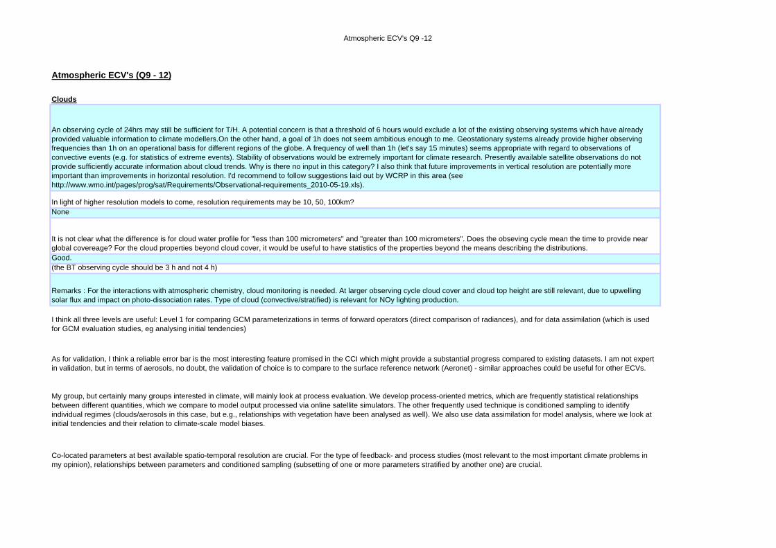
An observing cycle of 24hrs may still be sufficient for T/H. A potential concern is that a threshold of 6 hours would exclude a lot of the existing observing systems which have already provided valuable information to climate modellers.On the other hand, a goal of 1h does not seem ambitious enough to me. Geostationary systems already provide higher observing frequencies than 1h on an operational basis for different regions of the globe. A frequency of well than 1h (let's say 15 minutes) seems appropriate with regard to observations of convective events (e.g. for statistics of extreme events). Stability of observations would be extremely important for climate research. Presently available satellite observations do not provide sufficiently accurate information about cloud trends. Why is there no input in this category? I also think that future improvements in vertical resolution are potentially more important than improvements in horizontal resolution. I'd recommend to follow suggestions laid out by WCRP in this area (see http://www.wmo.int/pages/prog/sat/Requirements/Observational-requirements_2010-05-19.xls).

In light of higher resolution models to come, resolution requirements may be 10, 50, 100km?None

It is not clear what the difference is for cloud water profile for "less than 100 micrometers" and "greater than 100 micrometers". Does the obseving cycle mean the time to provide near global covereage? For the cloud properties beyond cloud cover, it would be useful to have statistics of the properties beyond the means describing the distributions.Good.(the BT observing cycle should be 3 h and not 4 h)

Remarks : For the interactions with atmospheric chemistry, cloud monitoring is needed. At larger observing cycle cloud cover and cloud top height are still relevant, due to upwelling solar flux and impact on photo-dissociation rates. Type of cloud (convective/stratified) is relevant for NOy lighting production.

I think all three levels are useful: Level 1 for comparing GCM parameterizations in terms of forward operators (direct comparison of radiances), and for data assimilation (which is used for GCM evaluation studies, eg analysing initial tendencies)

As for validation, I think a reliable error bar is the most interesting feature promised in the CCI which might provide a substantial progress compared to existing datasets. I am not expert in validation, but in terms of aerosols, no doubt, the validation of choice is to compare to the surface reference network (Aeronet) - similar approaches could be useful for other ECVs.

My group, but certainly many groups interested in climate, will mainly look at process evaluation. We develop process-oriented metrics, which are frequently statistical relationships between different quantities, which we compare to model output processed via online satellite simulators. The other frequently used technique is conditioned sampling to identify individual regimes (clouds/aerosols in this case, but e.g., relationships with vegetation have been analysed as well). We also use data assimilation for model analysis, where we look at initial tendencies and their relation to climate-scale model biases.

Co-located parameters at best available spatio-temporal resolution are crucial. For the type of feedback- and process studies (most relevant to the most important climate problems in my opinion), relationships between parameters and conditioned sampling (subsetting of one or more parameters stratified by another one) are crucial.


In the discussion yesterday, it seemed that "trend analysis" and "process analysis" were regarded separately by ESA, where it was stated that the former need just one parameter, while the latter would need the co-location. I think this is not true. If there is only one parameter available, the trend analysis reduces to one or two PhD theses, which would compute the global-annual mean trend (little work once the data is available), and go deeper by subsetting regions/seasons etc. However, in most cases, trends are probably much more interesting and better to describe if they would be computed on conditioned samples.

Comment on the specification, here referring to the cloud and aerosol ECVs: Trend detection will be challenging, particularly for clouds. I strongly believe it will be of more use to look at processes, for which the long time series would be crucial to provide sound statistics. However, for this type of studies, the resolution is far from adequate. I think the goal should be to have clouds and aerosols at the same resolution, by choosing the better one now given in both cases (i.e., going down to 1 km horizontally for clouds, and temporally down to 1 h for aerosols).In my opinion "threshold" should be set to current standard. The ECV products have to be competitive with (or rather: better than) existing records for them to be used by the community. That is, the threshold resolution should be set to at least 1° horizontal resolution for clouds, and to 1 day temporal resolution for aerosol. If I interpret "breakthrough" as substantially improving on current standards, I think we would want to go below this, where I accept that it might be difficult for the temporal resolution for aerosols. So I suggest for aerosols/clouds the following clouds: T/H 100 km / 6 h; B/T: 10 km / 4 h; Goal: 1 km / 1 h aerosols: T/H: 10 km / 1 d; B/T: 2 km / 1 d; Goal: 1 km / 1h I agree that for the vertically resolved

OzoneNone

For ozone profile - higher stratospher, results of SMILES should be explored.

Ozone : We propose a change in the presentation of the ozone profile in order to better show that the specifications change with the altitude range. We would prefer same threshold specifications for HT and LS for vertical resolution : 2 km. For the LT and tropospheric column, we would prefer 1h/3h/3d for Goal/BT/TH. With a threshold of 2 to 3days, episodes of O3 pollution can be detected and their impacts on a monthly mean is correctly taken into account.NoneGood.

Greenhouse GasesNone

For the detection of CH4 emission from pipe line or small size sources, higher horizontal resolution will be required.

For GHG Same remark on the presentation as for the Ozone table. In the stratosphere, simultaneous observations of CH4 and water vapour would be helpful. The observing cycle specifications could be relaxed in M, HS, LS, HT for CH4 and CO2 : 1 week ?NoneGood.NoneGood.

Aerosols


Similar to comments regarding cloud properties, I think that a coarser resolution (order of 300km) would already be appropriate for category T/H. It seems that a coarser resolution would cover the basic needs for many climate studies (at least studies that are based on GCMs). A resolution of 30km may be appropriate for B/T. Again, vertical resolution is crucial and there is much more potential for scientific breakthroughs there compared to improvements for horizontal resolution. Aerosol vertical profiles are often very inhomogeneous in reality, which severely limits the usefulness of column-integrated observations for aerosols (e.g. for studies of aerosol/cloud interactions). It seems that suggestions by WCRP should be considered in that regard.

The spatial and temporal resolution requirements, especially for the variable lower tropospheric column, may not be in good balance; horizontal resolution is too hard to reach while observing cycle is too coarse to follow synoptic variability.None

Having an observing cycle more in-line with that of the clouds would aid in the understanding of the interactions between the two. This could be done at the expense of reducing the horizontal resolution of the observations.

For aerosols Remark : accuracy of optical depth should be dimensionless. Aerosol measurements are important for atmospheric chemistry, but still not used by our group.

See general comments regarding data for aerosol properties on previous page. It seems useful (and practical?) to retrieve various properties of the aerosol for similar resolution.NoneVaridation of accuracy is important.NoneGood.

Detailed requirements for CCI ECVs It outcomes that together with the questionnaire some definitions would be necessary. Some are given in the GCOS document 107, but it would be worth appending them as their understanding can differ from one to another. In the latest version, the requirements are expressed in terms of G/B/T and here again there would be less ambiguity if the definitions were given. The main remarks concern -the stability : left blank in all the tables - there are no major comment from the CNRM on the tables. Probably because they are too long to be fully analyzed. - Even if it does not outcome from the answers, we guess, however, that the requirements would not be the same according their use, from seasonal (regional) predictions to global projections. For instance : Land cover : For seasonal :spatial sampling 500 m, 25 classes or more would be OK. For global, 1 km and <25 classes We suggest to fix the BKT values as the requirements to be met for general use in the models and take note that higher resolution and time sampling could be needed in the case of regional climate studies.

Q13 -16

Geophysical measurements (q13)

Level 1 16 47.1 %Level 2 21 61.8 %Other 3 8.8 %Total 34 100.0 %

Datasets (q14)What kind of datasets would you like?Single sensor datasets 18 52.9 %Merged product datasets 20 58.8 %Other 2 5.9 %Total 34 100.0 %

Using Super sites, data exchange between ground-based networks, and inter-calibration or validation between different sensors/satellites.

independent validation sites / data

In view of our role as data archivists, our greatest concern is that the validation method should be clearly documented and reproducible. A full decsription of the data used for validation is essential. Documented code would be desirable.Depends on the measurement of course, for column trace gas abundance (CH4 and CO2, what I�m looking at most often), in situ (i.e. aircraft measurements) and ground-based remote sensing (i.e. FTIR) are required.

What is your preferred validation methodology?

(As for land cover, or land related variables:) on the local scale comparison with the ground truth observations. On global scale, comparison with the other satellite products, station data (raw or merged/gridded), archived data (e.g. NSIDC), reanalysis data (NCEP/NCAR, ECMWF, etc.) and other maps (for example produced by USGS, or other expert communities, International Permafrost Association)Not understood the questionOur first order method of validate by comparing climatological statistics between our model and observations. When, and where, possible these statisitics are supplemented by examining relationships between quantities.

What level of geophysical measurements do you require?

Other

Gridded products at monthly resolution, property-property correlations, ability to filter in space and time for multiple variablesLevel 3, gridded monthly statisticsLevel 3 and 4

OtherIntelligently searchable multivariate databases - e.g. the ozone and cloud properties associated with an ensemble of North Atlantic storms (calculated directly via the interface rather than after you have download all of the data yourself)Assimilation products

Preferred validation methodology (q15)

Q13 -16

anycf-net CDF

For the data: NetCDF CF, with additional attributes in the file to ensure it is easily identifiable by man and machine. A good example of the use of additional attributes is provided by the PCMDI CMOR (Climate Model Output Re-writer) package, which is used to standardise climate model output from the Climate Model Intercomparison Project. The file format should be chosen so that the data can be delivered through the same range of services as the climate model output it is intended to validate. For the metadata: An XML document with a well defined schema which clearly defines the instrument, it measurement technique and the analysis used to retrieve the data record. It would be extremely helpful if the schema could, at the top level at least, share some of the structure which has been developed by the EU FP7 project METAFOR to describe climate models and their output. For example, descriptions of institutions could use the same schema elements.

CF complinate Netcdf

We prefer NETCDF files that conform to standard formats.

Sandard format is better for data exchange.HDF5

netcdfCF compliant and netcdf format - but also global means, time series in ascii etc. Flexibility is needed here. Presentation of data in formats other than 'flat' files (one diag, one timeslice) is important (see previous comment on being able to apply spatial and time and property filters to the diagnostics).

netCDF would be more convenient than, say TIFF.netcdf

Ground-based and in-situ data, and comparison of different satellite retrieval techniques (e.g. microwave vs. vis/nir)

Format of data (q16)What is the preferred format for the date? (e.g. CF compliant, NETCDF etc)

NETCDF

Depends on the purpose. Methodologies most useful: - compositing of one variable as a function of another (e.g. clouds as a function of precipitation or dynamical fields) - model-to-satellite evaluations (using a simulator to diagnose from model outputs quantities consistent with level 1 measurements)Against station dataAgainst in situ dataComparison of modelled versus observed ECV Measurement campaigns

The satellite data should be validated with surface data and in-situ measurements where available.

Broad range (based on classical comparison with in situ observation, based on observations-minus-forecast residuals in data assimilation system; ...)

This is a big question. Validation is critical; confidence levels must be reported with the product, to the extent possible. How it is done depends heavily on the variable in question.fire area products require continued evaluation with high resolution (e.g. Landsat) scenes, FRP products require evaluation with new high-resolution instruments (a la BIRD), comparison with burned area products and additional field experiments

Q13 -16

CF compliant NetcdF

NetCDF (but I prefer to a simpler format such as a plain direct access file)HDF or NetCDF

NetCDF! , gridded

NetCDF, binary, Grib, Ascii ... no matterNetcdfNetCDF

NetCDFCOARDS-compliant netcdf4NetCDF or GRIBnetcdf, cf compliant

NetCDF or HDF are acceptable, as long as the data are self-describing, and no separate readme file or metadata is needed to make sense of it.

clearly Netcdf, CF-compliant. Our institute would be happy with the most advanced version (Netcdf4, compatible with HDF)

Q17 - 19

Means of accessing data (q17)What is your preferred means of access to the data?

ftponline

ftp if size is not that large. Maybe DVDs if on GB order.data centres such as PCMDI, NASA/ASDC

ftp

Web-based interfaces to search and locate datasets and non web-based methods to download selected datasets.Depend on the volume.

ftp

FTP/WEBftp and web accessFor large datasets gridFTP is our preferred access method. We are also developing Open Geospatial Consortium (OGC) access tools and would encourage provision of access through a Web Coverage Service.ftp

FTP

FTP, OpenDAP

FTP is usually sufficient, in particular since it allows for automated data download.FTP or Web browserftp, wcsFTP, dodsftpftp

FTP, Web browserFTP, web browserFTP

Web browser, FTP, or OpenDAP; something along the lines of NASA DAAC and EUMETSAT U-MARF, definitely not physical media (e.g. DVD)

clearly FTP, and it would be very helpful to have a web interface allowing for subsetting (in terms of time, region, and parameter)

Use of datasets (q18)

What will your intended use of the datasets be? (e.g. initialisation, assimilation, reanalysis, comparision with models)

comparison with modelscomparison with models

Q17 - 19

comparison with modelscomparison with models; initialization (or boundary conditions)Model validationcomparison with models, assimilationinitialisation, assimilation, reanalysis, comparision with modelsThe main use of the datasets will be for model evaluation.comparison with other sensor data and models.comparisonsassimilations, model validationsI'm more involved with user access to dataProvision of services to the research community.Some surface data is used as input to forward modelling activities (e.g. accurate ice cover, SSTs), while atmospheric data (xCO2 and xCH4, for instance) are used in both inversions for trace fluxes and for comparison with mesoscale forward simulations.My group is mainly interested in process evaluation. For this satellite data are a useful tool for model validation.(global-scale) data assimilationComparison with models, initialisation for climate-prediction model simulations, improvement of parametrisationsDiagnostic analysis of aerosol forcing.operational use in atmospheric composition monitoring (MACC/GMES), chemistry climate modellingMonitoring, comparison with modelsanalysis of the climate system + comparison with modelsComparison with GCMModel evaluationInitialisation, assimilation comparison with modelsinitialisation, comparison with modelsValidation of our GCRM, NICAMComparison with models, reanalysis

General requirements for CCI products (q19)Do you have any other comments

The biggest deficiency in any remote sensing data product is in the delivery of the information. There is nothing like enough time spent creating interfaces and software products to give people what they would ideally like in order to do science. Far too often data is delivered in ways that are convenient for the producers of the data rather than the potential users. There is a huge amount of information that exists in these data streams that is not being accessed because the data download and processing burdens are too large for the end user to handle.

Some of the land surface/near-surface variables (soil moisture, roughness, carbon content/amount, etc.) would be great. Information about water isotopes would be also interesting.Active sensors such as radar and lidar should be also considered for the assimilation or other model uses.easy / simple data access (like NASA data sets, registration to downloading)Regional Climate Modelling Community need more accurate measurements of relative humidity and soil moisture

Q17 - 19

I am filling this in from the perspective of a service provider and leader of a work package in the IS-ENES FP7 project responsible for developing data services to support European archives of ESM data, including the CMIP5 archive. We are very keen to have infrastructure which can, as far as possible, support all data relevant to Earth System Science and would like to cooperate where possible so that our efforts can be complimentary. It is clear that your initiative will be extremely valuable to the climate modelling community. For the CMIP5 archive we are implementing a system based on "data nodes" developed by the Earth System Grid (ESG) Center for Enabling Technologies (a US project) with input from IS-ENES and other collaboraing projects, The data node provides a suite of data access protocols and will be installed in at least 30 modelling and archiving centres to form the CMIP5 distributed archive. This approach allows a standardised set of services to be provided by a wide range of service providers. The same approach is to be adopted for the WCRP CORDEX (downscaling of climate projections) project. Uncertainty in EO data tends to have better characterisation than model output, but it will nevertheless be challenging to represent this in a uniform way. Care should be taken to standardise the terminology across all ECVs.For both CO2 and CH4 the threshold and goal accuracies are far too high to be useful. 10% accuracy on a column measurement that doesn�t even have 10% spatial variability is not very helpful. I could guess the column abundance of methane within 10%! The 1% level for CO2 is getting closer, but an accuracy of better than 1 ppm (around 0.3%) is necessary before any scientific value can be gleaned from the data. I like the temporal resolution of the column data though � every 6 hours would help nail down the diurnal cycle (assuming it�s bigger than the enormous margin of error on the accuracy), and moving that up to every 3 or 4 hours would be great. I�m really surprised that cloud cover isn�t known to a higher horizontal spatial resolution � I�ve been using the 1 km cloud product from MODIS. I may not understand the description of the data product though.Co-located parameters at best available spatio-temporal resolution are crucial.It is absolutely essential for our work that a sea-ice product remains part of this initiative. This is in particular the case given the current public interest in Arctic sea-ice retreat and the fact that changes in sea-ice cover are possibly the most direct indication of climatic changes.

. I'm wondering whether the "Accuracy" columns in Tables 1, 2, etc. represent *instantaneous* measurements, or the statistical average of all measurements made over a fixed period, or something else. 2. In Table 3, Cloud ice profile - Total column, might be "Cloud ice column," and also for water, etc. A "profile" means vertically resolved, in, e.g., g/m3. 3. Is 50 km adequate for Cloud cover? I'm just wondering about places where persistent clouds represent local phenomena. I'd have expected something like 5 or 10 km horizontal resolution, which should be possible to do. Better see what cloud people think about this. 4. Do you really need CO2 every 3-4 hours at 10 or 20 km resolution? 5. How will you obtain *vertically resolved* aerosol optical depth (AOD) globally at a few km resolution daily? Limb sounding can get you stratospheric aerosol, but not globally every day.6. Are the aerosol quantities meant to be spectral or broad-band? 7. Do you want to add aerosol "type"? This would cover whatever size, shape, and single-scattering albedo constraints you can get from the measurements. 8. If you have multi-angle imaging, you could add near-source aerosol plume height, which is very useful for initializing aerosol transport models. 9. The uncertainties in retrieved aerosol parameters tend to vary greatly with observing conditions. A flag indicating data quality would be helpful.Whenever possible, it would be VERY useful to distribute observational datasets in a format, frequency and name similar to CMIP5 model outputs (CMIP5 is the largest set of coordinated model experiments organized by the international modeling community, to be assessed by the IPCC AR5, see http://cmip-pcmdi.llnl.gov/cmip5/)No

Data processing is a huge task. Whenever each user does its own processing starting from level1 it is a big waste. Why not suggest to use level 3 (already averaged) or level 4 Product types, formats and access Table 4 asks for you input on data formats and access options to the datasets. There is a general consensus on the need of level2 products delivered via ftp in cf compliant netcdf. The need of level 1 is also present but inflation of data rate will have to be considered. We can wonder if it would not be important to propose level 3 and 4 .Accuracy for cloud water seems too low: 5-10 Kg/m2; shouldn't it be ~g/m2?

Atmospheric ECVs Q20

Atmospheric ECVs

Priority (q20b) - Precipitation (1)Please rate the priority of the following Atmosphere ECVS.High 17 89.5 %Medium 2 10.5 %Low 0 0.0 %Total 19 100.0 %

Priority (q20b) - Earth Radiation Budget (2)Please rate the priority of the following Atmosphere ECVS.High 17 85.0 % Medium 3 15.0 %Low 0 0.0 %Total 20 100.0 %

Priority (q20b) - Upper-air Temperature (3)Please rate the priority of the following Atmosphere ECVS.High 5 31.3 %Medium 10 62.5 %Low 1 6.3 %Total 16 100.0 %

Priority (q20b) - Upper-air Wind (4)Please rate the priority of the following Atmosphere ECVS.High 6 37.5 %Medium 8 50.0 %Low 2 12.5 %Total 16 100.0 %

Priority (q20b) - Surface Wind Speed and Direction (5)Please rate the priority of the following Atmosphere ECVS.High 9 56.3 %Medium 5 31.3 %Low 2 12.5 %Total 16 100.0 %

Priority (q20b) - Water Vapour (6)Please rate the priority of the following Atmosphere ECVS.High 11 61.1 %Medium 7 38.9 %Low 0 0.0 %Total 18 100.0 %

Q20 comments

Precipitation Earth Radiation Budget Upper-air Temperature Upper-air Wind Surface Wind Speed and Direction Water Vapour

hourly to daily, km scale hourly hourly hourly

Very high priority from a demand perspective both because precipitation has a high societal impact and because models are highly uncertain. There are obvious concerns about the possible length of any EO based precipitation estimates, but I believe that the utility of what is available is high. There are, for instance, still considerable problems with the way climate models represent the diurnal cycle of precipitation and EO datasets which can provide a relevant observational baseline.

A key component of the Earth's energy budget, could play a major role in validating climate models.

In particular snow (with density estimate)

Vertical profiles of precipitation would be very useful to evaluate convection schemes in climate models

Tropospheric chemistry

There is a consensus on the need of additional Atmosphere ECV. There are discrepancies in the answers on Terrestrial. They are certainly due to the different applications targeted.I simply marked with 'H' to which I usually refer for model validation, and with 'M' for others

Q20 comments

As for other ECVs which should be added to the list, I very strongly advocate for the Earth Radiation Budget. This is the one quantity which is of most fundamental interest for climate change. Forcings and climate feedbacks cannot be determined unless the energy balance of the system is known. For this budget, high-quality, long-term satellite observations are crucial. The ERB satellite measurements cannot be replaced by any other observation. I suggest the ECV should contain products split into short- and longwave components, and be reported jointly with the cloud ECV so a computation of the cloud radiative effects would be possible.

Of further crucial importance are for analyses of the hydrological cycle, and of relevant climate processes, in descending order: water vapour; precipitation; soil moisture.Particularly water vapour would be of great help to climate modelling, especially if provided as relative humidity, if vertically resolved, and if at good spatial resolution.

Marine ECVS

Priority (q21b) - Sea State (1)Please rate the priority of the following Marine ECVS.High 3 23.1 %Medium 5 38.5 %Low 5 38.5 %Total 13 100.0 %

Priority (q21b) - Ocean Salinity (2)Please rate the priority of the following Marine ECVS.High 7 50.0 %Medium 4 28.6 %Low 3 21.4 %Total 14 100.0 %

Sea State Ocean Salinity

Not an oceanographer Idem

Priority (q22b) - Snow Cover (Extent, Snow Water Equivalent) (1)Please rate the priority of the following Terrrestrial ECVS.High 13 72.2 %Medium 5 27.8 %Low 0 0.0 %Total 18 100.0 %

Priority (q22b) - Permafrost and seasonally-frozen ground (2)Please rate the priority of the following Terrrestrial ECVS.High 8 47.1 %Medium 9 52.9 %Low 0 0.0 %Total 17 100.0 %

Priority (q22b) - RIver Discharge (3)Please rate the priority of the following Terrrestrial ECVS.High 7 41.2 %Medium 6 35.3 %Low 4 23.5 %Total 17 100.0 %

Priority (q22b) - Lake levels (4)Please rate the priority of the following Terrrestrial ECVS.High 1 5.9 %Medium 10 58.8 %Low 6 35.3 %Total 17 100.0 %

Priority (q22b) - Albedo (5)Please rate the priority of the following Terrrestrial ECVS.High 14 77.8 %Medium 4 22.2 %Low 0 0.0 %Total 18 100.0 %

Priority (q22b) - fAPAR (6)Please rate the priority of the following Terrrestrial ECVS.High 1 6.3 %Medium 13 81.3 %Low 2 12.5 %Total 16 100.0 %

Priority (q22b) - Leaf Area Index (7)Please rate the priority of the following Terrrestrial ECVS.High 6 31.6 %Medium 11 57.9 %Low 2 10.5 %Total 19 100.0 %

Priority (q22b) - Biomass (8)Please rate the priority of the following Terrrestrial ECVS.

Terrestrial ECVs

High 4 21.1 %Medium 12 63.2 %Low 3 15.8 %Total 19 100.0 %

Priority (q22b) - Soil Moisture (surface and root zone) (9)Please rate the priority of the following Terrrestrial ECVS.High 14 77.7 %Medium 4 22.3 %Low 0 0.0 %Total 18 100.0 %

Q22 Comments

Snow Cover (Extent, Snow Water Equivalent)

Permafrost and seasonally-frozen ground RIver Discharge Lake levels Albedo fAPAR Leaf Area Index Biomass

Soil Moisture (surface and root zone)

We want to assimilate fractional snow cover and SWE product in to the ECHAM5 model.

hourly

daily; evaporation / transpiration needs special attention

The biosphere is a crucial part of the Earth system, and there should be at least one biosphere component among the CCI outputs � if possible (I suggest this should be Leaf Area Index, but am not qualified to judge whether this is the most appropriate of the biosphere variables to prioritise).

Important for methane modelling of course, and of great interest for simulating present climate, and estimating carbon release in future climate scenarios.

Again, important for methane modelling, but what would really be good to have is a remotely sensed estimate of wetland extent from season to season � the disagreement between currently used maps is alarming.

?

Including SWE.New component of climate model to be validated globally + river width at river mouth ?

Not crucial for global hydrology

Distinction between bare ground and vegetation ?

Not crucial for global hydrology (but relevant for carbon cycle)

Not crucial for global hydrology (but relevant for carbon cycle)

Not crucial for global hydrology (but relevant for carbon cycle) Including root zone

Absolutely needed, from weather forecasting to improvements / testing of land surface models

improvements / testing of land surface models and basic knowledge of the processes in the Arctic

Useful when/where no in-situ data available

improvements / testing of land surface models




Absolutely needed, from weather forecasting to improvements / testing of land surface models

is

d1.1 profile and needs of cmc - esa climate office

Documents