d1 introduction to distribution systems module...

D1 Introduction to Distribution Systems 230

All materials are under copyright of PowerLearn. Copyright © 2000, all rights reserved.

Module D1

Introduction to Distribution Systems

Primary Author: Gerald B. Sheble, Iowa State University

Email Address: [email protected]

Prerequisite Competencies: Steady State analysis of circuits using phasors, three-phase circuit

analysis and three-phase power relationships, found in Module B3.

Module Objectives: 1. Identify basic distribution substation equipment including

transformers and protection equipment.

2. Perform distribution circuit voltage regulation and power

efficiency calculations.

3. Perform power factor correction calculations for large industrial

loads.

4. Identify basic wiring requirements for residential and commercial

installations including wiring color codes and grounding

requirements.

Distribution Overview

Energy is consumed at a nominal voltage of 120 or 240 volts for most residential equipment and 208, 240, 277 pr

480 volts for commercial and industrial customers. The power flows through a metering device to determine the

amount of real power consumed by the equipment. The reactive power is provided without charge. The exception

to this is if commercial or industrial customers operate at a low power factor, they could incur a power factor

correction change.

The distribution system transports the complex power from the transmission grid to the customer. Distribution

systems are typically radial because networked systems, although more reliable, are more expensive. Since three-

phase power is more efficient than single phase, sets of three lines start from each distribution substation. However,

close to the end of the radial feeder, it is often efficient to drop one or two of the three phases. Often only a single

phase is used in very rural areas to reach the most remote customers. This less expensive design results in uneven

loading of all three phases. The loading is equalized as much as possible by proper assignment of customers to each

phase. It is the selection of the line capacities, number of phases over distance, the setting of transformers, voltage

levels and customer geographic distribution and usage which complicates the engineering task of distribution design.

D1.1 Equipment Description / Functions

The equipment associated with the distribution system includes the substation transformers connected to the

transmission grid (network), the distribution lines from the transformers to the customers and the protection and

control equipment between the substation distribution transformer and the customer. The protection equipment

includes lightning protectors, circuit breakers (with or without reclosers), disconnects, and fuses. The control

equipment includes voltage regulators, capacitors, and demand side management (load control) equipment.

The substation transformers typically reduce the transmission grid voltage from 138 kV to 69, 34.5 or 12 kV. Older

distribution systems may still use four kV as the primary voltage. The distribution lines are radially configured, due

to cost considerations. However, large city distribution may be networked. Especially if the system is underground

through a number of large buildings previously connected by steam pipes or coal distribution network.

mailto:[email protected]



Distribution lines are three-phase on leaving the substation but are often reduced to two-phases or one-phase for

loads distant from the substation. The loading of each phase at the substation is as equal as possible barring unusual

load usage patterns by assigning customers to each phase based on historical usage. The substation transformer

reduces any final load imbalance by appropriate design of the secondary windings.

The loading of each phase is distributed equally under normal conditions and normal load patterns for the customers

connected to the distribution line.

The control devices include voltage regulators and capacitors. Both devices attempt to raise the voltage to reduce

the losses and to provide the proper voltage at the customer location. A voltage regulator is an autotransformer with

tap positions to raise the voltage to a target value. A capacitor has a timer or a voltage-sensing device to connect the

device when the voltage is below a target level. A new device used for large commercial or industrial customer is a

static var controller (SVC). A SVC consists of inductors and capacitors that are switched into use by power

electronic circuits to implement a desired control. A desired control may be a desired voltage or a desired harmonic

content of the voltage (see module PQ1). Similar devices are considered as FACTS devices. FACT is a pneumonic

for flexible AC transmission system. These devices use microprocessor technology to sense the real-time conditions

of the system and respond, normally within a quarter of a cycle or less, to electronically switch components.

Components are either inductors or capacitors.

The protection equipment includes lightning protectors, fuses, disconnects and breakers. Lightning protectors

(arrestors) remove high voltage surges by switching the line to ground using spark gaps. Once the spark gap voltage

limit has been exceeded, magnetic fields established by the flowing current by coils extend the arc to increase the

voltage need to sustain the arc, thus extinguishing the arc when the voltage returns to normal. A typical resistance

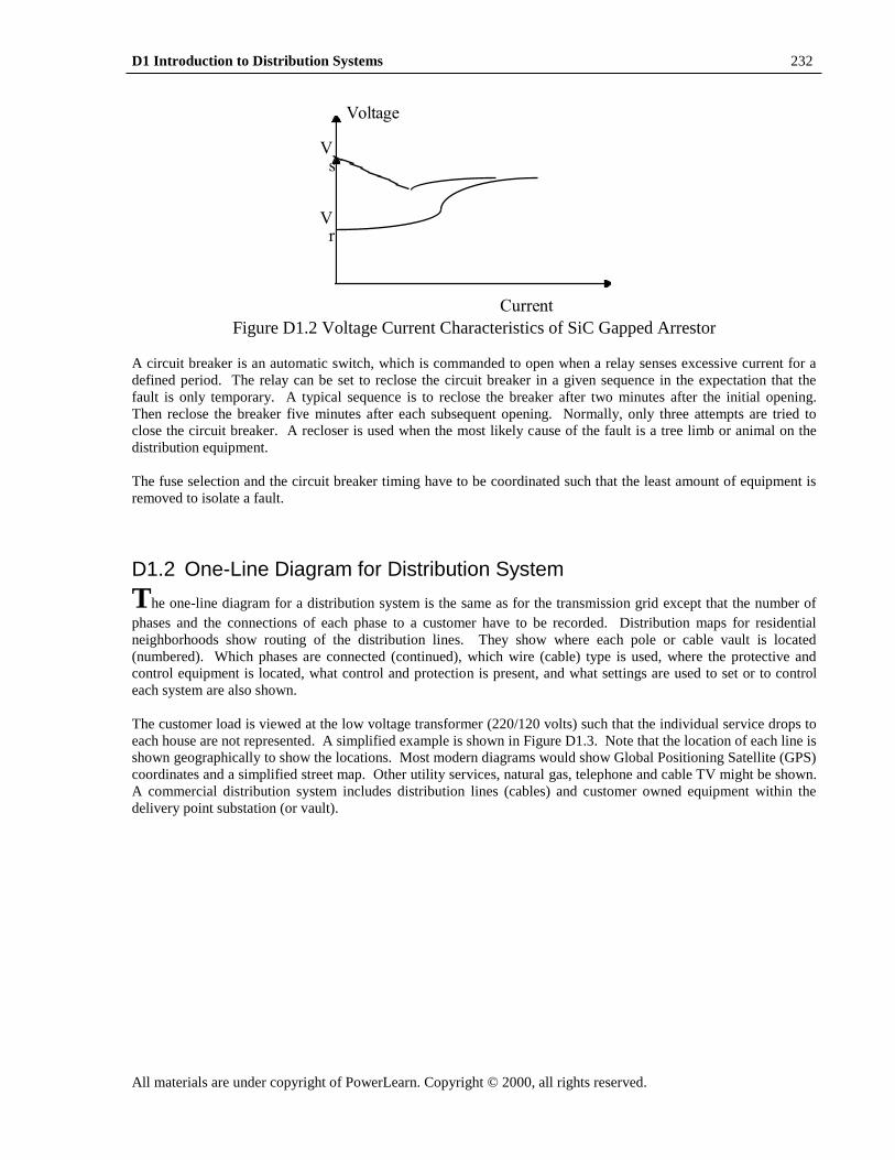
versus voltage graph is shown in Figure D1.1. Note that this is a nonlinear device.

Resistance

Voltage Figure D1.1 Lightning Arrestor Impedance Model

A sequence of events, shown as a graph of current versus voltage for a typical lightning arrestor is shown in Figure

D1.2. As the voltage increases to the strikeover value (Vs), the device starts to conduct very quickly, resulting in a

fast increase in current connected to ground. After sufficient current has passed to de-energize the excessive

voltage, the current will decrease until the reclosing voltage (Vr) is reached when the device stops conducting.

Fuses and circuit breakers are used to isolate the distribution system when a fault occurs on the distribution line. A

fault is simply the failure of one or more components of the system. Typical distribution faults include wire on

ground after object (car, plane, etc.) hits pole, thereby breaking pole. Other faults can be temporary. One typical

temporary fault is a tree limb touching the distribution wire. The tree conducts electricity to ground. Another

typical temporary fault occurs when a biological object (bird, squirrel, human, etc.) connects the distribution wire to

ground. A fuse is simply a piece of metal with a lower melting point than the distribution line wire. When a fault

occurs on the line, a significantly higher current flows. This causes the metal to melt, an arc results clearing the path

of all metal and the arc is extinguished since the normal operating voltage can not sustain the arc. The amount of

overcurrent determines how quickly the fuse melts.



Voltage

V s

V r

Current Figure D1.2 Voltage Current Characteristics of SiC Gapped Arrestor

A circuit breaker is an automatic switch, which is commanded to open when a relay senses excessive current for a

defined period. The relay can be set to reclose the circuit breaker in a given sequence in the expectation that the

fault is only temporary. A typical sequence is to reclose the breaker after two minutes after the initial opening.

Then reclose the breaker five minutes after each subsequent opening. Normally, only three attempts are tried to

close the circuit breaker. A recloser is used when the most likely cause of the fault is a tree limb or animal on the

distribution equipment.

The fuse selection and the circuit breaker timing have to be coordinated such that the least amount of equipment is

removed to isolate a fault.

D1.2 One-Line Diagram for Distribution System

The one-line diagram for a distribution system is the same as for the transmission grid except that the number of

phases and the connections of each phase to a customer have to be recorded. Distribution maps for residential

neighborhoods show routing of the distribution lines. They show where each pole or cable vault is located

(numbered). Which phases are connected (continued), which wire (cable) type is used, where the protective and

control equipment is located, what control and protection is present, and what settings are used to set or to control

each system are also shown.

The customer load is viewed at the low voltage transformer (220/120 volts) such that the individual service drops to

each house are not represented. A simplified example is shown in Figure D1.3. Note that the location of each line is

shown geographically to show the locations. Most modern diagrams would show Global Positioning Satellite (GPS)

coordinates and a simplified street map. Other utility services, natural gas, telephone and cable TV might be shown.

A commercial distribution system includes distribution lines (cables) and customer owned equipment within the

delivery point substation (or vault).



TSS:Electric

Junction

Fast Foods

Shipping Cos

Mobile

Home

Courts

Foodstores

Screen

Shows 5

Lincoln Way

Grand to Duff

Note: map is not to scale

Lincoln Way

Duff to

Skunk River

South

Marlotan

Ave

West Farm

AccessWest So

15th Street

North

Figure D1.3 Distribution System One-Line Diagram

Light industrial systems are normally at higher voltages (e.g. 34.5 and 69 kV) and are always three phases.

Industrial distribution systems may be served at even higher voltages (e.g. 69, 138, 230 and 345 kV). Such loads are

directly connected to the transmission grid (all three phases).

D1.3 Load Types

The load equipment at a customer location includes many different devices, which may be categorized into the

following types: resistive, inductive, and (very infrequently) capacitive. The actual loads are primarily resistive for

heating, inductive for motors, and capacitive for filtering. However, power electronics can change the actual load

into an alternative characteristic by high speed switching and signal conditioning. Capacitors may also be present

for power factor correction. These are control devices and not loads from the customer perspective.

The customer models are generated from surveys of home appliances based on the econometrics of each

neighborhood. Additionally, load profiles are available from chart records at each substation per distribution feeder.

Such charts are normally available for each month of the year. Digital recording of feeder loads is more prevalent

and allows more extensive modeling of the customer use patterns.

In addition, the power factor of each feeder is recorded to determine if corrective action is required. The use of

power electronic motor drives and power supplies are quickly changing the characteristics of load devices.

D1.4 Design Guidelines

The primary regulator design guide is the voltage target at the customer location. The voltage magnitude is

required to be between 110 and 125 volts at the customer side of the low voltage transformer. State commissions set

this limit. Additionally, voltage dips at the customer site are required to be within specified limits in most states.

The voltage will dip as the inrush currents for starting machines temporarily load the system.

The state commissions also typically set reliability targets for the customer. Such considerations are beyond the

scope of this text.

The power quality at the customer site is also a concern as covered in Module PQ1. Power quality now involves

many aspects of delivery including frequency, harmonic content, reliability, etc. This text assumes that power

quality only includes harmonic content. Other delivery specifications are discussed individually.

Any special load considerations may have to be considered by the electric utility, when such loads adversely affect

the distribution system. Such considerations are beyond this text.



D1.5 Customer Tariffs

The customer pays for electricity according to the tariff approved by the state public utility commission. An

example of such tariffs would contain the following details:

Residential Tariff: Price for electric usage is $0.05/kWHr. The electricity delivered is nominally 60 Hertz, 105-130

volts AC, with no more than one hour of interruption per year.

Light Industrial Tariff: Price for electric usage is $0.10/kWHr energy charge and $0.15/kW demand charge for the

peak demand in any half-hour interval. The electricity delivered is nominally 60 Hertz, 105-130 volts AC, with no

more than one day of interruption per year.

Medium Industrial Tariff: Price for electric usage is $0.15/kWHr energy charge and $0.20/kW demand charge for

the peak demand in any fifteen-minute interval. Power factor correction charge is assessed if the power factor is less

than 0.95. The power factor correction charge is $0.50/kVAr for correcting demand below 0.95 and $0.70/kVAr for

correcting demand below 0.90. The electricity delivered is nominally 60 Hertz, 105-130 volts AC, with no more

than eight hours of interruption per year.

Heavy Industrial Tariff: Price for electric usage is $0.18/kWHr energy charge and $0.25/kW demand charge for the

peak demand in any fifteen-minute interval. Power factor correction charge is assessed if the power factor is less

than 0.98. The power factor correction charge is $0.50/kVAr for correcting demand below 0.98 and $0.70/kVAr for

correcting demand below 0.95. The electricity delivered is nominally 60 Hertz, 105-130 volts AC, with no more

than one hour of interruption per year.

The above tariffs are only examples. Practical tariffs vary greatly. However, the above detail is exemplary of the

detail of most tariffs. Note that each state has a different tariff structure and price philosophy for each customer. It

is common for states to give preferential treatment to companies who relocate into a state from another state or

country. Such preferential treatment is termed cross subsidies since the total cost of production, transportation,

distribution and financing of the utility has to come from electricity sales. Income is derived primarily from sales.

Thus, other customers must pay for the preferential treatment of others. Such cross subsidies are extremely political

in nature. The amount and number of cross subsidies is very large and is one of the focal points for de-regulation of

electric utilities.

This module assumes that the customer will be charged an energy charge, a capacity charge, and a power factor

correction charge. Table D1.1 lists the assumed charges for the examples in this chapter.

Table D1.1 Pricing Data Tariff Factor Qualifying factor Rate

Energy Charge $0.10/kWHr

Demand Charge $0.05/kVAr

Power Factor Correction Pf less than 0.95 $0.10/kVAr

Pf less than 0.9 $0.30/kVAr

Pf less than 0.85 $0.40/kVAr

This module also assumes that the cost and price estimates can be based on a single analysis for the peak period.

The assumption is that the peak period is one hour of the 8,760 hours per year. The costs of this peak period can be

used as an estimate of the yearly cost if a functional relationship can be found. Assume, for the examples, that the

peak period can be multiplied by a utilization factor and then by the number of hours in a year to estimate the

income and the costs for the year. Use a utilization factor of .6 for the examples in this chapter. The marginal cost

for the peak period is an index to use for cost estimates. The marginal cost is the cost of adding one more increment

of demand when all other parameters stay fixed.



D1.6 Distribution System (Voltage Drop) Calculations

We will describe voltage regulation calculations for a radial system. Single-phase calculation will be used as

distribution feeders are often single phase. For three-phase distribution circuits we must use a per-phase equivalent

circuit.

Power flow equations (conservation of energy) are solved by assuming a voltage at the most remote point (the

receiving end) of the distribution system such that the voltage will be within the required range. The receiving end

voltage is set to the target; the receiving end current is calculated from the complex power demand at the receiving

end, then the sending end voltage and current are calculated for the receiving end values. This process is iteratively

used for each load until the voltage at the transmission substation is calculated. The load demand could be a

constant power drain (sink). The load demand could be a constant current sink. The load demand could be constant

impedance. The type of load demand may even be a composition of all three load types.

The recursive steps in the process are broken down into the following. First, assume a voltage at the farthest end

(last customer). Use this voltage to find the current at the customer bus. Find the sending end voltage and current

for this distribution segment. Use the voltage at this bus to find the current required for the customer at this bus.

Add to this current the current needed for any distribution lines leaving this bus. Now repeat the process until the

voltage at the sending end bus (transmission substation) is found.

The procedure for distribution calculations can be depicted by the following pseudo-code in Table D1.2. This

procedure is implemented in MATLAB code for the corresponding simulator.

Table D1.2 Voltage Regulation Calculations 1. For the last customer calculate the current for the required voltage:

a. If impedance load, then use ohm’s law,

b. If power load, then use S=VI*.

2. Calculate the sending end voltage and current using current from 1.

3. For the next customer calculate the current for the required load

(sending end voltage from 2.):

a. If impedance load, then use ohm’s law,

b. If power load, then use S=VI*.

4. Calculate the total current, using KCL to find the current required from the next line toward

the source.

5. Calculate the sending end voltage and current matrix using current from 4.

6. Repeat steps 3 through 5 for all customers and lines until the source is reached.

7. Calculate the sending end power from S=VI*.

10. Calculate the voltage regulation (Vs-Vr)/Vr.

The voltage regulation is calculated as shown in (D1.11). The voltage regulation is a measure of the stiffness of the

distribution system. Ideally, the voltage regulation at all load buses should be small. However, a recurring problem

is voltage flicker due to motor start-up inrush currents. The presence of such flicker is an indication that the

distribution system is not stiff and that significant voltage correction is needed.

%100*s

Rs

V

VVVR

(D1.11)

Once all line currents are known, then the losses can be completed as the sum of I2R over all lines. Then efficiency

is

IN

LOSSIN

P

PP

where PIN is the power from the source.



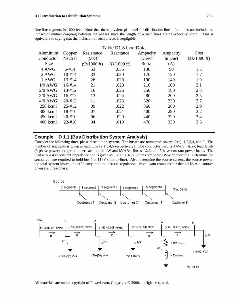
One line segment is 1000 feet. Note that the equivalent pi model for distribution lines often does not include the

impact of mutual coupling between the phases since the length of a such lines are "electrically short." This is

equivalent to saying that the inclusion of such effects is negligible.

Table D1.3 Line Data Aluminum

Conductor

Size

Copper

Neutral

Resistance

(90c)

(/1000 ft)

Reactance

(/1000 ft)

Ampacity

Direct

Burial

Ampacity

In Duct

(A)

Cost

($k/1000 ft)

4 AWG 6-#14 .53 .035 130 90 1.5

2 AWG 10-#14 .33 .030 170 120 1.7

1 AWG 13-#14 .26 .029 190 140 1.9

1/0 AWG 16-#14 .21 .028 210 160 2.1

2/0 AWG 13-#12 .16 .026 250 180 2.3

3/0 AWG 16-#12 .13 .024 280 200 2.5

4/0 AWG 20-#12 .11 .023 320 230 2.7

250 kcml 25-#12 .09 .022 360 260 2.9

300 kcml 18-#10 .07 .021 400 290 3.2

350 kcml 20-#10 .06 .020 440 320 3.4

400 kcml 22-#10 .04 .019 470 330 3.6

Example D 1.1 (Bus Distribution System Analysis) Consider the following three-phase distribution system. The busses are numbered: source (src), 1,2,3,4, and 5. The

number of segments is given in each line (2,1,3,4,5 respectively). The conductor used is 4AWG. Also, load levels

(3-phase power) are given under each bus in kW and kVARs. Buses 1,2,3, and 5 have constant power loads. The

load at bus 4 is constant impedance and is given as (12000+j4000) ohms per phase (Wye connected). Determine the

source voltage required to hold bus 5 at 11kV (line-to-line). Also, determine the source current, the source power,

the total system losses, the efficiency, and the percent-regulation. Note again compensator that all kVA quantities

given are three-phase.



Aj

j

V

SI

V

3533.04021.0306350

103

210

3063503

3011000

3

5

5

7291.07353.037575.033318.03533.04021.0

37575.033318.0400012000

002.303.6352

002.44.11002

002.303.6352175.065.23533.4021.0306350

454

4

44

4

45554

jjjIII

jjZ

VI

V

jjZIVV

S

S

LL

0055.24212.22765.16859.17291.07353.0

2765.16859.1006.3046.6354

103

540

006.25.11006

006.3046.635414.012.27291.07353.0002.303.6352

343

3

3

3

34443

jjjIII

j

j

I

V

jjZIVV

S

S

LL

0106.55299.500506.310674.30055.24212.2

00506.310674.30106.3044.6359

103

2080

0106.88.11014

0106.3044.6359105.059.10055.24212.2006.3046.6354

232

3

2

2

23332

jjjIII

j

j

I

V

jjZIVV

S

S

LL

5158.91847.1050523.46568.40106.55279.5

50523.46568.40158.3036.6363

103

30120

0158.66.11021

0158.3036.6363035.053.00106.55299.50106.3044.6359

121

3

1

1

12221

jjjIII

j

j

I

V

jjZIVV

S

S

LL

0372.98.11046

0372.3097.637707.006.15158.91847.100158.3036.6363

,

111

LLSRC

SSRC

V

jjZIVV

Wjj

jIVPP

II

SRCSRCINSRC

SRC

198.77562029.85056066.25854Re3029.85056066.25854Re3

5158.91847.100372.3097.6377Re3Re3

1



LOSS

S

PTOTAL

RI

RI

RI

RI

RI

Losses

)19.254(3

935.205

502.29

716.15

273.2

7592.

:

12

1

122

2

232

3

342

4

452

5

%425.0%10098.11046

1100098.11046%

%100%

:%

,

5,,

reg

V

VVreg

regregulation

SRCLL

LLSRCLL

%02.99%100198.77562

57.762198.77562

%100

:

IN

LOSSIN

P

PP

Efficiency

D1.7 Split Distribution Line Analysis

The student should determine how to solve the equations if the distribution line splits into two sections as shown

in Figure D1.6. Note that the calculations are a problem when the two distribution lines connect at bus 2. The

solution is to invent an iterative procedure to adjust the customer voltage at bus 6 until the voltages at the connection

point are (nearly) the same.

An example procedure is to update the ending voltage (customer 5) assuming that the last three solutions can

approximate a quadratic curve to find the same solution as found for the first branch (Customers 2 and 3).

Other power flow techniques, such as Gauss-Seidel, are typically used. Such techniques are the subject of senior

elective or graduate courses.

Source

Customer 1

Customer 4

Customer 3

4

DL-1 DL-2 DL-3

Customer 2

DL-4

3 2 1

Customer 5

DL-6 DL-5

5

6

Figure D1.6 Multiple Branch Distribution System



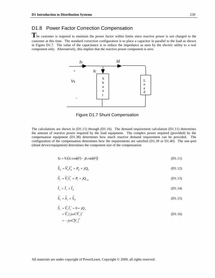
D1.8 Power Factor Correction Compensation

The customer is required to maintain the power factor within limits since reactive power is not charged to the

customer at this time. The standard correction configuration is to place a capacitor in parallel to the load as shown

in Figure D1.7. The value of the capacitance is to reduce the impedance as seen by the electric utility to a real

component only. Alternatively, this implies that the reactive power component is zero.

The calculations are shown in (D1.11) through (D1.16). The demand requirement calculation (D1.11) determines

the amount of reactive power required by the load equipment. The complex power required (provided) by the

compensation equipment (D1.38) determines how much reactive demand requirement can be provided. The

configuration of the compensation determines how the requirements are satisfied (D1.39 or D1.40). The one-port

(shunt device/equipment) determines the component size of the compensation.

sincos dddd jIIVS (D1.11)

ddddd jQPIVS * (D1.12)

dccccc jQPIVS * (D1.13)

dcs III (D1.14)

dcs SSS (D1.15)

2

*

*

)(

0

c

cc

cccc

VCj

VCjV

jQIVS

(D1.16)

L o a d

S

h

u

n

t

>

+

-

Vs

Is Id

Ic

Figure D1.7 Shunt Compensation



Example D 1.2 (Power Factor Correction)

Consider a one demand operating at 500V at 60 Hz with P1 = 48kW @ pf = 0.60 lagging and P2 = 24 kW at pf =

0.96 leading. Add a capacitor in parallel to these and find the capacitance value to zero the reactive demand.

kVAjjQPS 6448111

kVAjjQPS 724222

laggingpfkVAkVAjQQjPPSnet [email protected]

netc QkVArQ 57

VVc 500

sec

377rad

FVQC cc 605/2

Other compensation configurations and calculations may be required for unique load conditions. Inductors may also

be added to compensate for excessive capacitance at the customer site.

Alternatively, automatic compensation may be required if the load characteristics change quickly. A power

electronic device called a static VAR or voltage compensator (svc) as mentioned above (D1.1) accomplishes such

automatic compensation. The power system specialist should be able to derive all of the equations needed for

compensation by shunt inductors, series capacitors, or series inductors.

D1.9 Balancing Power Feeder Demands

Distribution line load demands are "balanced" by dividing the number of customers between the three phases such

that the expected demand (kVA) is evenly divided. The amount of demand per customer has to be known or

estimated as well as the time schedule for the demand. Then the demand amount and schedule is used to determine

to which phase the customer should be connected. If the demand is unknown, then it is typical to use the rated

capacity of the pole transformer as the customer demand.

Consider a feeder, which has a loading profile of (A-120, B-60, and C-100), all in kVA at a given point on the line.

The next customer closest to the distribution substation to be added is expected to demand 40 kVA. This customer

should be placed on the B phase to yield a resulting loading profile of (A-120, B-100, C-100). Thus this process

starts at the farthest point of the feeder and completes at the distribution substation. The same process is used if only

two of the phases are present. Obviously, if only one phase is present, there is no decision to be made.

An example calculation would be to divide the loads in Table D1.4 among the three phases as shown. Note that the

feeder requires only the c phase to extend to the last customer and only the b phase to extend to the second to last

customer. Thus, one would only find one phase at the end of the circuit, two phases as the circuit is traced to the

source. Note that loading is not equal. Note that the demand is only an estimate and does not contain information as

to the time of day when the demand will occur. This data is normally adopted from typical demand patterns for

typical homes on typical days. Almost as accurate as a weather forecast!

If the distance between customers is large compared to the cost of line, then the number of phases extended to the

last customers can be significantly changed as shown in Table D1.5.



Note that phase A does not extend beyond the fifth customer. Phase B does not extend beyond the ninth customer.

Thus, the number of conductors can be reduced to save costs. Additionally, the complexity of the pole top design to

carry one conductor is simpler than for three. Also, less expensive. The economics of installation will determine

the approach taken.

The student may wish to consider the reliability of the circuit. Would the extension of all three phases to the last

customer provide service that is more reliable? Under what conditions would the service be more reliable? Under

what conditions would the service be of the same reliability?

Table D1.4 Distribution Customer Data (Plan A)

Customer Demand

(kVA)

Phase A Phase B Phase C

1 10 10

2 35 35

3 40 40

4 20 20

5 10 10

6 35 35

7 15 15

8 25 25

9 30 30

10 05 05

11 25 25

12 15 15

13 15 15

14 30 30

Total 115 105 90

Table D1.5 Distribution Customer Data (Plan B)

Customer

Demand

(kVA)

Phase A Phase B Phase C

1 10 10

2 35 35

3 40 40

4 20 20

5 10 10

6 35 35

7 15 15

8 25 25

9 30 30

10 05 05

11 25 25

12 15 15

13 15 15

14 30 30

Total 115 105 90



D1.10 Tolerance of Current

Table D1.6 shows the current impact on the human body. Note that the amount of current is measured in milli-

amps. Whereas, the current in a distribution system is normally measured in kilo-amps.

Table D1.6 Tolerance of Current - Humans

Current Effect

1-5 mA Sensation

10-20 mA Involuntary muscle contractions

20-100 mA Pain, breathing difficult

100-300 mA Ventricular fibrillation, possible death

>300mA Respiratory paralysis, burns, unconsciousness, permanent loss of short-term memory,

compaction of soft tissue (spinal cord, etc.)

D1.11 Customer Wiring

The distribution transformer connected between the distribution line and the customers may be configured in a

number of ways. The configuration is based on selected practice (preferences) and economic cost. Once in the

customer’s site, the wiring is the responsibility of the customer. The National Electric code requires all designs to

be within 125% of equipment capability. Figure D1.8 shows how a single-phase connection can be transformed into

a two-phase connection. Note that the key is to ground the middle of the secondary coil to be the reference for the

customer.

12kV

120 V

120 V

Figure D1.8 Distribution to Customer Wiring Transformation

Figure D1.9 shows a typical distribution box found in most residential and commercial facilities. The incoming

phases (2) are connected to a main circuit breaker to isolate the customer from the source if current exceeds a

maximum (typically 100 or 200 amps). The main circuit breaker is connected to two (2) bus bars to which

individual circuit breakers are attached. The basic circuit breaker will feed one or two rooms and is limited to 15 or

20 amps. Note that the black wire is always assumed hot unless the circuit breaker is open. The white is the normal

return (ground). The green wire is the safety ground. The safety ground protects the user by providing a lessor

resistance path from the appliance to ground as shown in Figure D1.10.



Figure D1.9 Residential Distribution Panel

Appliance with safety ground

Appliance without safety ground

Water Pipe

Ground

Figure D1.10 Safety Ground Principles

black

white

green

blackblack

white

240 V

120 V

MAIN

+120 V

-120 V

ground



A special circuit breaker, called a Ground Fault Interrupter (GFI), can be used to provide more protection to the

user. As shown in Figure D1.11, the GFI senses the amount of current flowing to the appliance(s). If the amount of

current flowing on the hot (black) wire is not equal to the current flowing in the white wire, or if there is any current

flow through the green wire, then the circuit breaker is opened. Note that many residences have a GFI installed in

the wall box instead of in the distribution panel. The circuit breaker in the distribution box is then a normal circuit

breaker. The National Electrical Code (NEC) requires GFIs in any room where the user may come in contact with a

water pipe or the water tables (kitchen, bath, outdoors, etc.). Consider that almost all water pipes are metal and are

connected to ground through a small resistance compared to most building materials. The concern is that the

appliance may become defective and the current would return to the ground through the user. Figure D1.11 shows

the protection provided by a GFI when a user uses a metal instrument (knife) to remove bread from a toaster. Most

users would prefer a GFI to start the day in a better way.

Appliance with safety ground and GFI

Appliance without safety ground

Water Pipe

Ground

Figure D1.11 Application of Ground Fault Interrupter

The student should consider alternative grounding problems such as the “stray voltage” problem. The stray voltage

problem has occurred in many farm facilities. This problem occurs when the ground is of high resistance compared

to alternative current paths. An alternative current path may be a building, natural gas pipes, railroad tracks, etc.

Metal structures within the building are the primary problem. Consider what would happen if an animal or a human

touched a handrail or a metal feeder which is at a higher voltage than the ground underneath the feet. The electrons

always find the least resistance path independent of the discomfort to the biological entity. This is often a serious

problem, since animals cannot say that they feel the power. The result is often a cow that will not eat or allow

anyone to hook up the milking machine. If farm equipment is improperly installed the currents can be sufficiently

high to kill.

D1.11 Two Port Circuits

The treatment below is largely adapted from [1]. In performing circuit analysis of single phase distribution systems,

it is often convenient to make use of two-port theory. A two-port network is one with two pairs of terminals

emerging from it such that, for each pair of terminals, the current entering one terminal is the same as the current

leaving the other terminal. Figure D1.12 illustrates a generalized two-port network. We require that there be no

independent sources in the network (dependent sources are allowed), and there can be no energy stored in the

network.



+

V1

-

+

V2

-

I1

I2

Two Port

Network

Fig. D1.12: Generalized Two-Port Network

Passive two-port networks are commonly specified in terms of their network parameters, according to the following

expressions:

Z (impedance) parameters

2

1

2

1

2221

1211

2

1

I

IZ

I

I

zz

zz

V

V (D1.17)

Y (admittance) parameters

2

1

2

1

2221

1211

2

1

V

VY

V

V

yy

yy

I

I (D1.18)

H (hybrid) parameters

2

1

2

1

2221

1211

2

1

V

IH

V

I

hh

hh

I

V (D1.19)

G (inverse hybrid) parameters

2

1

2

1

2221

1211

2

1

I

VG

I

V

gg

gg

V

I (D1.20)

a (transmission) parameters

2

2

2

2

2221

1211

1

1

I

VA

I

V

aa

aa

I

V (D1.21)

b (inverse transmission) parameters

1

1

1

1

2221

1211

2

2

I

VB

I

V

bb

bb

I

V (D1.22)

In using two ports, it is assumed that only voltages and currents at the terminals are of interest, i.e., there is no

interest in computing currents and voltages within the circuit. Such emphasis on terminal behavior is common when

dealing with operational amplifiers. It is also common when dealing with transformers and transmission lines. In

fact, the a-parameters are used in distribution system analysis and are commonly referred to as the ABCD

parameters. Typically, the ABCD parameters are defined with the current I2 of Fig. D1.12 defined in the opposite

direction, as shown in Fig. D1.13, where

2

2

2

2

1

1

I

VT

I

V

DC

BA

I

V

(D1.23)

The a-transmission parameters may be related to the ABCD-transmission parameters according to A=a11, B=-a12,

C=a21, and D=-a22.



+

V1

-

+

V2

-

I1

I2

Two Port

Network

Fig D1.13: Generalized two port network with I2 direction reversed

Given a two-port network, any particular set of parameters may be computed from measurements if we are clever

about the conditions under which we perform the measurements. For example, the z-parameters may be computed

from measurements of so-called short-circuit conditions. Specifically,

01

111

2

II

Vz

02

112

1

II

Vz

01

221

2

II

Vz

02

222

1

II

Vz (D1.24)

Each expression in (D1.24) may be inferred from (D1.17) by solving for the desired parameter and then setting to

zero the current or voltage necessary to eliminate the remaining parameter. For example, from (D1.17), we see that:

2121111 IzIzV

1

212111

I

IzVz

Here, we see if I2=0, then

1

111

I

Vz which is the first expression of (D1.24). The expressions for the other z-

parameters, and indeed for all of the parameters in the other two-port models, may be found in a similar fashion. The

expressions for the admittance, hybrid, inverse hybrid, transmission, and inverse transmission are as follows:

01

111

2

VV

Iy

02

112

1

VV

Iy

01

221

2

VV

Iy

02

222

1

VV

Iy (D1.25)

01

111

2

VI

Vh

02

112

1

IV

Vh

01

221

2

VI

Ih

02

222

1

IV

Ih (D1.26)

01

111

2

IV

Ig

02

112

1

VI

Ig

01

221

2

IV

Vg

02

222

1

VI

Vg (D1.27)

02

111

2

IV

Va

02

112

2

VI

Va

02

121

2

IV

Ia

02

122

2

VI

Ia (D1.28)

01

211

1

IV

Vb

01

212

1

VI

Vb

01

221

1

IV

Ib

01

222

1

VI

Ib (D1.29)

The ABCD parameters can be derived using eqs. (D1.28) for a given topology. There are three topologies that are

frequently encountered in power system models, as shown in Figs. D1.14-D1.16, and it is useful to be able to derive

their ABCD parameters. The student should make these derivations for the three topologies shown.



Y

I2 I1

V1 V2

2

2

1

1

1

01

I

V

YI

V

Fig. D1.14: ABCD parameters for “I” circuit

Y

I2 I1

V1 V2

2

2

2

21211

1

1

1

1

I

V

YZY

ZYZZZYZ

I

V

Z1 Z2

Fig. D1.15: ABCD parameters for “T” circuit

Y1

I2 I1

V1 V2

2

2

12121

2

1

1

1

1

I

V

ZYYZYYY

ZZY

I

V

Z

Y2

Fig. D1.16: ABCD parameters for “” circuit

One important reason for studying two ports is that a larger system containing multiple two-ports may be efficiently

analyzed according to how the various two-ports are interconnected. Connection possibilities include series, parallel,

and cascade. A hybrid connection is also possible [1]. Illustration of the series, parallel, and cascade connections are

given below together with the relations between the appropriate parameters [1].

So the approach to dealing with interconnected two-ports is:

1. Identify the connection type.

2. Obtain the two-port parameters appropriate to the connection type (Z for series, Y for parallel, and T for

cascade)

3. Obtain the composite parameters by performing the operation appropriate to the connection type (addition of Z

for series, addition of Y for parallel, and multiplication for cascade).



2

1

2

1

I

IZ

V

V

ba ZZZ

2221

1211

aa

aa

azz

zzZ

2221

1211

bb

bb

bzz

zzZ

2

1

2

1

V

VY

I

I

ba YYY

2221

1211

aa

aa

ayy

yyY

2221

1211

bb

bb

byy

yyY

2

2

1

1

I

VT

I

V

baTTT

aa

aa

aDC

BAT

bb

bb

bDC

BAT

In the analysis of operational amplifier circuits, it is frequently of interest to compute input impedance, current gain,

and/or voltage gain. Such computations are facilitated by combining the two port-relations with the constraint

relations associated with the input and output quantities of the two-port. Such analysis may be found in many circuit

analysis texts such as [2]. Power system applications of two ports include calculation of voltage regulation, e.g,

example D1.1 may be solved using two-port networks.

References [1] P. Anderson, “Analysis of Faulted Power Systems,” 1973, Iowa State University Press, Ames, Iowa.

[2] J. Neilsson, “Electric Circuits,” second edition, Addison-Wesley Publishing Company, Reading, Mass., 1986.

a

b

V1 V2

I2 I1

Fig. D1.17: Series connection of 2 two-port networks

a

b

V1 V2

I2 I1

Fig. D1.15: Parallel connection of 2 two-port networks

I2b I1b

a

b V1a V2b

I2a I1a

Fig. D1.16: Cascade connection of 2 two-port networks



P R O B L E M S

Problem 1 A single-phase distribution system is modeled using the circuit below.

a) Compute the voltage required at the source to hold a voltage of 4kV at the load bus.

b) Determine the additional capacitive reactive power required at the load bus to correct the power factor at

the load to 0.98.

Problem 2 A single-phase distribution feeder supplies a load of 80 kW, 20 kVARs. The impedance of the feeder is Z = (5+j2)

ohms. It is required to hold a voltage of 12 kV at the load. Compute the minimum sending-end voltage that will

satisfy the load-end voltage requirement at this load level. Also compute Vreg.

Problem 3 A balanced three-phase industrial load has two components:

1200 kVA at 0.5 power factor lagging

200 kW resistive load

The two loads are supplied by a 13.2 kV feeder.

a) Find the magnitude of the feeder current

b) Determine the capacitive VARs required to correct the power factor of the entire load to 0.80

lagging.

Problem 4 A large industrial customer is connected to the system via a three-phase distribution circuit. The customer consumes

30 MW at 0.95 power factor lagging during peak conditions. The voltage at the customer is 4 kV. In order to obtain

a lower electric energy rate form the supplier, the customer must correct the power factor to 0.98 lagging. So the

customer has decided to install shunt capacitance. Compute the necessary correction in terms of:

a) 3-phase reactive power

b) susceptance Bc

c) capacitance C

Problem 5

A large industrial facility is consuming 10MW at 0.90 power factor lagging and 5MW at 0.85 power factor lagging.

Compute the capacitive VARs necessary to correct the overall plant power factor to 0.95 lagging.



Problem 6

A large industrial load that consumes 8 MW and 6 MVAR must correct its power factor to 0.95. How much

additional reactive power is necessary to do this?

Problem 7 A single-phase distribution feeder supplies a load of 1100+j400. The impedance of the feeder is Z = (5+j2) ohms.

It is required to hold a voltage of 12 kV at the load. Compute the voltage regulation of this feeder.

Problem 8 Three loads are connected in parallel across a three-phase supply having line-to-line voltage of 12.47 kV. These

loads are specified as

Load 1: Inductive Load, 60 kW and 660 kVAR

Load 2: Capacitive Load, 240 kW at 0.8 power factor

Load 3: Resistive Load of 60 kW

(a) Find the total complex power consumed by all three loads, and the current and power factor as seen from the

supply. Be sure to indicate whether the power factor is leading or lagging.

(b) A Y-connected capacitor bank is connected in parallel with the loads. Find the total kVAR required from the

capacitor to improve the power factor to 0.8 lagging.

Problem 9

A customer at the end of a distribution feeder is experiencing voltage regulation problems. Specifically, under high

demand, when the customer’s power factor is 0.90 lagging, the voltage magnitude at the customer’s meter is too

low. The customer comes to you, the engineer, suggesting that it may be feasible to correct this voltage magnitude

problem by installing a shunt capacitor at the customer’s site. Describe

(a) How a shunt capacitor can help the voltage magnitude problem under the indicated conditions?

(b) What calculations you would make to determine whether this is in fact a feasible solution?

Problem 10

An industrial facility is consuming 100 kW and 48.4 kVAR at a voltage of 480 volts line-to-line.

(a) Compute the power factor of the load. Indicate whether it is leading or lagging.

(b) Compute the additional reactive power necessary from a capacitor bank to correct the power factor to 0.95

lagging.

(c) Compute the per-phase reactance of the capacitors needed to perform this correction. Assume the

capacitors will be Y-connected at 480 volts.

Problem 11

A balanced three phase industrial facility consists of two parallel loads, as follows:

o 1200 kVA at 0.5 power factor lagging

o 200 kW (entirely resistive load)

The two loads are supplied by a three phase, distribution feeder circuit having impedance of

4+j2 ohms per phase. The load voltage is 13.2 kV line-to-line.

a. Find the magnitude and angle of the feeder current

b. Find the magnitude of the line-to-line voltage at the sending end of the distribution feeder circuit.

c. Determine the capacitive VARS required to correct the power factor of the entire load to 0.80 lagging.

d. Determine the susceptance of the capacitor necessary to supply these vars at the stated load voltage.



Problem 12

Show that ABCD parameters for the following circuits are given as indicated.

a. Shunt or “I” circuit as given in Figure D1.14.

b. T-circuit as given in Figure D1.15.

c. Pi-circuit as given in Figure D1.16. Note the circuit configuration and matrix when

Y1=Y2=0.

Problem 13

Consider the following circuit partitioned according to P1,…,P4, where a 3-phase radial feeder is supplying

5 customer loads. The line-to-line voltage of the last bus (#5) is 11kV. Line impedances and load values are

given in the figure. This problem is solved in Example D1.1 using KCL and KVL. In the exercise below,

the goal is to use ABCD parameters to solve it, i.e., obtain Vsrc given V5=11,000/sqrt(3).

P4 P3 P2 P1

a. P1: Compute I5. Get ABCD parameters. Compute [V3 I4]T.

b. P2: Compute Is3 and then I3. Get ABCD parameters. Compute [V2 I3]T. (Note that you

will already have I3 so really this calculation just gives you V2).

c. P3: Compute Is2 and then I2. Get ABCD parameters. Compute [V1 I2]T. (Note that you

will already have I2 so really this calculation just gives you V1).

d. P4: Compute Is1 and then I1. Get ABCD parameters. Compute [Vsrc I1]T. (Note that you

will already have I1 so really this calculation just gives you Vsrc).

d1 introduction to distribution systems module...

Documents