d system state estimation (dsse) performance …

DISTRIBUTION SYSTEM STATE ESTIMATION (DSSE) PERFORMANCE EVALUATION

September 16th, 2020

Brenden Russell, Gary Sun, Josh Bui, Noah Badayos, Julian Ang, Minqi Zhong, Alaa Zewila

Muhammad Humayun, Jens Schoene

1. Introduction of SCE & Grid Modernization2. DSSE Performance Evaluation

a) Driver & Objectivesb) Planning Mode – Overviewc) Planning Mode – Conceptd) Planning Mode – Implementatione) Planning Mode – Functionsf) Planning Mode – Selected Resultsg) Operational Mode

3. Summary and Next Steps

2

AGENDA

3

Introduction of SCE &

Grid Modernization

4

SOUTHERN CALIFORNIA EDISON (SCE)

Key Drivers for Modernizing Grid & DER Management Capabilities

5

State Energy & Environmental

Policy

Customer Choice & Reliability

Increasingly Complex Grid

Distribution Grid 2-Way

Power Flow

Non-coincident DER Offset

Leveraging DER’s for

Distribution Overloads

DER Masked Load

*Trend of NEM PV Projects in SCE’s Territory

Generation Output Vs Circuit Peak

*Source: California Distributed Generation Static, available at:

https://www.californiadgstats.ca.gov/charts/nem

Grid Modernization System Overview

6

Remote Fault IndicatorsRemote Intelligent Switches

Substation Automation

Grid Connectivity Model (GCM)

System Modeling Tool (SMT)

Long-Term Planning Tool (LTPT)

Grid Analytics Tool (GAT)

Grid Management System (ADMS & DERMS)

Foundational

Grid Operations

System Planning & Engineering

Grid Interconnection Processing Tool (GIPT)

Distribution Resources Plan External Portal (DR PEP)

External Facing

DER / Aggregator Network

7

DSSE Performance Evaluation: Drivers & Objectives

➢ SE is a Foundational Application that provides situational awareness and DER Visibility.

➢ Uses real-time measurements (e.g., current/power injection, voltage magnitude at bus, power flow through line segment) to calculate system state (i.e., voltage and angel at each bus).

➢ Distribution System State Estimation (DSSE) very different from SE for transmission systems.

STATE ESTIMATION (SE)

8

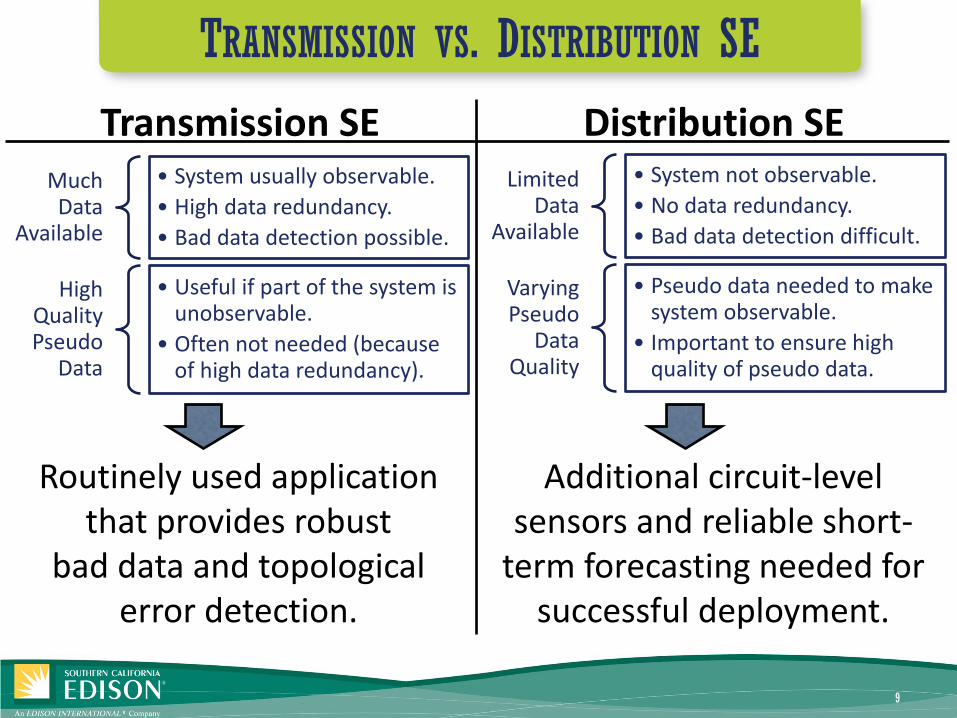
TRANSMISSION VS. DISTRIBUTION SE

9

Transmission SEMuch Data

Available

• System usually observable.

• High data redundancy.

• Bad data detection possible.

High Quality Pseudo

Data

• Useful if part of the system is unobservable.

• Often not needed (because of high data redundancy).

Distribution SELimited

Data Available

• System not observable.

• No data redundancy.

• Bad data detection difficult.

Varying Pseudo

Data Quality

• Pseudo data needed to make system observable.

• Important to ensure high quality of pseudo data.

Routinely used application that provides robust

bad data and topological error detection.

Additional circuit-level sensors and reliable short-

term forecasting needed for successful deployment.

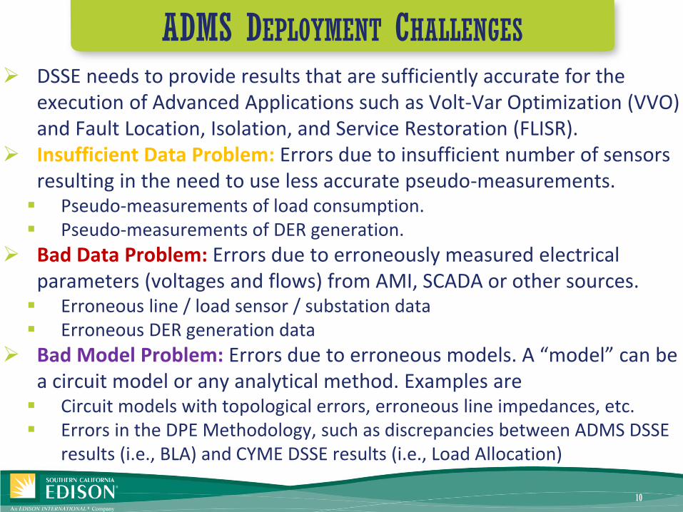
➢ DSSE needs to provide results that are sufficiently accurate for the execution of Advanced Applications such as Volt-Var Optimization (VVO) and Fault Location, Isolation, and Service Restoration (FLISR).

➢ Insufficient Data Problem: Errors due to insufficient number of sensors resulting in the need to use less accurate pseudo-measurements. ▪ Pseudo-measurements of load consumption.▪ Pseudo-measurements of DER generation.

➢ Bad Data Problem: Errors due to erroneously measured electrical parameters (voltages and flows) from AMI, SCADA or other sources. ▪ Erroneous line / load sensor / substation data▪ Erroneous DER generation data

➢ Bad Model Problem: Errors due to erroneous models. A “model” can be a circuit model or any analytical method. Examples are▪ Circuit models with topological errors, erroneous line impedances, etc.▪ Errors in the DPE Methodology, such as discrepancies between ADMS DSSE

results (i.e., BLA) and CYME DSSE results (i.e., Load Allocation)

ADMS DEPLOYMENT CHALLENGES

10

ADMS ERROR SOURCES

11

Insufficient Data Bad ModelBad Data

DSSE PERFORMANCE EVALUATION (DPE)

12

Planning ObjectiveDevelop Hardware & Software Requirements to achieve DSSE accuracy needed to run all Advanced Applications

optimally and violation-free.

Adding telemetry

points to fix Insufficient

Data problem –how many are needed and optimal locations?

How often should the

DSSE be executed?

Optimal use of data from line sensors, Large

Customer Metering, Short

Term Forecasting &

Residential AMI?

Are P & Q data needed or is measuring

current magnitude enough?

Operational ObjectiveDevelop Operational Requirements to

maintain adequate DSSE accuracy under all conditions while running Advanced

Applications.

What is the impact of

o measurement errors (Bad Data)?

o topological errors (Bad Model)?

o DER and disrupting technologies such as Smart Inverters, storage, etc. (Bad Data, Bad Model)?

How can the operator tell if DSSE solution

can be trusted?

➢ Developed DPE Methodology to achieve planning and operational objectives.

➢ DPE Methodology & Tool are simulation based.▪ AMI / SCADA / PV Performance Data to create pseudo-

measurements and mimic real-time data.▪ CYME circuit simulation to mimic real-world. ▪ CYME circuit simulation to mimic ADMS behavior.

➢ Methodology agnostic to state estimation algorithm.▪ We use CYME’s load allocation as this method is similar

to the state estimation algorithm in our ADMS.▪ Other state estimation algorithms, such as CYME’s

DSSE module, can be used instead.

DSSE PERFORMANCE EVALUATION (DPE)

13

14

DSSE Performance Evaluation:

Planning Mode - Overview

OBJECTIVE OF DPE TOOL’S PLANNING MODE

15

o Planning Model geared towards improving ADMS’s ‘Insufficient Data’ problem.

o Informs sensor locations and STFE requirements to surgically improve ADMS accuracy.

o Assumes good sensor data and circuit model.


DPE TOOL – OVERVIEW OF PLANNING MODE

16


17


Planning Mode - Concept

DPE: CONCEPT

18

Monte Carlo Analysis

Determines a Risk by quantifying accuracies of DSSE estimates.

a Risk

Likelihood of DSSE reporting a violation when there is none.

DPE: CONCEPT

19

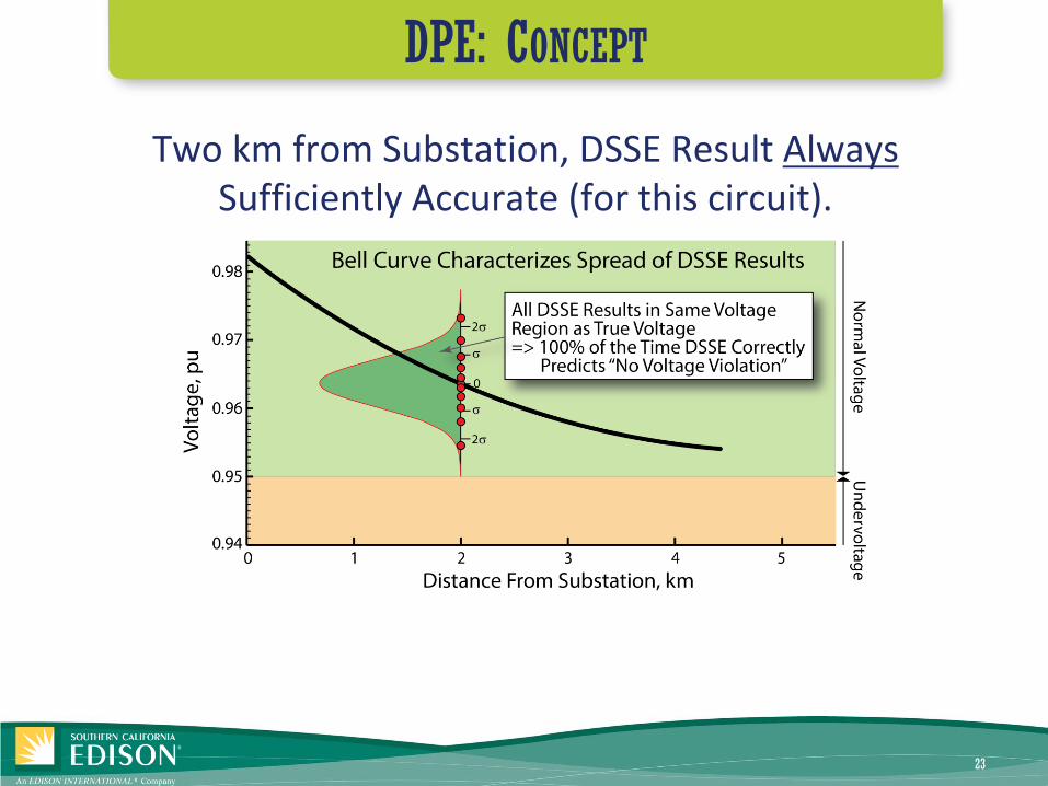
Premise: DSSE results are sufficiently accurate if they correctly identify compliances and violations.

Example: DSSE correctly reports ‘no undervoltage violation’.

DPE: CONCEPT

20

Premise: DSSE results are sufficiently accurate if they correctly identify compliances and violations.

Example: DSSE incorrectly reports ‘undervoltage violation’.

DPE: CONCEPT

21

Running DSSE Once

DPE: CONCEPT

22

Running DSSE Multiple Times (Monte Carlo Analysis)

DPE: CONCEPT

23

Two km from Substation, DSSE Result AlwaysSufficiently Accurate (for this circuit).

DPE: CONCEPT

24

At End of Circuit, DSSE Result Sometimes(15.85% in this Example) Not Accurate Enough.

a Risk: The risk of the DSSE giving false positives with regards to identifying voltage and flow violations

25


Planning Mode -Implementation

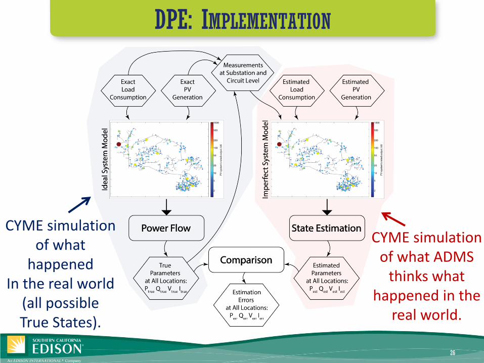
DPE: IMPLEMENTATION

26

CYME simulation of what

happenedIn the real world

(all possibleTrue States).

CYME simulation of what ADMS

thinks what happened in the

real world.

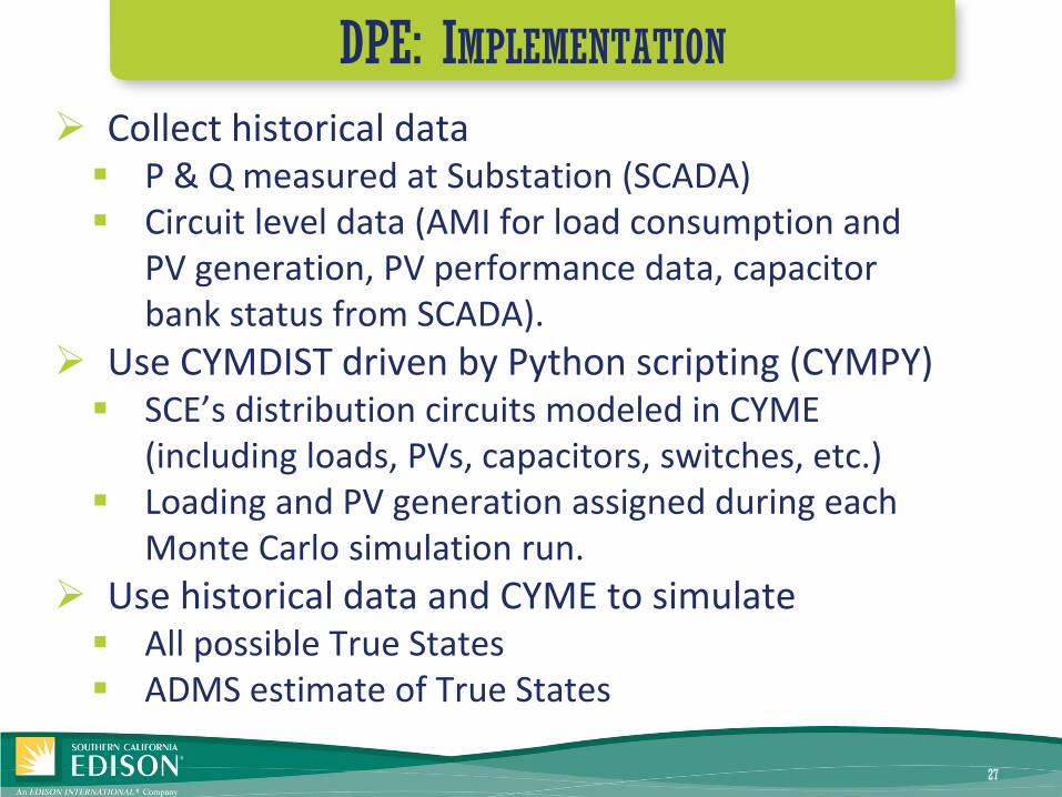
➢ Collect historical data▪ P & Q measured at Substation (SCADA)▪ Circuit level data (AMI for load consumption and

PV generation, PV performance data, capacitor bank status from SCADA).

➢ Use CYMDIST driven by Python scripting (CYMPY)▪ SCE’s distribution circuits modeled in CYME

(including loads, PVs, capacitors, switches, etc.)▪ Loading and PV generation assigned during each

Monte Carlo simulation run.

➢ Use historical data and CYME to simulate▪ All possible True States▪ ADMS estimate of True States

DPE: IMPLEMENTATION

27

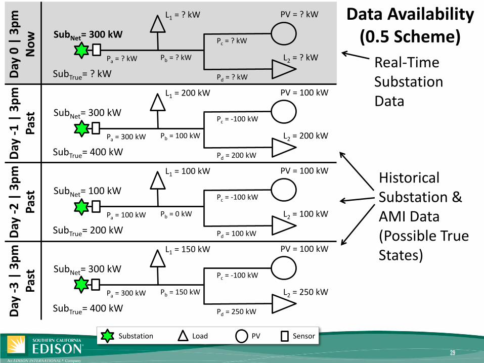
➢ CYME simulations of all loading scenarios that can happen based on historical data. These are our possible True States.

➢ Premise: What happened in the past can happen in the now.

➢ In other words▪ Use historical AMI data to capture loading scenarios that

are possible during time of ADMS execution.▪ Realistically captures load variation and correlation

between individual loads.

CYME SIMULATION OF TRUE STATES

28

29

Substation Load PV Sensor

L1 = 150 kW

SubNet= 300 kW

L2 = 250 kW

PV = 100 kW

Pb = 150 kWPa = 300 kW

Pd = 250 kW

Pc = -100 kW

SubTrue= 400 kW

L1 = 100 kW

SubNet= 100 kW

L2 = 100 kW

PV = 100 kW

Pb = 0 kWPa = 100 kW

Pd = 100 kW

Pc = -100 kW

SubTrue= 200 kW

L1 = 200 kW

SubNet= 300 kW

L2 = 200 kW

PV = 100 kW

Pb = 100 kWPa = 300 kW

Pd = 200 kW

Pc = -100 kW

SubTrue= 400 kW

L1 = ? kW

SubNet= 300 kW

L2 = ? kW

PV = ? kW

Pb = ? kWPa = ? kW

Pd = ? kW

Pc = ? kW

SubTrue= ? kWDay

0 |

3p

mN

ow

Day

-1

| 3

pm

Pas

tD

ay -

2 |

3p

mP

ast

Day

-3

| 3

pm

Pas

tData Availability

(0.5 Scheme)

Real-Time Substation Data

Historical Substation & AMI Data (Possible True States)

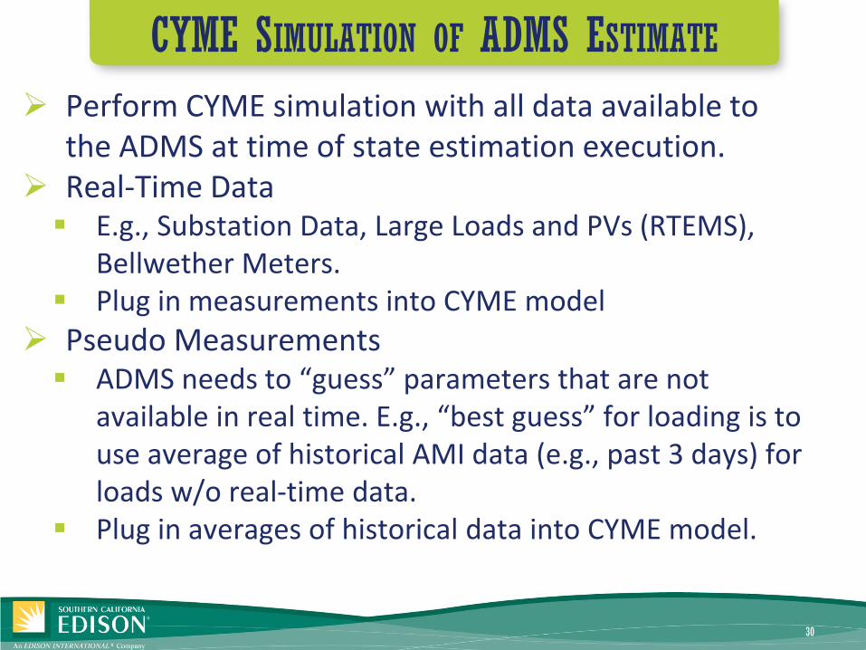
➢ Perform CYME simulation with all data available to the ADMS at time of state estimation execution.

➢ Real-Time Data▪ E.g., Substation Data, Large Loads and PVs (RTEMS),

Bellwether Meters.▪ Plug in measurements into CYME model

➢ Pseudo Measurements▪ ADMS needs to “guess” parameters that are not

available in real time. E.g., “best guess” for loading is to use average of historical AMI data (e.g., past 3 days) for loads w/o real-time data.

▪ Plug in averages of historical data into CYME model.

CYME SIMULATION OF ADMS ESTIMATE

30

31


L1 = 150 kW

SubNet= 300 kW

L2 = 250 kW

PV = 100 kW

Pb = 150 kWPa = 300 kW

Pd = 250 kW

Pc = -100 kW

SubTrue= 400 kW

L1 = 100 kW

SubNet= 100 kW

L2 = 100 kW

PV = 100 kW


Pd = 100 kW

Pc = -100 kW

SubTrue= 200 kW

L1 = 200 kW

SubNet= 300 kW

L2 = 200 kW

PV = 100 kW

Pb = 100 kWPa = 300 kW

Pd = 200 kW

Pc = -100 kW

SubTrue= 400 kW

L1p = (200+100+150)/3 = 150 kw

SubNet= 300 kW

L2p = 183 kW

PV = 100 kW

Pb = ? kWPa = ? kW

Pd = ? kW

Pc = ? kW

SubTrue= ?Day

0 |

3p

mN

ow

Day

-1

| 3

pm

Pas

tD

ay -

2 |

3p

mP

ast

Day

-3

| 3

pm

Pas

tPseudo

MeasurementsUse Historical Data for Pseudo Measurements

𝑳𝟏𝒑 =𝟐𝟎𝟎 + 𝟏𝟎𝟎 + 𝟏𝟓𝟎

𝟑𝒌𝑾

= 𝟏𝟓𝟎 𝒌𝑾

𝑳𝟐𝒑 =𝟐𝟎𝟎 + 𝟏𝟎𝟎 + 𝟐𝟓𝟎

𝟑𝐤𝐖

= 𝟏𝟖𝟑 𝒌𝑾

𝑷𝑽 =𝟏𝟎𝟎 + 𝟏𝟎𝟎 + 𝟏𝟎𝟎

𝟑𝐤𝐖

= 𝟏𝟎𝟎 𝒌𝑾

𝑺𝒖𝒃𝑻𝒓𝒖𝒆 = 𝟑𝟎𝟎 + 𝟏𝟎𝟎 𝒌𝑾= 𝟒𝟎𝟎 𝒌𝑾

AMI DATA FOR INDIVIDUAL LOADS

32

Use historical sets of AMI data from days with

similar conditions.

Use averages of historical AMI data as

pseudo measurements (e.g., AMI Data from previous

3 days).

SUBSTATION DATA

33

Allocate true substation

loading measured at

time of ADMS execution to

individual loads.

Allocate true substation

loading measured at

time of ADMS execution to

pseudo measurements.

DPE TOOL AUTOMATES ANALYSIS

34


35

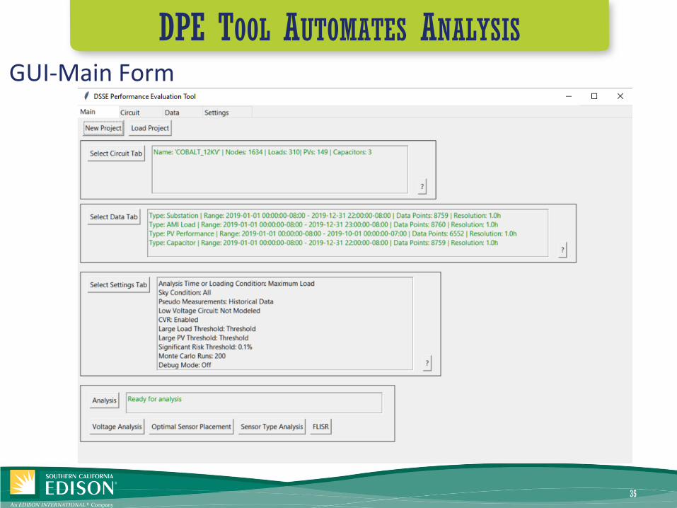
GUI-Main Form


36

GUI-Data Form


37

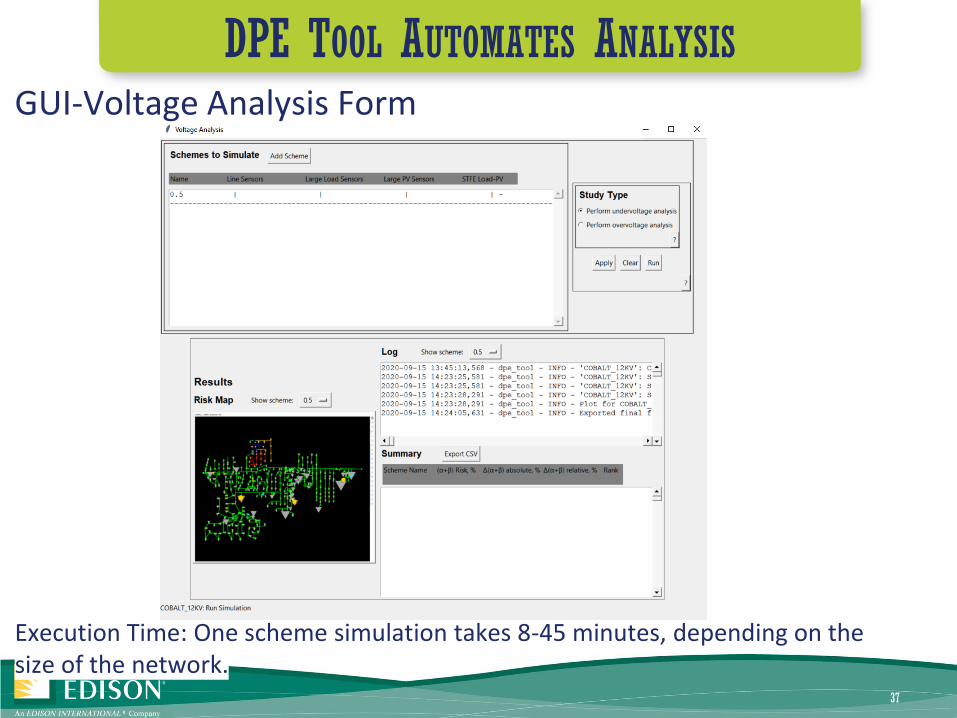
GUI-Voltage Analysis Form

Execution Time: One scheme simulation takes 8-45 minutes, depending on the size of the network.

38


Planning Mode - Functions

PLANNING MODE FUNCTIONS

39

Estimation-Improving Measures

Quantifies DSSE performance improvements achieved by operational forecasting and adding circuit-level sensors that provide a full measurement set (i.e., P & Q).

Sensor Type Analysis

Compares the DSSE performance achieved by P & Q line sensors and line sensors that measure ‘current magnitude only’.

DSSE Execution Interval Analysis

(Work In Progress)

Determines the maximum DSSE execution time interval that is needed to result in violation-free operation during normal operating conditions.

Optimal Sensor Placement Analysis

Identifies locations where placing a line sensor results in maximum DSSE performance improvement.

High PV Penetration

Perform analysis during clear-sky & cloudy-sky conditions when PV-caused voltage variability and DSSE estimation errors are largest.

40

DSSE Performance Evaluation: Planning Mode - Selected Results


41






(Work In Progress)




High PV Penetration


INVESTIGATED ESTIMATION-IMPROVING MEASURES

42

Estimation accuracy improved by additional sensors and operational forecasting (STFE). No Sensors on Circuit

(Base Case)• 0.5 Scheme: Substation Data Only

Automatic Switches w/ Sensors

• 1.5 / 2.5 / 3.5 Scheme: Substation Data + Data from One / Two / Three Circuit Locations

• Switch placement driven by provided reliability improvement (for now).

Operational Forecasting

• STFE10: Short-Term Forecast Engine improves operational load forecast from +-30% to +-10%

• STFE20: Short-Term Forecast Engine improves operational load forecast from +-30% to +-20%

HR Scheme • Place sensors near high α risk areas.

LL Scheme• Place sensors at large loads. This scheme simulates SCE’s deployment of

Real-Time Energy Meters (RTEMs), which monitor loads ≥200 kW capacity.

Combination Scheme • 1.5+ Scheme: 1.5 Scheme + HR Scheme + LL Scheme

ALPHA RISK ANALYSIS FOR UNDERVOLTAGE (VVO)

43

Quantified DSSE performance achieved by sensors and operational forecasting for seven circuits.

α risk = 0% 0% < α risk ≤ 3% 3% < α risk ≤ 10% α > 10%

Low PVPenetration

Circuits

High PVPenetration

Circuit

SOME OBSERVATIONS

44

➢ Combination Scheme needed to reduce α risk to near zero for all circuits.

➢ Large Load Sensor Scheme is most effective individual measure for reducing α risks on circuits with high portion of large loads (industrial/commercial).

➢ Main Line Sensor Schemes (1.5 / 2.5 / 3.5) improve α risk in most cases. Some ineffectiveness because α risk reduction is not a criterion for sensor placements (reliability is).

➢ Short-Term Forecasting Engine provides consistent reductions of α risks. Effectiveness highly dependent on forecast accuracy.

➢ High Risk Sensor Scheme can potentially provide high reduction of α risk, but has some implementation challenges.


45






(Work In Progress)




High PV Penetration


HIGH PV PENETRATION CIRCUIT

46

• One 250 kVA PV• 468 Residential PVs• 32% PV Penetration1

1 PV Penetration calculated as the ratio between aggregate PV Capacity and aggregate load rating x 100.

High Risk area locations and sensor placement requirements depend on sky condition.

HIGH PV PENETRATION CIRCUIT

47

Clear Sky

ScatteredClouds

High Risk Area (HR)Max risk=6.5%

Overcast(No PV Production)

RANKING OF MEASURES – CLEAR SKY

48

Rank 15.9% a+b Risk Reduction

•STFE10Short-Term Forecast Engine improves load and PV forecast to +-10%.


•STFE20Short-Term Forecast Engine improves load and PV forecast to +-20%.


(1.9% per sensor)

• HR Scheme with one additional sensorPlace a sensor near area with high risk.

Rank 4≈51.7% a+b Risk Reduction

(0.003% per sensor)

•PV Scheme Place sensors at all PVs.

Rank 4≈51.7% a+b Risk Reduction

(0.85% per sensor)

•2.5 Scheme Place two sensors on main line.


(1.0% per sensor)

•1.5 Scheme Place one sensor on main line.


(0.03% per sensor)

•LL SchemePlace sensors at large loads.

Rank 8-0.5% a+b Risk Reduction

(-0.5% per sensor)

•LPV Scheme Place sensors at Large PVs.

Short-Term Forecasting Engine most effective measure (also the case for cloudy sky conditions). Residential PV adds broad uncertainty. => Measures that broadly improve accuracy are most effective.

49

DSSE Performance Evaluation: Operational Mode

ADMS ERROR SOURCES

50


OBJECTIVE OF DPE TOOL’S OPERATIONAL MODE

51

o Operational Model geared towards improving ADMS’s ‘Bad Data’ and ‘Bad Model’ problems.

o Informs operator on quality of ADMS solution.o Identifies troubled circuit locations (high

inconsistency) that can possibly be improved by deploying additional sensors.


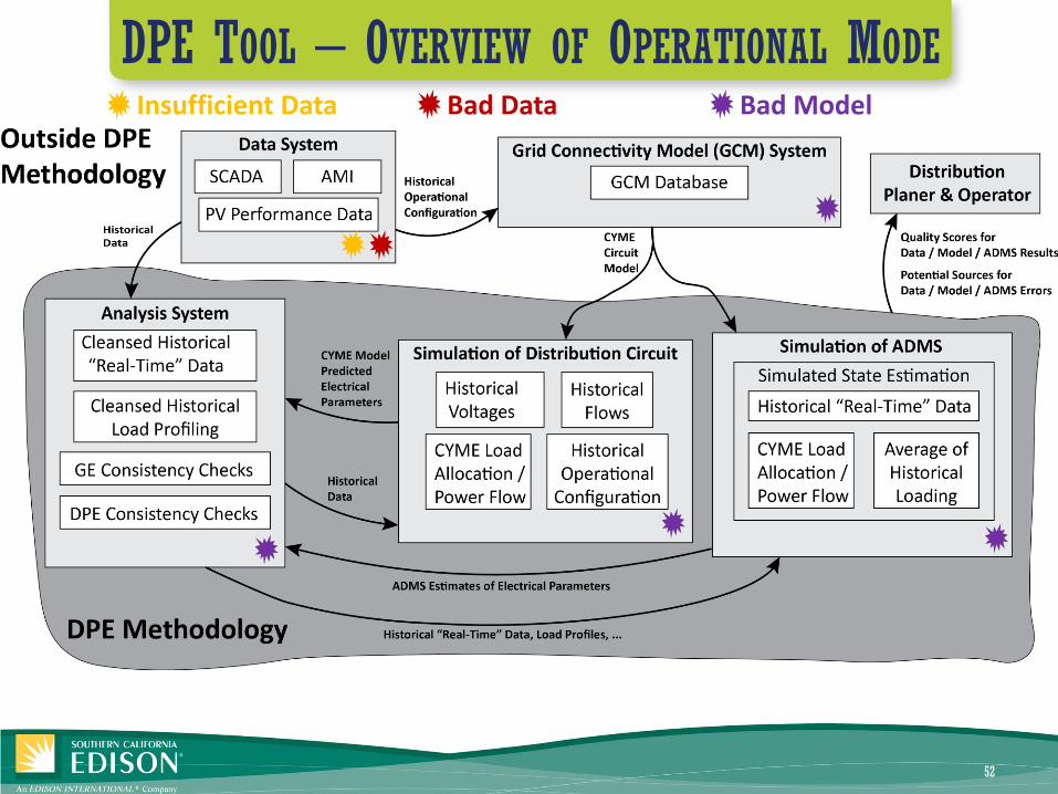
DPE TOOL – OVERVIEW OF OPERATIONAL MODE

52


Comparison

Quality of Circuit Model and Field Data

Circuit SimulationsLoading based on feeder-head P&Q data and either

• AMI data for time of analysis or

• Historical averages of loading (load profiles)

Field Data

• P&Q and voltage from automated switches

• Current from RFIs

• Voltages from AMIs and capacitors

BENCHMARKING ADMS PERFORMANCE

53

➢ Deterministic simulations.➢ Use historical data as proxy for real-time data.➢ Comparison of Model-Predicted Voltages and Flows with

Field Data.➢ Use some line sensors measurements in simulation to

determine ▪ impact on flow and voltage mismatches.▪ ability to pinpoint error sources.

➢ Informs (1) quality of ADMS results and (2) quality of DPE Tool’s sensor deployment recommendations.

➢ Work in progress.

BENCHMARKING ADMS PERFORMANCE

54

55

Summary & Next Steps

DSSE PERFORMANCE EVALUATION METHODOLOGY

56

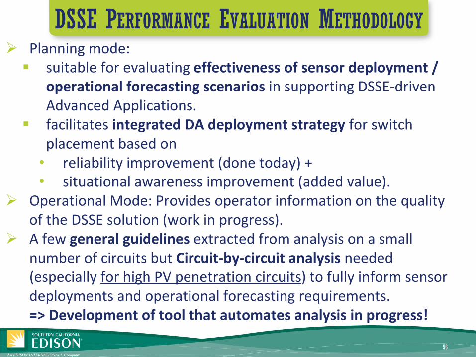
➢ Planning mode: ▪ suitable for evaluating effectiveness of sensor deployment /

operational forecasting scenarios in supporting DSSE-driven Advanced Applications.

▪ facilitates integrated DA deployment strategy for switch placement based on • reliability improvement (done today) +• situational awareness improvement (added value).

➢ Operational Mode: Provides operator information on the quality of the DSSE solution (work in progress).

➢ A few general guidelines extracted from analysis on a small number of circuits but Circuit-by-circuit analysis needed (especially for high PV penetration circuits) to fully inform sensor deployments and operational forecasting requirements. => Development of tool that automates analysis in progress!

Q & A

57

Thank you!

Muhammad Humayun

[email protected]

Jens [email protected]

mailto:[email protected]

mailto:[email protected]

58

Applications that rely on DSSEBasic and Advanced Applications

BASIC APPLICATIONS FOR DSSE

➢ Distribution System State Estimation (DSSE) is a Foundational Application that provides situational awareness and DER Visibility.▪ For instance, when a feeder is energized, inverter based

generation will be offline for 5 minutes after re-energization. The operator needs visibility into inverter performance to avoid overloads, overvoltages, and undervoltages during switching.

➢ DSSE informs optimization and control decisions of Grid Management System (GMS) Advanced Applications. ▪ For instance, DER can be dispatched to mitigate

overloads instead of building new infrastructure (aka non-wire alternatives).

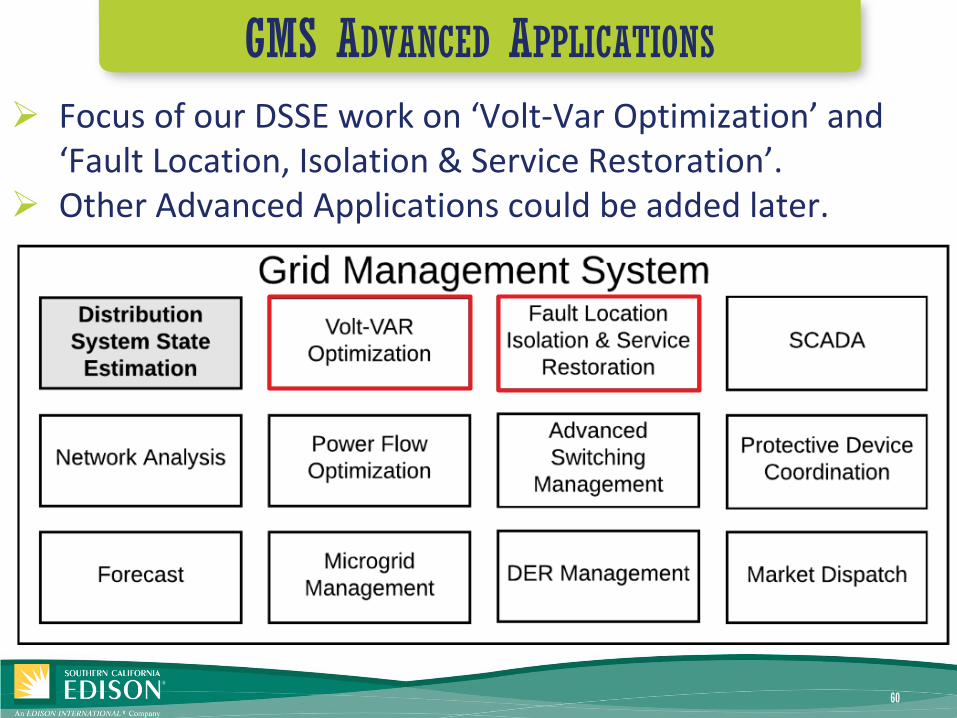
GMS ADVANCED APPLICATIONS

60

➢ Focus of our DSSE work on ‘Volt-Var Optimization’ and ‘Fault Location, Isolation & Service Restoration’.

➢ Other Advanced Applications could be added later.

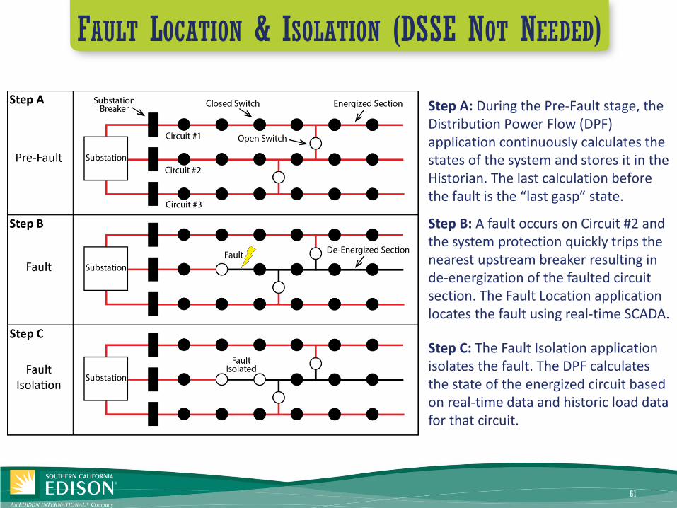
Step A: During the Pre-Fault stage, the Distribution Power Flow (DPF) application continuously calculates the states of the system and stores it in the Historian. The last calculation before the fault is the “last gasp” state.

FAULT LOCATION & ISOLATION (DSSE NOT NEEDED)

61

Step B: A fault occurs on Circuit #2 and the system protection quickly trips the nearest upstream breaker resulting in de-energization of the faulted circuit section. The Fault Location application locates the fault using real-time SCADA.

Step C: The Fault Isolation application isolates the fault. The DPF calculates the state of the energized circuit based on real-time data and historic load data for that circuit.

Steps D, E, & F: The Service Restoration (SR) application evaluates a number of ‘what if’ scenarios for service restoration. The evaluation comprises (1) determining a Switching Request that results in a circuit configuration that provides the optimal solution based on pre-specified optimization criteria and (2) ensuring that no violations occur during and after the execution of the Switching Request. Execution of the Protection Validation (PRV) application in study mode will ensure that the protective settings are valid for the new configuration. Execution of the Load Voltage Management (LVM) application in study mode to determine voltage control settings that avoid voltage problems.

GE’S SERVICE RESTORATION (DSSE NEEDED)

62

ALPHA RISK FOR OVERLOADING – GUIDELINES

63

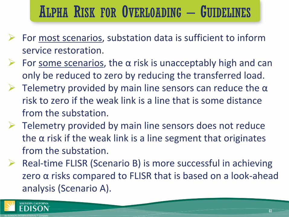
➢ For most scenarios, substation data is sufficient to inform service restoration.

➢ For some scenarios, the α risk is unacceptably high and can only be reduced to zero by reducing the transferred load.

➢ Telemetry provided by main line sensors can reduce the α risk to zero if the weak link is a line that is some distance from the substation.

➢ Telemetry provided by main line sensors does not reduce the α risk if the weak link is a line segment that originates from the substation.

➢ Real-time FLISR (Scenario B) is more successful in achieving zero α risks compared to FLISR that is based on a look-ahead analysis (Scenario A).

64

DSSE Evaluation WorkMethodology

Example for simple circuit presented in next slides➢ ADMS process to estimate loads▪ Used in the ADMS and replicated in our simulations. ▪ Simple circuit with two loads and one PV. Ignore losses.▪ Clear-sky (i.e., predictable) PV generation.▪ 0.5 Scheme (substation data available in real-time).▪ Detailed cloudy-sky scenario in Phase III report.

➢ Possible true states of loads▪ Simple circuit with historical data from three days prior to

ADMS execution (used as possible true states in stochastic analysis to evaluate ADMS estimates).

▪ Filter out prior days with substation loading that is very different from the one at time of ADMS execution (addressing Josh’s concern).

SIMPLE EXAMPLE

65

66

This is what the ADMS is doing…

67


L1 = 150 kW

SubNet= 300 kW

L2 = 250 kW

PV = 100 kW

Pb = 150 kWPa = 300 kW

Pd = 250 kW

Pc = -100 kW

SubTrue= 400 kW

L1 = 100 kW

SubNet= 100 kW

L2 = 100 kW

PV = 100 kW


Pd = 100 kW

Pc = -100 kW

SubTrue= 200 kW

L1 = 200 kW

SubNet= 300 kW

L2 = 200 kW

PV = 100 kW

Pb = 100 kWPa = 300 kW

Pd = 200 kW

Pc = -100 kW

SubTrue= 400 kW

L1 = ? kW

SubNet= 300 kW

L2 = ? kW

PV = ? kW

Pb = ? kWPa = ? kW

Pd = ? kW

Pc = ? kW

SubTrue= ? kWDay

0 |

3p

mN

ow

Day

-1

| 3

pm

Pas

tD

ay -

2 |

3p

mP

ast

Day

-3

| 3

pm

Pas

tData Availability

(0.5 Scheme)

Real-Time Substation Data

Historical Substation & AMI Data

68


L1 = 150 kW

SubNet= 300 kW

L2 = 250 kW

PV = 100 kW

Pb = 150 kWPa = 300 kW

Pd = 250 kW

Pc = -100 kW

SubTrue= 400 kW

L1 = 100 kW

SubNet= 100 kW

L2 = 100 kW

PV = 100 kW


Pd = 100 kW

Pc = -100 kW

SubTrue= 200 kW

L1 = 200 kW

SubNet= 300 kW

L2 = 200 kW

PV = 100 kW

Pb = 100 kWPa = 300 kW

Pd = 200 kW

Pc = -100 kW

SubTrue= 400 kW

L1p = (200+100+150)/3 = 150 kw

SubNet= 300 kW

L2p = 183 kW

PV = 100 kW

Pb = ? kWPa = ? kW

Pd = ? kW

Pc = ? kW

SubTrue= ?Day

0 |

3p

mN

ow

Day

-1

| 3

pm

Pas

tD

ay -

2 |

3p

mP

ast

Day

-3

| 3

pm

Pas

tPseudo

MeasurementsUse Historical Data for Pseudo Measurements

𝑳𝟏𝒑 =𝟐𝟎𝟎 + 𝟏𝟎𝟎 + 𝟏𝟓𝟎

𝟑𝒌𝑾

= 𝟏𝟓𝟎 𝒌𝑾

𝑳𝟐𝒑 =𝟐𝟎𝟎 + 𝟏𝟎𝟎 + 𝟐𝟓𝟎

𝟑𝐤𝐖

= 𝟏𝟖𝟑 𝒌𝑾

𝑷𝑽 =𝟏𝟎𝟎 + 𝟏𝟎𝟎 + 𝟏𝟎𝟎

𝟑𝐤𝐖

= 𝟏𝟎𝟎 𝒌𝑾

𝑺𝒖𝒃𝑻𝒓𝒖𝒆 = 𝟑𝟎𝟎 + 𝟏𝟎𝟎 𝒌𝑾= 𝟒𝟎𝟎 𝒌𝑾

69


L1 = 150 kW

SubNet= 300 kW

L2 = 250 kW

PV = 100 kW

Pb = 150 kWPa = 300 kW

Pd = 250 kW

Pc = -100 kW

SubTrue= 400 kW

L1 = 100 kW

SubNet= 100 kW

L2 = 100 kW

PV = 100 kW


Pd = 100 kW

Pc = -100 kW

SubTrue= 200 kW

L1 = 200 kW

SubNet= 300 kW

L2 = 200 kW

PV = 100 kW

Pb = 100 kWPa = 300 kW

Pd = 200 kW

Pc = -100 kW

SubTrue= 400 kW

L1p = 150 kw

SubNet= 300 kW

L2p = 183 kW

PV = 100 kW

Pb = ? kWPa = ? kW

Pd = ? kW

Pc = ? kW

SubTrue= 400 kWDay

0 |

3p

mN

ow

Day

-1

| 3

pm

Pas

tD

ay -

2 |

3p

mP

ast

Day

-3

| 3

pm

Pas

tTrue Load

Use Real-Time Data and PV Pseudo Measurement to Calculate True Substation Load

𝑺𝒖𝒃𝑻𝒓𝒖𝒆 = (300 + 100) kW= 𝟒𝟎𝟎 𝒌𝑾

70


L1 = 150 kW

SubNet= 300 kW

L2 = 250 kW

PV = 100 kW

Pb = 150 kWPa = 300 kW

Pd = 250 kW

Pc = -100 kW

SubTrue= 400 kW

L1 = 100 kW

SubNet= 100 kW

L2 = 100 kW

PV = 100 kW


Pd = 100 kW

Pc = -100 kW

SubTrue= 200 kW

L1 = 200 kW

SubNet= 300 kW

L2 = 200 kW

PV = 100 kW

Pb = 100 kWPa = 300 kW

Pd = 200 kW

Pc = -100 kW

SubTrue= 400 kW

L1p = 150 kW

SubNet= 300 kW

L2p = 183 kW

PV = 100 kW

Pb = ? kWPa = ? kW

Pd = ? kW

Pc = ? kW

SubTrue= 400 kWDay

0 |

3p

mN

ow

Day

-1

| 3

pm

Pas

tD

ay -

2 |

3p

mP

ast

Day

-3

| 3

pm

Pas

tNeed for Load

Allocation

SubTrue and L1p + L2p

do not match.

L1p and L2p need to be scaled to match substation loading (i.e., perform load allocation)

𝑺𝒖𝒃𝑻𝒓𝒖𝒆 = 𝟒𝟎𝟎 𝒌𝑾

𝑳𝟏𝒑 + 𝑳𝟐𝒑 = 𝟏𝟓𝟎 + 𝟏𝟖𝟑 𝒌𝑾

= 𝟑𝟑𝟑 𝒌𝑾

71


L1 = 150 kW

SubNet= 300 kW

L2 = 250 kW

PV = 100 kW

Pb = 150 kWPa = 300 kW

Pd = 250 kW

Pc = -100 kW

SubTrue= 400 kW

L1 = 100 kW

SubNet= 100 kW

L2 = 100 kW

PV = 100 kW


Pd = 100 kW

Pc = -100 kW

SubTrue= 200 kW

L1 = 200 kW

SubNet= 300 kW

L2 = 200 kW

PV = 100 kW

Pb = 100 kWPa = 300 kW

Pd = 200 kW

Pc = -100 kW

SubTrue= 400 kW

L1 = 180 kw

SubNet= 300 kW

L2 = 220 kW

PV = 100 kW

Pb = 120 kWPa = 300 kW

Pd = 220 kW

Pc = 100 kW

SubTrue= 400 kWDay

0 |

3p

mN

ow

Day

-1

| 3

pm

Pas

tD

ay -

2 |

3p

mP

ast

Day

-3

| 3

pm

Pas

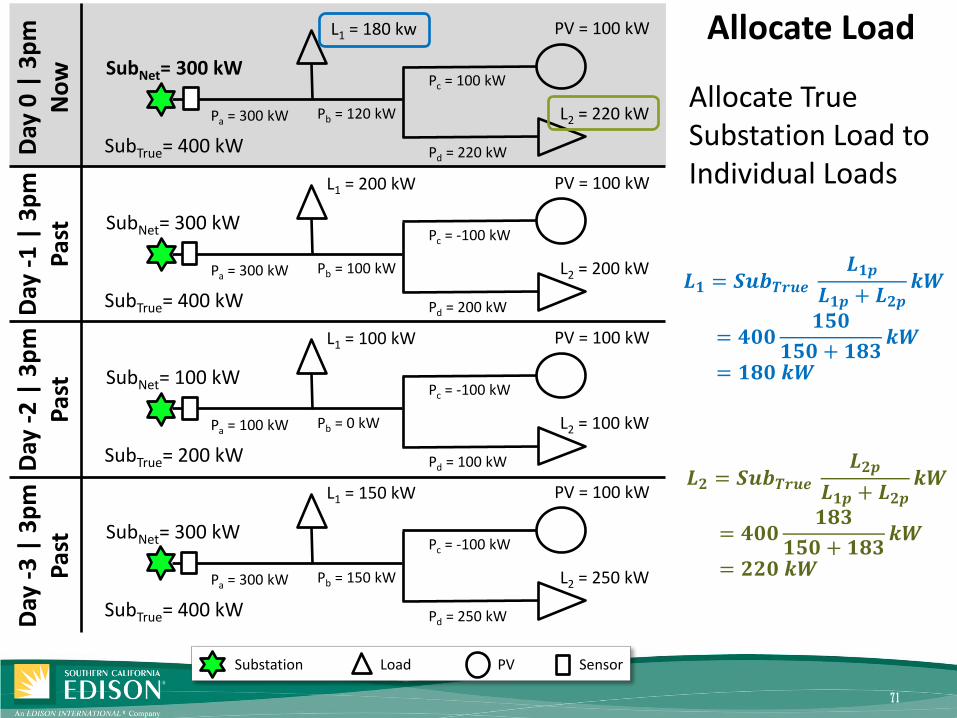
tAllocate Load

Allocate True Substation Load to Individual Loads

𝑳𝟏 = 𝑺𝒖𝒃𝑻𝒓𝒖𝒆𝑳𝟏𝒑

𝑳𝟏𝒑 + 𝑳𝟐𝒑𝒌𝑾

= 𝟒𝟎𝟎𝟏𝟓𝟎

𝟏𝟓𝟎 + 𝟏𝟖𝟑𝒌𝑾

= 𝟏𝟖𝟎 𝒌𝑾

𝑳𝟐 = 𝑺𝒖𝒃𝑻𝒓𝒖𝒆𝑳𝟐𝒑

𝑳𝟏𝒑 + 𝑳𝟐𝒑𝒌𝑾

= 𝟒𝟎𝟎𝟏𝟖𝟑

𝟏𝟓𝟎 + 𝟏𝟖𝟑𝒌𝑾

= 𝟐𝟐𝟎 𝒌𝑾

72

Question: How can we quantify the accuracy of this ADMS result?

L1 = 180 kw

SubNet= 300 kW

L2 = 220 kW

PV = 100 kW

Pb = 120 kWPa = 300 kW

Pd = 220 kW

Pc = 100 kW

SubTrue= 400 kW

Answer: Need to compare to possible true states…

73


L1 = 150 kW

SubNet= 300 kW

L2 = 250 kW

PV = 100 kW

Pb = 150 kWPa = 300 kW

Pd = 250 kW

Pc = -100 kW

SubTrue= 400 kW

L1 = 100 kW

SubNet= 100 kW

L2 = 100 kW

PV = 100 kW


Pd = 100 kW

Pc = -100 kW

SubTrue= 200 kW

L1 = 200 kW

SubNet= 300 kW

L2 = 200 kW

PV = 100 kW

Pb = 100 kWPa = 300 kW

Pd = 200 kW

Pc = -100 kW

SubTrue= 400 kW

L1 = 180 kw

SubNet= 300 kW

L2 = 220 kW

PV = 100 kW

Pb = 120 kWPa = 300 kW

Pd = 220 kW

Pc = 100 kW

SubTrue= 400 kWDay

0 |

3p

mN

ow

Day

-1

| 3

pm

Pas

tD

ay -

2 |

3p

mP

ast

Day

-3

| 3

pm

Pas

tPossible True

States

This is ADMS’s “best guess” of the loading but…

… loading at time of the ADMS execution could also be this…

… or this.

74


L1 = 150 kW

SubNet= 300 kW

L2 = 250 kW

PV = 100 kW

Pb = 150 kWPa = 300 kW

Pd = 250 kW

Pc = -100 kW

SubTrue= 400 kW

L1 = 100 kW

SubNet= 100 kW

L2 = 100 kW

PV = 100 kW


Pd = 100 kW

Pc = -100 kW

SubTrue= 200 kW

L1 = 200 kW

SubNet= 300 kW

L2 = 200 kW

PV = 100 kW

Pb = 100 kWPa = 300 kW

Pd = 200 kW

Pc = -100 kW

SubTrue= 400 kW

L1 = 180 kw

SubNet= 300 kW

L2 = 220 kW

PV = 100 kW

Pb = 120 kWPa = 300 kW

Pd = 220 kW

Pc = 100 kW

SubTrue= 400 kWDay

0 |

3p

mN

ow

Day

-1

| 3

pm

Pas

tD

ay -

2 |

3p

mP

ast

Day

-3

| 3

pm

Pas

tNot a Possible

True States

Exclude this loading scenario because substation data is much lower than it is at the time of ADMS execution.

75


L1 = 150 kW

SubNet= 300 kW

L2 = 250 kW

PV = 100 kW

Pb = 150 kWPa = 300 kW

Pd = 250 kW

Pc = -100 kW

SubTrue= 400 kW

L1 = 100 kW

SubNet= 100 kW

L2 = 100 kW

PV = 100 kW


Pd = 100 kW

Pc = -100 kW

SubTrue= 200 kW

L1 = 200 kW

SubNet= 300 kW

L2 = 200 kW

PV = 100 kW

Pb = 100 kWPa = 300 kW

Pd = 200 kW

Pc = -100 kW

SubTrue= 400 kW

L1 = 180 kw

SubNet= 300 kW

L2 = 220 kW

PV = 100 kW

Pb = 120 kWPa = 300 kW

Pd = 220 kW

Pc = 100 kW

SubTrue= 400 kWDay

0 |

3p

mN

ow

Day

-1

| 3

pm

Pas

tD

ay -

2 |

3p

mP

ast

Day

-3

| 3

pm

Pas

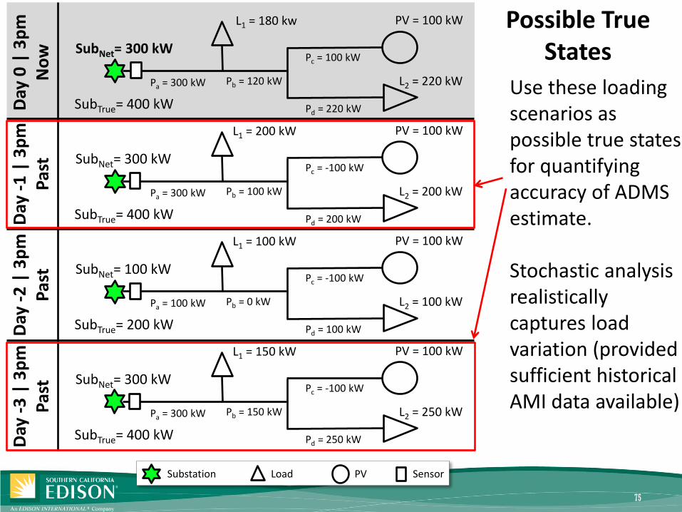
tPossible True

States

Use these loading scenarios as possible true states for quantifying accuracy of ADMS estimate.

Stochastic analysis realistically captures load variation (provided sufficient historical AMI data available)

d system state estimation (dsse) performance …

Documents