D-A36921 THEEFFECT OF TRUIIN NO TICES ON THE PRODUCTION OF I/JLFT ONAN AIRFOI U..U) A IR FORCE INST OF TECH

WRGHT-PATTERSON AFB OH SCHOOL OF ENGI.. K W TUPPERUNCLA SFIED DEC 83 AF OT/GAE/AA/83D-24 F/G 20/4 NL

l/immmmmmmmmmEEIIIIIEEEEIIIIEIIIIIIIIEIIIIIEmIIIIIIEEIIIIIE

IIIIIIIIIIIII

I

I.0 1_o1.II

1.25 1111.4 111.6

MICROCOPY RESOLUTION TEST CHARTNAN'ONIAL BLIRIAU Of S7ANDARDS-1963"A

.4*lI .

v .

Am,

..... ..

THE EFFECT OF TRAILING VORTICES ON THEPRODUCTION OF LIFT ON AN AIRFOILUNDERGOING A CONSTANT RATE OF

CHANGE OF ANGLE OF ATTACK

THESIS

Kenneth W. Tupper

Captain, USAF

AFIT/GAE/AA/83D-2 4

DEPARTMENT OF THE. AIR FORCEAIR Ut4ItSWY

^R FORCE INSTITUTE OFT

wW9t-fft** Air UfC W,*

84 01'1

AFIT/GAE/AA/83D-2 4

THE EFFECT OF TRAILING VORTICES ON THEPRODUCTION OF LIFT ON AN AIRFOILUNDERGOING A CONSTANT RATE OF

CHANGE OF ANGLE OF ATTACK

THESIS

Kenneth W. TupperCaptain, USAF

AFIT/GAE/AA/83D-2 4

DTICLECTEf

E

Approved for public release; distribution unlimited

AFIT/GAE/AA/83D-24

THE EFFECT OF TRAILING VORTICES ON THE PRODUCTION

OF LIFT ON AN AIRFOIL UNDERGOING A CONSTANT

RATE OF CHANGE OF ANGLE OF ATTACK

THESIS

Presented to the Faculty of the School of Engineering

of the Air Force Institute of Technology

Air University

In Partial Fulfillment of the

Requirements for the Degree of

Master of Science in Aeronautical Engineering

Acoession ForNTIS GRA&I

DTIC TABUnannoitin ceQdJustification:

Kenneth W. Tupper, B.S. By ----

Distribution/..Captain, USAF Availability Codes

I Avail and/orDist Special

December 1983

Approved for public release; distribution unlimited

1.9,.

Preface

- The purpose of this study was to investigate the effect

a trailing vortex wake has on an airfoil undjergoing a con-

stant rate of change of angle of attack, intwo-dimen-

sional, incompressible, irrotational flow. Potential flow

theory, conformal mapping by the Joukowski transformation,

and numerical integration and differentiation techniques were

used to develop a computer algorithm to model the problem.

Once the program was formulated, it was used to solve the

impulsive-start problem of airfoil motion. The results were

found to be in excellent agreement with the results obtained

by others. When applied to the constant rate-of-change of

angle-of-attack problem, the results showed that a trailing

vortex wake has a measurable and predictable effect on the

production of lift on an airfoil undergoing a constant

/he results of this work, taken alone, are helpful in

understanding the phenomena known as dynamic stall, bttt-'

coupled with existing boundary-layer studies the results

may lead to additional understanding of the phenomena. More

specifically, the computer program developed here could be

used to(more realistically predictthe inviscid flow about

a pitching airfoil as it approaches the dynamic-stall con-

ditions. -9

This study could never have been completed without the

help of others. I owe a great deal of thanks to Major Eric

Jumper, who not only posed this problem to me, but who also

ii

provided invaluable assistance throughout the investigation.

I also wish to thank Lt. Colonel Michael Smith for his help

with potential flow theory and his expert advise regarding

the writing of this report. Finally, I wish to thank my

wife Anneliese for her translations of the German references

and, most importantly, for her help in keeping the work in-

volved in this thesis in proper perspective.

Kenneth W. Tupper

S

iii

Table of Contents

Page

Preface .... ............ . .. . ........... .i

List of Figures . . . . . .................. v

List of Tables . . . . . . . . . . . . . . . . . . . .vii

Abstract . . . . . . . . . . . . . . . . . . . . . . . . viii

I. Introduction. . . . . .............. 1

II. Solution Development ....... ............... 3

Solution Overview ......................... 3Equations for Flow About a Cylinder . . . .. 5Joukowski Transformation ........ ...... 10Determination of Strength of Vortices 11Velocities Induced at Discrete Vorticesand on the Cylinder ............. .. 14Circulation About the Airfoil.... . ... 17Velocity in the Airfoil Frame .. . .. . 18Pressure, Lift, Vorticity Distributionon the Airfoil. ..... ............ ... 19Numerical Solution Process. ........... . 21

III. Results ............................. .. 25

Numerical Method Verification . . . 25Application to Constant-& Flow .......... ... 41

Selection of Standard StartingConditions. .......... 41General Effect of a on CI .. . . 47

Effect of Airfoil Thickness on aEffect. ........ 47Effect of Airfoil Camber'on a Effect. 50

IV. Conclusion . . . . . ............... . 54

V. Recommendation. o . . . . . . . . . .. 57

Appendix: Computer Program . . . . .. . . . . . .. 58

Bibliography . . . . . . o . . . . . . . . . . . .. 66

Vita . . . . . . . . . . . . . . . . . . . o. . . . . . 68

iv

WWT

List of FiQures

Figure Page1. Cylinder in Free Stream at Angle of Attack with

Vortex and Image. . . ............ . . . . 6

2. Planes of the Joukowski Transformation. . . . . . 12

3. Build-up of Circulation on an Impulsively-StartedFlat Plate . .. . . . ............ . . . 26

4. Build-up of C on an Impulsively-Started FlatPlate . . . . . . . . . . . . . . . . . . . . . . 27

5. Coefficient of Lift vs. Distance Traveled (Effectof At* on Numerical Solution) . . . . . . . . . . 29

6. Dimensionless Vorticity Distribution on a FlatPlate, a = 0.1 radians ................ 30

7. Pressure Difference Distribution on a Flat Plate,= 0.1 radians. . . . ............ . . . 31

8. Wake Vortex Sheet Roll-up for a Flat Plate,a= 0.1 radians ................. 33

9. Build-up of C£ on a 25.5% Thick Symmetric JoukowskiAirfoil . . . . ..................... 34

10. Wake Vortex Sheet Roll-up for a Flat Plate,a. = 100 (Predictor-Corrector vs. PresentMethod) . . . . . . . . . . . . . . . . . . .. . 36

11. Dimensionless Vorticity Distribution, 25.5% ThickSymmetric Joukowski Airfoil, a = 0.1 radians. . 39

12. Pressure Difference Distribution, 25.5% ThickSymmetric Joukowski Airfoil, a = 0.1 radians . . 40

13. Coefficient of Lift vs..Angle of Attack (Effectof Start Time to Begin a for ao = 0 ° ) . .. . 42

14. Coefficient of Lift vs. Angle of Attack (Effectof Start Time to Begin i for ao = 5 ) . . . .. . 44

15. Coefficient of Lift vs. Angle of Attack (Effectof Initial Angle.of Attack (C£ at 90% Steady-StateValue) to Begin a). . . . . . . . . . . . . . . . 45

v

<I _ _ _______

Figure Page

16. Coefficient of Lift vs. Angle of Attack (Effectof At* on Curve Slope) ..... ............ . . . 46

17. Coefficient of Lift vs. Angle of Attack (Effectsof a for 15% Thick Symmetric JoukowskiAirfoil) . . . . . . . . . . . . . . . . .. . 48

18. Coefficient of Lift vs. Angle of Attack (Slopeqhange as Angle of Attack Increases at Constanta) . . . . . . . . . . . . . . . . . . . . . . . . 49

19. Airfoil Thickness Effect on the Slope of the C2vs. a Curve for Constant d . . ............ 51

20. Airfoil Camber Effect.on the Slope of the C vs.aCurve for Constant a .... .............. ... 53

21. Flat Plate C Changes as a Function of a. . . . 55a

vi

-- _______• ,_ ._, .Mob"&-*

List of Tables

Table Page

I. Comparison of C Calculated by Simple PredictorMethod to C Caiculated by Predictor-CorrectorMethod. Flat Plate Airfoil, a = 10 . . . . . . 38

II. Comparison of C Calculated by Simple PredictorMethod to C Cafculated by Predictor-CorrectorMethod. Flit Plate Airfoil, a* = 0.035 . . . . 38

v

t ,. , - - r~ i •,,1.

AFIT/GAE/AA/83D-26

J4

Abstract

This study explored the effect of a trailing vortexti wake on the production of lift on an airfoil undergoing a

constant rate of change of angle of attack, a. The study

showed that when an airfoil encounters a constant-a flow,

the trailing vortex wake acts to suppress the slope of the

airfoil's C vs. a curve. The change in magnitude of this

effect as a function of airfoil thickness and camber was

also investigated.

Potential flow theory was used to model the flow about

a two-dimensional circular cylinder, and that flow was trans-

formed to flow about an airfoil by the Joukowski transforma-

tion. The trailing vortex wake was modeled by a sequence of

discrete point vortices, and the pitching motion of the air-

foil was modeled by a series of small incremental changes

in angle of attack, Aa, over a short period of time, At.

The rate of change of angle of attack, a, was then defined

as A(/At. After each time change At, a was changed by an

amount &a. A discrete vortex was introduced into the wake at

a distance U.At behind the airfoil trailing edge, and a

bound vortex of equal strength but opposite sense was intro-

duced to satisfy the Kutta condition and keep the total cir-

culation in the flow field equal to zero. As each new vor-

tex pair was introduced, all other trailing vortices were

viii

assumed to move in the wake by a distance UAt, where U is

the velocity induced at a vortex position by all other trail-

ing vortices, the bound vortices, and the free stream flow.

The unsteady Bernoulli equation was solved using numerical

integration and differentiation techniques to determine pres-

sure difference distribution, vorticity distribution, and

coefficient of lift on the airfoil for that instant in time.

This information was then used to investigate the overall

effect of constant- flow as well as the effect of thickness

and camber on the constant- problem, and simple rules for

predicting the effects were developed.

ix

fi_________________________t i ______________'________. ........__________ T --

THE EFFECT OF TRAILING VORTICES ON THE PRODUCTION

OF LIFT ON AN AIRFOIL UNDERGOING A CONSTANT

RATE OF CHANGE OF ANGLE OF ATTACK

I. Introduction

It has been determined experimentally that an airfoil

pitching at some rate of change of angle of attack a stalls

at a higher angle of attack a than the static stall a. Max

von Kramer first showed this with his experiments in 1932

(1), where he held the airfoil fixed in space and rotated

the flow over the airfoil to create an . Deekens and Kuebler

(2) and Daley (3) ran similar experiments for a constant a,

but rather than rotating the flow, they rotated the airfoil

in a constant velocity free stream to produce their a. In

all three cases the stall occurred at a higher angle of attack

than the static-stall angle of attack. However, because of

the different methods used to produce a, Kramer's results

showed a much smaller change in stall angle of attack than

did Deekens and Kuebler and Daley.

Following these experiments, attempts have been made to

analytically model the case of an airfoil undergoing a con-

stant . Docken (4) and Lawrence (5) have tackled the prob-

lem using a momentum integral method, but both assumed in

their solution that the effect of the trailing vortices in

o1

the airfoil wake was small and could be neglected. Thus,

they assumed that the inviscid flow velocity outside the

airfoil boundary layer at any angle of attack was that which

would exist in the steady state at that angle of attack. It

is the intent of this thesis to determine the validity of

that assumption by analyzing the effect a trailing vortex

wake has on the inviscid flow field about an airfoil under-

going a constant rate of change in angle of attack (i.e.,

constant a). The effect of the trailing vortex wake on the

flow about the airfoil can be analyzed by determining how

the vorticity distribution and pressure difference distribu-

tion on the airfoil develop under the influence of the

(taking the trailing wake into account), and by observing

the effect of the a on the C vs. a curve.

J

ii i2__ _ _ _ _ _ _ _ _ _ __ _ _ _ _ _ _ _ _ _ _ -

II. Solution Development

Solution Overview

Consider an airfoil at an angle of attack whi(l: under-

goes an impulsively started motion of velocity U Assume

* the airfoil is immersed in an incompressible, inviscid fluid.

Under these circumstances, a stagnation point of the flow

would occur on the upper surface of the airfoil. This would$

* imply an infinite velocity at the airfoil trailing edge. It

is known, however, that the flow at the trailing edge of such

an airfoil becomes smooth and has a finite velocity. This

is known as the Kutta condition. Imposing the Kutta condi-

tion requires the formation of circulation around the airfoil

to move the stagnation point to the trailing edge. This cir-

culation can be modeled as a vortex bound to the airfoil.

The total circulation in the flow must remain equal to zero

by Kelvin's theorem, and thus circulation in the opposite

sense is shed in the form of a discrete vortex into the air-

foil wake. The strength of this vortex is just equal and

opposite to that of the bound vortex on the airfoil. The

equal and opposite strengths of the bound and shed vortices

are just sufficient to satisfy the Kutta condition and

Kelvin's theorem.

Thus, when the airfoil at angle of attack is impulsively

* started, circulation about the airfoil develops, and a wake

vortex is shed. After a time At, this shed vortex is arbi-

trarily assumed to be at a distance U At from the trailing

3

T li l-

iV

edge (6:21). The bound vortex and shed vortex both affect

the flow about the airfoil, and their strengths are such

that the Kutta condition at the trailing edge is satisfied.

Knowing the strengths of these vortices, the instantaneous

values of circulation about the airfoil, as well as the

pressure difference distribution, vorticity distribution,

and coefficient of lift on the airfoil can be calculated.

After another time At, the shed vortex has moved further

downstream by a distance Usv At, where Usv is the velocity

at the shed vortex location imposed by the free stream and

all other vortices, including the bound vortex. In cases

other than the impulsive-start problem, the angle of attack

may also have changed by some amount equal to L~t, where

is the average rate-change of angle of attack over the

given time period At. The strength of the first shed vortex

remains fixed, and thus another bound vortex and shed vortex

must be introduced to keep the Kutta condition satisfied.

This second shed vortex is assumed to be at a distance

.U00t behind the trailing edge. The equal and opposite

strengths of these new bound and shed vortices are again de-

termined by imposing the Kutta condition. Now, for this new

instant in time, the instantaneous values of airfoil cir-

culation, pressure difference distribution, vorticity dis-

tribution, and coefficient of lift can once again be cal-

culated. This process can be repeated for any number of

discrete time steps At desired, and for that matter any

a(t), although in this study . was held constant. By

4

following this method, a time history of the development of

circulation, pressure difference distribution, vorticity

distribution, and coefficient of lift on the airfoil can be

observed.

Equations for Flow About a Cylinder

When solving a problem in two-dimensional incompressi-

ble, irrotational flow, it is often useful to make use of

conformal mapping. In this case, the problem is solved for

flow about a two-dimensional cylinder, then the Joukowski

transformation is used to find the solution for a Joukowski

airfoil.

Consider the flow of an incompressible, irrotational

fluid in the 0-plane. The flow is inclined at an angle a

to the x-axis (see Fig. 1). The stream function and poten-

tial function 0 for this flow are given by (7:245):

= U (Ycos a - X sina) ()

= U (X cos a + Y sin a) (2)

where U. is the magnitude of the free stream velocity.

If a doublet of strength K, axis inclined at angle a

to the X-axis, is placed at the origin of the o-plane, the

4 stream function 4' and potential function 0 are given by:

_K[Y cos aXs n (

2 + y2 (3)

5

MYY

<2(A, B r(0'7)

I ~U 0

p plane

Fig. 1. Cylinder in Free Stream at Angle ofAttack With Vortex and Image

6

* * II

0=K Xcos a + Y si a 4

2 2 1

2,rr x2 + y2 4

Since stream functions and potential functions are lin-

ear, they may be superimposed to create new flows. Therefore,

the stream and potential functions for" a doublet in a uniform

free stream at angle M to the X-axis can be written as:

P= U (Y cos a - X sin a) - Y cos a - X sin a

= (Y cos a - X sin 21 2 +2 (5)

= U (X cos a + Y sin a) + X cos a + Y sina2Tx2+ a]

= (X cos a + Y sin a) [U0 + K 1 (6)T X 2 + y2(

If strength K is such that K/2vUO = a2 , where a is the

radius of a cylinder, then the zero streamline will be the

line along which Y cos a = X sin a and the cylinder of

radius a , centered at the origin (8:89). The stream func-

tion and potential function are now:

42 [ a]V/ = U(Y cos a - X sin a) 1 2 2 (7)

0 = U (X cos a + Y sin a) 1 + 2 a 2 (8)

7

I .2

Next, consider a vortex of strength -T located at

( ,q) in the c-plane. If a vortex of strength r is placed

at point (A,B) such that (A,B) is the inverse point of

( ,1) about the surface of the cylinder of radius a, (i.e.,

If,7rj= 1/IA,BI ), then the surface of the cylinder remains astreamline by the circle theorem (9:84,85), and the total

circulation remains zero. The stream and potential functions

for a line vortex are given by (8:82)

=' n (r) (9)

-Trr-F (10)

where r is the distance from the vortex to the point in the

c-plane where 4 and 0 are evaluated, and e is the angle meas-

ured counterclockwise from the x-axis to r. Adding %P and 0

for each vortex in the pair yields

4'P 2-n [ ((X-A) 2 (Y-B))

- r In ((X-4) 2 + (Y-?7) 2) 1] (11)

r rr I X-AI7-arctanjl_-]_ E arctan [ (12)

Note that A = (/r') cos e', B = (1/r') sin e' , and since

cos e' = 4/r' , sin e' = 7/r' (see Fig. 1), then

A = 2 + 2 (13)

B= 2 2 (14)

4

8

After using the trigonometric identity (8:86)

arctan a - arctan 8 arctan a (15)

and performing some algebraic manipulation, one derives

r [ (X-A)2 + (Y-B) 2 (16)

I(x- V 2 + (Y - 11) 2

0 Xarctan -)(Y- - (X-A)(Y-71) (17)=2 rta I(Y-n) (Y-B) + (X-J) (X-A)

Finally, let there be N vortex pairs as just described.

Superimposing the N vortex pairs onto the cylinder in a

uniform free stream flow, the stream and potential functions

become:

= (Y cos a - X sin a) 2 a 2

N rXA) 2 + (Y-B) 2+ Z: " In (18)i=1 n[(X_)2 + (yn)2

2

0 = U.(X cos a + Y sin aL) 1 + a2

N+ i.[ (X-ti)(Y-Bi ) - (X-A i )(Y-n i

)

i=l i arctan (Y-i)(Y-Bi) + (X-i)(X-Ai) (19)

The velocity at any point (X,Y) in the flow field can

be obtained directly by differentiation and some algebraic

9

JA

manipulation of Eq. (18). The velocities in the X-direction

(U,) and the Y-direction (V are:

=-Ilk U. [Cos a cos a 2a 2Xy sin a 2 2y2 cos 1Sc X2 + y2 (X2 + y2)2 (X2 + y2)2

N ri Y-Bi Y-71i+ E 2,r2_ -2 2 (20)i=l t(X-Ai) 2+(Y-Bi)2 (X- i) +Y-1i ) 2

_- Tu [sin - a 2 sin a 2a2XY cos + 2a2X2 sin a0 a = X2 + Y2 (X 2 + y2)2 (X2 + y2)2

N i [ X-i_] (21)+ Tr (XAi)y (B )2il (X-_i2+Y-i)2 (XA 2+ 2B

The stream function V1, potential function 0, and general

velocities U0 and V0 for any point in the 0-plane are

now known.

Joukowski Transformation

The Joukowski transformation can be used to transform a

flow from a cylinder plane to an airfoil plane. We already

have the equations for the flow in the 0-plane, where the

cylinder is centered at the origin. In complex variable

form, the position of a point in the 0-plane can be expressed

as 0 = r e . We can transform this point to the o'-plane

by the transformation o' = oe' 8 + . (10:461). This ro-

tates points in the 0-plane 8 radians clockwise, and then

10

-

displaces them by an amount 4. The positive X-coordinate

crossed by the cylinder in the -plane, t , maps into the

point Ct ' (see Fig. 2). Transforming from the 0'-plane

to the Z-plane, the Joukowski transformation is used. It

is given by: , t, 2

Z = + t (22)

This transforms the cylinder in the 0'-plane to an airfoil

shape in the Z-plane. The point pt' maps to the trailing

edge of the airfoil shape in the Z-plane.

Determination of Strength of Vortices

Having seen how the Joukowski transformation maps a

cylinder in the 0-plane into an airfoil shape in the Z-plane,

it is time to relate the flows in the C and Z-planes. As

mentioned before, the solution involves placing discrete

vortices in the airfoil wake to simulate the vortex sheet

shed into the wake as circulation builds around the airfoil.

Images of these vortices are placed inside the cylinder to

simulate the airfoil bound vortex. The strength of each

vortex is determined by satisfying the Kutta condition at

each discrete time step. The Kutta condition implies that a

stagnation point of the flow is at the airfoil trailing edge.

As seen in the Joukowski transformation, the point Ot in

the O-plane maps into the trailing edge of the airfoil in the

Z-plane. Therefore, establishing a stagnation point at 0t

in the O-plane satisfies the Kutta condition in the Z-plane

(10:469).

I,.I

p -Plane P' -Plane

y

aa

Z -Plane

Fig. 2. Planes of the Joukowski Transformation

12

I' _ _ _ _ _ _ _ _ _ _ _ _ _ _ __*A_ _ _ _ _

To make t a stagnation point in the 0-plane, set the

velocity U. equal to zero at that point and solve for the

circulation strength ]-in Eq. (20). This value of F will

be the same in the Z-plane, for circulation is unchanged in

the Joukowski transformation (10:458). Taking Eq. (20) for

U, letting the cylinder radius a = 1 , and recalling that

X 2 + Y2 = 1 for points on a cylinder of radius a = 1 , one

arrives at:

2U 0 = U. cos a - cos a 2XY sin a + 2Y cos Ci

N fi[ Y-B Y-Y-i+ Z 2 2+- 2 - 1 (23)i=l -(XBA ()-+(Y - i B )- I

Let N = 1 to solve for the strength of the first shed vor-

tex. Solving for F /U., one gets:

r 2r (2XY sin a - 2 Cos a)U00 r Y-B Y- 7 - 24

(XA) 2+(YB)2 (X-)2+(y_7)I (24)

* Recalling the relations for A and B given by Eqs. (13) and

(14) and again making use of the fact that X2 + y2 = 1 on

the cylinder, Eq. (24) becomes

i 41T (X sin a - Y cos a)(4 2 + 72 + 1 - 2(Xt+Y7))( 2 5 )

U. t ~2 + 72 _1(5

Define r/u. as F*, the non-dimensional circulation, and

note that at at , X = 1 and Y = 0 . This changes Eq. (25)

to

13

4rr* 4i sin (42 + 12 + 1 - 24) (26)2 + ?12_1

When solving for each subsequent F term, all previous F*

terms are known. Thus, Eq. (23) can be solved for F

In general, then

4r sin ai (4i 2 + ni2 + 1 -2 i )

34i 2 + 7 - 1

i-i r+ 2 )E k 4k2 + 2 (27)k=l k 2 + nk 2+ 2 - 2 k

Velocities Induced at Discrete Vortices and on the Cylinder

For each time step taken, the strength of the vortex

pair introduced at that time step can now be calculated

using Eq. (27). However, from one time step to the next,

each vortex introduced in the wake moves away from the air-

foil some distance, that distance being equal to the velocity

at the position of the vortex times the time step, At •

The velocity at the position of each vortex depends upon not

only the free stream velocity, but also the velocities in-

duced at that position by all other vortices in the field.

Equations (20) and (21) can be used to find that velocity in

the 0-plane. Let ( m7m) be the coordinates of the posi-

tion at which the trailing vortex is located, the i sub-

script denote the time step at which the velocity is com-

puted, and the k subscript identify an individual vortex.

r 14

Solving equations (20) and (21) for the non-dimensional

U/U ,V/U , and recalling r = F/U ,one gets:

U 2

m CosOL . -Cos a. 2mmsna % CSO osiU. c0 2 + I2 4m2 + m2 2 4M2 + m2 )2

+ [r 17 I(m2 ) + m] (28)2 + 2--4- 2 + ?Im2)2 _ 2 -m 2 11m 2 + 1

+ *

k_ F 1, 1ky -B k-I-1kim 2i ( -mAk) 2+(Ym-Bk) 2 (4 nk) 2 +7m_,k) 2

k/r 2En 'm no a' +22s in k

VM = sin a. -sin i - 2i 2 iU0 m 2+m 2 ( m 2 + 4m2)2 {4m 2 + m2) 2

21 2 22

m 2 M 2 1) 1

- ( 2 + ? (29)

F*

N k [ k - k+ 2- 2+ 2 2 2k=l, 2T (km-4k) (07m-77k) ( km-A k ) +(77m-Bk)

k/m

15

Equations (28) and (29) describe the velocity that exists at

any vortex location (m P 7m ) as induced by the uniform

free stream and all other vortices in the flow field.

The velocity induced along the cylinder surface is

needed to determine the pressure distribution on the airfoil.

Again making use of the o-plane velocity equations (20) and

(21), and recalling that X2 + y2 = 1 on the cylinder in

the 0-plane, the non-dimensional velocities become:

U_ = -2XY sina +N r Y( 2+ 2_1)

0 i=l 21- -2 + i 2 _2(X i+Y77i)+1J

(30)

2N *4 i2 + _1

V_ -2XY cos a + 2X2 sin a - N fi[ X( 2 i2 -1)U0 i=l 277 4i2+,7i2_ 2(X~i+Y77i)+l

(31)

where (X,Y) are coordinates of a point on the cylinder sur-

face. In the C-plane, these points can be easily put into

cylindrical coordinates. Let X = r cos e, Y = r sin e

where r = 1 , the radius of the cylinder. Equations (30)

and (31) then become:

U= -2 cos e sin e sin a + 2 sin 2 e cos a

N 2 2+ * sin (2 + 7 )

i=1 2T [ i + i - 2(i cos 9 + ni sin 0) + 1

(32)

16

V ; -2 cos 0 sin e cos a + 2 cos 2 & sin a

00

N cos 8 (4i2 2 1 7 )+

i=l 21 [ i2 + 17i2 - 2( i cos e + r1i sin 8) + 1

(33)

Since the cylinder surface is a streamline of the flow,

the velocity on the cylinder is always parallel to the sur-

face. Therefore, the magnitude of the non-dimensional ve-

locity tangent to the surface of the cylinder, U8 , is

just:

=O + 2 ]1- (34)

Circulation About the Airfoil

As the wake behind the airfoil forms, circulation de-

velops about the airfoil in the form of a bound vortex.

The strength of this bound vortex defines the total circula-

tion about the airfoil. Since the value of the total cir-

culation in the flow field must be zero, then the strength

of the circulation about the airfoil must be equal in magni-

tude and opposite in sign to the total circulation in the

wake. The circulation in the wake is just the sum of the

strengths of all the discrete vortices in the wake. The cir-

culation can be calculated by

Na i=l

17

I

where F is the non-dimensional circulation about the air-a

foil, F is as defined in Eq. (27), and N is the number of1

discrete vortices in the wake.

Velocity in the Airfoil Frame

Now that expressions for velocities in the O-plane are

known (Eqs. (32), (33) and (34)), their values at correspond-

ing points in the Z-plane can be found. Consider the complex

potential F(Q) = 0 + i4", where O = X + iY in the c-plane.

The complex velocity in the O-plane is dF/dc = w(o)

Since 0' = 0e- i + . , then o' is a function of 0. By

the chain rule of differentiation, dF/do = (dF/do')(dQ'/do) ,

where dF/do' = w(o') , the complex velocity in the o'-plane.

Therefore

w( w() .W(O) (36)

do'do

Note that the magnitude of do'/do = 1 , and thus the magni-

tude of the complex velocity in the 0-plane equals the mag-

nitude of the complex velocity at the corresponding point in

the 0'-plane. By similar arguments, knowing that the trans-

formation from the O'-plane to the Z-plane is given by Eq.

(22), and using the chain rule once more, it can be shown

that

UZ - iVZ = w(Z) = w(o') . 1 = w(o) • 1 (37)dZ dZdo' do'

18

* - - - - -,-.. ..

In this case

2SdZ Lt1 (38)

Sdo' U)/ ,

Thus, given the magnitude of a velocity at a point in the

0-plane, the magnitude of the velocity at the corresponding

point in the Z-plane can be found using Eq. (37).

All the tools needed to analyze the airfoil wake effects

are now known. The stream and potential functions in the

0-plane are known, from which velocities in the 0-plane can

be found. The strength F of the wake vortices and their

images can be found by requiring the stagnation point in the

0-plane to remain fixed, thus satisfying the Kutta condition

on the airfoil in the Z-plane. The values of are the

same in both planes, and velocities in the 0-plane can be

directly transformed to the Z-plane.

Pressure, Lift, Vorticity Distribution on the Airfoil

The unsteady Bernoulli equation is used to calculate

the pressure on the airfoil. It is given by (6:18)

P + U2 + 0 t = f(t) (39)

where P is pressure, o is the fluid density, U is the fluid

velocity, 0 is the potential function, and f(t) is a func-

tion of time independent of position. The subscripts £ and

u will be used to denote the lower and upper surfaces of the

airfoil, respectively. Subtracting the pressure on the upper

surface from the pressure on the lower surface yields

19

2 2 aP - Pu L )( Uu (40)

The velocities in Eq. (40) are those tangent to the airfoil

surface. Along a streamline, U = a0/aS , where S is the

coordinate along the streamline. This implies that

0= f UdS . Therefore,

2 _ 2) aP2 -P = 2 0( UU) + SS (Uu - Uj) dS (41)

U U t 00 u 2

Integrating in Eq. (41) from - to Sa , the point on the

streamline where P , Uu and U are known or desired,

one finds that the integral is zero from - to - c

the airfoil leading edge. Equation (41) then becomesS

P- P = O(U u2 - U 2) + -(U U2 ) dS (42)

Introduce the following non-dimensional variables, identified

by the superscript *:

tUU* U U* U * S

t = c - , U, S =- (43)

Equation (42) now becomes:o2 *2 *2 O2 _ Sa .U

'U - Pu = C O(Uu*2 - U ) + U0 5-i (u -U) dSat

(44)

Recall the definition of the coefficient of pressure

Cp = P-P/ CU2 The difference between the coefficients

of pressure on the lower and upper airfoil surface is called

' C • Using this definition, one obtains from Eq. (44)P

20

A ."

P P 2 2 S a S UP,- S dS* *.

U AC U - U + 2 - (UU) dS (45)

The coefficient of lift per unit span, C. , is de-

fined as Ce = L/ 0 U.2c , where L is the lift per unit span

and c is the chord. Since L is defined as _ cAPdX , and

AP =-ACp Ou then

1 AC

C =r LC P dX (46)2 -2c c

where X is measured along the chord of the airfoil.

The non-dimensional vorticity, y , is defined as

U - U . The vorticity distribution can be easily cal-

culated using this relation, since the value of y can be

obtained directly for any position along the airfoil chord

where the velocities on the upper and lower surfaces of the

airfoil are known.

Numerical Solution Process

The following procedure is used to numerically analyze

the wake vortex effects on the airfoil.

Step - Select a non-dimensional time step At , defined

as At = AtUJ/( c) . Let the airfoil begin its motion t

an initial angle of attack a and velocity U . Assume000

that after a time At , at time i = 1 , the first shed

vortex is at a position U ,At downstream of the airfoil

trailing edge in the direction of the velocity at the trail-

ing edge.

21

.f ..

Step 2 - The first vortex is thus at ( ,n) in the 0-plane,

and Eq. (26) can be solved for . The circulation about

the airfoil is -.

Step 3 - Eqs. (32), (33) and (34) can now be solved for the

velocity in the 0-plane at any point (X,Y) on the cylinder.

These velocities can be transformed to the Z-plane by Eq. (37).

Step 4 - Eq. (45) can be solved for ACp using a trapezoidal

rule with variable AX for the integration along the upper and

lower surfaces of the airfoil, and a three-point backward

difference differentiation approximation for the derivative

with respect to time. (For steps i = 1 and i = 2 , a two-

point linear difference method is used for the time deriva-

tive.) Eq. (46) can then be solved for C. , again using a

trapezoidal rule with variable AX for the integration. The

non-dimensional vorticity distribution can be calculated

directly as Y = U -U

Step 5 - The velocity of the shed vortex is calculated using

Eqs. (28), (29) and (37). For the next time step, the vor-

tex has moved in the Z-plane by an amount USV At , where

U is the non-dimensional velocity of the vortex just cal-

culated. Its position in the o-plane is then determined by

the inverse Joukowski transformation, given by

[Z ± (Z 2 4o t2) e- i

4 C =21(47)

where only the plus sign of the ± term gives a value of o in

the wake, and thus it is the value used for C.

22

l-

I .. , . .

Step 6 - For the next time step, i = 2 , the vortex shed

at time i = 1 is at the position computed in step 5. As-

sume the vortex shed at time i = 2 is at the position

U"At downstream of the trailing edge. The angle of attack

at i = 2 is now a + At ,where is defined as0

a a 'C (48)

Step 7 - All terms in Eq. (27) are now known, and this equa-

tion can be solved for 2 . The circulation about the air-

foil is-( + ).

Step 8 - Eqs. (32), (33) and (34) can be solved for the ve-

locity on the cylinder in the o-plane, and then the veloci-

ties can be expressed in the Z-plane using Eq. (37).

Step 9 - The values of AC and C can be found using Eqs.p

(45) and (46) respectively, and the vorticity distribution

y is again just Uu -U 2 .

Step 10 - The velocity at the shed vortices can be calculated

using Eqs. (28), (29) and (37). The vortices are then moved

in the Z-plane a distance USV At . This new position of

each vortex in the Z-plane is the assumed location of each

vortex for the next time step. Each vortex position in the

0-plane can be determined by using the inverse Joukowski

transformation, Eq. (47).

Step 11 - For each time step i, the position of each vortex

is known from time step i - 1, and the vortex shed at time

i is assumed to be a distance U,,At downstream of the trail-

ing edge in the direction of the velocity at the

23

I.

trailing edge. The angle of attack a at time step i is

a. = a - + a At . Eqs. (27), (35), (32), (33), (34), (37),

(45) and (46) are then used to compute i , airfoil cir-

culation, velocities on the airfoil, AC and C for timep

*step i. Eqs. (28), (29) and (37) are used to find the posi-

tion of the shed vortices for time step i + 1.

Step 11 is repeated as often as desired to compute the

airfoil circulation, pressure difference distribution, coef-

ficient of lift, y distribution, and shed vortex positions

for any discrete time desired.

24

' v -; pm ,, .. " * -- .

III. Results

Numerical Method Verification

Before exploring the effect of a constant-a flow on the

production of lift on a Joukowski airfoil, the method devel-

oped here was compared to the results of others. The first

test case was that of a flat plate impulsively started at an

infinitesimal angle of attack, a. This problem was first

explored by Wagner (11) in 1925. Wagner assumed in his analy-

sis that the wake vortex sheet remained along the x -axisa

at all times. For infinitesimal a, this is a good approxi-

mation. In Figs. 3 and 4 a numerical computation for a flat

plate in the Z-plane, impulsively started at a = 0.01

radians, At = 0.02 , is compared with Wagner's analytic

results and Giesing's (12) numerical results. The horizon-

tal axis scale is U At/ c, which is the non-dimensional dis-

tance the airfoil has traveled since the motion started,

having a value of one for each half-chord distance of air-

foil translation. The vertical scales, P/ss and C£/C ,ss

are the ratios of Por CI to the steady-state values that

would be obtained after a long period of time has passed,

respectively. Both the build-up of circulation, P (Fig. 3),

and the coefficient of lift, C2 (Fig. 4), closely approximate

Wagner's curves.

In 1977, Shung (6) developed a numerical method similar

to the one presented in this thesis, but limited the study

to that for a flat plate at a constant a. Unlike Wagner,

25

___ __0

I 41

0 -I

0V4J

E 0oor

>4

--I

C4a

(U

0

0

4J

-I

0

14

0

-,-I

o 'a . ..

26

_______-

.04

-p1

44J

1 11 01

r-4j~~I >1I jJ

020

0 4(0Li

I 27

however, Shung's method allowed for vortex interactions in

the airfoil wake, as does the method in this thesis. The

major difference between Shung's numerical technique and the

technique presented here lies in the method used to integrate

the Unsteady Bernoulli Equation, Eq. (44). Since Shung was

limited to a flat plate, he was able to integrate using the

Gauss-Chebyshev quadrature formula (6:21). In this thesis,

a trapezoidal rule with variable LX was used for that inte-

gration. This allowed easy application to Joukowski air-

foils. Figure 5 depicts C /C for a flat plate atss .

a = 0.1 radians at various values of at . Comparing the

numerical solution with Wagner's curve, one sees that for

smaller values of At, the numerical solution approaches

Wagner's analytic solution. Shung (6:45) noted the same

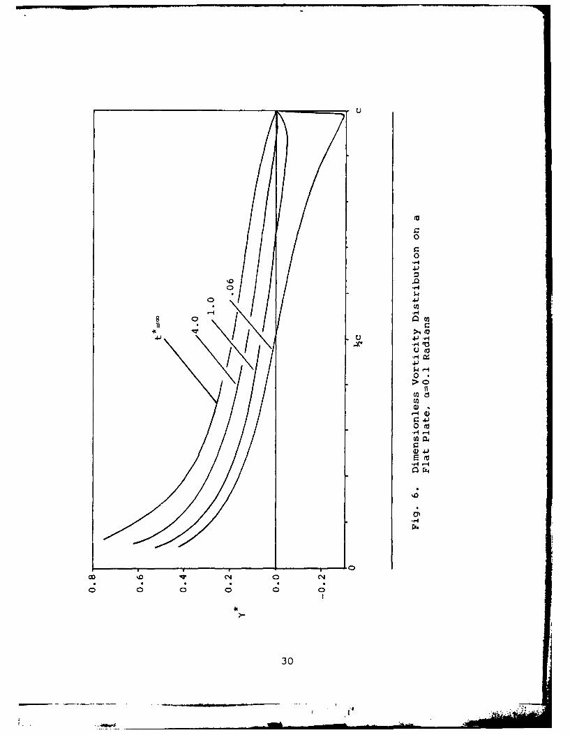
tendency with his numerical solution. Figure 6 depicts the

formation of the vorticity distribution y on a flat plate

at a = 0.1 radians, At 0.02 . Note that immediately

after the airfoil begins its motion, the vorticity is nega-

tive near the trailing edge, but as time passes, the vortic-

ity distribution approaches that for the steady-state condi-

tion. Shung (6:44) showed the same effect in his study

using a = 0.1 radians, At = 0.1 . In fact, his results

are identical to the results presented in Fig. 6. Similarly,

the build-up to the steady-state pressure difference distribu-

tion for a flat plate at a = 0.1 radians can be seen in

Fig. 7. Shung also demonstrated wake vortex sheet roll-up

behind an impulsively-started flat plate. The method of

28

-amp-4

I CN

0

41 Ln

0

-4

-k

4

041.a)

I ~4-I'4r-0

CNI

292

C.0

0

4.))

or

o 4-)

II-

0.(

-4

-4i -4

a 44

C20

300

-2.0-

AC -1. 0

006

0 'c c

Fig. 7. Pressure Difference Distribution ona Flat Plate, ct=0.l Radians

31

this thesis demonstrates the same phenomenon, as can be

seen in Fig. 8, which depicts wake vortex sheet roll-up for

the case of an impulsively-started flat plate at a = 0.1

radians, &t = 0.1 , the same conditions depicted by

Shung (6:43). Shung's depiction and Fig. 8 are almost iden-

tical.

The flat plate is, in fact, a special case of the more

general Joukowski airfoil, and other airfoils in this family

have been studied. Giesing (12) also developed a numerical

procedure to account for wake effects on the build-up of

lift on an arbitrary airfoil. Giesing published a curve of

C /C£ for a 25.5% thick symmetric Joukowski airfoil impul-ss

sively started at a = 0.01 radians. Using the same airfoil

and motion conditions, a CI/C curve was developed usingss

the numerical method presented in this thesis. Figure 9

compares those two curves with Wagner's curve for a flat

plate. As can be seen in Fig. 4, Giesing's curve predicts

values below those predicted by the present method. Whereas

the present method over-predicted C 2 for a flat plate, and

Giesing's method under-predicted C£ for a flat plate, it seems

likely that the ideal solution is bracketed by the present

method and Giesing's method. Both curves for the 25.5%

thick symmetric Joukowski airfoil show a greater delay in

lift production than does the flat-plate-airfoil curve. This

agrees with an analysis done by Chow, who showed that air-

foils of increased thickness develop lift at a slower rate

than thinner airfoils (13:14).

32:1 _ ____ ____ ___ ____ ____ __ - -

.9,1

0 041

0x

,-4

1 0

II ,-4

w

41

to

x

0 41

w

.s0 '0 0

0

33

IJA

-II :-.. ' ': _ . .. ..... ,., .-9"

4J-

0

0) 00 * 0

H e

U2 ) u0

0 0 3 -~ L4

CN/

o U'C

fo

0

u

0

C)-

al Cb0

344.

Giesing's numerical technique and the one presented in

this thesis differ in several ways. One major difference

between the two numerical techniques is in the way the motion

of the discrete vortices in the airfoil wake is predicted.

In Giesing's technique, after each time step, the non-dimen-

sional velocity induced at each trailing vortex position,

U , is calculated and then multiplied by At to approximately

predict where that discrete vortex will be at the next time

step. The non-dimensional velocity induced at that pre-

dicted position, Uc , is then calculated. The average of

U, + Uc is then multiplied by At to ccrrect the predic-

ted position of each discrete vortex for the next time step.

This method can be referred to as a Predictor-Corrector

method. The numerical technique presented in this thesis pre-

dicts the discrete vortex position in the same manner as

Giesing's predictor, but no corrector velocity is computed

or used. The predicted velocity is the only velocity used

to update vortex position.

To determine the effect a Predictor-Corrector method

has on the numerical solution, a program incorporating

Giesing's Predictor-Corrector method was developed. The re-

sults obtained using this program were compared with the re-

sults obtained using the method presented in this thesis

for the same airfoil and conditions of motion. Figure 10

shows a comparison of wake shape as computed by the two

methods for an impulsively started flat plate airfoil at

= 10 . Only in the area of starting vortex roll-up

35

t i, -" -- " .. I I IJl - ...

.. .Lwa

*Ai

--

00

0

94

II

W

x

4.1

00 • 0

00>

Q)

3 0.4I

, -" ,- ,• :IW ... .. ., •, 4i

does the difference in vortex position become apparent.

Further, the values of C /C computed using the two methodsss

are nearly identical, as seen in Table I. A comparison be-

tween the two methods was also made for the case of the flat

plate initially at a = 00 subjected to an e =0.035

One can see in Table II that the values of CX/CXs s computed

using the two methods are once again nearly identical. It

was thus determined that the added computation time incurred

by using the Predictor-Corrector method was not needed, and

thus not included in other studies in this thesis.

As a final check of the method of this thesis, the de-

velopment of y and aC on an impulsively-started symmetricp

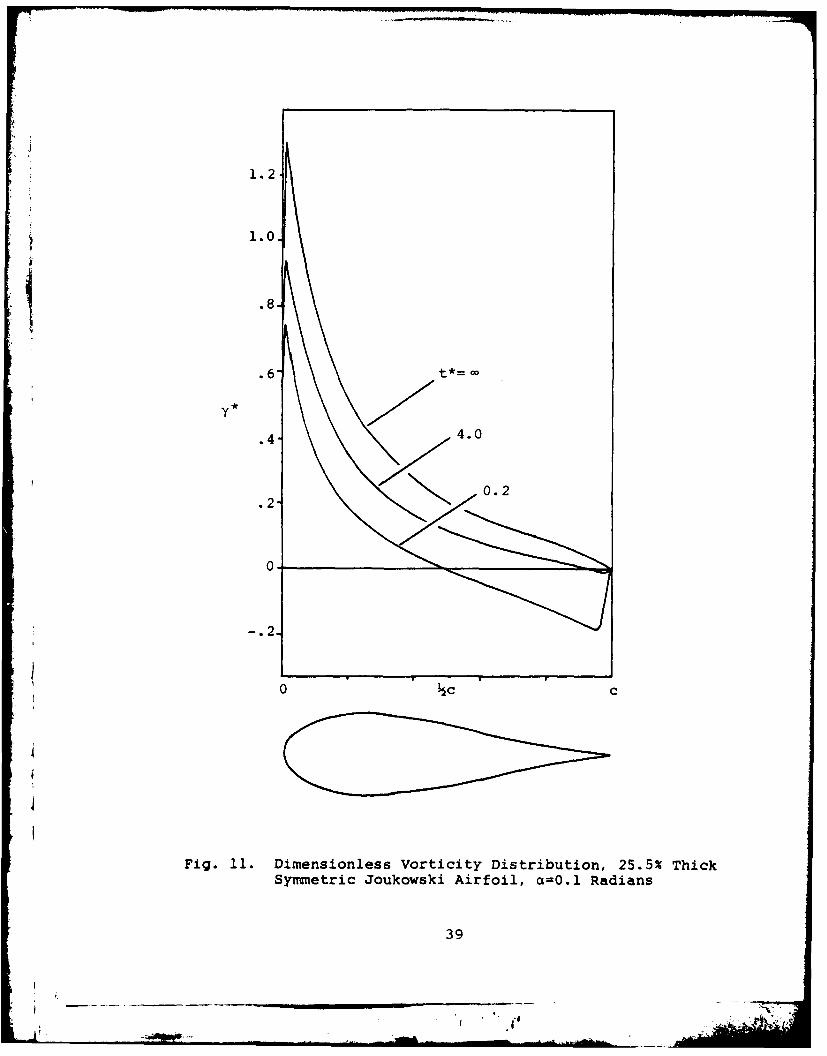
airfoil with thickness was determined. Figures 11 and 12

show that for a 25.5% thick symmetric Joukowski airfoil im-

pulsively started at a = 0.1 radians, y and LC build to

their steady-state values in much the same manner as for a

flat plate, Figs. 6 and 7, when using the numerical method

of this thesis.

It has been shown that for the test cases above, the

numerical method presented here is in good agreement with

the work of others (6;11;12;13). There are two major advan-

tages in using this numerical method over other methods.

First, unlike Shung, one is not limited to a flat plate.

Second, comparing to Giesing, the simpler method of vortex

motion prediction greatly decreases computer run time while

having a negligible effect on the prediction of lift build-

up on an airfoil.

37

Vow& , °,

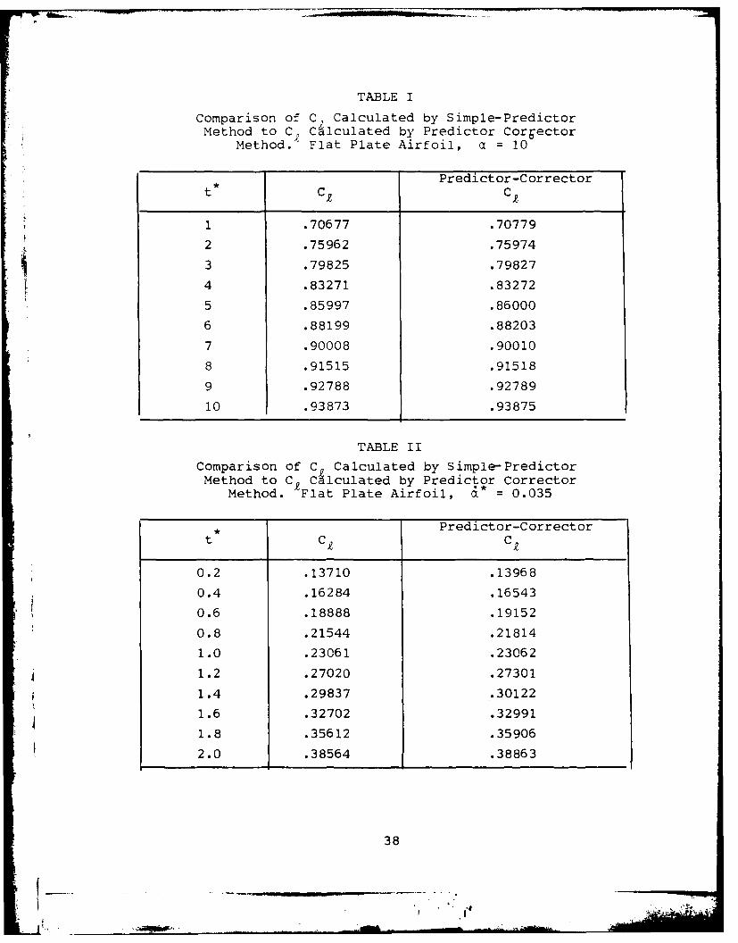
TABLE I

Comparison of C, Calculated by Simple-PredictorMethod to C Calculated by Predictor Corrector

Method.4 Flat Plate Airfoil, a = 10

Predictor-Correctort C2 C

2 1

1 .70677 .70779

2 .75962 .75974

3 .79825 .79827

4 .83271 .83272

5 .85997 .86000

6 .88199 .88203

7 .90008 .90010

8 .91515 .91518

9 .92788 .92789

10 .93873 .93875

TABLE II

Comparison of C Calculated by Simple-PredictorMethod to C2 Calculated by Predictor CorrectorMethod. Flat Plate Airfoil, a = 0.035

t *Predictor-Corrector

t C C

0.2 .13710 .13968

0.4 .16284 .16543

0.6 .18888 .19152

0.8 .21544 .21814

1.0 .23061 .23062

1.2 .27020 .27301

1.4 .29837 .30122

1.6 .32702 .32991

1.8 .35612 .35906

2.0 .38564 .38863

38

-:, !1 .- , I - -

1.2-

1.0.

.6-* 0

.4- 4.0

.2 0.2

0 c c

Fig. 11. Dimensionless Vorticity Distribution, 25.5% ThickSymmetric Joukowski Airfoil, ai=0.1 Radians

39

-3.0-

-2.0-

AC~

4.0

0.2

0

0 c c

Fig. 12. Pressure Difference Distribution, 25.5% ThickSymmetric Joukowski Airfoil, ca=0.1 Radians

40

Application to Constant-i Flow

In the last section it was shown that the present method

compares favorably to the results of others for the con-

stant-a, impulsively-started airfoil. In this section the

results of applying the method to the previously-unstudied

problem of constant- flow is presented. The presentation

of these results is broken into four parts in order to more

systematically explore and understand the interplay of pos-

sible effects. These four parts deal with the effects and

selection of starting conditions, the general effect of

on the build-up of C, the effect of thickness, and the ef-

fect of camber, respectively.

Selection of Standard Starting Conditions. As was

shown in the previous section, it takes some finite time for

an airfoil at angle of attack, a, suddenly placed into motion

to build to a steady-state value of lift. It is not sur-

prising, then, to find that the onset of constant a demon-

strates a different result depending on the time delay from

onset of impulsive motion to onset of constant a. The dif-

ferences, however, were found to be predictable, and thus

separable, as the following will show.

To determine the effect the initial a and a start time

have on the C vs. a curve for an airfoil at constant a, aiI

15% thick symmetric Joukowski airfoil with a = 0.01 ,

t = 0.02 was started at various initial a's and allowed

to build lift at that a for varying lengths of time t . For0 *

initial a = 0 , one can see from Fig. 13 that the time t

41

I ,,

.07.

It.06

.05

C .04' -

.03.

Steady State(-

.02 t = 0.2

= 1.0 (-o--.a.-).01Ja

0.1 0.2 0.3 0.4 0.50

ia

Fig. 13. Effect of Start Time to Begin a15% Joukowski Airfoil, ao=0?a*--0.01

40

42

.... . . .. - - -I: .

at which the . begins has no effect on the C vs. a curve.

For initial a = 5 , the C vs. a curves were dependent

upon the value of t at which the a was begun. However,

as can be seen in Fig. 14, the slope of the C vs. a

curve for a 0.01 does not depend upon the value of t

at which the a was begun. Choosing At = 0.1 , the 15%

thick symmetric Joukowski airfoil was allowed to build lift

to within 90% of steady-state C at various initial a's

before starting an a = 0.01 . As seen in Fig. 15, the

slope of the C vs. a curves for initial a's of 20, 4 and

60 are all approximately equal. The dashed lines on Fig. 15

depict the C vs. a curves that would be obtained by starting

the constant -a motion at full steady-state lift values

rather than the 90% steady-state lift values depicted by

the solid lines. Note that the initial value of CY obtained

for each of the starting angles of attack of 2 , 4 and 6

is the same amount above the steady-state C2 curve, and is

therefore independent of initial angle of attack. This ini-

tial value of C, will be called the 'jump' condition. Thus,

by the foregoing analysis, C 2 vs. a curve slope effects due

to the vortex wake will be assumed independent of initial a

and t.

The choice of At also shows some effect on the C vs.

a curve and was investigated. To do this, a 15% thick sym-

metric Joukowski airfoil at a = 0.01 was run at At

values of 0.2, 0.1, 0.02 and 0.004. Figure 16 depicts a

comparison of C£ vs. a curves for these four values of At

43

I , .

0.7-

0.6

CZ0.5,

0.4.

ta = 0. 2 (%C~start = 53% (,----)

ta = 1. 0(%C~start = 58%)

0.3.*t-= 3. 0(%C start = 64%)(--a)

5.1 5.2 5.'3 51.4 5.5

a0

Fig. 14. Effect of Start Time to Begina

15% Joukowski Airfoil, a0=50, a*=0.01

44

1.0

.9 /

.8 "

.7.[7

.77

.6-C,

/ = 20 (-.---,o-)

0•0 4 {

a°= 4° (-o----)

.3 a0 = 60 (6-)

.2

2 3 4 5 6 7 8 9

a 0

Fig. 15. Effect of Initial Angle of Attack to Begin a(C9 at 90% Steady-State Value)

45

* ,a.

.15-

. 10.

CL

.05 At

0.2 KQ-Q.0.1 (.-)

0.02 (0-)

.5 1.00

a

Fig. 16. Effect of At on C~ vs.* a Curve Slope

15% Joukowski Airfoil, a0 =00, a =0.01

46

Note that the slope of the curves, C2 , reduces as Ata*

is reduced, but the reduction is negligible below At = 0.02.

As a result of the above analysis concerning initial a

and t at which a is begun, all constant-a computer runs0 o *

assumed an initial a = 00 and t = 0 for a start-up. A

standard At = 0.02 was chosen as a reasonable value based

upon the information presented in Fig. 5 for impulsive-start

motion and Fig.16 for constant-a motion. While a At less

than 0.02 would produce more accurate results, the increased

computer time required at the smaller At values was judged

excessive for the slight increase in accuracy that could be

obtained.

General Effect of a on C * To determine the effect

an a has on the production of lift on an airfoil, a 15%

thick symmetric Joukowski airfoil was chosen as a represen-

tative airfoil shape. Using the selected values of initial

a = 00 and At = 0.02 , the airfoil was subjected to

various values of a ranging from 0.005 to 0.035. Figure 17

depicts the C vs. a curves obtained for small angles of

attack. Comparing with the C£ vs. a curve for the steady-

state case, one can see that as the value of a is increased,

the slope of the C2 vs. a curve, C. , is reduced. As thea

motion progresses to larger values of a, the slopes of the

curves increase slightly (see Fig. 18).

Effect of Airfoil Thickness on a Effect. The general

effect a has on the production of lift on an airfoil has been

shown. This effect was shown for a specific airfoil only.

47

-- _ _ _ _ _ _ _ __ _ _ 4.* .

0.3

0.2a=0.035

0.02

0.1100

0.005

1.0 2.0

0at

Fig. 17. Effects of a on CVS. a

15% Joukowski Airfoil

48

0.8

0.6

C7

0.4 7. ,

Steady0.2

ci = 0.035 (.---)

ci = 0.02 ('--)

0i ci

O

Fig. 18. C vs. a Slope Change as a Increases

at Constant a

49

APO2

To determine how airfoil thickness may influence this effect,

several symmetric Joukowski airfoils of varying thickness

were subjected to the same a conditions. Once again, values* 0

of At = 0.02 , initial a = 0 were used. Symmetric

Joukowski airfoils of 7%, 15% and 25.5% thickness, as well

as a flat plate airfoil, were subjected to a = 0.02. A

C vs. a curve can be plotted for each of these airfoils.

Plotting the average slopes of these curves, C£ , versus air-

foil thickness ratio t/c (where t is the maximum airfoil

thickness), one can determine the effect of airfoil thickness

on the C vs. a curve slope reduction due to a. Figure 19

depicts C vs. t/c for a = 0.02 . One can see that a2a

has a greater effect on lift curve slope reduction for thin

airfoils than for thick airfoils. This effect is consistent

with results previously presented. Note that in Fig. 9,

where a = 0 , for any given value of UAt/ c, the slope

of the CI/C ss curve is slightly greater for the 25.5% thick

symmetric Joukowski airfoil than for the flat plate. Al-

though the value of C2 /C£ is less for the airfoil withss

thickness, the rate at which C£/C2 is increasing is greater.ss

This implies that, under similar a conditions, C will in-

crease at a faster rate for a thick airfoil than for a thin

airfoil. Figure 19 confirms that conclusion.

Effect of Airfoil Camber on a Effect. In much the same

way as airfoil thickness effects are calculated, airfoil

camber effects can also be explored. Joukowski airfoils of

15% thickness at various camber ratios were subjected to an

50

('40

44

I1I

44

u,.

_4

U

-

-4

0-.,

S4

L)2

51U

51I

= 0.02 As before, initial a was 0 , At = 0.02

Plotting average C versus camber ratio (maximum camber/

chord), camber effects can be shown. Figure 20 depicts C2

vs. camber ratio for 15% thick Joukowski airfoils of various

camber ratios. One can see that a has a greater effect on

lift curve slope reduction for less cambered airfoils than

for highly cambered airfoils.

52

4 N4

0

44E $4

rz

-H .

Li 44I

co %.0

532

IV. Conclusion

It has been shown that as an airfoil pitches at a con-

stant a, the airfoil trailing vortex wake causes the slope

of the C vs. a curve to be less than the slope of the CI vs. a

curve for steady-state a. The greater the value of a for a

given airfoil, the greater the slope reduction of the C. vs. a

curve caused by the vortex wake. This effect becomes less

pronounced as airfoil thickness increases. Similarly, the

effect is also less pronounced as airfoil camber increases.

Using the results from the previous section, the follow-

ing predictions of constant-a effect may be made.

For a flat plate, the reduction in C. may be approx-a

imately calculated by

C( .15 1 + 2 2 (49)

a( + 0.00008)0.15

(See Fig. 21 for a comparison of this prediction with numer-

ical data.) This prediction may be approximately corrected

for thickness by adding a correction term derived from Fig.

19. Thus

t 0.75Ca ,t/c) = ( ) + C(*) (50)aL a (0

where t/c is the airfoil thickness to chord ratio and

C£ (cI) is the C. vs. a curve slope for a flat plate pre-

dicted by Eq. (49). A further approximate correction may

be made for camber by adding another correction term, de-

rived from Fig. 20. Thus

54

4 -,,__ __ . I 1 I I

CN 4-4

+ 0

U, 0-- 4

ji,

o to-. 440

00

+ I

o n

5 ISI U"

II

.I1(

1 0• -4

55

C (a* t/cmc/c) e 3 0(mc/c-0.09) + C (a *,t/c) (51)

where mc/c is the airfoil camber ratio and C (a/) is

the C vs. a curve slope for an airfoil with thickness pre-

dicted by Eq. (50).

The amount that CI increases immediately after an air-

foil begins constant-a motion is referred to as the 'jump'

condition. This value for a flat plate can be predicted by

AC(a) = 3.47a* (52)

where AC (a) is the 'jump' condition change. Thickness

effects on AC (a ) can be approximated by the equation

AC (a*,t/c) = [l + 2(t/c)]Ac2 (d*) (53)3

where t/c is the airfoil thickness ratio and AC2 (a ) is the

'jump' condition for a flat plate defined by Eq. (52). A

final approximate correction to the 'jump' condition can be

made by

AC( t/c, mc/c) AC(a, t/c) - 1.3(-mc) (54)

where mc/c is the airfoil camber ratio and AC2 (cL, t/c) is

as defined by Eq. (53).

56

'

V. Recommendation

The assumption that the trailing vortex wake of an air-

foil undergoing a constant rate of change of angle of attack

has a negligible effect on the production of lift on the air-

foil is not, in general, valid. Although the effect is not

jlarge (see Eq. (49)), it should be accounted for in the in-

vestigation of dynamic stall of airfoils. The methods de-

veloped by Docken (4) and Lawrence (5) could be modified to

include the techniques presented in this thesis to more ac-

curately predict the potential flow field about a pitching

airfoil at any instant in time. Incorporating the calcula-

tion of wake vortex effects outlined in this thesis into

Lawrence's work would significantly contribute to the solu-

tion of the dynamic stall problem for an airfoil undergoing

a constant rate of change of angle of attack.

57

I,

APPEND I X: Computer Prog ram

CC This program computes circulation, pressure differenceC distribution, vorticity distribution, coefficient ofC lift, and trailing vortex wake shape for a 2-D JouKowsKiC airfoil in an incompressible, inviscid free stream atC tangle of attack. The angle of attack may be a constantC value, or it may be changed at a constant rate for theC number of time steps desired. All output values areC computed ,assuming a trailing vortex wake made up of dis-C crete point vortices of constant strength, each of whichC influences the motion of all the other vortices and theC flow about the airfoil. For the constant rate-of-chanae"I of ingle-of-attack case, coefficient of lift can beC ;ound ,as a function of the rate of change of angle ofC attack. Variables in the program are defined as follows:C

C alf a - angle of attackC iallf-2 - initial angle of attackC alfdot - time rate of change of angle of attackC beta - the beta parameter of a JouKowsKi airfoilC cal fa - COSINE of alfaC chord - airfoil chord length

cl - coefficient of liftC ciss - steady-state coefficient of liftC countt - 'an integer counter used to determine whichC time steps will record output in certainC fiesC ct.heta - COSINE of theta1C d'a.. fa - increrental change of alfaC ~oeizo - array of incremental values of coefficientC of pressure along the airfoil chordC deld - distance on the x-axis in the cylinderC plane behind the cylinder where the firstC shed vortex is placedC delgam - array of values of strengths of gamma forC each individual vortex pairC dgoams - a sum of vortex strengthsC dsl - incremental distance along airfoil lowerC surfaceC dsu - incremental distance along airfoil upperC surfaceC dt - incremental unit of timeC Z - complex number; derivative of theC JoukowsKi transformajtionC dz&-c - rn,,agnitude of c ZD

'S e..t,.a - x .' u~e of trailing vortex position

58

-W 0

C eta2 - x-value of trailing vortex image positiong a mmnI - airfoil circulation

C i,.jK,1 - integer values used in iterationsC intgrl - value of the integration of velocityC differences between upper and lowerC airfoil surfacesC lastdt - last time increment at which alfa changesC mag2 - distance from a vortex to the center of theC cylinder in the cylinder-centered planeC malfa - maximum value of alfaC maxdt - first time increment at which alfa changesC from alfaOC max.t - last time stepC MU - complex number; distance between the originC in the displaced-cylinder plane and the

C center of the cylinderC pi - the constant 3.14159265C RHO - complex. r number; a position in the cylinder-C centered planeC RHOP - complex number; a position in the displaced-C cylinder planeC sl.fa -.SINE of alfaC ssgam - steady state value of circulationC stheta - SINE of thetaC sumsqr - the square of the distance of a trailingC vortex from the origin in the cylinder planeC sumu,suMv - sum of the velocities on the cylinder inC the x and y directions, respectively, in-C duced by trailing vortices and their imagesC t - integer counter for number of time stepsC theta - angle measured counterclockwise from theC '.-axis in the cylinder planeC totutotv - sum of velocities ,at 'a vortex location *.nC the x and y directions, respectively, in-r - duced by trailing vortices and their imagesC UIv - velocities at a vorte.' location in theC x and y directions, respectivelyC ua,va - velocities at a vortex location in theC x and y directions, respectively, in theC airfoil planeC usurf,vsurf - velocities on the cylinder in the x and yC directions, respectivelyC utheta - velocity tangent to the cylinderC vordis - vorticityC vsqare - velocity on upper surface of airfoilC squared minus velocity on lower surfaceC of airfoil squaredC x'y - position on airfoilC .,vort.yvort - position of a trailing vortex

Z- compl.ex number' a position on the airfoilC zet: .- y v'lue of trailing vorte. positionC :qt,.2 - y v' ,-e of trailing vortex image position

59

1 (t'mmL. ".. .. -] . , k. i )- -l rf :-

C zt - distance 'alona x-axis fror, origin toC cylinder in displaced-cylinder plone

C Z - complex number; 'a position in -the waKe inC the airfoil planeCC FILES:*

-~ C

C INPUT - unformatted list of input variablesC OUTPUT - list of C1 vs. C1 steady-state for angle ofC attack and time stepC PRES' - pressure distribution at specified time

C VORT - vorticity distribution at specified time.C WAKE - position of trailing vortices at specified time

IMPENSION zeta(201,201),et'a(201,201),eta2(201,201),

+zet'-18:1(0,20-1,(01,0)vht(20101,delg (201),.0)

+v"2(201 ,201) ,xvort(201 ,201) ,yvort(201 ,201),rvordis(0: 176) ,delcp(0: 176) ,intgrl(0*201,0U*80)INTEGER i,.j,m'axt,tpK,lvrnaxdtycounttREALh delgam,deld,pi ,cthetarsthetarssgampdsurdslrdelcp,+ujsurf~vs'irfptheta,utheta,gamia,malfa,alfarsumu,sumv,+dalf'a rdgars calf a, salfa, sumsq r, alf dot, dt, dzd ro, ua Pva,+beta,zt,ailf'aO,clsscl,,ytvsqare,x,,vortryvort,lastdt,+et':-,2.zeta:.---eta2, uvvchord,intgrl,totui,totvpvordis,+ na g 2, et'a

COMPLEX MU,RH0P,Z,ZZ,RHODZrOPEN (15P.FILE="'INPUT')REWIND 15fJF'EN (16,FILE=CUTFUT')REWIND 16PEN "'17 .FILE="PRESD')

OPEN (18,FILE='WAKE')REWIND 18OPEN (1?,P.tLE='VORr')REWIND 19

pi=3. 14159265

C Initialize delta alpha, delta d, max to Compute steadyC state gamma,

10 CONTINUE

REAI( 15?*,END=400) beta,alfa0,dalfa,deld ,maxdt,maxt,+lastdt,zt,alfdot,dtmalfia=dal1fa*( lastdt-rn'axdt)+'alftaO0ssgcm=~4*pi*SIN ( malf'a*p i/!G0)WRITE(16,70) zt1.beta,dalf'a,dclid, ssg:iv alFdct it

4WFRTTE( 17Y72) zt,bet,a'aj~lf'a~deJIdrsscaairir,'fdot ,dt

60

WRITE( 18,72) zt,betard'af', deid ,SCrg'IrIT,afdot,dtWRTTE(19,72) ztpbetavd'aliardeld,ssgaiT~,afdotrdtbet a be tia* p i/180d al1fia =dal a *p i/i80QifQO=alfia*p i/iSOMU=CMPLX(zt-COS(beta),SIN(beta))

CC Cialculiate coordinates of points on the airfoil* (x,y)I C DO 15 i=-180,180

thetea=i*pi/180RHOP=CMPLX(COS(theta-beta) ,SIN(theta-beta) )+MUZ=RHOP+t**2/RHO'x( i )REAL(Zy( i)=AIMAG(Z)

15 CONTINUEchnord.x (0)-x-80+2*b eta)DiO 12 i=1,mtaxtA

delgari( i )0.0'2 CONTINUE

DiO 13 i=176,0r-4intgrl (0, i =0,

13 CONTINUECC Begin stepping in time, inserting 'a new vortex pair 'atC e'ach time step.C

cowl tt=0riO 300 t=1,maxt

count t = co uftt +intgri (t, 18O)0,.

dcam0 0.

IF (t.GErrgaxdt,'ard .t.LE. iastdt) THEN

ELSE IF(1,.LT.mo'xdt) THEN'a if 'a='af 'a0

END IFc'aifa=COS(alfia)s a if'a =SIN (a if'a)

CC Insert new vortex pair, and update position of ail other

4C vortex imaiges.

C zet'a(t,1)=deld+1#

et'act, )=0.xvort (t, 1)=chord*dt*COS (2*beta) /2+x (0)yvort(t,1>=chord*dt*SIN(2*beta)/(-2)

rDO 20 j=",t

61

Calculiate strength of newly shed vortex at timge t.CThis is done by siatisfying the Kutta Condition a~t the

tr'ailing edge while Keeping totoal circulation in theC field equal1 to zero.C

delgam(l)=4*Kpi*salfa*(zeta(tpl)**2+etc(t,1)**2+1-2*

IF(t.GE.2) THEN

1+ /1 (zeti(t, 1 *+et(t, 1 *2-1) cyl~tile

21 CNTIUEdelgan(1)/(4*pi*salfa)

0 -at time t0

D00 30 =t1,-P17

+ zetma=tCk) **2+the'-taa,))*)+sht+ heta=S(the)/(the -e)(~))*+sht~+ uu= e .0~K>*))sm

sumu'=d e g'ns(K )/2/p i (eteoe(t rK)kst))/(c theta-+ zta(t,K))**2+(sthet'1-etQ(trK) )**2)-(s(thets-+ eta2(t,K))/((ctheta-eta2(t,K))**2+(stheta-+ eta2(t,K))**2'))+sunmv

30 CONTINUEusurf=2 *(calf'a*sthetga**2-cthet*sthet*salfa)+sumuvsurf2*(slf*cthta**2-ctheta*stheta*c.1lfa)+sumvuthe'a ( i )=SGRT (usurf'**2+vsiirf**2)IF(i.NE*0) THENRHOP=CMPLX(COS(thet-beta) SIN(theta-beta) )+MUDZD1 -zt**2/RHOP**2dzd roinAIS (DZD)jutheta( i)=utheta~i )/dzdro

END IFIF((theta-(olfa+2*betGi)).LT.-1*pi) THEN

uthet'2(i)=-1*utheta(i)END IF

200 'CONTINUEgQMMrn3=0.DO 210 i=1,t

g a rr 7 i -3 d elcrqnQ m

62

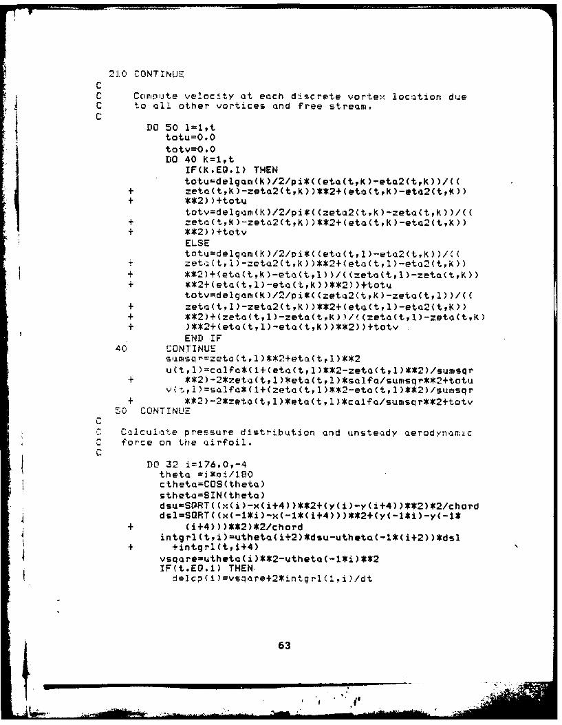
210 CONTINUECC Compute velocity at each discrete vortex location dueC -to all other vortices and free stream.C

ElO 50 1=1,t

DO 40 lpIF(K.EO~l) THEN

+ zeta(tk)-zeta2(tk) )**2+(eto(tk)-eta2(tk))+ **2))+totu

totv=delg'am(R )/2/pi*( (zetaa2(tpK >-zet:(t,K) )/((+ zeta(tpK )-zet'a2(tK) )**2+(et'a(tk )-eta2(tpK))+ **2))+totv

ELSEtotu=delgar(K )/2/pi*( (et'a(t,l1)-etra2(t,K) )/((

+ et.a(ti)-zetia2(tpK> )**2+(et'a(t,l)-et'a2(tK))+ **2)+(etea(tK)-eta(t,l) )/( (zeta(t,l)-zeta(tK))+ **2+(et'a(t,1)-et'a(t,K) )**2) )+totu

totv=delgar(K)/2/pi*((zeta2(t,K)-zeti(t,l))/((+ zet'a(t,l)-zet'22(t,K))**2+(eta2(t,1)-etc2(tK))+ **2)+(zetcl(t,l)-zeta(tK) )/( (zeta(t,1)-zetG(t,K)+ )**2+(et'a(t,1>-etaa(t,K) )**2) )+totv

END IF40 CONTINUE

su-nisqrzeta(tpl)**2+eta(t,1)**2u(t,1)=calf'a*(1+(eta(t,1)**2-zeta(t,l)**2)/sumsqr

+ **2)-2*zeta3(t,l)*eta(t,l)*salfa/surnsqr**2+totuv( , )=salf'a*( 1+(zeta(t,l1)**2-et'a(t,l1)**2)/suimsqr

+ **2)-2*zeto(t,1)*eta(t,l)*calfo/sunsqr**c2+totv50 CONTINUE

CC Calcu'a te pressure dist-ibution 'and unsteady 'aerodynam.c

0 force on the 'airfoil.C

DO 32 i=176,0,-4theta =i*oi/18Octheta=COS(theta)sthetaSIN(theta)dsu=S0RT((x(i)-x(i+4))**2+(y(i)-y(i+4))**2)*2/chorddsl=SQRT( (x(-l*i)-x(-1*(i+4)))**2+(Y(-l*j)-Y(-1*

+ (i+4)))**2)*2/chord

+ +intgrl(tpi+4)vsq'areutheta( i )**2-utheta(-l*i )**2IF(ti.EG.1) THEN.

63

how", jd- K

ELSE IF(t.EQ.2) THENdel cprjC) =vsqare+2*(intgrl(2,i)-initgrl(1,i) )/dt

E'LSE IF(t.Eq.iaxdt) THENdelcp Ci )vsqare+2*intgrl (rYiaxdt i )/dt

ELSE IF(t#E.mia>:dt+1) THENdelcp(i )=vsqcire+2*(intgrl (rnoxdt+1 , i)-

intgrl(m'axdt, i) )/dt* ELSE

delcp.(i )=vsqare+(intgrl (t-2,i)+3*intgrl(tpi)-4*+ intgrl(t-Ii))/dt

END IFIF(i*EQ*176) THENclcl+delcp(176)*(x(174)-x(180) )/chord

ELSE IF(i*EO.0) THENclcl+delcp(0)*(x.(0)-x.(2))/chord

ELSEcl=cl+delcp(i)*(x,(i-2)-x-(i+2))/chord

END IFA CTNTINUE

CC Calculate Cl.C

c is s =8 *pij/ crd * s a 1 iIF(t%.EO,3) THEN

+ t,t*dtWRITE(1S','('Vorticity Distribution 5,13.

+ ' Vortices, t=',F7.4)') t,t*dtDO 34 i=176,0,-4vordis(i)uitheta( i)-utheti(-l*i)WRITE C19,90) (t( i )+chord-2*zt)*2/chord ,vordisC i)WRITEC17,90) (,, i )+chord -2*zt) *2/cho rdv-1*delcp (i)

34 CONTINUIEEND IFI'F(counrtt/I.C.G T.*0) THEN

WRITE(17,'('Deltai Cp,.',13, U Vortices, t=',F7.4)')+ trt*cit

WRITE(19,/C'Vorticjty Distribution 5,137

+ '3 Vortices, t=,F7.4)') t,t*dt

WRITE(19,90) (x(i )+chord-2*zt)*2/chordpvordis( i)4 WRITE(17P90) (x(i)+chord-2*zt.)*2/chord,-l*delcp(i)

35 CONTINUEC ou.fltt=O

END IF

+ *2/chord,yvort(tpt)*2/chord,gmmac,clss,clC

C Move e'achi vortex t~o its new location in the flow field.

64

D[1 60 KRt,l,-1mac2=SRT(zetc1(t1 K)**2+et'3(t,k )**2)RHO,:P'=i,ra2*MFLX(CS(COS(zeto(t,K )/mag2)-bet a),

+SIN AS IN (eta( t,K )/Ym'ag2)-beta) )+MUD ZD'=1- zt * *2/R H OF** 2dzdro=ABS(DZD)

v'a(tK )=v(t,K )/dzdroxvort(t+lK+1)=xvort(tIO+ua(t,.O)Kchord*dt/2yvort(t+lK+1)=yvort(tK)+va(t,K)*chord*dt/2ZZ=CMPLX(x<vort(t+lPK+1),yvort(t+1,K+l))RHD=( (ZZ+ SORT(ZZ'K*2-4*zt**2) )/2-MU)*

+ CMPLX(POS(bet'a),SIN(beta))zetQ(t+1 ,K+1 >REAL(RHO)etga(t+1 ,K+1 )AIMAG(RHO)clelgamr(K+1 )=delgorn(K)

*60 CONTINUEI!F(t.EO.5) THEN

GO TO 61ELSE IF (t.EQ.mox-dt) THEN

00 TO 61ELSE IF(t.EQ.lastdt) THEN

GO TO 61ELSE IF(t.EG.maxt) THEN

0O TO 61ELSE

GO TO 300END IF

61 WRITE18,1'Wa~e Vortex Locations from Trailing',+' Edge (1/2 c = 1)'/" Xvort',5X,'Yvrt')')

DO 65 i=l,t* WRITE(18,95) (xvort(t,i)-x(Ofl*2/chordv

65 & CONTTNUE ± r1,(v)*2/chord

00 CONTINUE70 FGRMAT(///,'AIRFOIL DATA :',//,'Zeta~ trailing edge '

+F7.4,' Beta (deorees):1F63,//,YNAMIC PARAMETERS',+//,'D~elta Alpha (degrees):',F6.3,' Delta Vortex+ rigt'nce:',F6.4,/,'Ste:idy State Gamma:' '7F7.57+' Alpha Dot:',FB*5,' Delta Time:',F5.3,//,'Tine',1OX,+'S0tarting Vortex',17X,'Cl',/,'Step Alpha X

+1 Y Gamma Steady State C11,/)72 FORMAT(///,'AIRFOIL DATA :'p//,'zeto trailing edge '

+F7.4,' B~eta (dwgrees)1,1F6.3r//,'DYNAMIC PARAMETERS',+//,'Delta Alpha (degre~s)**',F6.3,' Delta Vortex '+'Distance*',F6.4,/,'SteadY State Gamma: 1,F7*5,+' Alpha Eot:',FS.5,' Delta Time#0',F5.3,/)

80 FORMAT(13, 3XF6.3, 2X,F7.4,FB.4,1X,FS.5,SX,FB.5,2X,F8.5)90 FORMAT (FS .3,4X,F1O .5)?5 FCRMAT(FS.4 , F1l 4)

65

Bibliography

1. Kramer, von M. "Die Zunahme des Maximalauftriebes vonTragflugeln bei plotzlicher AnstellwinkelvergroBerung(Boeneffekt)," Zeitschrift fur Flugtechnik und Motor-luftschiffahrt, 7: 185-189 (April 1932).

2. Deekens, A.C. and W.R. Kuebler, Jr. "A Smoke TunnelInvestigation of Dynamic Separation," Aeronautics Digest,Fall 1978. USAFA-TR-79-1, Air Force Academy, CO.Feb 1979.

3. Daley, D.C. The Experimental Investigation of Dynamic

Stall. Thesis, AFIT/GAE/AA/82D-6. Air Force Instituteof Technology, Wright-Patterson AFB, OH, 1983.

4. Docken, R.G., Jr. Gust Response Prediction of an Air-foil using a Modified vonKarman-Pohlhausen Technique.Thesis, AFIT/GAE/AA/82D-9, Air Force Institute ofTechnology, Wright-Patterson AFB, OH, 1982.

5. Lawrence, Maj J.S. Investigation of Effects Contributingto Dynamic Stall Usa a Momentum-Integral Method.Thesis, AFIT/GAE/AA/83D-12. Air Force Institute ofTechnology, Wright-Patterson AFB, OH, 1983.

6. Shung, Yeou-Kuang. Numerical Solution for Some ProblemsConcerning Unsteady Motion of Airfoils. Ph.D. disserta-tion. University of Colorado, Boulder, CO, 1977.

7. Spiegel, Murray R. Theory and Problems of Complex Vari-ables. New York: Schaum's Outline Series, McGraw-HillBook Company, 1964.

8. Kuethe, Arnold M. and Chuen-Yen Chow. Foundations ofAerodynamics: Bases of Aerodynamic Design (Third Edition).New Yorks John Wiley and Sons, Inc., 1976.

9. Milne-Thomson, L.M. Theoretical Aerodynamics (ThirdEdition). London: Maaillan and Company Limited, 1958.

10. Karamcheti, Krishnamurty. Principles of Ideal-FluidAerodynamics. New Yorks John Wiley and Sons, Inc., 1966.

11. Von Wagner, H. "Dynamischer Auftrieb von Tragflugeln,"

Zeitschrift fuer Angewandte Mathematik und Mechanik, 5:17 (February 1925).

12. Giesing, Joseph P. "Nonlinear Two-Dimensional UnsteadyPotential Flow with Lift," Journal of Aircraft, :135(March-April 1968).

4... 66 .6

13. Chow, Chuen-Yen and Ming-Ke Huang. "The Initial Liftand Drag of an Impulsively Started Airfoil of FiniteThickness," Journal of Fluid Mechanics, 118:393-409(May 1982).

V

67/

- *1

VITA

Captain Kenneth W. Tupper was born on 22 April 1952 in

Johnson City, New York. He graduated from high school in

Meadville, Pennsylvania, in 1970 and attended the United

States Air Force Academy from which he received the degree

of Bachelor of Science in Astronautical Engineering in June

1974. Upon graduation, he was commissioned a Second Lieuten-ant in the USAF. He completed pilot training and received

his wings in July 1975. He served as a KC-135 pilot and

flight instructor in the 924th Aerial Refueling Squadron,

Castle AFB, California, until entering the School of Engi-

neering, Air Force Institute of Technology, in June 1982.

Permanent address: 978 Northwood DriveMerced, California 95340

68I , , - A- - s--

UNCLASSIFIEDSECURITY CLASSIFICATION OF THIS PAGE A-6-s (A~ 2

REPORT DOCUMENTATION PAGE1& REPORT SECURITY CLASSIFICATION lb. RESTRICTIVE MARKINGS

UNCLASSIFIED2a. SECURITY CLASSIFICATION AUTHORITY 3. DISTRIBUTION/AVAILABILITY OF REPORT_Approved for public release;

21. DECLASSIFICATION/OOWNGRAOING SCHEDULE distribution unlimited.

4. PERFORMING ORGANIZATION REPORT NUMBER(S) S. MONITORING ORGANIZATION REPORT NUMBER(S)

AFIT/GAE/AA/83D-24

Ga NAME OF PERFORMING ORGANIZATION b. OPFICE SYMBOL 7. NAME OF MONITORING ORGANIZATION(if fapilbia)

School of Engineering AFIT/EN6c. ADDRESS (City. State and ZIP Code) 7b. ADDRESSI (City. State and ZIP Code)

Air Force Institute of TechnologyWright-Patterson AFB, Ohio 45433

ft NAME OF FUNOING/SPONSORING 9S1. OFFICE SYMBOL 9. PROCUREMENT INSTRUMENT IDENTIFICATION NUMBERORGANIZATION (If applica b )

Se. ADDRESS (City. Stat. and ZIP Code) 10. SOURCE OF FUNDING NOS.

PROGRAM PROJECT TASK WORK UNITELEMENT NO. NO. NO. NO.

11. TITLE (include Security Cluamuflation)

See Box 1912. PERSONAL AUTHORIS)

Kenneth W. Tupper, B.S., Capt, USAF13& TYPE OF REPORT 13b, TIME COVERED 114. OATS OF REPORT (Yr.. Mo Day) 11S. PAGE COUNT

MS Thesis FROM ___ TO___ 1983 December 80. SUP'PLEMENTARY NOTATION A..yj.. .reeo: AW AFa 1g . JAN d4

De Ln-orI ;eachc.. ond Pre|ioF i avl ,

17. COSATI COOS 1 SUBJECT TERMS (con r "Aw.y b numbr)PIELO GROP SUS. OR. Wake Vortex E*90,4fot tall, Potential20 04 Flow Vortex Wake, Starting Vortex

1S. ABSTRACT lContinue on a d if syearn, and identfy by block numbar)

Title: THE EFFECT OF TRAILING VORTICES ON THE PRODUCTIONOF LIFT ON AN AIRFOIL UNDERGOING A CONSTANTRATE OF CHANGE OF ANGLE OF ATTACK

Thesis Advisor: Eric J. Jumper, Major, USAF

20. OISTRI.UTION/AVAILAILITY OF ABSTRACT 21. ASTRACT SECURITY CLASSIFICATION

UNCLASSIPIME/UNLIMITED 3 SAME AS rPT. " OTIC USERS 0 UNCLASSIFIED

22& NAME OP RISPONSIBLE INDIVIDUAL 22b. TELEPHONE NUMBER 22C. OFFICE SYMBOL(include Area Coda)

IEric J. Jumper, Major, USAF 513-255-2998 AFIT/EN

00 FORM 1473.83 APR EDITION OF I JAN i IS OBSOLETE. UNCLASSIFIEDSECURITY CLAESIPICATION OP THIS PAGE

UNCLASSIFIED

SECURITY CLASSIFICATION OF THIS PAGE

This study explored the effect of a trailing vortexwake on the production of lift on an airfoil.undergoing aconstant rate of change of angle of attack, a. Thq studyshowed that when an airfoil encounters a constant-a flow,the trailing vortex wake acts to suppress the slope of theairfoil's C, vs. a curve. The change in magnitude of thiseffect as a function of airfoil thickness and camber wasalso investigated.

Potential flow theory was used to model the flow abouta two-dimensional circular cylinder, and that flow was trans-formed to flow about an airfoil by the Joukowski transforma-tion. The trailing vortex wake was modeled by a sequence ofdiscrete point vortices, and the pitching motion of the air-foil was modeled by a series of small incremental changesin angle of attack, Am, over a short period of time, At.The rate of change of angle of attack, i, was then definedas Am/At. After each time change At, a was changed by anamount a. A discrete vortex was introduced into the wake ata distance UAt behind the airfoil trailing edge, and abound vortex of equal strength but opposite sense was intro-duced to satisfy the Kutta condition and keep the total cir-culation in the flow field equal to zero. As each new vor-tex pair was introduced, all other trailing vortices wereassumed to move in the wake by a distance UAt, where U isthe velocity induced at a vortex position by all other trail-ing vortices, the bound vortices, and the free stream flow.The unsteady Bernoulli equation was solved using numericalintegration and differentiation techniques to determine pres-sure difference distribution, vorticity distribution, andcoefficient of lift on the airfoil for that instant in time.This information was then used to investigate the overalleffect of constant-6 flow a$ well as the effect of thicknessand camber on the constant-a problem, and simple rules forpredicting the effects were developed.

4

UNCLASSIFIEDSECURITY CLASSIFICATION OF T,1 PAGE

J ,