SECURI IFIC QN F T AIe

Form ApprovedREPORT DOCUMENTATION PAGE OMB No. 0704-0188

la. REPORT SECURITY CLASSIFICATION lb. RESTRICTIVE MARKINGS

UNCLASSIFIED NONE2a. SECURITY CLASSIFICATION AUTHORITY 3. ,

2b. DEC[ DIS IIBUTION UNLIMITED

4.A D- 217 955 S. MONITORING ORGANIZATION REPORT NUMBER(S)AFIT/CI/CIA-89-127

6a. NA K A I bo. u,.i,. SYMBOL 7a. NAME OF MONITORING ORCANIZATIONT+ OSIV N (If applicable) A FIT/CIAOF OKLAHOMA1

6c. ADDRESS (City, State, and ZIP Code) T. ADDRESS (City, State, and ZIP Code)

Wright-Patterson AFB OH 45433-6583

8a. NAME OF FUNDING/SPONSORING 8b. OFFICE SYMBOL 9. PROCUREMENT INSTRUMENT IDENTIFICATION NUMBERORGANIZATION (if applicable)

Bc. ADDRESS (City, State, and ZIP Code) 10. SOURCE OF FUNDING NUMBERSPROGRAM PROJECT TASK WORK UNITELEMENT NO. NO. NO. ACCESSION NO.

11. TITLE (Include Security Classification) (UNCLASSIFIED) E I

A Comparison of Deterministic Lot Sizing Techniques Using Focum Forecasts of StochasticDemand Data

12. PERSONAL AUTHOR(S)

Bryan Stewart Cline13a. TYPE OF REPORT 13b. TIME COVERED 14. DATE OF REPORT (Year, Month, Day) 15. PAGE COUNT

THESIS FROM TO 1989 18616. SUPPLEMENTARY NOTATION APPROVED FOR PUBLIC RELEASE IAW AFR 190-1

ERNEST A. HAYGOOD, Ist Lt, USAFExecutive officer, Civ n tn P-rern-,

17. COSATI CODES 18. SUBJECT TERMS (Continue on reverse if necessary and identify by block number)FIELD GROUP SUB-GROUP

19. ABSTRACT (Continue on reverse if necessary and identify by block number)

OTIC -,

elt f-!.ECTE ,FEB 13 1990

20. DISTRIBUTION /AVAILABILITY OF ABSTRACT 21. ABSTRACT SECURITY CLASSIFICATIONnUNCLASSIFIED/UNLIMITED 0 SAME AS RPT. 0 DTIC USERS UNCLASSIFIED

22a. fA MlEf PESPQ.I UDIVI , DUAL 122b. TELEPHONE (Include Area Code) 122c. OFFICE SYMBOL1•tNI A... , Lst 't, S S 513-255-2259 AFIT/CI

DO Form 1473, JUN 86 Previous editions are obsolete. SECURITY CLASSIFICATION OF THIS PAGE,

THE UNIVERSITY OF OKLAHOMA

GRADUATE COLLEGE

A COMPARISON OF DETERMINISTIC LOT SIZING TECHNIQUES

USING FOCUS FORECASTS OF STOCHASTIC DEMAND DATA

A THESIS

SUBMITTED TO THE GRADUATE FACULTY

in partial fulfillment of the requirements for the

degree of

MASTER OF SCIENCE

By

BRYAN STEWART CLINE

Norman, Oklahoma

1989

* ( 1 -

A COMPARISON OF DETERMINISTIC LOT SIZING TECHNIQUES

USING FOCUS FORECASTS OF STOCHASTIC DEMAND DATA

A THESIS

APPROVED FOR THE SCHOOL OF INDUSTRIAL ENGINEERING

Acce';gon For

NTIS CR&

DTIC IAH UU ;:': ': ,d U.

..........-.-- By

By 2B

Dist L'n I".ceL5 1

Acknowledgements

I would like to thank my mentor, Dr. Foote, for the

time, effort, and patience he expended in my behalf.

Without his guidance, this research would not have been

possible.

I also offer my sincere appreciation to the other

members of my committee, Dr. Schlegel, Dr. Leemis, and Dr.

Pulat, who have helped me, not only in this endeaver, but

throughout my entire Master's program. Dr. Schlegel

deserves special recognition for taking over the

chairmanship of my committee when Dr. Foote was unable to

attend my defense.

I also owe Capt. G. Mark Waltensperger a note of thanks

for the many long hours we spent working together. His

moral support was integral to the completion of this

research.

And finally, I would like to thank my wife, Janet, who

not only took care of me during the many long hours I

worked on my program of study and this research in

particular, she gave our children, 7hristopher Kerry and

Rikki Nichole, the love and attention that I was seldom

able to provide. I love them all dearly.

BRYAN S. CLINE, Capt, USAFInstructor of Mathematical SciencesUnited States Air Force Academy

TABLE OF CONTENTS

Page

LIST OF TABLES ......................... vi

LIST OF ILLUSTRATIONS .................. vii

Chapter

I. INTRODUCTION ..... ............... 1

II. LITERATURE REVIEW ............... 4Deterministic Demand Models ..... 4Stochastic Demand Models ........ 8Research Goals .................. 19

III. LOT SIZE HEURISTICS ............. 20Eisenhut ..................... 20EOQ ............................. 21Silver-Meal ..................... 22Tsado ........................... 23Wagner-Whitten .................. 25

IV. THE FORECAST MODEL .............. 28Introduction .................... 28Exponential Smoothing ........... 32Holt's Exponential Smoothing 34Focus Forecasting ............... 36

V. THE EXPERIMENT .................. 40Sample Data ..................... 40Assumptions ..................... 50Performance Criteria ............ 52

Relative Cost ............... 52Number of Stockouts ......... 53Percent Short / Stockout .... 54

Computer Model .................. 55Program Development ......... 56

Forecast Procedure ...... 56Lotsize Procedure ....... 58

Program Validation .......... 60Experimental Design ............. 62Results ......................... 64Analysis ........................ 78

VI. CONCLUDING REMARKS .............. 83

iv

TABLE OF CONTENTS (Continued)

Page

REFERENCES ... .. .. .. . . ... .. .. . .. ... .. . .. 86

APPENDIX A............. .. ........... .. 91

APPENDIX B.......... .. .. .............. 107

APPENDIX D ............. .......... 120

APPENDIX E ...... .. .. . .. ............ 155

v

LIST OF TABLES

TABLE Page

1. Wagner-Whitten Procedure ......... 26

2. Data Classification (Group 1) .... 50

3. Basic ANOVA ...................... 64

4. Detailed ANOVA (Group 1) ......... 65

5. Detailed ANOVA (Group 2) ......... 66

6. Single Factor Tukey Results (Gp 1) 66

7. Single Factor Tukey Results (Gp 2) 67

vi

LIST OF ILLUSTRATIONS

ILLUSTRATION Page

1. Constant/Level Demand (Ex 1) ..... 42

2. Constant/Level Demand (Ex 2) ..... 44

3. Constant/Level Demand (Ex 3) ..... 45

4. Linear/Trending Demand (Ex 1) .... 46

5. Linear/Trending Demand (Ex 2) .... 47

6. Non-Linear Demand (Ex 1) ......... 48

7. Non-Linear Demand (Ex 2) ......... 49

8. Production Procedure (Flow Chart) 61

9. GP 1 LOTxTBO Interaction (Cost) .. 68

10. GP 1 LOTxTBO Interaction (Short) . 69

11. GP 1 LOTxTBO Interaction (%Short) 70

12. GP 1 LOTxVAR Interaction (Cost) .. 71

13. GP 1 TBOxVAR Interaction (Cost) .. 72

14. GP 1 TBOxVAR Interaction (Short) . 73

15. GP 1 TBOxVAR Interaction (%Short) 74

16. GP 1 VARxTYPE Interaction (Short) 75

17. GP 2 LOTxTBO Interaction (Cost) .. 76

18. GP 2 LOTxTBO Interaction (Short) . 77

vii

A COMPARISON OF DETERMINISTIC LOT SIZING TECHNIQUES

USING FOCUS FORECASTS OF STOCHASTIC DEMAND DATA

CHAPTER I

INTRODUCTION

basic concern of any organization which manages

production or inventory is the question 'How much., i.e.,

how much to produce or how much (inventory) to order? It is

a very easy question to ask but not quite as easy to

answer. (Saunders, 1987)The difficulty stems from the nature of 'consumer"

demand. Specifically, future demand is seldom known with

any degree of certainty (Tsar,19 ). Anticipated demand

is determined as best as possible using any one of a

multitude of forecasting techniques and only then J'plugge-.

into a production lot size heuristic. Unfortunately, if one

subscribes to the theory that forecasts are usually wrong,

then the old adage, "garbage in, garbage out", would tend

to suggest there can never be an optimal solution.

Most research in this area has therefore concentrated

on developing and/or modifying production lot size

heuristics in the hopes of providing the next best thing,

1

2

i.e., the ;"-east wron4 answer. The result has been quite

an array of techniques varying in both size (complexity)

and scope (Ritchie andTsadoI986±--

The problem left to industry is one of choice. Which

heuristic is best? Several studies have been performed in

an effort to answer this question as well. Some of these

works include Benton and Whybark (1982); Callarman and

Hamrin (1979, 1984); De Bodt (1983); De Bodt and Wassenhove

(1983a, b); Tsado (1985a); Ritchie and Tsado (1986);

Wemmerl6v and Whybark (1984). Most of these works,

however, deal only with simulated demand data. And only

Tsado (1985a) uses empirical demand data to "validate" the

results obtained from simulated and published data.

Unfortunately, he generates the forecasts for demand

"artificially", i.e., given an analysis of the demand

pattern over the entire demand history.

The importance of validating theoretical results

(either analytical or simulated) should not be

underestimated. For example, Flores and Whybark (1986) in

their study of forecasting techniques have shown that

significant differences can occur between the results found

from synthetic, i.e., simulated, data and those obtained

from empirical data. They state, "...the message to

researchers rings clear: be careful in drawing "real-world"

conclusions from laboratory data." Amar and Gupta (1986)

state very much the same thing regarding their study of

3

simulated and empirical demand on production scheduling

algorithms: "Final claims about the superiority of [a]

proposed methodology.., can be settled only after

sufficient experience with real life situations."

Further, all of these studies combined shortage costs

(if included) and inventory and setup costs in the total

cost calculation. As shortages may imply different "costs"

to different organizations, it would be interesting to

analyze these two types of costs separately. The need for

further validation of previous studies of lot sizing

techniques is therefore justified.

CHAPTER II

LITERATURE REVIEW

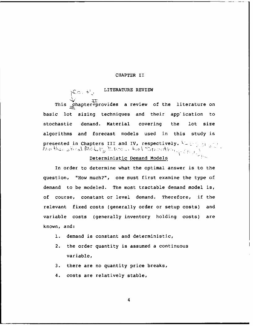
This chapterprovides a review of the literature on

basic lot sizing techniques and their app'ication to

stochastic demand. Material covering the lot size

algorithms and forecast models used in this study is

presented in Chapters III and IV, respectively. ' -.

Deterministic Demand Models -

In order to determine what the optimal answer is to the

question, "How much?", one must first examine the type of

demand to be modeled. The most tractable demand model is,

of course, constant or level demand. Therefore, if the

relevant fixed costs (generally order or setup costs) and

variable costs (generally inventory holding costs) are

known, and:

1. demand is constant and deterministic,

2. the order quantity is assumed a continuous

variable,

3. there are no quantity price breaks,

4. costs are relatively stable,

4

5

5. replenishment/production lead time is zero, and

6. no shortages or back orders are allowed,

the optimal (most economic) production or order quantity is

easily derived by minimizing the total relevant costs (TRC)

per unit time, i.e.,

TRC(Q) = variable cost + fixed cost Q h/2 + A D/Q

where Q is the order or production quantity, h is the

inventory holding cost expressed as cost per unit per

period, or $/unit/period, A is defined as the fixed set-up

or order cost, and D is the demand rate of the item in

units per unit time (from Silver and Peterson, 1985).

Specifically, this economic order quantity, or EOQ, is

given as:

EOQ = (2 A D / h)f

Once we relax the assumption of level demand and allow

time variance, however, the EOQ is no longer guaranteed to

provide an optimal solution.

This assumption of constant demand is one of the first

problems we encounter with the basic EOQ model. Few

manufacturers, suppliers, or retailers can expect to have

requirements for exactly N units of a product every period

6

over the entire product's life cycle. In fact, one would

expect demand to (hopefully) increase from zero when a

product is introduced, stabilize once initial demands are

satisfied, and then (unfortunately) decrease as the product

becomes obsolete. And, generally, this is the case.

Hofer (1977) defines the fundamental stages of

product/market evolution similarly. However, all stages

basically fall into three categories: linearly increasing

demand, level demand, and linearly decreasing demand

(Chalmet, De Bodt, and Van Wassenhove, 1985). These time

varying levels of demand render the once optimal EOQ model

to the level of a mere heuristic. (A heuristic is an

algorithm which gives near optimal problem solutions.)

Although the Wagner and Whitten (1958) dynamic

programming approach to the time varying demand model is

guaranteed to provide an optimal solution, many authors

feel this method is too complicated for general industrial

use (McLaren, 1977; Silver, 1981; Wagner, 1980). In

addition, the Wagner-Whitten algorithm may provide

sub-optimal results when used in the context of a rolling

demand horizon as normally used in industry (De Bodt and

Wassenhove, 1983a). This "sub-optimality" results from

violation of the assumption that demand after the last

period in the horizon is zero. It is interesting to note,

however, that objections to use of the Wagner-Whitten

technique have steadily declined in the past several years

7

primarily due to the general increase in the power of

microcomputers and the advent of such efficient high level

languages as C and PASCAL (Saydam and McKnew, 1987 ; Evans,

1985).

As a result, most work in this area has involved the

development, test and evaluation of a multitude of

(generally) simple heuristic policies in an attempt to

provide solutions as "near-optimal" as possible. Some of

these heuristics include EOQ, Silver-Meal, part-period

balancing (Eisenhut), and least total cost to name a few.

All heuristics can be divided into three general

classifications, specifically:

1. EOQ rules (which trade off order costs and

holding costs per unit time, e.g., discrete EOQ),

2. Marginal cost rules (which equate marginal

order and holding costs per period, e.g.,

Silver and Meal, 1973), and

3. Target rules (which set holding costs equal to a

target, e.g., the part-period balance algorithm

which increases the production lot size until the

holding cost reaches a target equal to the

ordering cost)

(From Wemmerl6v and Whybark, 1984).

Several studies have shown that various heuristics

will perform differently under different types of

conditions. In particular, Ritchie and Tsado (1986) have

8

shown the best, most robust lot-size heuristics to be

marginal cost (Groff, 1979), the simplified part-period

(balance), and Silver-Meal algorithms. Further, they show

that switching from one rule to another is not worthwhile,

meaning it is generally better to use a good rule to begin

with.

Therefore, given deterministic, time varying demand,

the question of how much to produce or order seems to be

relatively easy to answer. Unfortunately, we encounter a

second problem with our assumptions on demand.

One rarely knows with any certainty what future demands

will be (Tsado, 1985a).

Stochastic Demand Models

Solution of the EOQ or lot size problem for stochastic

demand is very difficult. As a result, most research in

this area has focused on the relative performance of

algorithms designed for deterministic demand as applied to

stochastic demand over a rolling horizon (Benton and

Whybark, 1982; Callarman,1979; Callarman and Hamrin, 1979,

1984; De Bodt and Wassenhove, 1983; Tsado, 1985a; Wemmerl6v

and Whybark, 1984).

By rolling horizon, we mean that "lot sizing takes

place over a fixed number of periods, the forecast horizon,

and that only the first period's decision is implemented.

Next period, a new fixed horizon problem is made, etc.

(Baker and Peterson, 1979)." (From Wemmerl6v and Whybark,

9

1984.) The forecast horizon, in turn, is based on mean

time between orders, or TBO, given by:

I

TBO ((2 A)/(D h)]2

where A is the setup or holding cost, D is the average

forecasted demand, and h is inventory holding cost. TBO,

therefore, is dependent on the inventory ratio, i.e., A/h.

There is no one consensus on what values of A/h to

use. In a problem presented by Berry (1972) and later used

by many others, the value was 152.5. De Matteis (1968),

on the other hand, used a factor of 100. (From Heemsbergen,

1987.) Tsado (1985) used a wide range of values,

specifically:

7.5 10.0 30.0 50.0 70.090.0 110.0 130.0 150.0 170.0

Ritchie and Tsado (1986) used a value of 400! The reasons

why the literature is so inconsistent are not quite clear,

however the reasons for using such a broad range are.

DeBodt and Van Wassenhove (1983) have shown that various

ranges of TBOs will lead to different costs even when

forecast error is small. Specifically, smaller values of

TBO lead to larger percentage cost increases. Studies by

Blackburn and Millen (1980) suggest that a forecast horizon

of 3 TBO is sufficient to minimize cost increases due to a

small forecast horizon, but only for heuristic procedures.

10

Due to the sensitive nature of the Wagner-Whitten

algorithm, Lundin and Morton (1975) suggest a forecast

horizon of 5 TBO to ensure a cost performance that is

within 1% of the "optimal" for an infinite horizon

(Wemmerl6v and Whybark, 1984).

Callarman and Hamrin (1979), in one of the earliest

studies of stochastic demand, compared the relative

performance of six well-known heuristics (such as the EOQ,

part-period, and Silver-Meal algorithms) under conditions

of uncorrelated forecast errors and fixed lead times while

using the coefficient of demand variation (s/m) and time

between orders (TBO) as experimental factors. Their basic

conclusion was that no single lot sizing rule was "best"

under all conditions. They did rank the heuristics,

however, with Wagner-Whitten coming out on top, followed

closely by the EOQ, and ending up with Silver-Meal as one

of the poorer performers. They also noted that total costs

tended to increase with forecast error resulting in smaller

differences in the relative performance of the heuristics.

Callarman (1979) reaffirmed these results for an inventory

model which, unlike the previous study, explicitly included

stockouts. (From Tsado, 1985a, and Wemmerl6v and Whybark,

1984.)

Benton and Whybark (1982) confirmed the results of

Callarman (1979) and Callarman and Hamrin (1979).

Specifically, their study of three lot sizing techniques

11

(using uncorrelated forecast errors and varying such system

parameters as level of uncertainty), showed a negative

correlation between relative heuristic performance (in

terms of cost) and forecast error, i.e., as forecast error

increased, the differences in cost performance of the three

heuristics decreased. (From Wemmerl6v and Whybark, 1984.)

De Bodt and Wassenhove, in two separate studies,

reported findings similar to those previously mentioned.

Their first study (1981) examined the relative performance,

both analytically and via simulation, of the

Wagner-Whitten, Silver-Meal, and least unit cost

algorithms. Using simulated constant demands injected

with white noise and forecasted using exponential

smoothing, they showed that cost differences were

negligible even when the amount of forecast error was

small. Although the assumptions on demand were rather

restrictive, the simulation results bore out the analytical

results regarding expected cost increases due to forecast

error.

Their second study (De Bodt and Van Wassenhove, 1983a)

used actual demand data but was also a simulation effort in

that the forecast error was generated artificially. Their

conclusions were essentially the same (i.e., Silver-Meal,

part-period, least unit cost, and EOQ, adjusted to cover

integral periods of demand, performed equally well),

however they did state a preference for the basic EOQ model

12

when used in a multi-stage environment. These results are

interesting in that some of the operating conditions were

different from those used in earlier research.

Specifically, the authors assumed zero lead time and that

the forecast error for the next period's demand was zero

(implying zero probability of a stockout). These

assumptions were made in order to make the analytical study

tractable.

The following year, Wemmerl6v and Whybark (1984)

presented a comprehensive study of 14 single-stage lot

sizing techniques using demand uncertainty in the form of

forecast errors introduced via simulation. The operating

conditions are similar to those used by Benton and Whybark

(1982), Callarman (1979), and Callarman and Hamrin (1979).

However, they do incorporate non-zero lead times. Their

most important results are quoted as follows:

"l. Relative cost performance is strongly affected bythe introduction of forecast errors. The magnitudeof these errors, however, is not significant.

2. The Wagner-Whitten procedure loses its position asthe least cost rule (as in the deterministicdemand model).

3. Only two rules, [Wagner-Whitten] and WMR3[suggested by Wemmerl6v (1981)], remain on thelist over the six best rules overall (from thelist of best performers in the deterministicdemand model).

4. The relative advantage of [Wagner-Whitten]compared to the other rules decreases.

13

5. The performance of the EOQ rule improvesdramatically. This is, no doubt, due to thenon-discrete character of this rule, leading tothe ordering of a larger quantity than what isneeded over an integer number of periods. Ineffect, then, the EOQ rule carries with it its ownsafety stock.

6. A wider choice of lot-sizing rules is availablewhen compared to the 'no uncertainty' case. Notonly are there no differences, from a statisticalstandpoint, among the six best rules, but the costpenalties for several of the other heuristics arequite small. This can be contrasted to the casewith no demand uncertainty, for which (Wagner-Whitten)... emerge[s] as being significantlybetter than the other rules."

They further point out that their simulation results

seem to justify current industry practice. Specifically,

Wagner-Whitten is not applied in industry (primarily due to

complexity and "system nervousness" as shown in their

study). The EOQ and Eisenhut algorithms, on the other

hand, are widely used. Previous studies involving

deterministic demand would lead one to believe this is bad

practice. However, "if it is acknowledged that the

'forecasts are always wrong', then current industry

practice seems to be justified." In other words, the

question of which lot sizing technique is the "best"

becomes moot; a simple technique will probably suffice.

Tsado (1985a) concurs with the results of Wemmerl6v and

Whybark (1984). However, he recognizes a serious

limitation to their work and to the work of those that

preceded them. All of these studies involved the use of

simulated demand data and/or simulated forecast errors.

14

"While simulation is an important tool for analysingproblems that requires (sic) complex mathematicalsolutions, it could lead to different results bydifferent users, if there are differences in the waythe data was simulated, or in the demandcharacteristics of the data. Moreover, simulationscannot always explain all the peculiarities of reallife experience."

Additional problems with the previous works are:

1. Each study uses different versions of the

part-period balance (see Heemsbergen, 1987).

2. There were contradictions in some of the initial

assumptions (discussed previously).

3. All forecast errors were assumed to be unbiased.

However, in actual practice forecasts may be

biased.

4. Forecasting techniques (exponential smoothing,

regression, etc.) were not used.

Tsado's (1985a) study therefore attempted to examine

the possible interactions between demand pattern and lot

size performance, lot-size technique and forecasting

technique (or forecast parameters), and uncorrelated

forecast errors and lot-size performance. His results

follow:

"1. Forecast errors have tremendous influence onthe performance of the heuristic policieseven when these forecast errors are small.

2. With the exception of the incremental costapproach, the cost differences between anumber of heuristic policies is small. Thiscontrast(s) with the case of deterministictime varying demand function for which there

15

were significant differences between theperformance of the heuristic policies.

3. The magnitude of the trend in demand and thetype of forecasting technique used seem tohave insignificant influence on performance .... "

Tsado (1985a) hoped to validate the previous work on

lot-sizing techniques (as well as compare his own heuristic

developed specifically for stochastic demand), and, on the

surface, it appears that he did. In the case of simulated

data, he used (linear) exponential smoothing. He broadened

his scope on the published data by including the use of

Winter's seasonal forecasting model. He restricted his use

to (linear) exponential smoothing once again for the actual

demand data. His reasoning was that "these forecasting

methods were (appropriate) because they provided reasonable

forecasts." Unfortunately, Tsado limited his application

of these forecasting techniques by using the entire demand

history available to him to fit his forecast.

Industry, on the other hand, does not have this

ability. In other words, forecasts are based on a limited

demand history (if at all) and are then updated

continuously over the "rolling horizon", i.e., from period

to period. Tsado's methods therefore do not seem

reasonable. What methods, then, are reasonable?

Makridakis, Andersen, Carbone, Fildes, Hibon,

Lewandowski, Newton, Parzen, and Winkler (1982) established

the following:

16

1. Knowledge of the underlying demand pattern of a

time series does help in choosing a model.

2. Simple models seem to work well, especially when

the basic series is changing or in the absence

of prior knowledge as to the underlying

structure of the demand pattern.

3. Under the conditions where simple models work well,

the average of the forecasts from several simple

models was superior to the forecast from a single

model.

Flores and Whybark (1986), however, proposed a

different method. A practitioner developed approach, this

method, called focus forecasting, involves the selection of

the one forecasting model which would have performed the

best in the recent past to make the next forecast. As a

result of continuous updating of all forecasting models,

the choice of forecasting method may vary from time to

time.

They compared both techniques (average vs. focus

forecasting) using both synthetic (simulated) and empirical

(actual) demand data. The method of averaging performed

best on the synthetic data. More importantly, there was no

significant difference in the relative performance of for-us

forecasting and forecast averaging when used on empirical

data. The authors believe this is due to the higher mean

17

average deviations (MADs) characteristic of actual demand.

In other words, "empirical time series are far more

difficult to forecast than the synthetic".

It is important to note that none of the seven

forecasting techniques used for both focus forecasting and

forecast averaging used any form of regression, exponential

smoothing, Winter's method, or ARIMA modeling (although a

simple moving average of 3 and 6 months was used). They

did, however, compare the focus and averaging techniques

with exponential smoothing (as a common basis of

comparison) and observed that exponential smoothing

generally outperformed both although the significance was

not as great for the empirical demand data. It would

therefore be interesting to apply focus forecasting to the

more sophisticated exponential smoothing models.

Additionally, all of the aforementioned studies

combined shortage costs with inventory holding and setup

costs. (Some authors incorporated an arbitrary service

level using a predetermined amount of safety stock.)

Wemmerl6v and Whybark (1984) point out two approaches. One

is to set stockout costs as a separate factor. However,

they state that the results might not be meaningful when

compared to other studies. The other, used by all of the

studies cited, sets service levels via an appropriate

amount of safety stock and quantifies only the inventory

holding and setup costs.

18

A basic assumption for this method to be valid is that

the "cost" of a stockout is the same for everyone. Another

is that each heuristic employed performs the same for

relative shortage costs as they do for relative inventory

costs. These assumptions may not be valid, therefore it

may be appropriate to look at these two types of costs

separately.

Bookbinder and H'ng (1986) employed both forecasting

methodology and stockout costs (separate from the standard

inventory costs) in their study of rolling horizon

production planning. Their main emphasis, however, was on

the procedure for probabilistic production planning and not

on the relative performance of the lot sizing rule employed

within the procedure.

And finally, the baseline used in the previous studies

on lot size algorithms to determine relative cost increases

for each heuristic is questionable. Most of these works

(including Wemmerl6v and Whybark, 1984) used the

WagnerWhitten heuristic (i.e., given stochastic demand) as

the baseline. Tsado (1985a) employed the EOQ "heuristic".

But this is like trying to measure distance with a rubber

ruler!

It is suggested that, in order to minimize the "error"

inherent in such an approach, the optimal Wagner-Whitten

solution given a-priori knowledge of the demand "history"

19

should be used. The increase in cost due to the heuristic

using forecast demand can then be thought of as the

expected value of perfect information (EVPI). EVPI may be

thought of as the maximum amount of money one would be

willing to pay for perfect knowledge of the future. This

approach should not only minimize the error in the design

model, but should also be intuitively more appealing. (See

Raiffa, 1968.)

Research Goals

There is a need for a study which forecasts empirical

demand in the same manner ir iiich the lot sizing

algorithms are implemented, i.e., over a rolling horizon.

For the purposes of this study, a system of focus

forecasting is used.

Further, shortage costs need to be analyzed separately

from inventory and setup costs since (1) shortages have

a "variable" cost, and (2) the various algorithms may

perform differently when shortages are treated as a

separate entity.

Finally, validation of the stochastic heuristic

presented by Tsado (1985a, b) is required.

CHAPTER III

LOT SIZE HEURISTICS

The lot size heuristics described are those developed

for deterministic or discrete demand. As stated, there are

three basic categories of lot size algorithms: EOQ-based,

marginal cost-based, and target-based. The algorithms used

in this study for each category are the standard EOQ,

Silver-Meal, and part-period balance methods, respectively.

Also presented are Wagner and Whitten's (1958) dynamic

programming method which is used as both an optimal

baseline for cost comparison and as a separate lot size

heuristic (when solved for forecast demand) and Tsado's

(1985a, b) stochastic lot size heuristic. Although various

refinements exist for all the heuristics listed, the

simpler versions were used in the study.

Eisenhut

The part-period balance algorithm, hereinafter referred

to as Eisenhut's lot size heuristic, determines the number

of periods to order or produce by selecting that period for

which holding cost most closely approximates the setup

20

21

or ordering cost.

Using the example provided by Silver and Peterson

(1985), let the setup cost = $54, holding cost = $0.40 per

unit per period, and demand be given by Di = {10, 62, 12,

130, 154, 129) for the first 6 periods. The algorithm

yields

T=I: Holding = 0

T=2: Holding = D2 h = $24.80 < $52.00

T=3: Holding = $24.80 + 2D3h = $34.40 < $52.00

T=4: Holding = $34.40 + 3D4h = $190.40 > $54.00

Therefore since

134.40 - 52.001 = 17.60 < 152.00 - 190.401 = 138.40

we produce for 3 integral periods.

EOQ

The economic order quantity, derived earlier, is

non-optimal for the case of non-constant, or time-varying,

demand. To be used as a heuristic in the case of

stochastic demand, the average of the forecasted demand is

used in the model.

Using the same example where Di is a 6-period

forecast, average demand is approximately 83 units.

Therefore

22

Q = (2 x 52.00 x 83 / 0.40)2 = 147 units

where Q* is the "optimal" order quantity defined by the

standard EOQ formula. Notice that the simple form of EOQ

provides a non-integer time supply which, in effect, acts

as an automatic safety stock (Tsado, 1985a).

Silver-Meal

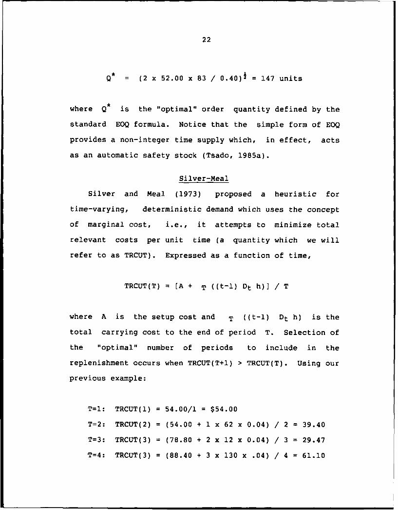
Silver and Meal (1973) proposed a heuristic for

time-varying, deterministic demand which uses the concept

of marginal cost, i.e., it attempts to minimize total

relevant costs per unit time (a quantity which we will

refer to as TRCUT). Expressed as a function of time,

TRCUT(T) = (A + T ((t-l) Dt h)] / T

where A is the setup cost and T ((t-l) Dt h) is the

total carrying cost to the end of period T. Selection of

the "optimal" number of periods to include in the

replenishment occurs when TRCUT(T+I) > TRCUT(T). Using our

previous example:

T=I: TRCUT(1) = 54.00/1 = $54.00

T=2: TRCUT(2) = (54.00 + 1 x 62 x 0.04) / 2 = 39.40

T=3: TRCUT(3) = (78.80 + 2 x 12 x 0.04) / 3 = 29.47

T=4: TRCUT(3) = (88.40 + 3 x 130 x .04) / 4 = 61.10

23

and we select a replenishment quantity which will cover 3

periods.

Tsado

Tsado's (1985a) stochastic heuristic is primarily a

modification of the EOQ which incorporates the idea of

minimizing total relevant costs for a given replenishment

cycle while keeping track of previous costs. As this

method is generally unknown, more will be said regarding

its derivation.

The assumptions used in the derivation are (1) no

shortages are allowed, (2) demand for the next period is

known with certainty, (3) all other periods are forecast,

(4) a replenishment occurs in period t if demand cannot

be satisfied for period t+l, and (5) demand is assumed to

be steady and continuous. The first two assumptions are

basically equivalent and neither is used in this research,

i.e.,, we allow shortages.

Tsado (1985a) first derives an equation for the

expected increase in stockholding costs, Stc, given that

(1) lead time is zero, (2) replenishment occurs

instantaneously, and (3) stock at the end of the

replenishment interval is zero. Specifically,

Stc = h D L2 / 2

24

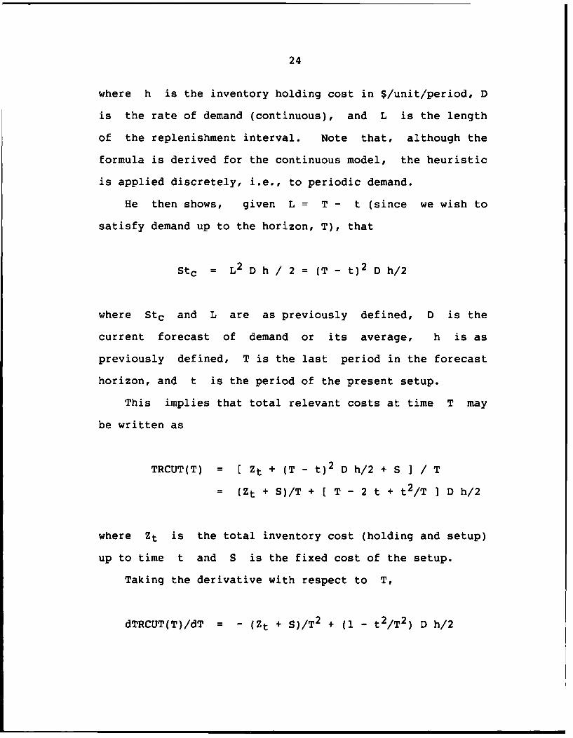
where h is the inventory holding cost in $/unit/period, D

is the rate of demand (continuous), and L is the length

of the replenishment interval. Note that, although the

formula is derived for the continuous model, the heuristic

is applied discretely, i.e., to periodic demand.

He then shows, given L = T - t (since we wish to

satisfy demand up to the horizon, T), that

Stc = L2 D h / 2 = (T - t) 2 D h/2

where Stc and L are as previously defined, D is the

current forecast of demand or its average, h is as

previously defined, T is the last period in the forecast

horizon, and t is the period of the present setup.

This implies that total relevant costs at time T may

be written as

TRCUT(T) = [ Zt + (T - t) 2 D h/2 + S ] / T

= (Zt + S)/T + [ T - 2 t + t2 /T ] D h/2

where Zt is the total inventory cost (holding and setup)

up to time t and S is the fixed cost of the setup.

Taking the derivative with respect to T,

dTRCUT(T)/dT = - (Zt + S)/T 2 + (1 - t2/T 2 ) D h/2

25

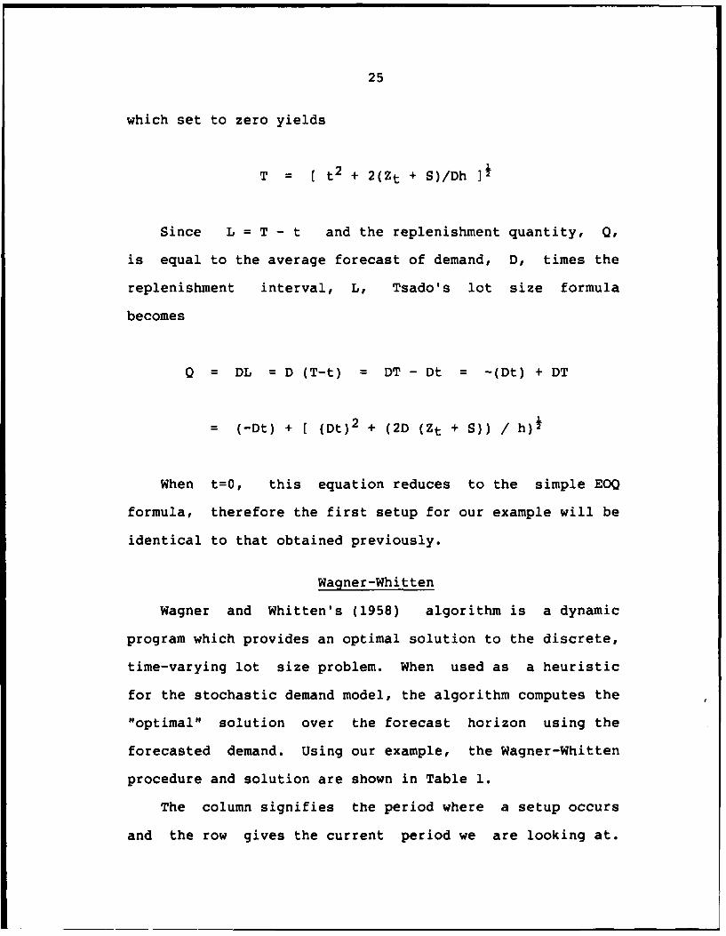
which set to zero yields

T = [ t2 + 2(Zt + S)/Dh ]2

Since L = T - t and the replenishment quantity, Q,

is equal to the average forecast of demand, D, times the

replenishment interval, L, Tsado's lot size formula

becomes

Q = DL = D (T-t) = DT - Dt = -(Dt) + DT

= (-Dt) + [ (Dt)2 + (2D (Zt + S)) / h)2

When t=O, this equation reduces to the simple EOQ

formula, therefore the first setup for our example will be

identical to that obtained previously.

Wagner-Whitten

Wagner and Whitten's (1958) algorithm is a dynamic

program which provides an optimal solution to the discrete,

time-varying lot size problem. When used as a heuristic

for the stochastic demand model, the algorithm computes the

"optimal" solution over the forecast horizon using the

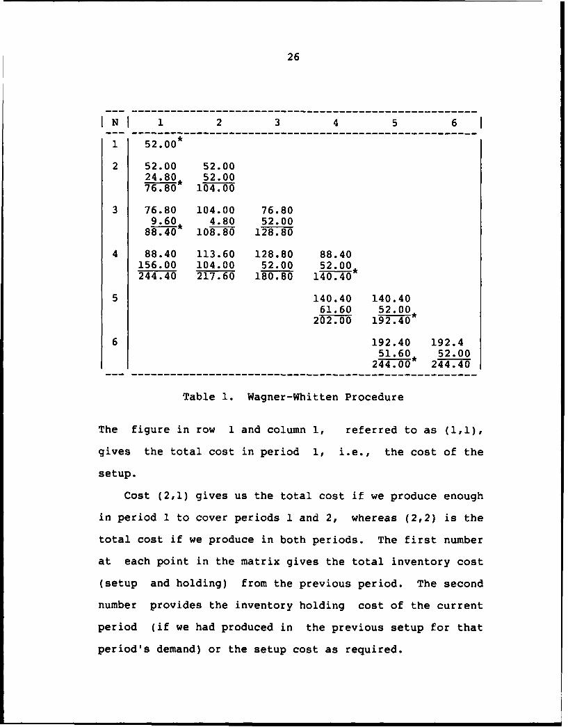
forecasted demand. Using our example, the Wagner-Whitten

procedure and solution are shown in Table 1.

The column signifies the period where a setup occurs

and the row gives the current period we are looking at.

26

IN! 1 2 3 4 5 6

1 52.00*

2 52.00 52.0024.80* 52.00768i 104.00

3 76.80 104.00 76.809.60* 4.80 52.00

88.4i 108.80 128.80

4 88.40 113.60 128.80 88.40156.00 104.00 52.00 52.00244.40 217.60 180.80 140.40*

5 140.40 140.4061.60 52.00*

202.00 192.40

6 192.40 192.451.60* 52.00

244.0 244.40

Table 1. Wagner-Whitten Procedure

The figure in row 1 and column 1, referred to as (1,1),

gives the total cost in period 1, i.e., the cost of the

setup.

Cost (2,1) gives us the total cost if we produce enough

in period 1 to cover periods 1 and 2, whereas (2,2) is the

total cost if we produce in both periods. The first number

at each point in the matrix gives the total inventory cost

(setup and holding) from the previous period. The second

number provides the inventory holding cost of the current

period (if we had produced in the previous setup for that

period's demand) or the setup cost as required.

27

The asterisk shows the "optimal" policy for the current

period, and, except for the policy where we "test" for a

setup (which is given on the diagonal), that cost is

carried over to the next period we wish to look at (every

(i,j) "period" where j < i).

The Wagner-Whitten theorem states that, once the

optimal policy occurs in column j, calculations may be

discontinued for any column i where i < j.

In general, a cost C(i,j), means that we set up in

period j to produce demands for periods j, j+l,..., i,

and that the demands for periods 1, 2,..., j-1 are

produced by an optimal policy.

Unlike the previous heuristics, the Wagner-Whitten

algorithm must be used over the entire forecast

(time-rolling) horizon, but, like the others, only the

first period's decision is implemented. Cost calculations

are carried out in the same manner as in the other

heuristics.

The "optimal" Wagner-Whitten solution is read backwards

through the matrix using the "starred" costs as a guide.

For our example, we show setups in periods 1, 4, and 5 and

would produce in the first period for periods 1, 2, and 3.

Note that optimality of the Wagner-Whitten procedure is

no longer guaranteed since the assumptions of deterministic

demand and zero demand after period T, where T is the

planning horizon, are violated.

CHAPTER IV

THE FORECAST MODEL

Time series analysis involves developing forecasts of a

variable entirely from its past history. These techniques

generally model the variable in such a way that past

patterns in the data series are used to help modify the

mean and thereby predict future values. Although past

performance is no guarantee of future performance, time

series methods are generally successful in statistically

stable conditions, for short-term forecasts where there is

insufficient time for substantial change barring

catastrophes (as in our current study), as a base forecast

for judgemental models, and for screening data in order to

better understand the variable being forecasted (Barron and

Targett, 1985).

Introduction

Jenkins (1979) describes five classes of time series

models. These are:

1. univariate models in which a single variable is

forecast from its own past history,

28

29

2. transfer function models which add inputs from

other variables,

3. intervention models which represent unusual events

such as strikes, etc.,

4. multivariate stochastic models which represent

several series with mutual interaction, and

5. multivariate transfer function models which

relate several output variables to several input

variables in which a relationship exists.

Univariate models, although of an elemental nature, are

important from a forecasting viewpoint for several reasons.

First, they may be the only model which is the only

practical approach based on the magnitude of the problem.

Second, ',it may be impossible to find, or there may not

exist, variables related to the one being forecast. Third,

when multivariate models exist, the univariate model may be

used as a baseline to measure the other's performance. And

finally, the presence of large residuals (the difference

between actual values and the "stationary mean") may

correspond to strikes, faulty data, etc. and therefore act

as a tool to screen data. In spite of these points,

30

however, it must be recognized that univariate models are

generally valid for short-term forecasts only (Ibid.). As

all of the studies mentioned in Chapter II utilized

univariate forecasting methodology, this discussion will

be restricted to procedures in this area.

Univariate models are classified by Barron and Targett

(1985) according to the type of series to which they can

be applied. These are:

1. stationary (random variation about a mean or a

series which may be modeled as a stochastic

"random walk"),

2. trending (a consistent movement either upwards or

downwards in the series),

3. seasonal/cyclical (a series which exhibits a

pattern over a number of time periods where

seasonal implies a period of a year or less and

cyclical refers to a pattern greater than one

year), and

4. seasonal and/or cyclical with a trend (a complex

of seasonal and/or cyclical patterns and trends).

31

The last three classifications may be grouped under the

heading of non-stationary time series. Johnson and

Montgomery (1976) state that the basic goal in any

univariate time series method is to reduce the residuals,

or error, to a normally distributed random variable with

mean zero and constant variance (also known as "white

noise"). In other words we seek a stationary model from a

non-stationary time series. (See Hoel, Port, and Stone,

1972.)

There are two general types of time series forecast

methods, those involving smoothing techniques and those

involving autoregressive parameters, generally referred to

as ARMA (p,q) models. Johnson and Montgomery (1976)

suggest that ARMA models should be considered only when

there exists a sufficient amount of demand history for

analysis, typically around 36 periods or more. Since large

amounts of demand history from the same environment may not

always be available and previous studies have not utilized

ARMA models, ARMA models were not considered for use in the

current study.

Further, since lot sizing is performed on a rolling

horizon, forecasting should be performed on the same basis.

Therefore, we will restrict ourselves to exponential

smoothing models when applied to the concept of focus

forecasting.

32

Exponential Smoothing

Smoothing techniques (or models) replace the original

time series by a "smoothed" one, i.e., one produced from

statistical or weighted averages of values from the

original series in an attempt to reduce or discount the

random fluctuations or variance. Generally, the last

smoothed value(s) provide(s) the forecast for all future

time periods in the (rolling) forecast horizon.

Simple Exponential Smoothing Model

The simplest case is, of course, when the time series

is already stationary, i.e., it may be represented by

xt = m + et

where m (or mu) is the statistical mean of the time

series and et is the error or difference between the mean

and the actual value of the data point. Two techniques

which deal with such stationary models are moving averages

(not discussed) and simple exponential smoothing.

Exponential smoothing assumes that recent data is more

important than old data; a concept which is rather

intuitively appealing. Then, based on the relative value

attached to the significance of the residuals, it computes

a smoothed "average" of the data. Specifically, the model

states

33

St = (1 - a) St_ 1 + a xt

where St is the new smoothed value at time t, St_ 1 is

the old smoothed value at time t-l, xt is the most

recent actual value, and a (or alpha) is a weight chosen

by the forecaster such that 0 < a < 1. Obviously, the

larger the value of alpha the more weight will be attached

to the most recent data point.

To see this, one merely needs to expand the equation

for all "N" which yields

St = a xt + a (1-a) xtl + a (1-a) 2 xt_2 + ---

where the weights given to the data points from the most

recent to the most distant are a, a (1-a), a (1-a)2 , and

so forth (Barron and Targett, 1985). Since both a and

(1-a) are less than one, the weights are decreasing

monotonically with time.

Silver and Peterson (1985) rewrite the exponential

smoothing model to obtain

St = St- 1 + a (x(t) - St-l) = St- 1 + a et

where all variables are as previously defined. This

implies the new forecast value is equal to the old forecast

34

value minus a fraction of the most recent error. In other

words, the exponential smoothing model assumes that a

portion of the last forecast error, namely (1-a) is due to

some random fluctuation and the other portion, namely

alpha, is due to some real shift in the value of the

estimate. In practice, the value of alpha usually ranges

between 0.1 and 0.4 (Ibid.).

Holt's Exponential Smoothing Model

Now consider time series which are initially

non-stationary but which can be made stationary by

differencing. By differencing we mean

DEL St = St - St-d

where DEL is the differencing operator and d is the

period of differencing. For a strictly trending time

series, a difference of d=l will yield a stationary time

series.

To see this, one must first examine the statistical

significance of trending and seasonal data. When a time

series trends, the values between successive data points

are highly correlated. (Since the time series is

correlated with itself, a more appropriate term is

"autocorrelated".) The same is true for seasonal time

series where the autocorrelation occurs at lag d, i.e.,

for time series values St and St- d . The differencing

35

operator therefore yields white noise, i.e., the residuals

are normally distributed with zero mean and constant

variance (Jenkins, 1979). As mentioned earlier, the

objective of all time series analyses is to fit a model

such that the residuals yield white noise (Johnson and

Montgomery, 1976).

Due to the nature of how the forecasting methodology

was implemented, exponential smoothing models which account

for seasonality were ignored. Trend, however, is accounted

for through the use of Holt's exponential smoothing model.

(Linear regression may also be used buL was not employed in

this study.)

A strictly trending (linear) time series will take the

form

xt = m+Bt +et

where Bt defines a linear trend (as a function of t)

with slope 1. Other trends are possible. However, our

discussion is limited to linear trends. Successfully

differencing a time series more than once for trend is a

good indication the trend is non-linear (Ibid.).

Let the trend at time t be given by Tt = St - St I .

Since St is a random variable, Tt is also a random

variable. Therefore, using the same logic as simple

36

exponential smoothing, we can smooth the trend by the

following:

Tt =(1 - g) Tt_1 + g (xt - Xt-l) )

i.e., the smoothed trend is equal to a portion of the

previous smoothed trend plus a portion of the most recently

observed trend. The selection of g (or gamma) is made in

the same manner as alpha.

Using this estimate, we can modify St_ 1 in the simple

exponential smoothing model to obtain

St = (1 - a) (St_1 + Tt.l) + a xt

or more generally

Ft+i = St + i Tt

where Ft+i is the forecast for the t+i'th period

(Barron and Targett, 1985)

Focus Forecasting

Flores and Whybark (1986) studied two forecasting

systems, "one recommended by practitioners for use in

inventory management, and the other the result of an

37

international forecasting competition among academics."

These are the methods of focus forecasting and forecast

averaging, respectively.

Although this topic was touched upon briefly in the

literature review, we would like to say a little more

regarding the aforementioned study and our proposed

extension.

The forecast procedures used in the comparison were

very simplistic, e.g., "the forecast for the next month is

the actual demand for the same month last year .... [or]

...is one-sixth of the total actual demand for the last six

months (a two-quarter moving average)." Another, slightly

convoluted approach was "if the demand in the last six

months is more than 2.4 times the demand for the six months

preceding that, the forecast for the next month is

one-third of the demand for the same three month period

last year (i.e., we are starting into the downside of a

seasonal. swing)."

The focus and averaging techniques were then compared

to each other and, most importantly, to exponential

smoothing, i.e., exponential smoothing provided the

"baseline" for comparison.

Although averaging performed better than focus

forecasting on the simulated data (there was no statistical

difference for the empirical data), neither procedure

performed better than exponential smoothing. In fact,

38

exponential smoothing was significantly better than either

of the other two procedures.

Exponential smoothing would then seem to be the obvious

choice. The next question, however, is the selection of

alpha and gamma, i.e., the forecast parameters. Past

studies have "fit" the parameters over the entire demand

history of each empirical data set (when empirical data

were used). Industry, of course, doesn't have this type of

clairvoyance; they would have to take an educated guess

given a limited demand history and monitor the forecast

model to make appropriate changes when necessary. But,

since this study was "automated", we did not have this

"luxury" either.

It therefore makes sense to either (1) average the

exponential smoothing forecasts from varying parameter

levels or (2) use the focus forecasting approach. We

selected the focus forecasting approach as it seems to be

the most appealing (intuitively). The idea is to keep

track of the mean absolute deviation and bias of a set of

exponentially smoothed forecasts and select the one best

forecast for the next planning horizon.

Silver and Peterson (1985), however, argue that

changing the smoothing constants (what they refer to as

"adaptive" smoothing), while having considerable intuitive

appeal, is "not necessarily better than regular,

-- - - -

39

non-adaptive smoothing." (See Ekern, 1981; Flowers, 1980;

and Gardner and Dannenbring (1980)) Specifically, they

feel the resulting forecasts would be excessively

"nervous".

Fortunately, the lot sizing problem only requires use

of an extended forecast about every "TBO" periods. For our

purposes, the focus, or adaptive, approach should be quite

reasonable. In fact, comparisons of the mean absolute

deviation (MAD) for the adaptive procedure to the MADs of

each individual, static procedure (tested during program

development) were quite favorable and tend to support this

position.

Separate research regarding the relative merit of focus

or "adaptive" and averaged exponential smoothing techniques

(as used in automatic forecasting) is probably warranted.

CHAPTER V

THE EXPERIMENT

This chapter ccnstitutes the bulk of this research and

is divided as follows: Sample Data, Assumptions,

Performance Criteria, Computer Model, Experimental Design,

Results, and Analysis. Concluding remarks are contained in

Chapter VI.

Sample Data

Data was obtained from two separate industrial sources.

The first group originally contained 500 data sets

consisting of 52 weekly periods, however only 207 of these

proved suitable for our purposes. Specifically, all data

sets which contained an alphanumeric or zeroes were

discarded. The second group was very limited at 5 data

sets, however each data set consisted of 78 (monthly)

periods.

From the first group of 207, 36 were selected randomly

for the study. They were then classified according to the

coefficient of variation and data type.

The variability of each data set was determined to be

40

41

either low (0 < s/m < 0.5), medium (0.5 < s/m < 1.0), or

high (s/m > 1.0), where s (or sigma) is the standard

deviation. Selection of the "cut-offs" were arbitrary.

Data type consisted of two classifications: linear and

non-linear. The reason for this was two-fold. First, a

relatively small number of data sets were selected for the

study. Second, the forecast model used simple exponential

smoothing as well as Holt's exponential smoothing model for

a linear trend, i.e., it wasn't "designed" to handle a

non-linear demand pattern. It was therefore necessary to

account for the possibility the forecast model would

perform worse for the non-linear case.

An ARIMA "identify" was performed on each data set

using the Statistical Analysis System (SAS) ((c) 1985 by

SAS Institute Inc.) in order to determine which demand

patterns could not be considered level, i.e., as white

noise. A second "identify" using a differencing of 1

determined which demand patterns could be considered

non-linear.

A complete listing of the 36 demand patterns in the

first group is given in Appendix A, however we will discuss

a few selected patterns here.

Figure 1 shows a plot of the first data set. Although

the demand series is generally linear with a relatively

small variance, large outliers occurring at periods 14 and

16 "inflate" the coefficient of variation to 1.49. Outliers

42

Constant/Level DemandExample 1

Number of Units

1000

8001600-/

400'

200

01 5 9 13 17 21 25 29 33 37 41 45 49

Demand per Week

Series

MPloti

Figure 1

43

such as these posed somewhat of a problem for the automatic

forecast model; a procedure discounting such outliers was

developed and will be discussed at a later point in this

chapter.

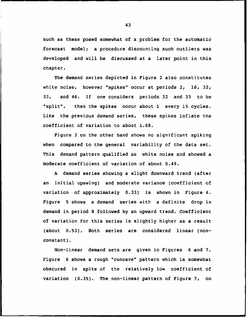
The demand series depicted in Figure 2 also constitutes

white noise, however "spikes" occur at periods 2, 16, 32,

33, and 46. If one considers periods 32 and 33 to be

"split", then the spikes occur about 1 every 15 cycles.

Like the previous demand series, these spikes inflate the

coefficient of variation to about 1.68.

Figure 3 on the other hand shows no significant spiking

when compared to the general variability of the data set.

This demand pattern qualified as white noise and showed a

moderate coefficient of variation of about 0.49.

A demand series showing a slight downward trend (after

an initial upswing) and moderate variance (coefficient of

variation of approximately 0.33) is shown in Figure 4.

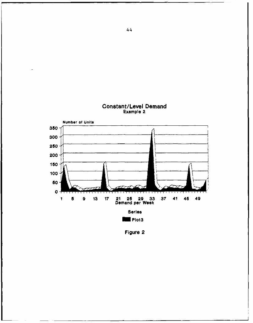
Figure 5 shows a demand series with a definite drop in

demand in period 8 followed by an upward trend. Coefficient

of variation for this series is slightly higher as a result

(about 0.53). Both series are considered linear (non-

constant).

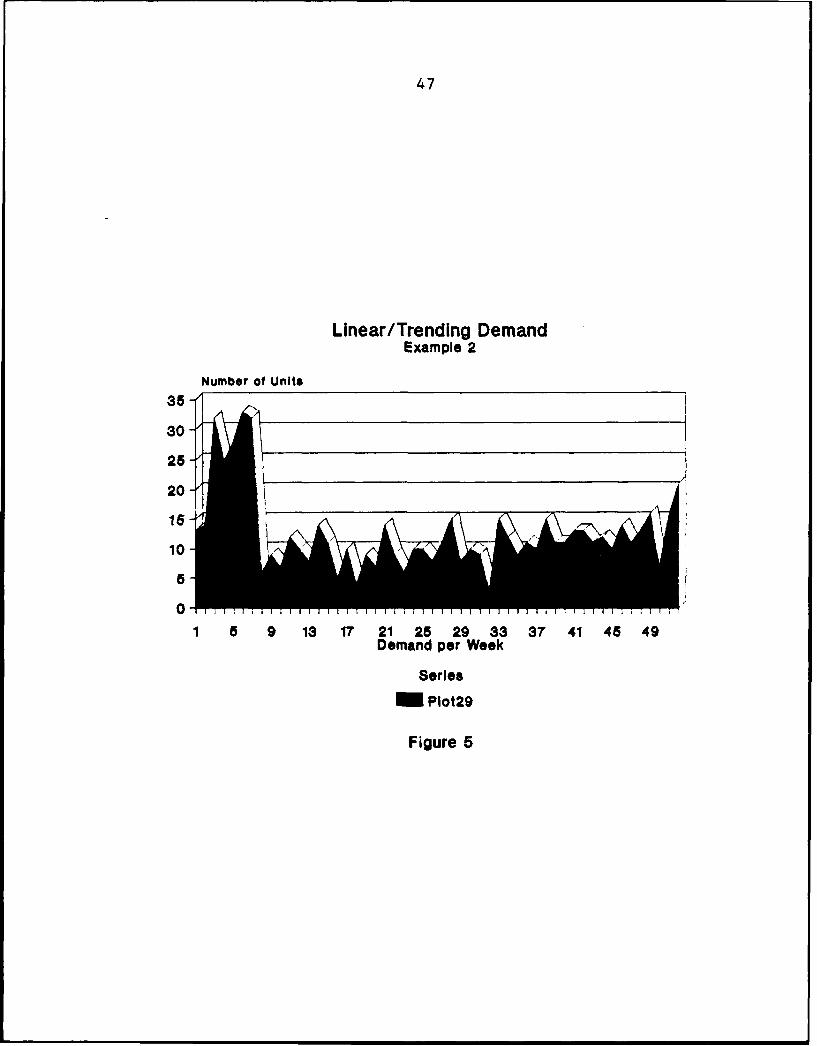
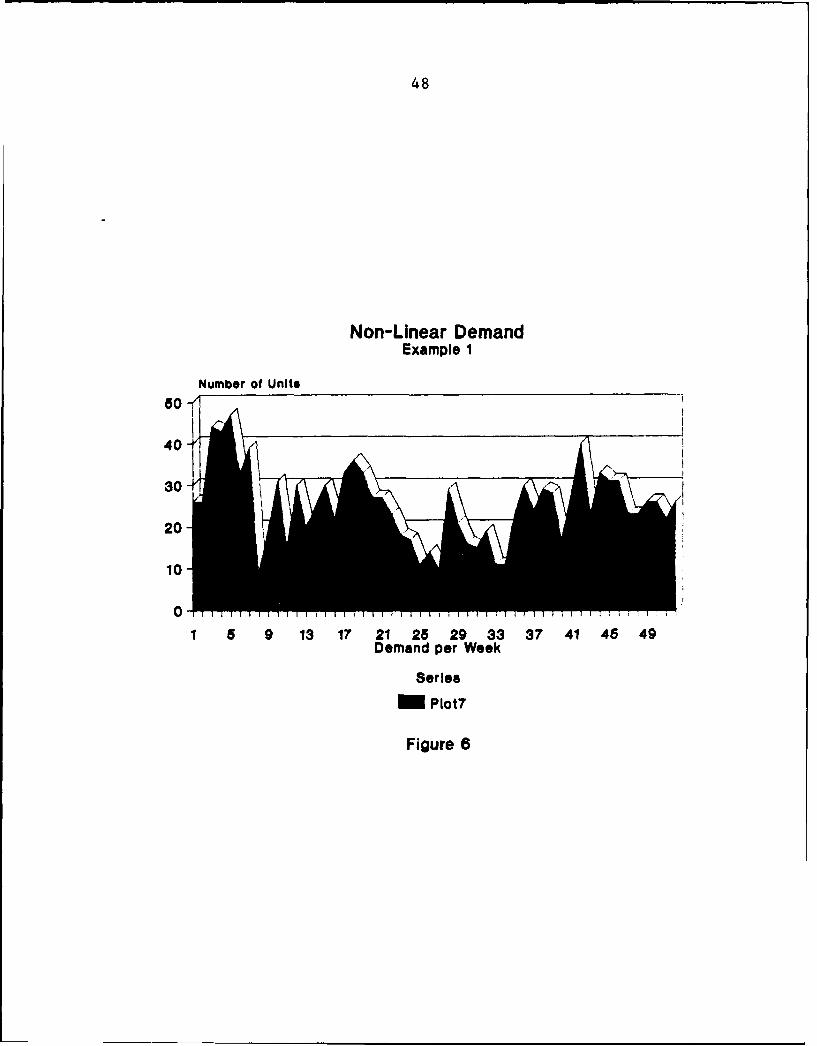
Non-linear demand sets are given in Figures 6 and 7.

Figure 6 shows a rough "concave" pattern which is somewhat

obscured in spite of the relatively low coefficient of

variation (0.35). The non-linear pattern of Figure 7, on

44

Constant/Level DemandExample 2

Number of Units

350

300

250

200

1S0

100

0

1 5 9 13 17 21 25 29 33 37 41 45 49Demand per Week

Series

M Plot3

Figure 2

45

Constant/Level DemandExample 3

Number of Units

80-/

60-/

40

20

01 5 9 13 17 21 25 29 33 37 41 45 49

Demand per Week

Serlee

MPlot4

Figure 3

46

Linear/Trending DemandExample 1

Number of Units40

30

20

10

01 5 9 13 17 21 25 29 33 37 41 46 49

Demand per Week

Series

MPlot6

Figure 4

47

Linear/Trending DemandExample 2

Number of Units35

30

25

20

15

10

0 9

1 5 9 13 17 21 25 29 33 37 41 45 49Demand per Week

Series

M Plot29

Figure 5

48

Non-Linear DemandExample 1

Number of Units

Go

40

30

20

10

0

1 6 9 13 17 21 25 29 33 37 41 45 49Demand per Week

Series

MPlot7

Figure 6

49

Non-Linear DemandExample 2

Number of Units100-

80-

60-'

40

20

0 I

1 5 9 13 17 21 25 29 33 37 41 45 49Demand per Week

Series

MPlot2l

Figure 7

50

the other hand, is clearly convex and could very well be

seasonal (although we can't be sure due to the limited

history). The coefficient of variation for this set is a

slightly higher 0.46.

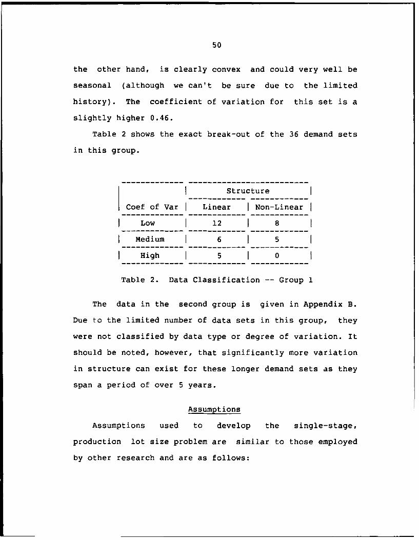
Table 2 shows the exact break-out of the 36 demand sets

in this group.

Structure

Coef of Var Linear I Non-Linear

I Low 1 12 1 8

I Medium 1 6 1 5

I High 1 5 1 0

Table 2. Data Classification -- Group 1

The data in the second group is given in Appendix B.

Due to the limited number of data sets in this group, they

were not classified by data type or degree of variation. It

should be noted, however, that significantly more variation

in structure can exist for these longer demand sets as they

span a period of over 5 years.

Assumptions

Assumptions used to develop the single-stage,

production lot size problem are similar to those employed

by other research and are as follows:

51

1. Demand is probabilistic and is forecast using a

limited amount of prior history.

2. A fixed cost is incurred for each setup.

3. The inventory holding cost is a function of the

amount of inventory on hand at the end of a given

period.

4. Production lead time is zero (i.e., we have enough

inventory at the end of a production period to

meet that period's demand).

5. All demands are met at the end of each period.

6. There is no safety stock except that inherent in

a particular lot size heuristic.

7. Back orders are allowed.

8. There is no monetary penalty for shortages in the

cost calculations (i.e., shortages are handled as

a separate criteria).

9. Demand for the next period is not known with

certainty.

52

10. An updated forecast is available for any period.

Performance Criteria

There are three types of criteria (dependent

variables) of interest in this study. These are cost,

number of stockouts, and the amount short per stockout.

Relative Cost

Previous studies have used the Wagner-Whitten procedure

when used as a heuristic as the baseline for cost

comparisons. Unfortunately, the Wagner-Whitten procedure

is suboptimal in the case of a rolling horizon and

probabilistic demand.

Arguments for the use of the Wagner-Whitten heuristic

as the baseline are:

1. Wagner-Whitten is the baseline used for the

deterministic case.

2. It's not known before hand which rule will

outperform the others.

3. Use of the Wagner-Whitten "heuristic" will make

the study more easily comparable to previous

works.

53

We feel these reasons do not justify the use of one

heuristic as a basis of comparison. It's true that we do

not know what the optimal cost of a probabilistic lot size

problem will be until the demands have already been

satisfied, i.e., we don't know what our future demands will

be. However, by comparing the cost obtained through the

use of a heuristic (when demand is considered stochastic)

with the optimal cost obtained by Wagner-Whitten over the

entire demand "history" (when considered deterministic), we

obtain a true, fixed reference for comparison.

The key is the interpretation of the cost comparison.

Specifically, this difference in cost may be thought of as

the maximum amount of money we would be willing to pay for

perfect knowledge of our future demand (referred to as the

expected value of perfect information or EVPI). (See

Raiffa, 1968.)

Number of Stockouts

Wemmerl6v and Whybark (1984), Tsado (1985a), and others

arbitrarily set service levels in order to handle the

question of stockouts. By service level, we mean that

there exists enough safety stock to assure demands are met

at least percent of the time. Generally, levels

between 90 and 99.999 percent have been chosen. As a

result, the stockout question is largely ignored.

Since we assume that stockouts have a "variable" cost,

i.e., the cost of a stockout to one organization may be

54

quite less than that perceived by another, setting an

arbitrary service level may not be appropriate. Further,

by pre-determining a service level, the effects of a lot

size algorithm on inventory (holding and setup) costs and

stockout costs may be confounded.

In a manner similar to that employed by Bookbinder and

H'ng (1986), we chose to "count" the number of times a lot

size heuristic produced a stockout. Obviously, this number

will vary according to the TBO level, therefore we chose to

compute the stockout "cost" as the number of times a

stockout occurred expressed as a percentage of the number

of replenishments made.

For example, given a 52 period demand "history" with a

TBO level of 2, then 5 stockouts out of 26 replenishments

(approximately) will yield a stockout "cost" of 0.1923,

i.e., about 19.23% of the replenishments made experienced a

stockout. For a TBO of 6, 5 stockouts would imply a "cost"

of 57.69%.

Percent Short per Stockout

Another factor in the stockout question is the amount

of shortage when a stockout occurs. The average number

short per stockout is therefore an important "cost"

consideration, however, an average shortage of N units

doesn't tell us much.

There are two ways of handling this problem. One is to

express the shortage as a percentage of average demand,

55

another is to express it as a percentage of the demand for

the period in which we were short. We chose the later.

Justification for our selection is as follows. Consider

an average demand of 500 units. If we were to have

forecast a demand of 550 units where actual demand was 600

units, then our percentage short is only 8.3% of the actual

demand. If we had used average demand, we would have shown

a shortage of 10%. Now assume an average demand of 50

units. Similarly, assume a forecasted demand of 100 units

and an actual demand of 150 units. But now we show a

shortage of 33.3% of actual demand and a misleading 100% of

average demand.

In both cases the forecast was 50 units greater than

average demand, and actual demand was 50 units greater than

forecasted demand. Obviously, shortage "cost" expressed as

a percentage of actual demand is a more accurate estimate

of the true "cost" associated with a shortage.

Computer Model

Although not a simulation study, a computer model was

used to generate forecasts, compute production policies via

the various lot size heuristics (including the optimal

Wagner-Whitten cost), and to compute the costs associated

with each policy. This section discusses the issues of

program development and validation.

56

Program Development

Both the forecasting procedure and lot size procedure

were automated via a program written in MICROSOFT

QuickBASIC (R) and run on an IBM XT (R) compatible

microcomputer. The program listing is given in Appendix C.

For purposes of clarity, this section is further

subdivided into 2 groups. The first discusses the forecast

algorithm; the second addresses the lot size procedure.

The Forecast Procedure. The complete forecast is

generated over the entire demand history of each data set

(on a rolling horizon basis) prior to implementation of the

lot size procedure. Estimates of level demand and trend

(when Holt's exponential smoothing model is used) are

stored in memory. Although the forecast for each period is

used in the lot size procedure, extended forecasts are only

developed when required by the particular lot size

heuristic employed.

To provide a compact computer algorithm, the simple

exponential smoothing procedure was incorporated into

Holt's procedure by setting the trend parameter, g, to

zero.

Focusing is carried out by keeping track of each

individual or single forecast's mean absolute deviation and

smoothed error tracking signal (bias). (Estimates of the

MAD are also exponentially smoothed.) The forecast with

the best current MAD is selected for the focused model if

57

the bias is within acceptable limits, specifically between

-0.8 and 0.3.

Silver and Peterson (1985) argue that a negatively

biased forecast, i.e., where forecast exceeds demand, is

preferable to a positively biased forecast, i.e., where

demand exceeds the forecast, since being a few items

overstock is preferable to consistently being short

(causing too many premature setups).

Wemmerl6v and Whybark (1984) specifically avoid the use

of biased forecasts by adjusting the average actual demand

per period to equal the average forecast demand per period.

While easily done for simulated demand data, it's generally

not appropriate for empirical demand forecast on a rolling

horizon basis.

Research by Lee, Adam, and Ebert (1987) show that "bias

is the only measure that satisfactorily reflects inventory

carrying cost... [and] only bias displays any reasonable

association with the shortage cost and shortage units .... "

Since carrying cost is caused by over forecasting (what

they refer to a positive bias) and shortage costs are

caused by under forecasting (referred to as negative bias),

the use of an unbiased forecast (as used by Wemmerl6v and

Whybark (1984)) might seem reasonable. The research by

Lee, et al. (1987), however, shows that "the structures of

58

these two component costs may not be symmetrical about the

zero bias level." Unfortunately, they do not provide

guidelines as to what the nominal bias levels may be.

The specific bias levels used in the forecast model

were determined in conjunction with an outlier discounting

criterion. An example data set which exhibited a steep

downward trend due to large upward spikes (outliers) was

used. The steep downward trend was "leveled" somewhat by

discounting the outliers (more on this in a moment) and

then varying the bias criteria in an effort to eliminate a

large series of zero forecasts caused by the initial

"trend". (The data set used is shown in Figure 1.)

Outliers were discounted by keeping track of the

average demand and standard deviation of the series at each

point in the forecast "cycle". If an outlier exceeded 4

standard deviations, the actual demand was reduced to the

mean plus 4 standard deviations for forecast purposes. This

provided a stabilizing influence on the forecast which

otherwise would have to have been provided by human

intervention. On the downside, the forecast model would

lag slightly behind a true shift in the mean of the demand

series. (This type of lag is a standard "penalty" for

exponentially smoothed forecast procedures.)

The Lot Size Procedure. Other than the Wagner-Whitten

algorithm, the other heuristics are simple to use and will

not be discussed here (please refer to Appendix C for more

59

information). Our discussion will be limited to that part

of the procedure which determines our production policy.

Research on lot size procedures has been performed by

Silver (1978), Askin (1981), Bookbinder and Tan (1983), and

Bookbinder and H'ng (1986). Our procedure, while developed

prior to our knowledge of the previous works, is similar to

that suggested by Bookbinder and Tan.

Our procedure is as follows:

1. Use a focus forecast from simple exponential

smoothing and exponential smoothing with trend

models for demands over the rolling horizon.

2. Treat the forecast demands as deterministic and

employ a specific lot size heuristic.

3. If on-hand inventory is positive, the amount

produced will be the amount obtained from the

lot size heuristic minus the on-hand inventory.

4. If on-hand inventory is negative, i.e., a stockout

has occurred, the amount produced will be the

amount obtained from the lot size heuristic plus

the amount backordered.

5. Each period, the on-hand inventory is compared to

60

the forecast for the next period. If our forecast

exceeds our inventory position, we schedule a

setup for the next period, otherwise we continue.

6. When the next period's demand is realized, we

either meet demand or we're short. If a shortage

occurs, a setup is scheduled for the next period,

otherwise we look at next period's forecast

(Step 5).

7. We develop an extended forecast only when a setup

is scheduled.

8. Continue this procedure until we exhaust all

available demand data.

9. Discount the inventory holding cost for all on-

hand inventory used to satisfy demand beyond the

last period in the data set.

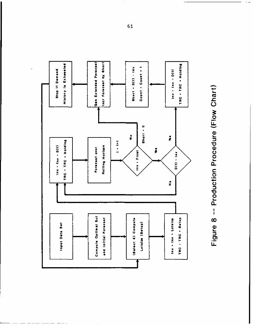
Figure 8 provides a flowchart depicting the logic of

the lot size procedure employed.

Program Validation

Verification of the computer model was obtained through

hand calculations and analysis of the results. (Discussed

in a separate section.)

61

C 0

o-

00(D

300

300

LL0 j C,0

.... . ... ... .....

62

The optimal Wagner-Whitten procedure and all lot size

heuristics were validated by hand using a data set from the

first group. The forecast model used for hand verification

of the heuristics was simple exponential smoothing with an

alpha parameter of 0.2. The code used for the

Wagner-Whitten procedures was an equivalent branch and

bound algorithm published by Jacobs and Khumawala (1987).

Verification of the code was accomplished by comparing the

results with solutions obtained using the Wagner-Whitten

algorithm by hand.

The forecast procedure was also validated by hand,

however, the overall focus forecasting policy was not.

Instead, we validated the model during program development

by comparing the focus MAD with each individual MAD for

several data sets. The focus forecast compared very

favorably, i.e., while not the best, it was significantly

better than most.

Verification of the general lot size procedure was also

obtained by hand. Specifically, the heuristics were run

using the example forecast and the results for each

transaction printed out for verification. The policy was

then computed by hand and compared with the printout.

EXPERIMENTAL DESIGN

The experimental designs for each group of data was

different due to the limited number of data sets available

in the second group.

63

The first group uses an unbalanced 5 factor design with

5 performance criteria (3 of which are the costs outlined

previously; the other 2 are measurements involving the mean

absolute deviation of the forecast series). The design is

unbalanced since 3 of the 5 factors, data set, data type,

and degree of variation, are attributes associated with the

data set. (By data set, we mean the specific data set of

which there are 36. Data type and degree of variation are

as defined earlier in our discussion of the sample data and

are nested within data set.) The other two factors are, of

course, the lot size algorithm and TBO.

The TBO factor was set at 5 levels: 2, 4, 6, 8, and 10.

To do this, we set the TBO level a-priori and determined

the appropriate A/h ratio based upon the mean or average

demand of each data set. Our procedure is therefore

similar to the studies performed by Berry (1972), Callarman

and Hamrin (1979), Wemmerl6v and Whybark (1984), and

others.

All interactions are considered except the 5-way

interaction (as it's equivalent to the error term). The

second group was handled slightly differently in that only

the primary factors, lot size algorithm and TBO, are used

in the ANOVA, i.e., we employ a simple 3-factor balanced

design with interaction.

64

RESULTS

The results for both data groups are very similar,

however the 3 factor design for the second group wasn't

able to discriminate as well as the 5 factor unbalanced

design of the first. The ANOVA results are presented in

Table 3.

I Significance IVariable I Group 1 I Group 2 I

Cost 0.001 0.001

Short 0.001 0.001

% Short 0.001 0.006

Table 3. Basic ANOVA

As you can see, both ANOVAs are significant. Tables 4

and 5 provide a "breakdown" of the significance for each

factor combination for Groups 1 and 2, respectively. The

asterisk denotes significance at the 0.01 level.

The 3- and 4-way interactions are generally significant

for cost although not for shortages or amounts short in the

Group 1 ANOVA. Results are similar for the 2-way

interactions in Group 2. The results for all common

factors and their interactions are generally the same for

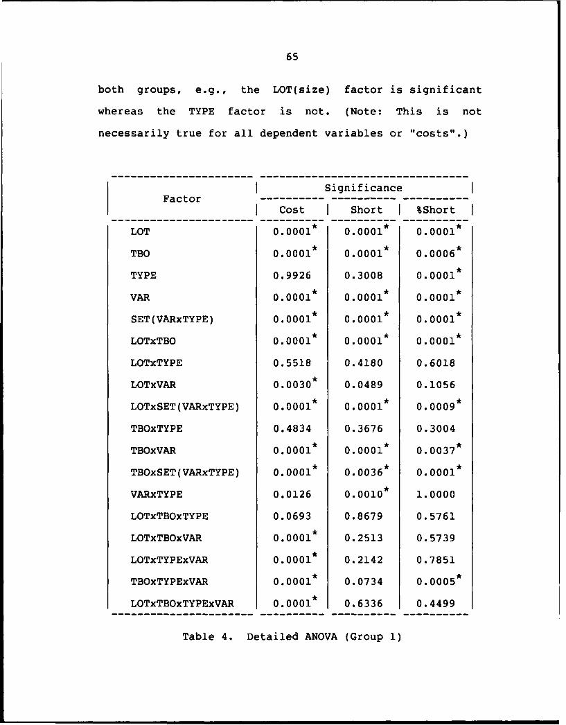
65

both groups, e.g., the LOT(size) factor is significant

whereas the TYPE factor is not. (Note: This is not

necessarily true for all dependent variables or "costs".)

I SignificanceFactor-------------- ----- ---- ----------

I Cost I Short I%ShortLOT---------- 0.0001*-- 0.0001*-- 0.0001*--

LT 0.0001* 0.0001* 0.0006*

TYPE 0.9926 0.3008 0.0001*

VAR 0.0001* 0.0001* 0.0001*

SET(VARxTYPE) 0.0001* 0.0001* 0.0001*

LOTxTBO 0.0001* 0.0001* 0.0001*

LOTxTYPE 0.5518 0.4180 0.6018

LOTxVAR 0.0030* 0.0489 0.1056

LOTxSET(VARxTYPE) 0.0001* 0.0001* 0.0009*

TBOxTYPE 0.4834 0.3676 0.3004

TBOxVAR 0.0001* 0.0001* 0.0037*

TBOxSET(VARxTYPE) 0.0001* 0.0036* 0.0001*

VARxTYPE 0.0126 0.0010* 1.0000

LOTxTBOxTYPE 0.0693 0.8679 0.5761

LOTxTBOxVAR 0.0001* 0.2513 0.5739

LOTxTYPExVAR 0.0001* 0.2142 0.7851

TBOxTYPExVAR 0.0001* 0.0734 0.0005*

LOTxTBOxTYPExVAR 0.0001* 0.6336 0.4499

Table 4. Detailed ANOVA (Group 1)

66

i SignificanceFactor I Cost I Short I %Short i

LOT 0.0001* 0.0001 0.0047

TBO 0.0001* 0.0001* 0.0180

SET 0.0124 0.3534 0.0023*

LOTxTBO 0.0001* 0.0004* 0.4349

LOTxSET 0.0001* 0.1247 0.0146

TBOxSET 0.0011* 0.2736 0.0067*

Table 5. Detailed ANOVA (Group 2)

Tables 6 and 7 give the results of the Tukey multiple

range tests for each single factor of interest.

Means with the same letters are not significantly

different and are listed from high to low. Note that the

i Factor i Cost i Short I %Short

Lotsize 51 3 24 42 3 15 42 31 5A B CCCCC AAA C AAA CCC D

BBB D BBB

TBO X 82 64 X8 6 42 X4 2 68A BBB CCC A BBBBB C AAA

BBBBBBB

Type Lin Non Lin Non Lin NonIIAAAAAAA AAAAAAAIA B

~Var 32 1 32 1 32 1A B C A B C A B C

Table 6. Single Factor Tukey Results (Group 1)

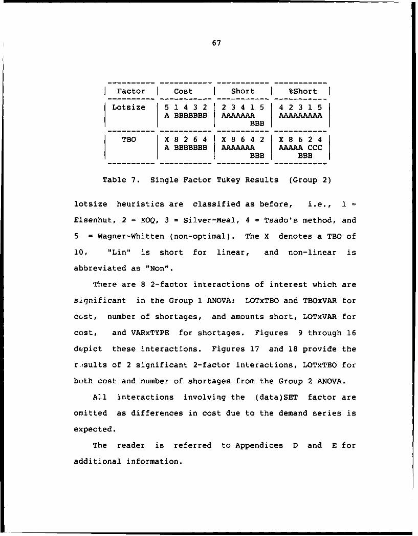
67

Factor Cost I Short i %Short I

Lotsize 5 1 4 3 2 2 3 4 1 5 4 2 3 1 5A BBBBBBB AAAAAAA AAAAAAAAA

BBB

TBO X8 2 64 X 8 642 X 8 62 4A BBBBBBB AAAAAAA AAAAA CCC

BBB BBB

Table 7. Single Factor Tukey Results (Group 2)

lotsize heuristics are classified as before, i.e., 1 =

Eisenhut, 2 = EOQ, 3 = Silver-Meal, 4 = Tsado's method, and

5 = Wagner-Whitten (non-optimal). The X denotes a TBO of

10, "Lin" is short for linear, and non-linear is

abbreviated as "Non".

There are 8 2-factor interactions of interest which are

significant in the Group 1 ANOVA: LOTxTBO and TBOxVAR for

cost, number of shortages, and amounts short, LOTxVAR for

cost, and VARxTYPE for shortages. Figures 9 through 16

depict these interactions. Figures 17 and 18 provide the

r sults of 2 significant 2-factor interactions, LOTxTBO for

both cost and number of shortages from the Group 2 ANOVA.

All interactions involving the (data)SET factor are

omitted as differences in cost due to the demand series is

expected.

The reader is referred to Appendices D and E for

additional information.

68

2-Factor Interaction (Group 1)Lotsize x TBO

Avg Inventory Costs (Holding & Setup)

350

300

250

200

150

100

50 J

Elenhut EOQ Silver-Meal Tsado W-W He

Lotaize Algorithm

TBO- 2 " 4 * 6 -8 - 10

Figure 9

69

2-Factor Interaction (Group 1)Lotslze x TBO

Ava # of Stockouts (% of Replenishments)40

356

301

15

10,>

Eisenhut EOQ Silver-Meal Teado W-W HeLotaIze Algorithm

TBO

Figure 10

70

2-Factor Interaction (Group 1)Lotsize x TBO

Avg Amount Short N% of Actual Demand)

101

40~

30

20-

110i'

1"

Eisenhut EOQ Slver-Meal Teado W-W HeLoteize Algorithm

TBO

Figure 11

71

2-Factor Interaction (Group 1)Lotaize x Variance

Avg Inventory Costs (Holding & Setup)140

120

100

Eieenhut EOQ Silver-Meal Teado W-W HeLotalze Algorithm

Variance

Low Medium High

Figure 12

72

2-Factor Interaction (Group 1)TBO x Variance

Avg Inventory Coete (Holding & Setup)1201

100!

80

....... ..-40 ' --. ... .

60 ,- 77

012 4 6 8 10

Time Between Orders (Average)

Variance

Low Medium High

Figure 13

72

2-Factor Interaction (Group 1)TBO x Variance

Avg Inventory Coete (Holding 8 Setup)120[__

100,

801801. -. " .A.""-r

60O

4 0- -------

20!01

2 4 6 a 10

Time Between Orders (Average)

Variance

-- Low - Medium High

Figure 13

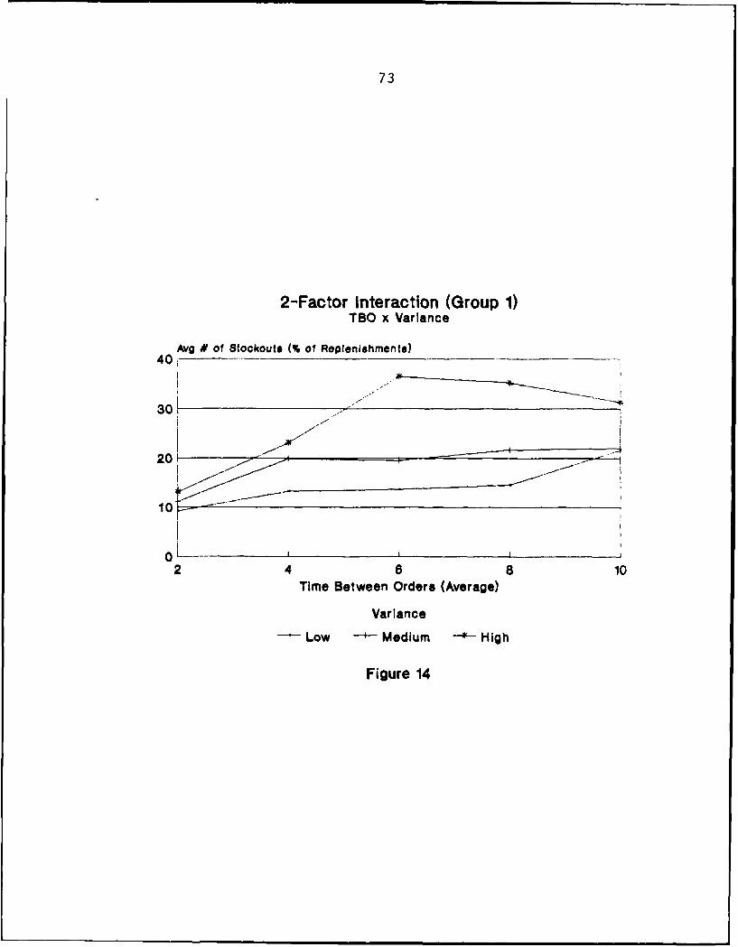
73

2-Factor Interaction (Group 1)TBO x Variance

Avg S of Stockouts (% of Replenishments)40i

30 -

10

2 4 6 8 10

Time Between Orders (Average)

Variance

Low Medium High

Figure 14

74

2-Factor Interaction (Group 1)TBO x Variance

Avg Amount Short (% of Actual Demand)60

60

40

3 0 ..

20 1 ____-

10!101

2 4 6 8 10Time Between Orders (Average)

Variance

Low g Medium High

Figure 15

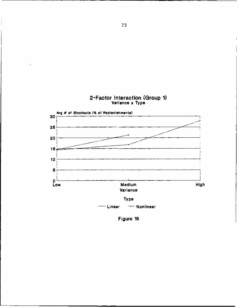
75

2-Factor Interaction (Group 1)Variance x Type

Avg # of Stookouts (% of Replenishmente)30

26

20 _

10!

6*

01Low Medium High

Variance

Type

Linear - Nonlinear

Figure 16

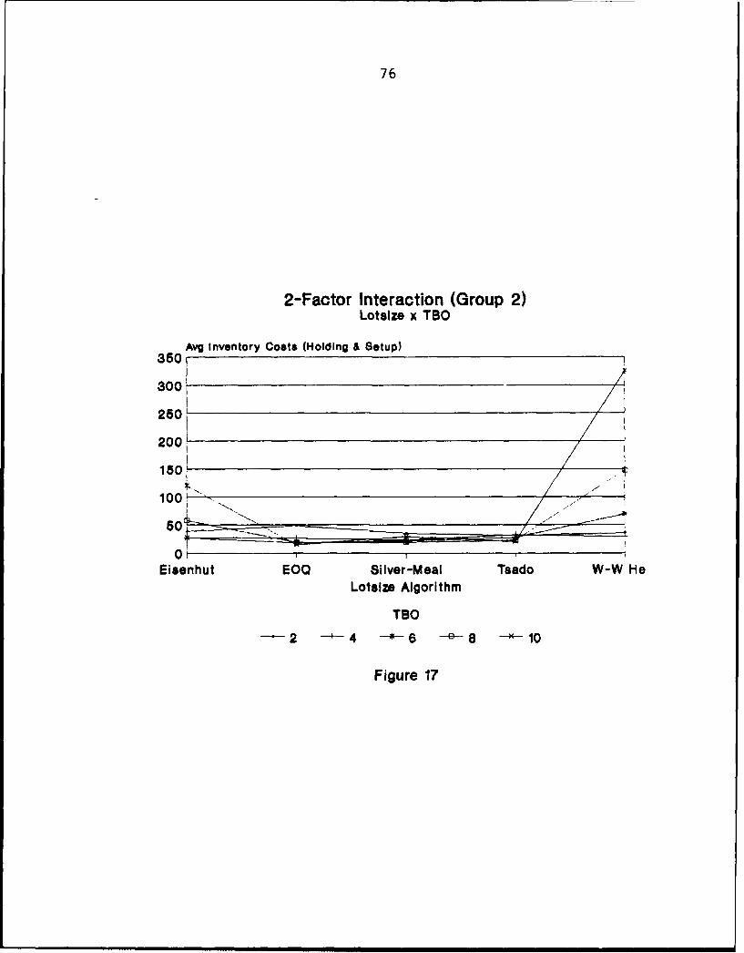
76

2-Factor Interaction (Group 2)Loteize x TBO

Avg Inventory Costs (Holding & Setup)350 - _ _ _ _ _ _ _ _ _ _ _ _ _ _ _ _ _ _ _ _ _ _ _ _ _ _

300

250

Eisenhut EOQ Silver-Meal Tsado W-W HeLoteize Algorithm

TBO-2 ~4 * 6 8 0

Figure 17

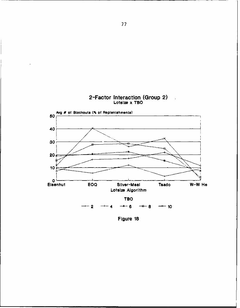
77

2-Factor Interaction (Group 2)Loteize x TBO

Avg # of $tockouts M% of Replenishments)50

40ri

20

10

01Elsenhut EOQ Silver-Meal Teado W-W He

Lotaize Algorithm

TBO

Figure 18

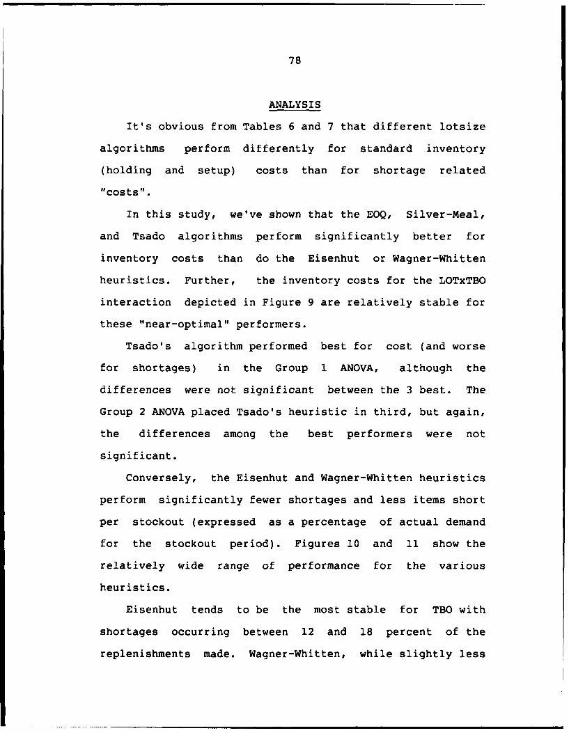
78

ANALYSIS

It's obvious from Tables 6 and 7 that different lotsize

algorithms perform differently for standard inventory

(holding and setup) costs than for shortage related

"costs".

In this study, we've shown that the EOQ, Silver-Meal,

and Tsado algorithms perform significantly better for

inventory costs than do the Eisenhut or Wagner-Whitten

heuristics. Further, the inventory costs for the LOTxTBO

interaction depicted in Figure 9 are relatively stable for

these "near-optimal" performers.

Tsado's algorithm performed best for cost (and worse

for shortages) in the Group 1 ANOVA, although the

differences were not significant between the 3 best. The

Group 2 ANOVA placed Tsado's heuristic in third, but again,

the differences among the best performers were not

significant.

Conversely, the Eisenhut and Wagner-Whitten heuristics

perform significantly fewer shortages and less items short

per stockout (expressed as a percentage of actual demand

for the stockout period). Figures 10 and 11 show the

relatively wide range of performance for the various

heuristics.

Eisenhut tends to be the most stable for TBO with

shortages occurring between 12 and 18 percent of the

replenishments made. Wagner-Whitten, while slightly less

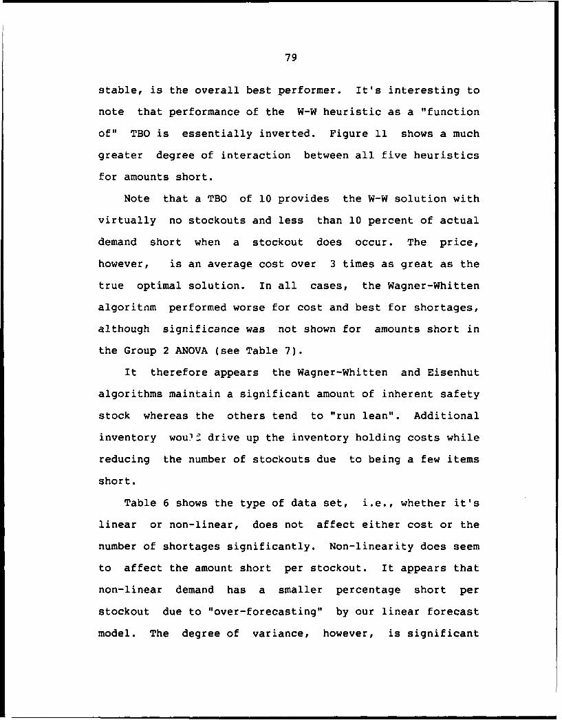
79

stable, is the overall best performer. It's interesting to

note that performance of the W-W heuristic as a "function

of" TBO is essentially inverted. Figure 11 shows a much

greater degree of interaction between all five heuristics

for amounts short.

Note that a TBO of 10 provides the W-W solution with

virtually no stockouts and less than 10 percent of actual

demand short when a stockout does occur. The price,

however, is an average cost over 3 times as great as the

true optimal solution. In all cases, the Wagner-Whitten

algoritnm performed worse for cost and best for shortages,

although significance was not shown for amounts short in

the Group 2 ANOVA (see Table 7).

It therefore appears the Wagner-Whitten and Eisenhut

algorithms maintain a significant amount of inherent safety

stock whereas the others tend to "run lean". Additional

inventory wou'f drive up the inventory holding costs while

reducing the number of stockouts due to being a few items

short.

Table 6 shows the type of data set, i.e., whether it's

linear or non-linear, does not affect either cost or the

number of shortages significantly. Non-linearity does seem

to affect the amount short per stockout. It appears that

non-linear demand has a smaller percentage short per

stockout due to "over-forecasting" by our linear forecast

model. The degree of variance, however, is significant

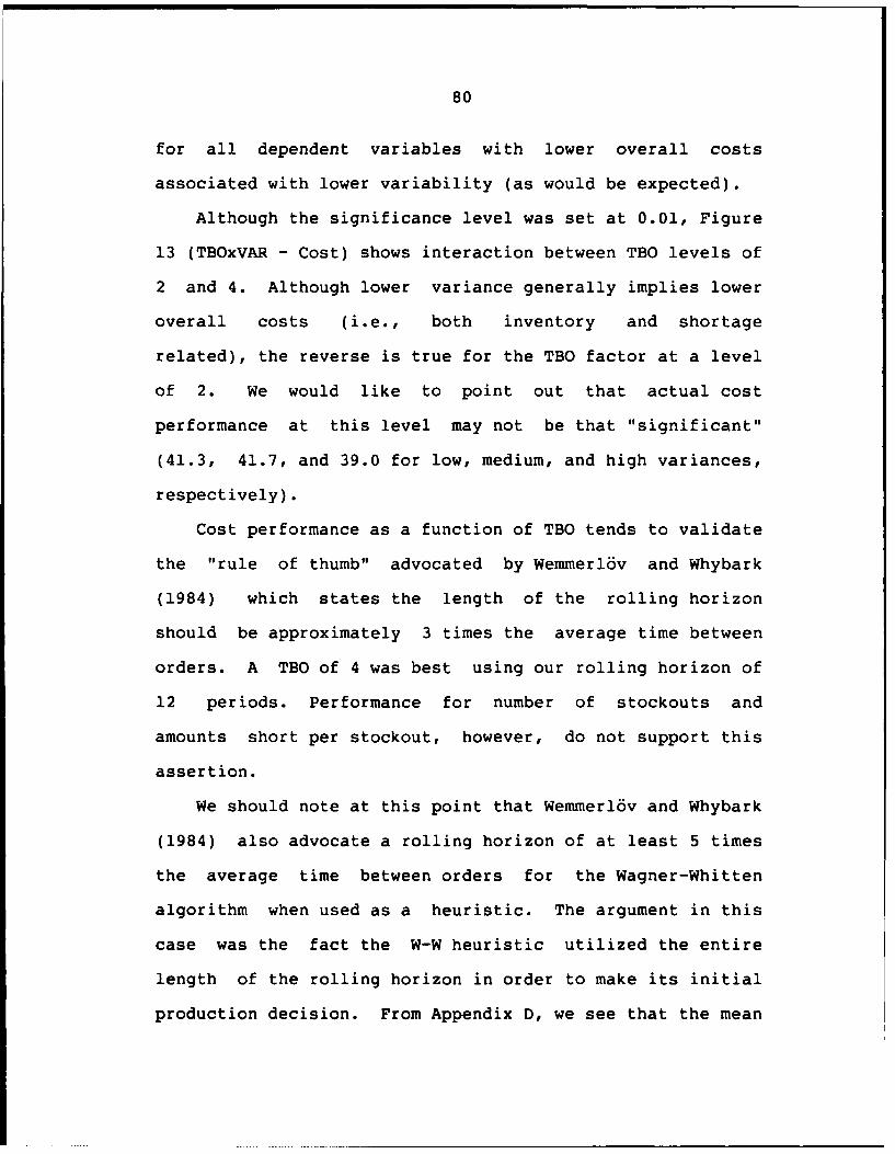
80

for all dependent variables with lower overall costs

associated with lower variability (as would be expected).

Although the significance level was set at 0.01, Figure

13 (TBOxVAR - Cost) shows interaction between TBO levels of

2 and 4. Although lower variance generally implies lower

overall costs (i.e., both inventory and shortage

related), the reverse is true for the TBO factor at a level

of 2. We would like to point out that actual cost

performance at this level may not be that "significant"

(41.3, 41.7, and 39.0 for low, medium, and high variances,

respectively).

Cost performance as a function of TBO tends to validate

the "rule of thumb" advocated by Wemmerl6v and Whybark

(1984) which states the length of the rolling horizon

should be approximately 3 times the average time between

orders. A TBO of 4 was best using our rolling horizon of

12 periods. Performance for number of stockouts and

amounts short per stockout, however, do not support this

assertion.

We should note at this point that Wemmerl6v and Whybark

(1984) also advocate a rolling horizon of at least 5 times

the average time between orders for the Wagner-Whitten

algorithm when used as a heuristic. The argument in this

case was the fact the W-W heuristic utilized the entire

length of the rolling horizon in order to make its initial

production decision. From Appendix D, we see that the mean

81

cost performance for the W-W heuristic for a TBO of 2 is

41.015926 and for a TBO of 4 is 32.546886. This tends to

discredit their assertion.

There may be 2 reasons for this. First, previous cost

criteria "consisted" of standard inventory costs and an

"artificial" service level. The mean "cost" performance

for stockouts is better for the Wagner-Whitten heuristic

with a TBO of 2 than a TBO of 4 (9.1463710 and 14.3588956,

respectively), therefore the "total costs" due to inventory

and stockouts may "average" out. (Note there was no real

difference in the amounts short for either case.) Second,

forecasts generally tend to "worsen" as they extend further

into the future. This would tend to imply that using

increasingly "bad" data in order to make the initial

production decision results in a "worse" decision.

The cost results for the TBO factor (where a TBO which

is one-third of our rolling horizon is "optimal") tend to

validate the production procedure and the computer code in

general.

Other results which tend to validate this research are

as follows:

1. The difference between all heuristic costs and

the optimal cost are strictly positive.

2. The average difference between the mean absolute

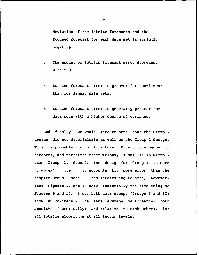
82

deviation of the lotsize forecasts and the

focused forecast for each data set is strictly

positive.

3. The amount of lotsize forecast error decreases

with TBO.

4. Lotsize forecast error is greater for non-linear

than for linear data sets.

5. Lotsize forecast error is generally greater for

data sets with a higher degree of variance.

And finally, we would like to note that the Group 2

design did not discriminate as well as the Group 1 design.

This is probably due to 2 factors. First, the number of

datasets, and therefore observations, is smaller in Group 2

than Group 1. Second, the design for Group 1 is more

"complex", i.e., it accounts for more error than the

simpler Group 2 model. It's interesting to note, however,

that Figures 17 and 18 show essentially the same thing as

Figures 9 and 10, i.e., both data groups (Groups I and II)

show alcoximately the same average performance, both

absolute (numerically) and relative (to each other), for

all lotsize algorithms at all factor levels.

CHAPTER VI

CONCLUDING REMARKS

The purpose of this research was three-fold. First,

there existed a need to perform a study of lotsize

heuristic performance which forecasts empirical demand data

in the same manner in which the lotsize heuristics are

implemented, i.e., over a rolling horizon. Second, we

wished to analyze shortage costs separately from

traditional inventory costs. And finally, we wished to

validate the heuristic presented by Tsado (1985).

The lack of significance for the LOTxVAR interaction

validates the assertion of previous studies that, although

higher variance increases costs, it doesn't alter the

relative performance of the lot size heuristics.

We have shown, however, that results from previous

studies were confounded due to the way shortage costs were

handled, i.e., by setting an arbitrary service level.

Whereas previous studies showed no significant difference

in lot size heuristic performance, we have shown that some

83

84

lot size heuristics perform better for traditional

inventory costs and others perform better with regard to

the average number of stockouts expressed as a percentage

of the total number of replenishments made and average

amounts short as a percentage of actual demand for the

stockout period.

Whether this result has any application to the way

lotsize heuristics are chosen and implemented or not is for

industry to decide. (Specifically, a company will probably

set a service level based upon its own perception

of the "cost" associated with a shortage.) However, we

believe this result is important in that it shows that

researchers should carefully choose their basic

assumptions. In this case, previous researchers would have

obtained results similar to this research if they had set

service level as a factor in their experimental designs.

But by setting a single service level, they "confounded"

the relative performance of the various lot size heuristics

examined.

And finally, we've shown that Tsado's algorithm

performed very well for traditional inventory holding and

setup costs and have therefore validated his 1985 study.

This study was by no means all-encompassing. The

following are suggestions for further research:

85

1. A similar study is required using a balanced

experimental design similar to that used by

Group 1 and using a more complete array of

lotsize techniques.

2. Separate research regarding the relative merit

of focus or "adaptive" and averaged exponential

smoothing techniques (as used in automatic

forecasting over a rolling horizon) is warranted.

REFERENCES

Amar, Amar Dev and Gupta, Jatinder N. D. (1986). Simulatedversus real life data in testing the efficiency of

scheduling algorithms. III Transactions, 18, 16-25.

Aucamp, D. C. (1985). A variable demand lot-sizingprocedure and a comparison with various well known

strategies. Production and Inventory Management, 26,2, 1-18.

Baker, K. R. and Peterson, D. W. (1979). An analyticframework for evaluating rolling schedules. Management

Sciences, 25, 341-351.

Benton, W. C. and Whybark, D. C. (1982). Materialrequirements planning (MRP) and purchase discounts.

Journal of Operations Management, 2, 137.

Barron, M. and Targett, D. (1985). The Manager's Guide toBusiness Forecasting. Oxford: Basil Blackwell Ltd.

Berry, W. L. (1972). Lot sizing procedures forrequirements planning systems: A framework for

analysis. Production and Inventory Managment, 13, 2,19-34.

Blackburn, J. D. and Millen, R. A. (1979). Selectin alot-sizing technique for a singl--level assembly

process: Part II. Empirical results. Production andInventory Management, 20, 4, 40-52.

Bookbinder, James H. and H'ng, Bak-Tee (1986). Rollinghorizon production planning for probabilistic time-

varying demands. International Journal of ProductionResearch, 24, 6, 1439-1458.

86

87

Bookbinder, James H. and Tan, Jin-Yan (1988). Strategiesfor the probabilistic lot-sizing problem with

servicelevel constraints. Management Science, 34,9, 1096-1108.

Callarman, T. E. (1979). Lot sizing for materialrequirements planning with demand uncertainty and

stockout costs as a criterion. Proceedings of the 10thAnnual Midwest AIDS Conference. New Orleans.

Callarman, T. E. and Hamrin, R. S. (1979). Lot sizingtechniques in material requirements planning with

demand uncertainty. Proceedings of the iCth AnnualMidwest AIDS Conference. Chicago.

Callarman, T. E. and Hamrin, R. S. (1984). A comparison ofdynamic lot-sizing rules for use in a single stage MRP

with demand uncertainty. International Journal ofOperations and Productions Management, 4, 39-48.

Chalmet, De Bodt, M. A. and Van Wassenhove, L. N. (1985).The effects of engineering changes and demand

uncertainty in MRP lot-sizing: A case study.International Journal of Productions Research, 23,

233-251.

De Bodt, M. A. (1983). Influence of demand uncertainty onlot-sizing and buffering decisions. Unpubli:hed

dissertation. Leuven, Belgium: Katholieke Universiteit.

De Bodt, M. A. and Van Wassenhove, L. N. (1981).Experimental and analytic evaluation of cost increases

due to demand uncertainty in MRP lot sizing with andwithout buffering. Working Paper 81-18. Leuven,

Belgium: Katholieke Universiteit.

De Bodt, M. A. and Van Wassenhove, L. N. (1983a). Lotsizes and safety stocks in MRP:A case study.

Production and Inventory Management, 24, 1, 1-16.

De Bodt, M. A. and Van Wassenhove, L. N. (1983b). Costincreases due to demand uncertainty in MRP lot sizing.

Decision Sciences, 14, 3, 345-362.

De Matteis, J. J. and Mendoza, A. G. (1968). An economiclot-sizing technique: I. The part-period algorithm.

IBM Systems Journal, 7, 30-48.

Ekern, S. (1981). Adaptive exponential smoothingrevisited. Journal of the Operational Research

Society, 32, 9, 775-782.

88

Evans, J. R. (1985). An efficient implementation of theWagner-Whitten algorithm for dynamic lot sizing.

Journal of Operations Management, 5, 229-235.

Flores, B. E. and Whybark, D. C. (1986). A comparison offocus forecasting with averaging and exponential

smoothing. Production and Inventory Management, 27, 3,96-103.

Flowers, A. D. (1980). A simulation study of smoothingconstant limits for an adaptive forecasting system.

Journal of Operations Management, 1, 2, 85-94.

Gardner, E. S. and Dannenbring, D. G. (1980). Forecastingwith exponential smoothing: some guidelines for modelselection. Decision Sciences, 11, 2, 370-383.

Groff, G. K. (1979). A lot sizing rule for time-phasedcomponent demand. Production and Inventory

Management, 20, 1, 47-53.

Heemsbergen, B. L. (1987). The part-period algorithm andleast-total-cost heuristics in single-level

discrete-demand lot sizing. Production and InventoryManagement, 28, 1, 1-19.

Hoel, P. G., Port, S. C., and Stone, C. J. (1972).Introduction to Stochastic Processes. Prospect

Heights, IL: Waveland Press, Inc.

Hofer, C. W. (1977). Conceptual constructs for formulatingcorporate and business strategy. Dover,

Massachusetts: Case Teachers Association.

Jacobs, Robert F. and Khumawala, Basheer M. (1987). Asimplified procedure for optimal single-level

lot-sizing. Production and Inventory Management, 28,3, 39-43.

Johnson, Lynwood A. and Montgomery, Douglas C. (1976).Forecasting and Time Series Analysis. New York:

McGraw-Hill Book Co.

Jenkins, G. M. (1979). Practical Experiences withModelling and Forecasting Time Series. New York:

Macmillan Publishing Co., Inc.

Lundin, R. A. and Morton, T. E. (1975). Planning horizonsfor the dynamic lot size model: Zabel vs. protective

procedures and computational results. OperationsResearch, 23, 711.

89

Makridakis, S., Andersen, A., Carbone, R., Fildes, R.,Hibon, M., Lewandowski, R., Newton, J., Parzen, E.,

and Winkler, R. (1982). The accuracy of extrapolation(time series) methods: Results of a forecasting

competition. Journal of Forecasting, 1, 111-153.

Makridakis, S., Spyros, and Winkler, R. L. (1983). Averagesof forecasts: Some empirical results. ManagementScience, 29, 9.

McLaren, B. J. (1977). A study of multiple level lotsizing procedures for management requirements planning

systems. Unpublished Dissertation. Indiana: PurdueUniversity.

Raiffa, H. (1968). Decision Analysis: IntroductoryLectures on Choices under Uncertainty. New York:

Newbery Award Records, Inc.

Ritchie, E. (1986). Lot-sizing for non-stationary demand.European Journal of Operational Research, 27, 267-273.

Ritchie, E. and Tsado, A. (1986). A review of lot-sizingtechniques for deterministic time-varying demand.

Production and Inventory Management, 27, 3, 65-79.

Saunders, G. (1987). How to use a microcomputer simulationto determine order quantity. Production and Inventory

Management Journal, 4th Qtr, 20-23.

Saydam, C. and McKnew, M. (1987). A fast microcomputerprogram for ordering using the Wagner-Whitten

algorithm. Production and Inventory Management, 28, 4,15-19.

Silver, E. A. (1981). Inventory management: A review andcritique. Operations Research, 29, 628-645.

Silver, E. A. and Meal, H. C. (1973). A heuristic forselecting lot size quantities for the case of a

deterministic time-varying demand and discreteopportunities for replenishment. Production and

Inventory Management, 14, 2, 64-74.

Silver, E. A. and Peterson, R. (1985). Decision Systemsfor Inventory Management and Production Planning, (2nd

ed.). New York: John Wiley and Sons.

Tsado, A. K. (1985a). Evaluation of the performance oflot-size techniques on deterministic and stochastic

demand. Unpublished Dissertation. England: Universityof Lancaster.

90

Tsado, A. K. (1985b). A simple inventory replenishmentpolicy for demand with uncertainty. Journal of theOperational Research Society, 36, 11.

Wagner, H. J. (1980). Research portfolio for inventorymanagement and production planning systems. OperationsResearch, 28, 445-485.

Wagner, H. J. and Whitten, T. M. (1958). Dynamic versionof the economic lot size model. Management Science,5, 1, 89-96.

Wemmerl6v, U. (1981). The ubiquitous EOQ--its relation todiscrete lot-sizing heuristics. International Journal

of Operations and Production Management, 1.

Wemmerl6v, U. (1982). A comparison of discrete,single-stage lot-sizing heuristics with special

emphasis on rules based on the marginal cost principle.Engineering Costs and Production Economics, 7, 1, 45-53.

Wemmerl6v, U. (1983). The part-period balancing algorithmand its look ahead-look back features: A theoretical

and experimental analysis of a single-stage lot-sizingprocedure. Journal of Operations

Management, 4, 1, 23-39.

Wemmerl6v, U. and Whybark, D. C. (1984). Lot-sizing underuncertainty in a rolling schedule environment.International Journal of Production Research, 22, 3,

467-484.

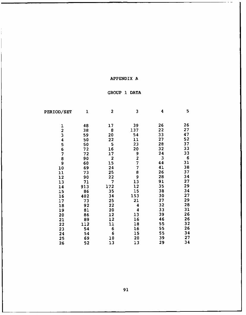
APPENDIX A

GROUP 1 DATA

PERIOD/SET 1 2 3 4 5

1 48 17 39 26 262 38 8 137 22 273 59 20 54 33 474 50 22 11 27 525 50 5 23 28 376 72 16 20 32 337 72 17 9 24 33

8 90 2 2 3 69 60 15 7 44 31

10 69 24 7 41 3811 73 25 8 26 3712 90 22 9 28 3413 71 7 13 91 2714 913 172 12 35 2915 86 35 15 38 3416 402 34 153 30 2717 73 25 21 27 2918 92 22 4 32 2819 81 20 4 33 3120 86 12 13 39 2621 89 12 16 46 2622 112 11 18 55 3223 54 6 16 55 2624 54 6 15 55 3425 69 10 20 39 2726 52 13 13 29 34

91

92

PERIOD/SET 1 2 3 4 5

27 54 17 22 35 2028 54 13 23 36 3929 39 2 13 28 3430 48 10 18 35 2731 27 8 16 25 2432 58 14 195 36 3133 32 8 335 27 2934 47 10 37 27 1635 48 14 15 27 2636 56 25 5 28 1937 67 18 18 25 4938 87 21 13 38 3639 58 21 23 31 3240 58 21 21 18 2241 66 20 17 90 2842 61 33 20 84 1343 73 18 15 24 1944 80 12 17 41 1545 62 10 30 23 2246 48 10 144 20 2647 68 11 14 22 2548 51 12 12 16 1949 47 14 7 17 2050 53 10 14 23 3151 49 10 29 23 2152 51 9 61 40 42

93

PERIOD/SET 6 7 8 9 10

1 22 26 103 35 642 16 26 77 37 523 21 44 81 35 644 14 43 67 48 805 23 47 96 54 696 22 33 83 43 557 12 39 86 57 568 3 9 12 2 159 31 19 189 154 80

10 23 31 107 60 7011 23 15 86 49 7012 31 30 100 37 6413 27 20 165 118 6614 34 25 157 48 6615 23 30 130 88 9216 21 22 238 187 8417 21 33 126 75 6318 23 36 81 42 8219 38 33 104 59 8320 21 27 94 52 8521 24 27 129 53 8922 20 23 103 39 6723 31 18 101 45 7324 28 17 133 76 8925 25 11 219 140 8526 24 14 135 64 65

94

PERIOD/SET 6 7 8 9 10

27 18 10 130 80 8128 25 29 239 112 7729 18 21 122 100 7130 9 16 105 54 6631 13 15 87 32 6632 22 19 80 67 7633 15 11 70 74 6634 20 11 88 45 7335 32 23 96 50 7436 29 30 180 116 6337 26 24 139 100 7338 26 29 126 78 6839 21 28 89 10 7340 17 17 93 52 6041 19 28 231 141 4942 15 40 123 73 4943 17 23 128 36 5044 12 33 60 41 4845 21 31 85 57 5446 15 31 73 36 5247 11 23 6i 42 5648 14 23 71 36 4149 15 26 58 20 3650 17 26 81 66 4851 20 22 67 39 3952 13 26 113 58 67

94

PERIOD/SET 6 7 8 9 10

27 18 10 130 80 8128 25 29 239 112 7729 18 21 122 100 7130 9 16 105 54 6631 13 15 87 32 6632 22 19 80 67 7633 15 11 70 74 6634 20 11 88 45 7335 32 23 96 50 7436 29 30 180 116 6337 26 24 139 100 7338 26 29 126 78 6839 21 28 89 10 7340 17 17 93 52 6041 19 28 231 141 4942 15 40 123 73 4943 17 23 128 36 5044 12 33 60 41 4845 21 31 85 57 5446 15 31 73 36 5247 11 23 61 42 5648 14 23 71 36 4149 15 26 58 20 3650 17 26 81 66 4851 20 22 67 39 3952 13 26 113 58 67

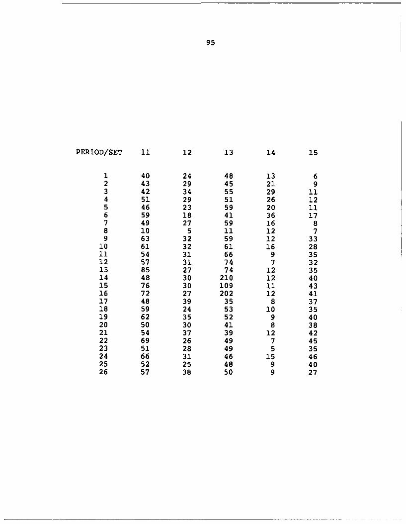
95

PERIOD/SET 11 12 13 14 15

1 40 24 48 13 62 43 29 45 21 93 42 34 55 29 114 51 29 51 26 125 46 23 59 20 116 59 18 41 36 177 49 27 59 16 88 10 5 11 12 79 63 32 59 12 33

10 61 32 61 16 2811 54 31 66 9 3512 57 31 74 7 3213 85 27 74 12 3514 48 30 210 12 4015 76 30 109 11 4316 72 27 202 12 4117 48 39 35 8 3718 59 24 53 10 3519 62 35 52 9 4020 50 30 41 8 3821 54 37 39 12 4222 69 26 49 7 4523 51 28 49 5 3524 66 31 46 15 4625 52 25 48 9 4026 57 38 50 9 27

96

PERIOD/SET 11 12 13 14 15

27 59 2 58 7 3628 73 60 65 12 3429 46 41 62 9 2930 68 35 82 11 4631 48 35 139 13 3032 52 39 162 10 4233 51 35 84 11 2534 58 31 58 9 3535 49 39 63 6 3736 47 42 36 6 2437 52 35 75 20 5038 62 42 97 15 4339 66 38 62 10 4040 35 42 102 10 2541 45 30 41 15 2242 49 37 56 14 1443 35 30 46 15 1444 40 29 50 9 1045 34 63 62 11 1046 56 79 51 15 1347 36 21 47 14 1448 29 28 57 12 1449 32 28 56 13 750 32 39 69 9 1751 36 32 69 14 1252 65 54 135 21 19

97

PERIOD/SET 16 17 18 19 20

1 51 22 10 38 32 47 6 12 21 163 41 19 23 88 184 45 50 6 57 135 29 29 54 82 226 56 32 7 52 87 55 40 33 60 228 8 3 3 9 49 32 29 12 68 15

10 42 33 9 67 2511 40 33 10 65 4812 48 36 12 61 3813 39 34 14 44 22814 56 38 10 74 6515 38 154 12 59 9316 15 49 9 43 6817 39 56 17 48 7318 42 42 28 41 8019 38 51 26 49 4820 53 22 19 64 6621 36 30 11 60 5122 46 32 27 51 11323 61 27 24 32 8624 45 23 26 38 6625 38 63 5 38 7626 35 27 13 34 59

98

PERIOD/SET 16 17 18 19 20

27 26 22 9 36 21728 50 21 26 44 7429 47 17 18 36 11830 49 28 10 45 11331 13 22 9 60 5532 184 384 22 38 10733 61 23 6 38 9034 56 12 20 32 9635 43 13 9 18 9036 50 11 19 53 10437 29 14 10 56 5738 69 29 7 61 10739 32 23 11 52 3540 35 15 42 36 2641 44 10 21 38 2842 60 47 17 42 2043 41 11 4 41 2244 54 11 16 56 1545 63 26 7 33 3046 56 5 13 48 2747 45 28 8 41 1048 41 17 15 27 2649 50 12 12 36 1050 45 22 9 40 1251 49 10 10 47 40952 100 31 9 38 21

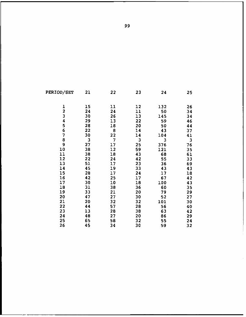
99

PERIOD/SET 21 22 23 24 25

1 15 11 12 132 262 24 24 11 50 343 30 26 13 145 344 29 13 22 59 465 28 18 20 50 446 22 8 14 43 377 30 22 14 104 418 3 7 3 3 39 27 17 25 376 7610 38 12 59 121 3511 38 18 43 68 6112 22 24 42 55 3313 51 17 23 36 6914 45 19 33 43 4315 28 17 24 17 1816 42 25 17 67 4217 30 10 18 100 4318 31 38 36 60 3519 33 21 20 79 2920 47 27 30 52 2721 20 32 32 101 3022 44 57 28 56 4023 13 28 38 63 4224 48 27 20 86 2925 65 58 32 55 2426 45 34 30 59 32

100

PERIOD/SET 21 22 23 24 25

27 62 42 31 65 2328 62 33 21 29 3429 78 29 33 129 3930 58 113 29 47 3231 76 39 33 47 3132 62 41 32 57 3833 66 46 38 72 2734 84 52 48 52 4335 77 37 27 99 2736 72 87 42 84 4137 43 44 19 51 3938 50 45 39 74 3039 39 35 37 49 3940 46 28 22 44 3241 42 35 14 35 2442 44 32 14 60 3943 32 21 12 31 2744 50 18 12 66 3145 22 30 15 73 7746 39 25 6 56 3847 42 31 15 61 5248 28 35 6 53 2349 21 12 9 43 3350 28 16 15 46 3151 16 9 8 57 1652 24 20 18 82 51

101

PERIOD/SET 26 27 28 29 30

1 155 14 12 13 132 102 14 3 14 173 83 17 5 32 224 112 19 9 25 145 84 18 5 28 206 99 18 5 33 137 117 16 4 32 118 9 1 1 6 79 212 9 6 9 14

10 88 15 7 7 1411 130 10 3 12 1712 148 17 9 10 1213 209 13 4 8 1514 150 12 5 14 1515 236 16 6 11 1416 112 16 5 5 1917 147 6 5 10 2118 94 20 4 4 819 132 17 6 9 1420 97 17 9 7 1121 113 23 7 14 922 200 16 5 9 1123 117 22 8 6 924 124 17 12 10 1225 120 19 5 10 1126 56 16 8 8 11

102

PERIOD/SET 26 27 28 29 30

27 105 28 5 11 1028 99 22 3 15 229 149 10 6 8 1230 88 23 5 10 931 78 19 5 9 1132 96 19 3 3 1233 103 28 6 15 1234 102 23 8 12 1235 103 19 6 9 1536 102 30 7 11 1337 82 16 3 10 1338 165 15 4 15 1039 76 13 5 11 1540 79 14 4 11 1541 59 11 6 13 1242 108 10 5 13 1243 88 13 8 11 2244 85 9 8 12 945 155 11 5 10 846 126 11 9 14 1647 128 18 8 11 1148 82 17 9 13 749 144 9 9 16 850 97 15 9 7 951 61 9 8 16 2352 186 26 21 21 22

103

PERIOD/SET 31 32 33 34 35

1 23 3 23 22 92 29 5 20 17 113 18 13 60 37 134 19 10 29 10 115 41 11 62 29 106 11 8 37 28 147 19 13 23 16 118 1 4 4 1 39 5 5 48 25 19

10 23 5 60 31 1411 35 8 59 33 1512 41 7 114 29 1713 40 8 56 23 714 14 6 37 21 1415 83 2 54 30 1016 32 5 42 39 617 16 8 32 17 1618 47 5 20 25 1319 22 4 48 22 1220 23 8 26 40 1121 93 6 22 16 1422 25 7 31 28 1123 22 5 15 17 924 21 5 43 17 1125 33 5 19 13 1226 23 4 46 20 17

104

PERIOD/SET 31 32 33 34 35

27 69 5 17 12 1828 82 5 20 29 1229 14 1 20 12 1430 14 8 24 15 1531 29 5 22 12 1432 23 6 48 8 733 26 8 31 12 934 18 3 24 24 1035 8 2 29 15 1136 24 1 37 22 837 28 6 25 27 1038 45 9 34 25 539 18 10 39 29 1140 39 2 57 24 441 27 4 36 14 442 20 6 42 28 743 25 7 15 14 1044 17 4 32 15 945 35 6 36 11 746 22 5 38 11 547 34 5 109 36 848 23 4 51 18 449 20 8 43 23 1150 27 3 37 19 651 36 3 18 13 752 39 9 37 36 14

105

PERIOD/SET 36

1 312 183 384 165 266 327 218 69 10

10 1911 3112 2613 2914 3615 2916 5517 1818 2419 4820 3821 1522 4923 1324 6825 1426 12

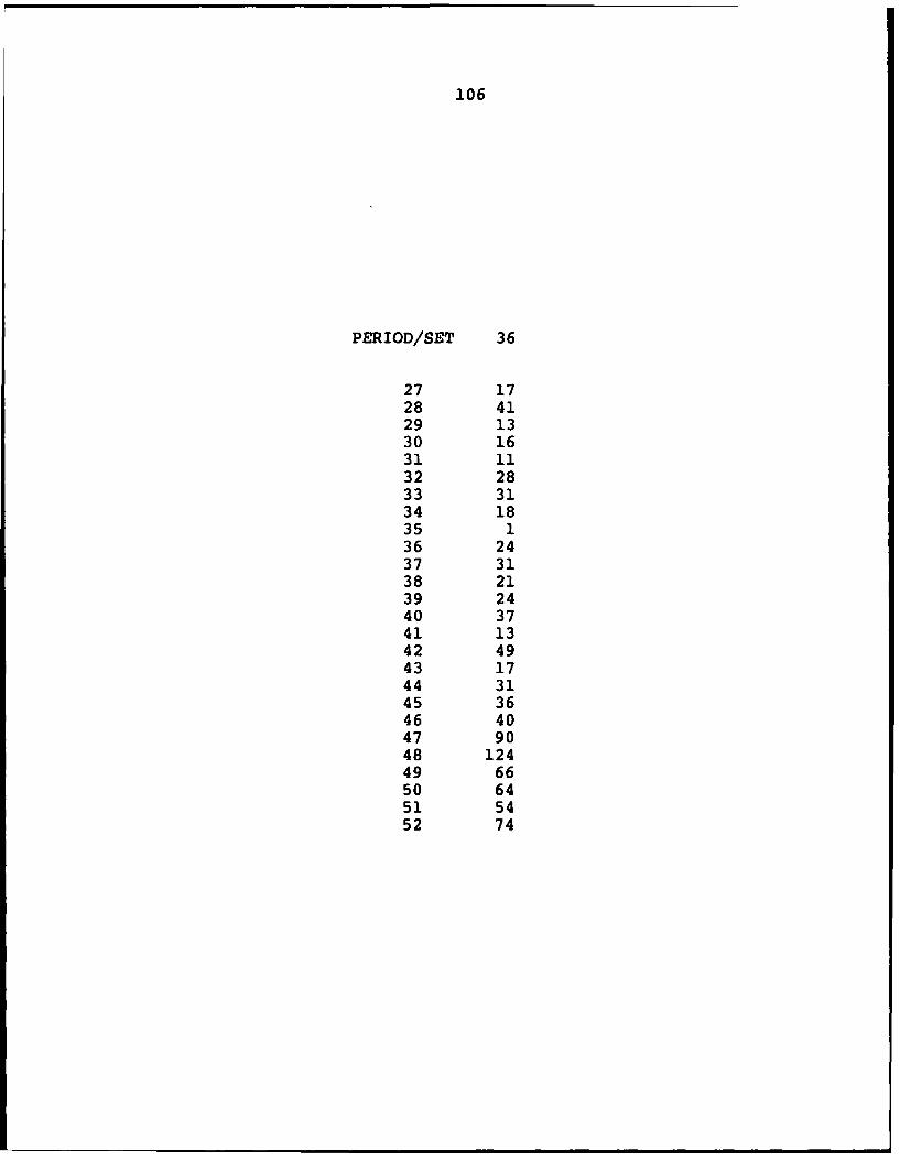
106

PERIOD/SET 36

27 1728 4129 1330 1631 1132 2833 3134 1835 136 2437 3138 2139 2440 3741 1342 4943 1744 3145 3646 4047 9048 12449 6650 6451 5452 74

APPENDIX B

GROUP 2 DATA

PERIOD/SET 1 2 3 4 5

1 1053 441 548 783 1762 1254 558 795 511 923 1566 402 993 2116 444 1659 234 1103 2998 845 1143 363 927 954 1246 1374 306 831 1299 2547 1353 189 845 1245 638 1296 114 665 1274 1419 1920 387 888 1151 147

10 1248 444 539 1316 8611 1104 327 363 804 17512 909 318 370 488 3413 945 239 425 832 13114 870 376 375 2076 4715 1247 399 451 835 15416 990 398 348 1124 6817 1422 281 461 1436 6818 1359 282 459 1267 13719 1113 227 437 2020 15020 1479 340 465 832 7321 1455 380 401 909 11322 1029 671 426 718 6523 998 562 102 646 6024 966 522 0 656 6125 627 277 1136 633 2426 723 341 821 744 64

107

108

PERIOD/SET 1 2 3 4 5

27 885 512 848 632 3628 1323 431 1231 676 2729 1137 361 928 685 10630 1389 386 867 819 7931 1455 3880 656 402 7232 1110 555 1084 519 3833 1470 1583 1302 694 6134 867 2667 1263 531 4635 1095 2626 997 486 6836 861 2584 1208 517 2637 465 1907 1353 247 2038 771 1540 1038 404 8639 756 1163 1207 330 2940 1038 908 1223 245 2241 1356 863 1002 213 4342 1521 751 1173 209 3443 1194 683 802 103 9044 1158 2231 1548 190 1545 1569 2578 2309 309 3346 957 922 882 133 2847 798 1085 1094 99 1548 686 1059 1305 168 1549 633 1162 1918 266 21450 639 973 1216 180 12051 894 749 2409 274 10852 837 971 1907 331 106

109

PERIOD/SET 1 2 3 4 5

53 918 903 1370 174 13654 987 974 1136 120 9655 1035 979 936 78 3156 840 858 1284 98 7257 1107 1105 2340 96 15658 801 1419 1444 121 10659 714 1119 1530 146 10260 696 963 1376 171 14861 570 919 1319 109 9662 357 937 1480 125 10063 525 1588 1291 201 10864 696 876 1407 127 12065 870 656 1108 110 11366 570 508 978 139 13967 657 581 1149 55 15168 750 867 776 132 9269 669 1198 1566 84 9670 474 1368 1216 180 10271 402 1104 1389 231 14872 414 1190 1719 135 19473 315 894 882 127 14574 402 883 1266 177 15375 504 887 1499 116 14776 429 906 1141 175 14477 372 833 1153 113 15778 315 697 996 158 197

APPENDIX C

PROGRAM LISTING

DECLARE SUB eoq ()DECLARE SUB tsado ()DECLARE SUB wwheuristic ()DECLARE SUB eoqtimesupply ()DECLARE SUB eisenhut ()DECLARE SUB silvermeal ()DECLARE SUB wagnerwhitten ()DECLARE SUB forecaster ()COMMON SHARED /Adata/ cost, count, datatype, holding,

horizon, inventory, k9COMMON SHARED /Bdata/ lastn, mad, n, production, setup,

sigma, xbarDEFSNG A-Zx = 10 'Dummy variable to allow dynamic dimensioning of

demand(n) and forecast(n)DIM SHARED D(x), demand(x), forecast(x, x), lotdata(x)DIM SHARED R(x), a(x, x), O(x)'Iterate through all 'DATA setsFOR dataset = 1 TO 5READ xbar, sigma, datatype, nhorizon = 12 '12 weeks (3 months) for weekly DATA or 12

months for yearly dataERASE demand, forecast, D, lotdataREDIM SHARED D(horizon), demand(n), forecast(n + 1, 2),

lotdata(n + horizon)FOR i = 1 TO n: READ demand(i): NEXT iIF n = 52 THEN lastn = 6 ELSE lastn = 12'Compute variation as Low (1), Medium (2), or High (3)IF sigma / xbar <= .5 THEN

variation = 1ELSE

IF sigma / xbar > 11 THENvariation = 3

ELSEvariation = 2

110

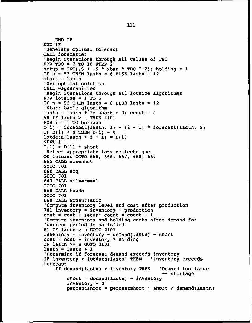
END IFEND IF'Generate optimal forecastCALL forecaster'Begin iterations through all values of TBOFOR TBO = 2 TO 10 STEP 2setup = INT(.5 + .5 * xbar * TBO ^ 2): holding = 1IF n = 52 THEN lastn = 6 ELSE lastn = 12start = lastn'Get optimal solutionCALL wagnerwhitten'Begin iterations through all lotsize algorithmsFOR lotsize = 1 TO 5IF n = 52 THEN lastn = 6 ELSE lastn = 12'Start basic algorithmlastn = lastn + 1: short = 0: count = 058 IF lastn > n THEN 2101FOR i = 1 TO horizonD(i) = forecast(lastn, 1) + (i - 1) * forecast(lastn, 2)IF D(i) < 0 THEN D(i) = 0lotdata(lastn + i - 1) = D(i)NEXT iD(l) = D(1) + short'Select appropriate lotsize techniqueON lotsize GOTO 665, 666, 667, 668, 669665 CALL eisenhutGOTO 701666 CALL eoqGOTO 701667 CALL silvermealGOTO 701668 CALL tsadoGOTO 701669 CALL wwheuristic'Compute inventory level and cost after production701 inventory = inventory + productioncost = cost + setup: count = count + 1'Compute inventory and holding costs after demand for'current period is satisfied61 IF lastn > n GOTO 2101inventory = inventory - demand(lastn) - shortcost = cost + inventory * holdingIF lastn >= n GOTO 2101lastn = lastn + 1'Determine if forecast demand exceeds inventoryIF inventory > lotdata(lastn) THEN 'Inventory exceedsforecast

IF demand(lastn) > inventory THEN 'Demand too large-- shortage

short = demand(lastn) - inventoryinventory = 0percentshort = percentshort + short / demand(lastn)

112

shortcounter = shortcounter + 1lastn = lastn + 1GOTO 58 'Setup a new production run

ELSE 'Demand was less than our inventory -- delivercurrent demand

short = 0GOTO 61 'Deliver next period's demand

END IFELSE 'Next period's forecast for demand exceeds currentinventory

short = 0GOTO 58 'Setup a new production run

END IF'Calculate the true mean absolute deviation for all periods'included in the lotsize problem2101 FOR 1 = start + 1 TO nlotsizeforecasterror = lotsizeforecasterror +ABS(lotdata(l) - demand(l))lotsizetrackingsignal = lotsizetrackingsignal + demand(l) -lotdata(l)NEXT 1lotsizeforecasterror = lotsizeforecasterror / (n - start)lotsizetrackingsignal = lotsizetrackingsignal /

(lotsizeforecasterror * (n - start))'Subtract holding costs for periods beyond N from the total'cost -- this will reduce the variability between TBOs'(treatments).cost = cost - inventory * holding'Compute PERCENTSHORT if SHORTCOUNTER is nonzero (to'prevent division by 0).IF shortcounter > 0 THEN percentshort = percentshort /shortcounter * 100'Change SHORTCOUNTER into the fraction of times short to'number of replenishments made (COUNT = (approx.) TBO --'this will reduce the variability due to TBO (e.g. a model'with a TBO of 2 can havequite a few more shortages in a'given time period than a model with a TBO of 10).shortcounter = 100 * shortcounter / count'Output results to 'DATA file in current directory.3PEN "THESIS2.OUT" FOR APPEND AS #1WRITE #1, dataset, datatype, variation, sigma / xbar, TBO,

lotsize, 100 * (cost - k9) / k9, shortcounter,percentshort, 100 * (lotsizeforecasterror - mad)/ mad, 100 * lotsizeforecasterror / xbar, 100 *lotsizetrackingsignal

CLOSE #1'Note: The 'DATA is given in percentages to provide'non-exponential format in the output (in order to allow'SAS to read the DATA directly (after the commas are'removed)).'Zero appropriate variables.inventory = 0: production = 0: lotsizeforecasterror = 0:

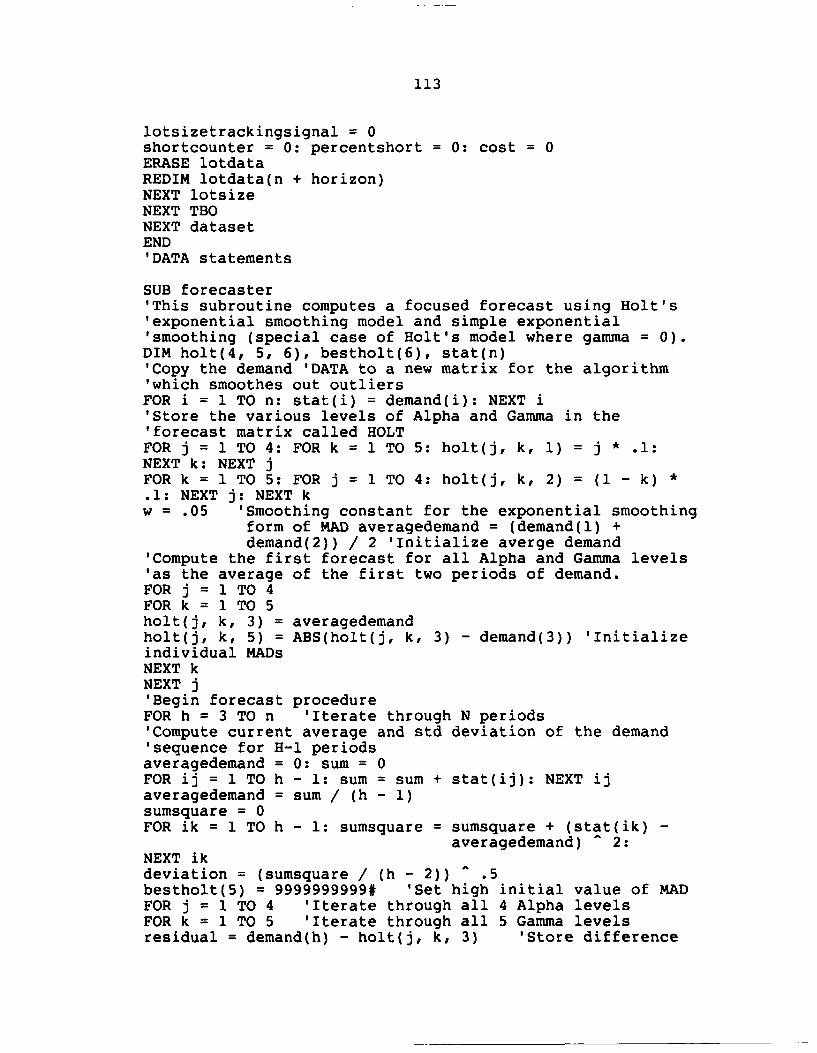
113

lotsizetrackingsignal = 0shortcounter = 0: percentshort = 0: cost = 0ERASE lotdataREDIM lotdata(n + horizon)NEXT lotsizeNEXT TBONEXT datasetEND'DATA statements

SUB forecaster'This subroutine computes a focused forecast using Holt's'exponential smoothing model and simple exponential'smoothing (special case of Holt's model where gamma = 0).DIM holt(4, 5, 6), bestholt(6), stat(n)'Copy the demand 'DATA to a new matrix for the algorithm'which smoothes out outliersFOR i = 1 TO n: stat(i) = demand(i): NEXT i'Store the various levels of Alpha and Gamma in the'forecast matrix called HOLTFOR j = 1 TO 4: FOR k = 1 TO 5: holt(j, k, 1) = j * .1:NEXT k: NEXT jFOR k = 1 TO 5: FOR j = 1 TO 4: holt(j, k, 2) = (1 - k) *.1: NEXT j: NEXT kw = .05 'Smoothing constant for the exponential smoothing

form of MAD averagedemand = (demand(l) +demand(2)) / 2 'Initialize averge demand

'Compute the first forecast for all Alpha and Gamma levels'as the average of the first two periods of demand.FOR j = 1 TO 4FOR k = 1 TO 5holt(j, k, 3) = averagedemandholt(j, k, 5) = ABS(holt(j, k, 3) - demand(3)) 'Initializeindividual MADsNEXT kNEXT j'Begin forecast procedureFOR h = 3 TO n 'Iterate through N periods'Compute current average and std deviation of the demand'sequence for H-1 periodsaveragedemand = 0: sum = 0FOR ij = 1 TO h - 1: sum = sum + stat(ij): NEXT ijaveragedemand = sum / (h - 1)sumsquare = 0FOR ik = 1 TO h - 1: sumsquare = sumsquare + (stat(ik) -

averagedemand) ^ 2:NEXT ikdeviation = (sumsquare / (h - 2)) ^ .5bestholt(5) = 9999999999# 'Set high initial value of MADFOR j = 1 TO 4 'Iterate through all 4 Alpha levelsFOR k = 1 TO 5 'Iterate through all 5 Gamma levelsresidual = demand(h) - holt(j, k, 3) 'Store difference

114

between last estimateand actual demand'Discount outliers (virtually all points should fall within'3 or 4 std deviations if the points are distributed'normally).IF datatype = 1 THEN 'Only valid for constant andslightly trending demand

IF deviation > 0 THENIF ABS(residual) / deviation > 4 THEN

residuaL = SGN(residual) * 4 * deviationstat(h) = residual + averagedemand

ELSEEND IF

ELSEEND IF

ELSEEND IFtemp = holt(j, k, 3) 'Store last estimate (the one forcurrent period'sdemand)'Compute new estimate.holt(j, k, 3) = (1 - holt(j, k, 1)) * (holt(j, k, 3) +

holt(j, k, 4)) + holt(j, k, 1) * stat(h)IF holt(j, k, 3) < 0 THEN holt(j, k, 3) = 0'Compute new trend.holt(j, k, 4) = (1 - holt(j, k, 2)) * holt(j, k, 4) +

holt(j, k, 2) * (holt(j, k, 3) - temp)'Compute current MAD and current smoothed forecast error.holt(j, k, 5) = (1 - w) * (holt(j, k, 5)) + w *ABS(residual)holt(j, k, 6) = (1 - w) * (holt(j, k, 6)) + w * residual'Determine the best forecast to date.trackingsignal = holt(j, k, 6) / holt(j, k, 5)'As defined by Silver and Peterson (1985)'Note: A negatively biased forecast (i.e.,, where forecast'exceeds demand) is preferable to a positively biased'forecast (i.e.,, where demand exceeds forecast) sincebeing'a few items overstock ("safety stock") is preferable to'consistently being a few items short (causing too many'premature setups). [See EOQ example, Ibid.]IF trackingsignal < .3 AND trackingsignal > -.9 THEN

IF holt(j, k, 5) < bestholt(5) THENbestholt(l) = holt(j, k, 1)'Alpha of best forecast for the periodbestholt(2) = holt(j, k, 2)'Gamma of best forecast for the periodbestholt(3) = holt(j, k, 3)'Best smoothed estimatebestholt(4) = holt(j, k, 4)'Best smoothed trendbestholt(5) = holt(j, k, 5)

115

'Best MAD for the periodbestholt(6) = holt(j, k, 6)'Best smoothed forecast error for the period

ELSEEND IF

ELSEEND IFNEXT k 'Next GammaNEXT j 'Next Alpha'Now store the best forecast for this period (which is the'forecast for 'demand in period H+l, i.e., the nextperiod).forecast(h + 1, 1) = INT(.5 + bestholt(3))forecast(h + 1, 2) = INT(.5 + bestholt(4))NEXT h 'Next period'Compute the MAD for the entire forecast over N - Lastn'periods.mad = 0FOR i = lastn + 1 TO n: mad = mad + ABS(forecast(i, 1) -demand(i)): NEXT imad = mad / (n - lastn)'Compute the tracking signal for the entire forecast over N'- Lastn periods.track = 0FOR i = lastn + 1 TO n: track = track + demand(i) -

forecast(i, 1): NEXT itrackingsignal = track / (mad * (n - lastn))END SUB

SUB silvermealDIM trc(24), trcut(24)trc(l) = 0: trcut(l) = 0: production = 0trc(l) = setup: trcut(l) = trc(l)FOR kk = 2 TO horizontrc(kk) = trc(kk - 1) + (kk - 1) * D(kk) * holdingtrcut(kk) = trc(kk) / kkIF trcut(kk) > trcut(kk - 1) THEN 55NEXT kk55 FOR 1 = 1 TO kk - 1production = production + D(l)NEXT 1production = production - inventoryEND SUB

SUB eisenhut 'part-period balancingDIM trc(24), trcut(24)trc(l) = 0: production = 0FOR kk = 2 TO horizontrc(kk) = trc(kk - 1) + (kk - 1) * D(kk) * holding'determine first period where accumulated holding costs'exceeds setupIF trc(kk) > setup THEN

116

'determine which integer period is closer to actual setup'costs

IF ABS(trc(kk) - setup) > ABS(trc(kk - 1) - setup)THEN

lastperiod = kk - 1ELSE

lastperiod = kkEND IFGOTO 565

ELSE 'continue to next period, i.e., next kkEND IFNEXT kk565 FOR 1 = 1 TO lastperiodproduction = production + D(l)NEXT 1production = production - inventoryEND SUB

SUB eoqproduction = 0: avg = 0FOR i = 1 TO horizonavg = avg + D(i)NEXT iavg = avg / horizonproduction (2 * avg * setup / holding) .5 + shortproduction = INT(.5 + production) - inventoryEND SUB

SUB tsadoproduction = 0: avg = 0FOR i = 1 TO horizonavg = avg + D(i)NEXT iavg = avg + short: avg = avg / horizontime = lastn - 7production = -avg * time + ((avg * time) 2 + (2 * avg *(cost + setup) /holding)) .5production = INT(.5 + production) - inventoryEND SUB

SUB wagnerwhitten5 ERASE R, a, 010 REDIM R(n), a(5000, 5), O(n)60 m = n - lastn110 FOR i = 1 TO m: R(i) = demand(i + 6): NEXT i120 S = setup130 C = holding150 a(l, 1) = 1160 a(1, 2) = 1170 a(l, 3) = S180 a(l, 4) = 0

117

190 a(l, 5) = 1200 Ni = 0210 N2 = 1220 FOR i = 1 TO m230 IF R(i) = 0 THEN 530240 k9 = 999999999#250 K8 = 0260 FOR k = 1 TO N2270 IF a(N1 + k, 3) > k9 THEN 320280 K8 = Ni + k290 k9 = a(K8, 3)300 K7 = k9 + S320 NEXT k330 N3 = 1340 j = Ni + N2350 a(j + N3, 1) = i360 a(j + N3, 2) = 1370 a(j + N3, 3) = K7380 a(j + N3, 4) = K8390 a(j + N3, 5) = i400 FOR k = 1 TO N2410 Cl = (i - a(Nl + k, 5)) * C * R(i)420 IF Cl > S THEN 500430 IF a(Nl + k, 4) + Cl > K7 THEN 540440 N3 = N3 + 1450 a(j + N3, 1) = i460 a(j + N3, 2) = 0470 a(j + N3, 3) = a(Nl + k, 3) + Cl480 a(j + N3, 4) = Ni + k490 a(j + N3, 5) = a(Nl + k, 5)500 NEXT k510 Ni = j520 N2 = N3530 NEXT i540 k9 = 999999999#550 K8 = 0560 FOR k = 1 TO N2570 IF a(N1 + k, 3) > k9 THEN 600580 K8 = Ni + k590 k9 = a(K8, 3)600 NEXT k610 'Solution Cost = k9620 IF a(K8, 2) = 0 THEN 640630 O(a(K8, 1)) = 1640 K8 = a(K8, 4)650 IF a(K8, 4) = 0 THEN 670660 GOTO 620670 FOR i = 1 TO m680 IF i = 1 THEN 720690 IF O(i) = 0 THEN 730720 Q = 0730 Q = Q + R(i)

118

740 NEXT iEND SUB

SUB wwheuristic1105 ERASE R, a, 01110 REDIM R(horizon), a(1000, 5), O(horizon)1115 production = 0: flag = 01160 m = horizon11110 FOR i = 1 TO m: R(i) = D(i): NEXT i11120 S = setup11130 C = holding11150 a(l, 1) = 111160 a(l, 2) = 111170 a(l, 3) = S11180 a(l, 4) = 011190 a(l, 5) = 111200 Ni = 011210 N2 = 111220 FOR i = 1 TO m11230 IF R(i) = 0 THEN 1153011240 k999 = 999999999#11250 K8 = 011260 FOR k = 1 TO N211270 IF a(Nl + k, 3) > k999 THEN 1132011280 K8 = Ni + k11290 k999 = a(K8, 3)11300 K7 = k999 + S11320 NEXT k11330 N3 = 111340 j = Ni + N211350 a(j + N3, 1) = i11360 a(j + N3, 2) = 111370 a(j + N3, 3) = K711380 a(j + N3, 4) = K811390 a(j + N3, 5) = i11400 FOR k = 1 TO N211410 Cl = (i - a(Nl + k, 5)) * C * R(i)11420 IF Cl > S THEN 1150011430 IF a(Nl + k, 4) + Cl > K7 THEN 1154011440 N3 = N3 + 111450 a(j + N3, 1) = i11460 a(j + N3, 2) = 011470 a(j + N3, 3) = a(Nl + k, 3) + Cl11480 a(j + N3, 4) = Ni + k11490 a(j + N3, 5) = a(Nl + k, 5)11500 NEXT k11510 Ni = j11520 N2 = N311530 NEXT i11540 k999 = 999999999#11550 K8 = 011560 FOR k = 1 TO N2

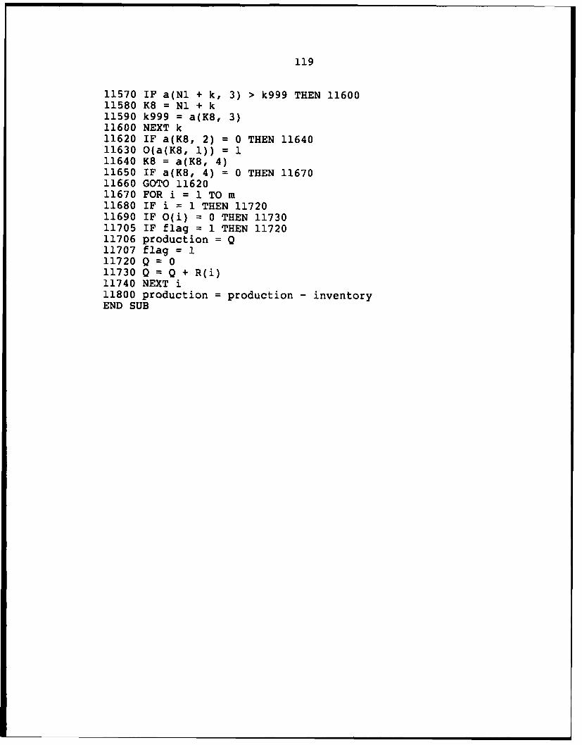
119

11570 IF a(Nl + k, 3) > k999 THEN 1160011580 K8 = Ni + k11590 k999 = a(K8, 3)11600 NEXT k11620 IF a(K8, 2) = 0 THEN 1164011630 O(a(K8, 1)) = 111640 K8 = a(K8, 4)11650 IF a(K8, 4) = 0 THEN 1167011660 GOTO 1162011670 FOR i = 1 TO m11680 IF i = 1 THEN 1172011690 IF O(i) = 0 THEN 1173011705 IF flag = 1 THEN 1172011706 production = Q11707 flag = 111720 Q = 011730 Q = Q + R(i)11740 NEXT i11800 production = production - inventoryEND SUB

APPENDIX D

ANOVA RESULTS -- GROUP I DATA

The following text provides the code used in the SAS

routine. Output consists of all subsequent pages.

DATA;INPUT SET TYPE VAR COFVAR TBO LOT COST SHORTPERSHORT DELERR PERERR BIAS;DROP COFVAR BIAS;CARDS;

PROC ANOVA;CLASS SET TBO LOT VAR TYPE;MODEL COST SHORT PERSHORT DELERR PERERR = LOT TBO

TYPE VAR SET(TYPE VAR) LOT*TBO LOT*TYPELOT*VAR LOT*SET(TYPE VAR) TBO*TYPE TBO*VARTBO*SET(TYPE VAR) TYPE*VAR LOT*TBO*TYPELOT*TBO*VAR LOT*TYPE*VAR TBO*TYPE*VARLOT*TBO*TYPE*VAR;

MEANS LOT TBO TYPE VAR LOT*TBO LOT*TYPE LOT*VARTYPE*VAR TBO*TYPE TBO*VAR LOT*TBO*TYPELOT*TBO*VAR LOT*TYPE*VAR LOT*TBO*TYPE*VAR/ TUKEY;

OUTPUT OUT=PLOTDATA P=YPRED R=YRESID;PROC UNIVARIATE NORMAL PLOT;

VAR YRESID;PROC PLOT;

PLOT YRESID*YPRED;PLOT YRESID*LOT;PLOT YRESID*TBO;

120

121

UALYS!S OF VIIUC';E PROCIED E

CLASS LEVEL IvOnATI8O

CLASS LEVELS FLUES

SET 36 1 2 3 4 5 0 1 8 9 10 11 12 13 14 15 I t ll 18 10 2.

2! 22 23 24 25 25 21 26 29 3R C 32 33 34 35 36

TBO 5 246810

LOT 5 1234 5

VAR 3 i-2 3

TME 2 0 i

iVIG OF OBSERVAT!OIS 20 DATA SE! O

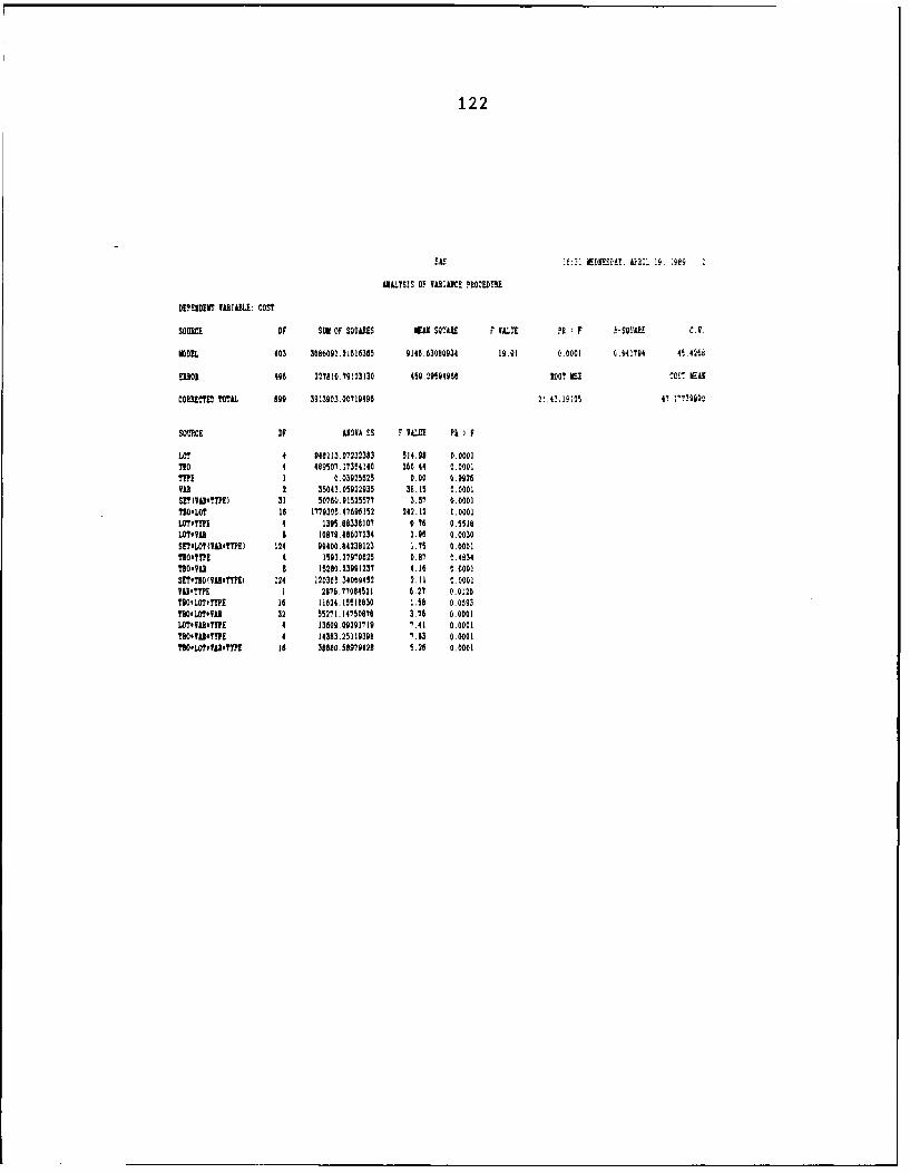
122

UALYSIS OF VLAIIC! PROCEDURE

DMIDENT VAIIABLE: COS?

SOURCE OF SUM OF SQUARES mOi SQ0L F VZUE ?I F 0-500.1 C.V

MODEL 403 36060g2.210816385 9146.63000934 19.91 0.001 C.04!794 45.426i

110 496 227810.79!03130 459.2959490 0? IE COO IEL

CORRECTED ?0?9L g9 39!3903.00719496 .!0205 47. 772903

SOURCE DF 191VA SS F VA.U H ) F

LOO 4 946113.07232393 514.90 0.0001

To 4 409507.1735440 26(.44 0.000.770E 1 0.03925825 0.00 0.9926VAR 2 35043.05922935 30.15 0.0001S"lS? I.?TPE) 31 50760.01525577 3.51 0.0001

TOLOT l 1779305.47696152 242.12 0.0001IO9?TMP1 4 1395.80338107 0.78 0.5516

LO VAI 8 10870.88607234 2.98 0.0030SETLOT(VR@RTYPEI 124 99400.84230123 1.75 0.0001710,T. t 4 1593.27970625 0.87 0.4834TbOVil 6 15290.23991237 4.16 0.0001

SETTI.(ld7 TYP[I 124 1203E5.34069452 2.11 0,00017TTP. E 1 2876.77084521 6.27 0.0126

TBO-LOT,TTPE 16 11624.15518830 !.58 0.003

?DOLOTIT.8 32 55271.14750876 3.7 0.0001LOTlfluTTP[ 4 13609.09291719 7.41 0.0001

T0-fd91.TTPE 4 14383.25119398 7.83 0.0001?no0LOY.AFTYE 18 38600.58979429 5.20 0.0001

123

SAS 1 VED0SDky. APRIL 19. io00 3

ILLYSIS OF VUIANCE PROCEDURE

ED[PIIT VAIAIL: S0IT

SOMEKI oF SUM OF SquiS CAR SQUARE F VAIOE h ) F k-SOlAR! C.I.

MDE[L 403 171562.10431764 425.71264000 3.60 0.0001 0.740075 60.8670

80M]0 4"0 57225.64424507 115.37420275 00 iSE SHORT ll

CORUIE8 TOTAL 80 228707.63856351 10.74124214 17.64706882

SOW!5 OF 01OVA ss F V0. Ph ) F

LOT 4 30486.16960873 66.06 0.0001

TBO 4 16043.0498326 34.76 0.0001

TYPE 1 123.70601407 1.07 0.3006

V00 2 18576.10674106 00.50 0.0001

SVI¥VROTYP?) 31 15079.47319543 4.22 0.0001

TBOLO 16 20314.03800492 1!.00 0.0001

LO?v'rO 4 452.24153104 0.08 0.4180

LO?Vl 8 1813.96973241 1.97 0.0460

SETGIXO(V.0Il0TW) 124 31586.41024663 2.21 0.0001

TBOOT?! 4 496.61755051 1.00 0.3070

TBOIV0. a 6062.27709441 6.57 0.0001

SE7.TIO(VA aT'YE) 124 20508.03604712 1.44 0.0036

081.51?! 1 1266.887230 20.98 41.0010TBO.LOTiPE 16 1146.3053601 0.62 0.6070

TBODLOv U 32 4291.18255354 1.16 0.2513

L[,"00I0 TPE 4 672.33412621 1.46 0.2142

TDO@T0,?fPE 4 992.00221677 2.15 0.0734

?'OLOTfVAR'T??E 16 1580.38197941 0.85 0.0336

124

SAS If:", WEDSE25. M:'X. 30 Mi0

UALYSIS OF 11UCE PtOC!DUM£

DEPENDUT M~IAt.E: PE10801?

SOUCE OF SUN OF SOOAIES KU SQUUlL F VALE P F i-SU C.V.

MODEL 403 281450.71276121 699.38886541 3.02 0.0001 0.710690 $1.8525

EIt 40 114514.00837792 230.99598463 OOT ISE P0090 HA

CORCMIELD TOTAL 89g 3906024.72113913 15.10855206 2t.27121761

SOURCE DF ARV SS OVALUE PR ) F

LOT 4 20555.52411300 22.25 0.0001

TO 4 4602.89351921 4.00 0.0006

TWE 1 7877.5863 459 34.10 0.0001V01 2 52003.93702268 112.56 0.0001

SEIoeTWOi 31 38044.01134356 5.44 0.0001

TBOsLOT 10 20306.04938346 5.40 0.001

.ITYP! 4 833.97670372 0.60 0.60181.07.0 8 300.40358821 1 88 0.105

SfEt.,O'(Vlt .TEI 124 43655.58215600 1.52 0.0000?lO#TTPE 4 1129.23150214 1.22 0.3004TBOtTI0 8 5343.82861746 2.89 0.0037SEMBTOMVBP EI 124 1006.3907204 2.45 0.0001VJ0,.5PE 1 0.00000000 0.00 i.0000

TB0iLOTeTTOE 16 3305.00393570 0.09 0.5761

MtO.LO?.ThR 32 8903.08742218 0.93 0.5739

x2.O?0VTTP 4 399.68928758 0.43 0.7051.0o0MeOTTPE 4 4700.95904523 5.09 0.0005

TBOoLOT IiTYPE 111 37.1.50687059 1.00 0.4490

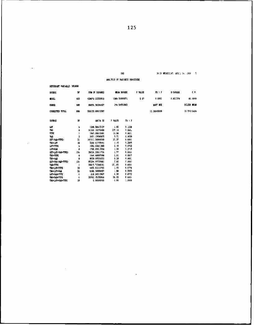
125

SLS 16:3! 4!ES'lY. AIU:L iw .9eo

ISLYSIS OF VIIACE PROCEDURE

DEPENDENT VIIIARLE: 011.181

SOURCE OF SUN OF SQUARES EA SQUARE F VALUE P ) F R-SOUARE C.V.

ODEL 403 439070.22330910 1009.52600871 6.07 0.0001 0.831379 80.0640

ENRON 4" 89054.58284487 179.54552993 ROOT ME D5 0 El l

COIECTED TOTM 890 528133.80615307 13.30046006 16.570)b464

SOURCE OF 91OVA SS VALU PD H F

LOT 4 1306.58413127 1.82 0.1230TRO 4 01304.18270409 127.14 0.0001TYPE 1 1947.09912401 10.84 0.0011VAR 2 2051.15 9HB55 5.71 0.0035SET (TATTPE) 31 141211.50848509 25.37 0.0001T 5 LOT 16 3300.41720441 1.15 0.3065IOTITPE 4 1552.03821205 2.16 0.0723LOT'iA 0 Il7l.05683204 1.24 0.2715SETtLOTIVU ETTPI) 124 30328.33011734 1.77 0.0001TBO'TYPE 4 1444.48607090 2.01 0.0017TBO#VAI 8 0039.00529322 8.29 0.0001SE?#'BO(IYjkffTEl 124 85304.65735091 i.33 0.000iVAR,TTPE I 289!5.72348101 18.05 0.0001

TBOvLOTTPE 16 4459.02212702 1.55 0.0176TBOLO07'l7 32 6106.29060467 1.08 0.3553LOrtwileTYPE 4 216.24212007 0.30 0.8772?RO'VA'TT PE 4 20702.15150600 28.83 0.0001TBOvLOTtATTPE 1 0.00000000 0.00 ..0000

126

LILLY!!!0 OF 9h:INCE ?2:s:,UOE

OEPODENT TA2llE: PERM0

SOURCE OF slim80C? SQtAs:! EAS 202A. F 'A-: 70 F 70.

MDEL 403 424969.8090.476 ... 4C. 2 .70 1.0007 :o.0§@

___ _ 49f :9541. 090110 3.4 11^45e 8001 E IM0.,Ef

:01U17!.D TOTLL 899 444492.8600486 0.27704744

SOURCE OF OVA SS F ViL!! ?I F

LOT 4 234.71011152 1.49 0.204',.2O 4 122!0.0256238 7 3. C.U0o!

TYPE 1 12817.17504500 325.30 0.0001via 2 219300.40495487 27891 0.0001SEMT IT'PE) 31 158217.40130984 129-53 0.0001

TBOtLOT 16 841.88154835 !.34 C.1?05

LOTv?!? 4 226.871?5761 1-44 0.2197

LOVU 8 589.60354735 1.87 0.0525SEtLOTfVii'TTPE) 124 8082.04662551 1.85 0.0001TBO#?TPE 4 32.9A368533 0.21 0.933378OYAS 8 3465.19045606 10.09 0.0001

SETBO(Vt?,'lY £ 124 14380.82704713 2.94 0.00.1

A19,?YE 1 0.00000000 0.00 !.0000

70OLOTvTTPE 16 915.81329835 1.39 0.1410TBOoLOT#Tli 32 3083.52190212 2.45 0.0001LOT.-FiR?YPE 4 14.20!15316 0.9 0.9853

TBTA0'TTPE 4 2455.22493057 15.58 0.0001

TBO#l0.VA'?ToPE 18 0.00000000 0.00 1.0000

127

SAS If-3i NEfEES!'Ay A. &ML iiep

ANALYSIS OF VARIANCE PROCEDURE

?UKEY'S tCWDEWTIZED RANGE I1501 TEST FP.D UARABLE: C0S!lOSE- SN:S TEST CONTROLS THE MYE I EXPERINENTWISE ERRORI RATE.

Or5 GENERALLY URS A 01GER ME Ill ERROR RATE TRAN REM~

WALPA0.O5 DF-496 NSE*459.2g6CRITICAL VALUE Of !TCDEIZED RAIGE-3.872ENImlNN SIGIIF!CANS D!FFEMECE6.1851

FEANS WITH TEE SLUE LETTER ARE NOT SIOIFICALY D!FFRCN.

TUXEY GROUING WEAN 9 LO0T

A 110.333 180 5

8 45.125 100 1

C 29.302 380 3

C 27.052 180 2

C 23.415 180 4

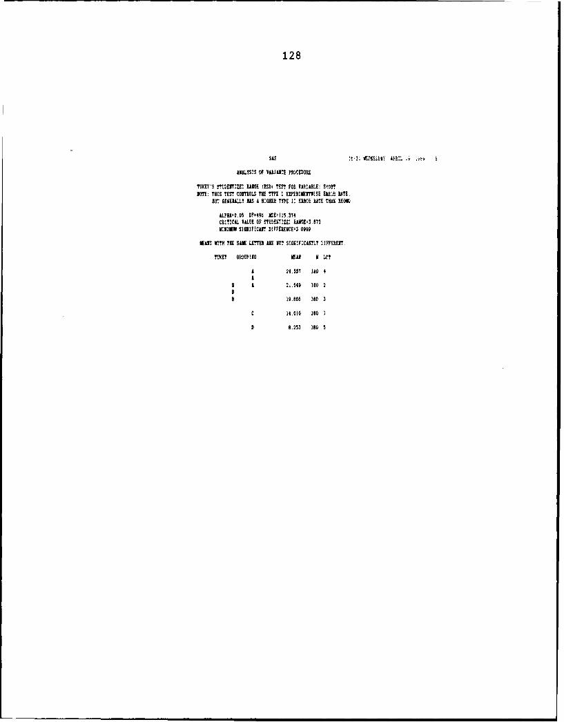
128

SS X f-2 ! iA -U IliAPIL r E

ANALYSIS OF VARIANCE POOCEDUXE

TOICEY'S MUNTZEDRAI~SEG EHSDI ?ES? FOR VAO.IAGLE: PSTNOTE: THIS TEST CONTROLS THE TI? ! 1 UEBIMENTWISE MR2 RATE.

BM' GENERALLY HAS A RIGMl ?! 1: ERR0R RATE THUO REMW

LLPBA:O.O5 DF-f9t IE:I!5.374CRITICAL VALUE OF STBOEI71- kUiO3.872MINI~M SIaJIFICAIT DIFFESENCE-3.OOAQ

NEL!!IS li1 SAME LM!! ARE NO! S!GEIFICLSLY '1FFERENT.

A 24.557 180 4

B A2~.4A 180 2

0 19.866 180 3

c 14.010 ISO I

D 8.253 ISO 5

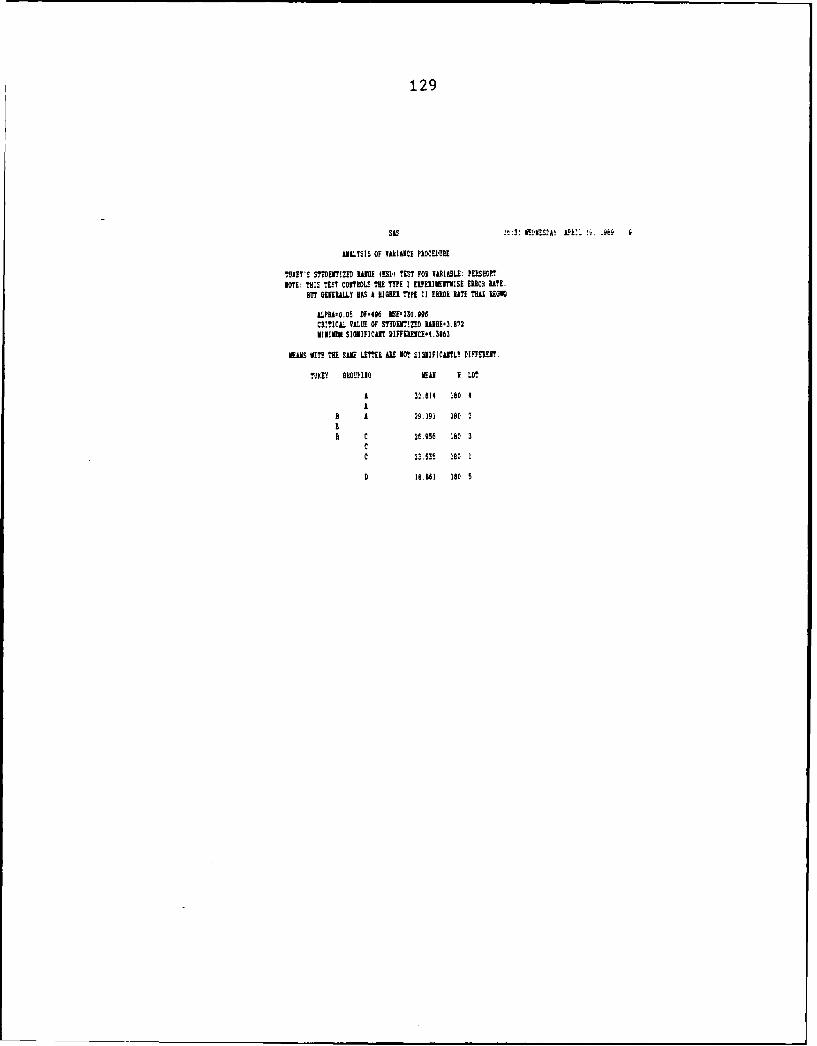
129

SAS !t:3! AVKfSlDV OR-

UILYSIS OF VAklAICI PROCEDUE

TOXET'S STUDEIZED lANA (HS11 'EST FOR VARIABLE: PUSHER?VOTE: THIS TEST CONTROLS TIE TYPE I ERIMEMTISE ERROR RATE.

BUT GENERALLY RAS A HIGHER TYPE 11 ERROR HATE TW EAR 0A

LPHI-O.04 RF-496 E-23O.996CRITICL VitAE OF SMT7ED AGE-.872M111EV SIGNIFICANT DIFFEWECE$4.3863

ELMS WITH THE SAVE LETTER ARE NOT SIGNIFIC11TLT DIFFERENT.

Tt'XEY G10OIIIIO VE~L I LOT

A 32.814 180 4A

a 2P.193 100 2

B c 2f.956 100 3CC 22.53, 1S0 I

D 18.861 180 5

130

UITIS OF VARIANCE PROCEDURE

TUXEY'S STUDETIME RANGE (RSO! TEST FOR VARIABLE! DLtERPIMT: THIS TES! CONTROLS THE TYPE I EXPERIMEMTISE EROR RATE

BUT GENERALY HAS A HIGME TYPE I! EROL RATE THUR REOWK

ALPRA'OOS5 RPF494 NSE-.S48Cl.TICAL VALUE OF SMUENTIZED RARE3.812hINlMN SIGN1IOANT DIFFERENCE:3. 8671

WAS V.TR THE SIR I.EOE ARE 10 SMAIFICLSTLY D:rFEORM.

TUffY WPM'J1 NEAR I LOT

A li..23 160 4

A 11.490 180 2AA 10.421 18O 1A

AH1.960 180 5

1 4.757 XS 3

131

SAS 16:3: EENEMAY LI:- !9. VS !I

AILYSIS OF VLIIAICE PROCEDlURE

?UICEY'S SUDEII ME10 IRSDI TEST FOR VIRI.!LE PElUUWEf: ThIS TEST COITROLS THE ?TT? : EIPEIIENTWISE EIROl. RATE.

BV! GiEEULLY UAS A Blom1 TYPE 11 ERROR WET THOR REGK

ALPh-O.OO l)P*IAO ME,31.4013CRITICAL VOLUE OF STUDENTIZED RM1E:3.872MNI MUJM SGIlFICANT DIFFEWECE.8NII

EONS WITH ME! SAE LETTER ALE 11O? SIOIIF:CLr.Y DSFFERT.

TORET ORTEPIMOG WEA N LOT

0 4f.2984 18V 2

A 05.9421 1A0 5

A 45.0113 IS0 1

A 44,003 1NC 3

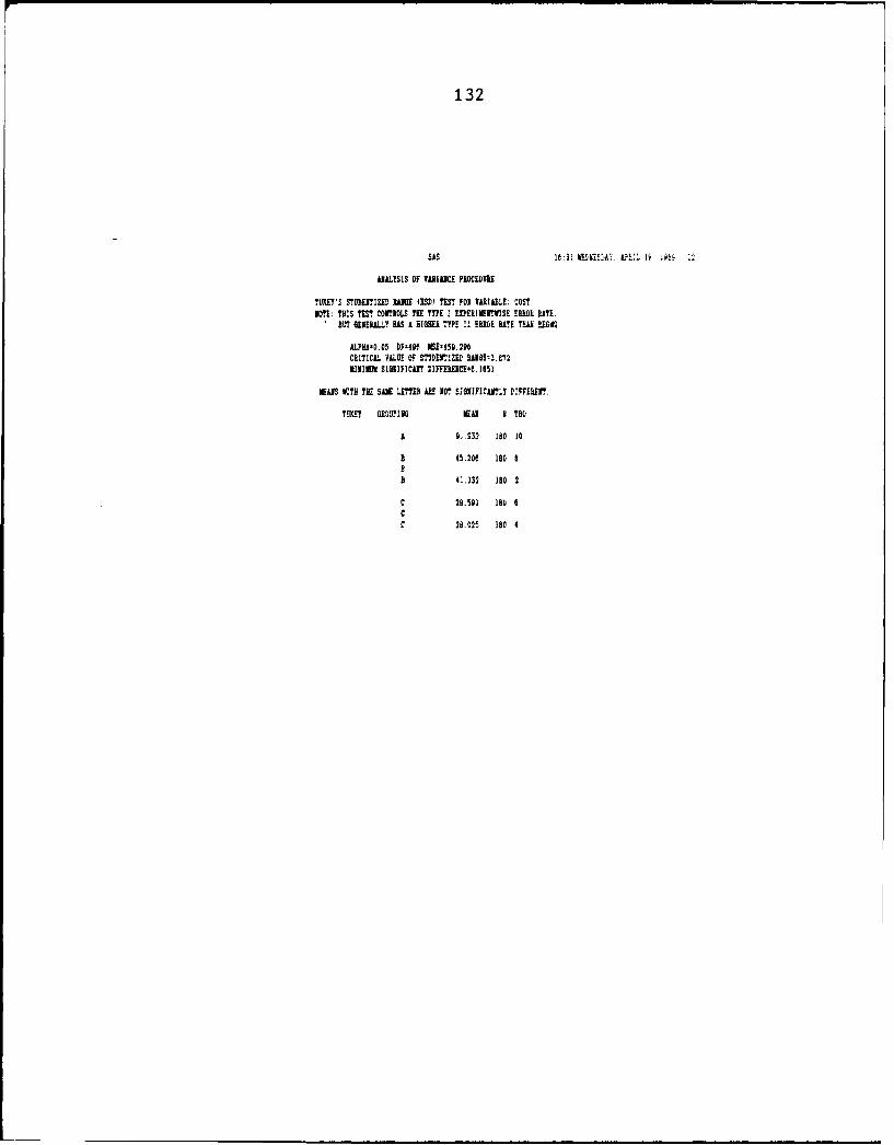
132

SM 1 : .Er.:AY. A2~. 1i :E :2

UALTSIS OF MAIICE POCEDURE

MTY'S rUIrIZ D NAI I USDI TEST FOR VARIULE: COSTiOTE: TH:S TST CONTROLS TPE 7W EERIlNWfSE ERROL RTE.

B' GEIERALLY US A I9l1 TYPE 1! ERO WTE TM 7G9

ALPU'O.05 DFY40 151'450.296CRITICA VALUE OF STUDEITIZED WUOE-3.?2

MINIMU SIOVIFICANT DIFFRE C :6.105I

EANS ME TIE SAE LE.TTER Aff 00 SO RIFICITY DIFFElEN.

TUXIEY G9R7ING EUA I 79O

A 91.932 180 10

B 45.206 160 8

B 41.132 180 2

C 29.591 160 6CC 28.025 180 4

133

ABAL.SIS OF VIRll!! PIOCEDUE

TEOTS STUDEKTEZED BABE lBSDi TES' FOE MAII: SBOiTNlDE THIS TEST CONTROL! T! MIE I EILBT S! MEDO E.

BE? GENERALLY MA A HIM~ TYPE 1 EM OE RATE THUR k!GV

ALPIkA:0.05 DF-40f 16E-115.374CRITICAI VALLUE OF STEDEITZED IAOE.3.0721MIM SIGEIFICAIT DIFFEE!CE'3.OVBE

EAMS r!HI TBE SHE LlEE AL NET SIIFICAILY DIFFERENI.

TUE'S 610UPIG NEU s Tat,

A 213.015 ISO 10

a 19.616 ISO a

0 10.822 1B0 4

C 10.312, 180 2

134

AILMS' OF VARAICE PIOCEE

TOVlET'S SUPEITIZED SINGE (HSF' TEST FOR VAOIAS3LE. PEOSROR?NOTE: THIS TEST COMTOLS TIE TYE 'EVEEIEMISE EROR RATE.

BaT GENERALLY WS A EIGGER MIE I! ERROR RWE THU AO

ALPI8A-0.05 RF-49f IE-23098CRITICAL VALUE OF STO2ErIZED RWOE:3.8'I2NIIMN SIIICIV? DIFFEWICE-4.3163

EAS VIPE THE SAE LETTER ARE 1OT SIABIFICANTLY DFFEMR.

TUXEY GRMWIB EAl I TO

A 30.0223 180 10

B A 27.601 ISO 4B

B25.440 100 2B* 24.211 180 6I

B24.082 180 S

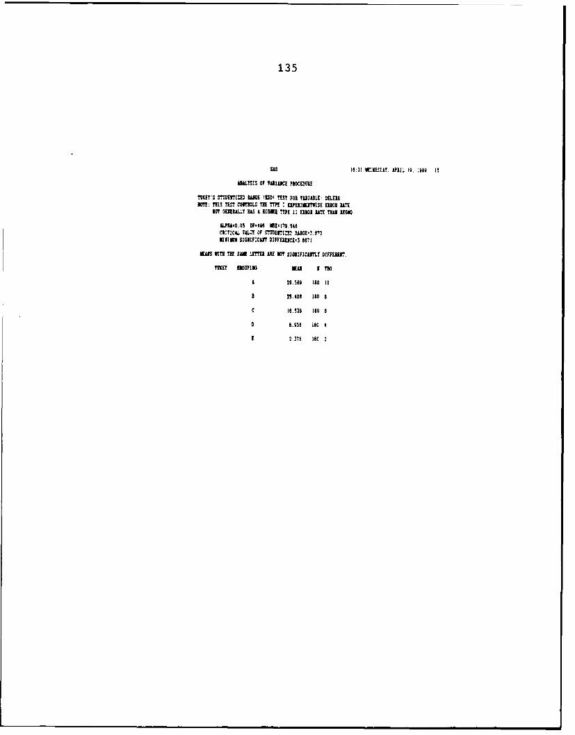
135

SAS !f3 L~ .ALPI'. 10. :J89 i

ALSIS OF VARIANCE ?IOCEDOU

ThOEY'S STUDEW!UZ LAUWE IISDW ?EST FOR OUIABLE' DEIIC?: THIS TEST CONTROLS THE TYPE I EIPEEIIEIISE EOROR WE.

BUT 3UEEALL.Y US A HIGHER TYPE li EROE LATE THUl EE9V

ALPIP-.O DF-494 *Esl70.549CEITICAL 7AL-41 OF SUENimE !al~.L'2miZUiE SIGEIFICAI EIPFEIUCE3.8571

MANS VOTI TEE SAII LFEER AM! N0? SIONIFICANTL DIFFERENT.

TEY EMUPING ll I 110

A29.599 110 10

25.408 180O

C 18.!38 LEO a

D 8.938 180 4

E 2.376 180 2

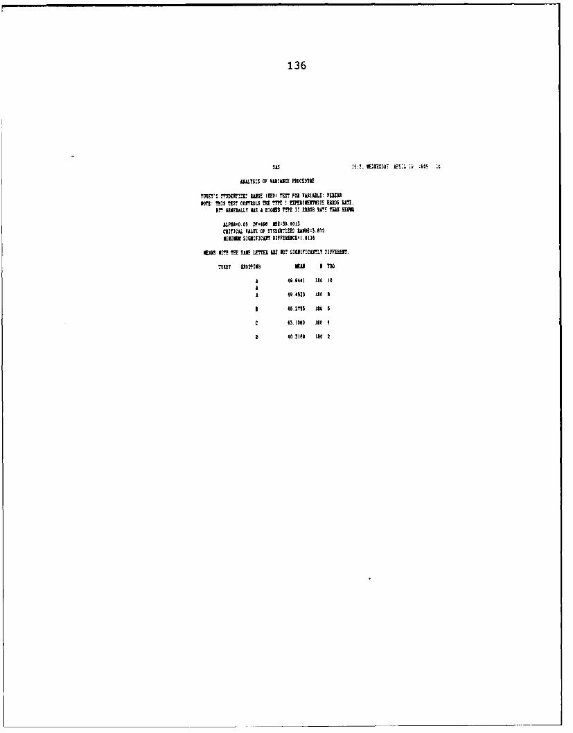
136

sis !6:3. .KMID--,AY PU.Z M !f

AILYSIS OF VAlIANCE PROCEDURE

TUKET'S CD nEI!ZE" IWANE (SI TEST FOR VARIALE: PIE'

IOT: THIS TEST CONTROLS THE TPt! I 1PERI IST ! EDROR RATE.Ilt? GENERALLY lAS A EIGR TYPE I EDOR WATE THAN REM

AL-,O.05 DF-40 MEl39.4013CRITICAL VALUE OF STUEIR!D IZ lIGE-3.872IIMUN SIMIFICAlT DIFFERENCEI .8116

WARS VITH TE SAE LEM ME 10! SIGNIFICANTLY DIFFEIMT.

TYKES GROPINIG LEAN I 510

1 4.0441 180 10

A 49.4533 180 8

3 46.2755 180 6

C 43.1000 180 4

D 40.3160 140 2

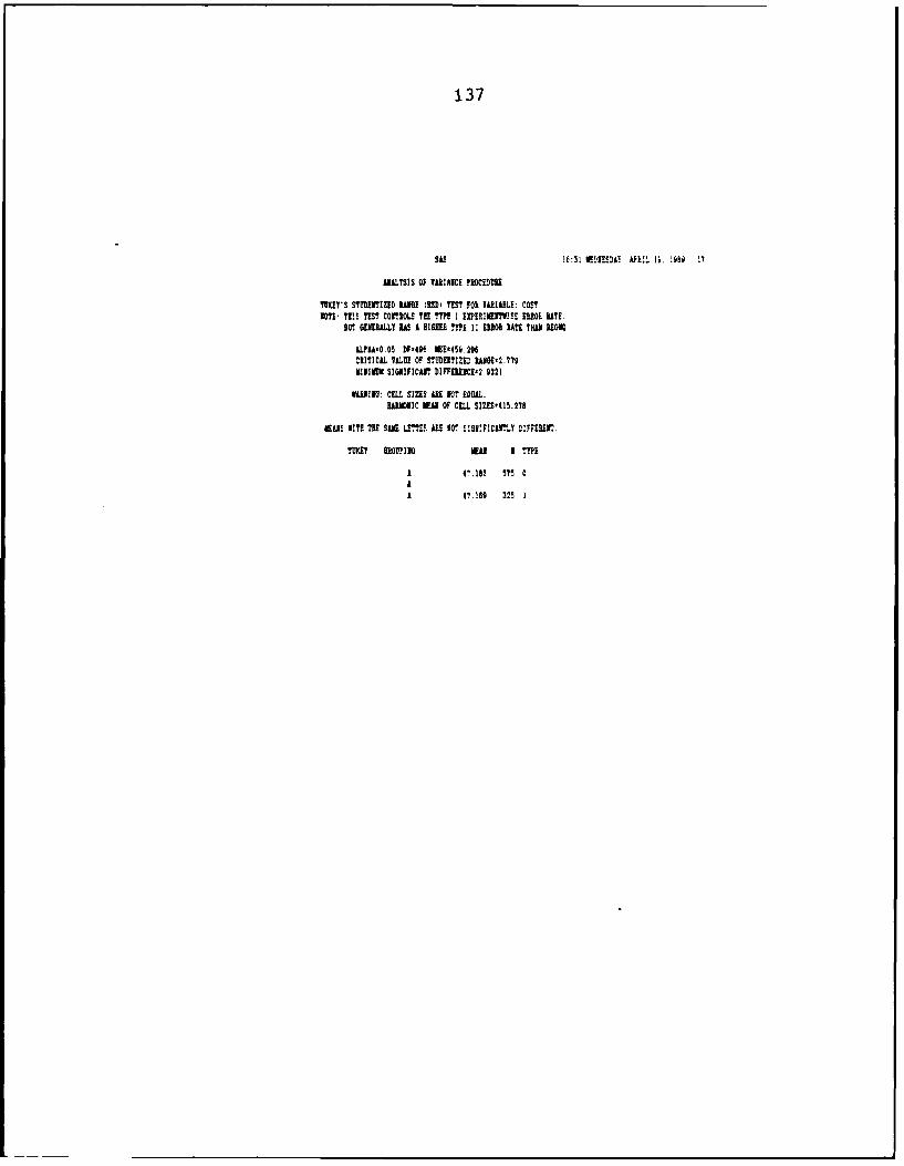
137

OhS e!:3! WA!SDo oA:. 1;. MOh

ANALYSIS OF VARIACE PROCOIE)O

YUKEY'S SITEENTIZCE E lDi TEST FOR VARIABLE: COSTNOTE- THIS' TEST CONTROLS TEE T"A I EIPEDIEIMSE MEOO RATE.

BOT SERALY HAS A AlOHA TYPE I! MELO RATE THUREO

ALPAA-O.OS DF'40f E-45i.29CRITICAL VALUE OF STUDEATIZED IANOC2.7791111113M SIGNIFICANT DIFDME-.2221

1101110: CELL SIZES ARE M0' EODAL.HAIDNIC MEAN Of CELL SIZES-415.27A

11LN VITA TAE SAhE LTE LEE MO? S!01:FICANLT DIFFE119r.

TOUT GLOATNNG LN I TYPE

A 4'.102 5TE 0AA 47.169 325 1

138

AIALYSIS Of WL600JCE PROCEDURE

",SY'S !!'30UlZ RAWO OSis fl!~ PO. IAK: SHOrtlOT! This nrS coBKoLs TmE ?TE i EDvierrf ma05 RATE.

DO* GEREIALLY MO A KNlELM III 015110 KAM !W~ IEOw

A~l?AOO.OS DP~lof ME115.374ClITICAL VALUE OF STUEI2D kRlGE2.779KINVUB SIAIIFICir DIPVKKUC 4046

WUNO- CMt S:ZES W 0! EQUAL,KAOV!C RU OP CELLI SI£1S-415.218

EIAKS VITO ME! SUE LEME5 ARE NOT SIO!FICAITl.Y DIPFE-im.

mEETy iOUflO 1EAN I TYPE

A 17.9250 575 0

A 17.1538 325 1

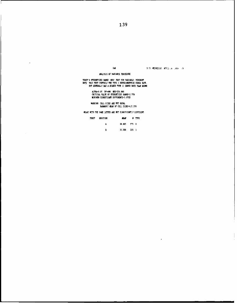
139

AALYSIS OF VARIANE PROCEDURE

TUXEY'S SgUDENTIZEf RANGE IRSDI TEST FOP VAIABLE PEUMOSATNOTE: TBIS TEST COrTL.0 TEE E I EI]ERINIr.SE ERROR RATE.

BUT? GENEALLY HAS A HIMHE TYPE I! ERMI RATE THAN REON

LPRAO.05 DF-496 iSEE230.996CRITICAL VALUE OF STOPR Y!ZED RMEIG:2.710MINIMJ SIGIlFICANT DIFFERECE-2.0723

VARYING: CELL SIS ARE NOT EOUL.HARMONIC NEAR OF CELL SIZES411.278

MEARS VITO THE SWN LXEE ARE No, SIGNIFICAN!ZO DIFFMO!N.

?TOO! OROrPING EU I TYPE

A 2e.495 S' o

8 2.336 325 I

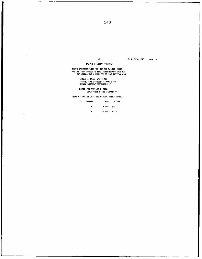
140

ANAL~YSIS OF TAIIC PROCEDORU

MEY'S ST'JDUIZED IME0 MDt TE FOR 1ASIALE DELEHlSOTE: TIF ETM COM~OLS TEE TTPE 1 EPERIETISE ERRI RAlTE

BCOIEhC4.Y RAS A LI TVPE 1! WOI RTE THU REM~

LPLPP0~,O5 ON*9 EI79.546CRITICaL VALl! OF STCOENIM! WIO27MININOM SIGNIPICAIT DIPPERENCE-3.827

WAlING- CELL SIZES LIE ICT EQUAL.AMV!C NEAU OF CELL SIZESW45.278

ERS IM.?! ESHE LETE ARC MC' SIONIF:lXYLY DIFFEUART.

MOE! GROLPIO NEUN K TYPE

I IR.5256 32t 1

B 15.4644 575 0

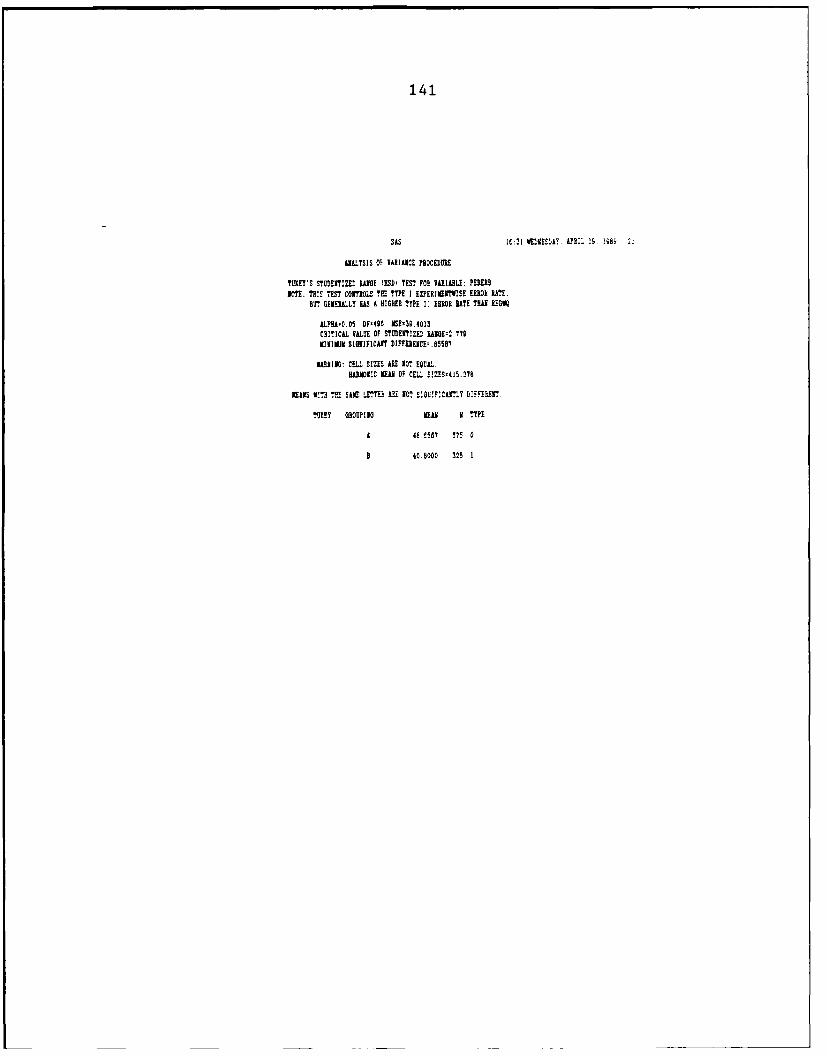
141

SAS lf:ll WE0!SD1!. APR!. 1 !8

LIALTSIS O1 VARIANCE PROCEDURE

? [TY'S STUDENTIMZ RANGE KSD) TEST FOP. VARILBLv: PERMB.

NOTE: T,£ TST CONTROLS TH! TYPE I EIrERINEYI S£ ERl I?!.BUT GENIRALLY US0 A HIGHER TYPE 1: ERROR RTE THAN 1 ,!W

AL?3AO.05 OF-496 IS39.4013CRIIC VALUE OF S0DEN3TIZE WLGE=2.,77MIIMUM SIG1NIFICANIT D)IFFE]LUICEz.8558"7

WARING: C..L SIZES ARE NO! E001.3AMO13I! NEAR Of CE.1 SIZES-411.276

NEWN V!?0 M0 SWM LETTER0 ARE 10! S031?I!ClTLT '!F?10!37

UK0 6ROUPING M v TYPE

A 48.!506 375 0

B 40.8000 325 1

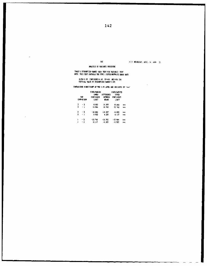
142

SAS :f:3. VEDWE!DLY. LE%:!i. m6s

ANALTSIS OF VAEI[AIE PROCEURE

IUKEY'S S.eDElT:ZEV RANGE IISDI TEST FOR VRIABLE: COSTVOTE: TilS TEST COTRIOLS ?I TYPE I EOPERIMEIRYSE EIROE RATE

ALPI-o.05 COrFID[fEMO.95 DF-496 ISE:45S.296CRITICAL VALUE Of STO 1 O1lZEI khiOE'3.325

COMPARISON SIGNIFICAIT T TI 0.05 LEVEL A11 INDICATED BY -,'

SIMULTNEOUS SIILTANEOUSLOWER DIFFEORCE llPPEk

YAP CONFIDENCE BETWIEE CONFI,ENECOMPARSON LIMIT REINS LIMIT

3 2 8.932 14.367 19.802 *,,3 1 13.664 18.702 22140 too

2 " 3 -19.802 -14.367 -6.932 oft2 I 0.553 4.335 8.117 '*t

I a -23.140 -16.702 -11.664 Its1 " 2 -8.117 -4.335 -0.553 .o

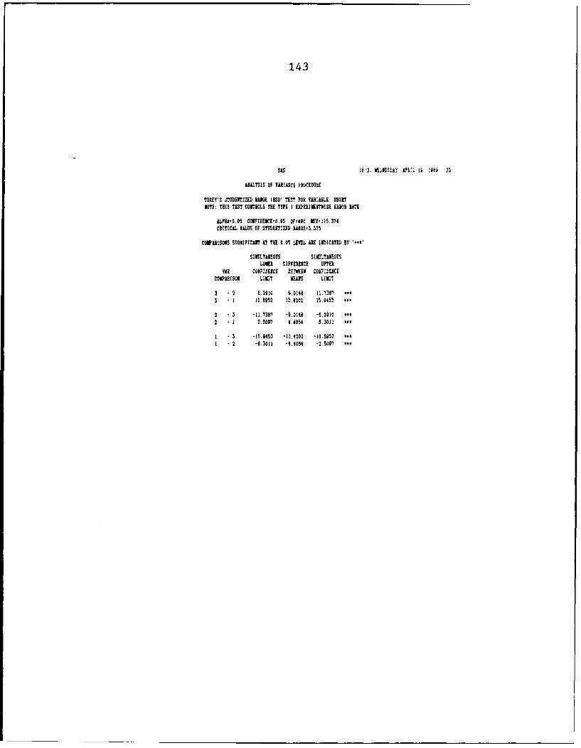
143

sis Ifl. EDJESth'Lv% n .1 h 0 25

ILYSIS OF VARIANCE PRCEDURE

?UXEY'S STUDUTN22 WOE IESDI TEST FORL VOJIAILE: SHORTNOTE: THIS TEST CONTRLOLS THE TYPE I ERSIEH ISE ERR0R RATE

£LPEA0O.05 COE?1LSCE-0.95 DF-49t lOE:1l5.374CIlITICAL VALVE OF SYUDiSIY1ZED kUOSEE3.325

COMPARIOS SIOIIFICAHY AT YE 0.05 LEVEL 111 INDICAYPIL BY '"W

SIMULTANEOUS S1MEY?1OUSLVID DIFFERENCE UPPERL

MA COYMEDSCE fETIhS!H COY:L!JCSCOMPAISOV 1.111? Ras LIMIT

3 -2 6.2910 0.0140 11.13873 1 100852 13.4202 15.9453 to-

2 -3 -11.1381 -9.0140 -0.2910 1'#2 1 2.5097 4.4054 5.3011 too

1 3 -15.0453 -13.4202 -10.8952 *..1 2 -6.3011 -4.4054 -'.500, lot

144

AUL!SIS Of IDUE PROCEDURE

TUKEYCS SMEEITIZED RANGE ICED) YES? FOR VIRIIULE: ?ERSHOIiOT: TEIS ToS cormNOs ME MTE I E!PE1IENTISE ERROR RATE

A.P9A:C.O! c3COINCE-0.9- DF-496 IE-210-096CRITICAL VALUE OF STUDENTIZED NIM,3.325

wei1SisM SIGIIFICAIT A? MI 0.05 LEVEL ARE EDICATED NT ..

SIMULTANEOUS SIIWJLTAIEOUSLOWER DIFFERESCE UPER

vAN CONFIUCCE ?ETWE CONFIDENCECuUFAAISOM LIMY NEWN LIMIT

3 -2 11.4351 15.2893 19.1434 .

3 1 19-9225 22.4954 26.0683 e

2 -3 -19.1434 -15.2893 -11.4351 fit

2 1 4.52138 1.2062 9.8885 ee

1 3 -26.0583 -22.404 -18.8225 e

1 2 -9.0885 -7.2062 -4.5238 e

145

SUS 16:31 WEIVSDAkY, A~kX: !96 25

ARLYSIS OF VARIANCE PROCEDURE

TMhET'S SMrNTIZED RANGI (ESR) TEST FOR VARIABLE, D1ENOTE: THIS ?EST CONTROLS THE TYPE I EXPEIIENF.SE ERROR RATE

ALPEFO.05 COIDU!E0..95 DF'49t ISE:179.546CRITICAL VALUE OF STUDEITIZED RUJGE-.325

COMPARISOIS SIGIIFICAIT AT TIE 0.05 LVEL AlE IDICATED BY "to'

SIMULTANEOUS SIlLTAlEOUSLOWER DIFFERENCE UPPER

VAR COFFEIECE 5ETMER COEFSEIVCECOMPARISON LIMIT EANS LIMIT

3 - 2 0.7936 4.1915 7.5805 .tt

3 - 1 1.2925 4.4424 7.5924 m--

2 - 3 -7.5895 -4.1015 -0.70362 - 1 -2.1140 0.2509 2.6157

- 3 -?.5924 -4.4424 -1.2025 t.4

1 - 2 -2.0157 -0.2500 2.1140

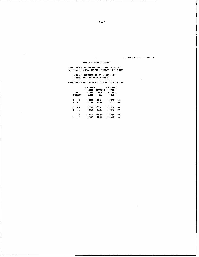
146

ANALYSIS OF VIRIAICE PROCEDUR

TUVEY'S SIVDENIZED lIIGE IHSD) 'ES? FOR TVILLE: ?ERlER

OM: ?I! TEST COITROLS ?BE TYPE I 1IFE11JME ISE D101 1?I

ALPIA-'O 05 COIFIDEICE=0.95 DF-49f MSE-30 4013

CRITICAL VALUE OF STUDENTIZED WO0E'3.325

COMPRISOIS SIJIFICAINT IT THE 0.05 LEVEL IE IEDICI IT BY '

SIMULTANEOUS SIMULIEOUSLaU DIFFE ICE UPPER

VAR CONFIDEICE BEWEEN COr:DENCECOARISOl LIMIT IJs LIMIT

3 - 2 32.3538 32.9155 35.5373 ot.3 I 45.1264 46.6020 46.07"7 .9t

2 - 3 -35.5373 -33.0455 -32.3538 t-,

2 - l 11.5487 !2.6565 1".7643 ,t9

1 - 3 -48.0777 -46.0020 -45.1264 ##'

1 - 2 -1,7643 -12.5 -1!.5487 of,

147

1LLYS!S OF V1Ill0E POOCEDOU

IS

TOO LO0 I COST SOT PE138OT D.01.009 PlOO

2 1 34 3i.351292 11.5868707 27.82'9877 3.1506861 40.1559350

2 2 36 45.068724 8.2236813 21.6130518 1.416322 4 0517132

2 3 36 41.6376K8 11.6952362 25.6601853 3 451604 40 6816922 4 38 3.587900 10.9064994 26.249059 1,30:!51 39.14C497,

2 5 36 41015926 8.1463710 24.0292803 ".4092040 40.35429t8

4 1 38 29.813956 12.7320075 22.12e'416 11.413005 47 IN1754 2 36 2;.16854 16.!790863 2e.,21069 c.n21727g 4. s87w444 3 38 15!,U9043 !6.3^74992 E14555 4t:.11,4 .w'7

4 4 36 23.110066 20.9125964 29.25:7025 10.2021562 4.385681

4 5 36 32.54886 14.3598951 24.8351298 6.4141020 4..084045

6 ! 36 36.870735 14.0820904 17.7349140 15 8985332 4! 5839146 2 38 23.!13733 22. 703861 2!.57VO76 1!.58'542! 4' 46.!-26 3 36 24.535388 1t.6623167 23.6!79099 15.4453788 4!.t573100

6 4 36 19.888236 26.!518947 31.3546905 20.9582918 47.87111896 5 36 43.268506 11.4764432 20.7745388 12.8003435 44.0034000

8 1 38 4.045366 10.22888! 18,2824! 2 32280 47.!7325088 2 36 22.264563 25.9883553 31.8475554 2k.1698494 50.2491919

8 3 38 27.93226 21.2523257 21.!721321 23.0071438 48.1391100

8 4 38 18 449472 29.8533942 31.7745990 25.7930292 4.86874588

8 5 38 111.21944! 5 7497322 !7.3A!3541 27.5418!58 5C.93, '50

10 1 36 74.74926 1.4 375 32 V3930 3.1110295 51 699)94?10 1. 35 1 .104"96 34.1782881 37.802202 21 09182 52.10972

10 3 36 27.032730 29.212882 31 6420208 23.4262M65 4!.80941!

10 4 36 1.26331 34.9206342 41.4!7874 32.7587800 5 1.153S19 5 36 323.516550 0.543915 7.5319683 30.6301549 5: 1

319711

LOT 1 "I I COST SHO8T PEOSIOIT DI0 m PRMT0

1 0 115 43.279024 14.8156566 25.5573803 15.2574145 48.52173371 1 65 48.390002 12.53821 18.9563308 18.4808570 40.62813982 0 115 28.078392 21.7194673 31.2755307 16.5895387 19.244903

2 1 65 26.898655 21.2478440 25.5021844 10.0830507 40.9976?6

3 0 115 29.588842 20.3116904 30.2502503 13.2843806 47.50090523 1 65 26.960157 18.0767320 21.1276352 17.3816838 40,.3240700

4 0 115 7.03509 23.J606455 34.1635841 15.683463 0.5910562

4 1 68 22.26879 25.7890233 30.4254802 22.6883172 42.1805868

5 0 115 110.902058 8.0220331 21,230DS819 16.4921929 49.3744530

5 1 65 109.327483 7.097877 14.6684231 15.0193806 30,88694423

LOT 1" I COS? S99T 0180T DE.0 0110

8 1 100 36.940171 10.4301340 16.2916460 15.5498420 31.2260771

1 2 55 48.878455 17.0631200 26.269?320 1.5844117 48.87914691 3 25 74 004228 21.5786230 46.4603644 11.3487409 80.3946828

2 1 100 25.01790 17.925678 24.3483272 15.9002832 35.4110560

2 2 95 26.914843 21.7005711 32.1724424 17.7196345 49.9M20858

2 3 25 36.431874 35.559174 42.0082980 23.3074812 83 76420363 1 800 28.524860 165054686 21.955850 148558359 35,9688523

3 2 35 28.353247 18.7504236 27,7688521 14.2001070 47.28476783 3 25 42928468 33.5604684 45.129;880 186.1877489 ?9.0936476

148

ItC :!; 12EIIAO 011. i0 196~ 2E

AiALYSIS OF ¥AIuCE PkOO]IC

W0 VU I COS? SHOI P5E§58O8 DEEU PER08

4 1 100 21.735546 21.1604820 28.5038136 18.085653 30.50132564 2 55 23.188191 26.2467084 32.7371 812 15.151776 47.847V020

4 3 25 30.634749 34.4257400 46.2216624 21.5156456 82.3623:72

5 1 100 lO 214585 6.1542214 12.8174229 14.1821!55 3!.20'9325

5 2 55 12.616491 9.3834071 2!.8074880 15.8886886 4'.60738.1

5 3 25 12! 786387 14.1624154 37.3524583 23.2351481 84.7042600

TA1 T11 I COS? SHUT PERSIOIT DLIU 0888E8

1 0 300 41.5524285 14.3540646 21.1855728 10.473310 34.3058300

1 1 200 45.8098269 14.5615458 20.5840810 23.9603071 37.10557732 0 !50 4.1299251 16.7934131 30.8011387 21.3729779 49,3230772 1 125 49.342676 21.3012687 25.1391303 9.6327150 4.7!110191

3 0 125 81.0571411 27.8572848 43.4403982 20.3180529 2,08186282

580 ME? I COST M8IT PERS900T DEL.01U 05151

2 0 115 42.3313970 10.8285809 289436864 2.79C122e 43.05!6950

2 1 85 20.075457 9.3973002 ig.2402997 1.651,1902 35 OWN194 0 1S 2e 7254624 16.6363644 29.4172402 8.3031069 45.8245444 1 55 2e.7850057 16.5966343 24.3870793 10.0599559 38.2877954

8 0 .15 22.2918941 19.8282751 25.1790293 15.327928 4.2387889

6 1 65 31.8891951 18.4552185 21.4344109 W85001083 41.03280918 0 115 44.1466057 19.6975162 27.0009387 23 582034 52 5085198

8 2 85 41.0814584 19 4720364 189184249 2e.639235 44.0470008

10 a 115 2 3954865 22.6387584 31.3358307 21.2618572 52,649987

10 1 05 81.1119594 23.8475737 27.6997830 33.7050021 45.1561785

590 v*i COST 3I0? PMIT FEL1 DELUI pti

2 1 100 41.33895 0.1807235 19.4527g5 1.5161418 31.130408

2 2 55 41705217 11.1145I88 25.8924474 2.3805842 42.1253775

2 3 25 39.045318 13.0694835 48.3873024 5.0648727 71.7832168

4 1 100 25 073 0 13.2371384 195481387 7.054689 33.1103388

4 2 55 27.766873 10.8395363 32.4104148 8.8527708 44.51247784 3 25 40.381828 23.0808814 48.082516 11.8522148 80.0087260

8 1 198 25.800817 23.6145105 18.0085042 16.3633748 35.82388386 2 S5 26.057500 10.5385731 25.3150704 12.4853855 4868945008 3 25 45.404832 36.55085 42.4863872 H.1003810 #?.14H202

I 1 10 37. 8898 14.5315112 1.5539412 22.7981010 37.5645054

8 2 55 41.106055 21.7146215 25.9480882 26,8021221 52.2S906858 3 25 71.576185 35.3136490 36.04H60 32.5828885 00.1351032

10 2 10 86.402220 21.814011 27.1703481 30.7109257 30.1501400

10 2 55 91.715678 22.0048053 31.011451 32.0681708 54.4848346

20 3 25 113.300865 31.271287 301250830 10.2885970 80 8524560

149

ANALYSIS OF VARIANCE PROCEDURE

510 LOT MI? I COST 5808? PE85808? D11.18 810100

2 1 0 23 41.371847 11.5583140 31.739!588 3.5408620 43.54797832 1 1 13 33.007506 11.6400322 20.3488423 2.4501285 35.81616622 2 0 23 43.744716 9.4854454 25.0289427 2.5149529 43.0366!782 2 1 13 47.411202 5.9805602 15.5695525 -0.3405582 34 7702852 3 0 23 43.755682 12.4505065 29.5076300 4.2145021 42.5141W6

2 3 1 13 37.872790 14.3588473 M0. "85800 2.1020174 35.87035772 4 0 23 3P.524310 1..M2763 3. .'OSOE38 0.02994 4.,.O697342 4 1 13 39 700390 11.067e942 22. :36896 2.4445111 3t5.01C7692 5 0 23 42.350622 i.8342823 263787 .816 40865

2 1 13 It. W5311 7.9292972 19.2375048 1.5903031 3WO444674 1 0 23 30.031925 13.0880958 2! 8954937 9.7516046 46035M5

4 1 1 13 28.874418 1-.1004120 18-5875848 11.5917498 39.04307154 2 0 23 30.398780 11.6410880 31.7427596 9.6020431 46.9429:394 2 1 13 27.042955 14.9154911 22.8239738 8.4934700 37.611224M4 3 0 23 2C.257796 !7.240'765 M5.3208377 ?.3350228 4!.24133744 3 1 13 24.827475 20.4172008 27.4l45930 10.4260948 U0.2196024 4 0 23 24.279529 22080M61 27.6439374 6.8673622 4!l!1~94834 4 I 13 21 .041015 2!.0609856 3L.7423638 1".5639917 U8.18826004 5 0 23 32.664293 14.3192257 2e.4831127 5.9594618 44.78053514 5 1 12 3,.339166 !4,42000 21.3669000 7.2104655 37.3M3210 1 0 23 34.469844 1!.6W4107 20.0651703 14.1850022 40.16627306 1 1 13 41.118t016 W1926 13.576TW8 16.930005t 40.9!!73926 2 0 23 23.818962 22.9869191 24.0012409 19.1315090 51.e5221060 2 I 13 23.250635 22.1208815 30.2550462 14.W510,14 U 38777006 3 0 23 24.625088 10.4927530 28.352!514 13.905917e 4E.280406 3 1 13 24.376680 17.1930831 15.24!9442 10.1690405 40.9007460 4 0 23 20.361M1 2f.1991013 329073 !E.692648, 50.1156116 4 1 13 10.435853 21,068!754 31.2351278 24.966382 43.51034928 5 0 23 38.184163 12.7690915 22.8720964 11.0016469 47.533088365 3 1 83 52.263881 9.1884490 17.0434601 15.9828526 39.07395158 1 0 23 42.787957 154632644 21.1513441 18.1724037 49.4641078

a 1 1 13 51.808476 14.8888553 13.2077544 30.2347764 44.22788858 2 0 23 23.55068 24.29"700 34.8526101 24.7710207 32.6125083* 2 1 13 20.044284 2b09793536 25.8901403 34.1811610 46.06794006 3 a 23 28.140454 22.4"847 25.083465S 23.132923S 52.29728618 3 1 13 27.568591 29.1117215 14.0802 2.7146166 43.168336Pa 4 0 23 16.9118640 29.2236013 32.4408209 22.3030091 52.71580001 4 1 83 17.548620 30.8475431 30.5059012 31.9703498 44.62807928 5 0 23 107.285161 7.02504H 21.3704448 2931112 55 45330468 5 1 13 118.439321 3.4934104 10.1706343 24.0117191 42.945404616 1 0 23 87.733916 16.278290H 29.11156817 30.032498 54.98572688 1 1 82 87.140710 16.6813172 34.007282 29.180243 42.09578718 2 4 23 18.176691 34.1121943 40.0521393 26.8260807 52.020192288 2 1 83 161734202 34.1658331 33.2622005 34.2330777 46.728496280 2 8 23 25.M5230 2908"0513 32.011!009 11.8335566 40 :473!!210 2 1 83 30.357230 28 3020073 29.26436!7 33.3266547 44.504984610 4 8 23 11.193430 L2.1730128 45.8405912 2 .8210217 152.0042210 4 I 13 14.6!7015 W871021115 30 41108 4!.4950911 47 7!!!!"I!0 5 0 23 !32.51505 2 t655 6 602541 3?,W92504 5! 005278610 t 1 13 30! 109'1 2.276823 !.4040,054 2! 2927528 43,6:165!1

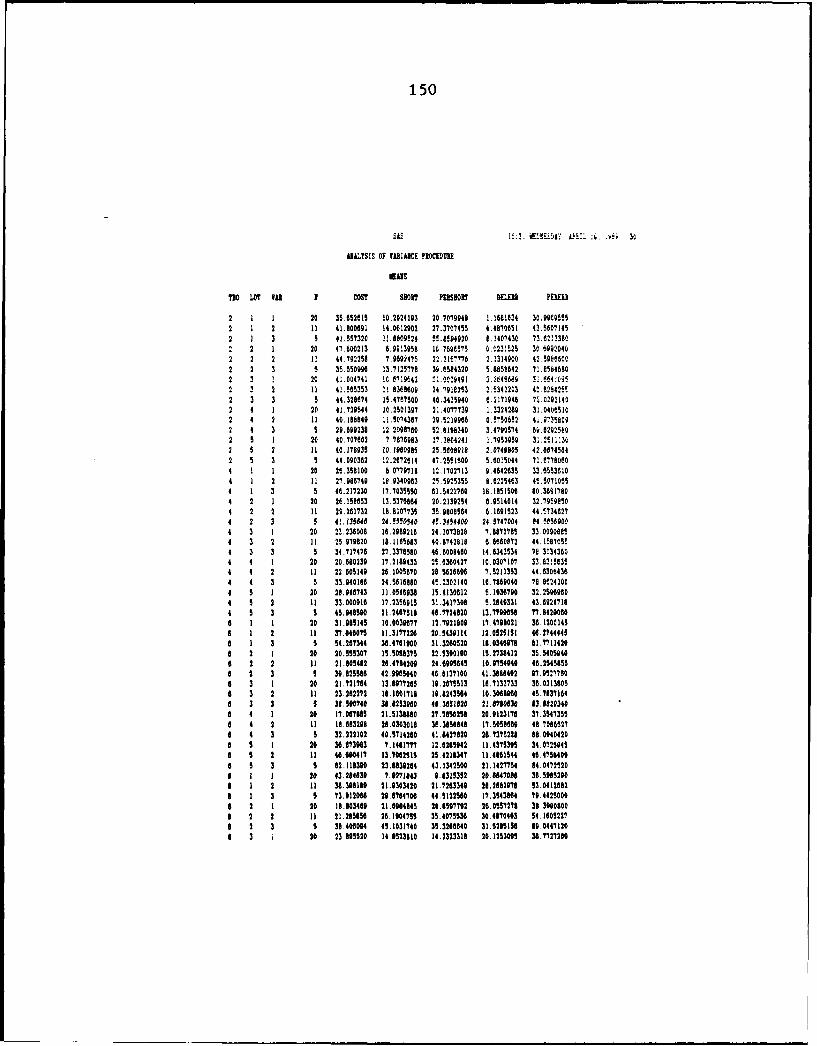
150

SE qi.£6z y ~: ~ 30

UI1.!SIS OF ¥ARIANCE PRODM

T0 LOT ViA I COST SBlOT PEUIBO? 9111 PErU

2 1 1 20 35.652115 10.2024103 20.7079948 1.1801634 30.9905552 1 2 11 41.8000691 14.0612902 27.3107455 4.4870651 42.5607145

2 1 3 5 41.557320 11.60924 !'.9594920 8.1407430 73.82123802 2 1 20 47.600213 .OM3958 16.769575 0.0231525 30.699020402 2 2 1! 44.702258 7.9692475 22.215"7 2.1314000 42.5960000

2 2 3 5 35.550905 13.7125,78 3.5584320 5.8858642 71.5646902 2 ! 20 41.004741 1C.6VI942 21.02491 :.264060 si.W5452 2 2 11 41.55353 i.83636860 24.7916253 2.5342203 42.82425!

2 3 3 5 44.328674 15.4787500 46.3405940 6.2171945 7..02921402 4 1 20 4.729544 10.2501397 2!.4077739 1.3324289 31.04055102 4 2 11 40.188849 11.5074367 29.5219968 0.!750852 41.973092 4 3 5 29.690238 12.2098760 52.8108340 3.4790574 60.6292590

2 5 1 20 40.707682 7.7876983 1.304241 1.7953950 3,.2!11:302 5 2 11 40.170935 10.1980905 25.5600918 2.0749805 42.80745842 5 3 5 44.090362 12.2872614 47.2551600 5.6015044 7517780604 1 1 20 2t.358100 b.0779718 12.1702713 9.46426835 33.6553610

4 1 2 11 27.986740 10.9340963 2.525355 8.6225463 4!.5071055

4 1 3 5 4e.217230 17.7035550 61.5422760 18.1851505 80.36017804 2 1 20 2E.1586853 13.5376884 20.2139254 6.9514014 32.79500504 2 2 11 29.261732 18.8107735 35.9808564 6.1691523 44. 346274 2 3 5 4.135646 24.550(540 4..3454400 24.5747004 04.505900

4 3 1 20 22.236008 16.2989216 24.3073828 7.8812785 33.009008854 3 2 11 25.979020 18.1185803 40.8742818 6.868072 44.1587055

4 3 3 5 34.717476 27.3378580 46.6008460 14.0343534 7e.30343604 4 1 20 20.880239 17.218933 25.880427 10.0307107 33.8136354 4 2 11 22.805149 26.1005670 28.5626606 7.5211353 44.6306436

4 4 3 5 33.940186 24.5615880 4!.2302140 18.7889040 76.8242004 5 2 20 20.O48703 11.0546938 15.4130812 5.1038790 32.25069804 5 2 11 33.000918 17.2358915 31.3417308 5.2849331 43.69247184 5 2 5 45.948590 21.2467518 46.7724820 13.70058 77.8420080

8 1 1 20 31.185145 10.003877 12.7921809 17.4790021 36.12001456 1 2 11 37.846075 11.317226 20.5430114 12.025151 46.2744445

a 1 3 5 54.267344 36.4761900 31.3280520 18.0348078 81.7711420

8 2 1 20 20.555307 15.5088375 22.5300100 15.2738412 35.5405940

8 2 2 11 21.105482 208.4784200 24.8995845 10.0754040 48.25458558 0 3 5 30.825588 42.99M5040 46.8137100 41.3880482 87.05:77608 3 1 20 21.7217164 13.8977285 19.2875513 16.7133733 36,03138058 3 2 D 23.202272 18.1801718 10.8243564 10.3068060 45.78371848 3 3 5 38.500740 3.8253080 49.381020 21.078030 13.1829340

S 42 17.07M 5 21.518880 27.1856258 20.8123176 37.35473554 2 1.83M8 28.0303018 3.3058848 17.5058880 48.7085627

8 4 3 5 32.222102 40.5714260 41.8427620 28.7375220 88.0404206 5 1 28 38.873943 1.14817'M 12.0285042 11.4375305 34.07259456 5 2 11 46.600417 13.700255 25.4216347 11.4011544 48.4758400

* 5 2 5 62.118300 23.8838264 43.134250 21.1427754 84.0472520

a I I 2 43.2"4638 7.9271 43 8.8315352 20.8847080 38.5902901 1 2 11 38.308118 21.0303420 21.7263340 28.2682078 S3.0412682

1 1 3 5 73.112046 28.06784706 44.5122500 17,2543864 70.44250008 2 I 20 18.103488 21.0984845 28.858792 28.057278 38.300800

* 2 2 11 21.28854 286.1804735 35.4075538 30.4870403 54.16052278 2 3 5 38.40004 45.1031740 35.3286640 31.521515% 89.04471208 3 i 29 23 885520 140523810 14.2323318 20.12%3M0 36.7727280

151

Sis 16:31 VEDCSDAY. 01%. 9. :Aeg 3!

ANITSIS OF VARIAMCE PROCEDUIR

EANS

1I0 10T Vo I COST SH01T PUSHOT D0.L1 P"FIR

8 3 2 11 27.546029 20.2922079 26.2001730 23.0844005 50.407764

a 3 3 5 44.935882 48.0363640 38.1188420 34.3645163 02.21718008 4 1 20 15.895039 24.2956340 32.8275536 24.5!20144 36.0240930

8 4 2 11 17.873941 34.6861464 27,1692995 2".1681112 50.33162366 4 3 5 29.933370 41.4523800 37.6944460 3e.8919077 96.2!97460

0 5 1 20 85.966324 4.4138723 12.2186053 22.6327448 32.02!54908 5 2 11 130425257 5.4130564 16.1371193 3 .4!2705 52.25,15188 5 3 5 170.69512 11.695564 33.8226220 4t.7141653 97.25!1379

10 1 1 20 47.420356 15.041287 5.562478 2b.9722724 31.759525510 1 2 11 86.360573 19,0721491 36.1151327 34.401344 56.0122018

10 1 3 5 154.067180 12.3559408 30.2117460 25.0287208 8f.7692560

10 2 1 20 16.191307 32.4935060 33.5404823 3!.2422929 3U.624921510 2 2 I! 17.429388 29.3939382 42.5174600 38.8349952 57.7231982

10 2 3 5 27.241050 51.4285720 42.8972440 12.8594764 75.299372010 3 ! 20 22.766305 26.7063497 31.0117101 25.28?3494 37.8059570

10 3 2 11 23.412759 30.3463191 27.0636235 28.8589308 53.245215510 3 3 5 52.069566 37.5259740 44.2174900 4.044C172 69.0354740

10 4 1 20 13.305022 32.5238095 39.8820718 38.6410049 42.255566010 4 2 11 1.5809749 30.9090900 42.0402555 28.0107093 52.5i37991

10 4 3 5 27.378848 53.3333300 53.5211560 19.6828350 79.0061200

10 5 1 20 333?.78110 0.366666 5.4464285 20.85!7086 40.4027100

10 5 2 11 312IS5927 0.3030303 7.5757573 30.1346145 52.6481700

10 5 3 5 306.077680 1.7142858 1!.7777774 34.8773286 93.1520580

LOT VAI TYPE I COST SHOR PERSHOB? D.L PEI,l

I 1 0 No 30.853670 11.5792636 16.272969 10.8061813 34.4807863

1 1 1 40 46.0M0823 8.7289396 16.3196196 22.60653331 36.3440132

1 2 0 30 42.525395 15.6052450 26.6819516 22.4171087 50.0428373

1 2 1 25 52.102128 18.7556000 25.775005 11.7851753 47.4827104

1 3 0 25 74.004228 21.9780230 46.490344 17.3487409 80.39468282 I 0 00 23.700616 17.5401594 25.2170700 0.0437386 34.0531748

2 1 1 40 29.103552 18.4957000 23.0394267 24.8576000 37.44983002 2 0 30 29.872711 18.5329932 34.4473138 24.2828534 51.0519603

2 2 1 25 23.365022 25.6512640 29.4425906 9.6437718 46.0742354

2 3 0 25 36.431874 35.5591764 42.0082980 23.3074612 63.7642036

3 1 0 00 23.206741 10.2201810 22.8273806 9.5955491 34.1374248

3 1 1 40 31.412037 16.9334001 20172818 22.2457601 36.43549353 2 0 30 31.116688 17.4540610 32.9608750 18.2425696 47.9005807

3 2 I 25 25.037110 22.5060631 21.8552247 0.5471515 46.5457924

3 3 0 25 42.028468 33.5604684 45.1291880 16.1877409 79.0930476

4 1 0 60 21.357070 19.1081216 28.5435471 11.6339871 34.7499730

4 1 1 40 22.303280 24.1040244 30.0442133 30.2632577 39.12835504 2 0 30 24.00355 24.3814473 35.3552429 18.9703152 48.1330550

4 2 1 25 22.2130 26.4850217 29.595072 10.5684124 417.06418044 3 0 25 30.634748 34.4257400 46,2210824 21.5156456 62.3t23172

5 I 0 00 108.584046 7.2205970 13. 02691 10.4572035 34.5580008

5 1 1 40 100.160343 4.545059 1149441535 10.7068785 36.17018505 2 8 30 103.13446 7.9459191 24.1243104 22.0430425 40.4906550

3 2 I 25 123.00480 11.1083938 18.0272545 7.4100040 45.78823805 3 0 25 125.786387 14.1824104 37.3524583 23.2351481 84.7942800

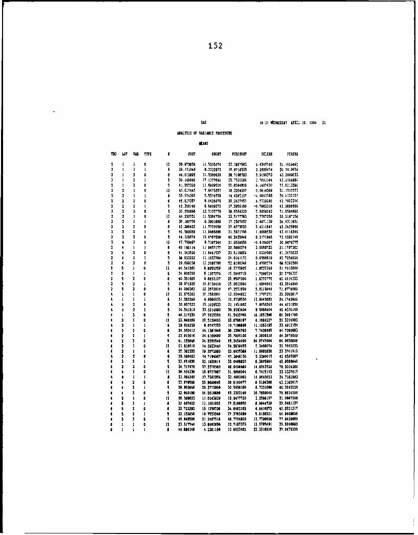
152

SAS 16:31 IEDSDAY. APRIL 19. 1989 32

AALYSIS OF VALACE PROCEDURE

TOO LOT ILI TYPE I COST SNORT IEOSROR? DELEH FEREAL

2 1 1 0 12 39.973659 11.5225074 21.1081563 0.4345740 31. 6640,2 1 1 1 8 29.171049 8.2222872 18.0718525 2.2605414 30.74100502 1 2 0 6 44.0!295 11.5200820 28.7196783 5.9104373 43-249033

2 1 2 1 5 39.146046 17.1107640 25.7520200 2.166.184 43.0,468602 1 3 0 5 41.557320 11.000524 55.8504920 6.1407430 73.62,33802 2 1 0 12 45.817445 7.9473557 18.3264207 0.0014309 31.!5065752 2 1 1 8 50.574355 5.5574559 14.434!127 -v.0042786 30.02202372 2 2 0 6 48.827357 0.0428478 26.2427457 4.5729246 42.7903300

2 2 2 1 5 42.350140 6.6609272 17.3856160 -017982316 42.36865602 2 3 0 5 35.55099 13.7125776 39.6584320 5.858642 71.85846602 3 1 0 12 44.220731 11.5264756 23.5177763 3.7767056 32.21872562 3 1 1 a 36.180756 9.390109 17.230702 2.407.213 30.03215'2 3 2 0 6 42.386423 11.7770050 27.457333 3.4211841 42.3425850

2 3 2 I 5 40.560008 11.9085880 21.5931796 1.450830 43.41143402 3 3 0 5 44.32674 15.4767500 46.3435940 8.2171946 72.0292140

2 4 1 0 12 42.758497 9.7197544 21.9538650 -0.4164007 30.94792752 4 1 1 8 40.186114 11.0457177 20.5886374 3.0556733 31.2707022 4 2 0 8 41.243530 11.8441537 33.811092 1.0320680 41.347033

2 4 2 1 5 38.923232 11.1033784 24.141172 0.026619 42.72540202 4 3 0 5 29.099230 12.2098700 52.896340 3.4790574 89.82925802 5 1 0 12 44.54165 6.8950250 l0.5775025 1.0525249 317013000

2 5 1 1 8 34.058358 8.1287070 11.58 715 1.7089!24 30.!75632!2 5 2 0 6 40.351685 t.8853127 25.0597200 2.8370775 42.08243332 5 2 1 5 30.071830 10.8134414 25.0022980 1.4004842 43.3604840

2 5 3 0 5 4.000302 12.2672614 47.2551600 5.015044 71.8770024 I 1 0 12 22.875302 10.1592841 13.0344822 7.1707271 33.30936174 1 1 1 8 31,582299 4.9580035 10.8739550 12.9045682 34.17436004 1 2 0 8 30.857532 15.1020532 21,451082 7.8856345 44.40218504 1 2 1 5 24.541810 23.5314680 30.0293404 9.5008404 46.8330100

4 1 3 0 5 40.217230 17.7035550 01.5422780 18.1851506 80.36917004 2 1 0 12 23.848260 10.5129403 23.8768167 4.1681227 32.33249834 2 1 8 8 29.824229 9.0747555 14.7190886 11.1263108 33.49121504 2 2 0 8 34.352412 14.1391841 34.1394783 7.742805 44.72609834 2 2 1 3 22.012916 24.4!0000 35.905100 4.2008310 44.3078004 2 3 0 5 41.135848 24.5550540 45.3454400 24.0747004 84.6508004 3 1 0 12 21.818510 14.2933440 24.5830455 !.3486074 32.768523

4 3 1 8 8 25.2025 10.3072880 23882338 11.6082850 33.37010124 3 2 0 0 28.086482 14.7194007 41.3946150 5.22001 42.65855674 3 2 1 5 23.481826 22.1930814 33.0408820 8.3905000 45.95888404 3 3 0 5 24.711478 21.3378580 48.8006460 14.8343534 ?8.30343604 4 1 0 12 20.404230 1.8727087 21.0666004 6.7415143 33.23376174 4 1 8 8 21.094245 17.7382954 32.4902002 14. 045053 34.7282862

4 4 2 0 0 23070588 25.8690045 26.0100477 8.5194396 43.21026174 4 2 1 5 20.955848 28.3772900 30.5458150 8.72318" 46.3243020

4 4 3 0 5 33.04016 24.5810080 45.2302140 16.7889040 ?8.8624200

4 5 1 0 12 26.598823 11.0243829 13.0477720 3.2598157 32.06875084 5 1 1 1 32.487422 l1.1001002 I.28OlO98 0.0044739 32.54811374 s 2 0 8 33.123303 15.1359728 34.8482185 4.8416073 42.6521317

4 5 2 8 5 32.133056 10.753540 27.3703480 5.8188521 44,0400004 5 3 0 5 45.948590 21.240758 48.724820 13.790058 7.0429000

8 1 1 0 I2 23.51"44 13.0492056 12.7187373 13.785401 35.5016602

6 1 1 1 8 44.66240 4.2301100 12.0023482 23.3316881 37.0475325

153

SU 15:1! EDIESDAY 00011 N. 10 32

OJILYSIS OF 90IIICE PROCEDUI

NEUS

?90 LOT VAR TYPE I COST SHORT P.ISO0? DEL1I PER01

6 1 2 0 6 30.875362 0.7222217 25.4506350 12.1901740 45.4914233

6 1 2 1 5 35.410932 13.2323238 14.655430 11.873244 47.2140700

6 1 3 0 5 54.267344 36.4761000 31.3260520 18.0346978 01.77114206 2 1 0 12 17.177751 14.600733 19.2804417 :0.504:260 34.430379.

6 2 1 1 6 25.821642 10.7234837 27.4268850 22.4202640 37.2059162

6 2 2 0 6 23.762530 22.6956233 16.7324483 17,.465332 46.30043676 2 2 1 5 19.457024 30.7777780 34.2601040 " 73C2490 43.718'040

6 2 3 0 5 30.8255806 42.0965040 46.8137100 4:1380492 97.9527760

6 3 1 0 12 17.917299 13.7037033 23.1301968 12.0929000 35.02757926 3 1 8 6 27.420461 14.1867612 13.4735031 23.6500832 37.5370825

6 3 2 0 6 26.402622 14.9603161 2.282183 11.07!1658 45.1811283

6 3 2 1 5 19.493852 21.9000980 16.07.3220 9.3849722 40.50082206 3 3 0 5 30.500740 30.8253960 49.3651620 21.6760630 83.88293406 4 1 0 12 16.128342 21.9675917 31.3279012 15.6526455 36.1603683

6 4 1 1 8 18.477109 20.8333325 22.4222126 28.8018259 39.13728626 4 2 0 6 18.944413 22.6851833 26.9272638 16.4019243 47.2098400

6 4 2 1 5 16.369960 34.4444440 45.3357900 18.83059080 50.5072500

6 4 3 0 5 32.222102 40.5714260 41.8427620 28.7375228 86.0404206 5 1 0 12 25.163864 0.9154082 17.1746405 f.3680503 33.184842

6 5 1 1 8 V .939162 2.9071970 5.8005247 10.04!1732 35.4041006 5 2 0 6 44.270573 0.09391517 17.3818603 11.1176997 45.8010267

a 5 2 1 5 49.503430 10.24:0546 35.06097800 : 0800600 4' 285!e0

6 5 3 0 5 62.110390 23,6839264 43.1342500 2:.142"54 84.04725206 1 1 0 12 32.805423 ?.0815424 10.12C7763 11.2t24813 34.61252338 1 1 1 8 50.003462 9.1866471 0.38k6736 34 7600495 39.2775375

0 1 2 0 6 36.016265 20.3703700 23.7330530 32 0739193 52.7852833

1 1 2 1 5 40.296498 23.8023084 19.3182732 22.0615400 52.14845008 1 3 0 5 73.012066 29.6764706 44.5122560 17.3543804 70.44250008 2 1 0 12 16.826624 18.6507033 30.9505042 15.6702480 35.6812433

a 2 1 1 8 21.7608736 24.7700212 21.2235567 41.6330475 42.4758350

0 2 2 0 6 24.819770 18.2539667 42.6449533 37.3413203 56.1148683S 2 2 1 5 17.285160 35.1142860 26.7226740 22.2619042 51.81530808 2 3 0 5 38.406094 45.J031740 35.326640 31.5205156 80.04471208 3 1 0 12 17.878703 14.6320307 14.571"13 14.1325960 35.4636900* 3 1 8 1 32.920745 15.4315475 13.7228875 29.1143784 30.73628008 3 2 0 6 34.667767 86.3690478 34410326 31.77391058 52.6970000

8 3 2 1 5 18.99944 25.0000000 10.545000 12.0569821 47.65M2808 3 3 0 5 44.935082 48.6363640 39.1108420 34.3845163 92.2171800* 4 8 0 12 14.974019 20.461100 28.9520525 11.5336307 34.0376275

0 4 1 1 S 17.275219 30.009200 38.6400052 43.979500 42.8037012S 4 2 0 6 17.700507 30.5079350 35.0403367 30.0118092 52.2186600

* 4 2 1 5 17.986062 32.5000000 17.7240548 12.7555656 48.0469400* 4 3 0 5 20.933370 41.4523600 37.8044460 38.8190" 06.2197460

8 5 1 8 12 76.323194 5.0603004 12.5063405 16,0564024 36.3837067

6 5 1 1 8 97.431020 2.0942301 11.7670050 32.4972576 40,49581258 5 2 0 6 112.404303 5.2588367 28.7448467 47.1343468 W6.7611183

8 5 2 1 5 152.052602 5.7321106 7.6078464 10.4348570 40.057920

8 5 3 0 5 170.6$6912 11.0998564 33.8226220 40.7741663 07.251376088 1 1 0 12 35.006220 15.2777763 22.2#62325 21.3845751 37.613428310 1 1 1 1 65.900560 17.0430492 31.4612700 40.0538185 40.47867210 8 2 0 6 61.064922 21.5476183 34.3611933 53,4163665 63.2863917

10 1 2 1 5 121.115354 16.1015860 30.2190600 11 7619535 47.2631740

154

SO&L:2 IEDIES080 A!0L 1 . :960 34

91LYSIS OF VLRIACE PROCEDURE

TBO LOT Mi TYPE I COST SMOT PERSHORT DELM Hi

10 1 3 0 5 154.067180 12.3550468 3.2117460 25.0287268 Bf.192560

10 2 1 0 12 5.032989 21.9206342 33.6542769 19.294555 36.6720956

10 2 1 1 8 M9.916 36.3528137 33.3922904 49.1537475 44.0541600

10 2 2 0 6 10.60148 28.333333 50.47t9433 53.9)00105 63.3:?063

10 2 2 1 5 14.822868 30.6666640 33.0540800 20.7440059 51.0:0554010 2 3 0 5 27.241050 51.4285720 42.6972440 12.8594764 ?5.29;3720

10 3 1 0 12 14.490465 2i."444450 20.3330208 12.60M57 3.~7

10 3 1 1 0 35.166067 2.3492059 15.0441440 44.2599700 41.%!'28?

10 3 2 0 6 24.040148 21.4444450 32.9368515 3.7135B13 5AMM71210 3 2 1 5 22.659892 31.4285680 20.0157500 1!.6333502 4.1961940

10 3 3 0 5 52.069566 37.5259740 44.207490 4.0446172 0.C25474

10 4 i 0 12 12.5i9354 2!.944450 39.4173164 24.6565457 3c.55(00

10 4 1 1 8 14.483524 40.6928562 40.5792050 59.6146937 41792695030 4 2 0 5 18.053757 25,0000000 52.2806700 40.93112448 56.747500

10 4 2 1 5 14.832940 37.099980 2P.7577500 12.5060667 47.696658010 4 3 0 5 2.378048 53.3333300 53.5211560 19.6e20360 79.005220010 5 1 0 12 368.291683 0,2777777 1.1250000 24.7492242 39.4581.25

10 5 1 1 8 282.00'750 0.5000000 i.92e6712 37.5054352 41.A29056 2

10 5 2 0 6 284,91433 0.1555555 13.6686893 4e.2842210 56.15tw6o

10 5 2 1 ! 346.232020 0.0030000 0.0000000 e.!550868 45.47416010 5 3 0 5 306.077680 1 '142858 15.777777# X4.77286 93.152C-50

APPENDIX E

ANOVA RESULTS -- GROUP II DATA

The following text provides the code used in the SAS

routine. Output consists of all subsequent pages.

DATA;INPUT SET TYPE VAR COFVAR TBO LOT COST SHORTPERSHORT DELERR PERERR BIAS;DROP TYPE VAR COFVAR BIAS;CARDS;

PROC ANOVA;CLASS SET TBO LOT;MODEL COST SHORT PERSHORT DELERR PERERR = LOT TBO

SET LOT*TBO LOT*SET TBO*SET;MEANS LOT / TUKEY E=LOT*SET;MEANS TBO / TUKEY E=TBO*SET;MEANS SET LOT*TBO LOT*SET TBO*SET / TUKEY;TEST H=LOT E=LOT*SET;TEST H=TBO E=TBO*SET;OUTPUT OUT=PLOTDATA P=YPRED R=YRESID;

PROC UNIVARIATE NORMAL PLOT;VAR YRESID;

PROC PLOT;PLOT YRESID*YPRED;PLOT YRESID*LOT;PLOT YRESID*TBO;

155

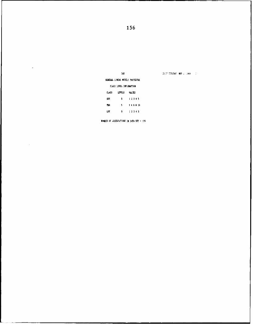
156

UIS 132 !DA! KAY.

GENERAL L.!!AiIDEL! PRCEUE

CLASSE LEVEL 11ECRNA?1AN

CLASS LEVELS VALUES

SIT 5 12 34 5

mAO 5 2 4 6810

LOT 5 12 34 5

DEE!E Of !SE6VAMONS IN DATA SE?: !25

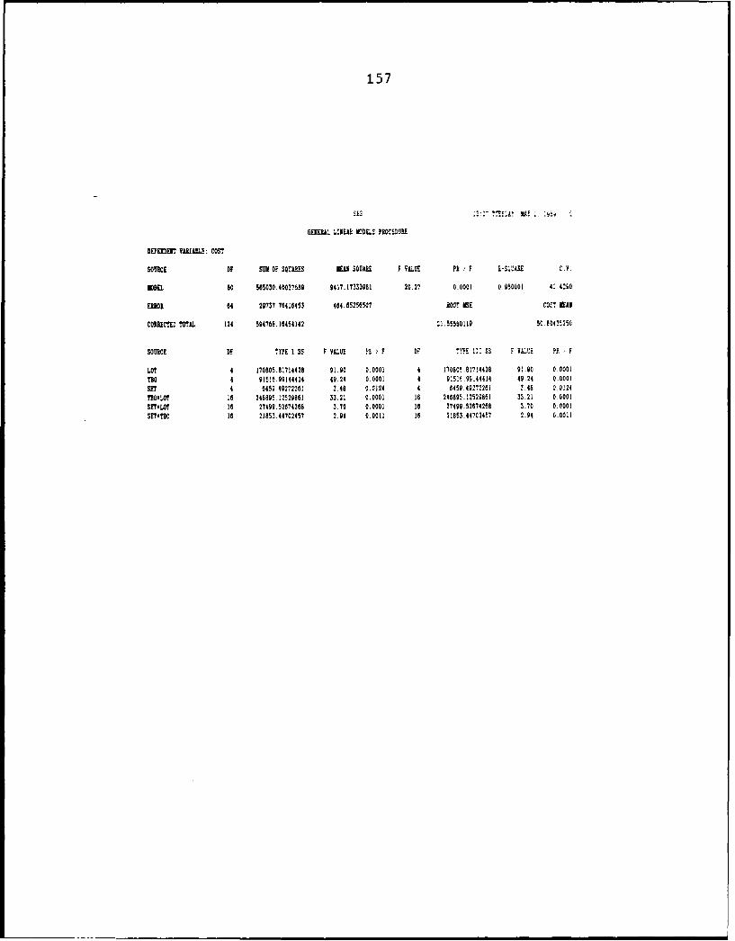
157

GEPM.A 'LI0Id ADELS PROCEDURI

DUESDEI? VARIJALE: COST

SOgmkC OF SOW OF SQUARES no SOULE F VALUE H F k-502Ik C.V.

*ODEL 0 585030.4003?5089 9417.17333961 20.27 0.0001 0.950001 41.4200

El]iO 64 29737.76416453 464.65256507 ROOT I E CO! MEAN

CODECTED TOTAL 124 594760.16454142 ..55010 50.804 R25,

soURCE OF CPE ISS fOE E )F OF 7YE1:Ss F VLUOS H PF

LO? 4 170805.81714428 91.90 0.0001 4 17080!,81714428 01.80 0.000i

TBO 4 9151!.99144414 49.24 0.0001 4 0.5!.9;44414 49.24 0.0001SET 4 0459.49272261 3.48 0,0124 4 6459.4922261 !.46 0.0124

TEOtOT 16 24689..2529861 33.21 0.0001 16 2406805.1252961 33.21 0.0001SET.LOT l6 27490.52674268 3.70 0.0001 1e 27499.52674268 3.70 0.0001

SEU*TRO le 21853.44702457 2.04 0.0011 16 21853.44702457 1.04 0.0011

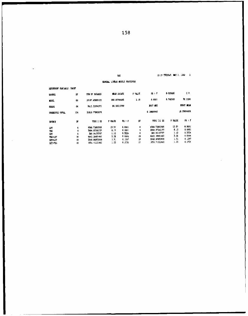
158

SAS 13:27 TUESDAY. MY 2. 389 3

SEXERAL LINEAR ADDELS PROCEDURE

DE IENT IARIABL: SNORT

SOURCE OF sum OF 59Q28R1 a" SQUARE F VALUE ?I ) F I-SQUARE C.V.

MODE 80 16197.45899103 259.95764985 3.19 0.0001 0.749508 50.2294

ERI 64 5413,32004373 64.58312588 ROOT ISE SHORT E"

CORRECTED TOTAL 124 21610.77903476 0.19%90849 16.35604909

SOU RE OF TYPE I SS F VALUE ) F OF TTPE III SS F VALUE P ) F

LOT 4 4589.73803595 13.57 0.0001 4 4589.73853595 13.57 0.0001

710 4 3084.87242157 9.12 0.0001 4 3084.87242157 9.12 0.0001

SET 4 380.04155767 1.12 0.3534 4 310.0415571 1.12 0.3534

"10QLOT Ie 4442.28461492 3.28 0.0004 16 4442.28461492 3,28 0.0004

SE7aLO l 2040.80953608 1.51 0.1247 18 2040.809536008 1,51 0.1247

sr#.BO IS 1659.7122.483 1.23 0.273t le le59.7:222463 1.23 0.27at

159

SAS 13:2T TUESDAY. 31' 2. 1989 4

GEREILL LINEAR 101W FROCOURE

DE1ENDET VARIABLE: POSB03?

SOIICE DF SUN OF SOUILUS MAN SQUARE F VALUE ?I P R I-SOUI.E C.V.

MDEL t0 36607.66270924 611. 6104665 2.30 0. 0006 0.603531 W9.3199

ERRO 64 16906.00641667 265.40700026 OOT IE FUSHOR EOAX

CORRECTED TOTAL 124 53673.74921591 16.21113513 27.46351051

SOURCE DF *YE ISS F VAL.UE I F D; ?T?." !::ss FOAZI F

LOT 4 4415.05882657 4.16 0.0047 4 44.5.85882667 4.16 0.0047

TBO 4 3417.40W5028 3.22 0.0100 4 3417.40857520 "..22 '..06u

SET 4 4Q55.qg267772 4.67 0.0023 4 45 .90 807772 4.6? 0.0023

TBOeLOT 16 4301.22395075 1.03 0.4340 16 439;.:22'0.5875 1.03 0.4349

SET#LOT 16 0201.27823573 2.10 0.0146 16 926..2 23573 2.18 0.0146

SETOTBO 1 10245.81032408 2.41 0.006? 1 10245.81032408 2.41 0.0067

160

SAS 13:27 TUESDAY. MAY 2. 1989 5

6EK.RAL LINEAR MODELS PROCEDR

DEPENDENT VARIABLE: DFIt

SOURCE OF SUN OF SQUARES MEA SQUARE F VALUE PR > F i-SQUARE C.V

MODEL 60 45730.57998833 762.17833314 3.04 0.0001 0.74013h 6>..7653

ERROR 64 10056.00094200 250.e7515534 lOOT USES DE:S Ea"

CORRECD TOTAL 124 61786.5893033 .5 83003897 25,43921/0

SOURCE OF tYE :SS F VII UDc F DY TYSi!:! ss F H.1 O F

LOT 4 1238.06104197 1.23 0.3055 4 1238.06I94197 1.23 0.3055

Ts0 4 17706.378375io 17.64 0.00N 4 .770 .of !'51 17..4 !.0004SET 4 12737.24578276 12.6 t.0001 4 1"737.245 276 1.69 D.00i

TbO#LOT 16 1345.14003183 0.34 0.911 16 !345.14003183 0.34 C.0991SETeLOT 1e 7350.04017087 1.83 0.0459 16 750.04017087 1.6 0.0459

S0vTBO 10 5353.71368571 1.33 0.2053 16 5353 71368571 -33 0.2053

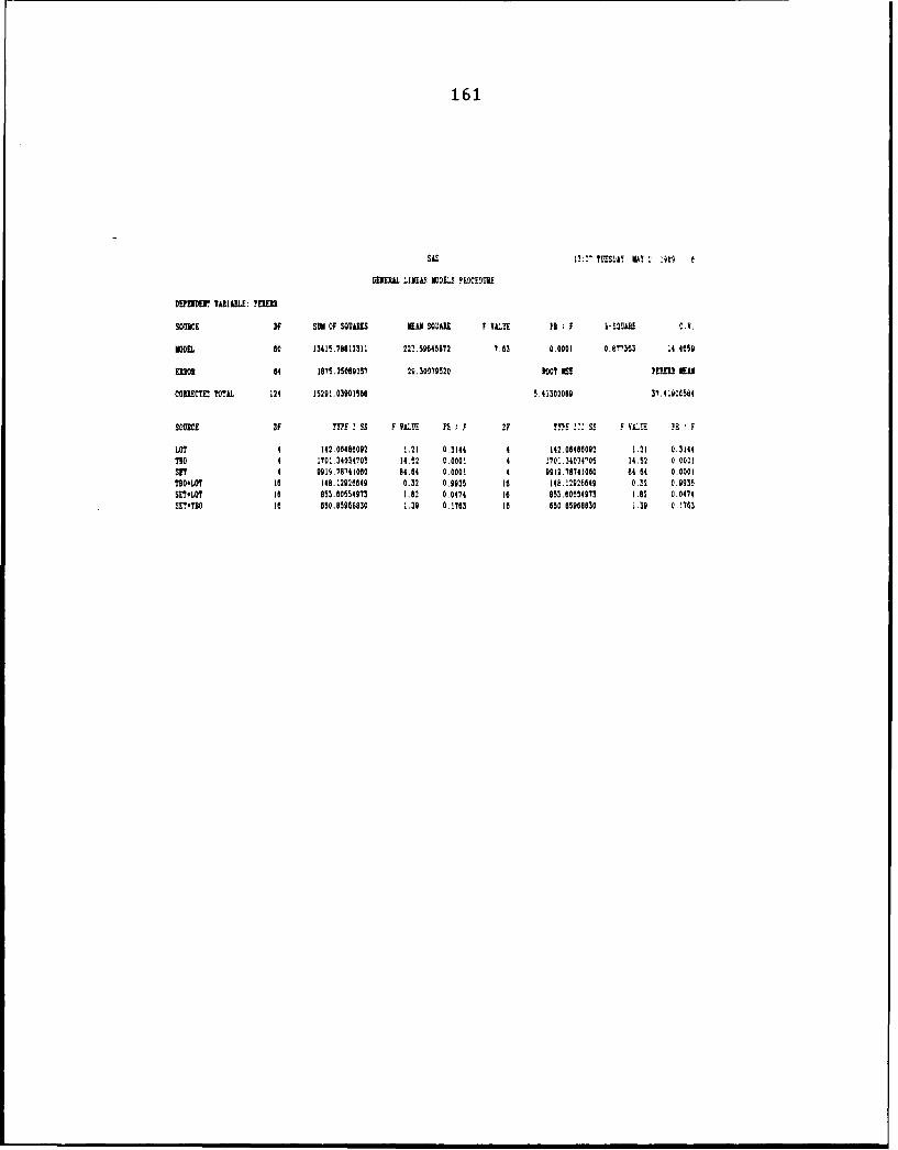
161

SS12: ?TES-1A. MAY ie9 f

GEJUMi .1JIAS wiEI ?ROCEDUU

DEEIII , VARIABLE PEIDI

SOOSIE DF SUN OF SQUAS lELi QUARE F VLUE ?I ) F i-l_10,R .V.

MODEL 60 13415.161112311 223.59046872 7.63 0.0001 o.e"363 14.4059

Wml 54 1875.25089257 21.30079520 w0? E PERM1 IIU

COIIDTC25 TOTAL 124 15291.03901586 5.41302069 37.41901584

SOMRCE DF ?YP . SS F YALUE I! ) F nF ?. ;:: SS F VL! FR F

LOT 4 142.06486092 1.21 0.3144 4 142.06480992 1.21 0.314420 4 1701.34034705 14.52 0.0001 4 170:.34034705 14.52 0.000!SET 4 910.76741000 84.54 0.0001 4 9919.7874100 84.64 0.0001T80O LOT 18 148.12926649 0.32 0.9935 10 148. !2926649 0.!2 0.9935SET-LOT 1 853.60554973 1.82 0.0474 15 853.0554973 1.82 0.0474SE*.TBO 10 650,85968830 1.39 0.!753 to 650.85908830 1.39 0.!763

162

SAS ',2 T'iDAY MAY

GENERAL LINEA MO E.S PROCEDUIR

THKEVS SYUENTIZED RAGE (!SDi IES? FOR VAiiAILE7 CO!!NOTE: THIS TEST CONTROLS TE TP ! EXPEIElVISE ERROR RATE.

BUT GENEALIY- HAS A HIGHER TYPEI I ERROR RATE lTIA REGN

LLPHA-0.0,5 DF-It 9117i1.72

CRITICIL VALUE OF SCE rIZ'Z, IGI 4.333I1l1N SIGNIFICIr DIFFERME-35. 924

VARS IETH THE SAME LTT' All NOT SIGNIFICANTLY DIFFERENT.

UKEY GRS? IINNEAR N LOT

A 121.43 25 5

3 54.29 25 1B

2f.92 2! 4

1 25.77 2! 3

1 25.62 215 2

163

SAS :t'Si: A Y '~

6115001 LISEM ES'ELS PROCEDURE

?UY'S sEEIZED RANGE l iSt" TEST FOR VARIABLE SHORTNOTE: T1I5 ?EST CONTROLS THE TYPE ! EPERIIEWSS EROR RATE.

? GENERALLY BAG A HIGHER TYPE 1: £.R0R RAE THAN 0W

CPAO.A5 DF-If I6E=127.551CRITICAL VALUE OF STUDErI2D UM11.

4.333

NIBINlM S!BB!FICNT IFF.REACEz91863

MEANS IT O THE SJiE L TTER Al NO? SIGNIFICANTLY t:-!nEl r?

A 22.137 252A1 21.270 25 3AA 19.551 25 4

N A .52 25 1

I f .300 25 5

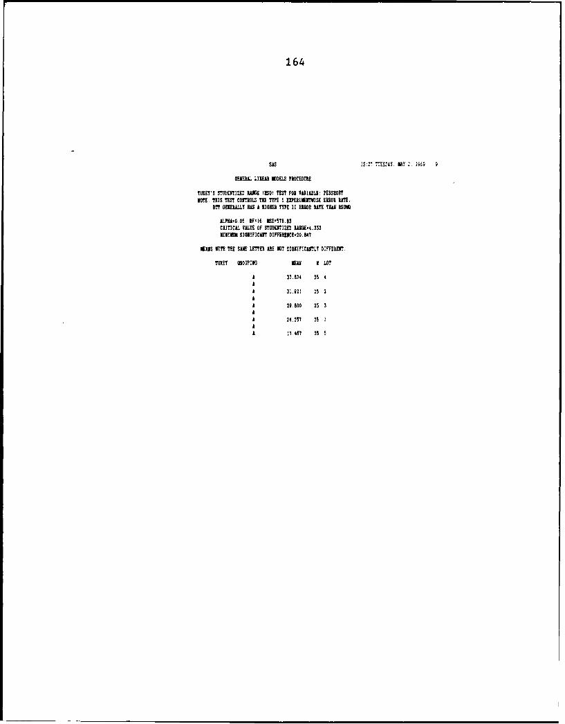
164

GEEA LINEM MODELS PROCEDOR

lUCEY'S SIUDEIIIZED RAGE IRSD TEE? FOR VARIABLE: PERMIOTNOTE: THIS TEST CONTROLS THE TTPE I EDERIEJTNISE ERROR RATE.

BUT GENEALLY UAS A HIGHER TYPE 11 ERROR RATE THAI BEOW

UAif0t.OS5I DF,6IE:SY.83CRITICAL VALUE OF STDEIIZED 1112-z4.333311131 SIC!? IlITl DIPIEOUCE-20.847

SNS WITH TEE SHE LETTER ARE VO? SIOlIICATLY DEFFEOEMt

TOUKT GBOUPIN NEAR I LOT

A 33.814 15 4

A 29.800 25 3

A 24.251 25 I

A !1.467 25 5

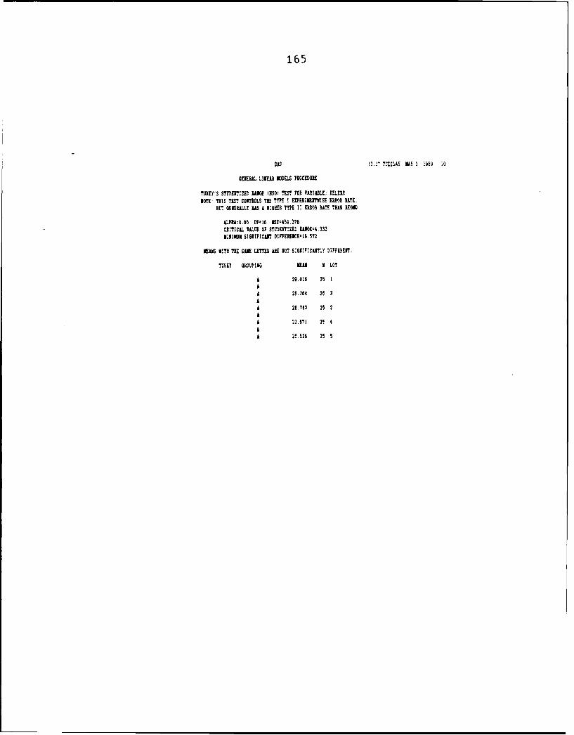
165

SAS !.2 ET A! MAY l ik i 0

GENERAL LINEAR MODELS PIOCEDURE

TIJEY'S STL.DErIZED RlGE RWD) ?EST FOR VARIULE: DMEL

NOTE: ?HIS TEST CONTROLS THE TYPE 1 EEIIErTWISE EROR RATE.BUT GENERALLY HAS A HIGER TYPE II ER OR ATE THA REM

AiPHAO.05 DF-I ME E459.378CRITICAL VALUE OF STUDE'IIM WUGE4.333MIIMUMI SIGNIFICANT DIFFEIICEIS572

EA S WITH TEE SAME LETTER ARE NOT SINIICAMT.Y DIFFERENT.

TMET! Gk0'YPIS MGEnl N LOT

A 29.016 25 1AA 21.264 2! 3AA 2f.742 25 2AA 23.871 2! 4AA 2C.526 2! 5

166

OhS 132, ?i.t.1. A Y :.: ; ;

GEIERAL LIUL! MODELS ? VEDDCE

?TK!Y'S SDENIZ RA NE I NO TEST FOR VA2iAEI: SM MNOTE: TE TEST CONTROLS TEE TYPE I EVEIIEITVISE ERR0 RATE.

BUT GENEIALLY US5 A RIMER TYPE !: ERROR RATE THU 0090

ALPEA:O.05 DFPI EI53.3504CIITICAL VALUE OF STURDEIZE W1GE-4.333INIMIUN SIGNIFICIANT DlIFU .ENCE.3202

NEOS KITE TE SAME LETTER E NO? SIG1IFICAIMLY IFFERE N.

TOKE! OROMPIO Ed I LOT

A 38.938 25 1AA 3E.16i 25 3AA 3.452 25 2

AA 34.474 25 4

A 36.044 25 5

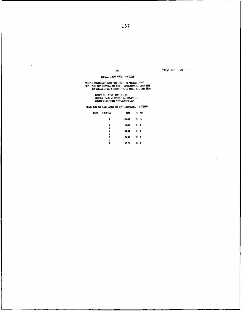
167

OS:SCta:o MAY 4

GENERAL LIVE EDELS PROCEDURE

?UIEF!S STUDENT2ZSI' HAND! IRSD) TEST FOBRIABLEk! COSTNOTE THIS TEST CONTROLS TTYP I EXPEDIENTI:SE ERROR RATE

tO GENERALLY HAS H OIlHER TYE I1 ERROR WAlE THi REOKj

ALPfO.05 OFi6 EE136584CRI!TICL VALUE OF TENTIZEL RAIOE,4.333313131 SIGI!FSCAI IFFEREICO:232.024

MANS ITH THE SME LETTER ARS HO? SIRHIF!AIrLT DIFFEREIT.

TUFT GROUPING MEAN N TO

a 101.15 25 10

B 52.24 258BI 38.10 25 2

3 32.88 25 HB6 27.70 25 4

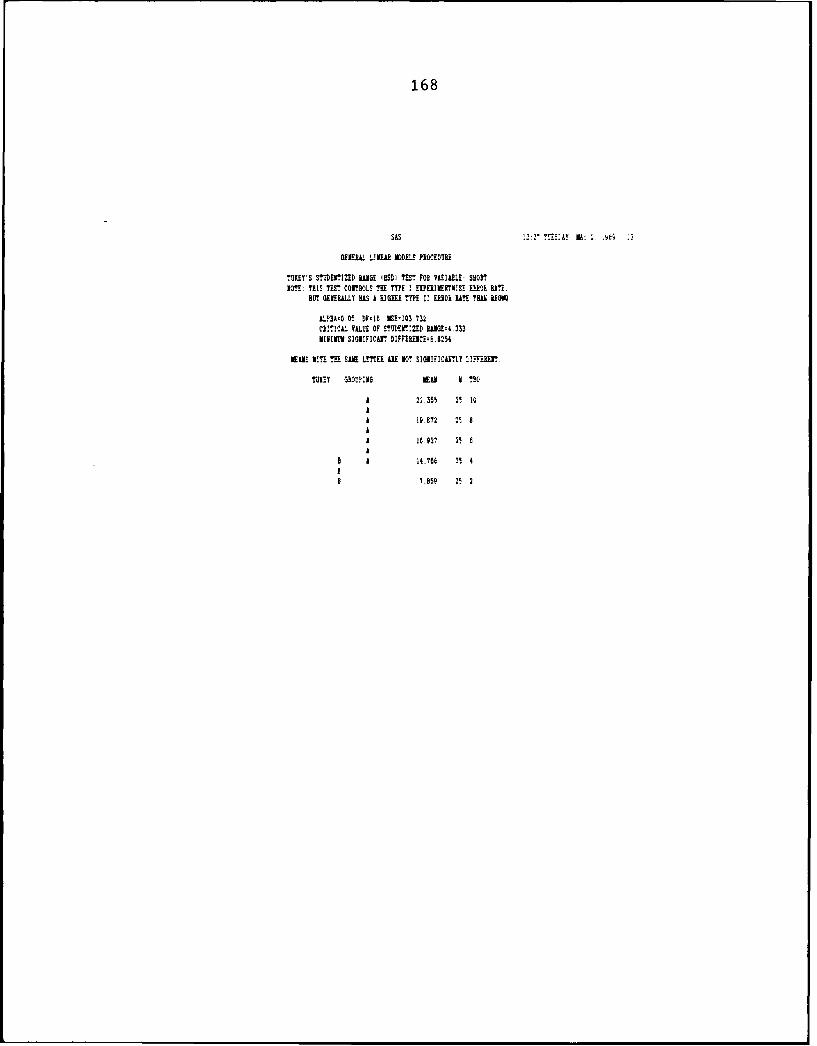
168

SAS 122,7!:SAY AMI,:E

GEMEOAL LIIEAI EDELS PROCEDDOR

TUEDYS STUDETIZEt WOGE IESDI TEST P0! VOEIABLE SHORTMYE: THIS TEST COMTOLS ?EF TTPE 1 EVERIEWISS EIROYD WE.

BUT GEEYPLLY HAS A BlOB! TYPE Il EROR RATE ?HM REMV

W100A~.05 DF-It MSE-103 732Ck!!ICLL VALUE OF !?TLEBT:ZED RNE-4 333KINI MUM SIGNBIUCAiT DIPPEBUCE-E8254

EWB MTE THE SAAB LETTER LIE KT SIOIPICOLMY '-IFPiREr

A24.355 2! 10

A19.872 1! A

a A 14.766 21 4BB 1-659 25 2

169

SAS 13:27 TUESDAY. MAY 2. 1089AQ i

GEVERA LIINO DELE PROCEDURE

TUErY'S STUDENTIZED RANGE lESD) TES' FOR VAIALE: PEuSEY!?NOTE! THIS TEST COE7IOLS THE TYPE I EVPENIMEETINSE ERROR RATE.

BUT GENERALLY UAS A HIGHEI TYPE 11 ERROR RATE TKREW0

ALRD-0.05 DF-16 NE440.363CRITICAL VALUE OF STUEWCTIZED WUGE"4.333MIIINUN SIGEIFICAIT DIFFERENCE"21.028

WEANS V YE TEE SAUE LETTER ill Or? SIGNIFICANTLY DIFFERENT.

TYKE! GRR'201E IcaN V TBO

A 35.AE1 25 10

A 30.453 25 A

A 26.205 25 6AA 23.877 25 2

A 20.921 2! 4

170

SAS 1:2,TMS0E'A MAY 2.9eg 1

GKERA2. 1.130*1 MODELS PROCEDURE

St'XE!'S SUDWIZED OAKS ! SDI TEST FOP VAiBUBLE: 001.130NOTE: THIS TEST CONTROLS THE TYPE I EVEEEEENTWISE 101Db WAE.

BrT GEEALLY HAS A HI00!! TYPE 11 E1100 BAnT! YO REGW2

A1.PHAA0.05 DF--1O NSF334-601CEITICA. ILU! OF! STYDEAY:ZEC, RAJOE-o .333MINIMUM SIGNIFICANT DIFTERIHCE:15.851

EANS WITH ?HE SAHE LETTER A&H 30! SIGHEFICAITLY DIFF!0!HT.

TOP:!! O0C!F1G MEAN K ?BA

A 36.478 2! 10

A 3'.083 25 A

B A 26.033 2! d

BB C 20 675 i4

C !150 25 2

171

SAS :2 .EEA MAY: ;-~

GEFERAZ- LINEAF MMCLS PROCEDURE

?UKETI S .TENI!EU RAIO! 'ESD! ?ES? FOP. VAPIAML PER'fNOTE M'!! TEST CONRpOL! MU MUE ! EVIEM E ERR,;ET.

fiU G!I!RALLY WE! I AGE !?E 1: MR WE TAN L!GK

iLPH=0.0 DF-If NF451 V?81CRT1CAI VALUE OF STUDEh'IZED AAGE-4.333M1N!KfM SIGVIF!:AII DIFFERICE-5.5266

NEII V!TH THE SAME LflT!E ALE NO! SIGNIFChITLY DIFFERENT,.

TSvflY 007F'ING la" N M

A 41 415 25 10

AA 31.25fr 2! fAA 1 M 949 2! 4

B A* i!94 2! 2

172

GKERA.L LI~L FriELE PEOCETYRE

floFEY'! STUDErIZED WOEG HOSD' TEST FOE V!AOS, COS!NOY!- THIS TEST CONTROLS THE TYPE !EIYERIWESE ERI-' RATE.

8T OEEALLO HAS A 0100!! TYPE TI ERHO RATE TAO RG

LPA:0.05 DP-84 EE-464 553CISYICAL UasU OFS sinr:ZE! LOGE:'970MIVINIM SIONFCNTAJ NPEEEJS~l-I7,J]4

EONS £559 THE SolE LTTER AE 10T SIO:FICAILT2* OEEU! T

YO1KE! ROMFIG 1EAN ET!

A R0. 1!7 2! 4AA 0950 2!

A 41.910 2! 2

A 42.E14 2

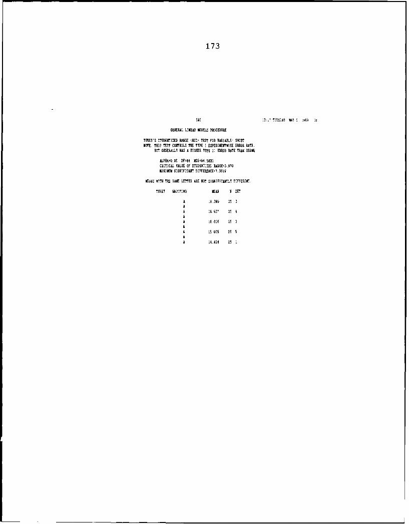
173

SAS B: 'S:R NY !~Q t

GENERAL LINEAR MODELS PROCEDRE

TUtER'S STERRIZED RANGE ESRi TEST FOR VRIIABLE- SHORTNOTE: TRIS TEE? CONTOLS THE TPE I EIPEOIMIRTISE ERROR RATE.

BUT~ GENERALLY UAS A HIGHER TYPE 11 ERROR RATE TRIO RROV2

AIPHA'O.05 RF'H4 MSE-z. 5031CRITICAL VALUE OF STUtINT:ZEL RANOE:3.O7OMIK!IM SIGiICLIT OIFFEENCE:Y.3O1A

NAWS rMYhTE SAME LEMTE AXE NOT SIGNIFICANTLY D:FFERLNT

TRAT GOO'JINO ESAR I E?

A .S209 25 3AA 160i2 21 4AA it.026 25 2AA 15 005 25 5AA 14-424 25 1

174

TV!!!! UD~W: E AN! H!! M7 FOE WAEL! EUKRT

Bt GU!RLZY WA A F:3EE: MPE !000 CEH -!A,3-

LpEAp'.!, !.F:64 EZ:!.0

i!AE0 7--? WAE Z!B- AL- 02£2'21Z

:ysr ~ r AS:?h EU

P A 0Th 2! 4

B A

B 20.69S 2! 3

B tRIt 25

175

SA-C 3:2' 7733.A' NA M 20

GIEEL ]INED MODELS PR03!DUR

?h4EY'S !!UDEIOZEE WGE IRS~t TEST FOR YAIABLE: DELERINOTE: THIS TEST COVThOLS THE TYPE I EUDERIHENTWE EOI: RATE.

EV! M!E UAL:Y HAS A HIGHER TYPE! : ER000 WEi THUA kEX

ILPHA-O.05 DF 64 MSE:250.875CH!TICAI. VALUE OF S3JDEV*.'ZlbL WOE-3.970MINION SIGHF!3Ckr DIFFERERl'15

EASS W:?E TO! SLE LETTO L AR NO! 510 OX'FOfTLY :IFrU..

TUflO 6ROUPING NEB SET

A36.23, 2! 4

3.A2.114 25 2

B 2!:555 25 5

c 6,662 25 3

176

OHS !3:. !M!OIY. MA

GENERAL LINEB MODELS PROCEDRE

TUREY'S STURDrIZED RAWG (13D) TEST FOR TU-iASILE PElRRNOTE: TH!S ?EST CONTHOLS MN TYPE I EXPEEIVENWSE ERMO WAE.

BUT GENEALLY NAS A HIGHER TYPE 11 ERROR RATE THUG REMV

WLHA-0.05 DF*64 IE-29.3008cRIIC~L VALUE OF METGEHIZED WGE'3.G70MININM SIGNIFTICANT DIFlEREHCE-4.2976

VAK VI!E THE SAE LETTER LRE 10? SIIU'F.CATLY DI'HTEOC?.

TUG!? GROUPING ME" N SET

A 521.711 25 2

8 39.114 25 4

B 36.155 25 5

C 29.8 25 1

C 21.502 25 3

177

13:21' M2EAV" MAY. !9 2'

U2VARIATE

VARIAiLEflY.SID

VDVWIS OUTXI(f DEF-41 EMENrS

| 125 SUk NS 125 10% 3a2 46.434 9%2 44.3288 LkWES? HIGHESTMLU 5.472E-13 30 8.0911-11 752 9% 8.4889 95% 25.2995 -45.9912 28.3848S02 D0 15.486! VARIANCE 231.821 50 E. 0.729911 982 1.8527 -4.9433 3.0022SKEWNESS -0.250 0881SIS 1.43372 252 01 -8.9072 18! -16.708 -43.9996 34.0422USS 29737.8 CSS 29737.8 01 KIN -45.8912 52 -29.1132 -30.847 38.3373ci 89999 S52 BEAM 1.38512 1% -45.978' -':.444 0~.424T: UA0 4.6737-13 P10B8T" I k1AiGE 92.4252S6 BANK 64.5 PIOB>*S" 0.8747 03-Ql 17.4514NM '. 8 125 MD! -45.9912D:8NORMAL 0.0755447 PRB)D 0.08

STEM LEAF 4BOLOT 8O81L PROliM PLOT48 6 8 47.5.4

3 8 1 83 14 22 89 22 0134 41 588878889 9 " *. *!011123444 90 55558687?77788899 17 .......0 111111222223344444 19 ......-0 43322222222,110 15 it*

-0 a99988877788885 18 ....-1 444433321100000 IS .

-1 77777886 8-2-2 7 1-3 10 1 ", '-3 0 ' I

-4 40 2 0-4 8 2 0 -47.54' 1

. . .. . . ...... ............- -- * - -- -.-..... ---........ -.-... ---... --.

ILTIPLT 71M.1.1 BY 10-01 -2 -1 0 *1 t2

178

SAS 2:2", ?:,AY dA! oM. :2

1.0" OF IU!b .!flUf L.EA.: A OBS. B 2 oe. ETC.

60

50

40

A

30 L

A

A

20 AS* AAA A A

* ~ AJJA

iLBDA

20L I* A0AO0A A

SA AAAUA AU ASWIABA I A

0 * AAUAAO* A EChO

0 A A A*I ECAIAB

BBI I AA D

-0 AAAAOOA AAIB AA

* A IA

-20

* A

-30 A

-40 * A

A A A

- -0

-00 -00 -40 -20 0 20 40 60 00 100 120 140 250 100 200 220 240 260 260 30K 320 340 380 380 400

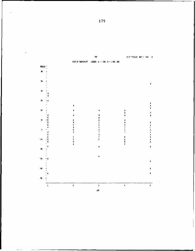
179

WAC 1!:2" ?tESDAY KA! l3e 24

PLOT OF YISSID'LO! LiE: A - 1 035 B 03. ETC.

TUSID-

80*

50*

40*

30 A-AA

30 'A

20 A A

AA20 1 A A

I CA1 B B A AB A

A AA

A AA

-30 13CC

1 A A

-20OT

180

PLOT OF YliS10'Th0O L!EED: A I OBS. B 2 OBS. ETC.

0

50 *

40 *

30 A

A A 5C A

10 B A'C C B

DB A

A A B D

0 A0 A B BAD FAA A

C B CB-10 *C C AC

*A A BA

AA

-30 A

2 4 a B 10

?DO

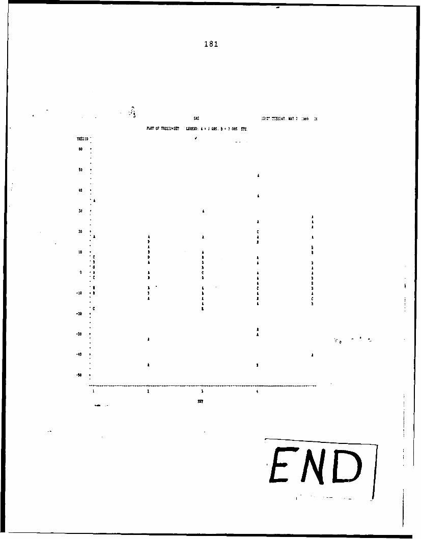
181

LOT OF Y,!! SE? LI A. I AB0 . I -2 ObS. -?C.

00

so

40

30 AA

A0 AA

20 1 Ca A AA

a bA

10 * a A

"aA A A

" - A AI -A A A

A B

A A I CA A Al

-20 *

-30

-40 * A

A I

-50

I 3 4

ENDI . . .